On the Strangeness S-wave Meson-Baryon Scattering
José A. Oller
Departamento de Física. Universidad de Murcia.#1#1#1email: oller@um.es
E-30071
Murcia. Spain.
Abstract
We consider meson-baryon interactions in S-wave with strangeness . This is a non-perturbative sector populated by plenty of resonances interacting in several two-body coupled channels. We study this sector combining a large set of experimental data. The recent experiments are remarkably accurate demanding a sound theoretical description to account for all the data. We employ unitary chiral perturbation theory up to and including to accomplish this aim. The spectroscopy of our solutions is studied within this approach, discussing the rise from the pole content of the two resonances and of the , , , and . We finally argue about our preferred solution.
1 Introduction
The study of strangeness meson-baryon dynamics comprising the plus coupled channels, has been renewed both from the theoretical and experimental sides. Experimentally, we have new exciting data like the increasing improvement in the precision of measurement of the line of kaonic hydrogen accomplished recently by DEAR [1], and its foreseen better determination, with an expected error of a few eV, by the DEAR/SIDDHARTA Collaboration [2]. This has established a challenge to theory so as to match such precision. In this line, ref.[3] provides an improvement over the traditional Deser formula for relating scattering at threshold with the spectroscopy of hadronic atoms [4]. This is achieved by including isospin breaking corrections to the Deser formula up to and including , the traditional Deser formula being in this counting, with the fine-structure constant and , the masses of the lightest quarks and . This is a first necessary step since the DEAR data have a precision of 20, of the same order as the corrections worked out in ref.[3]. In addition, one needs a good scattering amplitude to be implemented in this equation. The study of strangeness has a long history [5, 6, 7, 8, 9, 10, 11, 12] within K-matrix models, dispersion relations, meson-exchange models, quark models, cloudy bag-models or large QCD, just to quote a few. However, in more recent years it has received a lot of attention from the application of SU(3) baryon Chiral Perturbation Theory (CHPT) to this sector together with a unitarization procedure, see e.g., [13, 14, 15, 16, 17, 18, 19, 20, 21]. Recently, ref.[3] pointed out the possible inconsistency of the DEAR measurement on kaonic hydrogen and scattering, since the unitarized CHPT results, able to reproduce the scattering data, were not in agreement with DEAR. Later on, ref.[20] insisted on this fact based on its own fits, although they only included partially the CHPT amplitudes [22]. However, the situation changed from ref.[21] where it was shown that one can obtain fits in unitary CHPT (UCHPT), including full CHPT amplitudes, which are compatible both with DEAR and with scattering data. We extend in this work the analysis of ref.[21] by including additional experimental data, recently measured with remarkable precision by the Crystal-Ball Collaboration, for the reactions [23] and [24]. The importance of including the latter data in any analysis of interactions has been singled out in ref.[25]. The study of plus coupled channel interactions offers, from the theoretical point of view, a very challenging test ground for chiral effective field theories of QCD since one has there plenty of experimental data, Goldstone bosons dynamics and large and explicit SU(3) breaking. In addition, this sector shows a very rich spectroscopy with many I=0, 1 S-wave resonances that will be object as well of our study. Apart from that, these interactions are interrelated with many other interesting areas, as listed in ref.[21], e.g., possible kaon condensation in neutron-proton stars [26, 27, 28, 29], large yields of in heavy ions collisions [30, 31], kaonic atoms [32] or non-zero strangeness content of the proton [33, 34].
In section 2 we outline the theoretical formalism employed to calculate the strong S-wave amplitudes in coupled channels. In section 3 we review the data and fits delivered in ref.[21] and present an fit to the same data. In the next section we include further data and give new fits for the prior and new data. These fits are classified in two families, particularly based on the agreement or disagreement with respect to the DEAR measurement of kaonic hydrogen. In section 5 we discuss the pole content and its relation with observed resonances for the most representative fits. We end with some conclusions giving reasons to fix our preferred fit.
2 Formalism
CHPT is the effective field theory of strong interactions at low energies [35, 36, 37, 38, 39, 40, 41]. In refs.[42, 43] its extension to treat baryonic fields was pioneered. We concentrate here on processes including one baryon, both in the initial and final state, as well as in the intermediate ones. CHPT applied to this situation is usually called baryon CHPT. In the SU(2) sector it has proved very successful, see e.g. [37, 38, 39], and references therein. However, due to the relatively large mass of the strange quark, pure perturbative applications of SU(3) baryon CHPT suffer from converging problems. Notice that while in SU(2) one has as an expansion parameter, for SU(3) one also has , with , the masses of pions and kaons, respectively, being the latter much larger than the former. These facts make that cancellations of large contributions at second and third chiral order often happen with still sizable contributions, see, e.g., refs.[44, 45, 46]. Even more, for the case of S-wave I=0 scattering lengths, the CHPT prediction is a disaster [44]. This is due to the presence of the resonance below and close to the threshold. The situation changes once the chiral expansion is implemented with a resumation of unitarity bubbles [13], showing that chiral Lagrangians can be used in strangeness meson-baryon interactions reproducing this resonance. In ref.[17] the resummation of the right hand cut or unitarity cut (taking into account unitarity and analyticity) in the CHPT expansion was systematized to any two body process without spoiling the chiral counting and the CHPT series up to the considered order. This gives rise to the known Unitary CHPT or UCHPT. This work originated in turn from a series of previous works [14, 47, 48, 15, 16, 49], where similar techniques were already employed in meson-meson and meson-baryon production and interactions.
Meson-baryon interactions are described to lowest order in the CHPT expansion, i.e. at , by the chiral Lagrangian
| (2.1) | |||||
where stands for the octet baryon mass in the SU(3) chiral limit. The trace runs over flavor indices and the axial-vector couplings are constrained by . We use and extracted from hyperon decays [50]. Furthermore, , , with the pion decay constant in the SU(3) chiral limit, and the covariant derivative with . The flavor-matrices and collect the lightest octets of pseudo-scalar mesons and baryons , respectively:
| (2.5) | |||||
| (2.9) |
At next-to-leading order (NLO) in CHPT, i.e. , the meson-baryon interactions are described by the Lagrangian
| (2.10) | |||||
Here ellipses denote terms that do not produce new independent contributions to S-wave meson-baryon scattering at . In addition, , , is the diagonal quark mass matrix , and the quark condensate in the SU(3) chiral limit. The couplings present in eq.(2.10) are fitted to data, with the subscript referring both to , , as well as to 1, 2, 3 ,4. Nevertheless, in the fitting process we will impose three relations to be satisfied between the , hence decreasing to the same extent the number of free parameters.
From the Lagrangians of eqs.(2.1) and (2.10) we calculate the and meson-baryon amplitudes. The expressions in the canonical basis for the baryons#2#2#2The canonical basis is given by the fields , , such that , with the Gell-Mann matrices and the matrix given in eq.(2.9) are given in ref.[17]. The expressions are given in ref.[51]. The calculated chiral amplitudes are then projected in S-wave according to,
| (2.11) |
where is a generic meson-baryon scattering amplitude of channel into channel depending on , the total energy in the center of mass frame (CM), angles and the initial and final spin of the baryons, , with . The result of eq.(2.11) does not depend on the particular sign for .
We have ten meson-baryon coupled channels with strangeness (or zero hypercharge): , , , , , , , , and , in increasing threshold energy order. Each channel is labelled by its position (1 to 10) in the previous list. We denote the CHPT amplitudes at by and at by , with subscripts indicating the scattering process , so that the CHPT amplitude up to and including is given by . We employ these perturbative amplitudes as input for UCHPT at NLO. The scheme is the following [17]. Two-body partial wave amplitudes can be written in matrix notation as:
| (2.12) |
with , the Mandelstam variable. The matrix elements of are those of eq.(2.11). Eq.(2.12) was derived in [17] by employing a coupled channel dispersion relation for the inverse of a partial wave . The unitarity or right hand cut is taken into account easily by the discontinuity of for above the threshold, which is given by the phase space factor , with the CM three-momentum of channel . This factor is given by the imaginary part of the diagonal matrix , where is the channel unitarity bubble:
| (2.13) | |||||
here and , are the baryon and meson masses for channel , respectively. In the following, will be fixed to the value of the mass, GeV. In other terms, the satisfy a once subtracted dispersion relation,
| (2.14) |
whose explicit expression is given above, eq.(2.13). On the other hand, is the value of for the threshold of channel . The resummation of the right hand cut is justified in order to resum the chain of unitarity bubbles that is enhanced by the large masses of kaons and baryons. This spoils the straightforward use of the chiral series [43, 22]. The dispersion relation above is once subtracted because phase space tends to a constant for . This is why a subtraction constant for each channel appears in the function. In our problem, isospin symmetry reduces the number of subtraction constants from 10 to 6 [18], , , , , and . On the other hand, we keep the physical masses of mesons and baryons in the calculation of , which then produces pronounced cusp effects. The interaction kernel (, where subscripts indicate the chiral order), is fixed by matching (2.12) with the baryon CHPT amplitudes order by order, as clearly explained in [17]. At leading order, , while at NLO, , . The matching can be done to any arbitrary order and for or higher . Explicit expression for , and hence for , are given in ref.[51]. The matrix, up to and including , incorporates local and pole terms as well as crossed channel dynamics contributions in the dispersion relation for , see fig.1.

3 Data and fits of ref.[21]
We now discuss the data employed in ref.[21] to obtain its fits and , since we are going to use these data also in our own fits. The latter include the elastic cross section [52, 53, 54, 55], the charge exchange one [52, 53, 55, 56, 57], and several hyperon production reactions, [52, 53, 54], [53, 54, 55], [53] and [53]. In our normalization the corresponding cross section, keeping only the S-wave, is given by
| (3.1) |
where denotes the final meson-baryon system, the final CM three-momentum and the initial one.
In addition, we also fit the precisely measured ratios at the threshold [58, 59]:
| (3.2) | |||||
The first two ratios, which are Coulomb corrected, are measured with 1.7 precision, which is of the same order as the expected isospin violations. Indeed, all the other observables we fit have uncertainties larger than .
Since we are just considering the S-wave partial waves, we only include in the fits those data points for the several cross sections with laboratory frame three-momentum GeV. This also enhances the sensitivity to the lowest energy region in which we are particularly interested. We also include in the fits the event distributions from the chain of reactions , [60]. The and have I=1 Clebsch-Gordan coefficients opposed in sign while both have the same I=0 Clebsch-Gordan coefficient. Since this process is dominated by the resonance, which afterwards decays into , we want to remove as much as possible the I=1 contamination. Indeed, one can observe small differences in the data [60] between the event distributions for due to this I=1 effect, that indeed is enhanced by the presence of I=1 resonances close to the energy region, as reported in [17, 18] or within the entry of the PDG [61], qualified there as bumps. See also ref.[62] for a possible recent observation of this resonance. No I=1 resonance around the threshold is reported in refs.[19, 63, 64]. We shall present our own results on that in the section 5, dedicated to spectroscopy. In order to remove the interference with the I=1 contribution we take the average between the event distributions. For the calculation we follow [17], where a generic I source is taken for the generation of the final particles, is the angular momentum. Final state interactions are taken into account in the very same way as for the strong meson-baryon scattering amplitudes. In this case, the “production” vertices for the channel are the matrix elements, from the “source” channel . Afterwards, final state interactions give rise to the factor . Hence, the elementary production vertices, , because of final state interactions, change to , with the transition amplitude to the channel. In order to simplify matters, as done as well in ref.[17], we only consider for the and channels, as they are the only channels with I=0 component that open in the considered energy region around the . Any other channels with I=0 component are much higher in energy. Hence, . The final expression considered is then:
| (3.3) |
with . In this way, the I=0 component is the only one contributing. We have taken in eq.(3.3) the channel to evaluate the three-momentum . We could have also taken the , being the numerical effects negligible. The parameters and are fitted to the average of the event distribution data.
The number of data points included in each fit, without the data for the energy shift and width of kaonic hydrogen, is 97. Unless the opposite is stated, we also include in the fits the DEAR measurement of the shift and width of the kaonic hydrogen level [1],
| (3.4) |
which is around a factor two more precise than the KEK [65] measurement, eV and eV. To calculate the shift and width of the kaonic hydrogen state we use the results of [3] incorporating isospin breaking corrections up to and including . The final expression taken from ref.[3] is,
| (3.5) |
where, as suggested in that reference, we have taken for practical purposes . The notation followed is that of ref.[3]. We have displayed these formulas in order to show how the strong scattering lengths in the isospin limit, and for I=0, 1, respectively, enter in eqs.(3.5). The definition of the isospin limit is the same as in ref.[3], taking for the mass of the , and nucleon multiplets that of the positively charged particle. We compare the results obtained from eq.(3.5) with those from the Deser formula [4], directly given in terms of the scattering length, , , without considering the isospin limit. Within the uncertainties given in ref.[3], one can use instead of in eq.(3.5). We have checked that for all our fits the resulting and are very close to those obtained directly employing eq.(3.5). Hence we do not elaborate more on this point.
We further constrain our fits by computing several observables calculated in baryon SU(3) CHPT at with the values of the low energy constants involved in the fit. Unitarity corrections in the sector are not as large as in the sector, e.g., there is no something like a resonance close to threshold, and hence a calculation within pure SU(3) baryon CHPT is more reliable for this sector. Thus, we calculate at , , the isospin-even pion-nucleon S-wave scattering length, , the pion-nucleon term, and from the value of the proton mass ,
| (3.6) |
We do not consider the isospin-odd scattering length since at this order is just given by , in good agreement with experiment [66]. The term receives sizable higher order corrections from the mesonic cloud which are expected to be positive and around MeV [67]. Since we evaluate it just at , we enforce 20, 30 or 40 MeV in the fits ( MeV [68]). For the same reason, 0.7 or 0.8 GeV was enforced in ref.[21] ( GeV from ref.[45] or GeV [69]). In the new fits to be discussed in the next section, we use , as suggested by ref.[69]. We also include the value in the fit procedure. This value results after considering its experimental measurement [70], , and the theoretical expectation of positive corrections around from unitarity [66]. Thus, the inclusion of eq.(3.6) implies three relations between the that basically reduce by three#3#3#3Here “basically” is because and are given with some error, while is fixed. the number of fitted parameters shown in tables 1, 3 and 5. It is worth stressing that for all the fits we minimize strictly the , that is, each data point is weighted according to its experimental error. We do not include the data from ref.[55] in the cross section since they are incompatible with all the other data.
| Units | ||||
|---|---|---|---|---|
| MeV | 88.0 | |||
| GeV-1 | ||||
| GeV-1 | ||||
| GeV-1 | ||||
| GeV-1 | ||||
| GeV-1 | ||||
| GeV-1 | ||||
| GeV-1 | ||||
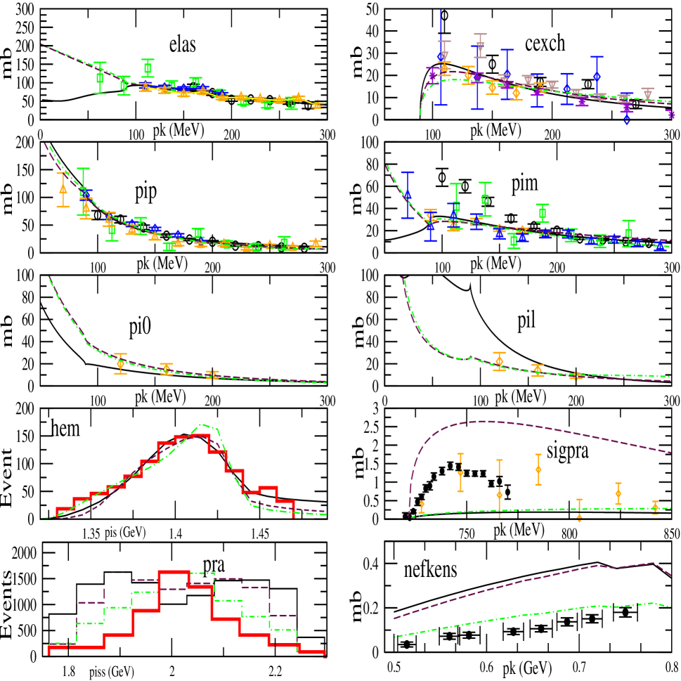
In fig.2 we show the scattering data and the event distributions in the first seven panels, from left to right and top to bottom. The solid and dashed curves, correspond to the and fits, respectively. They reproduce well the data included in the fits of ref.[21] and discussed in this section. The last three panels in the same figure correspond to other data not considered in the present fits nor in ref.[21]. In the eighth panel we show the total cross section . The solid points come from ref.[23] while the diamonds are much older [71]. The event distribution and the total cross section for the reaction , measured in [24], are displayed, respectively, in the ninth and tenth panels. The data in the last three panels will be presented and discussed further in the next section. It is clear from the figure that the and fits do not reproduce adequately the data in the last three panels. In fig.2, we also show by the dash-dotted lines the fit to the same data. As we see, this fit, with 4 free parameters less than the others,#4#4#4We recall that in the fits we also consider , and , directly given by eqs.(3.6) in terms of the low energy constants . In this way, although there are 7 low energy constant only four are really kept as free parameters in the fits. This statement, however, is only approximate because neither nor are exactly sticked to a value, GeV and . is able to reproduce the scattering data but fails as well in the reproduction of , although its disagreement with the data from the reaction [24] is neatly smaller than for the fits and . In table 1 we give the values of the fitted parameters. We show in table 2 the resulting values for the ratios of eq.(3) and observe that for all the fits there is agreement with experiment for and within the small errors given. For , the fits and agree within the experimental error, while agrees with the experimental value at the level of , which is equally satisfactory since we do not intend at this stage to arrive at such precision in the description of strong interactions in this sector, where even isospin breaking corrections should be systematically included. We also show in the same table the kaonic hydrogen data included in the fit, as well as other magnitudes as explained in the table caption. Only the fit is in agreement with the shift and width of kaonic hydrogen from DEAR [1]. The fits and are in agreement with KEK [65] but disagrees with DEAR [1]. We also show the calculated energy shift and width of kaonic hydrogen from the Deser formula. The differences with respect to the results from the more elaborated eq.(3.5) are huge for in the fits and and by far much smaller, a correction of just a few percent, in the fit . For the fit the value for is quite large, although one has to keep in mind that this parameter has very large errors as given by the minimizing subroutine [72]. Indeed, its upper error is much larger than the value of the parameter itself. Hence one concludes that this parameter is left undetermined by the fit. We should also remark that all the parameters in table 1 are of natural size. The are of order GeV-1 and the of around 1. This is the natural size for the since from the value of the imaginary part of above threshold, , multiplying it by , the prefactor in eq.(2.13), one has . Taking for the mass of a nucleon, , the ratio is then the quotient of over MeV, which is typically a quantity of order 1. Furthermore, from the unitarity corrections to the chiral series induced by , which start at , one can derive the scale . Again this scale is of natural size, around the mass of the , for . However, for larger values of it can be quite small, e.g., of the order of the difference between the masses of the nucleon and . Regarding the precise values for , and we can compare our values in table 1 with the determination based on resonance saturation and reproduction of the masses of the lightest baryon octet and from ref.[45]. The authors of ref.[45] conclude that , and in units of GeV-1. From a pure analysis of baryon masses and one has, in the same units, , and or depending on whether the value for is taken from ref.[68] or from ref.[34], respectively. These values look somewhat closer to those of the fit than to the values of the fit . However, the comparison is not straightforward since we employ the couplings in UCHPT, which resums large contributions in this sector, so that there is no reason why the values should be the same as in CHPT. It is remarkable that the value for is very similar both in the fits and . Indeed, from ref.[45] one also has , , and , hence the value for is quite similar also to those in the table. Finally, in ref.[13] a value of around GeV-1 was given as well and in many of the fits of ref.[20] values around GeV-1 are reported. In the fits that we present later, mostly appear between and GeV-1.
| 2.36 | 2.36 | 2.35 | |
| 0.628 | 0.655 | 0.667 | |
| 0.172 | 0.195 | 0.205 | |
| (eV) | 201 | 403 | 390 |
| (eV) | 338 | 477 | 525 |
| (eV) | 209 | 416 | 394 |
| (eV) | 346 | 662 | 716 |
| (fm) | |||
| (fm) | |||
| (fm) | |||
| (∘) | |||
| (GeV) | |||
| () | |||
| (MeV) |
4 New fits with additional recent data
In addition to the data set described in section 3, we now include in the fits the following data, already shown in the last three panels of fig.2:
-
i)
The cross section was measured accurately in ref.[23] from threshold up to around MeV ( GeV), with the kaon three-momentum in the laboratory frame. These are 17 data points with small error bars as shown by the circles in the eighth panel of the result figures, namely, figs.2, 4, 5. We also consider older data on this reaction [71] from up to MeV ( GeV). They are much less precise than the previous data and up to GeV are shown in the eighth panel of the same figures. Both data sets include a total of 29 new points.
-
ii)
Data from the reaction recently measured in ref.[24]. These data comprise the event distribution, shown in the ninth panel of the result figures by the thick solid line, and measurements of the associated total cross section, given by the circles in the tenth panel of the same figures. The measurement of the cross section is quite accurate, as one can see from the figure, with from 0.5 GeV up to 0.75 GeV. The error bars given are calculated from ref.[24] by adding in quadrature the statistical errors (explicitly given in the paper) and a systematic error of (the upper bound estimated in this reference for this source of error). These data constitute 18 demanding new points.#5#5#5I warmly acknowledge E. Oset for having stressed to me the importance of these new data.
-
iii)
Finally, we also include the recently measured difference between the P- and S-wave phase shifts at the mass, from the determination of the decay parameters. The results are [73] and [74]. Neglecting the tiny P-wave phase shift [75], this quantity just corresponds to minus . As already given in ref.[21], we obtain for this quantity for the fit and for the fit . For the fit one has , see table 2. Hence, the fit is the only one in agreement with the measurement at the level of one . In the following we denote by this phase shift difference.
Thus, in total we have 153 “scattering” data points while in ref.[21] the number of “scattering” data points, 97, was significantly smaller.
We follow a similar strategy as in the fits of [21] and then consider fits constrained to give , 30 and 40 MeV. On the other hand, is included in the fits, where the range of values is taken from ref.[69], and is compatible as well with that of ref.[45]. Other works on baryon masses from baryon CHPT, in some or other variant, are [76, 77, 78, 79].
The reaction , accurately measured by the Crystal Ball Collaboration [23], was also considered in refs.[80, 63, 81], where it was assumed to proceed in S-wave. This assumption is well suited since the data from ref.[23] is close to threshold and hence S-wave should dominate, this is also indicated by the angular distributions [23]. We follow here this assumption as well and thus the strong amplitude will be taken in S-wave. According to our normalization we have,
| (4.1) |
as in eq.(3.1), with the CM three momentum of the system and that of the initial state.
For the calculation of the event distribution and the total cross section of the reaction , we follow the scheme of ref.[25], although we use fully relativistic amplitudes. In ref.[25] several production mechanisms for the final state are included and discussed in connection to the related process , studied in ref.[82]. Interestingly, all of them are negligible compared with the diagram shown in fig.3. The thick dot at the right of the figure means that the S-wave is used. Here we are assuming that the process is dominated by the S-wave meson-baryon amplitude, which is justified since we are close to the threshold of the reaction, see the last panel of figs.2, 4 or 5. This diagram is so much enhanced compared with other possible ones [25] due to the almost on-shell character of the intermediate proton. As said above, we have recalculated this diagram in a fully Lorentz covariant way, as also done with the interaction kernel for our S-wave amplitudes. Numerically these relativistic corrections do not affect appreciably the results as compared with the non-relativistic limit taken in ref.[25]. Had the emitted meson been a kaon, things would have been different, since then large factors of would have appeared. The finding of ref.[25], concerning the dominance of the diagram of fig.3 compared with any other considered mechanism, makes us confident about the reliability of the approach and, hence, we include this reaction in our data set.

Our final expression for the reaction is:
| (4.2) | |||||
In the previous equation, and , and are the four-momenta of the incoming proton and outgoing pions, respectively, and is CM energy of the and the second pion. The subscripts and refer to the spins of the proton and , in order. The are Pauli spinors, and , with the proton energy for three-momentum , . The exchange in the end of eq.(4.2) guarantees the indistinguishableness of the two emitted neutral pions. This is the source of a major background for the resonance shape in the event distribution that makes the resonance to appear wider. Taking into account the phase space for the three final particles we have the following expression for the cross section:
| (4.3) |
where is the four-momentum of the , the azimuthal angle of the second pion, the invariant mass of the and the first , while is that of the two pions. The symmetry factor for the calculation of the total cross sections, due to the identical neutral pions, is explicitly shown. In the calculation of the event distribution it should be removed, but since the latter is not normalized we show it for both calculations. Incidentally, we also mention that the S-wave amplitude appearing in eq.(4.2) is evaluated in the -(intermediate ) CM frame, which is not the CM of the whole process, in which is expressed eq.(4.3). We have worked out the corresponding Wigner rotation matrices to calculate the scattering amplitudes in the global CM frame from the S-wave in the -(intermediate ) CM frame. But, since their numerical effects are negligible, we refrain from including them and giving further details about their calculation.
4.1 New type fits
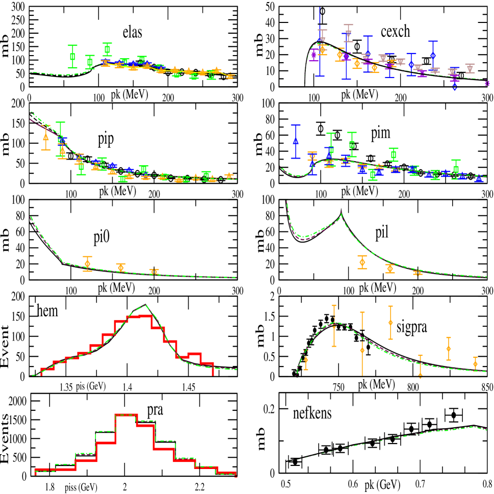
We first discuss those fits that reproduce the DEAR accurate measurement, eq.(3.4), of the width and shift of kaonic hydrogen, together with the rest of data. We show in fig.4 the reproduction of the scattering data for these new fits, that include the additional data discussed in this section. We distinguish the fits according to the enforced value introduced in the fit and calculated from eq.(3.6). These values, in MeV, are (solid), (dashed) and (dash-dotted lines). These fits, once the new data is included, originate from the one, and many fitted values of the parameters, shown in table 3, are quite similar to those of given in table 1. The main difference is the value for concerning the channel, that is much smaller now than it was in table 1. The value for is also a few MeV smaller now than for . We have also tested another fit with MeV, taking for the central value from ref.[68] and adding linearly the error given in this reference and the expected uncertainties from higher orders [67]. Nonetheless, the resulting fit is somehow intermediate between the fits with and and we do not consider it any further. We obtain a good reproduction of the scattering data as shown in fig.4. Although the different lines in this figure can be barely distinguishable, we show the different fits separately in table 3 to illustrate how different fits can give rather similar results. The main differences in the outputs, as shown in table 4, come from the values of and, of course, of the enforced . In addition, we also give in this table several other observables as in table 2. For the ratio , the values given in table 3 agree with the experiment, eq.(3), within , like in the case of . It is worth stressing the perfect agreement with DEAR, concerning the energy shift and width for kaonic hydrogen, for all the fits of table 3, while, at the same time, all the scattering data shown in fig.4, plus , , and , are reproduced too.
The scattering lengths shown in the previous table are similar to those of the fit in table 2. Of course, they are much smaller in absolute value than those of fits and . This is related to the fact that the new fits, as , reproduce the DEAR data which, by the Deser formula, requires a much smaller scattering length than those of the fits and . Let us recall that the fit of ref.[21] was the first chiral fit to be in agreement with the recent and accurate kaonic hydrogen data from ref.[1] and the scattering data of section 3. Nonetheless, since the fits in table 3 are also able to provide a good reproduction of the new precise data from refs.[23, 24], they are preferred by us over the one.
It is remarkable as well the agreement with the measurement of from refs.[73, 74]. The values in table 4 are considerably larger than those obtained in ref.[83] from an analysis using UCHPT, where the range was determined from an analysis of the scattering data of section 3. Hence we see that the effect of the higher orders in the kernel are quite relevant for a precise determination of this quantity.
| Units | ||||
|---|---|---|---|---|
| MeV | ||||
| MeV | ||||
| GeV-1 | ||||
| GeV-1 | ||||
| GeV-1 | ||||
| GeV-1 | ||||
| GeV-1 | ||||
| GeV-1 | ||||
| GeV-1 | ||||
| 2.36 | 2.36 | 2.37 | |
| 0.629 | 0.628 | 0.628 | |
| 0.168 | 0.171 | 0.173 | |
| (eV) | 194 | 192 | 192 |
| (eV) | 324 | 302 | 270 |
| (eV) | 204 | 204 | 207 |
| (eV) | 361 | 338 | 305 |
| (fm) | |||
| (fm) | |||
| (fm) | |||
| (∘) | 3.4 | 4.5 | 5.7 |
| (GeV) | 1.2 | 1.1 | 1.0 |
| () |
4.2 New type fits
| Units | |||||
|---|---|---|---|---|---|
| MeV | |||||
| MeV | 93.9 | ||||
| GeV-1 | |||||
| GeV-1 | |||||
| GeV-1 | |||||
| GeV-1 | |||||
| GeV-1 | |||||
| GeV-1 | |||||
| GeV-1 | |||||
| 2.34 | 2.35 | 2.34 | 2.32 | |
| 0.643 | 0.643 | 0.644 | 0.637 | |
| 0.160 | 0.163 | 0.176 | 0.193 | |
| (eV) | 436 | 409 | 450 | 348 |
| (eV) | 614 | 681 | 591 | 611 |
| (eV) | 418 | 385 | 436 | 325 |
| (eV) | 848 | 880 | 844 | 775 |
| (fm) | ||||
| (fm) | ||||
| (fm) | ||||
| (∘) | 1.7 | |||
| (GeV) | 0.8 | 0.6 | 0.7 | … |
| () | … |
Now, we report about other fits to the whole set of data that originate from the fit of ref.[21]. We also include here an fit to all the data of this section, except for the magnitudes in eq.(3.6), as they are defined in terms of the couplings. Following the same scheme of presentation as in the prior subsection, we enforce in the fits that , or MeV. The fitted parameters are given in table 5, while the results are shown in table 6 and in fig.5 by the solid (), dashed () and dash-dotted lines (). The new fit is given in the last column of table 5 and its results are given in the last column of table 6 and in fig.5 by the dotted lines.
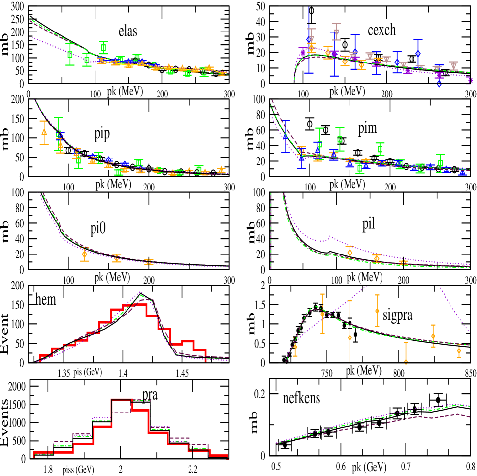
We observe that all the fits in table 5 reproduce very well the scattering data, except for the fit which badly fails in the reproduction of , shown in the eighth panel. However, all these fits strongly disagree with the DEAR measurement, eq.(3.4), of the energy shift and width of the kaonic hydrogen, particularly for the former. It is also worth noticing that for the fits in table 5 the corrections of eq.(3.5) over the Deser formula for are large, around a , see table 6, much larger than for the fits of table 3. In addition, the fits , and are also around 3 sigmas below the value of measured in ref.[73]. For the fit the disagreement is at the level of 2 sigmas. All this seems to indicate that the fits of table 3 give a better overall reproduction of the data on scattering than those in table 5. Of course, the hypothetical confirmation of the DEAR data on the energy shift and width of kaonic hydrogen by the DEAR/SIDDHARTA Collaboration [2] will certainly refute the fits in table 5.
5 Spectroscopy
In this section we discuss in detail the pole content of our main fit, the third one in table 3. This fit will be referred in the following as I. We also present more briefly those poles corresponding to the and fits of table 5. The former will be called in the subsequent as II. Those other fits in tables 3 and 5 have a pole content very similar to that of the considered fits, I and II, respectively, and hence, we will not discuss them separately for the sake of brevity.
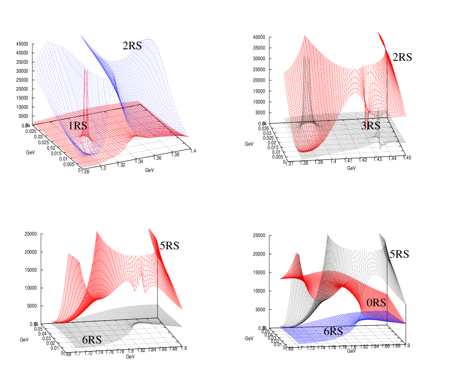
We only consider those Riemann sheets that are connected continuously to the physical sheet in some energy region of the physical axis. The physical Riemann sheet is such that the imaginary part of the modulus of the three-momentum associated with every channel is positive. The other Riemann sheets are defined depending on which three-momenta are evaluated in the other sheet of the square root, with an additional minus sign. The first non-physical Riemann sheet, 1RS, is reached when crossing the physical axis between the thresholds of and , from 1.25 to 1.33 GeV, approximately.#6#6#6In the definition of the sheets we just talk about the , or thresholds, although in the physical case, because of isospin violation, these “thresholds” indeed refer to a narrow region, less than 10 MeV wide at most. The so called second sheet, 2RS, is reached when crossing the physical axis between the thresholds of and , around 1.34 and 1.43 GeV, respectively. The third sheet, 3RS, is connected continuously to the physical sheet between the thresholds of and , 1.44 and 1.66 GeV, approximately. The fourth sheet, 4RS, can be reached when crossing the physical axis between the and thresholds, from around 1.66 to 1.74 GeV. The fifth sheet, 5RS, is connected to the physical one between the thresholds of and , around 1.74 and 1.81 GeV, respectively. And finally, the sixth sheet, 6RS, is reached by crossing the physical axis above the threshold, approximately at 1.81 GeV. In all the sheets, NRS, one has , for , and for . (For one must understand that all the three-momenta have negative imaginary part.)
Once the pole position is known, one can then calculate the couplings by performing the limit,
| (5.1) |
with the pole position for the s Mandelstam variable. The is the coupling of the pole to the channel .
| Re(Pole) | -Im(Pole) | Sheet | |||||||
|---|---|---|---|---|---|---|---|---|---|
| 1301 | 13 | 1RS | |||||||
| 0.03 | 1.12 | 0.02 | 0.01 | 5.83 | 0.05 | 0.41 | 0.04 | 2.11 | 0.03 |
| 1309 | 13 | 2RS | |||||||
| 0.02 | 3.66 | 0.02 | 0.02 | 4.46 | 0.04 | 0.21 | 0.04 | 3.05 | 0.03 |
| 1414 | 23 | 2RS | |||||||
| 0.14 | 4.24 | 0.13 | 0.01 | 4.87 | 0.39 | 0.85 | 0.20 | 9.35 | 0.11 |
| 1388 | 17 | 3RS | |||||||
| 0.02 | 3.81 | 0.02 | 0.02 | 1.33 | 0.04 | 0.42 | 0.04 | 9.55 | 0.04 |
| 1676 | 10 | 3RS | |||||||
| 0.01 | 1.28 | 0.03 | 0.00 | 1.67 | 0.01 | 2.19 | 0.07 | 5.29 | 0.07 |
| 1673 | 18 | 4RS | |||||||
| 0.01 | 1.26 | 0.02 | 0.00 | 1.82 | 0.01 | 2.13 | 0.06 | 5.32 | 0.06 |
| 1825 | 49 | 5RS | |||||||
| 0.02 | 2.29 | 0.02 | 0.00 | 2.10 | 0.02 | 0.89 | 0.03 | 7.43 | 0.09 |
5.1 Fit I
-
•
I=0 Poles: There are two I=0 poles very close to the threshold, one in the 1RS and the other in the 2RS sheet. They are located at and MeV, for the sheets 1RS and 2RS, respectively. The first pole has a small coupling#7#7#7All couplings will be given in GeV. 1.12 to , while this coupling is large for the second pole, 3.68. This makes that the bump in the square of the I=0 amplitude is very asymmetric around the threshold. On the left of this threshold one has the behaviour corresponding to 1RS, so that one observes basically a cusp effect with very little influence of the 1RS pole, while at the right of the threshold the behaviour is dominated by the falling at the right of the 2RS pole. This is illustrated in the first panel of fig.6, from left to right and top to bottom, where the square modulus of the I=0 S-wave is shown. These two poles reflect the same resonance because they are connected continuously when passing softly via a continuous parameter from the 1RS to the 2RS, as we have checked. For the channel one has a peak at the 1RS pole position, although the opening of the channel makes a strong cusp effect that distorts strongly the resonance shape giving rise to a sharp dip between the thresholds along the right tail of the 2RS pole. On the 2RS we also have another pole at MeV, with large couplings to (4.24), (4.87) and (9.35). Note that all the ten coupled channels are degenerate in the SU(3) limit and hence SU(3), simply because of the Wigner-Eckart theorem, does permit large couplings of a resonance to much heavier channels than the resonance mass. This pole, 2RS 1414, gives rise to the “standard” resonance, clearly seen in the event distribution of figs. 2, 4 and 5. Its width resulting from the pole position#8#8#8As it is well known, minus twice the imaginary part of the pole position is the width of the resonance. Nonetheless, this is only so when the resonance is narrow and its difference to the closest threshold is substantially larger than the width. is around 46 MeV. Their parameters, mass and width, are then in good agreement with those of the PDG [61]. The right most shape of this resonance, above the thresholds, does not correspond to any pole in the 3RS plane and just corresponds to a cusp effect due to the opening of the thresholds. This behaviour is shown in the second panel of fig.6, where the square modulus of the I=0 S-wave is plotted. In this panel one can also observe a narrow pole between the and thresholds corresponding to a narrow I=1 pole to be discussed below. This pole appears in I=0 because of isospin violation. In the 3RS we find another pole at MeV that controls, modulo the cusp effect at the opening of the thresholds, the size of the I=0 amplitudes. This pole couples much more weakly to , and this is why it does not affect its shape in the physical sheet, see the second panel. These two latter poles, 2RS 1414 and 3RS 1388, are connected continuously and, hence, reflect the same resonance, the . As discussed above, before this resonance we also have another one, peaked around the threshold. In ref.[18] the fact of having two nearby poles around the nominal mass of the was referred as the dynamics of the two . In our solution we still find two resonances, but one of these “” has moved to lower energies, and the two peaks can be distinguished now. We now consider the resonance [61], this is clearly visible in the ref.[23] data on the reaction , as shown in the eighth panel of figs. 2, 4 and 5. The left part of this resonance, before the opening of the threshold, is driven by the pole in the 3RS at MeV, while the right part, above the threshold, is driven by the pole in the 4RS at MeV. Both poles have similar values for mass and width although they are not the same, which is specially relevant in this case since the width is rather small, around 20 MeV, and because of the nearby position of the threshold. These poles have their largest couplings to the and channels, around 2.1 and 5.3, respectively. We also warn that the actual shape of the resonance can depend strongly on the process. For example, for the square modulus of the or elastic I=0 scattering amplitudes, the peak is shifted to higher energies, towards 1.7 GeV, because of a strong distortion induced in these cases by the channel. For this channel the appears as a clean strong enhancement. However, its shape is an asymmetric distorted Breit-Wigner resonance because on the left of the threshold it has a width of around 20 MeV, from the 2RS 1676 pole, while on the right its width is larger, around 26 MeV, from the 4RS 1673 pole. The poles 3RS 1676 and 4RS 1673 are connected continuously, as one would expect. They reflect, as discussed, the resonance. In the 5RS there is another pole at MeV. This pole drives an increase in the I=0 amplitudes involving the , and I=0 states to which it couples strongly, 2.3, 2.1 and 7.4, respectively, for a few tens of MeV before the threshold. The coupling to is much weaker, 0.9, and it does not give rise to any rapid movement for this case. This pole disappears in the 6RS, and for energies higher than the threshold one only has a remarkable cusp effect. This is accompanied by an important decrease in the values of the I=0 amplitudes for those to which the previous pole strongly couples. See the third panel of fig.6, where the square modulus of the elastic I=0 S-wave is shown. In the PDG [61] there is an entry for the resonance with values for its mass and width in correspondence with the pole position just given. However, we must stress that its signal in any scattering amplitude is far from being that of a simple Breit-Wigner because it appears just on top of the threshold (the distance to that is much smaller than its width of around 100 MeV), and this pole appears in one sheet but not in the next one. E.g., its value for the width as minus twice the imaginary part of the pole position is not appropriate for this case to the right of the threshold. In the last panel of fig.6 we show the square modulus of the same amplitude as in the third panel but now, in addition, we also show the physical sheet, indicated by 0RS. It is remarkable how this sheet matches along the real axis, because of continuity, first to the 5RS and then, after the threshold, to the 6RS. To show this more clearly, we have plotted the amplitude in the isospin limit for this last panel, so that only one threshold is present. We give in table 7 the pole positions and couplings of the discussed I=0 poles.
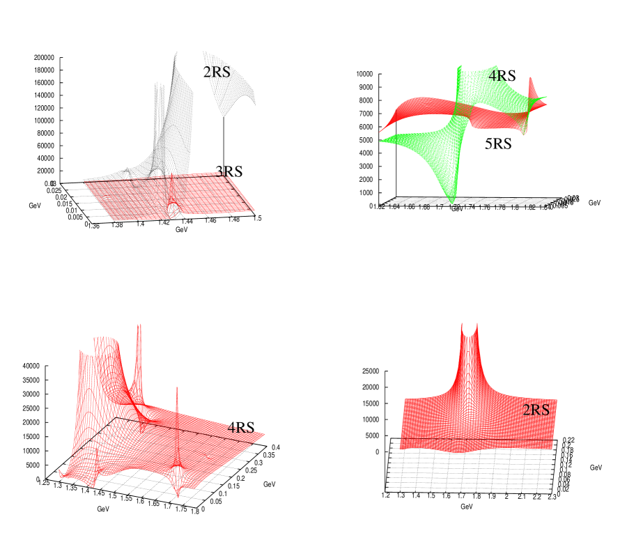
Figure 7: Some poles with I=1 for the fit I. From left to right and top to bottom, we have the square modulus of the I=1 S-waves: , and again of . The last panel corresponds to the square modulus of the I=2 S-wave. Re(Pole) -Im(Pole) Sheet 1425 6.5 2RS 1.35 0.24 1.66 0.01 0.35 3.92 0.05 4.23 0.49 2.98 1468 13 2RS 2.80 0.16 5.96 0.02 0.23 8.74 0.04 10.66 0.19 2.48 1433 3.7 3RS 0.65 0.08 0.80 0.00 0.12 1.58 0.02 5.82 0.20 2.14 1720 18 4RS 1.82 0.02 1.21 0.00 0.02 0.95 0.02 6.78 0.05 5.31 1769 96 6RS 2.65 0.00 0.61 0.00 0.00 2.48 0.00 3.32 0.01 4.22 1340 143 3-4RS 1.33 0.14 5.50 0.02 0.02 1.58 0.00 3.28 0.03 1.20 1395 311 3-4RS 2.08 0.01 1.49 0.01 0.00 1.24 0.00 7.63 0.01 3.97 Table 8: Fit I, I=1 Poles. The pole positions are given in MeV and the couplings in GeV. The couplings to the I=0, 2 channels are always close to zero. -
•
I=1 Poles: In the 2RS we find two narrow I=1 poles close to the thresholds. One located at MeV and the other at MeV. The first one has a coupling of 1.7 while the other has a much stronger coupling of 6.0. They interfere destructively around 1.42 GeV and there is a dip there, as shown in the first panel of fig.7, where the square modulus of the elastic I=1 S-wave is plotted. Indeed, this is the only observable signal in the square of the I=1 elastic amplitude for the second pole, because it disappears in the 3RS. Had the heavier pole not appeared we would then have obtained a symmetric and standard Breit-Wigner resonance shape for the pole at MeV. Instead, we find a sharp dip to the right of the pole position. This remarkable destructive interference for the and I=1 amplitudes below the threshold is due to the large couplings of the pole in the 2RS at MeV to (6.0) and (8.7). This effect is not so strong in the case because its coupling is smaller, 2.8. The 2RS pole MeV evolves continuously in the 3RS to another pole at MeV. This pole drives the behaviour of the I=1 amplitudes at the right of the threshold. These two poles, being connected, correspond to the same resonance. We see then that the behaviour of the I=1 amplitudes from around 1.4 up to 1.45 GeV is dominated by these three poles, giving rise to a pronounced peak structure in the amplitudes. Recently, a signal for a resonance at MeV and width of MeV has been reported from the reaction in ref.[62]. Maybe, one can invoke interference effects to account for the displacement of our peak around 1.43 GeV to somewhat higher energies, as observed by COSY. Other relevant pole for the I=1 amplitudes is the one located at MeV on the 4RS. This pole is visible like a distorted bump in the (1.82), (1.21) and (0.95) S-waves, however is a clean resonance signal for the not yet open (6.78) and (5.31) channels. In the 5RS this pole disappears and one only observes a cusp effect in some channels whose value matches with the descending tail of the former pole in the 4RS. This enhancement corresponds to the resonance of the PDG, in good agreement with its values of mass and width. We show this behaviour in the second panel of fig.7 by plotting the square modulus of the S-wave. In the 6RS sheet we find a relevant pole at MeV, with a width of around 200 MeV, which is responsible for the size and the slow descending value of the I=1 amplitudes after the cusp around the thresholds. Hence, this pole cannot be observed directly as a bump in the physical axis. Regarding the [61], some of the I=1 S-wave amplitudes show a broad bump after the threshold and before that of the . These bumps, like the one shown in the second panel of fig.7 for the 5RS surface of the elastic amplitude, is due to the interference of multiple poles. Two of them have been already discussed, namely, the 3RS 1433 and 4RS 1720 poles. In addition, there are other two broad poles at and MeV, shown in the last two lines of table 8, that appear simultaneously in the 3RS and 4RS in the same positions#9#9#9Notice that the channel is I=0 and this is why it does not appreciably modify the pole positions of these broad I=1 poles.. These poles, because of their long descending tails, control to a large extent the sizes of the I=1 amplitudes in this region . All this produces this interesting interference phenomenon of soft bumps on the physical axis as shown in the panel before the last one of fig.7. In this panel the square modulus of the elastic I=1 S-wave is drawn. For this case, the wider pole is not very relevant, however, it is so for the channel because its coupling to this channel is much larger than that of the lighter resonance at 1340 MeV. This is why we have kept it. The pole MeV on the 3RS or 4RS sheets is connected continuously to the previous 2RS pole at MeV, hence, for this solution, the and are clearly related. In table 8 we collect the different I=1 poles for the fit I presented here.
-
•
I=2 Pole: An exotic I=2 pole appears at MeV with a strong coupling to the I=2 channel (the only one possible with I=2) of 6.18. This pole appears in the 2RS, 3RS, 4RS, 5RS and 6RS, since in all of them the momentum for the has reversed sign and the only channel that matters is the I=2 . This pole is actually the responsible for the I=2 size and gives rise to a soft and wide bump in the square modulus of the I=2 amplitude, with a dip at 1.7 GeV due to a zero, see the last panel of fig.6, where the square of the modulus of the I=2 S-wave is shown. Because of this non uniform shape and for its rather large magnitude, of the same order as that for the other isospin channels, one can think of the possibility of detecting such exotic state.
5.2 Fits II and
We consider here the pole content of the fits II and , both fits are given in table 5. Tables 9 and 10 correspond to the I=0, 1 poles of fit II, while the tables 11 and 12 are the same for the fit.
| Re(Pole) | -Im(Pole) | Sheet | |||||||
|---|---|---|---|---|---|---|---|---|---|
| 1347 | 36 | 2RS | |||||||
| 0.02 | 6.48 | 0.12 | 0.02 | 2.60 | 0.10 | 1.42 | 0.01 | 0.32 | 0.07 |
| 1427 | 18 | 2RS | |||||||
| 0.12 | 3.87 | 0.23 | 0.01 | 6.99 | 0.23 | 3.49 | 0.05 | 1.64 | 0.32 |
| 1340 | 41 | 3RS | |||||||
| 0.07 | 5.92 | 0.08 | 0.01 | 0.62 | 0.08 | 2.33 | 0.01 | 0.75 | 0.04 |
| 1667 | 8 | 4RS | |||||||
| 0.03 | 0.77 | 0.05 | 0.00 | 0.59 | 0.01 | 3.32 | 0.02 | 12.17 | 0.08 |
| 1667 | 8 | 5RS | |||||||
| 0.03 | 0.77 | 0.05 | 0.00 | 0.59 | 0.01 | 3.32 | 0.03 | 12.17 | 0.06 |
For the I=0 poles of fit II we observe that the region is controlled by three poles, two in the 2RS and one in the 3RS. The first two control the shape before the threshold and the latter after this threshold is open. The 2RS 1347 and 3RS 1340 poles couple very strongly to while the 2RS 1427 pole couples very strongly to . Hence, the resonance looks broader for the channel than for the , since the resonance for the former mostly corresponds to the broader poles while for the latter it is mainly due to the narrower one. As a further consequence, for the resonance peak is shifted to the right. This kind of behaviour is already described in detail in ref.[18], where analyses were used. In addition, the two poles 2RS 1347 and 3RS 1340 are connected when passing continuously from the 2RS to the 3RS. The resonance is described by the two poles located in the same place both in the 4RS and 5RS, giving rise to a clean symmetric Breit-Wigner without asymmetries in the threshold. Of course, these two poles are continuously connected. There is no signal for the .
| Re(Pole) | -Im(Pole) | Sheet | |||||||
|---|---|---|---|---|---|---|---|---|---|
| 1399 | 41 | 2RS | |||||||
| 1.49 | 0.09 | 5.58 | 0.01 | 0.13 | 4.92 | 0.08 | 0.73 | 0.03 | 4.99 |
| 1424 | 3.6 | 2RS | |||||||
| 0.54 | 0.14 | 1.58 | 0.00 | 0.20 | 1.17 | 0.10 | 0.61 | 0.04 | 3.76 |
| 1311 | 122 | 3-4RS | |||||||
| 2.63 | 0.05 | 4.61 | 0.01 | 0.02 | 3.44 | 0.02 | 0.60 | 0.03 | 3.60 |
| 1426 | 3 | 3RS | |||||||
| 0.56 | 0.04 | 1.18 | 0.00 | 0.07 | 0.77 | 0.04 | 0.61 | 0.02 | 3.74 |
We now turn to the I=1 poles for fit II. The region below the threshold is governed by the 2RS poles at and MeV. The latter appears as a dip in the slope of the former since the interference is destructive. Above the threshold one has again two poles, one broad and the other narrow, located in the 3RS at and MeV, respectively. In this case, the latter appears as a clear peak in the slope of the former. The 2RS 1399 and 3RS 1311 poles are connected continuously and then corresponds to the same resonance. The same happens for the 2RS 1424 and 3RS 1426 poles, as one would expect. All these poles give rise to a broad enhancement of the I=1 S-waves up to around 1.45 GeV. We do not observe any signal for the . Regarding the , a few amplitudes, like that of , exhibits an enhancement around 1.6 GeV. Nonetheless, there is no a clear pole structure driving this behaviour. The most remarkable facts are the presence of a broad pole on the 3-4RS at MeV, which controls, up to some extent, the size of the amplitudes in this region through its falling tail, and the opening of the channel, that always produce a pronounced cusp effect, sometimes like a bump others like a dip. Nonetheless, for fit I there were more amplitudes manifesting bumps around 1.6 than now for fit II.
| Re(Pole) | -Im(Pole) | Sheet | |||||||
|---|---|---|---|---|---|---|---|---|---|
| 1375 | 60 | 2RS | |||||||
| 0.04 | 7.55 | 0.07 | 0.02 | 5.45 | 0.07 | 2.20 | 0.02 | 0.78 | 0.07 |
| 1429 | 22 | 2RS | |||||||
| 0.13 | 4.68 | 0.14 | 0.01 | 6.85 | 0.21 | 4.50 | 0.20 | 0.54 | 0.17 |
| 1710 | 19 | 4RS | |||||||
| 0.05 | 0.27 | 0.03 | 0.00 | 1.73 | 0.03 | 2.56 | 0.05 | 10.75 | 0.09 |
| 1710 | 19 | 5RS | |||||||
| 0.04 | 0.27 | 0.04 | 0.00 | 1.73 | 0.05 | 2.56 | 0.04 | 10.75 | 0.11 |
We now consider the fit. The first I=0 pole occurs at MeV on the 2RS with a large coupling to . This pole interferes destructively with that at MeV and this is why, at this point, the elastic I=0 S-wave has a dip. The latter pole couples very strongly with and it is seen as a clear maximum in the partial wave. There is no pole at around 1.4 GeV in the 3RS sheet and the right tail of this resonance, after the threshold, corresponds to a pronounced cusp effect that falls down from the latter threshold. Thus, for all the fits I, II and we observe the presence of a minimum in the I=0 amplitudes before 1.42 GeV, a maximum for the modulus of the I=0 S-wave before such energy (for the fits I, II and the maximum is located around 1.34, 1.36 and 1.38, in order), and a maximum for the amplitudes involving the channel around its threshold. As discussed before, this is related to the so called dynamics of the two [18]. The region is given by the poles 4RS and 5RS 1710, which have very similar properties and are continuously connected when passing from one sheet to the other. These poles describe this resonance above and below the threshold, respectively. There is no signal for the .
| Re(Pole) | -Im(Pole) | Sheet | |||||||
|---|---|---|---|---|---|---|---|---|---|
| 1423 | 1.3 | 2RS | |||||||
| 0.52 | 0.12 | 0.72 | 0.00 | 0.18 | 1.28 | 0.11 | 1.49 | 0.02 | 2.30 |
| 1494 | 116 | 2RS | |||||||
| 3.83 | 0.15 | 10.06 | 0.03 | 0.14 | 9.25 | 0.06 | 2.82 | 0.02 | 4.55 |
| 1425 | 4.8 | 3RS | |||||||
| 0.93 | 0.05 | 1.22 | 0.00 | 0.11 | 1.63 | 0.07 | 2.71 | 0.01 | 3.43 |
| 1796 | 69 | 4RS | |||||||
| 3.97 | 0.01 | 2.33 | 0.01 | 0.02 | 1.96 | 0.03 | 3.20 | 0.15 | 9.09 |
| 1808 | 71 | 5RS | |||||||
| 3.71 | 0.01 | 1.94 | 0.00 | 0.01 | 2.36 | 0.02 | 1.15 | 0.11 | 8.16 |
| 1350 | 254 | 3-4RS | |||||||
| 2.38 | 0.06 | 5.19 | 0.01 | 0.02 | 3.36 | 0.01 | 5.33 | 0.01 | 4.11 |
The narrow I=1 pole 2RS 1423 only has an appreciable coupling to the channel, closed at such energies, and this is why it is so narrow. This pole appears as a dip in the increasing slope of the wide 2RS 1494 pole. In the 3RS one has another pole at MeV, continuously connected to the 2RS 1423 one. As in fits I and II, all these poles give rise to a clear resonance structure up to around 1.5 GeV, close to the nominal mass of the resonance, and overlapping when taking into account widths [61]. In addition, the enhancement corresponding to the [61] appears again in this fit, as in fit I, and it corresponds to the relatively wide 4RS and 5RS MeV poles, in the relevant sheets for energies below and above the threshold, respectively. These two poles are connected continuously. The bumps disappear for this fit. Although one has the mentioned resonances around the and thresholds, the amplitudes do not display bumps between them. One also has in the 3-4RS a wide pole at MeV that interferes appreciably in the physical axis with the previous resonances but, in this case, this interference is negative, while in the fit I was positive. This pole is continuously connected to the 2RS 1494 pole.
We want to end this section with some SU(3) considerations. Without moving to the SU(3) limit, we calculate the interaction kernels, , appearing in eq.(2.12), for the SU(3) irreducible representation , , , , and . These are the ones that originate from the tensorial product of the octets of baryons and mesons. If one performs such an exercise, one realizes that for the fit I the , , and have attractive kernels. These representations can accommodate four I=0 and three I=1 resonances, in agreement with the resonance content discussed above. For the fit II, one obtains attraction in the representations , , and . In this case, the previous SU(3) representations can accommodate three I=0 and 1 resonances, although only two I=1 resonances finally appear. Similarly, for the fit one has attractive interaction in the representations , , and . As before these representations can accommodate three I=0 and 1 resonances. This is in agreement with the fact that any of the latter two fits does not reproduce the resonance, while this is the case for the fit I.
6 Conclusions
We have considered a wide set of experimental data that includes several cross sections, namely, the elastic and charge exchange ones and productions of hyperons (, , and ), the event distribution from ref.[60], the reaction from ref.[24], including a event distribution and the total cross section, the total cross section of [23], three ratios , and of cross sections at the threshold of [58, 59], the difference of the P- and S-wave phase shifts at the mass [73, 74], , and the three quantities, , , , calculated at in baryon CHPT. Last, but not least, we have paid special attention to the energy shift and width of the line () of kaonic hydrogen in connection to its recent and accurate measurement by the DEAR Collaboration [1]. We have reviewed the fits of ref.[21], including as well a new fit, and shown that they cannot reproduce the additional data considered in section 4, that is, those from [24] and from [23]. These fits are given in table 1. We have then searched for new fits including from the beginning all the previous set of data points. Several fits arise, namely, the ones given in tables 3 and 5, that reproduce most of the data. The only exceptions are and the DEAR data, eq.(3.4), that are not in agreement (within the present precision given by their last measurements from refs.[73] and [1], respectively) with the fits of table 5. The fit given in that table does not reproduce in addition the total cross section. Remarkably, the fits of table 3 are able to reproduce the whole set of data and, taking into account the value for , around 50 MeV [68, 34], we consider as our main fit, the so called fit I, the last one in this table with MeV. Nonetheless, all of them give very similar results for the rest of quantities, as shown in fig.4. Indeed, the values of the fitted free parameters are very similar, as shown in table 3. The values of the parameters of our main fit are quite similar to those of the fit of ref.[21] as well. This was the first fit to provide a set of chiral parameters leading to a simultaneous reproduction of the scattering data considered in ref.[21] and the DEAR value on the width and shift of kaonic hydrogen. In addition, we have analysed in detail the pole content of the fits I (main fit), II (the fit of table 5), and from table 5. We have discussed with special care the pole content of fit I and shown how it reproduces the two resonances, and the , , , and resonances, as called in the PDG. We have shown that there is no a one to one correspondence between poles and resonances and that the pole structure of a resonance can indeed be very involved, particularly, as it is always the case here, when there is a threshold in the nearby. One then must consider in detail the connection between Riemann sheets, in order to disentangle which poles are responsible for such effects, and collect as the same resonance those poles that are connected when passing continuously from one sheet to the other. Regarding the pole contents of fits II and , the former does not contain any poles associated with the and the resonances, while the latter does not reproduce the nor the bumps. Finally, fit I gives rise to an exotic broad I=2 resonance that could be observed since its size is similar to that of the other isospin S-waves, its shape is non-uniform and is the only resonance present in I=2. Thus, also from the point of view of spectroscopy, the fit I is the solution that fits better with the present resonance content in S-wave strangeness as given in the PDG [61], giving rise to all the strangeness S-wave resonances from the onset of the channel up to energies above 1.8 GeV. We then conclude that fit I is our preferred fit in view of its unique agreement with the scattering, atomic and spectroscopic experimental information.
Acknowledgements
I would like to acknowledge fruitful common work and discussions with my collaborators J. Prades and M. Verbeni. I also thank E. Oset for useful discussions and communications. Financial support by MEC (Spain) grant No. FPA2004-03470, the European Commission (EC) RTN Program Network “EURIDICE” Contract No HPRN-CT-2002-00311 and the HadronPhysics I3 Project (EC) Contract No RII3-CT-2004-506078 is acknowledged.
References
- [1] G. Beer et al. [DEAR Collaboration], Measurement of the kaonic hydrogen X-ray spectrum, Phys. Rev. Lett. 94, 212302 (2005).
-
[2]
D. L. Sirghi and F. Sirghi, (DEAR/SIDDHARTA Collaboration),
The physics of kaonic atoms at DAFNE,
http://www.lnf.infn.it/esperimenti/dear/DEAR_RPR.pdf
C. Curceanu (DEAR/SIDDHARTA Collaboration), Precision measurements of kaonic atoms at DAFNE,
www.tp2.ruhr-uni-bochum.de/vortraege/workshops/trento05/Petrascu.pdf - [3] U.-G. Meißner, U. Raha and A. Rusetsky, Spectrum and decays of kaonic hydrogen, Eur. Phys. J. C35, 349 (2004).
- [4] S. Deser et al., Energy level displacements in mesonic atoms, Phys. Rev. 96, 774 (1954); T. L. Trueman, Energy level shifts in atomic states of strongly-interacting particles, Nucl. Phys. 26, 57 (1961).
- [5] R. H. Dalitz and S. F. Tuan, Possible resonant state in pion-hyperon scattering, Phys. Rev. Lett. 2, 425 (1959); The energy dependence of low energy processes, Ann. Phys. 8, 100 (1959).
- [6] A. D. Martin, N. M. Queen and G. Violini, Consistency tests of the low-energy parametrizations, Nucl. Phys. B10, 481 (1969); P. M. Gensini, R. Hurtado and G. Violini, phenomenology from anti- scattering, PiN Newslett. 13, 291 (1997). [arXiv:nucl-th/9709023]; B. Di Claudio, A. M. Rodriguez-Vargas and G. Violini, The Adler-Weisberger sum rule and the sigma commutator for the kaon-proton system, Z. Phys. C3, 75 (1979).
- [7] A. D. Martin, Kaon-nucleon parameters, Nucl. Phys. B179, 33 (1979).
- [8] R. Buttgen, K. Holinde and J. Speth, scattering and meson exchange, Phys. Lett. B163, 305 (1985); R. Buettgen, K. Holinde, A. Mueller-Groeling, J. Speth and P. Wyborny, A meson exchange model for the interaction, Nucl. Phys. A506, 586 (1990); A. Mueller-Groeling, K. Holinde and J. Speth, interaction in the meson exchange framework, Nucl. Phys. A513, 557 (1990).
- [9] T. Hamaie, M. Arima and K. Masutani, Negative-parity hyperons in the constituent quark model with meson-quark couplings, Nucl. Phys. A591, 675 (1995)
- [10] P. J. Fink, G. He, R. H. Landau and J. W. Schnick, Bound states, resonances and poles in low-energy anti- interaction models, Phys. Rev. C41, 2720 (1990).
- [11] E. A. Veit, B. K. Jennings, R. C. Barrett and A. W. Thomas, Kaon-nucleon scattering in an extended cloudy bag model, Phys. Lett. B 137, 415 (1984).
- [12] J. L. Goity, C. L. Schat and N. N. Scoccola, Negative parity 70-plet baryon masses in the expansion, Phys. Rev. D66, 114014 (2002); Masses of the baryons in large QCD, Phys. Rev. Lett. 88, 102002 (2002).
- [13] N. Kaiser, P. B. Siegel and W. Weise, Chiral dynamics and the low-energy kaon-nucleon interaction, Nucl. Phys. A594, 325 (1995).
- [14] J. A. Oller and E. Oset, Chiral symmetry amplitudes in the S-wave isoscalar and isovector channels and the , , scalar mesons, Nucl. Phys. A620, 438 (1997); (E)-ibid. A652, 407 (1999).
- [15] E. Oset and A. Ramos, Non perturbative chiral approach to s-wave anti- interactions, Nucl. Phys. A635, 99 (1998).
- [16] J. A. Oller, E. Oset and A. Ramos, Chiral unitary approach to meson-meson and meson-baryon interactions and nuclear applications, Prog. Part. Nucl. Phys. 45, 157 (2000).
- [17] J. A. Oller and U.-G. Meißner, Chiral dynamics in the presence of bound states: kaon-nucleon interactions revisited, Phys. Lett. B500, 263 (2000).
- [18] D. Jido, J. A. Oller, E. Oset, A. Ramos and U.-G. Meißner, Chiral dynamics of the two states, Nucl. Phys. A725, 181 (2003).
- [19] C. Garcia-Recio, M. F. M. Lutz and J. Nieves, Quark mass dependence of s-wave baryon resonances, Phys. Lett. B582, 49 (2004).
- [20] B. Borasoy, R. Nissler and W. Weise, Kaonic hydrogen and scattering, Phys. Rev. Lett. 94, 213401 (2005); Chiral dynamics of kaon nucleon interactions, revisited, Eur. Phys. J. A25, 79 (2005); Comment on ‘Surprises in threshold antikaon-nucleon physics’,arXiv:hep-ph/0512279.
- [21] J. A. Oller, J. Prades and M. Verbeni, Surprises in threshold antikaon nucleon physics, Phys. Rev. Lett. 95, 172502 (2005).
- [22] J. A. Oller, J. Prades and M. Verbeni, Reply to comment on ‘Surprises in threshold antikaon-nucleon physics’, arXiv:hep-ph/0601109.
- [23] A. Starostin et al. [Crystal Ball Collaboration], Measurement of near threshold, Phys. Rev. C 64, 055205 (2001).
- [24] S. Prakhov et al. [Crystal Ball Collaboration], at -MeV/c to 750-MeV/c and comparison with other production, Phys. Rev. C70, 034605 (2004).
- [25] V. K. Magas, E. Oset and A. Ramos, Evidence for the two pole structure of the resonance, Phys. Rev. Lett. 95, 052301 (2005).
- [26] D. B. Kaplan and A. E. Nelson, Strange goings on in dense nucleonic matter, Phys. Lett. B175, 57 (1986).
- [27] G. Q. Li, C. H. Lee and G. E. Brown, Kaons in dense matter, kaon production in heavy-ion collisions, and kaon condensation in neutron stars, Nucl. Phys. A625, 372 (1997).
- [28] J. A. Pons, S. Reddy, P. J. Ellis, M. Prakash and J. M. Lattimer, Kaon condensation in proton-neutron star matter, Phys. Rev. C62, 035803 (2000).
- [29] A. Sedrakian, The physics of dense hadronic matter and compact stars, arXiv:nucl-th/0601086.
- [30] W. Scheinast et al. [KaoS Collaboration], First observation of in-medium effects on phase space distributions of antikaons measured in proton-nucleus collisions, arXiv:nucl-ex/0512028; F. Laue et al. [KaoS Collaboration], Medium effects in kaon and antikaon production in nuclear collisions at subthreshold beam energies, Phys. Rev. Lett. 82, 1640 (1999).
- [31] C. Fuchs, Kaon production in heavy ion reactions at intermediate energies, Prog. Part. Nucl. Phys. 56, 1 (2006).
- [32] C. Garcia-Recio, E. Oset, A. Ramos and J. Nieves, Non-localities and Fermi motion corrections in atoms, Nucl. Phys. A703, 271 (2002); A. Baca, C. Garcia-Recio and J. Nieves, Deeply bound levels in kaonic atoms, Nucl. Phys. A673, 335 (2000).
- [33] D. S. Armstrong et al. (G0 Collaboration), Strange quark contributions to parity-violating asymmetries in the forward G0 electron-proton scattering experiment Phys. Rev. Lett. 95, 092001 (2005). K. A. Aniol et al. (HAPPEX Collaboration), Parity-violating electron scattering from and the strange electric form factor of the nucleon, Phys. Rev. Lett. 96, 022003 (2006); D. T. Spayde et al. (SAMPLE Collaboration), The strange quark contribution to the proton’s magnetic moment, Phys. Lett. B583, 79 (2004); F. E. Maas et al. (PVA4 Collaboration), Evidence for strange quark contributions to the nucleon’s form factors at , Phys. Rev. Lett. 94, 152001 (2005).
- [34] M. M. Pavan et al., The pion nucleon term is definitely large: Results from a GWU analysis of pi N scattering data, PiN Newslett. 16, 110 (2002).
- [35] S. Weinberg, Phenomenological Lagrangians, Physica A96, 327 (1979).
- [36] J. Gasser and H. Leutwyler, Chiral perturbation theory to one loop, Ann. Phys. 158, 142 (1984); Chiral perturbation theory: expansions in the mass of the strange quark, Nucl. Phys. B250, 465 (1985).
- [37] U.-G. Meißner, Recent developments in chiral perturbation theory, Rept. Prog. Phys. 56, 903 (1993).
- [38] U.-G. Meißner, Chiral QCD: baryon dynamics, Shifman, M. (ed.): At the frontier of particle physics, vol. 1* 417-505, World Scientific, arXiv:hep-ph/0007092.
- [39] V. Bernard, N. Kaiser and U.-G. Meißner, Chiral dynamics in nucleons and nuclei, Int. J. Mod. Phys. E4, 193 (1995).
- [40] A. Pich, Chiral perturbation theory, Rept. Prog. Phys. 58, 563 (1995).
- [41] G. Ecker, Chiral perturbation theory, Prog. Part. Nucl. Phys. 35, 1 (1995).
- [42] J. Gasser, M. E. Sainio and A. Svarc, Nucleons with chiral loops, Nucl. Phys. B307, 779 (1988).
- [43] S. Weinberg, Effective chiral Lagrangians for nucleon-pion interactions and nuclear forces, Nucl. Phys. B363, 3 (1991).
- [44] N. Kaiser, Chiral corrections to kaon-nucleon scattering lengths, Phys. Rev. C64, 045204 (2001).
- [45] B. Borasoy and U.-G. Meißner, Chiral expansion of baryon masses and sigma-terms, Ann. Phys. 254, 192 (1997).
- [46] U.-G. Meißner and S. Steininger, Baryon magnetic moments in chiral perturbation theory, Nucl. Phys. B499, 349 (1997).
- [47] J. A. Oller, E. Oset and J. R. Pelaez, Non-perturbative approach to effective chiral Lagrangians and meson interactions, Phys. Rev. Lett. 80, 3452 (1998); Meson-meson and meson-baryon interactions in a chiral non-perturbative approach, Phys. Rev. D59, 074001 (1999); (E)-ibid. D60 (1999) 099906.
- [48] J. A. Oller and E. Oset, N/D description of two meson amplitudes and chiral symmetry, Phys. Rev. D60, 074023 (1999).
- [49] U.-G. Meißner and J. A. Oller, Chiral unitary meson-baryon dynamics in the presence of resonances: Elastic pion-nucleon scattering, Nucl. Phys. A673, 311 (2000).
- [50] P. G. Ratcliffe, SU(3) breaking in hyperon beta decays: A prediction for , Phys. Rev. D59, 014038 (1999).
- [51] J. A. Oller, J. Prades and M. Verbeni, in preparation.
- [52] W. E. Humphrey and R. R. Ross, Low-energy interactions of -mesons in hydrogen, Phys. Rev. 127, 1305 (1962).
- [53] J.K. Kim, Low-energy interaction and interpretation of the MeV resonance as a bound state, Phys. Rev. Lett. 14, 29 (1965).
- [54] M. Sakitt et al., Low-energy -meson interactions in hydrogen, Phys. Rev. 139, B719 (1965).
- [55] J. Ciborowski et al., Kaon scattering and charged sigma hyperon production in interactions below 300 MeV/c, J. Phys. G8, 13 (1982).
- [56] W. Kittel, G. Otter and I. Wacek, The charge exchange interactions at low energies and scattering lengths determination, Phys. Lett. 21, 349 (1966).
- [57] D. Evans et al., Charge exchange scattering in interactions below 300-MeV/c, J. Phys. G9, 885 (1983).
- [58] R.J. Nowak et al., Charged hyperon production by -meson interactions at rest, Nucl. Phys. B139, 61 (1978).
- [59] D. Tovee et al., Some properties of the charged hyperons, Nucl. Phys. B33, 493 (1971).
- [60] R.J. Hemmingway, Production of in reactions at 4.2-GeV/c, Nucl. Phys. B253, 742 (1985).
- [61] S. Eidelman et al. [Particle Data Group], Review of particle physics, Phys. Lett. B592, 1 (2004).
- [62] I. Zychor et al., Evidence for an excited hyperon state in , Phys. Rev. Lett. 96, 012002 (2006).
- [63] E. Oset, A. Ramos and C. Bennhold, Low lying excited baryons and chiral symmetry, Phys. Lett. B527, 99 (2002); (E)-ibid. B530, 260 (2002).
- [64] M. F. M. Lutz and E. E. Kolomeitsev, Baryon resonances from chiral coupled-channel dynamics, Nucl. Phys. A755, 29 (2005).
- [65] M. Iwasaki et al., Observation of the kaonic hydrogen x-ray, Phys. Rev. Lett. 78, 3067 (1997); T.M. Ito et al., Observation of kaonic hydrogen atom x-rays, Phys. Rev. C58, 2366 (1998).
- [66] V. Bernard, N. Kaiser and U.-G. Meißner, Chiral corrections to the S-wave pion-nucleon scattering lengths, Phys. Lett. B309, 421 (1993).
- [67] J. Gasser, Hadron masses and sigma commutator in the light of chiral perturbation theory, Ann. Phys. 136, 62 (1981).
- [68] J. Gasser, H. Leutwyler and M. Sainio, Sigma term update, Phys. Lett. B253, 252 (1991).
- [69] M. Frink, U.-G. Meißner and I. Scheller, Baryon masses, chiral extrapolations, and all that, Eur. Phys. J. A24, 395 (2005); M. Frink and U.-G. Meißner, Chiral extrapolations of baryon masses for unquenched three-flavor lattice simulations, JHEP 0407 (2004) 028.
- [70] H. C. Schröder et al., Determination of the scattering lengths from pionic hydrogen, Phys. Lett. B469, 25 (1999).
- [71] D. F. Baxter et al., A study of neutral final states in interactions in the range from 690 to 934 MeV/C, Nucl. Phys. B67, 125 (1973).
- [72] F. James, Minuit reference manual D506 (1994).
- [73] M. Huang et al. [HyperCP Collaboration], New measurement of decay parameters, Phys. Rev. Lett. 93, 011802 (2004).
- [74] A. Chakravorty et al. [E756 Collaboration], Measurement of decay parameters for decay, Phys. Rev. Lett. 91, 031601 (2003).
- [75] J. Tandean, A.W. Thomas and G. Valencia, Can the scattering phase shifts be large?, Phys. Rev. D64, 014005 (2001).
- [76] R. F. Lebed and M. A. Luty, Baryon masses at second order in chiral perturbation theory, Phys. Lett. B329, 479 (1994).
- [77] J. F. Donoghue, B. R. Holstein and B. Borasoy, SU(3) baryon chiral perturbation theory and long distance regularization, Phys. Rev. D59, 036002 (1999).
- [78] B. C. Lehnhart, J. Gegelia and S. Scherer, Baryon masses and nucleon sigma terms in manifestly Lorentz-invariant baryon chiral perturbation theory, J. Phys. G 31, 89 (2005).
- [79] A. Semke and M. F. M. Lutz, Baryon self energies in the chiral loop expansion, arXiv:nucl-th/0511061.
- [80] D. M. Manley et al., Properties of the resonance, Phys. Rev. Lett. 88, 012002 (2002).
- [81] C. Garcia-Recio, J. Nieves, E. Ruiz Arriola and M. J. Vicente Vacas, meson-baryon unitarized coupled channel chiral perturbation theory and the and resonances, Phys. Rev. D67, 076009 (2003).
- [82] T. Hyodo, A. Hosaka, E. Oset, A. Ramos and M.J. Vicente Vacas, production in the reaction, Phys. Rev. C70, 034605 (2004).
- [83] U.-G. Meißner and J. A. Oller, The S-wave phase shift is not large, Phys. Rev. D64, 014006 (2001).