The two-loop vector form factor in the Sudakov limit

Abstract

Recently two-loop electroweak corrections to the neutral current four-fermion processes at high energies have been presented. The basic ingredient of this calculation is the evaluation of the two-loop corrections to the Abelian vector form factor in a spontaneously broken $SU(2)$ gauge model. Whereas the final result and the derivation of the four-fermion cross sections from evolution equations have been published earlier, the calculation of the form factor from the two-loop Feynman diagrams is presented for the first time in this paper. We describe in detail the individual contributions to the form factor and their calculation with the help of the expansion by regions method and Mellin–Barnes representations.

1 Introduction

Electroweak higher order corrections in the high energy Sudakov regime Sudakov:1954sw ; Jackiw:1968 have recently attracted a new wave of interest Kuroda:1990wn ; Degrassi:1992ue ; Beccaria:1998qe ; Ciafaloni:1998xg ; Kuhn:1999de ; Fadin:1999bq ; Kuhn:1999nn ; Kuhn:2000hx ; Kuhn:2001hz ; Kuhn:2001hzE ; Beccaria:1999xd ; Beccaria:1999fk ; Beccaria:2000jz ; Beccaria:2001yf ; Denner:2000jv ; Denner:2001gw ; Melles:2000ia ; Hori:2000tm ; Beenakker:2001kf ; Feucht:2003yx ; Denner:2003wi ; Beccaria:2003ct ; Beccaria:2003yn ; Pozzorini:2004rm ; Feucht:2004rp ; Kuhn:2004em ; Kuhn:2005az ; Kuhn:2005gv ; Accomando:2004de ; Denner:2004iz ; Jantzen:2005xi ; Jantzen:2005az . At the upcoming colliders, the LHC and an International Linear Collider, for the first time the characteristic energies $\sqrt{s}$ of the partonic processes will be far larger than the masses of the $W$- and $Z$-bosons, $M_{W,Z}$. In view of the expected experimental accuracy, one has to take into account radiative corrections at the two-loop level which are enhanced by up to four powers of the large electroweak logarithm $\ln(s/M_{W,Z}^{2})$. These are present in virtual corrections to exclusive reactions like electron–positron or quark–antiquark annihilation into a pair of fermions or gauge bosons.

For the high energy behaviour of the neutral current four-fermion processes the analysis of the leading logarithms (LL) in Fadin:1999bq was extended to the next-to-leading (NLL) and next-to-next-to-leading logarithmic (NNLL) level in Kuhn:1999nn ; Kuhn:2000hx ; Kuhn:2001hz ; Kuhn:2001hzE . With the help of evolution equations which describe the dependence of the amplitude on the energy, the logarithmic corrections were resummed to all orders in perturbation theory in NNLL accuracy. Neglecting the fermion masses and the mass difference between the $W$- and $Z$-boson, the logarithmically enhanced part of the two-loop corrections to the total cross section and to various asymmetries was obtained including the $\ln^{n}(s/M_{W,Z}^{2})$ terms with $n=4,3,2$. The results up to NLL accuracy have been confirmed by explicit one-loop Beccaria:1998qe ; Beccaria:2000jz ; Denner:2000jv ; Denner:2001gw and two-loop Hori:2000tm ; Beenakker:2001kf ; Denner:2003wi ; Pozzorini:2004rm calculations.

For energies in the TeV region the subleading logarithmic contributions are comparable in size to the leading terms due to their large numerical coefficients. Thus the calculation of the remaining two-loop linear logarithms is necessary to control the convergence of the logarithmic expansion. These corrections represent the next-to-next-to-next-to-leading logarithmic (N³LL) contributions. In contrast to the higher powers of the electroweak logarithm, they are sensitive to the details of the gauge boson mass generation, in particular they depend on the Higgs boson mass $M_{H}$. Thanks to the evolution equations, the NNLL calculation involves only massless Feynman diagrams at the two-loop level. But the linear two-loop logarithm requires the evaluation of vertex corrections with the true masses of the gauge bosons and the Higgs boson.

In Feucht:2003yx ; Feucht:2004rp ; Jantzen:2005xi ; Jantzen:2005az the previous analysis is extended to N³LL accuracy. The application of the evolution equation approach to the linear two-loop logarithm and the necessary ingredients are described in detail in Jantzen:2005az . From the viewpoint of loop calculations, the most complicated contributions are the massive two-loop corrections to the Abelian vector form factor which will be defined in section 2. In Jantzen:2005xi ; Jantzen:2005az the form factor results are used together with the evolution equations to obtain the N³LL two-loop corrections to the four-fermion scattering amplitude in a spontaneously broken $SU(2)$ gauge model. The additional infrared-divergent electromagnetic contributions are separated according to the prescription developed in Feucht:2004rp . Finally the effect of the mass difference between the two heavy electroweak gauge bosons $W$ and $Z$ is taken into account by an expansion around the equal mase case, whereas a value of the Higgs mass identical to $M_{W}$ is sufficient for the desired accuracy. In this way electroweak corrections to the total cross section, forward–backward asymmetries and left–right asymmetries of the neutral current four-fermion processes are obtained including all large two-loop logarithms and leaving an estimated theoretical uncertainty of a few per mil to one percent for the production of light fermions Jantzen:2005xi ; Jantzen:2005az .

This calculation and the discussion of the results are not repeated here. The following sections are instead dedicated to details of the loop calculations needed for the form factor mentioned above. The paper is organized as follows. In section 2 the Abelian vector form factor in the spontaneously broken $SU(2)$ gauge model is defined. Then section 3 describes the evaluation of the two-loop vertex corrections to the form factor. Contributions from the renormalization of the fields, the coupling constant and the gauge boson mass are added in section 4. Finally we discuss the result for the form factor in section 5 and conclude with a summary in section 6. The appendices list the Feynman rules for the $SU(2)$ model (appendix A) and explain two important methods used in our calculation: the expansion by regions (appendix B) and the Mellin–Barnes representation (appendix C). At last appendix D lists the contributions in a theory with a mass gap which are necessary for the separation of the electromagnetic corrections.

2 The Abelian vector form factor

The Abelian vector form factor $F$ determines the fermion scattering in an external Abelian field. It is the factor which multiplies the Born term $\mathcal{F}_{\mathrm{B}}^{\mu}=\bar{\psi}(p_{1})\gamma^{\mu}\psi(p_{2})$ in the corrections to the Abelian vector current $\mathcal{F}^{\mu}=F(Q^{2})\mathcal{F}_{\mathrm{B}}^{\mu}$, where $p_{1}$ denotes the outgoing and $p_{2}$ the incoming fermion momentum and $Q^{2}=-(p_{1}-p_{2})^{2}$. At high energies, we consider the Sudakov limit Sudakov:1954sw ; Jackiw:1968 $Q^{2}\to\infty$, so $Q^{2}\gg M^{2}$ for every gauge boson or Higgs mass $M$, we neglect fermion masses, $p_{1}^{2}=p_{2}^{2}=0$, and we omit terms which are power-suppressed by at least one factor $M^{2}/Q^{2}$.

The four-fermion amplitude $\mathcal{A}$ describes the neutral current scattering $f\bar{f}\to f^{\prime}\bar{f}^{\prime}$ of a fermion–antifermion pair into a different fermion–antifermion pair. At high energies and fixed angles, where all kinematical invariants are of the same order and far larger than the gauge boson mass, $s\sim|t|\sim|u|\gg M^{2}$, it can be decomposed into the form factor squared and a reduced amplitude $\tilde{\mathcal{A}}$,

$$\mathcal{A}=\frac{ig^{2}}{s}\,F^{2}\,\tilde{\mathcal{A}}\,,$$ (1)

where $g$ is the weak $SU(2)$ coupling. The collinear divergences appearing in the limit of vanishing gauge boson mass, $M\to 0$, and the corresponding collinear logarithms are known to factorize. They are responsible, in particular, for the double-logarithmic contribution and depend only on the properties of the external on-shell particles, but not on the specific process Cornwall:1975aq ; Cornwall:1975ty ; Frenkel:1976bj ; Amati:1978by ; Mueller:1979ih ; Collins:1980ih ; Collins:1989bt ; Sen:1981sd ; Sen:1982bt . Thus, for each fermion–antifermion pair of the four-fermion amplitude the collinear logarithms are the same as for the form factor $F$ discussed above. The reduced amplitude $\tilde{\mathcal{A}}$ in (1) therefore contains only soft logarithms (corresponding to soft divergences in the limit $M\to 0$) and renormalization group logarithms. It can be determined with the help of an evolution equation Sen:1982bt ; Sterman:1986aj ; Botts:1989kf .

The decomposition of the four-fermion amplitude $\mathcal{A}$ and the calculation of the reduced amplitude $\tilde{\mathcal{A}}$ are described in detail in Kuhn:1999nn ; Kuhn:2000hx ; Kuhn:2001hz ; Kuhn:2001hzE . The NNLL approximation of the two-loop contribution to the form factor $F$ can be obtained with the help of another evolution equation Kuhn:2001hz ; Kuhn:2001hzE , whereas the N³LL result including all large logarithms requires the two-loop calculations with massive gauge bosons presented in the following sections.

The form factor is calculated as a real function of the variable $Q^{2}>0$, i.e. in the Euclidean region. For its application to the four-fermion amplitude described above, the analytic continuation to the Minkowskian region $s>0$ according to $Q^{2}=-(s+i0)$, where $i0$ denotes an infinitesimal positive imaginary part, leads to the substitution $\ln(Q^{2}/M^{2})=\ln(s/M^{2})-i\pi$.

The calculation is performed in a spontaneously broken $SU(2)$ gauge model. Reference Jantzen:2005az discusses in detail all effects resulting from the difference of this model with respect to the standard model of particle physics, where the isospin $SU(2)$ group for left-handed fermions is mixed with the hypercharge $U(1)$ group through the mass eigenstates of the $Z$-boson and the photon.

In contrast to the standard model particles $W^{\pm}$ and $Z$, we work with the neutral $SU(2)$ gauge bosons $W^{a}$, $a=1,2,3$, which all have the same mass $M=M_{W}$. The generators of an $SU(N)$ gauge group in the fundamental representation are labelled $t^{a}$. Their Lie algebra involves the structure constants $f^{abc}$. The Casimir operators of the fundamental and the adjoint representation are $C_{F}=(N^{2}-1)/(2N)$ and $C_{A}=N$, respectively. In addition $T_{F}=1/2$ is needed. In the special case of an $SU(2)$ group the generators $t^{a}$ correspond to half the Pauli matrices, and $f^{abc}=\varepsilon^{abc}$, $C_{F}=3/4$, $C_{A}=2$. We prefer to use the general symbols $t^{a}$, $f^{abc}$, $C_{F}$, $C_{A}$ and $T_{F}$ instead of their specific $SU(2)$ values in our calculations. This has the advantage that we can easily convert the results to the case of the hypercharge $U(1)$ gauge group.

The Feynman rules of the vertices needed for our calculation are listed in appendix A. We use the Feynman–’t Hooft gauge, where the masses of Goldstone bosons and ghost fields are equal to the gauge boson mass $M$ and the gauge boson propagators have the form $-ig^{\mu\nu}/(k^{2}-M^{2})$. We work with the Lagrangian as a function of the unrenormalized quantities, so instead of calculating diagrams with counter terms, we have to replace the bare mass and coupling constant in the one-loop result by the corresponding renormalized quantities as described in section 4.

3 Vertex corrections

In this section the two-loop vertex corrections to the Abelian vector form factor are presented. The Feynman diagrams contributing to the vertex corrections are depicted in figures 1, 2 and 3.

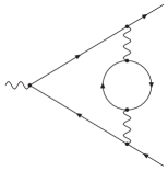
Figure 1: Fermionic vertex correction

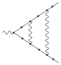
(a)

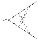
(b)

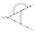
(c)

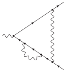
(d)

Figure 2: Abelian vertex corrections

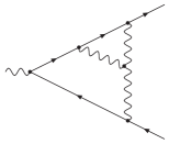
(a)

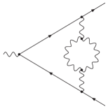
(b)

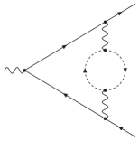
(c)

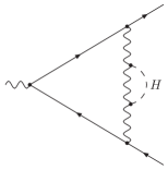
(d)

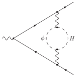
(e)

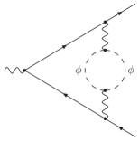
(f)

Figure 3: Non-Abelian vertex corrections

Solid lines with arrows denote fermions, wavy lines denote gauge bosons, short-dashed lines with arrows denote ghost fields and long-dashed lines stand for the Higgs boson ($H$) or Goldstone bosons ($\phi$), depending on the labels. The graphs in figures 2c), 2d) and 3a) also appear in a horizontally mirrored version, so their contributions have to be counted twice.

The three figures group the Feynman diagrams in subsets which are separately gauge-invariant when adding the corresponding renormalization contributions from section 4. The fermionic contribution of the graph in figure 1 is proportional to $n_{f}$, the number of fermions running in the closed fermion loop. Figure 2 represents the Abelian graphs (in addition to figure 1) which are present also in an unbroken $U(1)$ theory like QED. Finally figure 3 shows the non-Abelian graphs, which include the contributions from the Higgs mechanism. The Abelian contribution only counts the part of the graphs 2b) and 2c) which is proportional to $C_{F}^{2}$. The other part of these two graphs, which is proportional to $C_{F}C_{A}$, belongs to the non-Abelian contribution.

The fermionic contribution has been calculated exactly in Feucht:2003yx , i.e. for all $Q^{2}$, not only $Q^{2}\gg M^{2}$, showing the good agreement of the Sudakov limit with the exact contribution for energies larger than 300 GeV. The high-energy asymptotic limit of this result is quoted in section 3.2. Note that we state in this paper the individual vertex correction, self-energy correction and renormalization terms, whereas in Feucht:2003yx only the total fermionic contribution to the form factor is given.

The Abelian graphs have been evaluated in N⁴LL approximation, i.e. including all large logarithms and the non-logarithmic constant. These calculations are presented in sections 3.3 to 3.6. The non-Abelian graphs, especially figure 3a), are more complicated to evaluate, as they have three massive propagators each (compared to two for the Abelian graphs). We have only evaluated them in N³LL accuracy as the non-logarithmic constant is not needed for the insertion of the form factor result into the four-fermion amplitude. The corresponding calculations can be found in sections 3.7 and 3.8.

3.1 Reduction to scalar integrals

From each Feynman vertex diagram in the figures 1–3, by applying the Feynman rules in appendix A, we get a vertex amplitude of the following form:

$$\mathcal{F}_{\mathrm{v}}^{\mu}=\bar{\psi}(p_{1})\,\Gamma^{\mu}\,\psi(p_{2})\,,$$ (2)

where $\psi(p_{1,2})$ are doublets of Dirac spinors in the $SU(2)$ isospin space corresponding to the incoming and outgoing fermion, and $\Gamma^{\mu}$ is a quadratic matrix both in the spinor space and in the isospin space (for each Lorentz index $\mu$).

For vanishing fermion masses (in the Sudakov limit) the vertex amplitudes can be written as $\mathcal{F}_{\mathrm{v}}^{\mu}=F_{\mathrm{v}}\mathcal{F}_{\mathrm{B}}^{\mu}$, where $\mathcal{F}_{\mathrm{B}}^{\mu}$ is the Born amplitude and $F_{\mathrm{v}}$ is a contribution to the form factor. The scalar quantity $F_{\mathrm{v}}$ can be extracted from the vertex amplitude by projection (see e.g. Bernreuther:2004ih ):

$$F_{\mathrm{v}}=-\frac{\operatorname{Tr}(\gamma_{\mu}\makebox[0.0pt][l]{\hskip 3.24997pt\makebox[0.0pt]{/}}p_{1}\Gamma^{\mu}\makebox[0.0pt][l]{\hskip 3.24997pt\makebox[0.0pt]{/}}p_{2})}{4N(d-2)\,p_{1}\cdot p_{2}}\,,$$ (3)

where dimensional regularization 'tHooft:1972fi is used with $d=4-2\varepsilon$ as the number of space-time dimensions, and $N=2$ for $SU(2)$. The trace runs over the spinor and the isospin indices. By applying this projection, we get a linear combination of scalar loop integrals. For convenience, we separate the integration measure as follows:

$$\mu^{4-d}g^{2}\int\!\frac{\mathrm{d}^{d}k}{(2\pi)^{d}}=i\frac{\alpha}{4\pi}\left(\frac{\mu^{2}}{M^{2}}\right)^{\varepsilon}S_{\varepsilon}\left[e^{\varepsilon\gamma_{E}}(M^{2})^{\varepsilon}\int\!\frac{\mathrm{d}^{d}k}{i\pi^{d/2}}\right]$$ (4)

Here $\mu$ is the mass scale of dimensional regularization, $\alpha=g^{2}/(4\pi)$ with the weak coupling $g$, $\gamma_{E}$ is Euler’s constant and $S_{\varepsilon}=(4\pi)^{\varepsilon}e^{-\varepsilon\gamma_{E}}$. Within the $\overline{\text{MS}}$ renormalization scheme, $S_{\varepsilon}$ is absorbed into $\mu^{2\varepsilon}$ by a redefinition of $\mu$, and as we set $\mu=M$ in the end, the prefactor in front of the square brackets gets especially simple.

The reduction of the Feynman amplitudes to scalar integrals has been performed with the computer algebra program FORM Vermaseren:2000nd , and the evaluation of the scalar integrals, as described in the following sections, has been done with Mathematica Wolfram:Mathematica4.2 .

We have not performed a reduction of the scalar integrals to so-called master integrals by a method like integration by parts Tkachov:1981wb ; Chetyrkin:1981qh , as the number of scalar integrals obtained from the Feynman diagrams is not too big and most of the scalar integrals can easily be evaluated in a semi-automatical way starting from our expressions for general powers of the propagators, which are presented in the following sections.

3.2 Fermionic vertex correction

The fermionic vertex correction of figure 1 has been evaluated in Feucht:2003yx , where the integration of the inner fermion loop has been done first, leaving a one-loop integral feasible by the standard Feynman parametrization technique. The contribution of the fermionic vertex correction to the form factor is

$$F_{\mathrm{v},n_{f}} =C_{F}T_{F}n_{f}\left(\frac{\alpha}{4\pi}\right)^{2}\left(\frac{\mu^{2}}{M^{2}}\right)^{2\varepsilon}S_{\varepsilon}^{2}\,\Biggl{\{}$$

$$\qquad\frac{1}{\varepsilon}\left[\frac{4}{3}\mathcal{L}^{2}-\frac{20}{3}\mathcal{L}+\frac{8}{9}\pi^{2}+\frac{29}{3}\right]-\frac{8}{9}\mathcal{L}^{3}+\frac{56}{9}\mathcal{L}^{2}$$

$$\qquad+\left(\frac{4}{9}\pi^{2}-\frac{238}{9}\right)\mathcal{L}-\frac{8}{3}\zeta_{3}-\frac{38}{27}\pi^{2}+\frac{749}{18}\Biggr{\}}$$

$$\quad+\mathcal{O}(\varepsilon)+\mathcal{O}\!\left(\frac{M^{2}}{Q^{2}}\right),$$ (5)

where $\mathcal{L}=\ln(Q^{2}/M^{2})$, and $\zeta_{3}\approx 1.202057$ is a value of Riemann’s zeta function.

3.3 Planar vertex correction

The reduction (see section 3.1) of the planar Feynman graph in figure 2a) leads to scalar integrals corresponding to the graph in figure 4.

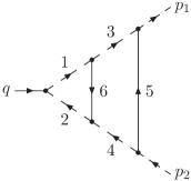
Figure 4: Scalar graph for planar vertex correction

The numbers enumerate the inner propagators and correspond to the indices $i$ of the propagator powers $n_{i}$ and of the inner momenta $k_{i}$, the directions of which are indicated by the arrows. Solid lines stand for massive propagators, dashed lines for massless ones.

Apart from propagators in the denominator, one scalar product remains in the numerator which cannot be expressed linearly in terms of the denominator. We have chosen this irreducible scalar product to be $2k_{5}\cdot(k_{5}-k_{6})$. The set of scalar integrals is then covered by the following function ($k=k_{5}$, $\ell=k_{5}-k_{6}$):

$$F_{\mathrm{LA}}(n_{1},\ldots,n_{7})=e^{2\varepsilon\gamma_{E}}\,(M^{2})^{2\varepsilon}\,(Q^{2})^{n-n_{7}-4}$$

$$\times\int\!\frac{\mathrm{d}^{d}k}{i\pi^{d/2}}\int\!\frac{\mathrm{d}^{d}\ell}{i\pi^{d/2}}\,\frac{(2k\cdot\ell)^{n_{7}}}{(\ell^{2}-2p_{1}\cdot\ell)^{n_{1}}\,(\ell^{2}-2p_{2}\cdot\ell)^{n_{2}}}$$

$$\times\frac{1}{(k^{2}-2p_{1}\cdot k)^{n_{3}}\,(k^{2}-2p_{2}\cdot k)^{n_{4}}\,(k^{2}-M^{2})^{n_{5}}}$$

$$\times\frac{1}{((k-\ell)^{2}-M^{2})^{n_{6}}}\,,$$ (6)

with $n=n_{123456}$, where we use $n_{ij\cdots}=n_{i}+n_{j}+\ldots$ as a shorthand notation. The scalar integrals have been defined in such a way that they do not carry a mass dimension.

The evaluation of the scalar integrals has been performed with the expansion by regions (see appendix B). The following regions contribute to the planar vertex correction Smirnov:2002pj :

(h-h): $$k\sim Q,\quad \ell\sim Q$$

(1c-h): $$k\;\|\;p_{1}, \ell\sim Q$$

(2c-h): $$k\;\|\;p_{2}, \ell\sim Q$$

(1c-1c): $$k\;\|\;p_{1}, \ell\;\|\;p_{1}$$

(2c-2c): $$k\;\|\;p_{2}, \ell\;\|\;p_{2}$$

(h-s’): $$k\sim Q, k_{6}=k-\ell\sim M$$

By $k\sim Q$ we mean that each component of the vector $k$ is of the order of $Q$. And $k\;\|\;p_{i}$ indicates a region where the momentum $k$ is collinear to the external momentum $p_{i}$:

$$k\;\|\;p_{1} \iff k_{+}\sim\frac{M^{2}}{Q}\,,\quad k_{-}\sim Q\,,\quad k_{\bot}\sim M\,,$$ (7)

$$k\;\|\;p_{2} \iff k_{+}\sim Q\,,\quad k_{-}\sim\frac{M^{2}}{Q}\,,\quad k_{\bot}\sim M\,,$$ (8)

where $k_{\pm}=(2p_{1,2}\cdot k)/Q$ denotes the components of $k$ in the direction of $p_{2}$ and $p_{1}$ respectively, and the vector $k_{\bot}=k-(k_{-}/Q)p_{1}-(k_{+}/Q)p_{2}$ is made up of the components of $k$ perpendicular to $p_{1,2}$.

The leading term in the expansion of the (h-h) region corresponds to the massless integral with $M=0$, which is well known Kramer:1986sg ; Kramer:1986sgE ; Matsuura:1988sm . The (h-s’) region is of order $(M^{2}/Q^{2})^{2-n_{6}+\varepsilon}$ and therefore suppressed by at least one factor $M^{2}/Q^{2}$ with respect to the (h-h) region for all scalar integrals we need, i.e. for $n_{i}\leq 1$, $i=1,\ldots,6$. So we do not need to consider the (h-s’) region. The (1c-1c) region is of order $(M^{2}/Q^{2})^{4-n_{1356}+n_{7}}$, the (2c-2c) region of order $(M^{2}/Q^{2})^{4-n_{2456}+n_{7}}$. Both are suppressed if $n_{7}>0$, i.e. if the numerator is present, and are only evaluated for $n_{7}=0$. The leading contributions from the (1c-h) and (1c-1c) regions can be expressed by one- and two-fold Mellin–Barnes representations (see appendix C):

$$F_{\mathrm{LA}}^{\text{(1c-h)}}(n_{1},\ldots,n_{7})=\left(\frac{M^{2}}{Q^{2}}\right)^{2-n_{35}+\varepsilon}\,e^{-ni\pi}\,e^{2\varepsilon\gamma_{E}}$$

$$\times\frac{\Gamma(\frac{d}{2}-n_{3})\Gamma(\frac{d}{2}-n_{16}+n_{7})\Gamma(n_{35}-\frac{d}{2})}{\Gamma(n_{1})\Gamma(n_{2})\Gamma(n_{3})\Gamma(n_{5})\Gamma(n_{6})\Gamma(d-n_{126}+n_{7})}$$

$$\times\int_{-i\infty}^{i\infty}\!\frac{\mathrm{d}z}{2\pi i}\,\Gamma(-z)\Gamma(\tfrac{d}{2}-n_{26}-z)$$

$$\times\frac{\Gamma(n_{6}+z)\Gamma(n_{37}-n_{4}+z)\Gamma(n_{126}-\frac{d}{2}+z)}{\Gamma(\frac{d}{2}-n_{4}+n_{7}+z)}\,,$$ (9)

$$F_{\mathrm{LA}}^{\text{(1c-1c)}}(n_{1},\ldots,n_{6},n_{7}=0)=\left(\frac{M^{2}}{Q^{2}}\right)^{4-n_{1356}}\,e^{-ni\pi}\,e^{2\varepsilon\gamma_{E}}$$

$$\times\frac{1}{\Gamma(n_{1})\Gamma(n_{3})\Gamma(n_{5})\Gamma(n_{6})\Gamma(\frac{d}{2}-n_{24})}\int_{-i\infty}^{i\infty}\!\frac{\mathrm{d}z_{1}}{2\pi i}\int_{-i\infty}^{i\infty}\!\frac{\mathrm{d}z_{2}}{2\pi i}$$

$$\times\frac{\Gamma(-z_{1})\Gamma(n_{13}-\frac{d}{2}-z_{1})\Gamma(\frac{d}{2}-n_{1}+z_{1})}{\Gamma(\frac{d}{2}-n_{4}+z_{1})}$$

$$\times\Gamma(\tfrac{d}{2}-n_{24}+z_{1})\,\frac{\Gamma(-z_{2})\Gamma(\frac{d}{2}-n_{35}-z_{2})}{\Gamma(\frac{d}{2}-n_{5}-z_{2})}$$

$$\times\Gamma(\tfrac{d}{2}-n_{45}-z_{2})\Gamma(n_{1356}-d+z_{2})\Gamma(n_{5}+z_{1}+z_{2})\,.$$ (10)

For symmetry reasons we get $F_{\mathrm{LA}}^{\text{(2c-h)}}$ from $F_{\mathrm{LA}}^{\text{(1c-h)}}$ and $F_{\mathrm{LA}}^{\text{(2c-2c)}}$ from $F_{\mathrm{LA}}^{\text{(1c-1c)}}$ by exchanging $n_{1}\leftrightarrow n_{2}$ and $n_{3}\leftrightarrow n_{4}$.

The integration contour of the Mellin–Barnes integrals runs from $-i\infty$ to $+i\infty$ in such a way that poles from gamma functions of the form $\Gamma(\ldots+z)$ lie on the left hand side of the contour (“left poles”) and poles from gamma functions of the form $\Gamma(\ldots-z)$ lie on the right hand side of the contour (“right poles”).

The Mellin–Barnes integrals in (3.3) and (3.3) are solved by closing the integration contours either at positive or negative real infinity and summing over the residues within the contour. The integrals develop singularities at points in the parameter space of the $n_{i}$ where a left pole and a right pole glue together in one point. Some of these singularities are cancelled by zeros originating from gamma functions in the denominator, e.g. in $F_{\mathrm{LA}}^{\text{(1c-h)}}$ when $n_{6}=0$. Here the result is given by the limit $n_{6}\to 0$ to which only the residue of the integrand at $z=0$ or $z=-n_{6}$ contributes.

Other singularities in the parameter space are cancelled between several regions. This is the case for the pole $1/(n_{3}-n_{4})$ which is cancelled between the (1c-h) and the (2c-h) regions. Another pole $1/(n_{13}-n_{24})$ is cancelled between the (1c-1c) and the (2c-2c) regions. Such singularities, which are regularized analytically with the parameters $n_{i}$ in individual regions, are typical for collinear regions in the Sudakov limit. The sum of the contributions from all regions is well-defined in the framework of dimensional regularization.

In some cases, the first Barnes lemma (see appendix C) is used to solve one of the two Mellin–Barnes integrations in (3.3). In more complicated cases first all residues which produce singularities are extracted, and the limits of the analytic regularization and of dimensional regularization ($\varepsilon\to 0$) are performed before summing up the remaining residues. These sums are then solved by Mathematica or looked up in a summation table (e.g. in Smirnov:2004ym ).

By adding together the contributions from all regions we have obtained the results for all scalar integrals originating from the reduction of the planar Feynman diagram. As examples, we show the results for the scalar graph with all propagators present and various powers of the numerator:

$$\!\!F_{\mathrm{LA}}(1,1,1,1,1,1,0)=\frac{1}{24}\mathcal{L}^{4}+\frac{\pi^{2}}{3}\mathcal{L}^{2}-6\zeta_{3}\mathcal{L}+\frac{31}{180}\pi^{4}\,,$$ (11)

$$\!\!F_{\mathrm{LA}}(1,1,1,1,1,1,1)=\frac{\pi^{2}}{3}\mathcal{L}-10\zeta_{3}\,,$$ (12)

$$\!\!F_{\mathrm{LA}}(1,1,1,1,1,1,2)=\frac{1}{2\varepsilon^{2}}+\frac{1}{\varepsilon}\left(-\mathcal{L}+\frac{7}{2}\right)$$

$$+\mathcal{L}^{2}+\left(\frac{\pi^{2}}{6}-8\right)\mathcal{L}-11\zeta_{3}+\frac{\pi^{2}}{12}+\frac{37}{2}\,.$$ (13)

Here and for all other results of individual scalar integrals, we omit the specification “${}+\mathcal{O}(\varepsilon)+\mathcal{O}(M^{2}/Q^{2})$” of the neglected terms. The result (11) has already been calculated in Smirnov:1997gx .

The complete Feynman diagram in figure 2a) involving contributions from all scalar integrals with different $n_{i}$ yields the following planar vertex correction:

$$F_{\mathrm{v},\mathrm{LA}} =C_{F}^{2}\left(\frac{\alpha}{4\pi}\right)^{2}\left(\frac{\mu^{2}}{M^{2}}\right)^{2\varepsilon}S_{\varepsilon}^{2}\,\Biggl{\{}\frac{1}{2\varepsilon^{2}}$$

$$\qquad+\frac{1}{\varepsilon}\left[-\mathcal{L}^{2}+3\mathcal{L}-\frac{2}{3}\pi^{2}-\frac{11}{4}\right]+\frac{1}{6}\mathcal{L}^{4}$$

$$\qquad+\left(\frac{2}{3}\pi^{2}-1\right)\mathcal{L}^{2}+\left(-32\zeta_{3}-\pi^{2}+\frac{11}{2}\right)\mathcal{L}$$

$$\qquad+\frac{8}{15}\pi^{4}+62\zeta_{3}+\frac{13}{12}\pi^{2}-\frac{41}{8}\Biggr{\}}$$

$$\quad+\mathcal{O}(\varepsilon)+\mathcal{O}\!\left(\frac{M^{2}}{Q^{2}}\right).$$ (14)

3.4 Non-planar vertex correction

The non-planar Feynman graph in figure 2b) involves the scalar integrals depicted in figure 5. With the choice $2k_{5}\cdot k_{6}$ for the irreducible scalar product, the scalar integrals are written as

$$F_{\mathrm{NP}}(n_{1},\ldots,n_{7})=e^{2\varepsilon\gamma_{E}}\,(M^{2})^{2\varepsilon}\,(Q^{2})^{n-n_{7}-4}$$

$$\times\int\!\frac{\mathrm{d}^{d}k}{i\pi^{d/2}}\int\!\frac{\mathrm{d}^{d}\ell}{i\pi^{d/2}}\,\frac{(2k\cdot\ell)^{n_{7}}}{((p_{1}-k-\ell)^{2})^{n_{1}}\,((p_{2}-k-\ell)^{2})^{n_{2}}}$$

$$\times\frac{1}{(k^{2}-2p_{1}\cdot k)^{n_{3}}\,(\ell^{2}-2p_{2}\cdot\ell)^{n_{4}}\,(k^{2}-M^{2})^{n_{5}}}$$

$$\times\frac{1}{(\ell^{2}-M^{2})^{n_{6}}}\,,$$ (15)

with $k=k_{5}$ and $\ell=k_{6}$.

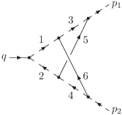
Figure 5: Scalar graph for non-planar vertex correction

The following regions contribute to the non-planar vertex correction Smirnov:1998vk ; Smirnov:2002pj :

(h-h): $$k\sim Q,\quad \ell\sim Q$$

(1c-h): $$k\;\|\;p_{1}, \ell\sim Q$$

(h-2c): $$k\sim Q, \ell\;\|\;p_{2}$$

(1c-1c): $$k\;\|\;p_{1}, \ell\;\|\;p_{1}$$

(2c-2c): $$k\;\|\;p_{2}, \ell\;\|\;p_{2}$$

(1c-2c): $$k\;\|\;p_{1}, \ell\;\|\;p_{2}$$

(1c-1c’): $$k\;\|\;p_{1}, k_{4}\;\|\;p_{1}$$

(2c’-2c): $$k_{3}\;\|\;p_{2}, \ell\;\|\;p_{2}$$

(us’-us’): $$k_{3}\sim M^{2}/Q,\quad k_{4}\sim M^{2}/Q$$

(1c-us’): $$k\;\|\;p_{1}, k_{4}\sim M^{2}/Q$$

(us’-2c): $$k_{3}\sim M^{2}/Q, \ell\;\|\;p_{2}$$

The leading term of the (h-h) region is known from the massless case Kramer:1986sg ; Kramer:1986sgE ; Matsuura:1988sm . As for the planar vertex correction in the previous section, the (1c-1c) and the (2c-2c) regions are of order $(M^{2}/Q^{2})^{4-n_{1356}+n_{7}}$ and $(M^{2}/Q^{2})^{4-n_{2456}+n_{7}}$ respectively. They are suppressed for $n_{7}>0$ and are therefore evaluated only for $n_{7}=0$. The leading contributions from the regions, apart from (h-h), can be written as one-fold Mellin–Barnes integrals or simpler expressions:

$$F_{\mathrm{NP}}^{\text{(1c-h)}}(n_{1},\ldots,n_{7})=\left(\frac{M^{2}}{Q^{2}}\right)^{2-n_{35}+\varepsilon}\,e^{-ni\pi}\,e^{2\varepsilon\gamma_{E}}$$

$$\times\frac{\Gamma(\frac{d}{2}-n_{24})\Gamma(\frac{d}{2}-n_{16}+n_{7})\Gamma(n_{35}-\frac{d}{2})}{\Gamma(n_{1})\Gamma(n_{2})\Gamma(n_{3})\Gamma(n_{5})\,\Gamma(d-n_{1246}+n_{7})^{2}}\int_{-i\infty}^{i\infty}\!\frac{\mathrm{d}z}{2\pi i}$$

$$\times\frac{\Gamma(-z)\Gamma(\frac{d}{2}-n_{146}-z)\Gamma(\frac{d}{2}-n_{1246}+n_{37}-z)}{\Gamma(\frac{d}{2}-n_{16}-z)}$$

$$\times\frac{\Gamma(n_{1}+z)\Gamma(\frac{d}{2}-n_{3}+z)\Gamma(n_{1246}-\frac{d}{2}+z)}{\Gamma(n_{16}+z)}\,,$$ (16)

$$F_{\mathrm{NP}}^{\text{(1c-1c)}}(n_{1},\ldots,n_{6},n_{7}=0)=\left(\frac{M^{2}}{Q^{2}}\right)^{4-n_{1356}}e^{-ni\pi}\,e^{2\varepsilon\gamma_{E}}$$

$$\times\frac{\Gamma(n_{16}-\frac{d}{2})\Gamma(n_{1356}-d)}{\Gamma(n_{1})\Gamma(n_{3})\Gamma(n_{5})\Gamma(n_{6})\Gamma(\frac{d}{2}-n_{24})}\int_{-i\infty}^{i\infty}\!\frac{\mathrm{d}z}{2\pi i}\,\Gamma(-z)$$

$$\times\Gamma(n_{13}-\tfrac{d}{2}-z)\,\frac{\Gamma(n_{5}-n_{4}+z)\Gamma(\frac{d}{2}-n_{1}+z)}{\Gamma(n_{156}-n_{4}-\frac{d}{2}+z)}$$

$$\times\frac{\Gamma(\frac{d}{2}-n_{24}+z)\Gamma(\frac{d}{2}-n_{34}+z)}{\Gamma(\frac{d}{2}-n_{4}+z)}\,,$$ (17)

$$F_{\mathrm{NP}}^{\text{(1c-2c)}}(n_{1},\ldots,n_{7})=\left(\frac{M^{2}}{Q^{2}}\right)^{4-n_{3456}}e^{-ni\pi}\,e^{2\varepsilon\gamma_{E}}$$

$$\times\frac{\Gamma(n_{37}-n_{2})\Gamma(n_{47}-n_{1})\Gamma(\frac{d}{2}-n_{13})\Gamma(\frac{d}{2}-n_{24})}{\Gamma(n_{3})\Gamma(n_{4})\Gamma(n_{5})\Gamma(n_{6})\,\Gamma(\frac{d}{2}-n_{12}+n_{7})^{2}}$$

$$\times\Gamma(n_{35}-\tfrac{d}{2})\Gamma(n_{46}-\tfrac{d}{2})\,,$$ (18)

$$F_{\mathrm{NP}}^{\text{(1c-1c')}}(n_{1},\ldots,n_{7})=\left(\frac{M^{2}}{Q^{2}}\right)^{4-n_{2345}}e^{-ni\pi}\,e^{2\varepsilon\gamma_{E}}$$

$$\times\frac{\Gamma(d-n_{234})\Gamma(n_{24}-\frac{d}{2})\Gamma(n_{2345}-d)}{\Gamma(n_{2})\Gamma(n_{3})\Gamma(n_{4})\Gamma(n_{5})\Gamma(\frac{d}{2}-n_{16}+n_{7})\Gamma(d-n_{2347})}$$

$$\times\int_{-i\infty}^{i\infty}\!\frac{\mathrm{d}z}{2\pi i}\,\Gamma(-z)\Gamma(\tfrac{d}{2}-n_{347}-z)\Gamma(n_{37}-n_{6}+z)$$

$$\times\frac{\Gamma(\frac{d}{2}-n_{2}+z)\Gamma(\frac{d}{2}-n_{16}+n_{7}+z)}{\Gamma(\frac{d}{2}-n_{6}+n_{7}+z)}\,,$$ (19)

$$F_{\mathrm{NP}}^{\text{(us'-us')}}(n_{1},\ldots,n_{7})=\left(\frac{M^{2}}{Q^{2}}\right)^{8-n_{1256}-2n_{34}-2\varepsilon}\,e^{-ni\pi}$$

$$\times e^{2\varepsilon\gamma_{E}}\,\frac{\Gamma(d-n_{134})\Gamma(d-n_{234})\Gamma(n_{13}-\tfrac{d}{2})\Gamma(n_{24}-\tfrac{d}{2})}{\Gamma(n_{1})\Gamma(n_{2})\Gamma(n_{3})\Gamma(n_{4})\Gamma(n_{5})\Gamma(n_{6})}$$

$$\times\Gamma(n_{2345}-d)\Gamma(n_{1346}-d)\,,$$ (20)

$$F_{\mathrm{NP}}^{\text{(1c-us')}}(n_{1},\ldots,n_{7})=\left(\frac{M^{2}}{Q^{2}}\right)^{6-n_{2356}-2n_{4}-\varepsilon}\,e^{-ni\pi}\,e^{2\varepsilon\gamma_{E}}$$

$$\times\frac{\Gamma(\tfrac{d}{2}-n_{4})\Gamma(\tfrac{d}{2}-n_{13})\Gamma(d-n_{234})\Gamma(n_{24}-\frac{d}{2})}{\Gamma(n_{2})\Gamma(n_{3})\Gamma(n_{4})\Gamma(n_{5})\Gamma(n_{6})\Gamma(n_{47}-n_{1})\Gamma(\frac{d}{2}-n_{3})}$$

$$\times\Gamma(n_{46}-\tfrac{d}{2})\Gamma(n_{347}-\tfrac{d}{2})\Gamma(n_{2345}-d)\,.$$ (21)

Using the symmetry of the non-planar graph under the exchange of the parameters $n_{1}\leftrightarrow n_{2}$, $n_{3}\leftrightarrow n_{4}$ and $n_{5}\leftrightarrow n_{6}$, one gets $F_{\mathrm{NP}}^{\text{(h-2c)}}$ from $F_{\mathrm{NP}}^{\text{(1c-h)}}$, $F_{\mathrm{NP}}^{\text{(2c-2c)}}$ from $F_{\mathrm{NP}}^{\text{(1c-1c)}}$, $F_{\mathrm{NP}}^{\text{(2c'-2c)}}$ from $F_{\mathrm{NP}}^{\text{(1c-1c')}}$ and $F_{\mathrm{NP}}^{\text{(us'-2c)}}$ from $F_{\mathrm{NP}}^{\text{(1c-us')}}$. The expression (3.4) for the (us’-us’) region is valid for general $n_{7}$ although it does not involve $n_{7}$ explicitly: The only dependence on $n_{7}$ of this region is cancelled by the prefactor $(Q^{2})^{-n_{7}}$ in (3.4).

We have checked the completeness of our set of regions by writing the full scalar integral for arbitrary parameters $n_{i}$ (except $n_{7}=0$) as a four-fold Mellin–Barnes representation. From this expression, we have extracted the residues yielding the non-suppressed contributions and have found 11 terms with exactly the same dependence on $M^{2}/Q^{2}$ as the 11 regions listed above.

The evaluation of the Mellin–Barnes integrals is done as described in the previous section. The structure of singularities needing analytic regularization is more complicated than in the planar case. Various poles involving combinations of the parameters $n_{i}$ are cancelled between the collinear regions (1c-1c), (2c-2c), (1c-2c), (1c-1c’) and (2c’-2c).

The contributions of all regions sum up to the results for the scalar integrals originating from the reduction of the non-planar Feynman diagram. Examples of these results are

$$\!\!F_{\mathrm{NP}}(1,1,1,1,1,1,0)=\frac{7}{12}\mathcal{L}^{4}-\frac{\pi^{2}}{6}\mathcal{L}^{2}+20\zeta_{3}\mathcal{L}-\frac{31}{180}\pi^{4}\,,$$ (22)

$$\!\!F_{\mathrm{NP}}(1,1,1,1,1,1,1)=\frac{1}{4}\mathcal{L}^{4}-\frac{\pi^{2}}{6}\mathcal{L}^{2}+14\zeta_{3}\mathcal{L}-\frac{\pi^{4}}{90}\,,$$ (23)

$$\!\!F_{\mathrm{NP}}(1,1,1,1,1,1,2)=\frac{2}{\varepsilon^{2}}+\frac{1}{\varepsilon}(-4\mathcal{L}+7)+\frac{1}{4}\mathcal{L}^{4}-\mathcal{L}^{3}$$

$$+\left(-\frac{\pi^{2}}{6}+9\right)\mathcal{L}^{2}+(14\zeta_{3}-30)\mathcal{L}-\frac{\pi^{4}}{90}-4\zeta_{3}+\frac{\pi^{2}}{3}$$

$$+38\,,$$ (24)

$$\!\!F_{\mathrm{NP}}(1,1,1,1,1,1,3)=\frac{7}{2\varepsilon^{2}}+\frac{1}{\varepsilon}\left(-7\mathcal{L}+\frac{111}{8}\right)$$

$$+\frac{1}{4}\mathcal{L}^{4}-\frac{3}{2}\mathcal{L}^{3}+\left(-\frac{\pi^{2}}{6}+\frac{59}{4}\right)\mathcal{L}^{2}+\left(14\zeta_{3}-\frac{211}{4}\right)\mathcal{L}$$

$$-\frac{\pi^{4}}{90}-6\zeta_{3}+\frac{3}{4}\pi^{2}+\frac{571}{8}\,.$$ (25)

The result (22) for the scalar graph without numerator is known from Smirnov:1998vk . The complete non-planar vertex correction with contributions from all scalar integrals is as follows:

$$F_{\mathrm{v},\mathrm{NP}} =\left(C_{F}^{2}-\frac{1}{2}C_{F}C_{A}\right)\left(\frac{\alpha}{4\pi}\right)^{2}\left(\frac{\mu^{2}}{M^{2}}\right)^{2\varepsilon}S_{\varepsilon}^{2}\,\Biggl{\{}-\frac{2}{\varepsilon}$$

$$\qquad+\frac{1}{3}\mathcal{L}^{4}-\frac{8}{3}\mathcal{L}^{3}+\left(-\frac{2}{3}\pi^{2}+12\right)\mathcal{L}^{2}$$

$$\qquad+\left(40\zeta_{3}+\frac{2}{3}\pi^{2}-28\right)\mathcal{L}-\frac{4}{15}\pi^{4}-72\zeta_{3}-\pi^{2}$$

$$\qquad+28\Biggr{\}}+\mathcal{O}(\varepsilon)+\mathcal{O}\!\left(\frac{M^{2}}{Q^{2}}\right)\,.$$ (26)

3.5 Vertex correction with Mercedes–Benz graph

Figure 6 illustrates the scalar integrals resulting from the reduction of the Mercedes–Benz graph in figure 2c).

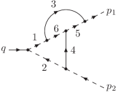
Figure 6: Scalar Mercedes–Benz graph

With our choice of $2p_{2}\cdot k_{5}$ as the irreducible scalar product, the scalar integrals are defined as

$$F_{\mathrm{BE}}(n_{1},\ldots,n_{7})=e^{2\varepsilon\gamma_{E}}\,(M^{2})^{2\varepsilon}\,(Q^{2})^{n-n_{7}-4}$$

$$\times\int\!\frac{\mathrm{d}^{d}k}{i\pi^{d/2}}\int\!\frac{\mathrm{d}^{d}\ell}{i\pi^{d/2}}\,\frac{(2p_{2}\cdot k)^{n_{7}}}{(\ell^{2}-2p_{1}\cdot\ell)^{n_{1}}\,(\ell^{2}-2p_{2}\cdot\ell)^{n_{2}}}$$

$$\times\frac{1}{(k^{2}-2p_{1}\cdot k-M^{2})^{n_{3}}\,(\ell^{2}-M^{2})^{n_{4}}\,(k^{2})^{n_{5}}\,((k-\ell)^{2})^{n_{6}}}\,,$$ (27)

with $k=k_{5}$ and $\ell=k_{4}$. The list of relevant regions for the Mercedes–Benz graph is shown here:

(h-h): $$k\sim Q,\quad \ell\sim Q$$

(1c-h): $$k\;\|\;p_{1}, \ell\sim Q$$

(h-2c): $$k\sim Q, \ell\;\|\;p_{2}$$

(us-2c): $$k\sim M^{2}/Q,\quad \ell\;\|\;p_{2}$$

(1c-1c): $$k\;\|\;p_{1}, \ell\;\|\;p_{1}$$

(2c-2c): $$k\;\|\;p_{2}, \ell\;\|\;p_{2}$$

(1c-2c): $$k\;\|\;p_{1}, \ell\;\|\;p_{2}$$

The leading contributions of all regions could be evaluated for general $n_{7}$, but the (us-2c) and the (2c-2c) region are only non-suppressed for $n_{7}=0$:

$$F_{\mathrm{BE}}^{\text{(h-h)}}(n_{1},\ldots,n_{7})=\left(\frac{M^{2}}{Q^{2}}\right)^{2\varepsilon}e^{-ni\pi}\,e^{2\varepsilon\gamma_{E}}\sum_{i_{1},i_{2},i_{3}\geq 0}^{i_{123}\leq n_{7}}$$

$$\times\frac{n_{7}!}{i_{1}!\,i_{2}!\,i_{3}!\,(n_{7}-i_{123})!}\,\frac{\Gamma(n_{1}+i_{3})\Gamma(n_{4}+i_{2})}{\Gamma(n_{1})\Gamma(n_{2})\Gamma(n_{3})\Gamma(n_{4})}$$

$$\times\frac{\Gamma(\frac{d}{2}-n_{35})\Gamma(d-n_{13456}+i_{1})\Gamma(n_{123456}-d)}{\Gamma(n_{5})\Gamma(n_{6})\Gamma(d-n_{356}+i_{123})\Gamma(\frac{3}{2}d-n_{123456}+n_{7})}$$

$$\times\int_{-i\infty}^{i\infty}\!\frac{\mathrm{d}z}{2\pi i}\,\Gamma(-z)\Gamma(\tfrac{d}{2}-n_{56}+i_{12}-z)\Gamma(n_{5}+z)$$

$$\times\Gamma(\tfrac{d}{2}-n_{24}+n_{7}-i_{12}+z)\,\frac{\Gamma(n_{3567}-i_{123}-\frac{d}{2}+z)}{\Gamma(n_{13567}-i_{12}-\frac{d}{2}+z)}$$

$$\times\frac{\Gamma(d-n_{36}-2n_{5}+i_{123}-z)}{\Gamma(d-n_{36}-2n_{5}+i_{12}-z)}\,,$$ (28)

$$F_{\mathrm{BE}}^{\text{(1c-h)}}(n_{1},\ldots,n_{7})=\left(\frac{M^{2}}{Q^{2}}\right)^{2-n_{35}+\varepsilon}\,e^{-ni\pi}\,e^{2\varepsilon\gamma_{E}}$$

$$\times\frac{\Gamma(n_{35}-\frac{d}{2})\Gamma(\frac{d}{2}-n_{146})}{\Gamma(n_{1})\Gamma(n_{2})\Gamma(n_{3})\Gamma(n_{6})\Gamma(d-n_{1246})}$$

$$\times\int_{-i\infty}^{i\infty}\!\frac{\mathrm{d}z}{2\pi i}\,\Gamma(-z)\Gamma(\tfrac{d}{2}-n_{246}-z)$$

$$\times\frac{\Gamma(n_{6}+z)\Gamma(\frac{d}{2}-n_{5}+n_{7}+z)\Gamma(n_{1246}-\frac{d}{2}+z)}{\Gamma(\frac{d}{2}+n_{7}+z)}\,,$$ (29)

$$F_{\mathrm{BE}}^{\text{(h-2c)}}(n_{1},\ldots,n_{7})=\left(\frac{M^{2}}{Q^{2}}\right)^{2-n_{24}+\varepsilon}\,e^{-ni\pi}\,e^{2\varepsilon\gamma_{E}}$$

$$\times\frac{\Gamma(\frac{d}{2}-n_{2})\Gamma(\frac{d}{2}-n_{35})\Gamma(\frac{d}{2}-n_{1356}+n_{2})}{\Gamma(n_{2})\Gamma(n_{3})\Gamma(n_{4})\Gamma(n_{6})}$$

$$\times\frac{\Gamma(\frac{d}{2}-n_{56}+n_{7})\Gamma(n_{24}-\frac{d}{2})\Gamma(n_{356}-\frac{d}{2})}{\Gamma(d-n_{1356})\Gamma(d-n_{356}+n_{7})}\,,$$ (30)

$$F_{\mathrm{BE}}^{\text{(us-2c)}}(n_{1},\ldots,n_{7})=\left(\frac{M^{2}}{Q^{2}}\right)^{6-n_{2346}-2n_{5}+n_{7}-\varepsilon}e^{-ni\pi}$$

$$\times e^{2\varepsilon\gamma_{E}}\,\frac{\Gamma(\frac{d}{2}-n_{5}+n_{7})\Gamma(d-n_{256}+n_{7})\Gamma(n_{35}-\tfrac{d}{2})}{\Gamma(n_{2})\Gamma(n_{3})\Gamma(n_{4})\Gamma(n_{5})\Gamma(n_{6})\Gamma(n_{5}-n_{17})}$$

$$\times\Gamma(n_{25}-n_{17}-\tfrac{d}{2})\Gamma(n_{56}-n_{7}-\tfrac{d}{2})\Gamma(n_{2456}-n_{7}-d)\,,$$ (31)

$$F_{\mathrm{BE}}^{\text{(1c-1c)}}(n_{1},\ldots,n_{7})=\left(\frac{M^{2}}{Q^{2}}\right)^{4-n_{13456}}e^{-ni\pi}\,e^{2\varepsilon\gamma_{E}}$$

$$\times\sum_{i_{1},i_{2}\geq 0}^{i_{12}\leq n_{7}}\,\frac{n_{7}!}{i_{1}!\,i_{2}!\,(n_{7}-i_{12})!}\,\frac{\Gamma(n_{1}+i_{2})}{\Gamma(n_{1})\Gamma(n_{3})\Gamma(n_{4})\Gamma(n_{5})}$$

$$\times\frac{1}{\Gamma(n_{6})\Gamma(\frac{d}{2}-n_{2}+n_{7})}\int_{-i\infty}^{i\infty}\!\frac{\mathrm{d}z_{1}}{2\pi i}\int_{-i\infty}^{i\infty}\!\frac{\mathrm{d}z_{2}}{2\pi i}\,\Gamma(-z_{1})$$

$$\times\frac{\Gamma(n_{16}-i_{1}-\frac{d}{2}-z_{1})\Gamma(n_{1356}-i_{1}-d-z_{1})}{\Gamma(n_{1}+i_{2}-z_{1})}$$

$$\times\Gamma(n_{4}+i_{1}+z_{1})\Gamma(-z_{2})\Gamma(\tfrac{d}{2}-n_{56}+i_{1}-z_{2})$$

$$\times\Gamma(n_{5}+z_{2})\,\frac{\Gamma(n_{1}-n_{5}+i_{2}-z_{1}-z_{2})}{\Gamma(n_{1}-n_{5}-z_{1}-z_{2})}$$

$$\times\Gamma(\tfrac{d}{2}-n_{1}+n_{7}-i_{2}+z_{1}+z_{2})$$

$$\times\frac{\Gamma(\frac{d}{2}-n_{2}+n_{7}+z_{1}+z_{2})}{\Gamma(\frac{d}{2}+n_{7}+z_{1}+z_{2})}\,,$$ (32)

$$F_{\mathrm{BE}}^{\text{(2c-2c)}}(n_{1},\ldots,n_{7})=\left(\frac{M^{2}}{Q^{2}}\right)^{4-n_{2456}+n_{7}}\,e^{-ni\pi}\,e^{2\varepsilon\gamma_{E}}$$

$$\times\sum_{i_{1},i_{2},i_{3}\geq 0}^{i_{123}\leq n_{7}}\frac{n_{7}!}{i_{1}!\,i_{2}!\,i_{3}!\,(n_{7}-i_{123})!}\,\frac{\Gamma(n_{1}+i_{1})\Gamma(n_{37}-i_{1})}{\Gamma(n_{1})\Gamma(n_{2})\Gamma(n_{3})}$$

$$\times\frac{\Gamma(n_{2}-n_{137}+i_{2})}{\Gamma(n_{4})\Gamma(n_{5})\Gamma(n_{6})}\,\frac{\Gamma(\tfrac{d}{2}-n_{35}+i_{1})\Gamma(\frac{d}{2}-n_{6}+i_{23})}{\Gamma(\frac{d}{2}-n_{13})\Gamma(d-n_{356}+i_{123})}$$

$$\times\Gamma(d-n_{256}+n_{7}+i_{3})\Gamma(n_{56}-i_{23}-\tfrac{d}{2})$$

$$\times\Gamma(n_{2456}-n_{7}-d)\,,$$ (33)

$$F_{\mathrm{BE}}^{\text{(1c-2c)}}(n_{1},\ldots,n_{7})=\left(\frac{M^{2}}{Q^{2}}\right)^{4-n_{2345}}\,e^{-ni\pi}\,e^{2\varepsilon\gamma_{E}}$$

$$\times\frac{\Gamma(n_{2}-n_{16})\Gamma(\frac{d}{2}-n_{2})\Gamma(\frac{d}{2}-n_{56}+n_{7})\Gamma(n_{24}-\frac{d}{2})}{\Gamma(n_{2})\Gamma(n_{3})\Gamma(n_{4})\Gamma(\frac{d}{2}-n_{16})\Gamma(\frac{d}{2}-n_{6}+n_{7})}$$

$$\times\Gamma(n_{35}-\tfrac{d}{2})\,.$$ (34)

For the summation indices we use the shorthand notation $i_{12\cdots}=i_{1}+i_{2}+\ldots$, and the multiple summation is defined in the following way:

$$\sum_{i_{1},i_{2},\ldots\geq 0}^{i_{12\cdots}\leq n_{7}}=\sum_{i_{1}=0}^{n_{7}}\sum_{i_{2}=0}^{n_{7}-i_{1}}\cdots$$

We were able to reproduce the above expressions (3.5)–(3.5) for the regions by writing the full scalar integral with general $n_{i}$ as a triple sum over a three-fold Mellin–Barnes integral and extracting all non-suppressed contributions. Our evaluation of the (h-h) region is in agreement with the known results for the massless diagram Kramer:1986sg ; Kramer:1986sgE ; Matsuura:1988sm .

The (1c-1c) region is of order $(M^{2}/Q^{2})^{-1}$ when $n_{1}=n_{3}=n_{4}=n_{5}=n_{6}=1$. But in all these cases the inverse power of $M^{2}$ is cancelled by a factor of $M^{2}$ in the coefficient originating from the reduction to scalar integrals. The purely collinear regions (1c-1c), (2c-2c) and (1c-2c) develop poles at several points in the parameter space of the $n_{i}$ which need to be regularized analytically and cancel between these three regions.

The most complicated evaluation of the contributions to the Mercedes–Benz graph has to be performed for the (1c-1c) region with its two-fold Mellin–Barnes integral, especially when all propagators are present, $n_{1}=\cdots=n_{6}=1$, for $n_{7}=0,1,2$. In these three cases $F_{\mathrm{BE}}$ is of order $(M^{2}/Q^{2})^{-1}$, as described in the previous paragraph, and only the (1c-1c) region contributes to the leading term. In addition, the integrals are finite with respect to both dimensional and analytic regularization, and they result in simply a numerical constant times $(Q^{2}/M^{2})$. To evaluate these three complicated integrals, where none of the two integrations can be performed explicitly due to Barnes lemmas (see appendix C), we used the following strategy exemplified here by $F_{\mathrm{BE}}(1,1,1,1,1,1,0)$. After setting $d=4$ ($\varepsilon=0$) and applying some simplifications, equation (3.5) yields

$$F_{\mathrm{BE}}(1,1,1,1,1,1,0)=-\frac{Q^{2}}{M^{2}}\int_{-i\infty}^{i\infty}\!\frac{\mathrm{d}z_{1}}{2\pi i}\int_{-i\infty}^{i\infty}\!\frac{\mathrm{d}z_{2}}{2\pi i}$$

$$\times\frac{\Gamma(-z_{1})^{2}\Gamma(z_{1})\Gamma(-z_{2})^{2}\Gamma(1+z_{2})\Gamma(1+z_{1}+z_{2})}{1+z_{1}+z_{2}}\,,$$ (35)

where the integration contours may be chosen, e.g., as straight lines with $\operatorname{Re}z_{1}=\operatorname{Re}z_{2}=-0.3$. We performed the integration over $z_{1}$ by closing the integration contour to the right and taking residues at the points $z_{1}=0,1,2,\ldots,m,\ldots$, which are given by integrals over $z_{2}$. For any given $m$, such integrals can be evaluated with Barnes lemmas and their corollaries. We performed such calculations up to order $m=100$. After having understood the dependence of these integrals on $m$, we switched to “experimental mathematics” (see e.g. Smirnov:2001cm and Fleischer:1998nb for earlier similar examples) and made a (successful) guess that the result of the integration over $z_{2}$ can be represented in terms of nested sums Vermaseren:1998uu (of the argument $m$), in particular sign-alternating sums. Using an ansatz as a linear combination of these nested sums, with unknown coefficients, we solved linear systems of equations in order to find the coefficients. The summation of the final series, over $m$, was quite straightforward and gave results where a value of the polylogarithm, $\mathrm{Li}_{4}(\tfrac{1}{2})\approx 0.517479$, appeared:

$$\!\!F_{\mathrm{BE}}(1,1,1,1,1,1,0)=\frac{Q^{2}}{M^{2}}\,\biggl{[}-8\,\mathrm{Li}_{4}\!\left(\frac{1}{2}\right)-\frac{1}{3}\ln^{4}{2}$$

$$+\frac{\pi^{2}}{3}\ln^{2}{2}+\frac{19}{144}\pi^{4}\biggr{]}\,,$$ (36)

$$\!\!F_{\mathrm{BE}}(1,1,1,1,1,1,1)=\frac{Q^{2}}{M^{2}}\,\biggl{[}-24\,\mathrm{Li}_{4}\!\left(\frac{1}{2}\right)-\ln^{4}{2}$$

$$+\pi^{2}\ln^{2}{2}+\frac{19}{48}\pi^{4}-14\zeta_{3}-\pi^{2}-1\biggr{]}\,,$$ (37)

$$\!\!F_{\mathrm{BE}}(1,1,1,1,1,1,2)=\frac{Q^{2}}{M^{2}}\,\biggl{[}-104\,\mathrm{Li}_{4}\!\left(\frac{1}{2}\right)-\frac{13}{3}\ln^{4}{2}$$

$$+\frac{13}{3}\pi^{2}\ln^{2}{2}+\frac{247}{144}\pi^{4}-63\zeta_{3}-\frac{31}{6}\pi^{2}-\frac{73}{16}\biggr{]}\,.$$ (38)

We have checked these analytic constants by a direct numerical evaluation of the Mellin–Barnes integrals. The result (3.5) without numerator agrees with Aglietti:2004tq .

The contributions from all relevant regions of all scalar integrals sum up to the vertex correction corresponding to the Mercedes–Benz graph in figure 2c):

$$F_{\mathrm{v},\mathrm{BE}} =\left(C_{F}^{2}-\frac{1}{2}C_{F}C_{A}\right)\left(\frac{\alpha}{4\pi}\right)^{2}\left(\frac{\mu^{2}}{M^{2}}\right)^{2\varepsilon}S_{\varepsilon}^{2}\,\Biggl{\{}\frac{1}{2\varepsilon^{2}}$$

$$\quad+\frac{1}{\varepsilon}\left[-\mathcal{L}^{2}+3\mathcal{L}-\frac{2}{3}\pi^{2}-\frac{13}{4}\right]$$

$$\quad+\mathcal{L}^{3}+\left(\frac{\pi^{2}}{3}-7\right)\mathcal{L}^{2}+\left(8\zeta_{3}-2\pi^{2}+\frac{53}{2}\right)\mathcal{L}$$

$$\quad+128\,\mathrm{Li}_{4}\!\left(\frac{1}{2}\right)+\frac{16}{3}\ln^{4}{2}-\frac{16}{3}\pi^{2}\ln^{2}{2}-\frac{28}{15}\pi^{4}$$

$$\quad+54\zeta_{3}+\frac{115}{12}\pi^{2}-\frac{263}{8}\Biggr{\}}+\mathcal{O}(\varepsilon)+\mathcal{O}\!\left(\frac{M^{2}}{Q^{2}}\right).$$ (39)

3.6 Vertex correction with fermion self-energy

Figure 2d) shows the Feynman diagram of the vertex correction with a self-energy insertion in one of the fermion lines. The reduction to scalar integrals as shown in figure 7 produces the following expressions:

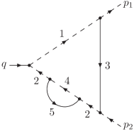
Figure 7: Scalar graph with fermion self-energy

$$F_{\mathrm{fc}}(n_{1},\ldots,n_{5})=e^{2\varepsilon\gamma_{E}}\,(M^{2})^{2\varepsilon}\,(Q^{2})^{n-4}$$

$$\times\int\!\frac{\mathrm{d}^{d}k}{i\pi^{d/2}}\int\!\frac{\mathrm{d}^{d}\ell}{i\pi^{d/2}}\,\frac{1}{(k^{2}+2k\cdot p_{1})^{n_{1}}\,(k^{2}+2k\cdot p_{2})^{n_{2}}}$$

$$\times\frac{1}{(k^{2}-M^{2})^{n_{3}}\,((p_{2}+k+\ell)^{2})^{n_{4}}\,(\ell^{2}-M^{2})^{n_{5}}}\,,$$ (40)

with $k=k_{3}$, $\ell=k_{5}$ and $n=n_{12345}$. For this graph, not every scalar product appearing in the numerator can be expressed linearly in terms of the only five factors in the denominator. But by applying standard tensor reduction Passarino:1978jh to the subgraph of the one-loop self-energy insertion (lines 4 and 5), the formally irreducible scalar products may be transformed into reducible ones, so that only scalar integrals without numerator have to be treated.

Due to the self-energy insertion the evaluation of the loop integrations is rather easy. The complete scalar integral (3.6) with general indices $n_{i}$ may be expressed as an only two-fold Mellin–Barnes representation:

$$F_{\mathrm{fc}}(n_{1},\ldots,n_{5})=\frac{e^{-ni\pi}\,e^{2\varepsilon\gamma_{E}}\,\Gamma(\frac{d}{2}-n_{4})}{\Gamma(n_{1})\Gamma(n_{3})\Gamma(n_{4})\Gamma(n_{5})}$$

$$\times\int_{-i\infty}^{i\infty}\!\frac{\mathrm{d}z_{1}}{2\pi i}\int_{-i\infty}^{i\infty}\!\frac{\mathrm{d}z_{2}}{2\pi i}\,\left(\frac{M^{2}}{Q^{2}}\right)^{2\varepsilon+z_{1}}\,\frac{\Gamma(d-n_{2345}-z_{1})}{\Gamma(\frac{3}{2}d-n_{12345}-z_{1})}$$

$$\times\Gamma(n_{12345}-d+z_{1})\,\Gamma(-z_{2})\Gamma(n_{3}+z_{2})\Gamma(\tfrac{d}{2}-n_{1}+z_{2})$$

$$\times\frac{\Gamma(-n_{3}-z_{1}-z_{2})\Gamma(\frac{d}{2}-n_{35}-z_{1}-z_{2})}{\Gamma(d-n_{345}-z_{1}-z_{2})}$$

$$\times\frac{\Gamma(n_{345}-\frac{d}{2}+z_{1}+z_{2})}{\Gamma(n_{2345}-\frac{d}{2}+z_{1}+z_{2})}\,.$$ (41)

From this expression, the residues producing non-suppressed contributions are extracted. They correspond exactly to the contributions from the following five regions:

(h-h): $$k\sim Q,\quad \ell\sim Q$$

(1c-h): $$k\;\|\;p_{1}, \ell\sim Q$$

(2c-2c): $$k\;\|\;p_{2}, \ell\;\|\;p_{2}$$

(h-s): $$k\sim Q, \ell\sim M$$

(1c-s): $$k\;\|\;p_{1}, \ell\sim M$$

These contributions are evaluated as

$$F_{\mathrm{fc}}^{\text{(h-h)}}(n_{1},\ldots,n_{5})=\left(\frac{M^{2}}{Q^{2}}\right)^{2\varepsilon}\,e^{-ni\pi}\,e^{2\varepsilon\gamma_{E}}$$

$$\times\frac{\Gamma(\frac{d}{2}-n_{13})\Gamma(\frac{d}{2}-n_{4})\Gamma(\frac{d}{2}-n_{5})\Gamma(d-n_{2345})}{\Gamma(n_{1})\Gamma(n_{4})\Gamma(n_{5})\Gamma(d-n_{45})\Gamma(\frac{3}{2}d-n_{12345})}$$

$$\times\frac{\Gamma(n_{45}-\frac{d}{2})\Gamma(n_{12345}-d)}{\Gamma(n_{245}-\frac{d}{2})}\,,$$ (42)

$$F_{\mathrm{fc}}^{\text{(1c-h)}}(n_{1},\ldots,n_{5})=\left(\frac{M^{2}}{Q^{2}}\right)^{2-n_{13}+\varepsilon}\,e^{-ni\pi}\,e^{2\varepsilon\gamma_{E}}$$

$$\times\frac{\Gamma(\frac{d}{2}-n_{1})\Gamma(\frac{d}{2}-n_{4})\Gamma(\frac{d}{2}-n_{5})\Gamma(\frac{d}{2}+n_{1}-n_{245})}{\Gamma(n_{1})\Gamma(n_{3})\Gamma(n_{4})\Gamma(n_{5})\Gamma(d-n_{45})\Gamma(d-n_{245})}$$

$$\times\Gamma(n_{13}-\tfrac{d}{2})\Gamma(n_{45}-\tfrac{d}{2})\,,$$ (43)

$$F_{\mathrm{fc}}^{\text{(2c-2c)}}(n_{1},\ldots,n_{5})=\left(\frac{M^{2}}{Q^{2}}\right)^{4-n_{2345}}\,e^{-ni\pi}\,e^{2\varepsilon\gamma_{E}}$$

$$\times\frac{\Gamma(\frac{d}{2}-n_{4})}{\Gamma(n_{3})\Gamma(n_{4})\Gamma(n_{5})\Gamma(\frac{d}{2}-n_{1})}\int_{-i\infty}^{i\infty}\!\frac{\mathrm{d}z}{2\pi i}\,\frac{\Gamma(-z)}{\Gamma(n_{2}-z)}$$

$$\times\Gamma(n_{24}-\tfrac{d}{2}-z)\Gamma(n_{245}-d-z)\,\Gamma(n_{3}+z)$$

$$\times\frac{\Gamma(\frac{d}{2}-n_{1}+z)\Gamma(\frac{d}{2}-n_{2}+z)}{\Gamma(\frac{d}{2}+z)}\,,$$ (44)

$$F_{\mathrm{fc}}^{\text{(h-s)}}(n_{1},\ldots,n_{5})=\left(\frac{M^{2}}{Q^{2}}\right)^{2-n_{5}+\varepsilon}\,e^{-ni\pi}\,e^{2\varepsilon\gamma_{E}}$$

$$\times\frac{\Gamma(\frac{d}{2}-n_{13})\Gamma(\frac{d}{2}-n_{234})\Gamma(n_{1234}-\frac{d}{2})\Gamma(n_{5}-\frac{d}{2})}{\Gamma(n_{1})\Gamma(n_{5})\Gamma(n_{24})\Gamma(d-n_{1234})}\,,$$ (45)

$$F_{\mathrm{fc}}^{\text{(1c-s)}}(n_{1},\ldots,n_{5})=\left(\frac{M^{2}}{Q^{2}}\right)^{4-n_{135}}\,e^{-ni\pi}\,e^{2\varepsilon\gamma_{E}}$$

$$\times\frac{\Gamma(n_{1}-n_{24})\Gamma(\frac{d}{2}-n_{1})\Gamma(n_{13}-\frac{d}{2})\Gamma(n_{5}-\frac{d}{2})}{\Gamma(n_{1})\Gamma(n_{3})\Gamma(n_{5})\Gamma(\frac{d}{2}-n_{24})}\,.$$ (46)

The contribution of the (h-h) region is known from the massless diagram Kramer:1986sg ; Kramer:1986sgE ; Matsuura:1988sm ; Gonsalves:1983nq . In the reduction to scalar integrals only parameters $n_{i}$ with $n_{2}\leq 2$ and $n_{i}\leq 1$, $i=1,3,4,5$, are involved. Therefore the contributions of the (h-s) and (1c-s) regions are always suppressed by at least one factor $M^{2}/Q^{2}$. On the other hand, the (2c-2c) region is of order $(M^{2}/Q^{2})^{-1}$ if $n_{2}=2$, $n_{3}=n_{4}=n_{5}=1$, but this inverse power of $M^{2}$ is cancelled by a factor of $M^{2}$ from the reduction to scalar integrals.

For the leading order in $M^{2}/Q^{2}$, no analytic regularization is necessary. The contributions of the (h-h), (1c-h) and (2c-2c) regions sum up to the results for the scalar integrals, e.g.

$$F_{\mathrm{fc}}(1,1,1,1,1) =\frac{1}{\varepsilon}\left(-\frac{1}{2}\mathcal{L}^{2}-\frac{\pi^{2}}{3}\right)+\frac{1}{2}\mathcal{L}^{3}-\mathcal{L}^{2}$$

$$\qquad+4\zeta_{3}-\frac{\pi^{2}}{3}\,,$$ (47)

$$F_{\mathrm{fc}}(1,2,1,1,1) =\frac{Q^{2}}{M^{2}}\,\biggl{[}-\frac{1}{\varepsilon^{2}}-\frac{1}{\varepsilon}-\frac{\pi^{2}}{3}-\frac{3}{2}\biggr{]}\,.$$ (48)

The whole vertex correction originating from the Feynman diagram in figure 2d) evaluates to

$$F_{\mathrm{v},\mathrm{fc}} =C_{F}^{2}\left(\frac{\alpha}{4\pi}\right)^{2}\left(\frac{\mu^{2}}{M^{2}}\right)^{2\varepsilon}S_{\varepsilon}^{2}\,\Biggl{\{}-\frac{1}{2\varepsilon^{2}}$$

$$\qquad+\frac{1}{\varepsilon}\left[\mathcal{L}^{2}-3\mathcal{L}+\frac{2}{3}\pi^{2}+\frac{13}{4}\right]-\mathcal{L}^{3}+5\mathcal{L}^{2}$$

$$\qquad-\frac{33}{2}\mathcal{L}-8\zeta_{3}-\frac{\pi^{2}}{4}+\frac{171}{8}\Biggr{\}}+\mathcal{O}(\varepsilon)+\mathcal{O}\!\left(\frac{M^{2}}{Q^{2}}\right).$$ (49)

3.7 Vertex correction with non-Abelian Mercedes–Benz graph

The Mercedes–Benz graph in figure 3a) is of pure non-Abelian nature due to its three-gauge-boson vertex. The corresponding scalar integrals are illustrated in figure 8

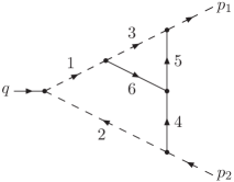
Figure 8: Scalar non-Abelian Mercedes–Benz graph

and defined as follows:

$$F_{\mathrm{BE}C_{\!A}}(n_{1},\ldots,n_{7})=e^{2\varepsilon\gamma_{E}}\,(M^{2})^{2\varepsilon}\,(Q^{2})^{n-n_{7}-4}$$

$$\times\int\!\frac{\mathrm{d}^{d}k}{i\pi^{d/2}}\int\!\frac{\mathrm{d}^{d}\ell}{i\pi^{d/2}}\,\frac{(2p_{2}\cdot k)^{n_{7}}}{(\ell^{2}-2p_{1}\cdot\ell)^{n_{1}}\,(\ell^{2}-2p_{2}\cdot\ell)^{n_{2}}}$$

$$\times\frac{1}{(k^{2}-2p_{1}\cdot k)^{n_{3}}\,(\ell^{2}-M^{2})^{n_{4}}\,(k^{2}-M^{2})^{n_{5}}}$$

$$\times\frac{1}{((k-\ell)^{2}-M^{2})^{n_{6}}}\,,$$ (50)

with $k=k_{5}$, $\ell=k_{4}$ and $n=n_{123456}$. This definition is the same as for the Abelian Mercedes–Benz graph in figure 6 and equation (3.5), except for the distribution of the masses in the propagators. Also the list of relevant regions is similar, but now there is the (s’-h) region instead of the (us-2c) region:

(h-h): $$k\sim Q,\quad \ell\sim Q$$

(1c-h): $$k\;\|\;p_{1}, \ell\sim Q$$

(h-2c): $$k\sim Q, \ell\;\|\;p_{2}$$

(s’-h): $$k_{6}\sim M,\quad \ell\sim Q$$

(1c-1c): $$k\;\|\;p_{1}, \ell\;\|\;p_{1}$$

(2c-2c): $$k\;\|\;p_{2}, \ell\;\|\;p_{2}$$

(1c-2c): $$k\;\|\;p_{1}, \ell\;\|\;p_{2}$$

The (s’-h) region is of order $(M^{2}/Q^{2})^{2-n_{6}+\varepsilon}$ and therefore suppressed with respect to the (h-h) region, as $n_{i}\leq 1$ ($i=1,\ldots,6$). The (2c-2c) region is of order $(M^{2}/Q^{2})^{4-n_{2456}+n_{7}}$ and suppressed for $n_{7}>0$; it is only evaluated for $n_{7}=0$.

The leading contributions of regions with $k_{3},k_{5},k_{6}\sim Q$ are identical to the corresponding contributions of the Abelian Mercedes–Benz graph:

$$F_{\mathrm{BE}C_{\!A}}^{\text{(h-h)}}(n_{1},\ldots,n_{7}) =F_{\mathrm{BE}}^{\text{(h-h)}}(n_{1},\ldots,n_{7})\,,$$ (51)

$$F_{\mathrm{BE}C_{\!A}}^{\text{(h-2c)}}(n_{1},\ldots,n_{7}) =F_{\mathrm{BE}}^{\text{(h-2c)}}(n_{1},\ldots,n_{7})\,.$$ (52)

The contributions of the other regions are given by

$$F_{\mathrm{BE}C_{\!A}}^{\text{(1c-h)}}(n_{1},\ldots,n_{7})=\left(\frac{M^{2}}{Q^{2}}\right)^{2-n_{35}+\varepsilon}\,e^{-ni\pi}\,e^{2\varepsilon\gamma_{E}}$$

$$\times\frac{\Gamma(\frac{d}{2}-n_{3})\Gamma(\frac{d}{2}-n_{146})\Gamma(n_{35}-\frac{d}{2})}{\Gamma(n_{1})\Gamma(n_{2})\Gamma(n_{3})\Gamma(n_{5})\Gamma(n_{6})\Gamma(d-n_{1246})}$$

$$\times\int_{-i\infty}^{i\infty}\!\frac{\mathrm{d}z}{2\pi i}\,\frac{\Gamma(-z)\Gamma(\frac{d}{2}-n_{246}-z)\Gamma(n_{6}+z)\Gamma(n_{37}+z)}{\Gamma(\frac{d}{2}+n_{7}+z)}$$

$$\times\Gamma(n_{1246}-\tfrac{d}{2}+z)\,,$$ (53)

$$F_{\mathrm{BE}C_{\!A}}^{\text{(1c-1c)}}(n_{1},\ldots,n_{7})=\left(\frac{M^{2}}{Q^{2}}\right)^{4-n_{13456}}\,e^{-ni\pi}\,e^{2\varepsilon\gamma_{E}}$$

$$\times\sum_{i_{1},i_{2},i_{3}\geq 0}^{i_{123}\leq n_{7}}\frac{n_{7}!}{i_{1}!\,i_{2}!\,i_{3}!\,(n_{7}-i_{123})!}\,\frac{\Gamma(n_{17}-i_{12})}{\Gamma(n_{1})\Gamma(n_{3})\Gamma(n_{4})\Gamma(n_{5})}$$

$$\times\frac{1}{\Gamma(n_{6})\Gamma(\frac{d}{2}-n_{2}+n_{7})}\int_{-i\infty}^{i\infty}\!\frac{\mathrm{d}z_{1}}{2\pi i}\int_{-i\infty}^{i\infty}\!\frac{\mathrm{d}z_{2}}{2\pi i}\,\Gamma(-z_{1})\Gamma(-z_{2})$$

$$\times\Gamma(n_{5}+z_{1})\Gamma(\tfrac{d}{2}-n_{3}+n_{7}-i_{123}+z_{1})\Gamma(n_{4}+i_{1}+z_{2})$$

$$\times\frac{\Gamma(n_{1467}-i_{123}-\tfrac{d}{2}+z_{2})\Gamma(n_{13456}-d+z_{2})}{\Gamma(n_{147}-i_{2}+z_{2})}$$

$$\times\frac{\Gamma(n_{134}+i_{13}-\tfrac{d}{2}-z_{1}+z_{2})}{\Gamma(n_{14567}-i_{123}-\frac{d}{2}+z_{1}+z_{2})}$$

$$\times\frac{\Gamma(\frac{d}{2}-n_{14}+i_{2}+z_{1}-z_{2})}{\Gamma(\frac{d}{2}-n_{4}+n_{7}-i_{1}+z_{1}-z_{2})}$$

$$\times\Gamma(\tfrac{d}{2}-n_{24}+n_{7}-i_{1}+z_{1}-z_{2})\,,$$ (54)

$$F_{\mathrm{BE}C_{\!A}}^{\text{(2c-2c)}}(n_{1},\ldots,n_{6},n_{7}=0)=\left(\frac{M^{2}}{Q^{2}}\right)^{4-n_{2456}}\,e^{-ni\pi}\,e^{2\varepsilon\gamma_{E}}$$

$$\times\frac{\Gamma(n_{2}-n_{13})}{\Gamma(n_{2})\Gamma(n_{4})\Gamma(n_{5})\Gamma(n_{6})\Gamma(\frac{d}{2}-n_{13})}\int_{-i\infty}^{i\infty}\!\frac{\mathrm{d}z}{2\pi i}\,\Gamma(-z)$$

$$\times\frac{\Gamma(n_{24}-\frac{d}{2}-z)\Gamma(n_{5}+z)\Gamma(n_{6}-n_{3}+z)}{\Gamma(n_{56}-n_{3}+2z)}$$

$$\times\Gamma(\tfrac{d}{2}-n_{2}+z)\Gamma(n_{56}-\tfrac{d}{2}+z)\,,$$ (55)

$$F_{\mathrm{BE}C_{\!A}}^{\text{(1c-2c)}}(n_{1},\ldots,n_{7})=\left(\frac{M^{2}}{Q^{2}}\right)^{4-n_{2345}}\,e^{-ni\pi}\,e^{2\varepsilon\gamma_{E}}$$

$$\times\frac{\Gamma(n_{2}-n_{16})\Gamma(n_{37}-n_{6})\Gamma(\frac{d}{2}-n_{2})\Gamma(\frac{d}{2}-n_{3})}{\Gamma(n_{2})\Gamma(n_{3})\Gamma(n_{4})\Gamma(n_{5})\Gamma(\frac{d}{2}-n_{16})\Gamma(\frac{d}{2}-n_{6}+n_{7})}$$

$$\times\Gamma(n_{24}-\tfrac{d}{2})\Gamma(n_{35}-\tfrac{d}{2})\,.$$ (56)

The evaluation of this non-Abelian vertex graph is more complicated than in the Abelian case, mainly due to the appearance of three massive propagators. The complete summation of the infinite number of residues in the Mellin–Barnes integrals (3.7) and (3.7) is quite intricate. As the calculation of the four-fermion amplitude demands the result of the form factor only to N³LL accuracy, we have refrained from calculating the non-logarithmic constant in the non-Abelian corrections (cf. the beginning of section 3). Therefore we have only extracted all logarithms $\ln(Q^{2}/M^{2})$ from the integrals.

The (1c-h) region has been evaluated in the usual way as described in the previous sections. From the (c-c) regions, i.e. (1c-1c), (2c-2c) and (1c-2c), the logarithmic contributions have been isolated. The expressions for the regions depend on $M^{2}/Q^{2}$ only through a prefactor of the form $(M^{2}/Q^{2})^{m+x}$, where $m$ is an integer and $x$ is made up of regularization parameters (like $\varepsilon$) tending to zero. Logarithms $\ln(Q^{2}/M^{2})$ arise only when poles in the regularization parameters appear, e.g.

$$\left(\frac{M^{2}}{Q^{2}}\right)^{x}\,\frac{1}{x}=\frac{1}{x}-\ln\!\left(\frac{Q^{2}}{M^{2}}\right)+\mathcal{O}(x)\,.$$

As the exponents of these prefactors in the contributions (3.7)–(3.7) of the (c-c) regions involve only the parameters $n_{i}$ and not $\varepsilon$, only poles originating from the analytic regularization may give rise to logarithms. A thorough analysis of the Mellin–Barnes integrals shows that such poles only appear in the following seven integrals:

$$F_{\mathrm{BE}C_{\!A}}^{\text{(}c-c)}(-1,1,1,1,1,1,0)\,,$$

$$F_{\mathrm{BE}C_{\!A}}^{\text{(}c-c)}(0,1,1,1,1,1,n_{7})\,\quad\text{with $n_{7}=0,1,2$},$$

$$F_{\mathrm{BE}C_{\!A}}^{\text{(}c-c)}(1,1,0,1,1,1,0)\,\quad\text{and}$$

$$F_{\mathrm{BE}C_{\!A}}^{\text{(}c-c)}(1,1,1,1,1,0,n_{7})\,\quad\text{with $n_{7}=0,1$}.$$

When closing the integration contours in the Mellin–Barnes integrals, it is sufficient to take those residues which are responsable for the poles. In most cases these are only a finite number of residues. Only the integrals $F_{\mathrm{BE}C_{\!A}}^{\text{(}c-c)}(0,1,1,1,1,1,0)$ and $F_{\mathrm{BE}C_{\!A}}^{\text{(}c-c)}(1,1,0,1,1,1,0)$ need the summation of an infinite number of residues. Such summations can be transformed to infinite series like

$$\sum_{m=0}^{\infty}\frac{1}{\binom{2m}{m}}\left(\frac{1}{3+2m}-\frac{1}{1+2m}\right)\\ \times\left(\frac{1}{3+2m}+\frac{1}{1+2m}+S_{1}(2m)-S_{1}(m)\right),$$ (57)

where $S_{1}(m)=\sum_{i=1}^{m}\frac{1}{i}$ is a harmonic sum. Recently there has been a lot of progess in solving summations like (57) analytically (see e.g. Moch:2001zr ; Weinzierl:2004bn ). But still not all possible cases are covered, and the transformation of a given expression into a series where the solution is known can be quite cumbersome.

On the other hand, the series in (57) is converging very fast. The numerical summation of the first 300 terms approximates the series with an accuracy of more than 100 decimal digits. This enables us to use the following method (see e.g. Kalmykov:2000qe ). An ansatz is chosen as a linear combination of analytical constants like $\pi^{2}$, $\zeta_{3}$, $\ln^{4}2$ etc. with unknown rational coefficients. The determination of the coefficients starting from the numerical result is performed by the PSLQ algorithm Ferguson:1991 ; Bailey:1993 ; Ferguson:1996 . We have used an implementation Veretin:PSLQ of PSLQ in Fortran with multiprecision arithmetic Bailey:1990 ; Bailey:1991 . The series above in (57) has hereby been identified with the analytical expression $4\sqrt{3}\,\mathrm{Cl}_{2}(\tfrac{\pi}{3})-8$, where $\mathrm{Cl}_{2}(\frac{\pi}{3})\approx 1.014942$ is a value of the Clausen function.

In addition to the logarithms, we have calculated in a purely analytical way the complete set of poles in $\varepsilon$ in order to control the cancellation of ultraviolet and infrared singularities.

The contributions from all regions sum up to the results of the scalar integrals, from which we quote the two most complicated ones:

$$F_{\mathrm{BE}C_{\!A}}(0,1,1,1,1,1,0) =-\frac{1}{12}\mathcal{L}^{4}-\frac{\pi^{2}}{6}\mathcal{L}^{2}+\frac{2}{3}\zeta_{3}\mathcal{L}\,,$$ (58)

$$F_{\mathrm{BE}C_{\!A}}(1,1,0,1,1,1,0) =\frac{1}{\varepsilon}\left(-\frac{1}{2}\mathcal{L}^{2}-\frac{\pi^{2}}{3}\right)+\frac{1}{3}\mathcal{L}^{3}-\mathcal{L}^{2}$$

$$\qquad+2\sqrt{3}\mathrm{Cl}_{2}\!\left(\frac{\pi}{3}\right)\mathcal{L}\,,$$ (59)

where non-logarithmic terms of order $\varepsilon^{0}$ have been omitted. The integrals $F_{\mathrm{BE}C_{\!A}}(1,n_{2},1,1,1,1,n_{7})$ are of order $(M^{2}/Q^{2})^{-1}$, with the only contribution coming from the (1c-1c) region, and the inverse power of $M^{2}$ is again cancelled by a factor of $M^{2}$ from the reduction to scalar integrals. These integrals, however, produce neither logarithms $\mathcal{L}=\ln(Q^{2}/M^{2})$ nor poles in $\varepsilon$ and do therefore not contribute to the result in N³LL accuracy. The result for the vertex correction corresponding to the non-Abelian Mercedes–Benz graph in figure 3a) is as follows:

$$F_{\mathrm{v},{\mathrm{BE}C_{\!A}}} =C_{F}C_{A}\left(\frac{\alpha}{4\pi}\right)^{2}\left(\frac{\mu^{2}}{M^{2}}\right)^{2\varepsilon}S_{\varepsilon}^{2}\,\Biggl{\{}\frac{3}{4\varepsilon^{2}}$$

$$\qquad+\frac{1}{\varepsilon}\left[-\frac{3}{2}\mathcal{L}^{2}+\frac{9}{2}\mathcal{L}-\pi^{2}-\frac{37}{8}\right]+\frac{1}{12}\mathcal{L}^{4}$$

$$\qquad+\frac{1}{2}\mathcal{L}^{3}+\left(\frac{\pi^{2}}{6}-\frac{11}{2}\right)\mathcal{L}^{2}$$

$$\qquad+\left(4\sqrt{3}\,\mathrm{Cl}_{2}\!\left(\frac{\pi}{3}\right)-\frac{2}{3}\zeta_{3}-\frac{5}{6}\pi^{2}+\frac{89}{4}\right)\mathcal{L}\Biggr{\}}$$

$$\quad+\mathcal{O}(\varepsilon^{0}\mathcal{L}^{0})+\mathcal{O}(\varepsilon)+\mathcal{O}\!\left(\frac{M^{2}}{Q^{2}}\right).$$ (60)

3.8 Non-Abelian vertex corrections with loop insertions

This section treats all vertex diagrams from figure 3 where a self-energy loop has been inserted in the gauge boson propagator: the gauge boson loop in figure 3b), the ghost field loop in figure 3c) and loops involving the Higgs and Goldstone bosons in figures 3d), 3e) and 3f). Care must be taken in the interpretation of the Feynman rules (appendix A) not to forget the factor $(-1)$ for the loop of the anticommuting ghost fields and the symmetry factor $1/2$ for the loops with two gauge bosons or two Goldstone bosons.

Additional contributions from “tadpoles”, where a loop of only one gauge, Higgs or Goldstone boson is attached to the gauge boson propagator via a vertex with four fields, are omitted here because they are cancelled exactly by the corresponding contributions from the renormalization of the gauge boson mass (see section 4).

For the Higgs boson mass $M_{H}$ we use the approximation $M_{H}=M_{W}$, which facilitates the loop calculations. The form factor depends on the Higgs mass only in N³LL accuracy, i.e. via the coefficient of the linear logarithm, and the higher powers of the electroweak logarithm are not affected by changes in the Higgs mass. We have checked explicitly by evaluating the Higgs contributions for the hypothetical case $M_{H}=0$ (see the discussion of the results in section 5) that effects due to a wrong value of the Higgs mass are indeed negligible.

As in our approximation (and using the Feynman–’t Hooft gauge) all particles running in the self-energy loop have the same mass $M=M_{W}$, the vertex corrections of this section share the same set of scalar integrals, which are illustrated in figure 9

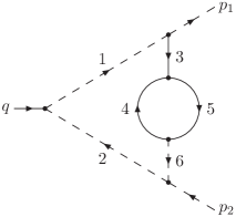
Figure 9: Scalar graph for non-Abelian vertex corrections with loop insertions

and defined in the following equation:

$$F_{\mathrm{Wc}}(n_{1},\ldots,n_{6})=e^{2\varepsilon\gamma_{E}}\,(M^{2})^{2\varepsilon}\,(Q^{2})^{n-4}$$

$$\times\int\!\frac{\mathrm{d}^{d}k}{i\pi^{d/2}}\int\!\frac{\mathrm{d}^{d}\ell}{i\pi^{d/2}}\,\frac{1}{(k^{2}+2p_{1}\cdot k)^{n_{1}}\,(k^{2}+2p_{2}\cdot k)^{n_{2}}}$$

$$\times\frac{1}{(k^{2}-M^{2})^{n_{3}}\,(\ell^{2}-M^{2})^{n_{4}}\,((k+\ell)^{2}-M^{2})^{n_{5}}\,(k^{2})^{n_{6}}}\,,$$ (61)

with $k=k_{3}$ and $\ell=k_{4}$. The additional massless propagator corresponding to the parameter $n_{6}$ is introduced when performing a tensor reduction on the self-energy loop (lines 4 and 5) in order to eliminate the scalar products in the numerator of the integral. The presence of both a massive and a massless propagator with the same momentum $k_{3}=k_{6}=k$ could, of course, be avoided by partial fractioning. But this would produce factors of $1/M^{2}$, complicating the expansion in $M^{2}/Q^{2}$. So we remained with both propagators in the scalar integrals (3.8). In order to avoid ambiguities in the reduction to scalar integrals, we fixed $n_{3}=2$ and cancelled factors of $k^{2}$ in the numerator exclusively with the sixth propagator.

In general the following regions are relevant:

(h-h): $$k\sim Q,\quad \ell\sim Q$$

(h-s): $$k\sim Q, \ell\sim M$$

(h-s’): $$k\sim Q, k_{5}\sim M$$

(1c-1c): $$k\;\|\;p_{1}, \ell\;\|\;p_{1}$$

(2c-2c): $$k\;\|\;p_{2}, \ell\;\|\;p_{2}$$

But since the (h-s) regions is of order $(M^{2}/Q^{2})^{2-n_{4}+\varepsilon}$ and the (h-s’) regions is of order $(M^{2}/Q^{2})^{2-n_{5}+\varepsilon}$, they are both suppressed with respect to the (h-h) region for all relevant cases. The contributions from the other regions can be expressed as follows:

$$F_{\mathrm{Wc}}^{\text{(h-h)}}(n_{1},\ldots,n_{6})=\left(\frac{M^{2}}{Q^{2}}\right)^{2\varepsilon}\,e^{-ni\pi}\,e^{2\varepsilon\gamma_{E}}$$

$$\times\frac{\Gamma(\frac{d}{2}-n_{4})\Gamma(\frac{d}{2}-n_{5})\Gamma(d-n_{13456})\Gamma(d-n_{23456})}{\Gamma(n_{1})\Gamma(n_{2})\Gamma(n_{4})\Gamma(n_{5})\Gamma(d-n_{45})\Gamma(\frac{3}{2}d-n_{123456})}$$

$$\times\Gamma(n_{45}-\tfrac{d}{2})\Gamma(n_{123456}-d)\,,$$ (62)

$$F_{\mathrm{Wc}}^{\text{(1c-1c)}}(n_{1},\ldots,n_{6})=\left(\frac{M^{2}}{Q^{2}}\right)^{4-n_{13456}}\,e^{-ni\pi}\,e^{2\varepsilon\gamma_{E}}$$

$$\times\frac{\Gamma(n_{1}-n_{2})}{\Gamma(n_{1})\Gamma(n_{3})\Gamma(n_{4})\Gamma(n_{5})\Gamma(\frac{d}{2}-n_{2})}\,\int_{-i\infty}^{i\infty}\!\frac{\mathrm{d}z}{2\pi i}\,\Gamma(-z)$$

$$\times\frac{\Gamma(n_{136}-\frac{d}{2}-z)\Gamma(n_{4}+z)\Gamma(n_{5}+z)\Gamma(\frac{d}{2}-n_{16}+z)}{\Gamma(n_{45}+2z)}$$

$$\times\Gamma(n_{45}-\tfrac{d}{2}+z)\,.$$ (63)

For symmetry reasons, $F_{\mathrm{Wc}}^{\text{(2c-2c)}}$ can be obtained from $F_{\mathrm{Wc}}^{\text{(1c-1c)}}$ by exchanging $n_{1}\leftrightarrow n_{2}$. Some of the (1c-1c) and (2c-2c) contributions are of order $(M^{2}/Q^{2})^{-1}$, but this inverse power of $M^{2}$ is always cancelled by a factor of $M^{2}$ originating either from the reduction to scalar integrals or from the Feynman rules, when two $WWH$-vertices are present.

As for the non-Abelian Mercedes–Benz graph in the previous section, we have only extracted the logarithms and the poles in $\varepsilon$. The (c-c) regions (1c-1c) and (2c-2c) produce logarithmic terms for $n_{1}=n_{2}=1$. For most of the (c-c) contributions, the evaluation of a finite number of residues in the complex $z$-plane is sufficient. Only the two cases $F_{\mathrm{Wc}}^{\text{(c-c)}}(1,1,2,1,1,0)$ and $F_{\mathrm{Wc}}^{\text{(c-c)}}(1,1,2,1,1,-1)$ demand the summation of an infinite number of residues. We have solved these two summations numerically and found the corresponding analytic expressions with the help of the PSLQ algorithm. In all cases the extraction of the poles in $\varepsilon$ required only a finite number of residues.

We quote the results for the two most complicated scalar integrals:

$$\!\!F_{\mathrm{Wc}}(1,1,2,1,1,0)=\frac{Q^{2}}{M^{2}}\,\biggl{[}\frac{1}{\varepsilon}-\frac{4}{3}\sqrt{3}\mathrm{Cl}_{2}\!\left(\frac{\pi}{3}\right)+2\biggr{]}\,\mathcal{L}\,,$$ (64)

$$\!\!F_{\mathrm{Wc}}(1,1,2,1,1,-1)=\frac{1}{\varepsilon}\left(-\frac{1}{2}\mathcal{L}^{2}+\mathcal{L}-\frac{\pi^{2}}{3}\right)+\frac{1}{3}\mathcal{L}^{3}$$

$$-\mathcal{L}^{2}+\left(\frac{2}{3}\sqrt{3}\mathrm{Cl}_{2}\!\left(\frac{\pi}{3}\right)+2\right)\mathcal{L}\,.$$ (65)

The vertex corrections corresponding to the Feynman diagrams in figures 3b)–3f) are obtained by inserting the results for the scalar integrals into the expressions returned from the reduction of each diagram.

The vertex corrections with the non-Abelian gauge boson and ghost field loops, figures 3b) and 3c), have been evaluated together. Their sum is

$$F_{\mathrm{v},{W\!W\!cc}} =C_{F}C_{A}\left(\frac{\alpha}{4\pi}\right)^{2}\left(\frac{\mu^{2}}{M^{2}}\right)^{2\varepsilon}S_{\varepsilon}^{2}\,\Biggl{\{}$$

$$\qquad\frac{1}{\varepsilon}\left[-\frac{5}{3}\mathcal{L}^{2}+\frac{49}{3}\mathcal{L}-\frac{10}{9}\pi^{2}-\frac{337}{12}\right]+\frac{10}{9}\mathcal{L}^{3}$$

$$\qquad-\frac{76}{9}\mathcal{L}^{2}+\left(-4\sqrt{3}\,\mathrm{Cl}_{2}\!\left(\frac{\pi}{3}\right)+\frac{859}{18}\right)\mathcal{L}\Biggr{\}}$$

$$\quad+\mathcal{O}(\varepsilon^{0}\mathcal{L}^{0})+\mathcal{O}(\varepsilon)+\mathcal{O}\!\left(\frac{M^{2}}{Q^{2}}\right).$$ (66)

The vertex correction in figure 3d) with gauge and Higgs boson in the loop insertion contains two factors of $M$ from the two $WWH$-vertices, but these are cancelled by factors $1/M^{2}$ in the results of some of the scalar integrals. So this vertex correction is not suppressed:

$$F_{\mathrm{v},{W\!H}} =\left(\frac{\alpha}{4\pi}\right)^{2}\left(\frac{\mu^{2}}{M^{2}}\right)^{2\varepsilon}S_{\varepsilon}^{2}\,\Biggl{\{}\frac{1}{\varepsilon}\left[-\frac{3}{2}\mathcal{L}+3\right]$$

$$\qquad+\biggl{(}2\sqrt{3}\,\mathrm{Cl}_{2}\!\left(\frac{\pi}{3}\right)-3\biggr{)}\,\mathcal{L}\Biggr{\}}$$

$$\quad+\mathcal{O}(\varepsilon^{0}\mathcal{L}^{0})+\mathcal{O}(\varepsilon)+\mathcal{O}\!\left(\frac{M^{2}}{Q^{2}}\right).$$ (67)

The two vertex corrections in figures 3e) and 3f) with Higgs and Goldstone bosons in the loop insertion yield the same result (for $M_{H}=M$):

$$F_{\mathrm{v},{H\!\phi}} =F_{\mathrm{v},{\phi\phi}}=\left(\frac{\alpha}{4\pi}\right)^{2}\left(\frac{\mu^{2}}{M^{2}}\right)^{2\varepsilon}S_{\varepsilon}^{2}\,\Biggl{\{}$$

$$\qquad\frac{1}{\varepsilon}\left[\frac{1}{16}\mathcal{L}^{2}+\frac{7}{16}\mathcal{L}+\frac{\pi^{2}}{24}-\frac{67}{64}\right]-\frac{1}{24}\mathcal{L}^{3}$$

$$\qquad+\frac{17}{48}\mathcal{L}^{2}+\biggl{(}-\frac{3}{4}\sqrt{3}\,\mathrm{Cl}_{2}\!\left(\frac{\pi}{3}\right)+\frac{19}{96}\biggr{)}\,\mathcal{L}\Biggr{\}}$$

$$\quad+\mathcal{O}(\varepsilon^{0}\mathcal{L}^{0})+\mathcal{O}(\varepsilon)+\mathcal{O}\!\left(\frac{M^{2}}{Q^{2}}\right).$$ (68)

The contributions involving Higgs and Goldstone bosons are only valid for the spontaneously broken $SU(2)$ model, they cannot be transformed e.g. to a $U(1)$ model simply by setting other values for $C_{F}$, $C_{A}$ and $T_{F}$. We have therefore written these contributions with the Casimir operators already replaced by their $SU(2)$ values.

4 Renormalization contributions

Section 3 has treated the evaluation of the vertex corrections which contribute to the Abelian vector form factor. These have been performed with Feynman rules originating from the unrenormalized Lagrangian. Therefore the contributions due to the renormalization of the fields (section 4.1), the coupling constant (section 4.2) and the gauge boson mass (section 4.3) have to be added.

4.1 Field renormalization

The renormalization of the two fermion fields in the Abelian vector current requires the multiplication of the vertex corrections by a factor of $Z_{f}$, where $(Z_{f})^{1/2}$ is the fermion field renormalization constant. On the other hand, $Z_{f}$ is determined by the fermion self-energy corrections $\Sigma$ at on-shell momentum $p^{2}=0$ (for massless fermions). In a perturbative expansion, the field renormalization constant is $Z_{f}=1+\Sigma_{1}+\Sigma_{2}+\mathcal{O}(\alpha^{3})$ and the vertex corrections are $F_{\mathrm{v}}=1+F_{\mathrm{v},1}+F_{\mathrm{v},2}+\mathcal{O}(\alpha^{3})$, where the indices 1 and 2 indicate the one- and two-loop contributions, respectively.

The total Abelian vector form factor up to order $\alpha^{2}$ can be written as

$$F =F_{\mathrm{v}}\cdot Z_{f}$$

$$=1+{}\underbrace{F_{\mathrm{v},1}+\Sigma_{1}}_{\mathcal{O}(\alpha)}{}+{}\underbrace{F_{\mathrm{v},2}+\Sigma_{2}+F_{\mathrm{v},1}\Sigma_{1}}_{\mathcal{O}(\alpha^{2})}{}+\mathcal{O}(\alpha^{3})\,.$$

The two-loop contribution to the form factor is therefore given by

$$F_{2}=F_{\mathrm{v},2}+\Sigma_{2}+F_{\mathrm{v},1}\Sigma_{1}\,,$$ (69)

where $F_{\mathrm{v},2}$ is made up of the contributions calculated in section 3. The one-loop corrections are well known:

$$F_{\mathrm{v},1} =C_{F}\,\frac{\alpha}{4\pi}\left(\frac{\mu^{2}}{M^{2}}\right)^{\varepsilon}S_{\varepsilon}\,\Biggl{\{}\frac{1}{\varepsilon}-\mathcal{L}^{2}+3\mathcal{L}-\frac{2}{3}\pi^{2}-4$$

$$\qquad+\varepsilon\,\biggl{[}\frac{1}{3}\mathcal{L}^{3}-\frac{3}{2}\mathcal{L}^{2}+\left(-\frac{\pi^{2}}{3}+8\right)\mathcal{L}+2\zeta_{3}+\frac{7}{12}\pi^{2}$$

$$\qquad\quad-12\biggr{]}+\varepsilon^{2}\,\biggl{[}-\frac{1}{12}\mathcal{L}^{4}+\frac{1}{2}\mathcal{L}^{3}+\left(\frac{\pi^{2}}{12}-4\right)\mathcal{L}^{2}$$

$$\qquad\quad+\left(-4\zeta_{3}-\frac{\pi^{2}}{4}+16\right)\mathcal{L}-\frac{13}{180}\pi^{4}+\frac{17}{3}\zeta_{3}+\pi^{2}$$

$$\qquad\quad-28\biggr{]}\Biggr{\}}+\mathcal{O}(\varepsilon^{3})+\mathcal{O}\left(\frac{M^{2}}{Q^{2}}\right),$$ (70)

$$\Sigma_{1} =\Sigma_{1}(p^{2}=0)=C_{F}\,\frac{\alpha}{4\pi}\left(\frac{\mu^{2}}{M^{2}}\right)^{\varepsilon}S_{\varepsilon}\,\Biggl{\{}-\frac{1}{\varepsilon}+\frac{1}{2}$$

$$\qquad+\varepsilon\left[-\frac{\pi^{2}}{12}+\frac{1}{4}\right]+\varepsilon^{2}\left[\frac{1}{3}\zeta_{3}+\frac{\pi^{2}}{24}+\frac{1}{8}\right]\Biggr{\}}$$

$$\quad+\mathcal{O}(\varepsilon^{3})\,.$$ (71)

The terms proportional to $\varepsilon$ and $\varepsilon^{2}$ are needed when $F_{\mathrm{v},1}$ and $\Sigma_{1}$ are multiplied by other one-loop contributions containing $1/\varepsilon$-poles from ultraviolet singularities or $1/\varepsilon^{2}$-poles from mass singularities. The sum $F_{1}=F_{\mathrm{v},1}+\Sigma_{1}$ constitutes the one-loop form factor, which is finite at $\varepsilon=0$.

The two-loop self-energy corrections $\Sigma_{2}$ originate from the Feynman diagrams in figures 10, 11 and 12.

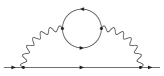
Figure 10: Fermionic self-energy correction

(a)

(b)

(c)

Figure 11: Abelian self-energy corrections

(a)

(b)

(c)

(d)

(e)

(f)

Figure 12: Non-Abelian self-energy corrections

As for the vertex corrections, “tadpole” diagrams are omitted because their contributions are cancelled by the renormalization of the gauge boson mass.

The self-energy amplitudes $\tilde{\Sigma}$ are quadratic matrices both in the spinor and in the isospin space. For massless fermions of momentum $p$ they are of the form

$$\tilde{\Sigma}(p)=-i\makebox[0.0pt][l]{\hskip 3.24997pt\makebox[0.0pt]{/}}p\,\mathbf{1}\,\Sigma(p^{2})\,,$$ (72)

where $\mathbf{1}$ is the unity matrix in the isospin space. The self-energy correction $\Sigma$ may be extracted from the amplitude $\tilde{\Sigma}$ by the projection

$$\Sigma=\frac{i}{4Np^{2}}\,\operatorname{Tr}(\makebox[0.0pt][l]{\hskip 3.24997pt\makebox[0.0pt]{/}}p\tilde{\Sigma})\,,$$ (73)

where $N=2$ for $SU(2)$ and the trace runs over the spinor and the isospin indices. The projection requires $p^{2}\neq 0$, whereas we need the self-energies at $p^{2}=0$. We have therefore calculated the loop integrals for an infinitesimally small, but finite $p^{2}$. By performing the limit $p^{2}\to 0$ before any expansion in $\varepsilon$, no logarithms $\ln(p^{2})$ appear and the first two coefficients of a simple Taylor expansion of the integrals with respect to $p^{2}$ are sufficient. The contribution of every Feynman diagram to the trace in (73) is proportional to $p^{2}$, so no inverse power $1/p^{2}$ is left.

The reduction of the self-energy diagrams to scalar integrals using (73) and the calculation of the integrals was performed similarly to the vertex corrections. In fact, the evaluation of the self-energy corrections is much simpler because they do not depend on $Q^{2}$, only on $M^{2}$, and no expansion by regions is needed. We do not quote further details of this calculation and list only the total results of each Feynman diagram.

The fermionic self-energy correction in figure 10 has already been calculated in Feucht:2003yx :

$$\Sigma_{n_{f}} =C_{F}T_{F}n_{f}\left(\frac{\alpha}{4\pi}\right)^{2}\left(\frac{\mu^{2}}{M^{2}}\right)^{2\varepsilon}S_{\varepsilon}^{2}\left(-\frac{1}{\varepsilon}-\frac{1}{2}\right)+\mathcal{O}(\varepsilon)\,.$$ (74)

The Abelian contributions to the self-energy correction originate from figure 11a),

$$\Sigma_{\mathrm{T1}}=\left(C_{F}^{2}-\frac{1}{2}C_{F}C_{A}\right)\left(\frac{\alpha}{4\pi}\right)^{2}\left(\frac{\mu^{2}}{M^{2}}\right)^{2\varepsilon}S_{\varepsilon}^{2}\\ \times\left(-\frac{1}{\varepsilon^{2}}+\frac{3}{2\varepsilon}-\frac{\pi^{2}}{2}+\frac{7}{4}\right)+\mathcal{O}(\varepsilon)\,,$$ (75)

from figure 11b),

$$\Sigma_{\mathrm{T2}} =C_{F}^{2}\left(\frac{\alpha}{4\pi}\right)^{2}\left(\frac{\mu^{2}}{M^{2}}\right)^{2\varepsilon}S_{\varepsilon}^{2}\left(\frac{1}{2\varepsilon^{2}}-\frac{1}{4\varepsilon}-\frac{\pi^{2}}{12}+\frac{7}{8}\right)$$

$$\quad+\mathcal{O}(\varepsilon)\,,$$ (76)

and from figure 11c), which yields just the square of the one-loop correction (4.1). Only the $C_{F}^{2}$-part of (75) belongs to the Abelian corrections, the $C_{F}C_{A}$-part contributes to the non-Abelian corrections.

The other non-Abelian contributions have been evaluated from figure 12a),

$$\Sigma_{\mathrm{T1}C_{\!A}} =C_{F}C_{A}\left(\frac{\alpha}{4\pi}\right)^{2}\left(\frac{\mu^{2}}{M^{2}}\right)^{2\varepsilon}S_{\varepsilon}^{2}\left(-\frac{3}{2\varepsilon^{2}}-\frac{5}{4\varepsilon}\right)$$

$$\quad+\mathcal{O}(\varepsilon^{0})\,,$$ (77)

from the sum of the diagrams with gauge boson and ghost field loops, figures 12b) and 12c),

$$\Sigma_{W\!W\!cc} =C_{F}C_{A}\left(\frac{\alpha}{4\pi}\right)^{2}\left(\frac{\mu^{2}}{M^{2}}\right)^{2\varepsilon}S_{\varepsilon}^{2}\cdot\frac{21}{4\varepsilon}+\mathcal{O}(\varepsilon^{0})\,,$$ (78)

from figure 12d) with gauge and Higgs boson in the loop insertion,

$$\Sigma_{W\!H} =\left(\frac{\alpha}{4\pi}\right)^{2}\left(\frac{\mu^{2}}{M^{2}}\right)^{2\varepsilon}S_{\varepsilon}^{2}\left(-\frac{3}{4\varepsilon}\right)+\mathcal{O}(\varepsilon^{0})\,,$$ (79)

and, with identical results, from figures 12e) and 12f) with Higgs and Goldstone bosons in the loop insertion,

$$\Sigma_{H\!\phi} =\Sigma_{\phi\phi}=\left(\frac{\alpha}{4\pi}\right)^{2}\left(\frac{\mu^{2}}{M^{2}}\right)^{2\varepsilon}S_{\varepsilon}^{2}\cdot\frac{21}{64\varepsilon}+\mathcal{O}(\varepsilon^{0})\,.$$ (80)

As for the vertex corrections, the Higgs and Goldstone boson contributions have been calculated with the approximation $M_{H}=M$ and are only valid in a spontaneously broken $SU(2)$ model. The evaluation of all non-Abelian contributions has been limited to the poles in $\varepsilon$ because the non-logarithmic finite term of order $\varepsilon^{0}$ has already been neglected in the calculation of the corresponding vertex corrections.

4.2 Coupling constant renormalization

According to the prescription of the $\overline{\text{MS}}$ scheme, the unrenormalized coupling constant $\alpha_{\mathrm{bare}}$ is replaced by the renormalized coupling $\alpha$ via

$$\alpha_{\mathrm{bare}}=\alpha\left(1-\frac{\alpha}{4\pi}\,\frac{\beta_{0}}{\varepsilon}\right)+\mathcal{O}(\alpha^{3})\,,$$ (81)

where $\beta_{0}$ is the one-loop coefficient of the renormalization group $\beta$-function. $\beta_{0}$ gets a non-Abelian contribution proportional to $C_{A}$, a fermionic contribution proportional to $n_{f}$ and a Higgs contribution Gross:1973id ; Politzer:1973fx :

$$\beta_{0}=\frac{11}{3}C_{A}-\frac{4}{3}T_{F}n_{f}-\frac{1}{6}\,.$$ (82)

As mentioned above, the loop calculations have been performed using the unrenormalized Feynman rules. Introducing now the renormalized coupling constant and mass instead of the bare quantities does not change the two-loop results at order $\alpha^{2}$. But the coupling and mass in the one-loop result have to be regarded as the bare parameters and must be replaced by the renormalized ones.

By applying the substitution (81) to the one-loop form factor from equations (4.1) and (4.1), we get additional contributions of order $\alpha^{2}$, namely

$$\Delta F_{C_{A}}^{\alpha} =C_{F}C_{A}\left(\frac{\alpha}{4\pi}\right)^{2}\left(\frac{\mu^{2}}{M^{2}}\right)^{\varepsilon}S_{\varepsilon}\,\Biggl{\{}$$

$$\qquad\frac{1}{\varepsilon}\left[\frac{11}{3}\mathcal{L}^{2}-11\mathcal{L}+\frac{22}{9}\pi^{2}+\frac{77}{6}\right]-\frac{11}{9}\mathcal{L}^{3}$$

$$\qquad+\frac{11}{2}\mathcal{L}^{2}+\left(\frac{11}{9}\pi^{2}-\frac{88}{3}\right)\mathcal{L}-\frac{22}{3}\zeta_{3}-\frac{11}{6}\pi^{2}$$

$$\qquad+\frac{517}{12}\Biggr{\}}+\mathcal{O}(\varepsilon)+\mathcal{O}\!\left(\frac{M^{2}}{Q^{2}}\right),$$ (83)

$$\Delta F_{n_{f}}^{\alpha} =C_{F}T_{F}n_{f}\left(\frac{\alpha}{4\pi}\right)^{2}\left(\frac{\mu^{2}}{M^{2}}\right)^{\varepsilon}S_{\varepsilon}\,\Biggl{\{}$$

$$\qquad\frac{1}{\varepsilon}\left[-\frac{4}{3}\mathcal{L}^{2}+4\mathcal{L}-\frac{8}{9}\pi^{2}-\frac{14}{3}\right]+\frac{4}{9}\mathcal{L}^{3}-2\mathcal{L}^{2}$$

$$\qquad+\left(-\frac{4}{9}\pi^{2}+\frac{32}{3}\right)\mathcal{L}+\frac{8}{3}\zeta_{3}+\frac{2}{3}\pi^{2}-\frac{47}{3}\Biggr{\}}$$

$$\quad+\mathcal{O}(\varepsilon)+\mathcal{O}\!\left(\frac{M^{2}}{Q^{2}}\right),$$ (84)

$$\Delta F_{\mathrm{Higgs}}^{\alpha} =\left(\frac{\alpha}{4\pi}\right)^{2}\left(\frac{\mu^{2}}{M^{2}}\right)^{\varepsilon}S_{\varepsilon}\,\Biggl{\{}$$

$$\qquad\frac{1}{\varepsilon}\left[-\frac{1}{8}\mathcal{L}^{2}+\frac{3}{8}\mathcal{L}-\frac{\pi^{2}}{12}-\frac{7}{16}\right]+\frac{1}{24}\mathcal{L}^{3}$$

$$\qquad-\frac{3}{16}\mathcal{L}^{2}+\left(-\frac{\pi^{2}}{24}+1\right)\mathcal{L}+\frac{1}{4}\zeta_{3}+\frac{\pi^{2}}{16}$$

$$\qquad-\frac{47}{32}\Biggr{\}}+\mathcal{O}(\varepsilon)+\mathcal{O}\!\left(\frac{M^{2}}{Q^{2}}\right).$$ (85)

4.3 Mass renormalization

The relation between the bare gauge boson mass $M_{\mathrm{bare}}$ and the renormalized mass $M$ is determined by the gauge boson self-energy corrections, which have the form

$$\tilde{\Pi}^{\mu\nu,ab}(k)=i\delta^{ab}\,g^{\mu\nu}k^{2}\,\Pi(k^{2})+\text{terms}\propto k^{\mu}k^{\nu}$$ (86)

at momentum $k$. In the on-shell scheme, the square of the physical, renormalized mass is defined to be the real part of the pole of the propagator. At one-loop, the relation between $M_{\mathrm{bare}}$ and $M$ becomes

$$M_{\mathrm{bare}}^{2}=M^{2}\left[1-\operatorname{Re}\Pi_{1}(M^{2})\right]+\mathcal{O}(\alpha^{2})\,,$$ (87)

where $\Pi_{1}$ is the one-loop contribution to $\Pi$. This relation leads to the following substitutions in the one-loop result (4.1) and (4.1):

$$\left(\frac{\mu^{2}}{M^{2}}\right)^{\varepsilon} \to\left(\frac{\mu^{2}}{M^{2}}\right)^{\varepsilon}\left[1+\varepsilon\,\operatorname{Re}\Pi_{1}(M^{2})\right]+\mathcal{O}(\alpha^{2})\,,$$ (88)

$$\mathcal{L}^{n} \to\mathcal{L}^{n}+n\,\mathcal{L}^{n-1}\,\operatorname{Re}\Pi_{1}(M^{2})+\mathcal{O}(\alpha^{2})\,,$$ (89)

with $\mathcal{L}=\ln(Q^{2}/M^{2})$, producing additional contributions of order $\alpha^{2}$.

The one-loop gauge boson self-energy receives contributions from a fermion loop,

$$\Pi_{n_{f}}(M^{2})=T_{F}n_{f}\,\frac{\alpha}{4\pi}\left(\frac{\mu^{2}}{M^{2}}\right)^{\varepsilon}S_{\varepsilon}\left(-\frac{4}{3\varepsilon}-\frac{20}{9}-\frac{4}{3}i\pi\right)\\ +\mathcal{O}(\varepsilon)\,,$$ (90)

from the non-Abelian gauge boson and ghost field loops,

$$\Pi_{W\!W\!cc}(M^{2})=C_{A}\,\frac{\alpha}{4\pi}\left(\frac{\mu^{2}}{M^{2}}\right)^{\varepsilon}S_{\varepsilon}\left(\frac{17}{3\varepsilon}-\frac{4\pi}{\sqrt{3}}+\frac{82}{9}\right)\\ +\mathcal{O}(\varepsilon)\,,$$ (91)

from the loop with gauge and Higgs boson,

$$\Pi_{W\!H}(M^{2})=\frac{\alpha}{4\pi}\left(\frac{\mu^{2}}{M^{2}}\right)^{\varepsilon}S_{\varepsilon}\left(-\frac{1}{\varepsilon}+\frac{\pi}{\sqrt{3}}-2\right)\\ +\mathcal{O}(\varepsilon)\,,$$ (92)

and from the loops with Higgs and Goldstone bosons,

$$\Pi_{H\!\phi}(M^{2})=\Pi_{\phi\phi}(M^{2})=\\ \frac{\alpha}{4\pi}\left(\frac{\mu^{2}}{M^{2}}\right)^{\varepsilon}S_{\varepsilon}\left(\frac{5}{12\varepsilon}-\frac{\pi}{4\sqrt{3}}+\frac{17}{18}\right)+\mathcal{O}(\varepsilon)\,.$$ (93)

The self-energy diagrams with “tadpoles” have been omitted. They do not depend on the momentum of the gauge boson, so their contribution to the mass renormalization cancels exactly the corresponding vertex correction and field renormalization diagrams which have already been dropped out before.

Applying the substitutions (88) and (89) to the one-loop form factor, the self-energy corrections (90)–(93) produce the following contributions to the two-loop form factor:

$$\Delta F_{n_{f}}^{M} =C_{F}T_{F}n_{f}\left(\frac{\alpha}{4\pi}\right)^{2}\left(\frac{\mu^{2}}{M^{2}}\right)^{2\varepsilon}S_{\varepsilon}^{2}\,\Biggl{\{}\frac{1}{\varepsilon}\left[\frac{8}{3}\mathcal{L}-4\right]$$

$$\qquad+\frac{40}{9}\mathcal{L}+\frac{4}{3}\pi^{2}-\frac{38}{3}\Biggr{\}}+\mathcal{O}(\varepsilon)+\mathcal{O}\!\left(\frac{M^{2}}{Q^{2}}\right),$$ (94)

$$\Delta F_{W\!W\!cc}^{M} =C_{F}C_{A}\left(\frac{\alpha}{4\pi}\right)^{2}\left(\frac{\mu^{2}}{M^{2}}\right)^{2\varepsilon}S_{\varepsilon}^{2}\,\Biggl{\{}\frac{1}{\varepsilon}\left[-\frac{34}{3}\mathcal{L}+17\right]$$

$$\qquad+\left(\frac{8\pi}{\sqrt{3}}-\frac{164}{9}\right)\mathcal{L}-4\sqrt{3}\pi-\frac{17}{3}\pi^{2}$$

$$\qquad+\frac{317}{6}\Biggr{\}}+\mathcal{O}(\varepsilon)+\mathcal{O}\!\left(\frac{M^{2}}{Q^{2}}\right),$$ (95)

$$\Delta F_{W\!H}^{M} =\left(\frac{\alpha}{4\pi}\right)^{2}\left(\frac{\mu^{2}}{M^{2}}\right)^{2\varepsilon}S_{\varepsilon}^{2}\,\Biggl{\{}\frac{1}{\varepsilon}\left[\frac{3}{2}\mathcal{L}-\frac{9}{4}\right]$$

$$\qquad+\left(-\frac{1}{2}\sqrt{3}\pi+3\right)\mathcal{L}+\frac{3}{4}\sqrt{3}\pi+\frac{3}{4}\pi^{2}-\frac{63}{8}\Biggr{\}}$$

$$\quad+\mathcal{O}(\varepsilon)+\mathcal{O}\!\left(\frac{M^{2}}{Q^{2}}\right),$$ (96)

$$\Delta F_{H\!\phi}^{M} =\Delta F_{\phi\phi}^{M}=\left(\frac{\alpha}{4\pi}\right)^{2}\left(\frac{\mu^{2}}{M^{2}}\right)^{2\varepsilon}S_{\varepsilon}^{2}\,\Biggl{\{}\frac{1}{\varepsilon}\left[-\frac{5}{8}\mathcal{L}+\frac{15}{16}\right]$$

$$\qquad+\left(\frac{1}{8}\sqrt{3}\pi-\frac{17}{12}\right)\mathcal{L}-\frac{3}{16}\sqrt{3}\pi-\frac{5}{16}\pi^{2}$$

$$\qquad+\frac{113}{32}\Biggr{\}}+\mathcal{O}(\varepsilon)+\mathcal{O}\!\left(\frac{M^{2}}{Q^{2}}\right).$$ (97)

5 Results and discussion

The individual results have been presented in the previous sections so that we can now add them together. According to the $\overline{\text{MS}}$ prescription, the factor $S_{\varepsilon}=(4\pi)^{\varepsilon}e^{-\varepsilon\gamma_{E}}$ is absorbed into $\mu^{2\varepsilon}$ by a redefinition of $\mu$, and we have chosen $\mu=M$ so that the whole prefactor $(\mu^{2}/M^{2})^{\varepsilon}S_{\varepsilon}$ or $(\mu^{2}/M^{2})^{2\varepsilon}S_{\varepsilon}^{2}$ is replaced by 1. The dependence of the form factor on $\mu$ can easily be restored by looking at the running of the coupling $\alpha$, parametrized by $\beta_{0}$, in the one-loop form factor. We give the results in $d=4$ dimensions ($\varepsilon=0$) in the Sudakov limit $Q^{2}\gg M^{2}$.

The fermionic contribution to the Abelian vector form factor is obtained from equations (3.2), (74), (4.2) and (4.3) Feucht:2003yx :

$$F_{2,n_{f}} =F_{\mathrm{v},n_{f}}+\Sigma_{n_{f}}+\Delta F_{n_{f}}^{\alpha}+\Delta F_{n_{f}}^{M}$$

$$=C_{F}T_{F}n_{f}\left(\frac{\alpha}{4\pi}\right)^{2}\,\biggl{\{}-\frac{4}{9}\mathcal{L}^{3}+\frac{38}{9}\mathcal{L}^{2}-\frac{34}{3}\mathcal{L}$$

$$\qquad+\frac{16}{27}\pi^{2}+\frac{115}{9}\biggr{\}}\,,$$ (98)

with $\mathcal{L}=\ln(Q^{2}/M^{2})$. For the Abelian contributions only the $C_{F}^{2}$ part of $F_{\mathrm{v},\mathrm{NP}}$, $F_{\mathrm{v},\mathrm{BE}}$ and $\Sigma_{\mathrm{T1}}$ is considered. The vertex corrections $F_{\mathrm{v},\mathrm{BE}}$ and $F_{\mathrm{v},\mathrm{fc}}$ have to be counted twice because two horizontally mirrored diagrams exist for each of these. The result follows from equations (3.3), (3.4), (3.5), (3.6), (4.1), (4.1), (75) and (4.1) Feucht:2004rp :

$$F_{2,C_{F}^{2}} =F_{\mathrm{v},\mathrm{LA}}+F_{\mathrm{v},\mathrm{NP}}|_{C_{F}^{2}}+2\,F_{\mathrm{v},\mathrm{BE}}|_{C_{F}^{2}}+2\,F_{\mathrm{v},\mathrm{fc}}$$

$$\qquad+\Sigma_{\mathrm{T1}}|_{C_{F}^{2}}+\Sigma_{\mathrm{T2}}+(\Sigma_{1})^{2}+F_{\mathrm{v},1}\Sigma_{1}$$

$$=C_{F}^{2}\left(\frac{\alpha}{4\pi}\right)^{2}\,\biggl{\{}\frac{1}{2}\mathcal{L}^{4}-3\mathcal{L}^{3}+\left(\frac{2}{3}\pi^{2}+8\right)\mathcal{L}^{2}$$

$$\qquad-\Bigl{(}-24\zeta_{3}+4\pi^{2}+9\Bigr{)}\,\mathcal{L}+256\,\mathrm{Li}_{4}\!\left(\frac{1}{2}\right)$$

$$\qquad+\frac{32}{3}\ln^{4}{2}-\frac{32}{3}\pi^{2}\ln^{2}{2}-\frac{52}{15}\pi^{4}+80\zeta_{3}$$

$$\qquad+\frac{52}{3}\pi^{2}+\frac{25}{2}\biggr{\}}\,.$$ (99)

For the non-Abelian contributions proportional to $C_{F}C_{A}$ the remaining part of $F_{\mathrm{v},\mathrm{NP}}$, $F_{\mathrm{v},\mathrm{BE}}$ and $\Sigma_{\mathrm{T1}}$ is considered together with the purely non-Abelian results from equations (3.7), (3.8), (4.1), (78), (4.2) and (4.3):

$$F_{2,C_{F}C_{A}} =\Bigl{[}F_{\mathrm{v},\mathrm{NP}}+2\,F_{\mathrm{v},\mathrm{BE}}+\Sigma_{\mathrm{T1}}\Bigr{]}_{C_{F}C_{A}}$$

$$\qquad+2\,F_{\mathrm{v},{\mathrm{BE}C_{\!A}}}+F_{\mathrm{v},{W\!W\!cc}}+\Sigma_{\mathrm{T1}C_{\!A}}+\Sigma_{W\!W\!cc}$$

$$\qquad+\Delta F_{C_{A}}^{\alpha}+\Delta F_{W\!W\!cc}^{M}$$

$$=C_{F}C_{A}\left(\frac{\alpha}{4\pi}\right)^{2}\,\biggl{\{}\frac{11}{9}\mathcal{L}^{3}-\left(-\frac{\pi^{2}}{3}+\frac{233}{18}\right)\mathcal{L}^{2}$$

$$\qquad+\biggl{(}4\sqrt{3}\,\mathrm{Cl}_{2}\!\left(\frac{\pi}{3}\right)+\frac{8\pi}{\sqrt{3}}-\frac{88}{3}\zeta_{3}+\frac{11}{9}\pi^{2}$$

$$\qquad\qquad+\frac{193}{6}\biggr{)}\,\mathcal{L}\biggr{\}}+\mathcal{O}(\mathcal{L}^{0})\,.$$ (100)

The Higgs contribution results from equations (3.8), (3.8), (79), (80), (4.2), (4.3) and (4.3):

$$F_{2,\mathrm{Higgs}} =F_{\mathrm{v},{W\!H}}+F_{\mathrm{v},{H\!\phi}}+F_{\mathrm{v},{\phi\phi}}+\Sigma_{W\!H}+\Sigma_{H\!\phi}+\Sigma_{\phi\phi}$$

$$\qquad+\Delta F_{\mathrm{Higgs}}^{\alpha}+\Delta F_{W\!H}^{M}+\Delta F_{H\!\phi}^{M}+\Delta F_{\phi\phi}^{M}$$

$$=\left(\frac{\alpha}{4\pi}\right)^{2}\,\biggl{\{}-\frac{1}{24}\mathcal{L}^{3}+\frac{25}{48}\mathcal{L}^{2}-\biggl{(}-\frac{1}{2}\sqrt{3}\,\mathrm{Cl}_{2}\!\left(\frac{\pi}{3}\right)$$

$$\qquad+\frac{1}{4}\sqrt{3}\pi+\frac{\pi^{2}}{24}+\frac{23}{16}\biggr{)}\,\mathcal{L}\biggr{\}}+\mathcal{O}(\mathcal{L}^{0})\,.$$ (101)

The two non-Abelian contributions $F_{2,C_{F}C_{A}}$ and $F_{2,\mathrm{Higgs}}$ depend on the Feynman–’t Hooft gauge in which they have been calculated. Only their sum is gauge invariant:

$$\!\!\!F_{2,{C_{F}C_{A}+\mathrm{Higgs}}}=F_{2,C_{F}C_{A}}+F_{2,\mathrm{Higgs}}$$

$$=\left(\frac{\alpha}{4\pi}\right)^{2}\,\biggl{\{}\frac{43}{24}\mathcal{L}^{3}-\left(-\frac{\pi^{2}}{2}+\frac{907}{48}\right)\mathcal{L}^{2}$$

$$\qquad+\biggl{(}\frac{13}{2}\sqrt{3}\,\mathrm{Cl}_{2}\!\left(\frac{\pi}{3}\right)+\frac{15}{4}\sqrt{3}\pi-44\zeta_{3}+\frac{43}{24}\pi^{2}$$

$$\qquad\qquad+\frac{749}{16}\biggr{)}\,\mathcal{L}\biggr{\}}+\mathcal{O}(\mathcal{L}^{0})\,,$$ (102)

where the values $C_{F}=3/4$ and $C_{A}=2$ for the $SU(2)$ gauge group have been used. Adding all contributions together, the two-loop form factor is given by Jantzen:2005xi

$$F_{2} =F_{2,n_{f}}+F_{2,C_{F}^{2}}+F_{2,{C_{F}C_{A}+\mathrm{Higgs}}}$$

$$=\left(\frac{\alpha}{4\pi}\right)^{2}\biggl{\{}\frac{9}{32}\mathcal{L}^{4}+\left(\frac{5}{48}-\frac{n_{f}}{6}\right)\mathcal{L}^{3}$$

$$\qquad+\left(\frac{7}{8}\pi^{2}-\frac{691}{48}+\frac{19}{12}n_{f}\right)\mathcal{L}^{2}+\biggl{(}\frac{13}{2}\sqrt{3}\,\mathrm{Cl}_{2}\!\left(\frac{\pi}{3}\right)$$

$$\qquad\quad+\frac{15}{4}\sqrt{3}\pi-\frac{61}{2}\zeta_{3}-\frac{11}{24}\pi^{2}+\frac{167}{4}-\frac{17}{4}n_{f}\biggr{)}\,\mathcal{L}\biggr{\}}$$

$$\qquad+\mathcal{O}(\mathcal{L}^{0})\,.$$ (103)

The coefficients of the first three logarithms $\mathcal{L}^{4}$, $\mathcal{L}^{3}$ and $\mathcal{L}^{2}$ agree with the NNLL prediction of the evolution equation approach Kuhn:2001hz ; Kuhn:2001hzE . The coefficient of the linear logarithm is a new result.

Let us have a look at the numerical size of the coefficients in the individual contributions. For the fermionic contribution we set $n_{f}=6$ for 3 lepton and 3$\times$3 quark doublets from which only the left-handed degrees of freedom couple to the gauge bosons.

$$F_{2,n_{f}} \approx\left(\frac{\alpha}{4\pi}\right)^{2}\bigl{(} {}-1.0\, \mathcal{L}^{3} {}+9.5\, \mathcal{L}^{2} {}-26\, \mathcal{L}+42\bigr{)}\,,$$

$$F_{2,C_{F}^{2}} \approx\left(\frac{\alpha}{4\pi}\right)^{2}\bigl{(} 0.3\, \mathcal{L}^{4} {}-1.7\, \mathcal{L}^{3} {}+8.2\, \mathcal{L}^{2} {}-11\, \mathcal{L}+15\bigr{)}\,,$$

$$F_{2,{C_{F}C_{A}+\mathrm{Higgs}}}$$

$$\approx\left(\frac{\alpha}{4\pi}\right)^{2}\bigl{(} {}1.8\, \mathcal{L}^{3} {}-14\, \mathcal{L}^{2} {}+43\, \mathcal{L}+\ldots\bigr{)}$$ (104)

We notice that all three contributions show a similar pattern of coefficients with alternating signs and growing size. At a typical energy in the TeV range, $Q=1\,$TeV, using $M=80\,$GeV and $\alpha/(4\pi)=0.003$ as rough values for the weak interaction, the individual logarithmic terms have the following numerical size in per mil (1/1000):

$$\mathcal{L}^{4} \mathcal{L}^{3} \mathcal{L}^{2} \mathcal{L}^{1} \mathcal{L}^{0}$$

$$F_{2,n_{f}} \to {}-1.2 {}+2.2 {}-1.2 {}+0.4 \,,$$

$$F_{2,C_{F}^{2}} \to {}+1.6 {}-2.0 {}+1.9 {}-0.5 {}+0.1 \,,$$

$$F_{2,{C_{F}C_{A}+\mathrm{Higgs}}} \to {}+2.1 {}-3.2 {}+2.0 {}+\ldots$$ (105)

The pattern of growing coefficients with alternating signs produces large cancellations between the terms of different powers of logarithms and also between $F_{2,n_{f}}$, $F_{2,C_{F}^{2}}$ and $F_{2,{C_{F}C_{A}+\mathrm{Higgs}}}$. In each line of (5), the largest term is reached at the quadratic or (for $F_{2,C_{F}^{2}}$) already at the cubic logarithm. The linear-logarithmic term is less significant and, at least for the fermionic and the Abelian part, the non-logarithmic constant is again smaller by a factor of 3 or more. For the sum of the three contributions,

$$\mathcal{L}^{4} \mathcal{L}^{3} \mathcal{L}^{2} \mathcal{L}^{1}$$

$$F_{2} \to {}+1.6 {}-1.0 {}+0.9 {}+0.3 \,,$$ (106)

the logarithmic terms are monotonically decreasing in size already from $\mathcal{L}^{4}$ on. Due to the cancellations between the individual contributions in (5), the non-logarithmic constant of $F_{2,n_{f}}$ is larger than the total linear-logarithmic term in (5). But the logarithmic terms in all contributions and in the total form factor are getting significantly smaller from the linear logarithm on. So we do not expect the neglected non-logarithmic constant of the total result to be larger than the total linear-logarithmic term. This leads us to the conclusion that the N³LL result with all logarithmic terms approximates well the full result.

Figure 13 illustrates the behaviour of the successive logarithmic approximations, starting from the LL approximation with only the $\mathcal{L}^{4}$ term and adding one after the other the smaller powers of logarithms.

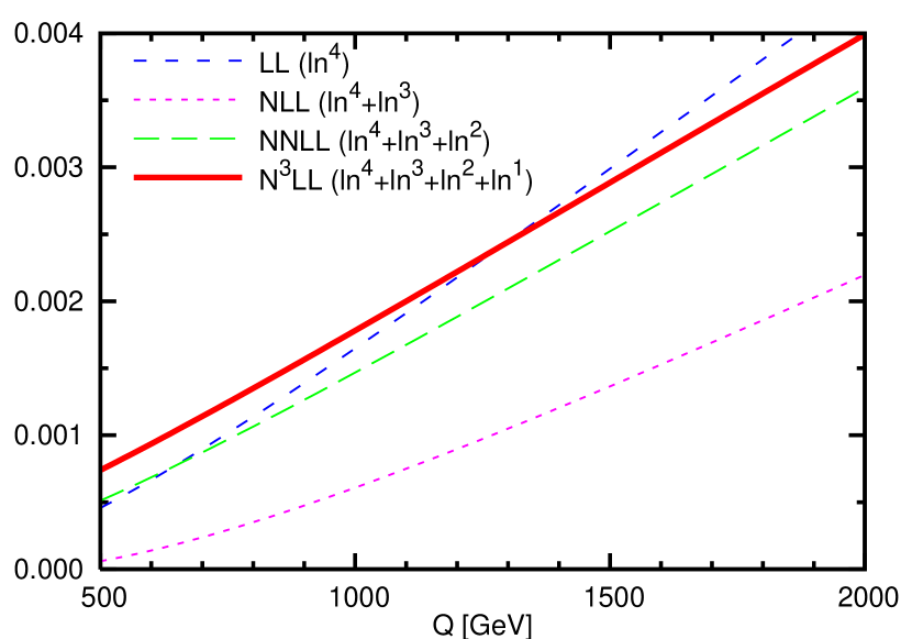
Figure 13: Two-loop contribution to the Abelian vector form factor $F_{2}$ in successive logarithmic approximations, using the values $M=80\,$GeV and $\alpha/(4\pi)=0.003$

The result presented here relies on the approximation that the Higgs mass is equal to the gauge boson mass, $M_{H}=M$. In order to investigate the dependence of the form factor on the Higgs mass, we have also calculated the Higgs contributions in the hypothetical case of a vanishing Higgs mass, $M_{H}=0$. Then equation (5) becomes

$$F_{2,\mathrm{Higgs}}^{M_{H}=0} =\left(\frac{\alpha}{4\pi}\right)^{2}\,\biggl{\{}-\frac{1}{24}\mathcal{L}^{3}+\frac{25}{48}\mathcal{L}^{2}-\biggl{(}\frac{3}{4}\sqrt{3}\,\mathrm{Cl}_{2}\!\left(\frac{\pi}{3}\right)$$

$$\qquad-\frac{1}{8}\sqrt{3}\pi-\frac{3}{16}\pi^{2}+\frac{25}{16}\biggr{)}\,\mathcal{L}\biggr{\}}+\mathcal{O}(\mathcal{L}^{0})\,.$$ (107)

Only the coefficient of the linear logarithm differs between equations (5) and (5). The coefficients of the cubic and quadratic logarithms are the same, they do not depend on the Higgs boson mass and have already been determined in the evolution equation approach Kuhn:2001hz ; Kuhn:2001hzE . By setting $M_{H}=0$, the coefficient of the linear logarithm of $F_{2,{C_{F}C_{A}+\mathrm{Higgs}}}$ in (5) numerically changes from 43 to 45, and the contribution of this term in (5) is shifted from $2.0$ to $2.1$. So the variation of the N³LL form factor between the two cases $M_{H}=M$ and $M_{H}=0$ is smaller than the total linear-logarithmic contribution by a factor of 3. On this basis we expect the deviation of the form factor with the true Higgs mass from our result to be comparable to the neglected non-logarithmic constant.

Altogether we estimate the accuracy of our form factor result to be of the order of the linear-logarithmic contribution, i.e. about half a per mil with respect to the Born result.

The result for the Abelian vector form factor presented in (5) has been combined in Jantzen:2005xi ; Jantzen:2005az with the reduced amplitude from equation (1) in order to obtain the four-fermion scattering amplitude in the spontaneously broken $SU(2)$ model in N³LL accuracy. In addition predictions for the electroweak model have been obtained by separating the infrared-divergent electromagnetic contributions (cf. appendix D) and by expanding in the mass difference between the $W$ and $Z$ bosons. For a discussion of this procedure and of the accuracy of the electroweak corrections we refer to Jantzen:2005xi ; Jantzen:2005az .

6 Summary

In the present paper we have discussed in detail the calculation of the two-loop corrections to the Abelian vector form factor in a spontaneously broken $SU(2)$ model. The result was obtained in N³LL accuracy and contains all logarithmically enhanced terms. It enables the derivation of electroweak corrections to four-fermion processes with an error of a few per mil to one percent, thus coping with the expected experimental accuracy at a future linear collider.

Appendix A Feynman rules

This appendix lists the Feynman rules of the vertices which are needed for the calculation of the form factor, as they follow from the Lagrangian of the spontaneously broken $SU(2)$ gauge model described in section 2.

The gauge boson fields of mass $M=M_{W}$ are $W^{a}_{\mu}$, $a=1,2,3$ (with Lorentz vector index $\mu$). To each $W^{a}$ corresponds a ghost field $c^{a}$ (and antighost $\bar{c}^{a}$) and a Goldstone boson $\phi^{a}$, one of the unphysical components of the Higgs doublet. In the Feynman–’t Hooft gauge used by us, there is $M_{c}=M_{\phi}=M_{W}$. The physical Higgs boson $H$ has the mass $M_{H}$. Finally, $\psi$ denotes a fermion (lepton or quark) doublet of Dirac spinors, and $g$ is the weak $SU(2)$ coupling.

Vertices involving four fields and vertices without a gauge boson do not appear in our present calculation and are omitted here.

Gauge boson coupling to fermions

$$\begin{tabular}[]{@{}c@{}}\raisebox{-8.61108pt}{\includegraphics{feynman-vertex-Wff.eps}}\end{tabular}=ig\gamma_{\mu}t^{a}$$

Gauge boson self-coupling

$$\begin{tabular}[]{@{}c@{}}\raisebox{-8.61108pt}{\includegraphics{feynman-vertex-WWW.eps}}\end{tabular}=\begin{cases}\begin{aligned} g\,f^{abc}\Bigl{[}\,&g_{\mu\nu}(k_{1}-k_{2})_{\rho}\\ +\,&g_{\nu\rho}(k_{2}-k_{3})_{\mu}\\ +\,&g_{\rho\mu}(k_{3}-k_{1})_{\nu}\Bigr{]}\end{aligned}\end{cases}$$

Gauge boson coupling to ghost fields

$$\begin{tabular}[]{@{}c@{}}\raisebox{-8.61108pt}{\includegraphics{feynman-vertex-Wcc.eps}}\end{tabular}=-g\,f^{abc}k_{\mu}$$

Gauge boson coupling to Higgs and Goldstone bosons

$$=igM\,g_{\mu\nu}\delta^{ab}$$

$$=\frac{g}{2}\delta^{ab}(k_{H}-k_{\phi})_{\mu}$$

$$=-\frac{g}{2}f^{abc}(k_{1}-k_{2})_{\mu}$$

In contrast to the other vertices above, which can be used in any $SU(N)$ gauge model, the couplings involving Higgs and Goldstone bosons are only valid for the spontaneously broken $SU(2)$ model.

Appendix B Expansion by regions

The asymptotic expansion of Feynman integrals in limits typical of Euclidean space is given by well-known prescriptions as a sum over certain subgraphs Chetyrkin:1988zz ; Chetyrkin:1988cu ; Gorishnii:1989dd ; Smirnov:1990rz ; Smirnov:1994tg . However, the Sudakov limit we are dealing with is typical of Minkowski space. Still for some special cases, similar graph-theoretical prescriptions were obtained Smirnov:1996ng ; Czarnecki:1996nr ; Smirnov:1997gx . In particular, as it was shown in Smirnov:1997gx , they can be applied to expand the planar two-loop diagram of figure 2a) in the Sudakov limit.

The bad news is that for other relevant diagrams, such as the non-planar and the Mercedes–Benz diagrams, graph-theoretical prescriptions are not available. The good news is that one can apply here (and for any other limit) the strategy of expansion by regions Beneke:1997zp ; Smirnov:1998vk ; Smirnov:1999bz ; Smirnov:2002pj which consists of the following prescriptions:

• Divide the space of the loop momenta into various regions and, in every region, expand the integrand in a Taylor series with respect to the parameters that are considered small there.

• Integrate the integrand, expanded in the appropriate way in every region, over the whole integration domain of the loop momenta.

• Set to zero any scaleless integral.

To apply this strategy to a given limit one should first understand, using various examples, which regions are relevant to it. In the Sudakov limit under consideration, these are the following regions, for a loop momentum $k$:

hard (h): $$k\sim Q\,,$$

1-collinear (1c): $$k_{+}\sim\frac{M^{2}}{Q}\,,\quad k_{-}\sim Q\,,\quad k_{\bot}\sim M\,,$$

2-collinear (2c): $$k_{+}\sim Q\,,\quad k_{-}\sim\frac{M^{2}}{Q}\,,\quad k_{\bot}\sim M\,,$$

soft (s): $$k\sim M\,,$$

ultrasoft (us): $$k\sim\frac{M^{2}}{Q}\,.$$

By $k\sim Q$ etc. we mean that any component of the vector $k$ is of order $Q$, and $k_{\pm}$, $k_{\bot}$ are the components of $k$ defined after equation (8). In other versions of the Sudakov limit, ultracollinear regions can also participate Smirnov:1999bz , but they are irrelevant to the present version.

So we obtain with this strategy the asymptotic expansion of our integrals as a sum of contributions generated by various regions. For brevity, we omit the word “generated” and speak about contributions of regions, although the integration in each contribution is performed over the whole space of the loop momenta.

In fact, this strategy is a generalization of the original strategy based on similar regions Sterman:1986aj ; Mueller:1979ih ; Collins:1989bt , where the cut-offs specifying the regions were not removed so that the integrations were bounded by the regions under consideration.

Appendix C Mellin–Barnes representation

The Mellin–Barnes representation is a powerful tool for solving two closely related problems: a) The calculation of Feynman integrals. b) The asymptotic expansion of Feynman integrals in various kinematical limits.

The basic identity of the Mellin–Barnes representation is the following (valid for $|\arg X-\arg Y|<\pi$):

$$\frac{1}{(X+Y)^{\lambda}}=\frac{1}{\Gamma(\lambda)}\int_{-i\infty}^{i\infty}\!\frac{\mathrm{d}z}{2\pi i}\,\Gamma(-z)\Gamma(\lambda+z)\,\frac{Y^{z}}{X^{\lambda+z}}\,.$$ (108)

It replaces a sum raised to any power by individual factors which are raised to powers depending on the Mellin–Barnes parameter $z$. This simplification of the structure is obtained at the cost of an additional integration. The integration contour in the Mellin–Barnes integrals runs from $-i\infty$ to $+i\infty$ and is chosen in such a way that poles from gamma functions of the form $\Gamma(\ldots+z)$ lie on the left hand side of the contour (“left poles”) and poles from gamma functions of the form $\Gamma(\ldots-z)$ lie on the right hand side of the contour (“right poles”). The contour cannot always be chosen as a straight line, especially if $\operatorname{Re}\lambda<0$.

If $|X|<|Y|$, the integration contour can be closed on the left hand side at $\operatorname{Re}z=-\infty$, and the integral is given by the sum over the residues at the left poles. This sum corresponds to the Taylor expansion of $1/(X+Y)^{\lambda}$ for $|X|<|Y|$. On the other hand, if $|X|>|Y|$, the contour can be closed on the right hand side at $\operatorname{Re}z=+\infty$, and the sum over the residues at the right poles corresponds to the Taylor expansion for $|X|>|Y|$. In the limiting case $|X|=|Y|$ the Mellin–Barnes integral is also convergent and is given by the sum of the residues on either the left or the right side of the contour – provided that these sums converge, which is often the case, especially when more than two gamma functions are present.

The first application of the Mellin–Barnes representation was, probably, in Usyukina:1975yg . The simplest possibility of using it is to transform massive propagators ($X=k^{2}$, $Y=-M^{2}$) into massless ones (see e.g. Boos:1990rg ; Davydychev:1990jt ; Davydychev:1990cq as early references). In general, one starts from Feynman, alpha or Schwinger parameters and uses the Mellin–Barnes representation to separate arbitrary terms raised to some powers in such a way that the resulting parametric integrals can be calculated in terms of gamma functions (see e.g. Greub:1996tg ; Greub:2000sy ; Asatryan:2001zw ; Bieri:2003ue ). In the context of dimensional regularization, when the explicit evaluation at general values of $d=4-2\varepsilon$ is hardly possible and one is oriented at calculating Feynman integrals in a Laurent expansion in $\varepsilon$, the systematic evaluation by Mellin–Barnes representations was initiated in Smirnov:1999gc ; Tausk:1999vh . An essential step of the evaluation procedure is the resolution of singularities in $\varepsilon$, with the goal to represent a given multiple Mellin–Barnes integral as a sum of integrals where the Laurent expansion of the integrands becomes possible. This is achieved by taking residues and shifting contours. Two different strategies for implementing this step were suggested in Smirnov:1999gc and Tausk:1999vh , respectively.

The identity (108) is valid for all powers $\lambda$. In fact, the crucial point is not the convergence of the integral in the basic identity (108), but the interchange of the order of integrations between the Mellin–Barnes integral and the (Feynman, alpha or Schwinger) parameter integrals. The necessary convergence of the parameter integrals restricts the real part of the Mellin–Barnes parameter $z$ to a specific range. If this range has a non-empty overlap with the interval $(-\operatorname{Re}\lambda,0)$, the integration contour over $z$ can be chosen as a straight line parallel to the imaginary axis within the allowed range on the real axis. One can find values for the power $\lambda$ and other parameters such that an allowed range for the real part of $z$ exists. The analytic continuation to the desired parameter values is then obtained by accounting for the residues which cross the fixed integration contour when the parameter values are smoothly changed Tausk:1999vh . Alternatively, the contour of the Mellin–Barnes integration can be deformed in such a way that it separates the poles of gamma functions with a “$+z$” dependence from the ones with a “$-z$” dependence even for the desired parameter values Smirnov:1999gc . Not only the gamma functions from the Mellin–Barnes representation (108), but also the ones introduced by the evaluation of the parameter integrals have to be considered here. As long as the prescription following equation (108) for the integration contour is respected, the convergence of the integrals is provided and all residues are accounted for on the correct side of the contour. This is still true if multiple Mellin–Barnes integrals are introduced by the iterated application of (108). Even when $\lambda$ is a non-positive integer and $\Gamma(\lambda)$ in the denominator gets singular, the right hand side of (108) is given by the limit where $\lambda$ approaches its actual value. In this case only a finite number of residues give non-vanishing contributions and reproduce the Binomial formula for $(X+Y)^{|\lambda|}$.

Often the Mellin–Barnes representation is used for asymptotic expansions (see e.g. Greub:1996tg ; Greub:2000sy ; Asatryan:2001zw ; Bieri:2003ue ; Smirnov:2002mg ; Friot:2005cu ). When the Mellin–Barnes integral contains the factor $t^{z}$ with some parameter $t$, the asymptotic expansion in the limit $t\to 0$ is given by picking up the residues on the right hand side of the integration contour. The asymptotic expansion in the limit $t\to\infty$ is given by the residues on the left hand side of the contour. By expanding $t^{z}$ in $z$ about the poles of the integrand, the explicit form of the asymptotic expansion in powers of $t$ and $\ln t$ with coefficients from the Laurent expansion of the Mellin–Barnes integrand can easily be obtained Friot:2005cu . In practice, however, the most adequate way to perform the asymptotic expansion depends on the specific problem. For the work presented in this paper we have applied the method of expansion by regions (appendix B) and used Mellin–Barnes representations in the purpose of asymptotic expansion as a cross-check. When calculating scalar integrals for general propagator powers $n_{i}$ as in section 3, the leading contributions can be obtained from the Mellin–Barnes representation by taking the residue at the first pole of each gamma function on the correct side of the integration contour. It turned out that in many cases the expressions obtained by the expansion of the loop integral within the expansion by regions method were simpler than the expressions extracted from the Mellin–Barnes representation of the full integral.

If the Mellin–Barnes representation is applied to the calculation of Feynman integrals (in particular, of individual contributions in an asymptotic expansion, as in the present work), when no large or small parameter $t$ is present as $t^{z}$ in the Mellin–Barnes integrals or when the full dependence on $t$ is desired, all residues on one side of the integration contour have to be considered and summed up. Some integrations in multiple Mellin–Barnes integrals can be performed explicitly by the application of identities based on the first Barnes lemma Barnes:1908 ,

$$\int_{-i\infty}^{i\infty}\!\frac{\mathrm{d}z}{2\pi i}\,\Gamma(\lambda_{1}+z)\Gamma(\lambda_{2}+z)\Gamma(\lambda_{3}-z)\Gamma(\lambda_{4}-z)\\ =\frac{\Gamma(\lambda_{1}+\lambda_{3})\Gamma(\lambda_{1}+\lambda_{4})\Gamma(\lambda_{2}+\lambda_{3})\Gamma(\lambda_{2}+\lambda_{4})}{\Gamma(\lambda_{1}+\lambda_{2}+\lambda_{3}+\lambda_{4})}\,,$$ (109)

or on the second Barnes lemma Barnes:1910 ,

$$\int_{-i\infty}^{i\infty}\!\frac{\mathrm{d}z}{2\pi i}\,\frac{\Gamma(\lambda_{1}+z)\Gamma(\lambda_{2}+z)\Gamma(\lambda_{3}+z)}{\Gamma(\lambda_{1}+\lambda_{2}+\lambda_{3}+\lambda_{4}+\lambda_{5}+z)}\\ \times\Gamma(\lambda_{4}-z)\Gamma(\lambda_{5}-z)\\ =\frac{\Gamma(\lambda_{1}+\lambda_{4})\Gamma(\lambda_{1}+\lambda_{5})\Gamma(\lambda_{2}+\lambda_{4})\Gamma(\lambda_{2}+\lambda_{5})}{\Gamma(\lambda_{1}+\lambda_{2}+\lambda_{4}+\lambda_{5})\Gamma(\lambda_{1}+\lambda_{3}+\lambda_{4}+\lambda_{5})}\\ \times\frac{\Gamma(\lambda_{3}+\lambda_{4})\Gamma(\lambda_{3}+\lambda_{5})}{\Gamma(\lambda_{2}+\lambda_{3}+\lambda_{4}+\lambda_{5})}$$ (110)

(see a collection of such formulae in Appendix D of Smirnov:2004ym ).

Mellin–Barnes integrals develop singularities when a left pole and a right pole glue together in one point for some limit, e.g. $\varepsilon\to 0$ from dimensional regularization. These singularitities are directly present in the formulae (109) and (110) of the first and second Barnes lemma. In more complicated cases, it is usually a good idea to first extract the potentially singular residues by shifting the integration contours Smirnov:1999gc or by an analytic continuation as described above and in Tausk:1999vh . Then the integrand may be expanded in the desired limits of its parameters. For an analytical result the residues on one side of the integration contour are summed up with the help of computer algebra programs, summation tables (see e.g. Smirnov:2004ym ) or algorithms like Moch:2001zr ; Weinzierl:2004bn .

Characteristic examples of recent sophisticated calculations based on the technique of Mellin–Barnes representations can be found in Smirnov:2003vi ; Bern:2005iz . These results were crucial to check (in Bern:2005iz ) cross order relations in $N=4$ supersymmetric Yang–Mills theory conjectured in Anastasiou:2003kj . Very recent results on checking the iteration structure in this theory with the help of Mellin–Barnes representations have been obtained in Cachazo:2006mq ; Cachazo:2006tj ; Bern:2006vw .

Also recently algorithms for the automatic evaluation of Mellin–Barnes integrals have been formulated Anastasiou:2005cb ; Czakon:2005rk . These rely on the strategy of Tausk:1999vh for the analytic continuation in the parameter $\varepsilon$. The algorithms provide a basis for the analytic evaluation, and at least they can be applied, in their present form, to the numerical evaluation. The algorithm of Czakon:2005rk is already implemented in Mathematica and would have been applied by us at least for numerical checks if it had existed early enough.

Appendix D Contributions in a theory with a mass gap

The separation of the infrared-divergent electromagnetic contributions as described in Feucht:2004rp requires the two-loop corrections in the combined $SU(2)\times U(1)$ or $U(1)\times U(1)$ theory with massive and massless gauge bosons. In addition to the results presented in the sections 3 and 4 of this paper, two-loop vertex and self-energy corrections with one massive $SU(2)$ or $U(1)$ gauge boson and one massless $U(1)$ gauge boson are needed.

As we regard an $SU(2)\times U(1)$ model without mixing between the two gauge groups (see Jantzen:2005xi ; Jantzen:2005az for a discussion of this aspect), only the Abelian vertex and self-energy diagrams (figures 2 and 11) contribute. After replacing one of the two massive $SU(2)$ gauge bosons in these diagrams by a massless $U(1)$ gauge boson, we obtain the results listed in the following paragraphs.

The planar vertex correction of the diagram in figure 2a) with line 5 (cf. figure 4) massless is

$$F_{\mathrm{v},\mathrm{LA}}^{M_{5}=0} =C_{F}\,\frac{\alpha\alpha^{\prime}}{(4\pi)^{2}}\left(\frac{\mu^{2}}{M^{2}}\right)^{2\varepsilon}S_{\varepsilon}^{2}\,\Biggl{\{}-\frac{2}{\varepsilon^{3}}$$

$$\quad+\frac{1}{\varepsilon^{2}}\left[2\mathcal{L}^{2}-4\mathcal{L}+\frac{4}{3}\pi^{2}+\frac{9}{2}\right]+\frac{1}{\varepsilon}\,\biggl{[}-\frac{4}{3}\mathcal{L}^{3}$$

$$\qquad+4\mathcal{L}^{2}+\left(\frac{2}{3}\pi^{2}-17\right)\mathcal{L}+12\zeta_{3}-\frac{7}{3}\pi^{2}+\frac{85}{4}\biggr{]}$$

$$\quad+\frac{2}{3}\mathcal{L}^{4}-\frac{8}{3}\mathcal{L}^{3}+\left(\frac{\pi^{2}}{3}+17\right)\mathcal{L}^{2}$$

$$\quad+\left(-36\zeta_{3}+\frac{2}{3}\pi^{2}-\frac{101}{2}\right)\mathcal{L}+\frac{107}{90}\pi^{4}+\frac{184}{3}\zeta_{3}$$

$$\quad-\frac{59}{12}\pi^{2}+\frac{599}{8}\Biggr{\}}+\mathcal{O}(\varepsilon)+\mathcal{O}\!\left(\frac{M^{2}}{Q^{2}}\right),$$ (111)

where $\alpha$ and $\alpha^{\prime}$ are the couplings of the $SU(2)$ and $U(1)$ gauge groups, respectively, and $\mathcal{L}=\ln(Q^{2}/M^{2})$. The $1/\varepsilon^{3}$ pole is due to the infrared divergence. The same diagram with line 6 massless yields the contribution

$$F_{\mathrm{v},\mathrm{LA}}^{M_{6}=0} =C_{F}\,\frac{\alpha\alpha^{\prime}}{(4\pi)^{2}}\left(\frac{\mu^{2}}{M^{2}}\right)^{2\varepsilon}S_{\varepsilon}^{2}\,\Biggl{\{}\frac{1}{2\varepsilon^{2}}$$

$$\qquad+\frac{1}{\varepsilon}\left[-\mathcal{L}^{2}+3\mathcal{L}-\frac{2}{3}\pi^{2}-\frac{11}{4}\right]+\frac{1}{6}\mathcal{L}^{4}$$

$$\qquad+\left(\frac{2}{3}\pi^{2}-1\right)\mathcal{L}^{2}+\left(-24\zeta_{3}-\pi^{2}+\frac{11}{2}\right)\mathcal{L}$$

$$\qquad+\frac{13}{45}\pi^{4}+46\zeta_{3}+\frac{13}{12}\pi^{2}-\frac{41}{8}\Biggr{\}}$$

$$\quad+\mathcal{O}(\varepsilon)+\mathcal{O}\!\left(\frac{M^{2}}{Q^{2}}\right).$$ (112)

Note that only the linear logarithm and the non-logarithmic constant at order $\varepsilon^{0}$ of this result differ from the case (3.3) with two massive gauge bosons (and, of course, the different prefactor $C_{F}\,\alpha\alpha^{\prime}$ instead of $C_{F}^{2}\,\alpha^{2}$).

When either of the two gauge bosons in the non-planar vertex diagram of figure 2b) is massless (cf. figure 5 for the line numbering), the contribution is

$$F_{\mathrm{v},\mathrm{NP}}^{M_{5}=0} =F_{\mathrm{v},\mathrm{NP}}^{M_{6}=0}=C_{F}\,\frac{\alpha\alpha^{\prime}}{(4\pi)^{2}}\left(\frac{\mu^{2}}{M^{2}}\right)^{2\varepsilon}S_{\varepsilon}^{2}\,\Biggl{\{}$$

$$\qquad\frac{1}{\varepsilon}\left[-\frac{2}{3}\mathcal{L}^{3}+4\mathcal{L}^{2}-12\mathcal{L}-12\zeta_{3}+\pi^{2}+14\right]$$

$$\qquad+\frac{1}{2}\mathcal{L}^{4}-4\mathcal{L}^{3}+\left(-\frac{5}{3}\pi^{2}+22\right)\mathcal{L}^{2}$$

$$\qquad+\left(56\zeta_{3}+\frac{11}{3}\pi^{2}-68\right)\mathcal{L}-\frac{67}{90}\pi^{4}-90\zeta_{3}$$

$$\qquad-4\pi^{2}+96\Biggr{\}}+\mathcal{O}(\varepsilon)+\mathcal{O}\!\left(\frac{M^{2}}{Q^{2}}\right)\,.$$ (113)

The Mercedes–Benz graph in figure 2c) gives the contribution

$$F_{\mathrm{v},\mathrm{BE}}^{M_{3}=0} =C_{F}\,\frac{\alpha\alpha^{\prime}}{(4\pi)^{2}}\left(\frac{\mu^{2}}{M^{2}}\right)^{2\varepsilon}S_{\varepsilon}^{2}\,\Biggl{\{}\frac{1}{2\varepsilon^{2}}$$

$$\qquad+\frac{1}{\varepsilon}\,\biggl{[}-\mathcal{L}^{2}+\left(-\frac{2}{3}\pi^{2}+7\right)\mathcal{L}+4\zeta_{3}+\frac{\pi^{2}}{3}$$

$$\qquad\qquad-\frac{53}{4}\biggr{]}+\mathcal{L}^{3}+\left(\frac{2}{3}\pi^{2}-9\right)\mathcal{L}^{2}$$

$$\qquad+\left(-4\zeta_{3}-3\pi^{2}+\frac{89}{2}\right)\mathcal{L}-\frac{13}{90}\pi^{4}+16\zeta_{3}$$

$$\qquad+\frac{79}{12}\pi^{2}-\frac{655}{8}\Biggr{\}}+\mathcal{O}(\varepsilon)+\mathcal{O}\!\left(\frac{M^{2}}{Q^{2}}\right),$$ (114)

when line 3 (cf. figure 6) is massless, and

$$F_{\mathrm{v},\mathrm{BE}}^{M_{4}=0} =C_{F}\,\frac{\alpha\alpha^{\prime}}{(4\pi)^{2}}\left(\frac{\mu^{2}}{M^{2}}\right)^{2\varepsilon}S_{\varepsilon}^{2}\,\Biggl{\{}-\frac{2}{\varepsilon^{3}}+\frac{1}{\varepsilon^{2}}\left[2\mathcal{L}-\frac{5}{2}\right]$$

$$\qquad+\frac{1}{\varepsilon}\left[-2\mathcal{L}^{2}+7\mathcal{L}-\frac{\pi^{2}}{3}-\frac{53}{4}\right]+\frac{4}{3}\mathcal{L}^{3}$$

$$\qquad+\left(\frac{\pi^{2}}{3}-9\right)\mathcal{L}^{2}+\left(8\zeta_{3}-\frac{7}{3}\pi^{2}+\frac{73}{2}\right)\mathcal{L}$$

$$\qquad+\frac{11}{45}\pi^{4}-\frac{32}{3}\zeta_{3}+\frac{17}{4}\pi^{2}-\frac{479}{8}\Biggr{\}}$$

$$\quad+\mathcal{O}(\varepsilon)+\mathcal{O}\!\left(\frac{M^{2}}{Q^{2}}\right),$$ (115)

when line 4 is massless.

The vertex correction with fermion self-energy of the diagram in figure 2d) yields

$$F_{\mathrm{v},\mathrm{fc}}^{M_{3}=0} =C_{F}\,\frac{\alpha\alpha^{\prime}}{(4\pi)^{2}}\left(\frac{\mu^{2}}{M^{2}}\right)^{2\varepsilon}S_{\varepsilon}^{2}\,\Biggl{\{}\frac{2}{\varepsilon^{3}}+\frac{1}{\varepsilon^{2}}\left[-2\mathcal{L}+\frac{5}{2}\right]$$

$$\qquad+\frac{1}{\varepsilon}\left[2\mathcal{L}^{2}-7\mathcal{L}+\frac{\pi^{2}}{3}+\frac{53}{4}\right]-\frac{4}{3}\mathcal{L}^{3}+7\mathcal{L}^{2}$$

$$\qquad+\left(\frac{\pi^{2}}{3}-\frac{53}{2}\right)\mathcal{L}-\frac{40}{3}\zeta_{3}-\frac{13}{12}\pi^{2}+\frac{355}{8}\Biggr{\}}$$

$$\quad+\mathcal{O}(\varepsilon)+\mathcal{O}\!\left(\frac{M^{2}}{Q^{2}}\right),$$ (116)

with line 3 (cf. figure 7) massless and

$$F_{\mathrm{v},\mathrm{fc}}^{M_{5}=0} =C_{F}\,\frac{\alpha\alpha^{\prime}}{(4\pi)^{2}}\left(\frac{\mu^{2}}{M^{2}}\right)^{2\varepsilon}S_{\varepsilon}^{2}\,\Biggl{\{}-\frac{1}{2\varepsilon^{2}}$$

$$\qquad+\frac{1}{\varepsilon}\left[\mathcal{L}^{2}-3\mathcal{L}+\frac{2}{3}\pi^{2}+\frac{13}{4}\right]-\mathcal{L}^{3}+5\mathcal{L}^{2}$$

$$\qquad-\frac{33}{2}\mathcal{L}-4\zeta_{3}+\frac{\pi^{2}}{12}+\frac{163}{8}\Biggr{\}}$$

$$\quad+\mathcal{O}(\varepsilon)+\mathcal{O}\!\left(\frac{M^{2}}{Q^{2}}\right),$$ (117)

with line 5 massless. The only difference of (D) with respect to the purely massive result (3.6) is in the non-logarithmic constant at order $\varepsilon^{0}$.

The self-energy diagram in figure 11a) contributes

$$\Sigma_{\mathrm{T1}}^{M_{2}=0}=\Sigma_{\mathrm{T1}}^{M_{3}=0} =C_{F}\,\frac{\alpha\alpha^{\prime}}{(4\pi)^{2}}\left(\frac{\mu^{2}}{M^{2}}\right)^{2\varepsilon}S_{\varepsilon}^{2}\left(\frac{1}{2\varepsilon}-\frac{3}{4}\right)$$

$$\qquad+\mathcal{O}(\varepsilon)\,,$$ (118)

when either of its two gauge bosons is massless. The two contributions of the self-energy diagram in figure 11b) are

$$\Sigma_{\mathrm{T2}}^{M_{2}=0} =C_{F}\,\frac{\alpha\alpha^{\prime}}{(4\pi)^{2}}\left(\frac{\mu^{2}}{M^{2}}\right)^{2\varepsilon}S_{\varepsilon}^{2}\left(-\frac{1}{2\varepsilon^{2}}+\frac{3}{4\varepsilon}-\frac{\pi^{2}}{4}-\frac{1}{8}\right)$$

$$\qquad+\mathcal{O}(\varepsilon)\,,$$ (119)

with the gauge boson in the outer loop massless, and

$$\Sigma_{\mathrm{T2}}^{M_{4}=0} =C_{F}\,\frac{\alpha\alpha^{\prime}}{(4\pi)^{2}}\left(\frac{\mu^{2}}{M^{2}}\right)^{2\varepsilon}S_{\varepsilon}^{2}\left(\frac{1}{2\varepsilon^{2}}-\frac{1}{4\varepsilon}+\frac{\pi^{2}}{4}-\frac{1}{8}\right)$$

$$\qquad+\mathcal{O}(\varepsilon)\,,$$ (120)

with the gauge boson in the inner loop massless. Note that (D) differs from the purely massive result (4.1) only at order $\varepsilon^{0}$.

The self-energy diagram in figure 11c) has no corresponding contribution with one massive and one massless gauge boson, because these integrals vanish in dimensional regularization.

According to (69), the product of the massless one-loop vertex correction $F_{\mathrm{v},1}^{M=0}$ and the (massive) one-loop self-energy correction $\Sigma_{1}$ (4.1) is needed as well. The missing piece is well known:

$$F_{\mathrm{v},1}^{M=0}=\frac{\alpha^{\prime}}{4\pi}\left(\frac{\mu^{2}}{Q^{2}}\right)^{\varepsilon}S_{\varepsilon}\,\Biggl{\{}-\frac{2}{\varepsilon^{2}}-\frac{3}{\varepsilon}+\frac{\pi^{2}}{6}-8\\ +\varepsilon\left(\frac{14}{3}\zeta_{3}+\frac{\pi^{2}}{4}-16\right)\Biggr{\}}+\mathcal{O}(\varepsilon^{2})\,.$$ (121)

The prefactor has to be expanded as

$$\left(\frac{\mu^{2}}{Q^{2}}\right)^{\varepsilon}=\left(\frac{\mu^{2}}{M^{2}}\right)^{\varepsilon}\left(1-\varepsilon\mathcal{L}+\frac{\varepsilon^{2}}{2}\mathcal{L}^{2}-\frac{\varepsilon^{3}}{6}\mathcal{L}^{3}\right)+\mathcal{O}(\varepsilon^{4})$$

in order to match the prefactor of the other contributions.

The contributions to the $SU(2)\times U(1)$ form factor with one massive and one massless gauge boson may now be added together in analogy with (5):

$$F_{2,\alpha\alpha^{\prime}} =F_{\mathrm{v},\mathrm{LA}}^{M_{5}=0}+F_{\mathrm{v},\mathrm{LA}}^{M_{6}=0}+F_{\mathrm{v},\mathrm{NP}}^{M_{5}=0}+F_{\mathrm{v},\mathrm{NP}}^{M_{6}=0}$$

$$\qquad+2\,F_{\mathrm{v},\mathrm{BE}}^{M_{3}=0}+2\,F_{\mathrm{v},\mathrm{BE}}^{M_{4}=0}+2\,F_{\mathrm{v},\mathrm{fc}}^{M_{3}=0}+2\,F_{\mathrm{v},\mathrm{fc}}^{M_{5}=0}$$

$$\qquad+\Sigma_{\mathrm{T1}}^{M_{2}=0}+\Sigma_{\mathrm{T1}}^{M_{3}=0}+\Sigma_{\mathrm{T2}}^{M_{2}=0}+\Sigma_{\mathrm{T2}}^{M_{4}=0}$$

$$\qquad+F_{\mathrm{v},1}^{M=0}\Sigma_{1}$$

$$=C_{F}\,\frac{\alpha\alpha^{\prime}}{(4\pi)^{2}}\left(\frac{\mu^{2}}{M^{2}}\right)^{2\varepsilon}S_{\varepsilon}^{2}\,\Biggl{\{}$$

$$\qquad\frac{1}{\varepsilon^{2}}\left[2\mathcal{L}^{2}-6\mathcal{L}+\frac{4}{3}\pi^{2}+7\right]+\frac{1}{\varepsilon}\,\biggl{[}-\frac{8}{3}\mathcal{L}^{3}+12\mathcal{L}^{2}$$

$$\qquad\qquad+\left(-\frac{2}{3}\pi^{2}-32\right)\mathcal{L}-4\zeta_{3}+\pi^{2}+34\biggr{]}$$

$$\qquad+\frac{11}{6}\mathcal{L}^{4}-11\mathcal{L}^{3}+\left(-\frac{\pi^{2}}{3}+49\right)\mathcal{L}^{2}$$

$$\qquad+\Bigl{(}60\zeta_{3}-3\pi^{2}-111\Bigr{)}\,\mathcal{L}+\frac{17}{90}\pi^{4}-102\zeta_{3}$$

$$\qquad+\frac{47}{6}\pi^{2}+117\Biggr{\}}+\mathcal{O}(\varepsilon)+\mathcal{O}\!\left(\frac{M^{2}}{Q^{2}}\right).$$ (122)

The infrared-convergent two-loop interference term of equation (6) in Feucht:2004rp results from (D) after subtraction of the massive times the massless one-loop form factor: $F_{2,\alpha\alpha^{\prime}}-(F_{\mathrm{v},1}+\Sigma_{1})\cdot F_{\mathrm{v},1}^{M=0}$.

References

• (1) V.V. Sudakov, Sov. Phys. JETP 3, 65 (1956)
• (2) R. Jackiw, Ann. Phys. 48, 292 (1968)
• (3) M. Kuroda, G. Moultaka, D. Schildknecht, Nucl. Phys. B 350, 25 (1991)
• (4) G. Degrassi, A. Sirlin, Phys. Rev. D 46, 3104 (1992)
• (5) M. Beccaria, G. Montagna, F. Piccinini, F.M. Renard, C. Verzegnassi, Phys. Rev. D 58, 093014 (1998)
• (6) P. Ciafaloni, D. Comelli, Phys. Lett. B 446, 278 (1999)
• (7) J.H. Kühn, A.A. Penin, TTP/99-28, hep-ph/9906545, 1999
• (8) V.S. Fadin, L.N. Lipatov, A.D. Martin, M. Melles, Phys. Rev. D 61, 094002 (2000)
• (9) J.H. Kühn, A.A. Penin, V.A. Smirnov, Eur. Phys. J. C 17, 97 (2000)
• (10) J.H. Kühn, A.A. Penin, V.A. Smirnov, Nucl. Phys. B (Proc. Suppl.) 89, 94 (2000)
• (11) J.H. Kühn, S. Moch, A.A. Penin, V.A. Smirnov, Nucl. Phys. B 616, 286 (2001)
• (12) J.H. Kühn, S. Moch, A.A. Penin, V.A. Smirnov, Nucl. Phys. B 648, 455(E) (2003)
• (13) M. Beccaria, P. Ciafaloni, D. Comelli, F.M. Renard, C. Verzegnassi, Phys. Rev. D 61, 011301 (2000)
• (14) M. Beccaria, P. Ciafaloni, D. Comelli, F.M. Renard, C. Verzegnassi, Phys. Rev. D 61, 073005 (2000)
• (15) M. Beccaria, F.M. Renard, C. Verzegnassi, Phys. Rev. D 63, 053013 (2001)
• (16) M. Beccaria, F.M. Renard, C. Verzegnassi, Phys. Rev. D 64, 073008 (2001)
• (17) A. Denner, S. Pozzorini, Eur. Phys. J. C 18, 461 (2001)
• (18) A. Denner, S. Pozzorini, Eur. Phys. J. C 21, 63 (2001)
• (19) M. Melles, Phys. Rev. D 64, 014011 (2001)
• (20) M. Hori, H. Kawamura, J. Kodaira, Phys. Lett. B 491, 275 (2000)
• (21) W. Beenakker, A. Werthenbach, Nucl. Phys. B 630, 3 (2002)
• (22) B. Feucht, J.H. Kühn, S. Moch, Phys. Lett. B 561, 111 (2003)
• (23) A. Denner, M. Melles, S. Pozzorini, Nucl. Phys. B 662, 299 (2003)
• (24) M. Beccaria, F.M. Renard, C. Verzegnassi, Nucl. Phys. B 663, 394 (2003)
• (25) M. Beccaria, M. Melles, F.M. Renard, S. Trimarchi, C. Verzegnassi, Int. J. Mod. Phys. A 18, 5069 (2003)
• (26) S. Pozzorini, Nucl. Phys. B 692, 135 (2004)
• (27) B. Feucht, J.H. Kühn, A.A. Penin, V.A. Smirnov, Phys. Rev. Lett. 93, 101802 (2004)
• (28) J.H. Kühn, A. Kulesza, S. Pozzorini, M. Schulze, Phys. Lett. B 609, 277 (2005)
• (29) J.H. Kühn, A. Kulesza, S. Pozzorini, M. Schulze, Nucl. Phys. B 727, 368 (2005)
• (30) J.H. Kühn, A. Kulesza, S. Pozzorini, M. Schulze, JHEP 03, 059 (2006)
• (31) E. Accomando, A. Denner, A. Kaiser, Nucl. Phys. B 706, 325 (2005)
• (32) A. Denner, S. Pozzorini, Nucl. Phys. B 717, 48 (2005)
• (33) B. Jantzen, J.H. Kühn, A.A. Penin, V.A. Smirnov, Phys. Rev. D 72, 051301(R) (2005)
• (34) B. Jantzen, J.H. Kühn, A.A. Penin, V.A. Smirnov, Nucl. Phys. B 731, 188 (2005)
• (35) J.M. Cornwall, G. Tiktopoulos, Phys. Rev. Lett. 35, 338 (1975)
• (36) J.M. Cornwall, G. Tiktopoulos, Phys. Rev. D 13, 3370 (1976)
• (37) J. Frenkel, J.C. Taylor, Nucl. Phys. B 116, 185 (1976)
• (38) D. Amati, R. Petronzio, G. Veneziano, Nucl. Phys. B 146, 29 (1978)
• (39) A.H. Mueller, Phys. Rev. D 20, 2037 (1979)
• (40) J.C. Collins, Phys. Rev. D 22, 1478 (1980)
• (41) J.C. Collins, in Perturbative quantum chromodynamics, edited by A.H. Mueller (World Scientific, 1989), p. 573, hep-ph/0312336
• (42) A. Sen, Phys. Rev. D 24, 3281 (1981)
• (43) A. Sen, Phys. Rev. D 28, 860 (1983)
• (44) G. Sterman, Nucl. Phys. B 281, 310 (1987)
• (45) J. Botts, G. Sterman, Nucl. Phys. B 325, 62 (1989)
• (46) W. Bernreuther, R. Bonciani, T. Gehrmann, R. Heinesch, T. Leineweber, P. Mastrolia, E. Remiddi, Nucl. Phys. B 706, 245 (2005)
• (47) G. ’t Hooft, M.J.G. Veltman, Nucl. Phys. B 44, 189 (1972)
• (48) J.A.M. Vermaseren, math-ph/0010025, 2000
• (49) Wolfram Research, Inc., Mathematica, Version 4.2, 2002
• (50) F.V. Tkachov, Phys. Lett. B 100, 65 (1981)
• (51) K.G. Chetyrkin, F.V. Tkachov, Nucl. Phys. B 192, 159 (1981)
• (52) V.A. Smirnov, Applied Asymptotic Expansions in Momenta and Masses, Springer Tracts in Modern Physics 177 (Springer, Berlin, 2002)
• (53) G. Kramer, B. Lampe, Z. Phys. C 34, 497 (1987)
• (54) G. Kramer, B. Lampe, Z. Phys. C 42, 504(E) (1989)
• (55) T. Matsuura, S.C. van der Marck, W.L. van Neerven, Nucl. Phys. B 319, 570 (1989)
• (56) V.A. Smirnov, Evaluating Feynman Integrals, Springer Tracts in Modern Physics 211 (Springer, Berlin, 2004)
• (57) V.A. Smirnov, Phys. Lett. B 404, 101 (1997)
• (58) V.A. Smirnov, E.R. Rakhmetov, Theor. Math. Phys. 120, 870 (1999)
• (59) V.A. Smirnov, Phys. Lett. B 524, 129 (2002)
• (60) J. Fleischer, A.V. Kotikov, O.L. Veretin, Nucl. Phys. B 547, 343 (1999)
• (61) J.A.M. Vermaseren, Int. J. Mod. Phys. A 14, 2037 (1999)
• (62) U. Aglietti, R. Bonciani, Nucl. Phys. B 698, 277 (2004)
• (63) G. Passarino, M.J.G. Veltman, Nucl. Phys. B 160, 151 (1979)
• (64) R.J. Gonsalves, Phys. Rev. D 28, 1542 (1983)
• (65) S. Moch, P. Uwer, S. Weinzierl, J. Math. Phys. 43, 3363 (2002)
• (66) S. Weinzierl, J. Math. Phys. 45, 2656 (2004)
• (67) M.Yu. Kalmykov, O. Veretin, Phys. Lett. B 483, 315 (2000)
• (68) H.R.P. Ferguson, D.H. Bailey, RNR Technical Report RNR-91-032, NASA Ames Research Center, 1991
• (69) D.H. Bailey, J.M. Borwein, R. Girgensohn, Experimental Mathematics 3, 17 (1994)
• (70) H.R.P. Ferguson, D.H. Bailey, S. Arno, Mathematics of Computation 68, 351 (1999)
• (71) O. Veretin (private communication)
• (72) D.H. Bailey, RNR Technical Report RNR-90-022, NASA Ames Research Center, 1990
• (73) D.H. Bailey, RNR Technical Report RNR-91-025, NASA Ames Research Center, 1991
• (74) D.J. Gross, F. Wilczek, Phys. Rev. Lett. 30, 1343 (1973)
• (75) H.D. Politzer, Phys. Rev. Lett. 30, 1346 (1973)
• (76) K.G. Chetyrkin, Theor. Math. Phys. 75, 346 (1988)
• (77) K.G. Chetyrkin, Theor. Math. Phys. 76, 809 (1988)
• (78) S.G. Gorishny, Nucl. Phys. B 319, 633 (1989)
• (79) V.A. Smirnov, Commun. Math. Phys. 134, 109 (1990)
• (80) V.A. Smirnov, Mod. Phys. Lett. A 10, 1485 (1995)
• (81) V.A. Smirnov, Phys. Lett. B 394, 205 (1997)
• (82) A. Czarnecki, V.A. Smirnov, Phys. Lett. B 394, 211 (1997)
• (83) M. Beneke, V.A. Smirnov, Nucl. Phys. B 522, 321 (1998)
• (84) V.A. Smirnov, Phys. Lett. B 465, 226 (1999)
• (85) N.I. Ussyukina, Theor. Math. Phys. 22, 210 (1975)
• (86) E.E. Boos, A.I. Davydychev, Theor. Math. Phys. 89, 1052 (1991)
• (87) A.I. Davydychev, J. Math. Phys. 32, 1052 (1991)
• (88) A.I. Davydychev, J. Math. Phys. 33, 358 (1992)
• (89) C. Greub, T. Hurth, D. Wyler, Phys. Rev. D 54, 3350 (1996)
• (90) C. Greub, P. Liniger, Phys. Rev. D 63, 054025 (2001)
• (91) H.H. Asatryan, H.M. Asatrian, C. Greub, M. Walker, Phys. Rev. D 65, 074004 (2002)
• (92) K. Bieri, C. Greub, M. Steinhauser, Phys. Rev. D 67, 114019 (2003)
• (93) V.A. Smirnov, Phys. Lett. B 460, 397 (1999)
• (94) J.B. Tausk, Phys. Lett. B 469, 225 (1999)
• (95) V.A. Smirnov, Phys. Lett. B 547, 239 (2002)
• (96) S. Friot, D. Greynat, E. de Rafael, Phys. Lett. B 628, 73 (2005)
• (97) E.W. Barnes, Proc. London Math. Soc. (2) 6, 141 (1908)
• (98) E.W. Barnes, Quart. J. of Pure and Applied Math. 41, 136 (1910)
• (99) V.A. Smirnov, Phys. Lett. B 567, 193 (2003)
• (100) Z. Bern, L.J. Dixon, V.A. Smirnov, Phys. Rev. D 72, 085001 (2005)
• (101) C. Anastasiou, Z. Bern, L.J. Dixon, D.A. Kosower, Phys. Rev. Lett. 91, 251602 (2003)
• (102) F. Cachazo, M. Spradlin, A. Volovich, hep-th/0601031, 2006
• (103) F. Cachazo, M. Spradlin, A. Volovich, hep-th/0602228, 2006
• (104) Z. Bern, M. Czakon, D.A. Kosower, R. Roiban, V.A. Smirnov, hep-th/0604074, 2006
• (105) C. Anastasiou, A. Daleo, hep-ph/0511176, 2005
• (106) M. Czakon, hep-ph/0511200, 2005