Numerical Approach to Multi Dimensional Phase Transitions

Abstract

We present an algorithm to analyze numerically the bounce solution of first-order phase transitions. Our approach is well suited to treat phase transitions with several fields. The algorithm consists of two parts. In the first part the bounce solution without damping is determined, in which case energy is conserved. In the second part the continuation to the physically relevant case with damping is performed. The presented approach is numerically stable and easily implemented.

I Introduction

The problem of calculating properties of a first-order phase transition from a false vacuum to an energetically lower vacuum appears in different contexts of physics, as for example condensed matter physics Langer:1967ax ; Langer:1969bc , particle physics cole1 ; cole2 , and cosmology Affleck:1980ac ; Linde:1977mm ; Linde:1981zj . In a cosmological context, one of the interesting features of a first-order phase transition is that it can proceed by bubble nucleation. The subsequently expanding bubbles can be utilized as a source that drives the hot plasma in the early Universe out of equilibrium. This is in turn one of the Sakharov conditions, the requirements for a viable baryogenesis mechanism. Employing the electroweak phase transition, the corresponding baryogenesis mechanism was suggested in Ref. Kuzmin:1985mm and named electroweak baryogenesis. Even though this scenario of the generation of the baryon asymmetry of the Universe (BAU) is excluded in the Standard Model (SM) because of a lack of CP violation and the cross-over nature of the phase transition, this possibility is still open in the Minimal Supersymmetric Standard Model (MSSM) Carena:2002ss ; Carena:2000id ; Konstandin:2005cd . An essential input parameter of the determination of the produced BAU is the wall shape of the expanding bubbles. While in the SM the phase transition is described by a single vev of the Higgs field $v$, there are already two dynamical fields during the phase transition in the MSSM, namely two vevs, $v_{1}$ and $v_{2}$, or equivalently, $v=\sqrt{v_{1}^{2}+v_{2}^{2}}$ and $\tan(\beta)=v_{2}/v_{1}$. Notice that the initial value of $\beta$ cannot be inferred without studying the dynamics of the phase transition, since $v$ vanishes in the symmetric phase. This is especially important, because some CP violating sources are proportional to the change of $\beta$ during the phase transition.

Examining extensions of the MSSM, one has eventually to deal with more than two scalar fields. This is the case e.g. in the MSSM extended by an additional singlet Davies:1996qn ; Bastero-Gil:2000bw ; Menon:2004wv , which provides the interesting feature of transitional CP violation Huber:2000mg . Further examples are provided by models that equip this singlet with a $U(1)^{\prime}$ gauge symmetry Kang:2004pp or by the SM with two Higgs doublets Cline:1995dg ; Cline:1996mg .

The theoretical basis for the determination of the tunneling rates in particle physics and the explicit solution for one scalar field was given in cole1 ; cole2 . However to calculate the properties in the case of several scalar fields is analytically not accessible, and even numerically a non-trivial task. We present a numerical solution to this problem.

II The Problem

Before the numerical treatment of the multi field case is discussed, we will briefly review the results of cole1 ; cole2 and clarify our notation. Given the Lagrangian

$${\cal L}=\frac{1}{2}\partial_{\mu}\phi\partial^{\mu}\phi-V(\phi),$$ (1)

the transition probability per unit time and unit volume from a false vacuum to an energetically lower vacuum is, in the semi-classical approximation, given by

$$\Gamma=\frac{S[\bar{\phi}]^{2}}{4\pi^{2}\hbar^{2}}\,\exp({-S[\bar{\phi}]/\hbar})\left|\frac{\det^{\prime}[-\partial^{2}+V^{{}^{\prime\prime}}(\bar{\phi})]}{\det[-\partial^{2}+V^{{}^{\prime\prime}}(0)]}\right|^{-\frac{1}{2}}\times(1+O(\hbar)).$$ (2)

The primed determinant indicates that the zero-modes, corresponding to translation invariance, have been omitted, leading to the factor $S[\bar{\phi}]^{2}$ in the formula. The function $\bar{\phi}$ is the classical Euclidean solution of the equations of motion derived from the Lagrangian in Eq. (1) with inverted potential and the boundary conditions

$$\lim_{\tau\to\infty}\bar{\phi}(\tau,\vec{x})=\phi_{-},$$ (3)

where $\phi_{-}$ denotes the false vacuum and

$$\partial_{\tau}\bar{\phi}(0,\vec{x})=0.$$ (4)

In addition the solution should be non-trivial in the sense that $\bar{\phi}(0,\vec{x})=\phi_{b}$ is close to the new vacuum. The corresponding solution is usually called bounce configuration and a typical potential is illustrated in Fig. 1.

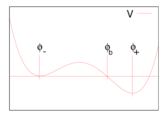
Figure 1: The potential for a theory with a false vacuum.

The present work aims at determining numerically the bounce configuration $\bar{\phi}$ in theories with several scalar fields. Thus, the parameters that are inferred about the phase transition rely on the semi-classical expansion in Eq. (2), which can break down, e.g. for very weak first-order phase transitions Strumia:1998qq .

In addition, the potential is treated as static and it is assumed that the phase transition occurs at some fixed temperature. Issues concerning the timing of the phase transition can be decided on by comparing the nucleation rate with the corresponding cooling time scales, such as the expansion rate of the Universe. This includes, for instance, the questions to know if the vacuum resides in a metastable state until today or if the phase transition is performed before the Universe cools down to a temperature where only a second-order phase transition is possible and_hall .

A crucial question in this context, relevant to electroweak baryogenesis, is to see if the phase transition is strong enough to avoid the washout of the generated baryon asymmetry Shaposhnikov:1986jp . Fortunately, it turns out that the perturbative effective potential even slightly underestimates the strength of the phase transition in the MSSM Laine:1998vn ; Laine:1998qk .

Finally, for certain physical problems the knowledge of the prefactor in the decay rate of Eq. (2) might be necessary, which we do not attempt to achieve. For a recent development and a review on the topic, see Refs. Dunne:2005rt ; Baacke:2003uw . Since all these considerations are model-dependent, we will focus in the following on the numerical determination of the bounce solution.

The solution for one scalar field in the thin-wall regime can be analytically determined by using the saddle-point method cole1 ; cole2 . Using the fact that there exists a solution that is invariant under Euclidean four-dimensional rotations, and hence that only depends on the combination

$$\rho=\sqrt{\tau^{2}+x^{2}},$$ (5)

the corresponding action and equation of motion (EoM) read

$$S[\phi(\rho)]=2\pi^{2}\int_{0}^{\infty}d\rho\,\rho^{3}\left[\frac{1}{2}\left(\frac{d\phi}{d\rho}\right)^{2}+V(\phi)\right]$$ (6)

and

$$\frac{d^{2}\phi}{d\rho^{2}}+\frac{3}{\rho}\frac{d\phi}{d\rho}=\frac{d}{d\phi}V(\phi).$$ (7)

Numerically, in the case with one field, this solution can be easily found by the “overshooting–/undershooting” method. Varying the initial point $\phi_{b}$ and testing if the configuration after integration of the EoM over– or undershoots the position $\phi_{-}$, the bounce point $\phi_{b}$ and the corresponding configuration can be determined. Clearly this method cannot be generalized to the multi field case, since starting at $\phi_{+}$ there is no viable strategy to find the bounce point $\phi_{b}$.

For tunneling in a thermal system, the $O(4)$ symmetry is replaced by an $O(3)$ symmetry and the required solution is constant in time Affleck:1980ac ; Linde:1977mm ; Linde:1981zj . The corresponding action and EoM read

$$S[\phi(\rho)]=4\pi\int_{0}^{\infty}d\rho\,\rho^{2}\left[\frac{1}{2}\left(\frac{d\phi}{d\rho}\right)^{2}+V(\phi,T)\right]$$ (8)

and

$$\frac{d^{2}\phi}{d\rho^{2}}+\frac{2}{\rho}\frac{d\phi}{d\rho}=\frac{d}{d\phi}V(\phi,T),$$ (9)

and the “overshooting–/undershooting” method can be utilized in a similar fashion. Generalizing these two cases and allowing for $n$ scalar fields, the corresponding action yields

$$\tilde{S}_{\alpha}[\phi(\rho)]=\int_{0}^{\infty}d\rho\,\rho^{(\alpha-1)}\left[\frac{1}{2}\left(\frac{d\phi}{d\rho}\right)^{2}+V(\phi)\right],$$ (10)

where $\alpha=3$ ($\alpha=4$) in the temperature (vacuum) case, $\phi$ denotes a vector with $n$ entries, and a constant prefactor of the action is neglected. The $n$ equations of motion read

$$\frac{d^{2}\phi}{d\rho^{2}}+\frac{(\alpha-1)}{\rho}\frac{d\phi}{d\rho}=\nabla V(\phi)$$ (11)

and can be interpreted as a classical particle moving in the $n$-dimensional inverted potential with a time-dependent damping term. In the thin-wall regime, where the maxima are almost degenerate, $V(\phi_{+})\approx V(\phi_{-})$, one can determine the action analogously to that in Ref. Linde:1977mm , as

$$\tilde{S}_{\alpha}[\bar{\rho}]=-\frac{\bar{\rho}^{\alpha}\,\delta V}{\alpha}+\bar{\rho}^{(\alpha-1)}\tilde{S}_{1},$$ (12)

where $\delta V$ denotes the potential difference between the two maxima and $\bar{\rho}$ the radius of the bubble. Minimization of the action leads to the radius of the bubble

$$\bar{\rho}=(\alpha-1)\,\frac{\tilde{S}_{1}}{\delta V},$$ (13)

and yields the following estimate of the action in the thin-wall regime

$$\tilde{S}_{\alpha}[\phi(\rho)]=\frac{(\alpha-1)^{(\alpha-1)}\,{\tilde{S}_{1}^{\alpha}}}{\alpha\,\delta V^{\alpha-1}}.$$ (14)

The problem is now to determine the bounce solution apart from the thin-wall regime. Even with only two fields, it is a challenging task to find numerically the position $\phi_{b}$ where the fields bounce. One possibility is, starting at $\phi_{-}$, to “scan” into different directions. For two fields this seems to be feasible, but it clearly fails for more than two fields.

Alternatively, one could try to obtain the bounce solution by minimizing the action. However, it was already pointed out by Coleman that the bounce is not a minimum of the action but a saddle point cole3 . In the following paragraphs we will briefly review former techniques to solve this problem, before we discuss our approach in Sections III to V.

The first improvement was made in Ref. claudson , where a tunneling amplitude in supergravity is discussed. The authors identified the direction of the negative eigenvalue of the action to be the scaling mode of the field $\phi$. Accordingly, they minimized the action in several iterations and maximized it with respect to scaling, simultaneously. However, to determine the directions orthogonal to scaling is numerically a difficult task. The authors reported errors of $3$–$5\%$ in the solution, which is due to the fact that the system converges to a point where scaling and minimizing balance, and not to the real bounce solution.

This weakness was criticized in Ref. kusenko , where another paradigm was followed, the so-called improved-action approach. The direction of the negative eigenvalue was lifted in the vicinity of the bounce by using a generalized version of the viral theorem. To implement this procedure successfully, one needs a configuration that is already close to the bounce.

Further approaches are based on minimizing an action that consists of the squared equations of motion seco ; john . This method also depends on a good anticipation of the bounce. In addition, it was reported in Ref. john that in certain cases the implementation is numerically not stable in the sense that convergence to the bounce is not guaranteed and an oscillatory behavior and unphysical solutions can evolve.

The last two methods are not well suited to problems with more than two fields, since a good anticipation of the bounce is in this case usually not possible.

Another method based on performing a certain order of gradient descent and ascent steps was applied in Ref. Cline:1999wi . In this algorithm, the ascent steps ensure that the configuration approaches a local extremum and not just a local minimum. Additionally, a second algorithm based on a combination of the shooting and the gradient-descent method was presented in this work. This second algorithm is slightly more technically involved than our proposal, since it uses spline interpolation. These two algorithms have a similar range of validity as our approach, but they are slower, so it is more numerically expensive to achieve high accuracy.

To find the bounce solution, we split the problem into two parts. First, we determine the solution without damping ($\alpha=1$). Subsequently, we perform a smooth transition to the damped case of interest ($\alpha=3$ or $\alpha=4$). Neglecting the “damping” term is essential in the first part, since the corresponding approach is based on the assumption that energy is conserved and the bounce point $\phi_{b}$ is on the submanifold with potential equal to $V(\phi_{-})$ (as already indicated in Fig. 1).

III Improved Potential Approach

In this section we will present our approach to find the bounce solution in the undamped case, $\alpha=1$.

First, notice that, even in the undamped case, the initial problem remains and the bounce configuration is only a saddle point of the action. Intuitively, this can be understood as follows. The undamped case can be interpreted as a particle moving freely in a potential. To minimize the action, the system tries to avoid valleys, and hence moves fast in them. If the system has a long time to evolve, the global minimum of the action is given by a field configuration that shoots up to the maximum of the inverted potential $\phi_{+}$ and stays there as long as possible, only restricted by the boundary conditions. Thus, the bounce solution cannot be a global minimum of the action.

Furthermore, close to the bounce solution that fulfills the boundary conditions:

$$\phi(0)=\phi_{b},\quad\phi(\infty)=\phi_{-},$$ (15)

the action can be reduced by increasing $\partial_{\rho}\phi(0)$ in the direction of maximal slope (towards $\phi_{+}$). Hence the bounce configuration constitutes a saddle point of the action, even though the “damping” term is neglected. Notice that in the case of degenerate minima the negative eigenvalue corresponding to the instability of the saddle point claudson becomes zero and reflects the invariance under translation in the coordinate $\rho$. The solution of the degenerate case without damping can be easily obtained by minimization of the action, and the subtlety of instabilities appears only if the minima are non-degenerate.

Our starting point for the determination of the bounce solution is the configuration restricted by the following boundary conditions at the maxima of the inverted potential:

$$\phi(0)=\phi_{+},\quad\phi(T)=\phi_{-},$$ (16)

where $T$ is a time scale that is sent to $\infty$ iteratively. Given that $\phi_{+}$ is the global maximum of the inverted potential, there exists a solution with these boundary conditions that indeed is a minimum of the action in Eq. (10) and can therefore be found by simply discretizing the field configuration and minimizing the action using the Newton method.

In the case of non-degenerate minima the resulting configuration is not the bounce. Our goal is to modify the potential in such a way that the minimization of the standard action with modified potential leads first to a good prediction of $\phi_{b}$ and finally to the bounce configuration. With respect to the original problem, only changes in the potential are performed, and an interpretation in terms of a classically moving particle is viable throughout the present discussion.

In a first step the potential is changed by performing the following transformation:

$$U_{\epsilon}(\phi)=\frac{V(\phi)-V(\phi_{-})}{2}+\sqrt{\frac{(V(\phi)-V(\phi_{-}))^{2}}{4}+\epsilon^{2}}.$$ (17)

For finite $\epsilon$, this modifies the potential in a differentiable way and in the limit $\epsilon\to 0$ transforms the potential in such a way that it is unchanged (besides a constant) for $V\geqslant V(\phi_{-})$ and develops a constant plateau in the region with $V\leqslant V(\phi_{-})$.

In the simultaneous limits

$$\epsilon\to 0,\quad T\to\infty,$$ (18)

the minimum of the modified action will determine the bounce solution. Here, the uniqueness of the minimum of the action is assumed, even though in some cases this is not valid Kusenko:1995bw . To show that this minimum determines the bounce configuration, the configuration that corresponds to the minimum of the modified action is split into two parts. The first part consists of the path in the plateau, while the second part is outside the plateau, and both are connected by a point $\phi_{e}=\phi(t_{e})$ that is defined by $V(\phi_{e})=V(\phi_{-})$. The path in the plateau does not contribute to the action in the limit $t_{e}\to\infty$, $\epsilon\to 0$, and hence does not restrict the point $\phi_{e}$ or the path outside. In the limit $\epsilon\to 0$, the path outside the plateau fulfills the Euler–Lagrange equations in the original potential $V(\phi)$. Using the fact that, in this limit, $U_{\epsilon}(\phi_{-})$ and $U_{\epsilon}(\phi_{e})$ both approach the global maximum $U_{\epsilon}(\phi_{+})$ of the inverted potential, leads to the fact that

$$\partial_{\rho}\phi(t_{e})\to 0,\quad\partial_{\rho}\phi(T)\to 0$$ (19)

in the limit $(T-t_{e})\to\infty$. Hence, the path outside the plateau defines a bounce solution in this limit according to Eqs. (3) and (4).

For finite $\epsilon$ and $T$, the field configuration will move very slowly in the plateau from $\phi_{+}$ to $\phi_{e}$ (a point at a distance $O(\epsilon,1/T)$ to $\phi_{b}$) and then move from $\phi_{e}$ to $\phi_{-}$, much as the bounce solution. This way, a fairly good estimate of the bounce configuration and of $\phi_{b}$ is obtained even for finite $\epsilon$ and $T$. On the other hand, this configuration still misses one typical feature of the bounce, namely the exponential behavior of $\bar{\phi}$ close to $\phi_{-}$. Of course, this feature appears in the limit of Eq. (18), but the numerical stability and performance of the algorithm can be improved by an additional change of the potential. The reason for the absence of the exponential behavior is that, since the global minimum of the potential is still close to $\phi_{+}$, the configuration spends most of the time in the plateau. To avoid this effect, another term can be added to the potential, of the form

$$\tilde{U}_{\epsilon}(\phi) = U_{\epsilon}(\phi)+\Delta U_{\epsilon}(\phi)$$ (20)

$$\Delta U_{\epsilon}(\phi) = -2\epsilon\frac{|\phi-\phi_{-}|^{3}}{|\phi_{+}-\phi_{-}|^{3}}+3\epsilon\frac{|\phi-\phi_{-}|^{2}}{|\phi_{+}-\phi_{-}|^{2}}.$$ (21)

This additional contribution is designed to lift the potential so that

$$0\lesssim\tilde{U}_{\epsilon}(\phi_{+})-\tilde{U}_{\epsilon}(\phi_{-})\lesssim O(\epsilon)$$ (22)

and the corresponding solution shows the exponential behavior close to $\phi_{-}$. This lifting is in principle not necessary, but it improves the performance of the algorithm drastically. Initially, a reasonable choice for $\epsilon$ is

$$\epsilon_{\textrm{\small init}}=V(\phi_{+})-V(\phi_{-}),$$ (23)

while for $T$ a time that approximately corresponds to 20 times the thickness of the wall is appropriate. The wall thickness can be anticipated by determining the local minimum of the inverted potential and $|\phi_{-}-\phi_{+}|$

$$T_{\textrm{\small init}}=20\times\frac{|\phi_{-}-\phi_{+}|}{\sqrt{8|V_{\textrm{\small max}}-V_{\textrm{\small min}}|}}.$$ (24)

By the procedure described above one obtains a good estimate $\phi_{e}$ of the bounce point $\phi_{b}$ and a configuration close to the desired bounce configuration. The convergence can be further improved by truncating the part of the configuration in the plateau. The boundary conditions are accordingly changed to

$$\phi(0)=\phi_{e},\quad\phi(T)=\phi_{-},$$ (25)

where $\phi_{e}$ initially denotes the position that corresponds to the point with $V(\phi_{e})=V(\phi_{-})$ on the field configuration that was obtained by taking the previously described steps. In the next minimization procedure, $\phi_{e}$ is allowed to move freely on the submanifold with $V(\phi_{e})=V(\phi_{-})$ so that $\phi_{e}\to\phi_{b}$ is ensured. While minimizing the action with the potential $\tilde{U}_{\epsilon}(\phi)$, $\epsilon$ can be iteratively sent to zero until the numerical uncertainties inhibit further improvement of the bounce configuration.

To truncate the configuration in the plateau is helpful for two reasons. First, the energy is conserved and is exactly $V(\phi_{-})$ for the bounce solution. The motion in the plateau from $\phi_{e}$ to $\phi_{+}$ contributes at least $(\phi_{e}-\phi_{+})^{2}/2T^{2}$ to the kinetic energy, which requires very large $T$ for accurate results. This would lead to large lattices, provided the physical lattice spacing is kept constant. This effect is avoided by starting at $\phi_{e}$. Secondly, since $\tilde{U}_{\epsilon}(\phi)$ is very flat in the plateau for $\epsilon\to 0$, the convergence of the Newton method is very poor in this region. Starting at $\phi_{e}$, the field never enters the plateau.

Even though the changes outside the plateau are only marginal for $\epsilon\to 0$, it is clear, from classical reasoning, that this procedure stabilizes the unstable mode of the original action.

IV Numerical Results of the Undamped Case

As a first example, the degenerate case is demonstrated. Our approach is applied to the following potential with one scalar field and degenerate minima

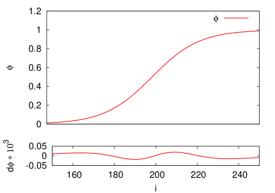
Figure 2: The bounce configuration in the one-dimensional degenerate case. The deviations from the exact analytic result are $O(10^{-4})$.

$$V(\phi)=2(\phi-1)^{2}\phi^{2}.$$ (26)

The resulting configuration and the deviation from the exact analytic result are plotted in Fig. 2.

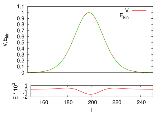
Figure 3: Potential $V$ and kinetic energy $E_{\textrm{kin}}$ of the one-dimensional configuration. The total energy $E=E_{\textrm{kin}}-V$ is conserved up to $0.1\%$.

The deviation from the exact solution is $O(10^{-4})$ and mostly due to the finite lattice spacing. Another test is provided by the kinetic energy that should vanish in the limits $\rho\to 0$ and $\rho\to T$. This was not enforced by the boundary conditions since the start and end-point of the configuration are used as boundary conditions of the discretized action, as given in Eq. (16) or Eq. (25). In addition one can analyze the conservation of energy. These tests are displayed in Fig. 3.

In the second example, a non-degenerate potential for the multi scalar case is analyzed, namely

$$V(\phi)=16(\phi_{1}-1)^{2}\phi_{1}^{2}+2\,\phi_{2}^{2}+c_{1}\,\phi_{1}+c_{2}\,\phi_{2}\phi_{1}(\phi_{1}-1).$$ (27)

The third term dissolves the degeneracy of the minima and is chosen to be rather small ($c_{1}=-0.1$). The last term gives a non-trivial dynamics in the $\phi_{2}$ direction ($c_{2}=8.0$). The numerical results are depicted in Figs. 4 and 5.

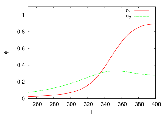
Figure 4: The bounce configuration in the two-dimensional non-degenerate case. The exponentially decreasing tail $[0,250]$ has been cut off.

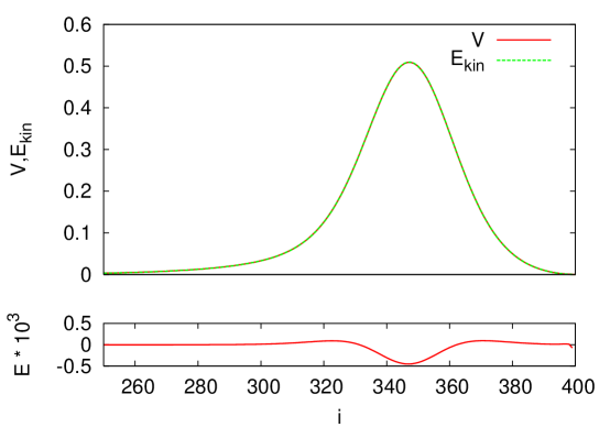
Figure 5: Potential $V$ and kinetic energy $E_{\textrm{kin}}$ of the two-dimensional configuration. The total energy $E=E_{\textrm{kin}}-V$ is conserved up to $0.1\%$. The exponentially decreasing tail $[0,250]$ has again been cut off.

The results show the expected exponential behavior close to $\phi_{-}$ and a parabolic shape near $\phi_{b}$. The energy is again conserved up to the per mille level. Especially the parabolic shape with $\partial_{\rho}\phi=0$ at the bounce point $\phi_{b}$ in Fig. 4 is a clear indication of the high precision of our numerical approach, since because of the lift of the potential in Eq. (21), the kinetic energy is there $O(\epsilon)$.

Note that the shape of the field $\phi_{2}$ is not of the usual hyperbolic tangent form, and not even monotonically increasing; hence one cannot obtain a good estimate of the bounce configuration by minimizing the action with respect to a specific ansatz, as was done in Ref. john .

V Continuation to the Damped Case

To perform the continuation from the undamped case ($\alpha=1$) to the damped case, a numerical method to solve the discretized version of Eq. (11) with the boundary conditions as given in Eqs. (3) and (4) is needed. In the present work the following discretized form of the EoM has been used:

$$\frac{\phi_{i+1}-2\phi_{i}+\phi_{i-1}}{d\rho^{2}}+\frac{\alpha-1}{(i+\Delta i)d\rho}\frac{\phi_{i+1}-\phi_{i-1}}{2\,d\rho}=\nabla V(\phi_{i}),\quad i\in[1,n-1],$$ (28)

with the boundary conditions

$$\phi_{0}=\phi_{1},\quad\phi_{n}=\phi_{-},$$ (29)

where $\phi_{i}$ constitutes the one-dimensional lattice $(i\in[0,n])$. This discretization has the virtue to be derived from the energy functional

$$H=\sum_{i}i^{2}V(\phi_{i})+\sum_{i}(i^{2}+i)\frac{(\phi_{i+1}-\phi_{i})^{2}}{2d\rho^{2}}$$ (30)

and reproduces the continuum energy with an error of $O(d\rho^{2})$.

The offset parameter $\Delta i$ has been introduced to improve the performance of the algorithm, since an initial value of $\Delta i=0$ can easily lead to a pathological behavior close to $i=0$. Finally, this parameter has to be sent to zero.

One way to obtain a solution of this system, is to use the method of squared equations of motion, as was done in Refs. seco ; john . However, since the algorithm in the last sections provides fairly good estimates $\tilde{\phi}_{i}$ of the solution, we pursue another possibility. Using the Taylor expansion of the gradient field

$$\nabla V(\phi_{i})\approx\nabla V(\tilde{\phi}_{i})+(\phi_{i}-\tilde{\phi}_{i})\cdot\nabla(\nabla V(\tilde{\phi}_{i})),$$ (31)

we can linearize the system of equations and iteratively solve the equations by inversion of the linear system. Since the matrix corresponding to this system of equations is band diagonal, its inversion is easily performed. The original system of equations in Eq. (28) is then solved iteratively by using the linearized system. Notice that the original potential is used and not the modified potential that has been utilized in the minimization of the action in the last section.

This method has been applied to the non-degenerate example of the last section and the results are briefly displayed in the following. Starting point of the continuation are the damping parameter $\alpha=1$, an offset $\Delta i=300$, a time scale $dt=0.0158$, and a lattice of size $n=400$. As initial configuration, the one generated by the improved-potential method is used, as discussed in the last section.

The parameter $\alpha$ is increased by steps of size $\delta\alpha=5\times 10^{-3}$ and the linear system in Eq. (28) is solved iteratively for each parameter set and some obtained configurations are plotted in Fig. 6. The contour of the potential and several trajectories are depicted in Fig. 7.

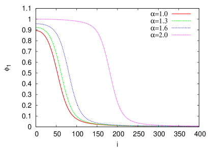
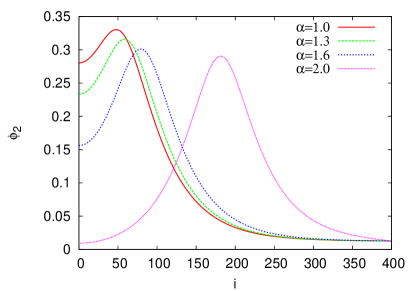
Figure 6: The fields $\phi_{1}$ and $\phi_{2}$ during the continuation for several values of $\alpha$ and $\Delta i=300$.

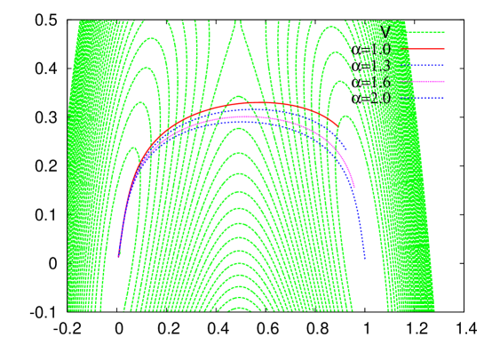
Figure 7: Contour plot of the potential and several trajectories.

As soon as the size of the bubble

$$\bar{\rho}=(\alpha-1)\,\frac{\tilde{S}_{1}}{\delta V}-\Delta i\,dt,$$ (32)

is larger than the wall thickness, an increase in $\alpha$ or a decrease in $\Delta i$ results almost only in a translation of the configuration. If this translation is anticipated, a faster continuation in the parameters $\alpha$ and $\Delta i$ becomes possible.

Since solving the linearized system of equations is not very time consuming, the accuracy of the result is in principle only limited by the finite size of the lattice and the accuracy of the numerical representation. This can be demonstrated by increasing the number of lattice sites and the results are summarized in Table 1. The relative error in the action $S_{3}$ behaves as expected as $O(\delta\rho^{2})$ and reaches approximately $7\times 10^{-6}$ for the largest lattice that was used. Errors of $O(\delta\rho^{4})$ can be obtained by extrapolation of the action to vanishing $\delta\rho$. In comparison, using the method of squared EoM or one of the algorithms of Ref. Cline:1999wi is much more time consuming and leads to inferior accuracy.

lattice sites	$S_{3}$	$\Delta S_{3}$
100	725.819
200	726.957	1.137
400	727.239	0.282
800	727.309	0.070
1600	727.326	0.017

Table 1: The action $S_{3}$ for different numbers of lattice sites. The change in the action $\Delta S_{3}$ behaves as $O(\delta\rho^{2})$. The error of the largest lattice can be estimated to be $5\times 10^{-3}$ what corresponds to a relative error of $7\times 10^{-6}$.

VI Conclusion

We presented a numerically stable and easily implemented algorithm to determine properties of phase transitions with several scalar fields. We demonstrated our approach in the simplest one-dimensional and in a non-trivial two-dimensional example. The approach we suggest converges with high precision to the bounce configuration. During the minimization neither oscillatory nor unphysical solutions have been encountered, in contrast to the approach followed in Ref. john .

Our approach was based on a procedure consisting of two steps. First, we determined the bounce solution in the undamped case, using a novel algorithm. Secondly, a smooth continuation was performed to the physical case, turning on the damping term in the EoM. Note that the sole purpose of the undamped solution is to serve as an initial configuration for the continuation. In contrast to the configuration without damping, the damped configuration usually shares more characteristics with the typical solution in the degenerate case, namely a bubble size much larger than the bubble wall thickness and an exponential behavior close to both maxima. Hence the action determined in the thin-wall regime as given in Eq. (14) is typically more accurate than using the configuration of the undamped case in the action.

The main advantage of our approach, besides the very high accuracy, is the large range of applicability. The convergence of our algorithm does not rely on a good anticipation of the bounce and is hence well suited to treat multi dimensional phase transition problems. In a forthcoming publication the method we presented will be used to analyze the electroweak phase transition in the nMSSM forthcomming .

References

- (1) J. S. Langer, “Theory of the condensation point,” Ann. Phys. 41 (1967) 108 [Ann. Phys. 281 (2000) 941].
- (2) J. S. Langer, “Statistical theory of the decay of metastable states,” Ann. Phys. 54 (1969) 258.
- (3) S. R. Coleman, “The fate of the false vacuum. 1. Semiclassical theory,” Phys. Rev. D 15 (1977) 2929 [Erratum ibid. D 16 (1977) 1248].
- (4) C. G. Callan and S. R. Coleman, “The fate of the false vacuum. 2. First quantum corrections,” Phys. Rev. D 16 (1977) 1762.
- (5) I. Affleck, “Quantum statistical metastability,” Phys. Rev. Lett. 46 (1981) 388.
- (6) A. D. Linde, “On the vacuum instability and the Higgs meson mass,” Phys. Lett. B 70 (1977) 306.
- (7) A. D. Linde, “Decay of the false vacuum at finite temperature,” Nucl. Phys. B 216 (1983) 421 [Erratum ibid. B 223 (1983) 544].
- (8) V. A. Kuzmin, V. A. Rubakov and M. E. Shaposhnikov, “On the anomalous electroweak baryon number nonconservation in the early Universe,” Phys. Lett. B 155 (1985) 36.
- (9) M. Carena, M. Quiros, M. Seco and C. E. M. Wagner, “Improved results in supersymmetric electroweak baryogenesis,” Nucl. Phys. B 650 (2003) 24 [arXiv:hep-ph/0208043].
- (10) M. Carena, J. M. Moreno, M. Quiros, M. Seco and C. E. M. Wagner, “Supersymmetric CP-violating currents and electroweak baryogenesis,” Nucl. Phys. B 599 (2001) 158 [arXiv:hep-ph/0011055].
- (11) T. Konstandin, T. Prokopec, M. G. Schmidt and M. Seco, “MSSM electroweak baryogenesis and flavour mixing in transport equations,” Nucl. Phys. B 738 (2006) 1 [arXiv:hep-ph/0505103].
- (12) A. T. Davies, C. D. Froggatt and R. G. Moorhouse, “Electroweak Baryogenesis in the Next to Minimal Supersymmetric Model,” Phys. Lett. B 372 (1996) 88 [arXiv:hep-ph/9603388].
- (13) M. Bastero-Gil, C. Hugonie, S. F. King, D. P. Roy and S. Vempati, “Does LEP prefer the NMSSM?”, Phys. Lett. B 489 (2000) 359 [arXiv:hep-ph/0006198].
- (14) A. Menon, D. E. Morrissey and C. E. M. Wagner, “Electroweak baryogenesis and dark matter in the nMSSM,” Phys. Rev. D 70 (2004) 035005 [arXiv:hep-ph/0404184].
- (15) S. J. Huber and M. G. Schmidt, “Electroweak baryogenesis: Concrete in a SUSY model with a gauge singlet,” Nucl. Phys. B 606 (2001) 183 [arXiv:hep-ph/0003122].
- (16) J. Kang, P. Langacker, T. j. Li and T. Liu, “Electroweak baryogenesis in a supersymmetric U(1)’ model,” Phys. Rev. Lett. 94 (2005) 061801 [arXiv:hep-ph/0402086].
- (17) J. M. Cline, K. Kainulainen and A. P. Vischer, “Dynamics of two Higgs doublet CP violation and baryogenesis at the electroweak phase transition,” Phys. Rev. D 54 (1996) 2451 [arXiv:hep-ph/9506284].
- (18) J. M. Cline and P. A. Lemieux, “Electroweak phase transition in two Higgs doublet models,” Phys. Rev. D 55 (1997) 3873 [arXiv:hep-ph/9609240].
- (19) A. Strumia, N. Tetradis and C. Wetterich, “The region of validity of homogeneous nucleation theory,” Phys. Lett. B 467 (1999) 279 [arXiv:hep-ph/9808263].
- (20) G. W. Anderson and L. J. Hall, “The electroweak phase transition and baryogenesis,” Phys. Rev. D 45 (1992) 2685.
- (21) M. E. Shaposhnikov, “Possible appearance of the baryon asymmetry of the Universe in an electroweak theory,” JETP Lett. 44 (1986) 465 [Pisma Zh. Eksp. Teor. Fiz. 44 (1986) 364].
- (22) M. Laine and K. Rummukainen, “A strong electroweak phase transition up to m(H) approx. 105 GeV,” Phys. Rev. Lett. 80 (1998) 5259 [arXiv:hep-ph/9804255].
- (23) M. Laine and K. Rummukainen, “The MSSM electroweak phase transition on the lattice,” Nucl. Phys. B 535 (1998) 423 [arXiv:hep-lat/9804019].
- (24) G. V. Dunne and H. Min, “Beyond the thin-wall approximation: Precise numerical computation of prefactors in false vacuum decay,” arXiv:hep-th/0511156.
- (25) J. Baacke and G. Lavrelashvili, “One-loop corrections to the metastable vacuum decay,” Phys. Rev. D 69 (2004) 025009 [arXiv:hep-th/0307202].
- (26) S. R. Coleman, “Quantum tunneling and negative eigenvalues,” Nucl. Phys. B 298 (1988) 178.
- (27) M. Claudson, L. J. Hall and I. Hinchliffe, “Low-energy supergravity: False vacua and vacuous predictions,” Nucl. Phys. B 228 (1983) 501.
- (28) A. Kusenko, “Improved action method for analyzing tunneling in quantum field theory,” Phys. Lett. B 358 (1995) 51 [arXiv:hep-ph/9504418].
- (29) J. M. Moreno, M. Quiros and M. Seco, “Bubbles in the supersymmetric standard model,” Nucl. Phys. B 526 (1998) 489 [arXiv:hep-ph/9801272].
- (30) P. John, “Bubble wall profiles with more than one scalar field: A numerical approach,” Phys. Lett. B 452 (1999) 221 [arXiv:hep-ph/9810499].
- (31) J. M. Cline, G. D. Moore and G. Servant, “Was the electroweak phase transition preceded by a color broken phase?”, Phys. Rev. D 60 (1999) 105035 [arXiv:hep-ph/9902220].
- (32) A. Kusenko, “Tunneling in quantum field theory with spontaneous symmetry breaking,” Phys. Lett. B 358 (1995) 47 [arXiv:hep-ph/9506386].
- (33) S. Huber, T. Konstandin, T. Prokopec and M. G. Schmidt, “Electroweak phase transition and baryogenesis in the nMSSM”. In preparation.