TUM-HEP-600/05

IPPP/05/74

DCPT/05/148

TTP06-06

FERMILAB-PUB-05-512-T

ZU-TH 23/05

hep-ph/0603079

Charm Quark Contribution to $K^{+}\to\pi^{+}\nu\bar{\nu}$

at Next-to-Next-to-Leading Order

Andrzej J. Buras^a, Martin Gorbahn^b,c,

Ulrich Haisch^d,e and Ulrich Nierste^c,d

Abstract

We calculate the complete next-to-next-to-leading order QCD corrections to the charm contribution of the rare decay $K^{+}\to\pi^{+}\nu\bar{\nu}$. We encounter several new features, which were absent in lower orders. We discuss them in detail and present the results for the two-loop matching conditions of the Wilson coefficients, the three-loop anomalous dimensions, and the two-loop matrix elements of the relevant operators that enter the next-to-next-to-leading order renormalization group analysis of the $Z$-penguin and the electroweak box contribution. The inclusion of the next-to-next-to-leading order QCD corrections leads to a significant reduction of the theoretical uncertainty from $\pm 9.8\%$ down to $\pm 2.4\%$ in the relevant parameter $P_{c}(X)$, implying the leftover scale uncertainties in ${\cal B}(K^{+}\to\pi^{+}\nu\bar{\nu})$ and in the determination of $|V_{td}|$, $\sin 2\beta$, and $\gamma$ from the $K\to\pi\nu\bar{\nu}$ system to be $\pm 1.3\%$, $\pm 1.0\%$, $\pm 0.006$, and $\pm 1.2^{\circ}$, respectively. For the charm quark $\overline{\rm MS}$ mass $m_{c}(m_{c})=\left(1.30\pm 0.05\right)\!\!{\rm\ GeV}$ and $|V_{us}|=0.2248$ the next-to-leading order value $P_{c}(X)=0.37\pm 0.06$ is modified to $P_{c}(X)=0.38\pm 0.04$ at the next-to-next-to-leading order level with the latter error fully dominated by the uncertainty in $m_{c}(m_{c})$. We present tables for $P_{c}(X)$ as a function of $m_{c}(m_{c})$ and $\alpha_{s}(M_{\scriptscriptstyle Z})$ and a very accurate analytic formula that summarizes these two dependences as well as the dominant theoretical uncertainties. Adding the recently calculated long-distance contributions we find ${\cal B}(K^{+}\to\pi^{+}\nu\bar{\nu})=\left(8.0\pm 1.1\right)\times 10^{-11}$ with the present uncertainties in $m_{c}(m_{c})$ and the Cabibbo-Kobayashi-Maskawa elements being the dominant individual sources in the quoted error. We also emphasize that improved calculations of the long-distance contributions to $K^{+}\to\pi^{+}\nu\bar{\nu}$ and of the isospin breaking corrections in the evaluation of the weak current matrix elements from $K^{+}\to\pi^{0}e^{+}\nu$ would be valuable in order to increase the potential of the two golden $K\to\pi\nu\bar{\nu}$ decays in the search for new physics.

1 Introduction

The rare decay $K^{+}\to\pi^{+}\nu\bar{\nu}$ plays together with $K_{L}\to\pi^{0}\nu\bar{\nu}$ an outstanding role in the field of flavor changing neutral current (FCNC) processes both in the standard model (SM) [1] and in all of its extensions [2, 3]. The main reason for this is its theoretical cleanness and its large sensitivity to short-distance QCD effects that can be systematically calculated using an effective field theory framework. The hadronic matrix element of this decay can be extracted, including isospin breaking corrections [4], from the accurately measured leading semileptonic decay $K^{+}\to\pi^{0}e^{+}\nu$, and the remaining long-distance contributions [5] turn out to be small [6], and in principle calculable by means of lattice QCD [7].

Consequently the SM decay rate of $K^{+}\to\pi^{+}\nu\bar{\nu}$ can be expressed almost entirely in terms of the Cabibbo-Kobayashi-Maskawa (CKM) [8] parameters, the top and the charm quark mass, and the strong coupling constant $\alpha_{s}(M_{\scriptscriptstyle Z})$ that enters the QCD corrections calculated within renormalization group (RG) improved perturbation theory. Beyond the SM additional parameters like new couplings and masses of new heavy particles will be present in the decay rate, but from the point of view of hadronic effects, the theoretical cleanness of the prediction will not be affected by these non-standard contributions.

In view of this, the theoretical uncertainties in the decay rate of $K^{+}\to\pi^{+}\nu\bar{\nu}$ are at leading order essentially only of perturbative origin and in order to be able to test the SM and its extensions to a high degree of precision it is important to evaluate the first non-trivial and higher order QCD corrections to this decay mode.

To be specific, the low-energy effective Hamiltonian for the $K\to\pi\nu\bar{\nu}$ system can be written in the SM as follows [9, 10]

$${\cal H}_{\rm eff}=\frac{4G_{F}}{\sqrt{2}}\frac{\alpha}{2\pi\sin^{2}\theta_{\scriptscriptstyle W}}\sum_{\ell=e,\mu,\tau}\left(\lambda_{c}X^{\ell}(x_{c})+\lambda_{t}X(x_{t})\right)(\bar{s}_{\scalebox{0.6}{$L$}}\gamma_{\mu}d_{\scalebox{0.6}{$L$}})(\bar{\nu_{\ell}}_{\scalebox{0.6}{$L$}}\gamma^{\mu}{\nu_{\ell}}_{\scalebox{0.6}{$L$}})\,.$$ (1)

Here $G_{F}$, $\alpha$, and $\sin^{2}\theta_{\scriptscriptstyle W}$ denote the Fermi constant, the electromagnetic coupling, and the weak mixing angle, respectively. The sum over $\ell$ extends over all lepton flavors, $\lambda_{i}=V_{is}^{\ast}V_{id}$ are the relevant CKM factors and $f_{\scalebox{0.6}{$L$}}$ are left-handed fermion fields. The dependence on the charged lepton mass is negligible for the top quark contribution. In the charm quark sector this is the case only for the electron and the muon but not for the tau lepton.

The function $X(x_{t})$ in Eq. (1) depends on the top quark $\overline{\rm MS}$ [11] mass through $x_{t}=m_{t}^{2}(\mu_{t})/M_{\scriptscriptstyle W}^{2}$. It originates from $Z$-penguin and electroweak box diagrams with an internal top quark. Sample diagrams are shown in Fig. 1. As the relevant operator has a vanishing anomalous dimension and the energy scales involved are of the order of the electroweak scale or higher, the function $X(x_{t})$ can be calculated within ordinary perturbation theory. It is known through next-to-leading order (NLO) [10, 12, 13]. The inclusion of these ${\cal O}(\alpha_{s})$ corrections allowed to reduce the $\pm 6\%$ uncertainty due to the top quark matching scale $\mu_{t}={\cal O}(m_{t})$ present in the leading order (LO) formula down to $\pm 1\%$. Consequently the reached theoretical accuracy on the top quark contribution to $K^{+}\to\pi^{+}\nu\bar{\nu}$ and in the amplitude of $K_{L}\to\pi^{0}\nu\bar{\nu}$, where only $X(x_{t})$ enters, is satisfactory.

The function $X^{\ell}(x_{c})$ in Eq. (1) relevant only for $K^{+}\to\pi^{+}\nu\bar{\nu}$ depends on the charm quark $\overline{\rm MS}$ mass through $x_{c}=m_{c}^{2}(\mu_{c})/M_{\scriptscriptstyle W}^{2}$. As now both high- and low-energy scales, namely $\mu_{\scriptscriptstyle W}={\cal O}(M_{\scriptscriptstyle W})$ and $\mu_{c}={\cal O}(m_{c})$ are involved, a complete RG analysis of this term is required. In this manner, large logarithms $\ln(\mu_{c}^{2}/\mu_{\scriptscriptstyle W}^{2})$ are resummed to all orders in $\alpha_{s}$. At LO such an analysis has been performed in [14]. The large scale uncertainty due to $\mu_{c}$ of $\pm 26\%$ in this result was a strong motivation for the NLO analysis of this contribution [9, 10].

$\begin{array}[]{c@{\hspace{15mm}}c}\scalebox{0.65}{ \begin{picture}(150.0,134.0)(30.0,-45.0) \put(0.0,0.0){} \put(0.0,0.0){} \put(0.0,0.0){} \put(0.0,0.0){} \put(0.0,0.0){} \put(0.0,0.0){} \put(0.0,0.0){} \put(0.0,0.0){} \put(0.0,0.0){} \raise-8.0pt\hbox to0.0pt{\kern 125.0pt\makebox(0.0,0.0)[]{\Large{{$Z$}}}\hss} \ignorespaces \raise 42.0pt\hbox to0.0pt{\kern 151.0pt\makebox(0.0,0.0)[]{\Large{{$u,c,t$}}}\hss} \ignorespaces \raise 42.0pt\hbox to0.0pt{\kern 58.0pt\makebox(0.0,0.0)[]{\Large{{$u,c,t$}}}\hss} \ignorespaces \raise 94.0pt\hbox to0.0pt{\kern 105.0pt\makebox(0.0,0.0)[]{\Large{{$W$}}}\hss} \ignorespaces \raise 96.0pt\hbox to0.0pt{\kern 157.0pt\makebox(0.0,0.0)[]{\Large{{$d$}}}\hss} \ignorespaces \raise 94.0pt\hbox to0.0pt{\kern 54.0pt\makebox(0.0,0.0)[]{\Large{{$s$}}}\hss} \ignorespaces \end{picture} }\hfil\hskip 42.67912pt&\scalebox{0.65}{ \begin{picture}(193.0,157.0)(17.0,-26.0) \put(0.0,0.0){} \put(0.0,0.0){} \put(0.0,0.0){} \put(0.0,0.0){} \put(0.0,0.0){} \put(0.0,0.0){} \raise 117.0pt\hbox to0.0pt{\kern 120.0pt\makebox(0.0,0.0)[]{\Large{{$W$}}}\hss} \ignorespaces \raise 118.0pt\hbox to0.0pt{\kern 186.0pt\makebox(0.0,0.0)[]{\Large{{$\nu$}}}\hss} \ignorespaces \raise 52.0pt\hbox to0.0pt{\kern 200.0pt\makebox(0.0,0.0)[]{\Large{{$e,\mu,\tau$}}}\hss} \ignorespaces \raise-13.0pt\hbox to0.0pt{\kern 120.0pt\makebox(0.0,0.0)[]{\Large{{$W$}}}\hss} \ignorespaces \raise-18.0pt\hbox to0.0pt{\kern 185.0pt\makebox(0.0,0.0)[b]{\Large{{$\nu$}}}\hss} \ignorespaces \put(0.0,0.0){} \put(0.0,0.0){} \put(0.0,0.0){} \put(0.0,0.0){} \raise 118.0pt\hbox to0.0pt{\kern 54.0pt\makebox(0.0,0.0)[]{\Large{{$s$}}}\hss} \ignorespaces \put(0.0,0.0){} \put(0.0,0.0){} \raise 52.0pt\hbox to0.0pt{\kern 42.0pt\makebox(0.0,0.0)[]{\Large{{$u,c,t$}}}\hss} \ignorespaces \raise-14.0pt\hbox to0.0pt{\kern 52.0pt\makebox(0.0,0.0)[]{\Large{{$d$}}}\hss} \ignorespaces \end{picture} }\end{array}$

Figure 1: Examples of $Z$-penguin and electroweak box diagrams that contribute both to $K^{+}\to\pi^{+}\nu\bar{\nu}$ and $K_{L}\to\pi^{0}\nu\bar{\nu}$. Here and in the following we do not display the neutrino line attached to the $Z$-boson.

Defining the phenomenologically useful parameter

$$P_{c}(X)=\frac{1}{\lambda^{4}}\left(\frac{2}{3}X^{e}(x_{c})+\frac{1}{3}X^{\tau}(x_{c})\right)\,,$$ (2)

with $\lambda=|V_{us}|$, one finds for $\lambda=0.2248$ at NLO [15]

$$P_{c}(X)=0.369\pm 0.036_{\rm theory}\pm 0.033_{m_{c}}\pm 0.009_{\alpha_{s}}\,,$$ (3)

where the parametric errors correspond to the ranges of the charm quark $\overline{\rm MS}$ mass $m_{c}(m_{c})$ and the strong coupling constant $\alpha_{s}(M_{\scriptscriptstyle Z})$ given in Tab. 4. The theoretical error summarizes uncertainties due to various scales and different methods of computing $\alpha_{s}(\mu_{c})$ from $\alpha_{s}(M_{\scriptscriptstyle Z})$. Details on how the quoted errors have been obtained will be given in Sec. 9.

Provided $P_{c}(X)$ is known with a sufficient precision, a measurement of $K^{+}\to\pi^{+}\nu\bar{\nu}$, either alone or together with one of $K_{L}\to\pi^{0}\nu\bar{\nu}$, allows for precise determinations of the CKM parameters [1]. The comparison of this standard unitarity triangle (UT) with the one from $B$-physics offers a stringent and unique test of the SM. In particular for the branching ratios ${\cal B}(K^{+}\to\pi^{+}\nu\bar{\nu})$ and ${\cal B}(K_{L}\to\pi^{0}\nu\bar{\nu})$ close to their SM predictions, one finds that a given uncertainty $\sigma(P_{c}(X))$ translates into [15]

$$\frac{\sigma\left(|V_{td}|\right)}{|V_{td}|} =\pm 0.41\,\frac{\sigma\left(P_{c}(X)\right)}{P_{c}(X)}\,,$$

$$\frac{\sigma\left(\sin 2\beta\right)}{\sin 2\beta} =\pm 0.34\,\frac{\sigma\left(P_{c}(X)\right)}{P_{c}(X)}\,,$$

$$\frac{\sigma\left(\gamma\right)}{\gamma} =\pm 0.83\,\frac{\sigma\left(P_{c}(X)\right)}{P_{c}(X)}\,,$$ (4)

with similar formulas given in [3]. Here $V_{td}$ is the element of the CKM matrix and $\beta$ and $\gamma$ are the angles in the standard UT. As the uncertainties in Eq. (3) coming from the charm quark mass and the CKM parameters should be decreased in the coming years it is also desirable to reduce the theoretical uncertainty in $P_{c}(X)$.

To this end, we extend here the NLO analysis of $P_{c}(X)$ presented in [9, 10] to the next-to-next-to-leading order (NNLO) [15]. We encounter several new features, which were absent in lower orders. First, closed quark loops in gluon propagators occur, resulting in a novel dependence of $P_{c}(X)$ on the top quark mass and in non-trivial matching corrections at the bottom quark threshold scale $\mu_{b}={\cal O}(m_{b})$. Second, the contributions from the vector component of the $Z$-boson coupling are non-trivial at NNLO and are only found to vanish in the sum of several contributions, which involve a flavor off-diagonal wave function renormalization. Third, the presence of anomalous triangle diagrams involving a top quark loop, two gluons, and a $Z$-boson makes it necessary to introduce a Chern-Simons operator [16, 17] in order to obtain the correct anomalous Ward identity of the axial-vector current [18]. The inclusion of such a Chern-Simons term is also required to compensate for the anomalous contributions from triangle diagrams with a bottom quark loop. Since all these effects arise first at NNLO, they are not included in the theoretical uncertainty quoted in Eq. (3), which has been estimated from the variation of scales and different methods of evaluating $\alpha_{s}(\mu_{c})$ from $\alpha_{s}(M_{\scriptscriptstyle Z})$. The only way to control their size is to compute them explicitly, which is a further strong motivation for our NNLO calculation.

Our paper is organized as follows. In Sec. 2 we give formulas for $P_{c}(X)$ and ${\cal B}(K^{+}\to\pi^{+}\nu\bar{\nu})$ at NNLO in a form suitable for phenomenological applications. In particular we present tables that show $P_{c}(X)$ for different values of $\alpha_{s}(M_{\scriptscriptstyle Z})$, $\mu_{c}$, and $m_{c}(m_{c})$ and we give a simple analytic formula for $P_{c}(X)$ that approximates the exact numerical result with high accuracy. Sec. 3 is meant to be a guide to the subsequent Secs. 4 to 7 that describe our calculation in detail. These sections are naturally rather technical and might be skipped by readers mainly interested in phenomenological applications of our result. Sec. 8 contains another accurate approximate formula for $P_{c}(X)$ that summarizes the dominant parametric and theoretical uncertainties. In Sec. 9 we present the numerical analysis of the NNLO formulas. In particular we analyze various scale uncertainties that are drastically reduced by going from NLO to NNLO. We present the result for ${\cal B}(K^{+}\to\pi^{+}\nu\bar{\nu})$ and ${\cal B}(K_{L}\to\pi^{0}\nu\bar{\nu})$ and we investigate the parametric and theoretical uncertainties in the determination of the CKM parameters with the latter being significantly reduced through our calculation. In the course of this section we also present results provided by the CKMfitter Group [19] and the UTfit Collaboration [20]. We conclude in Sec. 10. Some technical details as well as additional material has been relegated to the appendices.

2 Master Formulas at NNLO

2.1 Preliminaries

In this section we will present the formula for ${\cal B}(K^{+}\to\pi^{+}\nu\bar{\nu})$ based on the low-energy effective Hamiltonian given in Eq. (1) extended to include the recently calculated contributions of dimension-eight four fermion operators generated at the charm quark scale $\mu_{c}$, and of genuine long-distance contributions which can be described within the framework of chiral perturbation theory [6]. These contributions can be effectively included by adding

$$\delta P_{c,u}=0.04\pm 0.02\,,$$ (5)

to the relevant parameter $P_{c}(X)$. The quoted error in $\delta P_{c,u}$ can in principle be reduced by means of lattice QCD [7].

For completeness we will also recall the formula for ${\cal B}(K_{L}\to\pi^{0}\nu\bar{\nu})$ which we will use in Sec. 9 to obtain its updated SM value in view of the recently modified value of the top quark mass [21].

2.2 Branching Ratio for $K^{+}\to\pi^{+}\nu\bar{\nu}$

After summation over the three neutrino flavors the resulting branching ratio for $K^{+}\to\pi^{+}\nu\bar{\nu}$ can be written as [6, 9, 10]

$${\cal B}(K^{+}\to\pi^{+}\nu\bar{\nu})=\kappa_{+}\left[\left(\frac{{\rm Im}\lambda_{t}}{\lambda^{5}}X(x_{t})\right)^{2}+\left(\frac{{\rm Re}\lambda_{t}}{\lambda^{5}}X(x_{t})+\frac{{\rm Re}\lambda_{c}}{\lambda}\left(P_{c}(X)+\delta P_{c,u}\right)\right)^{2}\right]\,,$$ (6)

with

$$\kappa_{+}=r_{K^{+}}\frac{3\alpha^{2}\,{\cal B}(K^{+}\to\pi^{0}e^{+}\nu)}{2\pi^{2}\sin^{4}\theta_{\scriptscriptstyle W}}\lambda^{8}=\left(5.04\pm 0.17\right)\times 10^{-11}\left(\frac{\lambda}{0.2248}\right)^{8}\,.$$ (7)

Here the parameter $r_{K^{+}}=0.901\pm 0.027$ summarizes isospin breaking corrections in relating $K^{+}\to\pi^{+}\nu\bar{\nu}$ to $K^{+}\to\pi^{0}e^{+}\nu$ [4]. The apparent strong dependence of ${\cal B}(K^{+}\to\pi^{+}\nu\bar{\nu})$ on $\lambda$ is spurious as both $P_{c}(X)$ and $\delta P_{c,u}$ are proportional to $1/\lambda^{4}$. In quoting the value for $P_{c}(X)$ and ${\cal B}(K^{+}\to\pi^{+}\nu\bar{\nu})$ we will set $\lambda=0.2248$. $\alpha$ and $\sin^{2}\theta_{\scriptscriptstyle W}$ entering ${\cal B}(K^{+}\to\pi^{+}\nu\bar{\nu})$ are naturally evaluated at the electroweak scale [22]. Then the leading term in the heavy top expansion of the electroweak two-loop corrections to $X(x_{t})$ amounts to typically $-1\%$ for the $\overline{\rm MS}$ definition of $\alpha$ and $\sin^{2}\theta_{\scriptscriptstyle W}$ [23]. In obtaining the numerical value of Eq. (7) we have employed $\alpha=\alpha_{\overline{\rm MS}}(M_{\scriptscriptstyle Z})=1/127.9$, $\sin^{2}\theta_{\scriptscriptstyle W}=\sin^{2}\hat{\theta}_{\scriptscriptstyle W}=0.231$, and ${\cal B}(K^{+}\to\pi^{0}e^{+}\nu)=\left(4.93\pm 0.07\right)\times 10^{-2}$ [24]. We remark that in writing ${\cal B}(K^{+}\to\pi^{+}\nu\bar{\nu})$ in the form of Eq. (6) we have omitted a term proportional to $\left(X^{e}(x_{c})-X^{\tau}(x_{c})\right)^{2}$. Its effect on ${\cal B}(K^{+}\to\pi^{+}\nu\bar{\nu})$ is around $+0.2\%$.

The function $X(x_{t})$ entering Eqs. (1), (6) and (17) is given in NLO accuracy by

$$X(x_{t})=X_{0}(x_{t})+\frac{\alpha_{s}(\mu_{t})}{4\pi}X_{1}(x_{t})=\eta_{X}X_{0}(x_{t}(m_{t}))\,,$$ (8)

with

$$\eta_{X}=0.986\pm 0.009\,.$$ (9)

The contribution stemming from $Z$-penguin and electroweak box diagrams without QCD corrections reads [25]

$$X_{0}(x_{t})=-\frac{2x_{t}+x_{t}^{2}}{8(1-x_{t})}-\frac{6x_{t}-3x_{t}^{2}}{8(1-x_{t})^{2}}\ln x_{t}\,,$$ (10)

while the QCD corrections to it take the following form [10, 12, 13]

$$\begin{split}X_{1}(x_{t})&=-\frac{29x_{t}-x_{t}^{2}-4x_{t}^{3}}{3(1-x_{t})^{2}}-\frac{x_{t}+9x_{t}^{2}-x_{t}^{3}-x_{t}^{4}}{(1-x_{t})^{3}}\ln x_{t}\\ &+\frac{8x_{t}+4x_{t}^{2}+x_{t}^{3}-x_{t}^{4}}{2(1-x_{t})^{3}}\ln^{2}x_{t}-\frac{4x_{t}-x_{t}^{3}}{(1-x_{t})^{2}}{\rm Li}_{2}(1-x_{t})+8x_{t}\frac{\partial X_{0}(x_{t})}{\partial x_{t}}\ln\frac{\mu_{t}^{2}}{M_{\scriptscriptstyle W}^{2}}\,.\end{split}$$ (11)

Here ${\rm Li}_{2}(x)=-\int^{x}_{0}dt\,\ln(1-t)/t$. The explicit $\mu_{t}$-dependence of the last term in Eq. (11) cancels to the considered order the $\mu_{t}$-dependence of the leading term $X_{0}(x_{t}(\mu_{t}))$. The factor $\eta_{X}$ summarizes the NLO corrections. Its error has been obtained by varying $\mu_{t}$ in the range $60\!{\rm\ GeV}\leq\mu_{t}\leq 240\!{\rm\ GeV}$ on the left-hand side of Eq. (8) while keeping $\mu_{t}$ fixed at $m_{t}=m_{t}(m_{t})$ on the right-hand side of the same equation. The leftover $\mu_{t}$-dependence in $X(x_{t})$ is slightly below $\pm 1\%$.

The uncertainty in $X(x_{t})$ is then dominated by the experimental error in the mass of the top quark. Converting the top quark pole mass of $M_{t}=\left(172.7\pm 2.9\right)\!\!{\rm\ GeV}$ [21] at three loops to $m_{t}(M_{t})$ [26] and relating $m_{t}(M_{t})$ to $m_{t}(m_{t})=\left(163.0\pm 2.8\right)\!\!{\rm\ GeV}$ using one-loop accuracy, we find

$$X(x_{t})=1.464\pm 0.041\,.$$ (12)

The given uncertainty combines linearly an error of $\pm 0.028$ due to the error of $m_{t}(m_{t})$ and an error of $\pm 0.013$ obtained by varying $\mu_{t}$ in the range given above.

	$P_{c}(X)$
$\alpha_{s}(M_{\scriptscriptstyle Z})\hskip 4.2679pt\backslash\hskip 4.2679pt\mu_{c}\hskip 4.2679pt[\!\!{\rm\ GeV}]$	1.0	1.5	2.0	2.5	3.0
0.115	0.393	0.397	0.395	0.392	0.388
0.116	0.389	0.394	0.391	0.388	0.383
0.117	0.384	0.390	0.387	0.383	0.379
0.118	0.380	0.386	0.383	0.379	0.374
0.119	0.375	0.381	0.379	0.374	0.369
0.120	0.370	0.377	0.374	0.369	0.364
0.121	0.365	0.372	0.369	0.364	0.359
0.122	0.359	0.368	0.364	0.359	0.354
0.123	0.353	0.363	0.359	0.354	0.348

Table 1: The parameter $P_{c}(X)$ in NNLO approximation for various values of $\alpha_{s}(M_{\scriptscriptstyle Z})$ and $\mu_{c}$. In quoting the numerical values for $P_{c}(X)$ we have set $\lambda=0.2248$, $m_{t}(m_{t})=163.0\!{\rm\ GeV}$, $m_{c}(m_{c})=1.30\!{\rm\ GeV}$, $\mu_{\scriptscriptstyle W}=80.0\!{\rm\ GeV}$, and $\mu_{b}=5.0\!{\rm\ GeV}$.

Figure 2: The parameter $P_{c}(X)$ at NNLO as a function of $m_{c}(m_{c})$ (upper plot) and $\alpha_{s}(M_{\scriptscriptstyle Z})$ (lower plot). In obtaining the numerical values for $P_{c}(X)$ we have set $\lambda=0.2248$, $m_{t}(m_{t})=163.0\!{\rm\ GeV}$, $\mu_{\scriptscriptstyle W}=80.0\!{\rm\ GeV}$, $\mu_{b}=5.0\!{\rm\ GeV}$, $\mu_{c}=1.50\!{\rm\ GeV}$, $\alpha_{s}(M_{\scriptscriptstyle Z})=0.1187$ (upper plot), and $m_{c}(m_{c})=1.30\!{\rm\ GeV}$ (lower plot).

As opposed to $X(x_{t})$ the charm quark contribution, represented by the parameter $P_{c}(X)$ in Eq. (2), involves several different scales like $\mu_{\scriptscriptstyle W}$, $\mu_{b}$, and $\mu_{c}$. In order to control the size of the perturbative corrections to $P_{c}(X)$ the large logarithms associated with these scales have to be resummed to all orders in $\alpha_{s}$ using RG techniques. Keeping terms to first order in $\alpha_{s}$, the perturbative expansion of $P_{c}(X)$ has the following general structure

$$P_{c}(X)=\frac{4\pi}{\alpha_{s}(\mu_{c})}P_{c}^{(0)}(X)+P_{c}^{(1)}(X)+\frac{\alpha_{s}(\mu_{c})}{4\pi}P_{c}^{(2)}(X)\,,$$ (13)

where we have suppressed the dependence of the expansion coefficients $P_{c}^{(k)}(X)$ on the involved physical and unphysical mass scales for simplicity. The leading term $P_{c}^{(0)}(X)$ has been worked out in [14] while the NLO correction $P_{c}^{(1)}(X)$ has been calculated in [9, 10].

The main goal of the present paper is the calculation of the NNLO term $P_{c}^{(2)}(X)$. As indicated by the theoretical error in Eq. (3), the sum of the first two terms in Eq. (13) still exhibits sizable unphysical scale dependences, in particular the one on $\mu_{c}$. Besides, the NLO value of $P_{c}(X)$ depends in a non-negligible way on the method used to compute $\alpha_{s}(\mu_{c})$ from $\alpha_{s}(M_{\scriptscriptstyle Z})$ [15]. The observed numerical difference is due to higher order terms in $\alpha_{s}$ and has to be regarded as part of the theoretical error. This source of uncertainty has not been taken into account in previous NLO analyses of the charm quark contribution [3, 9, 10].

	$P_{c}(X)$
$\alpha_{s}(M_{\scriptscriptstyle Z})\hskip 4.2679pt\backslash\hskip 4.2679ptm_{c}(m_{c})\hskip 4.2679pt[\!\!{\rm\ GeV}]$	1.15	1.20	1.25	1.30	1.35	1.40	1.45
0.115	0.307	0.336	0.366	0.397	0.430	0.463	0.497
0.116	0.303	0.332	0.362	0.394	0.426	0.459	0.493
0.117	0.300	0.329	0.359	0.390	0.422	0.455	0.489
0.118	0.296	0.325	0.355	0.386	0.417	0.450	0.484
0.119	0.292	0.321	0.350	0.381	0.413	0.446	0.480
0.120	0.288	0.316	0.346	0.377	0.409	0.441	0.475
0.121	0.283	0.312	0.342	0.372	0.404	0.437	0.470
0.122	0.279	0.307	0.337	0.368	0.399	0.432	0.465
0.123	0.274	0.303	0.332	0.363	0.394	0.426	0.460

Table 2: The parameter $P_{c}(X)$ in NNLO approximation for various values of $\alpha_{s}(M_{\scriptscriptstyle Z})$ and $m_{c}(m_{c})$. In quoting the numerical values for $P_{c}(X)$ we have set $\lambda=0.2248$, $m_{t}(m_{t})=163.0\!{\rm\ GeV}$, $\mu_{\scriptscriptstyle W}=80.0\!{\rm\ GeV}$, $\mu_{b}=5.0\!{\rm\ GeV}$, and $\mu_{c}=1.50\!{\rm\ GeV}$.

As we will demonstrate in Sec. 9, the inclusion of $P_{c}^{(2)}(X)$ removes essentially the entire sensitivity of $P_{c}(X)$ on $\mu_{c}$ and on higher order terms in $\alpha_{s}$ that effect the evaluation of $\alpha_{s}(\mu_{c})$ from $\alpha_{s}(M_{\scriptscriptstyle Z})$. As a result, the final theoretical error in $P_{c}(X)$ is reduced from $\pm 9.8\%$ at NLO down to $\pm 2.4\%$ at NNLO. After our calculation the theoretical accuracy on the charm quark contribution to $K^{+}\to\pi^{+}\nu\bar{\nu}$ is thus also satisfactory.

The analytic formula for the sum of the first two terms in Eq. (13) can be found in [9, 10]. The formula for $P_{c}^{(2)}(X)$ is given in Secs. 6 to 8. Setting $\lambda=0.2248$, $m_{t}(m_{t})=163.0\!{\rm\ GeV}$, $\mu_{\scriptscriptstyle W}=80.0\!{\rm\ GeV}$, $\mu_{b}=5.0\!{\rm\ GeV}$, and $\mu_{c}=1.50\!{\rm\ GeV}$, we derive an approximate formula for $P_{c}(X)$ as a function of $m_{c}(m_{c})$ and $\alpha_{s}(M_{\scriptscriptstyle Z})$. It reads

$$P_{c}(X)=0.379\left(\frac{m_{c}(m_{c})}{1.30\!{\rm\ GeV}}\right)^{2.155}\left(\frac{\alpha_{s}(M_{\scriptscriptstyle Z})}{0.1187}\right)^{-1.417}\,,$$ (14)

and approximates the exact NNLO result with an accuracy of better than $\pm 1.0\%$ in the ranges $1.15\!{\rm\ GeV}\leq m_{c}(m_{c})\leq 1.45\!{\rm\ GeV}$ and $0.1150\leq\alpha_{s}(M_{\scriptscriptstyle Z})\leq 0.1230$.

The dependence of $P_{c}(X)$ on $m_{c}(m_{c})$ and $\alpha_{s}(M_{\scriptscriptstyle Z})$ can be seen in Fig. 2, while in Tabs. 1 and 2 we present the exact values for $P_{c}(X)$ for different values of $\alpha_{s}(M_{\scriptscriptstyle Z})$, $\mu_{c}$, and $m_{c}(m_{c})$. We observe that the $\mu_{c}$-dependence is almost negligible and the dependence on $\alpha_{s}(M_{\scriptscriptstyle Z})$ is small. On the other hand the dependence on $m_{c}(m_{c})$ is sizable. A reduction of the error in $m_{c}(m_{c})$, which is dominated by theoretical uncertainties, is thus an important goal in connection with $K^{+}\to\pi^{+}\nu\bar{\nu}$.

Figure 3: The branching ratio ${\cal B}(K^{+}\to\pi^{+}\nu\bar{\nu})$ at NNLO as a function of $m_{c}(m_{c})$ (upper plot) and $M_{t}$ (lower plot). In obtaining the numerical values for ${\cal B}(K^{+}\to\pi^{+}\nu\bar{\nu})$ we have used $\mu_{\scriptscriptstyle W}=80.0\!{\rm\ GeV}$, $\mu_{b}=5.0\!{\rm\ GeV}$, and $\mu_{c}=1.50\!{\rm\ GeV}$, and set all input parameters to their central values as given in Tab. 4.

Employing the central values of the input parameters summarized in Tab. 4, the dependence of ${\cal B}(K^{+}\to\pi^{+}\nu\bar{\nu})$ on $m_{c}(m_{c})$ is described by

$${\cal B}(K^{+}\to\pi^{+}\nu\bar{\nu})=8.15\left(\frac{m_{c}(m_{c})}{1.30\!{\rm\ GeV}}\right)^{1.19}\times 10^{-11}\,,$$ (15)

which approximates the exact NNLO result with an accuracy of almost $\pm 0.6\%$ in the range $1.15\!{\rm\ GeV}\leq m_{c}(m_{c})\leq 1.45\!{\rm\ GeV}$. Similarly, the dependence on $M_{t}$ is given by

$${\cal B}(K^{+}\to\pi^{+}\nu\bar{\nu})=8.11\left(\frac{M_{t}}{172.7\!{\rm\ GeV}}\right)^{1.46}\times 10^{-11}\,,$$ (16)

which approximates the exact NNLO result with an accuracy of better than $\pm 0.1\%$ in the range $165.0\!{\rm\ GeV}\leq M_{t}\leq 180.0\!{\rm\ GeV}$. The dependences in Eqs. (15) and (16) are exhibited in Fig. 3. We remark that the present analysis of the UT is practically independent of the exact value of the top quark mass. In obtaining both Eqs. (15) and (16) we have therefore set for simplicity ${\rm Im}\lambda_{t}$, ${\rm Re}\lambda_{t}$, and ${\rm Re}\lambda_{c}$ to their central values as given in Tab. 4. Furthermore we have used the numerical value of $P_{c}(X)$ evaluated at $\mu_{\scriptscriptstyle W}=80.0\!{\rm\ GeV}$, $\mu_{b}=5.0\!{\rm\ GeV}$, and $\mu_{c}=1.5\!{\rm\ GeV}$. A detailed numerical analysis of various uncertainties in ${\cal B}(K^{+}\to\pi^{+}\nu\bar{\nu})$ will be presented in Sec. 9.

2.3 Branching Ratio for $K_{L}\to\pi^{0}\nu\bar{\nu}$

In the case of $K_{L}\to\pi^{0}\nu\bar{\nu}$ the charm quark contribution and the long-distance effects are negligible so that the relevant branching ratio is given simply as follows [9, 10]

$${\cal B}(K_{L}\to\pi^{0}\nu\bar{\nu})=\kappa_{L}\left(\frac{{\rm Im}\lambda_{t}}{\lambda^{5}}X(x_{t})\right)^{2}\,,$$ (17)

where

$$\kappa_{L}=\kappa_{+}\frac{r_{K_{L}}}{r_{K^{+}}}\frac{\tau(K_{L})}{\tau(K^{+})}=(2.20\pm 0.07)\times 10^{-10}\left(\frac{\lambda}{0.2248}\right)^{8}\,.$$ (18)

Here we have summed over the three neutrino flavors and used $\tau(K_{L})/\tau(K^{+})=4.16\pm 0.04$ [24]. $r_{K_{L}}=0.944\pm 0.028$ is the isospin breaking correction from [4] with $\kappa_{+}$ given in Eq. (7). Due to the absence of $P_{c}(X)$ in Eq. (17), ${\cal B}(K_{L}\to\pi^{0}\nu\bar{\nu})$ is plagued only by small theoretical uncertainties coming from $\mu_{t}$ and $\kappa_{L}$. The total parametric uncertainty stemming from $m_{t}(m_{t})$ and ${\rm Im}\lambda_{t}$ is on the other hand sizeable. The latter errors should be decreased significantly in the coming years, so that a precise prediction for ${\cal B}(K_{L}\to\pi^{0}\nu\bar{\nu})$ should be possible in this decade.

2.4 Summary

As far as perturbative uncertainties are concerned, with the NNLO correction to the charm quark contribution to ${\cal B}(K^{+}\to\pi^{+}\nu\bar{\nu})$ at hand, $K^{+}\to\pi^{+}\nu\bar{\nu}$ has been put nearly on the same level as $K_{L}\to\pi^{0}\nu\bar{\nu}$. The leftover scale ambiguities are all small, so that the reached theoretical accuracy is now satisfactory in both decays. Similarly the errors due to uncertainties in $\alpha_{s}(M_{\scriptscriptstyle Z})$ and $m_{t}(m_{t})$ are small. The future of precise predictions for ${\cal B}(K^{+}\to\pi^{+}\nu\bar{\nu})$ will depend primarily on the reduction of the errors in $m_{c}(m_{c})$ and in the CKM parameters, whereas ${\cal B}(K_{L}\to\pi^{0}\nu\bar{\nu})$ is practically only affected by the uncertainties in the CKM elements. Non-negligible uncertainties arise in both cases also from the theoretical error of the isospin breaking corrections and in the case of ${\cal B}(K^{+}\to\pi^{+}\nu\bar{\nu})$ from the uncertainty associated with the long-distance corrections.

On the other hand the determination of the CKM parameters and of the UT from the $K\to\pi\nu\bar{\nu}$ system will depend on the progress in the determination of $m_{c}(m_{c})$ and the measurements of both branching ratios. Also a further reduction of the error in $|V_{cb}|$, $r_{K^{+}}$, $r_{K_{L}}$, and $\delta P_{c,u}$ would be very welcome in this respect.

3 Guide to the NNLO Calculation

In analogy to many other FCNC processes, perturbative QCD effects lead to a sizable modification of the purely electroweak contribution to $K^{+}\to\pi^{+}\nu\bar{\nu}$ by generating large logarithms of the form $L=\ln(\mu_{c}^{2}/\mu_{\scriptscriptstyle W}^{2})$. A suitable framework to achieve the necessary resummation of the logarithmic enhanced corrections is the construction of an effective field theory by integrating out the heavy degrees of freedom. In this context short-distance QCD corrections can be systematically calculated by solving the RG equation that governs the scale dependence of the Wilson coefficient functions of the relevant local operators built out of the light and massless SM fields.

As several new features, which were absent in LO and NLO, enter the RG analysis of $P_{c}(X)$ at NNLO, the actual calculation is rather involved and it is worthwhile to outline first its general structure. This will be done in this section, whereas the details of the computation of the different ingredients that are necessary to obtain the NNLO correction to $P_{c}(X)$ will be described in Secs. 4 to 7.

The key element of the RG analysis of the charm quark contribution to the $s\to d\nu\bar{\nu}$ transition is the mixing of the bilocal composite operators

$$Q^{P}_{\pm}=-i\int\!d^{4}x\hskip 2.84526ptT\big{(}Q^{c}_{\pm}(x)Q_{Z}(0)-Q^{u}_{\pm}(x)Q_{Z}(0)\big{)}\,,$$ (19)

and

$$Q^{B}=-i\int\!d^{4}x\hskip 2.84526ptT\big{(}Q^{c}_{3}(x)Q^{c}_{4}(0)-Q^{u}_{3}(x)Q^{u}_{4}(0)\big{)}\,,$$ (20)

where T denotes the usual time-ordering, into

$$Q_{\nu}=\frac{m_{c}^{2}}{g^{2}\mu^{2\epsilon}}\sum_{\ell=e,\mu,\tau}\left(\bar{s}_{\scalebox{0.6}{$L$}}\gamma_{\mu}d_{\scalebox{0.6}{$L$}}\right)\left(\bar{\nu_{\ell}}_{\scalebox{0.6}{$L$}}\gamma^{\mu}{\nu_{\ell}}_{\scalebox{0.6}{$L$}}\right)\,.$$ (21)

Here $m_{c}$ is the charm quark $\overline{\rm MS}$ mass $m_{c}(\mu)$, and the inverse powers of $g$ have been introduced for later convenience, following [9]. One may arbitrarily shift such factors from the Wilson coefficient into the definition of the operator. The factor $\mu^{-2\epsilon}$ stems from the relation ${g}_{0}=Z_{g}g\mu^{\epsilon}$, where $Z_{g}$ denotes the renormalization constant of $g$, and the fact that $Q_{\nu}$ written in terms of bare fields and parameters must be $\mu$-independent. All bare quantities will carry the subscript ${0}$ hereafter. The operators $Q_{\pm}^{q}$, $Q_{3}^{q}$, and $Q_{4}^{q}$ entering Eqs. (19) and (20) will be defined as we proceed.

Interestingly the charm quark contribution to the $s\to d\nu\bar{\nu}$ amplitude involves large logarithms even in the absence of QCD interactions, because $Q^{P}_{\pm}$ and $Q^{B}$ mix into $Q_{\nu}$ through one-loop diagrams containing no gluon. The relevant Feynman graphs can be seen in Fig. 4. Factoring out $G_{F}$ and $\alpha$ the charm quark contribution to the $s\to d\nu\bar{\nu}$ amplitude thus receives corrections of ${\cal O}(\alpha_{s}^{n}L^{n+1})$ at LO, of ${\cal O}(\alpha_{s}^{n}L^{n})$ at NLO, and of ${\cal O}(\alpha_{s}^{n}L^{n-1})$ at NNLO. This structure of large logarithms explains the peculiar expansion of $P_{c}(X)$ in Eq. (13) with the leading term being of ${\cal O}(1/\alpha_{s})$ rather than ${\cal O}(1)$.

$\begin{array}[]{c@{\hspace{15mm}}c}\scalebox{0.65}{ \begin{picture}(120.0,137.0)(45.0,-30.0) \put(0.0,0.0){} \put(0.0,0.0){} \put(0.0,0.0){} \put(0.0,0.0){} \raise 99.0pt\hbox to0.0pt{\kern 75.0pt\makebox(0.0,0.0)[]{\Large{{$\nu$}}}\hss} \ignorespaces \raise 99.0pt\hbox to0.0pt{\kern 135.0pt\makebox(0.0,0.0)[]{\Large{{$\nu$}}}\hss} \ignorespaces \raise 38.0pt\hbox to0.0pt{\kern 160.0pt\makebox(0.0,0.0)[]{\Large{{$u,c$}}}\hss} \ignorespaces \raise-22.0pt\hbox to0.0pt{\kern 75.0pt\makebox(0.0,0.0)[]{\Large{{$s$}}}\hss} \ignorespaces \raise-20.0pt\hbox to0.0pt{\kern 135.0pt\makebox(0.0,0.0)[]{\Large{{$d$}}}\hss} \ignorespaces \put(0.0,0.0){} \put(0.0,0.0){} \put(0.0,0.0){} \put(0.0,0.0){} \raise 38.0pt\hbox to0.0pt{\kern 50.0pt\makebox(0.0,0.0)[]{\Large{{$u,c$}}}\hss} \ignorespaces \end{picture} }\hfil\hskip 42.67912pt&\scalebox{0.65}{ \begin{picture}(120.0,138.0)(45.0,-30.0) \put(0.0,0.0){} \put(0.0,0.0){} \put(0.0,0.0){} \put(0.0,0.0){} \put(0.0,0.0){} \raise 100.0pt\hbox to0.0pt{\kern 75.0pt\makebox(0.0,0.0)[]{\Large{{$s$}}}\hss} \ignorespaces \raise 99.0pt\hbox to0.0pt{\kern 135.0pt\makebox(0.0,0.0)[]{\Large{{$\nu$}}}\hss} \ignorespaces \raise 39.0pt\hbox to0.0pt{\kern 170.0pt\makebox(0.0,0.0)[]{\Large{{$e,\mu,\tau$}}}\hss} \ignorespaces \raise-21.0pt\hbox to0.0pt{\kern 75.0pt\makebox(0.0,0.0)[]{\Large{{$d$}}}\hss} \ignorespaces \raise-22.0pt\hbox to0.0pt{\kern 135.0pt\makebox(0.0,0.0)[]{\Large{{$\nu$}}}\hss} \ignorespaces \put(0.0,0.0){} \put(0.0,0.0){} \put(0.0,0.0){} \raise 39.0pt\hbox to0.0pt{\kern 50.0pt\makebox(0.0,0.0)[]{\Large{{$u,c$}}}\hss} \ignorespaces \end{picture} }\end{array}$

Figure 4: One-loop diagrams in the low-energy effective theory that involve a large leading logarithms. The black squares represent the insertion of the bilocal composite operators $Q^{P}_{\pm}$ (left) and $Q^{B}$ (right). The charm quark line is open in the left diagram and in all subsequent diagrams in which the charm quark couples to $Q_{\pm}^{c}$.

Since there is no mixing between the bilocal composite operators $Q_{\pm}^{P}$ and $Q^{B}$, the RG analysis of $P_{c}(X)$ naturally splits into two parts: one for the $Z$-penguin contribution which involves $Q_{\pm}^{P}$ and one for the electroweak box contribution that brings $Q^{B}$ into play. As the structure of the $Z$-penguin is more complicated than the one of the electroweak boxes it is useful to discuss the former type of contributions first. This will be done in Sec. 6. After the detailed exposition of the $Z$-penguin contribution it is straightforward to repeat the analysis in the analogous, but somewhat simpler case of the electroweak boxes. The essential steps of this calculation will be discussed in Sec. 7.

The main components of the calculations of Secs. 6 and 7 performed here at the NNLO level are: $i)$ the two-loop ${\cal O}(\alpha_{s}^{2})$ corrections to the initial conditions of the relevant Wilson coefficients at $\mu_{\scriptscriptstyle W}$, $ii)$ the three-loop ${\cal O}(\alpha_{s}^{3})$ ADM describing the mixing of the associated physical operators, $iii)$ the two-loop ${\cal O}(\alpha_{s}^{2})$ threshold corrections to the Wilson coefficients at $\mu_{b}$, and $iv)$ the two-loop matrix elements ${\cal O}(\alpha_{s}^{2})$ of the relevant operators at $\mu_{c}$.

The current-current operators $Q_{\pm}^{q}$ which enters the bilocal composite operator $Q^{P}_{\pm}$ are familiar from the non-leptonic $|\Delta S|=1$ transitions. As their mixing under renormalization is not affected by the presence of the other operators, it is convenient to perform their RG analysis before discussing the $Z$-penguin contribution itself. This calculation involves the first three aforementioned steps as we will explain in Sec. 4.

The second ingredient of the bilocal composite operator $Q^{P}_{\pm}$ is the neutral-current operator $Q_{Z}$, which describes the interactions of neutrinos and quarks mediated by $Z$-boson exchange. It is a linear combination of the usual vector and axial-vector couplings of the left-handed neutrino current to quarks, and a Chern-Simons operator that describes the coupling of neutrinos to two and three gluons. The inclusion of the Chern-Simons operator is essential to guarantee the non-renormalization of $Q_{Z}$ to all orders in $\alpha_{s}$, which plays an important role in the RG analysis of the $Z$-penguin sector. The subleties arising in connection with $Q_{Z}$ will be reviewed in Sec. 5.1 before analyzing the $Z$-penguin contribution itself.

Finally, we will discuss the operators $Q_{3}^{q}$ and $Q_{4}^{q}$. These operators are the building blocks of the bilocal composite operator $Q^{B}$ and describe the interactions between leptons and quarks mediated by $W$-exchange. They will be briefly discussed in Sec. 5.2.

In summary, after the three preparatory sections, namely Secs. 4, 5.1, and 5.2, that discuss the dimension-six operators $Q_{\pm}^{q}$, $Q_{Z}$, $Q_{3}^{q}$, and $Q_{4}^{q}$, the actual NNLO calculation relevant for the charm quark contribution to $K^{+}\to\pi^{+}\nu\bar{\nu}$ is presented in Secs. 6 and 7 for the $Z$-penguin and the electroweak box contributions, respectively. The result of these efforts will be summarized in Sec. 8.

4 Current-Current Interactions

4.1 Effective Hamiltonian

As we are only interested in the charm quark contribution to the $s\to d\nu\bar{\nu}$ transition, we can drop the parts of the low-energy effective Hamiltonian that are proportional to the CKM factor $\lambda_{t}$. The unitarity of the CKM matrix then allows one to express all the relevant contributions in terms of one independent CKM factor, namely $\lambda_{c}$. $P_{c}(X)$ receives contributions from $Z$-penguin and electroweak box diagrams with internal charm and up quarks. Examples are depicted in Fig. 1. For scales $\mu$ in the range $\mu_{c}\leq\mu\leq\mu_{\scriptscriptstyle W}$ the four-quark interaction mediated by $W$-boson exchange is described by the effective current-current Hamiltonian

$${\cal H}_{\rm eff}^{CC}=\frac{4G_{F}}{\sqrt{2}}\lambda_{c}\sum_{i=\pm}C_{i}(\mu)\left(Q_{i}^{c}-Q_{i}^{u}\right)\,,$$ (22)

where

$$Q_{\pm}^{q}=\frac{1}{2}\left((\bar{s}_{\scalebox{0.6}{$L$}}^{\alpha}\gamma_{\mu}q_{\scalebox{0.6}{$L$}}^{\alpha})(\bar{q}_{\scalebox{0.6}{$L$}}^{\beta}\gamma^{\mu}d_{\scalebox{0.6}{$L$}}^{\beta})\pm(\bar{s}_{\scalebox{0.6}{$L$}}^{\alpha}\gamma_{\mu}q_{\scalebox{0.6}{$L$}}^{\beta})(\bar{q}_{\scalebox{0.6}{$L$}}^{\beta}\gamma^{\mu}d_{\scalebox{0.6}{$L$}}^{\alpha})\right)\,.$$ (23)

Here $\alpha$ and $\beta$ are color indices. At LO the operators in Eq. (23) renormalize multiplicatively. Beyond LO they mix into so-called evanescent operators, which vanish algebraically in $n=4$ dimensions [27, 28, 29, 30], but affect the values of the Wilson coefficients $C_{\pm}(\mu)$. These operators can be chosen in such a way that the renormalized matrix elements of $Q_{\pm}^{q}$ and its Fierz transform are the same. For this choice $Q_{\pm}^{q}$ have well-defined and distinct isospin quantum numbers and do not mix with each other at NLO and beyond. The definitions of the evanescent operators required to preserve the diagonal form of the NNLO anomalous dimension matrix (ADM) in the $Q_{\pm}^{q}$ basis can be found in App. A.1.

4.2 Initial Conditions

We now turn our attention to the calculation of the initial conditions of $Q_{\pm}^{q}$. Dropping the unnecessary flavor index $q$ we write for $i=\pm$

$$C_{i}(\mu_{\scriptscriptstyle W})=C_{i}^{(0)}(\mu_{\scriptscriptstyle W})+\frac{\alpha_{s}(\mu_{\scriptscriptstyle W})}{4\pi}C_{i}^{(1)}(\mu_{\scriptscriptstyle W})+\left(\frac{\alpha_{s}(\mu_{\scriptscriptstyle W})}{4\pi}\right)^{2}C_{i}^{(2)}(\mu_{\scriptscriptstyle W})\,,$$ (24)

where $\alpha_{s}(\mu_{\scriptscriptstyle W})$ denotes the strong coupling constant in the $\overline{\rm MS}$ scheme for five active quark flavors. The values of the coefficients $C_{\pm}^{(k)}(\mu_{\scriptscriptstyle W})$ are determined by matching Green’s functions in the full and the effective theory at $\mu_{\scriptscriptstyle W}$. In the NNLO approximation this requires the calculation of one-particle-irreducible two-loop diagrams. Sample SM graphs are displayed in Fig. 5. For what concerns the regularization of infrared (IR) divergences we follow the procedure outlined for example in [31, 32], which consists in using dimensional regularization for both IR and ultraviolet (UV) divergences. While the former singularities are removed by renormalization, the latter poles cancel out in the difference between the full and the effective theory amplitudes. For detailed descriptions of higher-order matching calculations of strong and electroweak corrections applying the latter method we refer the interested reader to [32, 33, 34].

$\begin{array}[]{c@{\hspace{10mm}}c}\scalebox{0.65}{ \begin{picture}(180.0,144.0)(30.0,-31.0) \put(0.0,0.0){} \put(0.0,0.0){} \put(0.0,0.0){} \put(0.0,0.0){} \put(0.0,0.0){} \put(0.0,0.0){} \put(0.0,0.0){} \put(0.0,0.0){} \put(0.0,0.0){} \put(0.0,0.0){} \put(0.0,0.0){} \put(0.0,0.0){} \put(0.0,0.0){} \put(0.0,0.0){} \put(0.0,0.0){} \put(0.0,0.0){} \put(0.0,0.0){} \raise 105.0pt\hbox to0.0pt{\kern 55.0pt\makebox(0.0,0.0)[]{\Large{{$s$}}}\hss} \ignorespaces \raise 99.0pt\hbox to0.0pt{\kern 120.0pt\makebox(0.0,0.0)[]{\Large{{$s$}}}\hss} \ignorespaces \raise 105.0pt\hbox to0.0pt{\kern 186.0pt\makebox(0.0,0.0)[]{\Large{{$q$}}}\hss} \ignorespaces \raise 39.0pt\hbox to0.0pt{\kern 190.0pt\makebox(0.0,0.0)[]{\Large{{$W$}}}\hss} \ignorespaces \raise 39.0pt\hbox to0.0pt{\kern 48.0pt\makebox(0.0,0.0)[]{\Large{{$t$}}}\hss} \ignorespaces \raise 39.0pt\hbox to0.0pt{\kern 102.0pt\makebox(0.0,0.0)[]{\Large{{$t$}}}\hss} \ignorespaces \raise 69.0pt\hbox to0.0pt{\kern 57.0pt\makebox(0.0,0.0)[]{\Large{{$g$}}}\hss} \ignorespaces \raise-21.0pt\hbox to0.0pt{\kern 120.0pt\makebox(0.0,0.0)[]{\Large{{$q$}}}\hss} \ignorespaces \raise 9.0pt\hbox to0.0pt{\kern 57.0pt\makebox(0.0,0.0)[]{\Large{{$g$}}}\hss} \ignorespaces \raise-31.0pt\hbox to0.0pt{\kern 55.0pt\makebox(0.0,0.0)[b]{\Large{{$q$}}}\hss} \ignorespaces \raise-31.0pt\hbox to0.0pt{\kern 185.0pt\makebox(0.0,0.0)[b]{\Large{{$d$}}}\hss} \ignorespaces \end{picture} }\hfil\hskip 28.45274pt&\scalebox{0.65}{ \begin{picture}(180.0,144.0)(30.0,-31.0) \put(0.0,0.0){} \put(0.0,0.0){} \put(0.0,0.0){} \put(0.0,0.0){} \put(0.0,0.0){} \put(0.0,0.0){} \put(0.0,0.0){} \put(0.0,0.0){} \put(0.0,0.0){} \put(0.0,0.0){} \raise 105.0pt\hbox to0.0pt{\kern 55.0pt\makebox(0.0,0.0)[]{\Large{{$s$}}}\hss} \ignorespaces \raise 99.0pt\hbox to0.0pt{\kern 98.0pt\makebox(0.0,0.0)[]{\Large{{$s$}}}\hss} \ignorespaces \raise 105.0pt\hbox to0.0pt{\kern 186.0pt\makebox(0.0,0.0)[]{\Large{{$q$}}}\hss} \ignorespaces \raise 39.0pt\hbox to0.0pt{\kern 190.0pt\makebox(0.0,0.0)[]{\Large{{$W$}}}\hss} \ignorespaces \raise-21.0pt\hbox to0.0pt{\kern 120.0pt\makebox(0.0,0.0)[]{\Large{{$q$}}}\hss} \ignorespaces \raise-31.0pt\hbox to0.0pt{\kern 55.0pt\makebox(0.0,0.0)[b]{\Large{{$q$}}}\hss} \ignorespaces \raise-31.0pt\hbox to0.0pt{\kern 185.0pt\makebox(0.0,0.0)[b]{\Large{{$d$}}}\hss} \ignorespaces \put(0.0,0.0){} \put(0.0,0.0){} \put(0.0,0.0){} \put(0.0,0.0){} \put(0.0,0.0){} \put(0.0,0.0){} \put(0.0,0.0){} \raise 99.0pt\hbox to0.0pt{\kern 143.0pt\makebox(0.0,0.0)[]{\Large{{$s$}}}\hss} \ignorespaces \raise 54.0pt\hbox to0.0pt{\kern 115.0pt\makebox(0.0,0.0)[]{\Large{{$g$}}}\hss} \ignorespaces \raise 16.0pt\hbox to0.0pt{\kern 57.0pt\makebox(0.0,0.0)[]{\Large{{$g$}}}\hss} \ignorespaces \raise 62.0pt\hbox to0.0pt{\kern 57.0pt\makebox(0.0,0.0)[]{\Large{{$g$}}}\hss} \ignorespaces \end{picture} }\end{array}$

Figure 5: Sample diagrams for the ${\cal O}(\alpha_{s}^{2})$ corrections to the initial values of the Wilson coefficients of the current-current operators.

Using naive dimensional regularization (NDR) [35] with a fully anticommuting $\gamma_{5}$, we obtain for the standard choices of the Casimir invariants $C_{\scriptstyle A}=3$, $C_{\scriptstyle F}=4/3$, and five active quark flavors

$$\begin{split}C_{\pm}^{(0)}(\mu_{\scriptscriptstyle W})&=1\,,\\[11.38109pt] C_{\pm}^{(1)}(\mu_{\scriptscriptstyle W})&=\pm\frac{1}{2}\left(1\mp\frac{1}{3}\right)\left(11+6\ln\frac{\mu_{\scriptscriptstyle W}^{2}}{M_{\scriptscriptstyle W}^{2}}\right)\,,\\[2.84526pt] C_{\pm}^{(2)}(\mu_{\scriptscriptstyle W})&=-\frac{1}{3600}\left(135677\mp 124095\right)+\frac{1}{18}\left(7\pm 51\right)\pi^{2}\mp\frac{1}{2}\left(1\mp\frac{1}{3}\right)T(x_{t})\\ &-\frac{5}{36}\left(11\mp 249\right)\ln\frac{\mu_{\scriptscriptstyle W}^{2}}{M_{\scriptscriptstyle W}^{2}}+\frac{1}{6}\left(7\pm 51\right)\ln^{2}\frac{\mu_{\scriptscriptstyle W}^{2}}{M_{\scriptscriptstyle W}^{2}}\,.\end{split}$$ (25)

The function $T(x_{t})$ depends on the top quark $\overline{\rm MS}$ mass via $x_{t}=m_{t}^{2}(\mu_{\scriptscriptstyle W})/M_{\scriptscriptstyle W}^{2}$. It originates from SM diagrams like the one shown on the left of Fig. 5. Subtracting the corresponding terms in the gluon propagator in the momentum-space subtraction scheme at $q^{2}=0$, which ensures that $\alpha_{s}(\mu_{\scriptscriptstyle W})$ is continuous at the top quark threshold $\mu_{\scriptscriptstyle W}$, we find

$$\begin{split}T(x_{t})&=\frac{112}{9}+32x_{t}+\left(\frac{20}{3}+16x_{t}\right)\ln x_{t}\\ &-\left(8+16x_{t}\right)\sqrt{4x_{t}-1}\,{\rm Cl}_{2}\left(2\arcsin\left(\frac{1}{2\sqrt{x_{t}}}\right)\right)\,,\end{split}$$ (26)

where ${\rm Cl}_{2}(x)={\rm Im}({\rm Li}_{2}(e^{ix}))$. As far as the one-loop initial conditions, namely $C_{\pm}^{(1)}(\mu_{\scriptscriptstyle W})$ are concerned, our results agree with those of [27, 36]. They also agree with the results obtained in [37, 38] after a transformation to our renormalization scheme specified by Eqs. (A.2). The general formalism of a change of renormalization scheme discussed in detail in [39] can also be used to verify that our result for the two-loop initial conditions $C_{\pm}^{(2)}(\mu_{\scriptscriptstyle W})$ coincides with the findings of [32]. This is shown in App. A.2.

4.3 Anomalous Dimensions

The Wilson coefficients are evolved from $\mu_{\scriptscriptstyle W}$ down to the relevant low-energy scale $\mu$ with the help of the RG equation. In this way, large logarithms of the form $\ln(\mu^{2}/\mu_{\scriptscriptstyle W}^{2})$ are resummed to all orders in $\alpha_{s}$. In mass-independent renormalization schemes like $\overline{\rm MS}$ the RG equation is given by

$$\mu\frac{d}{d\mu}C_{i}(\mu)=\gamma_{ji}(\mu)C_{j}(\mu)\,,$$ (27)

where $\gamma_{ji}(\mu)$ is the entry of the ADM describing the mixing of $Q_{j}$ into $Q_{i}$. In the case of $Q^{q}_{\pm}$ we will denote the diagonal entries of $\hat{\gamma}(\mu)$ by $\gamma_{\pm}(\mu)$.

$\begin{array}[]{c@{\hspace{15mm}}c}\scalebox{0.65}{ \begin{picture}(160.0,141.0)(25.0,-52.0) \put(0.0,0.0){} \put(0.0,0.0){} \put(0.0,0.0){} \put(0.0,0.0){} \raise-4.0pt\hbox to0.0pt{\kern 105.0pt\makebox(0.0,0.0)[]{\Large{{$Q^{q}_{\pm}$}}}\hss} \ignorespaces \put(0.0,0.0){} \put(0.0,0.0){} \put(0.0,0.0){} \raise 21.0pt\hbox to0.0pt{\kern 40.0pt\makebox(0.0,0.0)[]{\Large{{$g$}}}\hss} \ignorespaces \put(0.0,0.0){} \raise 65.0pt\hbox to0.0pt{\kern 105.0pt\makebox(0.0,0.0)[]{\Large{{$g$}}}\hss} \ignorespaces \put(0.0,0.0){} \put(0.0,0.0){} \put(0.0,0.0){} \put(0.0,0.0){} \put(0.0,0.0){} \put(0.0,0.0){} \put(0.0,0.0){} \put(0.0,0.0){} \put(0.0,0.0){} \put(0.0,0.0){} \put(0.0,0.0){} \put(0.0,0.0){} \put(0.0,0.0){} \raise 21.0pt\hbox to0.0pt{\kern 170.0pt\makebox(0.0,0.0)[]{\Large{{$g$}}}\hss} \ignorespaces \raise 81.0pt\hbox to0.0pt{\kern 60.0pt\makebox(0.0,0.0)[]{\Large{{$s$}}}\hss} \ignorespaces \raise 81.0pt\hbox to0.0pt{\kern 150.0pt\makebox(0.0,0.0)[]{\Large{{$q$}}}\hss} \ignorespaces \raise-44.0pt\hbox to0.0pt{\kern 58.0pt\makebox(0.0,0.0)[]{\Large{{$q$}}}\hss} \ignorespaces \raise-42.0pt\hbox to0.0pt{\kern 150.0pt\makebox(0.0,0.0)[]{\Large{{$d$}}}\hss} \ignorespaces \end{picture} }\hfil\hskip 42.67912pt&\scalebox{0.65}{ \begin{picture}(165.0,141.0)(20.0,-52.0) \put(0.0,0.0){} \put(0.0,0.0){} \put(0.0,0.0){} \put(0.0,0.0){} \put(0.0,0.0){} \raise-4.0pt\hbox to0.0pt{\kern 105.0pt\makebox(0.0,0.0)[]{\Large{{$Q^{q}_{\pm}$}}}\hss} \ignorespaces \put(0.0,0.0){} \put(0.0,0.0){} \put(0.0,0.0){} \put(0.0,0.0){} \put(0.0,0.0){} \put(0.0,0.0){} \put(0.0,0.0){} \put(0.0,0.0){} \raise 21.0pt\hbox to0.0pt{\kern 85.0pt\makebox(0.0,0.0)[]{\Large{{$f$}}}\hss} \ignorespaces \raise 21.0pt\hbox to0.0pt{\kern 35.0pt\makebox(0.0,0.0)[]{\Large{{$f$}}}\hss} \ignorespaces \raise-9.0pt\hbox to0.0pt{\kern 43.0pt\makebox(0.0,0.0)[]{\Large{{$g$}}}\hss} \ignorespaces \raise 51.0pt\hbox to0.0pt{\kern 43.0pt\makebox(0.0,0.0)[]{\Large{{$g$}}}\hss} \ignorespaces \put(0.0,0.0){} \put(0.0,0.0){} \put(0.0,0.0){} \put(0.0,0.0){} \put(0.0,0.0){} \put(0.0,0.0){} \put(0.0,0.0){} \put(0.0,0.0){} \raise 21.0pt\hbox to0.0pt{\kern 170.0pt\makebox(0.0,0.0)[]{\Large{{$g$}}}\hss} \ignorespaces \raise-44.0pt\hbox to0.0pt{\kern 58.0pt\makebox(0.0,0.0)[]{\Large{{$q$}}}\hss} \ignorespaces \raise-42.0pt\hbox to0.0pt{\kern 150.0pt\makebox(0.0,0.0)[]{\Large{{$d$}}}\hss} \ignorespaces \raise 81.0pt\hbox to0.0pt{\kern 60.0pt\makebox(0.0,0.0)[]{\Large{{$s$}}}\hss} \ignorespaces \raise 81.0pt\hbox to0.0pt{\kern 150.0pt\makebox(0.0,0.0)[]{\Large{{$q$}}}\hss} \ignorespaces \end{picture} }\end{array}$

Figure 6: Sample diagrams for the ${\cal O}(\alpha_{s}^{3})$ mixing among the current-current operators. The fermion loop in the right Feynman graph contains $f$ active quark flavors.

In the NNLO approximation the ADM has the following perturbative expansion

$$\hat{\gamma}(\mu)=\frac{\alpha_{s}(\mu)}{4\pi}\hat{\gamma}^{(0)}+\left(\frac{\alpha_{s}(\mu)}{4\pi}\right)^{2}\hat{\gamma}^{(1)}+\left(\frac{\alpha_{s}(\mu)}{4\pi}\right)^{3}\hat{\gamma}^{(2)}\,,$$ (28)

where the coefficients $\hat{\gamma}^{(k)}$ can be extracted from the one-, two-, and three-loop QCD renormalization constants in the effective theory. The renormalization matrices are found by calculating amputated Green’s functions with single insertions of $Q^{q}_{\pm}$ up to three loops. Sample diagrams are shown in Fig. 6. The corresponding amplitudes are evaluated using the method that has been described in [40, 41, 42]. We keep the gauge parameter arbitrary and find it to cancel from $\hat{\gamma}^{(k)}$, which provides a powerful check of our calculation. To distinguish between IR and UV divergences, we introduce a common mass $M$ for all fields and expand all loop integrals in inverse powers of $M$. This makes the calculation of the UV divergences possible at three loops, as $M$ becomes the only relevant internal scale, and three-loop tadpole integrals with a single non-zero mass are known [41, 43]. Comprehensive discussions of the technical details of the renormalization of the effective theory and the actual calculation of the operator mixing are given in [40, 42].

While $\gamma^{(0)}_{\pm}$ is renormalization-scheme independent, $\gamma^{(1)}_{\pm}$ and $\gamma^{(2)}_{\pm}$ are not. In the NDR scheme supplemented by the definition of evanescent operators given in Eqs. (A.2), we obtain for $C_{\scriptstyle A}=3$, $C_{\scriptstyle F}=4/3$, and an arbitrary number of active quark flavors $f$

$$\begin{split}\gamma_{\pm}^{(0)}&=\pm 6\left(1\mp\frac{1}{3}\right)\,,\\[2.84526pt] \gamma_{\pm}^{(1)}&=\left(-\frac{21}{2}\pm\frac{2}{3}f\right)\left(1\mp\frac{1}{3}\right)\,,\\[2.84526pt] \gamma_{\pm}^{(2)}&=\frac{1}{300}\left(349049\pm 201485\right)-\frac{1}{1350}\left(115577\mp 9795\right)f\\[2.84526pt] &\mp\frac{130}{27}\left(1\mp\frac{1}{3}\right)f^{2}\mp\left(672+80\left(1\mp\frac{1}{3}\right)f\right)\zeta(3)\,.\end{split}$$ (29)

Here $\zeta(x)$ is the Riemann zeta function with the value $\zeta(3)\approx 1.20206$. Again, we find agreement with the one- and two-loop results of [27, 36], and therefore also with the findings of [37, 38, 42] that were obtained in different renormalization schemes. We also confirm the three-loop results presented recently [39]. The explicit formulas that allow the conversion of the latter anomalous dimensions to our scheme can be found in App. A.2.

4.4 Threshold Corrections

In order to compute the Wilson coefficients for scales $\mu$ much lower than $\mu_{\scriptscriptstyle W}$ a proper matching between effective theories containing $f$ and $f-1$ active quark flavors has to be performed each time one passes through a flavor threshold. It is achieved by requiring that the Green’s functions in both effective theories are the same at the point $\mu_{f}={\cal O}(m_{f})$ where the quark with mass $m_{f}$ is integrated out. This equality translates into

$$\big{\langle}\vec{Q}^{f-1}(\mu_{f})\big{\rangle}^{T}\vec{C}^{f-1}(\mu_{f})=\big{\langle}\vec{Q}^{f}(\mu_{f})\big{\rangle}^{T}\vec{C}^{f}(\mu_{f})\,,$$ (30)

where the labels $f$ and $f-1$ indicate to which effective theory the variable belongs. Including corrections up to NNLO we write

$$\big{\langle}\vec{Q}^{f}(\mu_{f})\big{\rangle}^{T}=\big{\langle}\vec{Q}^{f}\big{\rangle}^{(0)T}\left(\hat{1}+\frac{\alpha_{s}^{f}(\mu_{f})}{4\pi}\hat{r}^{f(1)\,T}(\mu_{f})+\left(\frac{\alpha_{s}^{f}(\mu_{f})}{4\pi}\right)^{2}\hat{r}^{f(2)\,T}(\mu_{f})\right)\,,$$ (31)

where $\langle\vec{Q}^{f}\big{\rangle}^{(0)}$, $\hat{r}^{f(1)}(\mu_{f})$, and $\hat{r}^{f(2)}(\mu_{f})$ codify the tree-level, one-, and two-loop matrix element of the column vector $\vec{Q}^{f}$ containing the relevant physical operators. The other quantities entering Eq. (30) can be expanded in a similar fashion.

Another subtlety arises when working in mass-independent renormalization schemes, because the matching conditions connecting the strong coupling constants of the effective theories with $f$ and $f-1$ active quark flavors are non-trivial in such schemes. In particular, in the $\overline{\rm MS}$ scheme one has in the NNLO approximation [44, 45]

$$\begin{split}\alpha_{s}^{f-1}(\mu_{f})&=\alpha_{s}^{f}(\mu_{f})\left(1-\frac{\alpha_{s}^{f}(\mu_{f})}{4\pi}\frac{2}{3}\ln\frac{\mu_{f}^{2}}{m_{f}^{2}}\right.\\ &\left.+\left(\frac{\alpha_{s}^{f}(\mu_{f})}{4\pi}\right)^{2}\left(\frac{22}{9}-\frac{38}{3}\ln\frac{\mu_{f}^{2}}{m_{f}^{2}}+\frac{4}{9}\ln^{2}\frac{\mu_{f}^{2}}{m_{f}^{2}}\right)\right)\,,\end{split}$$ (32)

where $m_{f}=m_{f}(m_{f})$ denotes the quark $\overline{\rm MS}$ mass. Of course, the appearance of both logarithmic and finite corrections can be avoided by adjusting the renormalization scheme so that $\alpha_{s}^{f-1}(\mu_{f})=\alpha_{s}^{f}(\mu_{f})$. While this does not affect the physical amplitudes [39], one leaves the class of mass-independent renormalization schemes with the drawback that the usual RG equations do not hold below the matching point and the resummation of large logarithms gets obscured. Hence it is much more convenient to stick to the $\overline{\rm MS}$ prescription of $\alpha_{s}$ and to apply Eq. (32) whenever a flavor threshold is crossed. We will follow this approach below.

In terms of the discontinuities

$$\delta\vec{C}^{(k)}(\mu_{f})=\vec{C}^{f(k)}(\mu_{f})-\vec{C}^{f-1(k)}(\mu_{f})\,,\hskip 28.45274pt\delta\hat{r}^{(k)}(\mu_{f})=\hat{r}^{f(k)}(\mu_{f})-\hat{r}^{f-1(k)}(\mu_{f})\,,$$ (33)

the solution of Eq. (30) can be written in a relatively compact form. Up to the second power in the strong coupling constant we obtain

$$\begin{split}\delta\vec{C}^{(0)}(\mu_{f})&=0\,,\\[17.07164pt] \delta\vec{C}^{(1)}(\mu_{f})&=-\delta\hat{r}^{(1)\,T}(\mu_{f})\,\vec{C}^{f(0)}(\mu_{f})\,,\\[5.69054pt] \delta\vec{C}^{(2)}(\mu_{f})&=-\left(\delta\hat{r}^{(1)\,T}(\mu_{f})+\frac{2}{3}\ln\frac{\mu_{f}^{2}}{m_{f}^{2}}\right)\vec{C}^{f(1)}(\mu_{f})\\ &-\left(\delta\hat{r}^{(2)\,T}(\mu_{f})-\hat{r}^{f-1(1)\,T}(\mu_{f})\,\delta\hat{r}^{(1)\,T}(\mu_{f})+\frac{2}{3}\ln\frac{\mu_{f}^{2}}{m_{f}^{2}}\,\hat{r}^{f(1)\,T}(\mu_{f})\right)\vec{C}^{f(0)}(\mu_{f})\,,\end{split}$$ (34)

where the second line resembles the NLO result derived in [46]. Note that at NNLO the logarithmic ${\cal O}(\alpha_{s}^{2})$ correction entering the right-hand side of Eq. (32) starts to contribute to the matching conditions of the Wilson coefficients at each flavor threshold.

$\begin{array}[]{c@{\hspace{15mm}}c}\scalebox{0.65}{ \begin{picture}(138.0,120.0)(27.0,-60.0) \put(0.0,0.0){} \put(0.0,0.0){} \put(0.0,0.0){} \put(0.0,0.0){} \put(0.0,0.0){} \put(0.0,0.0){} \raise-25.0pt\hbox to0.0pt{\kern 105.0pt\makebox(0.0,0.0)[]{\Large{{$Q^{q}_{\pm}$}}}\hss} \ignorespaces \raise-14.0pt\hbox to0.0pt{\kern 142.0pt\makebox(0.0,0.0)[]{\Large{{$d$}}}\hss} \ignorespaces \put(0.0,0.0){} \put(0.0,0.0){} \put(0.0,0.0){} \put(0.0,0.0){} \raise 35.0pt\hbox to0.0pt{\kern 85.0pt\makebox(0.0,0.0)[]{\Large{{$s$}}}\hss} \ignorespaces \raise 13.0pt\hbox to0.0pt{\kern 142.0pt\makebox(0.0,0.0)[]{\Large{{$q$}}}\hss} \ignorespaces \raise-38.0pt\hbox to0.0pt{\kern 85.0pt\makebox(0.0,0.0)[]{\Large{{$q$}}}\hss} \ignorespaces \put(0.0,0.0){} \raise 0.0pt\hbox to0.0pt{\kern 42.0pt\makebox(0.0,0.0)[]{\Large{{$g$}}}\hss} \ignorespaces \end{picture} }\hfil\hskip 42.67912pt&\scalebox{0.65}{ \begin{picture}(120.0,133.0)(45.0,-47.0) \put(0.0,0.0){} \put(0.0,0.0){} \put(0.0,0.0){} \put(0.0,0.0){} \put(0.0,0.0){} \put(0.0,0.0){} \put(0.0,0.0){} \put(0.0,0.0){} \put(0.0,0.0){} \put(0.0,0.0){} \raise-12.0pt\hbox to0.0pt{\kern 105.0pt\makebox(0.0,0.0)[]{\Large{{$Q^{q}_{\pm}$}}}\hss} \ignorespaces \raise-7.0pt\hbox to0.0pt{\kern 69.0pt\makebox(0.0,0.0)[b]{\Large{{$q$}}}\hss} \ignorespaces \raise-7.0pt\hbox to0.0pt{\kern 142.0pt\makebox(0.0,0.0)[b]{\Large{{$d$}}}\hss} \ignorespaces \raise 20.0pt\hbox to0.0pt{\kern 75.0pt\makebox(0.0,0.0)[b]{\Large{{$s$}}}\hss} \ignorespaces \raise 16.0pt\hbox to0.0pt{\kern 136.0pt\makebox(0.0,0.0)[b]{\Large{{$q$}}}\hss} \ignorespaces \put(0.0,0.0){} \raise 78.0pt\hbox to0.0pt{\kern 105.0pt\makebox(0.0,0.0)[]{\Large{{$g$}}}\hss} \ignorespaces \end{picture} }\end{array}$

Figure 7: Examples of diagrams that contribute to the ${\cal O}(\alpha_{s})$ matrix elements of the current-current operators.

In the case of $C_{\pm}(\mu)$ the explicit expressions for the threshold corrections turn out to be much simpler than suggested by Eqs. (34), because the corrections $\delta r^{(1)}_{\pm}(\mu_{f})$ vanish, as the ${\cal O}(\alpha_{s})$ matrix elements of the current-current operators are identical in the effective theories. Sample diagrams can be seen in Fig. 7. In consequence $\delta C_{\pm}^{(1)}(\mu_{f})=0$. Note that this is in contrast to the case of the QCD and electroweak penguin operators which receive non-trivial threshold corrections at NLO [46, 47]. However, non-vanishing discontinuities $\delta r^{(2)}_{\pm}(\mu_{f})$ arise from the diagrams depicted in Fig. 8. For what concerns the calculation of the graphs itself, we have adopted two different methods to regulate IR divergences and found identical results for the threshold corrections. The first approach mentioned earlier, uses dimensional regularization for both IR and UV singularities and calculates on-shell matrix elements with zero external momenta. The second method uses small quark masses as IR regulators and computes matrix elements with zero external momenta which are now off-shell. Useful details on the latter procedure can be found in [48]. The unphysical coefficients $\hat{r}^{(k)}(\mu_{f})$ differ in both cases and depend on the IR regulators. However, this dependence cancels in the combination entering $\delta C_{\pm}^{(2)}(\mu_{f})$. The correct implementation of the discontinuity in $\alpha_{s}$ of Eq. (32) and of similar decoupling relations for the gluon and quark fields are of crucial importance for this cancellation. In the second method using off-shell matrix elements another subtlety occurs, as now both sides of Eq. (30) depend on the gauge parameter, and in order to obtain a gauge-independent and IR-safe result one has to take into account that the gauge parameter is discontinous across flavor thresholds as well. We do not give the decoupling relations for the gluon, the quark field, and the gauge parameter here. They can be found for example in [45].

$\begin{array}[]{c@{\hspace{15mm}}c}\scalebox{0.65}{ \begin{picture}(145.0,120.0)(20.0,-60.0) \put(0.0,0.0){} \put(0.0,0.0){} \put(0.0,0.0){} \put(0.0,0.0){} \put(0.0,0.0){} \put(0.0,0.0){} \raise-25.0pt\hbox to0.0pt{\kern 105.0pt\makebox(0.0,0.0)[]{\Large{{$Q_{\pm}^{q}$}}}\hss} \ignorespaces \raise-14.0pt\hbox to0.0pt{\kern 142.0pt\makebox(0.0,0.0)[]{\Large{{$d$}}}\hss} \ignorespaces \put(0.0,0.0){} \put(0.0,0.0){} \put(0.0,0.0){} \put(0.0,0.0){} \put(0.0,0.0){} \put(0.0,0.0){} \put(0.0,0.0){} \put(0.0,0.0){} \put(0.0,0.0){} \put(0.0,0.0){} \raise 0.0pt\hbox to0.0pt{\kern 35.0pt\makebox(0.0,0.0)[]{\Large{{$f$}}}\hss} \ignorespaces \raise 30.0pt\hbox to0.0pt{\kern 43.0pt\makebox(0.0,0.0)[]{\Large{{$g$}}}\hss} \ignorespaces \raise-30.0pt\hbox to0.0pt{\kern 43.0pt\makebox(0.0,0.0)[]{\Large{{$g$}}}\hss} \ignorespaces \raise 35.0pt\hbox to0.0pt{\kern 85.0pt\makebox(0.0,0.0)[]{\Large{{$s$}}}\hss} \ignorespaces \raise 13.0pt\hbox to0.0pt{\kern 142.0pt\makebox(0.0,0.0)[]{\Large{{$q$}}}\hss} \ignorespaces \raise-38.0pt\hbox to0.0pt{\kern 85.0pt\makebox(0.0,0.0)[]{\Large{{$q$}}}\hss} \ignorespaces \raise 0.0pt\hbox to0.0pt{\kern 85.0pt\makebox(0.0,0.0)[]{\Large{{$f$}}}\hss} \ignorespaces \end{picture} }\hfil\hskip 42.67912pt&\scalebox{0.65}{ \begin{picture}(120.0,140.0)(45.0,-40.0) \put(0.0,0.0){} \put(0.0,0.0){} \put(0.0,0.0){} \put(0.0,0.0){} \put(0.0,0.0){} \put(0.0,0.0){} \put(0.0,0.0){} \put(0.0,0.0){} \put(0.0,0.0){} \put(0.0,0.0){} \put(0.0,0.0){} \put(0.0,0.0){} \put(0.0,0.0){} \put(0.0,0.0){} \put(0.0,0.0){} \put(0.0,0.0){} \raise 92.0pt\hbox to0.0pt{\kern 105.0pt\makebox(0.0,0.0)[]{\Large{{$f$}}}\hss} \ignorespaces \raise 38.0pt\hbox to0.0pt{\kern 105.0pt\makebox(0.0,0.0)[]{\Large{{$f$}}}\hss} \ignorespaces \raise 83.0pt\hbox to0.0pt{\kern 75.0pt\makebox(0.0,0.0)[]{\Large{{$g$}}}\hss} \ignorespaces \raise 83.0pt\hbox to0.0pt{\kern 135.0pt\makebox(0.0,0.0)[]{\Large{{$g$}}}\hss} \ignorespaces \raise-5.0pt\hbox to0.0pt{\kern 105.0pt\makebox(0.0,0.0)[]{\Large{{$Q_{\pm}^{q}$}}}\hss} \ignorespaces \raise 0.0pt\hbox to0.0pt{\kern 67.0pt\makebox(0.0,0.0)[b]{\Large{{$q$}}}\hss} \ignorespaces \raise 0.0pt\hbox to0.0pt{\kern 144.0pt\makebox(0.0,0.0)[b]{\Large{{$d$}}}\hss} \ignorespaces \raise 27.0pt\hbox to0.0pt{\kern 75.0pt\makebox(0.0,0.0)[b]{\Large{{$s$}}}\hss} \ignorespaces \raise 23.0pt\hbox to0.0pt{\kern 136.0pt\makebox(0.0,0.0)[b]{\Large{{$q$}}}\hss} \ignorespaces \end{picture} }\end{array}$

Figure 8: Sample diagrams for the ${\cal O}(\alpha_{s}^{2})$ matching corrections to the Wilson coefficients of the current-current operators at each flavor threshold. At these thresholds the number of active quarks changes from $f$ to $f-1$.

At the bottom quark threshold scale $\mu_{b}$ we find for the non-trivial matching conditions of the Wilson coefficients of the current-current operators in the NDR scheme

$$\delta C_{\pm}^{(2)}(\mu_{b}) =-\eta_{b}^{\pm\frac{9}{23}\left(1\mp\frac{1}{3}\right)}\Bigg{(}\frac{2}{3}\ln\frac{\mu_{b}^{2}}{m_{b}^{2}}\left(\frac{631\pm 9699}{6348}(1-\eta_{b})+\eta_{b}C^{(1)}_{\pm}(\mu_{\scriptscriptstyle W})\right)$$

$$\mp\left(1\mp\frac{1}{3}\right)\left(\frac{59}{36}+\frac{1}{3}\ln\frac{\mu_{b}^{2}}{m_{b}^{2}}+\ln^{2}\frac{\mu_{b}^{2}}{m_{b}^{2}}\right)\Bigg{)}\,,$$ (35)

where $\eta_{b}=\alpha_{s}(\mu_{\scriptscriptstyle W})/\alpha_{s}(\mu_{b})$ and $m_{b}=m_{b}(m_{b})$ denotes the bottom quark $\overline{\rm MS}$ mass. We also remark that diagrams like the one shown on the right of Figs. 7 and 8, which correspond to QCD corrections to a current operator, do not contribute once all counterterms have been included. The coefficients $\delta C_{\pm}^{(2)}(\mu_{b})$ depend on the renormalization scheme chosen for $Q_{\pm}^{q}$, in particular on the specific structure of the evanescent operator defined in the second line of Eqs. (A.2). Choices other than these would lead to operator mixing between $Q_{\pm}^{q}$.

The discontinuities $\delta C_{\pm}^{(2)}(\mu_{c})$ at the charm quark threshold scale $\mu_{c}$ can be ignored as it is more convenient to express the final low-energy Wilson coefficient in terms of the $\alpha_{s}$ of the effective theory with four active quark flavors rather than in terms of the $\alpha_{s}$ of the effective theory with three active quark flavors, because no RG equation needs to be solved below $\mu_{c}$. This will be explained in more detail at the end of Sec. 6.

5 Neutral and Charged Currents

5.1 Neutral Current: $Z$-boson Exchange

The low-energy effective Hamiltonian describing the interactions of neutrinos and quarks mediated by $Z$-boson exchange is given by

$${\cal H}_{\rm eff}^{Z}=\frac{\pi\alpha}{M_{\scriptscriptstyle W}^{2}\sin^{2}\theta_{\scriptscriptstyle W}}C_{Z}(\mu)Q_{Z}\,,$$ (36)

where

$$Q_{Z}=\sum_{q}\left(\left(I^{3}_{q}\,-2e_{q}\sin^{2}\theta_{\scriptscriptstyle W}\right)Q_{V}^{q}-I^{3}_{q}\left(Q_{A}^{q}+Q_{CS}\right)\right)\,,$$ (37)

and the sum over $q$ extends over all active light quark flavors at the renormalization scale $\mu$, while $I^{3}_{q}=(+1/2,-1/2)$ and $e_{q}=(+2/3,-1/3)$ denote the third component of the weak-isospin and the electric charge of the up- and down-type quarks, respectively. The appropriate normalization of the electromagnetic coupling $\alpha$ and the weak mixing angle $\sin^{2}\theta_{\scriptscriptstyle W}$ will become clear after our discussion in Sec. 6.

Removing the $Z$-boson as an active degree of freedom from the effective theory induces a vector as well as an axial-vector coupling of the left-handed neutrino current to quarks

$$Q_{V}^{q}=\sum_{\ell=e,\mu,\tau}(\bar{q}\gamma_{\mu}q)(\bar{\nu_{\ell}}_{\scalebox{0.6}{$L$}}\gamma^{\mu}{\nu_{\ell}}_{\scalebox{0.6}{$L$}})\,,\hskip 28.45274ptQ_{A}^{q}=\sum_{\ell=e,\mu,\tau}(\bar{q}\gamma_{\mu}\gamma_{5}q)(\bar{\nu_{\ell}}_{\scalebox{0.6}{$L$}}\gamma^{\mu}{\nu_{\ell}}_{\scalebox{0.6}{$L$}})\,.$$ (38)

In the literature on $K^{+}\to\pi^{+}\nu\bar{\nu}$ the operator $Q_{V}^{q}$ is usually omitted, as is does not contribute to the decay rate through NLO. We keep $Q_{V}^{q}$ throughout our NNLO calculation. While individual diagrams are non-vanishing, we verify explicitly that both the two-loop matching diagrams and the three-loop mixing diagrams with $Q_{V}^{q}$ sum to zero. We will discuss this issue in more detail in Sec. 6 after presenting our final results for the anomalous dimensions and matrix elements, respectively.

$\begin{array}[]{c@{\hspace{10mm}}c}\scalebox{0.65}{ \begin{picture}(165.0,146.0)(75.0,-77.0) \put(0.0,0.0){} \put(0.0,0.0){} \put(0.0,0.0){} \put(0.0,0.0){} \put(0.0,0.0){} \raise 36.0pt\hbox to0.0pt{\kern 154.0pt\makebox(0.0,0.0)[]{\Large{{$t$}}}\hss} \ignorespaces \raise-44.0pt\hbox to0.0pt{\kern 154.0pt\makebox(0.0,0.0)[]{\Large{{$t$}}}\hss} \ignorespaces \raise 16.0pt\hbox to0.0pt{\kern 105.0pt\makebox(0.0,0.0)[]{\Large{{$Z$}}}\hss} \ignorespaces \raise 61.0pt\hbox to0.0pt{\kern 220.0pt\makebox(0.0,0.0)[]{\Large{{$g$}}}\hss} \ignorespaces \raise-69.0pt\hbox to0.0pt{\kern 220.0pt\makebox(0.0,0.0)[]{\Large{{$g$}}}\hss} \ignorespaces \put(0.0,0.0){} \put(0.0,0.0){} \put(0.0,0.0){} \put(0.0,0.0){} \raise-4.0pt\hbox to0.0pt{\kern 195.0pt\makebox(0.0,0.0)[]{\Large{{$t$}}}\hss} \ignorespaces \end{picture} }\hfil\hskip 28.45274pt&\scalebox{0.65}{ \begin{picture}(165.0,146.0)(75.0,-77.0) \put(0.0,0.0){} \put(0.0,0.0){} \put(0.0,0.0){} \put(0.0,0.0){} \put(0.0,0.0){} \raise 36.0pt\hbox to0.0pt{\kern 154.0pt\makebox(0.0,0.0)[]{\Large{{$t$}}}\hss} \ignorespaces \raise-44.0pt\hbox to0.0pt{\kern 154.0pt\makebox(0.0,0.0)[]{\Large{{$t$}}}\hss} \ignorespaces \raise 16.0pt\hbox to0.0pt{\kern 105.0pt\makebox(0.0,0.0)[]{\Large{{$Z$}}}\hss} \ignorespaces \raise 61.0pt\hbox to0.0pt{\kern 220.0pt\makebox(0.0,0.0)[]{\Large{{$g$}}}\hss} \ignorespaces \raise-69.0pt\hbox to0.0pt{\kern 220.0pt\makebox(0.0,0.0)[]{\Large{{$g$}}}\hss} \ignorespaces \put(0.0,0.0){} \put(0.0,0.0){} \put(0.0,0.0){} \put(0.0,0.0){} \put(0.0,0.0){} \put(0.0,0.0){} \put(0.0,0.0){} \raise-24.0pt\hbox to0.0pt{\kern 220.0pt\makebox(0.0,0.0)[]{\Large{{$g$}}}\hss} \ignorespaces \raise 18.0pt\hbox to0.0pt{\kern 195.0pt\makebox(0.0,0.0)[]{\Large{{$t$}}}\hss} \ignorespaces \raise-27.0pt\hbox to0.0pt{\kern 195.0pt\makebox(0.0,0.0)[]{\Large{{$t$}}}\hss} \ignorespaces \end{picture} }\end{array}$

Figure 9: The one-loop top quark contribution to the coupling of the $Z$-boson to two and three gluons. Diagrams obtained by the interchange of the external gluons are not shown.

As can be inferred from Fig. 9, decoupling the top quark generates furthermore an effective gauge-variant coupling of the left-handed neutrino current to two and three gluons which can be expressed in terms of the following Chern-Simons operator

$$Q_{CS}=\frac{g^{2}}{8\pi^{2}}\,\epsilon^{\mu_{1}\mu_{2}\mu_{3}\mu_{4}}\left(G^{a}_{\mu_{1}}\partial_{\mu_{2}}G^{a}_{\mu_{3}}+\frac{1}{3}gf^{abc}G^{a}_{\mu_{1}}G^{b}_{\mu_{2}}G^{c}_{\mu_{3}}\right)\sum_{\ell=e,\mu,\tau}(\bar{\nu_{\ell}}_{\scalebox{0.6}{$L$}}\gamma_{\mu_{4}}{\nu_{\ell}}_{\scalebox{0.6}{$L$}})\,.$$ (39)

Here $g$ denotes the strong coupling constant, $\epsilon^{\mu_{1}\mu_{2}\mu_{3}\mu}$ is the fully antisymmetric Levi-Civita tensor defined with $\epsilon^{0123}=+1$, $G_{\mu_{1}}^{a}$ is the gluon field, and $f^{abc}$ are the totally antisymmetric structure constants of $SU(3)$. We remark that the ’t Hooft-Veltman (HV) prescription [49] and dimensional reduction (DRED) [50] lead to the same result for the triangle diagrams, if the mathematically consistent formulation of the DRED scheme presented recently in [51] is employed. A description of the HV scheme can be found for example in [27].

The inclusion of $Q_{CS}$ in Eq. (37) is essential to obtain the correct anomalous Ward identity for the axial-vector current [18] and in consequence to guarantee the vanishing of the anomalous dimension of $Q_{Z}$ to all orders in perturbation theory. We stress that we do not add this contribution in an ad hoc way, instead $Q_{CS}$ is generated in an unambigous way from the diagrams in Fig. 9. Our effective theory is anomaly free, because $Q_{CS}$ cancels the anomalous contribution from the triangle graph with a bottom quark, just as the anomalous effects from top and bottom quarks cancel in the SM. Let us illustrate how the cancellation between the contributions from $Q_{A}^{q}$ and $Q_{CS}$ to the anomalous dimension of $Q_{Z}$ occurs at lowest order. As depicted in Fig. 10, the first non-trivial mixing arises at ${\cal O}(\alpha_{s}^{2})$ with $Q_{A}^{q}$ mixing into itself through two-loop diagrams and $Q_{CS}$ mixing into $Q_{A}^{q}$ through a one-loop diagram. Choosing the operator basis as $(Q_{Z},Q_{CS})$, we find for the NLO anomalous dimension matrix

$$\hat{\gamma}^{(1)}=C_{\scriptstyle F}\begin{pmatrix}0&0\\ -12&12\end{pmatrix}\,,$$ (40)

in agreement with [17]. At NNLO one needs further an evanescent operator so that $\hat{\gamma}^{(1)}$ is enlarged to a $3\times 3$ matrix.

In the chosen operator basis the LO contributions to the initial values of the Wilson coefficients are

$$(C_{Z}(\mu_{\scriptscriptstyle W}),C_{CS}(\mu_{\scriptscriptstyle W}))=(1,0)\,.$$ (41)

The particular form of $\hat{\gamma}^{(1)}$ then ensures that the Wilson coefficients up to NLO satisfy $(C_{Z}(\mu),C_{CS}(\mu))=(1,0)$ at any scale $\mu$. In fact, this scale independence is a striking consequence of the Adler-Bardeen theorem [53], which states that the Adler-Bell-Jackiw (ABJ) anomaly [18] of the axial-vector current is not renormalized in perturbation theory. This theorem is strictly proven to all orders for the abelian case [30, 53], while strong arguments suggest that it holds true for the non-abelian case [54]. Assuming that the ABJ anomaly equation survives renormalization, it is easy to show that $C_{Z}(\mu)$ is scale independent if and only if $C_{CS}(\mu)$ does not receive radiative corrections in the chosen operator basis, where Eq. (41) holds. In a renormalizable anomaly-free theory, such as the SM [55], this can always be achieved by invoking an additional finite renormalization of the axial-vector current [30, 17, 56]. For what concerns $C_{Z}(\mu)$ this means that one has to perform a finite renormalization of $Q^{q}_{A}$ to obtain the matching condition $C_{CS}(\mu_{\scriptscriptstyle W})=0$ beyond one loop. The corresponding finite ${\cal O}(\alpha_{s}^{2})$ correction to the renormalization constant $Z_{AA}$ will be computed in Sec. 6. Also this finite renormalization is not an ad hoc addition to our calculation, but originates from the loop diagrams in Fig. 17 containing a top quark. Instead of absorbing these effects into $Z_{AA}$ one could include them in $C_{Z}(\mu_{\scriptscriptstyle W})$. In this case one would also find a non-zero anomalous dimension of $Q_{Z}$. Since both terms combine to reproduce the effect of $Z_{AA}$ the physical result is however unchanged. Furthermore, owing to the definition of $Q_{Z}$ in Eq. (36), the Wilson coefficient of $Q_{CS}$ does not receive a matching correction at the bottom quark threshold scale $\mu_{b}$. As the anomalous dimensions of operators in the effective theory correspond to coefficients of large logarithms in the full theory, the RG invariance of $C_{Z}(\mu)$ implies that anomalous subdiagrams involving the $Z$-boson do not give rise to logarithms $\ln(m_{b}^{2}/m_{t}^{2})$ in the associated SM amplitudes to all orders in perturbation theory. In contrast, large logarithms proportional to $m_{c}^{2}/M_{\scriptscriptstyle W}^{2}$, which are relevant to our calculation, may arise. Such terms correspond to higher-dimensional operators, which are a priori not covered by the Adler-Bardeen theorem. In Sec. 6 we will, however, show by an explicit three-loop calculation that the latter terms are absent in the ${\cal O}(\alpha_{s}^{2})$ charm quark contribution to the $s\to d\nu\bar{\nu}$ transition in the SM.

$\begin{array}[]{c@{\hspace{15mm}}c}\scalebox{0.65}{ \begin{picture}(120.0,139.0)(60.0,-29.0) \put(0.0,0.0){} \put(0.0,0.0){} \put(0.0,0.0){} \put(0.0,0.0){} \put(0.0,0.0){} \put(0.0,0.0){} \put(0.0,0.0){} \put(0.0,0.0){} \raise 101.0pt\hbox to0.0pt{\kern 90.0pt\makebox(0.0,0.0)[]{\Large{{$\nu$}}}\hss} \ignorespaces \raise 101.0pt\hbox to0.0pt{\kern 150.0pt\makebox(0.0,0.0)[]{\Large{{$\nu$}}}\hss} \ignorespaces \raise-21.0pt\hbox to0.0pt{\kern 75.0pt\makebox(0.0,0.0)[]{\Large{{$q$}}}\hss} \ignorespaces \raise-13.0pt\hbox to0.0pt{\kern 120.0pt\makebox(0.0,0.0)[]{\Large{{$q$}}}\hss} \ignorespaces \raise-21.0pt\hbox to0.0pt{\kern 165.0pt\makebox(0.0,0.0)[]{\Large{{$q$}}}\hss} \ignorespaces \raise 102.0pt\hbox to0.0pt{\kern 122.0pt\makebox(0.0,0.0)[]{\Large{{$Q_{A}^{q}$}}}\hss} \ignorespaces \put(0.0,0.0){} \put(0.0,0.0){} \put(0.0,0.0){} \put(0.0,0.0){} \put(0.0,0.0){} \raise 29.0pt\hbox to0.0pt{\kern 165.0pt\makebox(0.0,0.0)[]{\Large{{$g$}}}\hss} \ignorespaces \raise 29.0pt\hbox to0.0pt{\kern 77.0pt\makebox(0.0,0.0)[]{\Large{{$g$}}}\hss} \ignorespaces \raise 23.0pt\hbox to0.0pt{\kern 120.0pt\makebox(0.0,0.0)[]{\Large{{$f$}}}\hss} \ignorespaces \end{picture} }\hfil\hskip 42.67912pt&\scalebox{0.65}{ \begin{picture}(120.0,139.0)(60.0,-29.0) \put(0.0,0.0){} \put(0.0,0.0){} \put(0.0,0.0){} \put(0.0,0.0){} \put(0.0,0.0){} \put(0.0,0.0){} \put(0.0,0.0){} \put(0.0,0.0){} \put(0.0,0.0){} \put(0.0,0.0){} \raise 101.0pt\hbox to0.0pt{\kern 90.0pt\makebox(0.0,0.0)[]{\Large{{$\nu$}}}\hss} \ignorespaces \raise 101.0pt\hbox to0.0pt{\kern 150.0pt\makebox(0.0,0.0)[]{\Large{{$\nu$}}}\hss} \ignorespaces \raise-21.0pt\hbox to0.0pt{\kern 75.0pt\makebox(0.0,0.0)[]{\Large{{$q$}}}\hss} \ignorespaces \raise-13.0pt\hbox to0.0pt{\kern 120.0pt\makebox(0.0,0.0)[]{\Large{{$q$}}}\hss} \ignorespaces \raise-21.0pt\hbox to0.0pt{\kern 165.0pt\makebox(0.0,0.0)[]{\Large{{$q$}}}\hss} \ignorespaces \raise 42.0pt\hbox to0.0pt{\kern 157.0pt\makebox(0.0,0.0)[]{\Large{{$g$}}}\hss} \ignorespaces \raise 42.0pt\hbox to0.0pt{\kern 84.0pt\makebox(0.0,0.0)[]{\Large{{$g$}}}\hss} \ignorespaces \raise 102.0pt\hbox to0.0pt{\kern 122.0pt\makebox(0.0,0.0)[]{\Large{{$Q_{CS}$}}}\hss} \ignorespaces \put(0.0,0.0){} \end{picture} }\end{array}$

Figure 10: Diagrams describing the mixing of $Q_{A}^{q}$ and $Q_{CS}$ into $Q_{A}^{q}$ and $E_{A}^{q}$ at ${\cal O}(\alpha_{s}^{2})$. The fermion loop containing $f$ quark flavors is anomalous, if $f$ is odd. The Feynman graph in which the fermion flow in the closed quark line is opposite to the one shown in the left diagram is not displayed.

5.2 Charged Current: $W$-Exchange

In contrast to the neutral-current case, the discussion of the effective charged-current couplings can be kept rather short. The interactions between leptons and quarks mediated by $W$-boson exchange are encoded in the following low-energy effective Hamiltonian

$${\cal H}_{\rm eff}^{W}=\frac{4G_{F}}{\sqrt{2}}\,C_{\scriptstyle W}(\mu)\sum_{q=u,c}\left(V_{qs}Q^{q}_{3}+V^{\ast}_{qd}Q^{q}_{4}\right)\,,$$ (42)

where

$$Q^{q}_{3}=\sum_{\ell=e,\mu,\tau}(\bar{s}_{\scalebox{0.6}{$L$}}\gamma_{\mu}q_{\scalebox{0.6}{$L$}})(\bar{\nu_{\ell}}_{\scalebox{0.6}{$L$}}\gamma^{\mu}\ell_{\scalebox{0.6}{$L$}})\,,\hskip 28.45274ptQ^{q}_{4}=\sum_{\ell=e,\mu,\tau}(\bar{q}_{\scalebox{0.6}{$L$}}\gamma_{\mu}d_{\scalebox{0.6}{$L$}})(\bar{\ell}_{\scalebox{0.6}{$L$}}\gamma^{\mu}{\nu_{\ell}}_{\scalebox{0.6}{$L$}})\,.$$ (43)

Since the effective charged-current couplings $Q^{q}_{3}$ and $Q^{q}_{4}$ do not mix under renormalization the Wilson coefficient $C_{\scriptstyle W}(\mu)$ is $\mu$-independent. The normalization of Eq. (42) is chosen such that $C_{\scriptstyle W}(\mu)=1$.

6 $Z$-Penguin Contributions

6.1 Effective Hamiltonian

After integrating out the top quark and the heavy electroweak gauge bosons we first encounter an effective Hamiltonian which is valid for scales $\mu$ in the range $\mu_{c}\leq\mu\leq\mu_{\scriptscriptstyle W}$ with dynamical bottom and charm quark fields. The $Z$-penguin contribution involves ${\cal H}_{\rm eff}^{CC}$ and ${\cal H}_{\rm eff}^{Z}$ defined in Eqs. (22) and (36) as well as the effective Hamiltonian

$${\cal H}_{\rm eff}^{P\nu}=\frac{G_{F}}{\sqrt{2}}\lambda_{c}\frac{\pi\alpha}{M_{\scriptscriptstyle W}^{2}\sin^{2}\theta_{\scriptscriptstyle W}}C^{P}_{\nu}(\mu)Q_{\nu}\,,$$ (44)

which finally brings the leading dimension-eight operator $Q_{\nu}$ of Eq. (21) into play.

The desired matrix element $\langle\pi^{+}\nu\bar{\nu}|{\cal T}|K^{+}\rangle$ involves the transition operator ${\cal T}={\cal T}^{P}+{\cal T}^{B}$, where ${\cal T}^{P}$ and ${\cal T}^{B}$ denote the $Z$-penguin and electroweak box contribution, respectively. The $Z$-penguin contribution to the transition operator takes the following form

$$\begin{split}-{\cal T}^{P}&={\cal H}_{\rm eff}^{P\nu}-i\int\!d^{4}x\hskip 2.84526ptT\big{(}{\cal H}_{\rm eff}^{CC}(x){\cal H}_{\rm eff}^{Z}(0)\big{)}\\[2.84526pt] &=\frac{G_{F}}{\sqrt{2}}\lambda_{c}\frac{\pi\alpha}{M_{\scriptscriptstyle W}^{2}\sin^{2}\theta_{\scriptscriptstyle W}}\big{(}C^{P}_{\nu}(\mu)Q_{\nu}+4\hskip 1.13809ptC_{+}(\mu)Q^{P}_{+}+4\hskip 1.13809ptC_{-}(\mu)Q^{P}_{-}\big{)}\,.\end{split}$$ (45)

Notice that in passing from the first to the second line we have used $C_{Z}(\mu)=1$. The last two terms in Eqs. (45) are the bilocal composite operators $Q_{\pm}^{P}$ that involve the effective current- and neutral-current couplings $Q_{\pm}$ and $Q_{Z}$. The former operator has already been introduced in Eq. (19). In contrast to [9] we have defined it in terms of chiral and not “$V-A$” fermion fields. This results in the factors of $4$ multiplying $C_{\pm}(\mu)$ in the above equation.

As the normalization of $\alpha$ is determined by the short distance interactions at $\mu_{\scriptscriptstyle W}$, the Wilson coefficients are appropriately expressed in terms of $G_{F}$ using the relation $g^{2}(\mu_{\scriptscriptstyle W})/4\pi=\alpha(\mu_{\scriptscriptstyle W})/\sin^{2}\theta_{\scriptscriptstyle W}(\mu_{\scriptscriptstyle W})=\sqrt{2}/\pi\,G_{F}M_{\scriptscriptstyle W}^{2}$, where all running couplings are defined in the $\overline{\rm MS}$ scheme. The typical case is that of electroweak box diagrams, to be discussed in the next section, which are clearly proportional to $g^{4}(\mu_{\scriptscriptstyle W})/M_{\scriptscriptstyle W}^{2}\propto G_{F}^{2}M_{\scriptscriptstyle W}^{2}$. After decoupling, all short distance information is encoded in the Wilson coefficients and in $G_{F}$, which does not evolve in the effective theory. Hence the electromagnetic coupling $\alpha$ and the weak mixing angle $\sin^{2}\theta_{\scriptscriptstyle W}$ entering Eqs. (45) and (93) are naturally evaluated at the weak scale [22].

$\begin{array}[]{c@{\hspace{15mm}}c}\scalebox{0.65}{ \begin{picture}(150.0,134.0)(30.0,-31.0) \put(0.0,0.0){} \put(0.0,0.0){} \put(0.0,0.0){} \put(0.0,0.0){} \put(0.0,0.0){} \put(0.0,0.0){} \put(0.0,0.0){} \put(0.0,0.0){} \put(0.0,0.0){} \put(0.0,0.0){} \put(0.0,0.0){} \put(0.0,0.0){} \put(0.0,0.0){} \put(0.0,0.0){} \raise-8.0pt\hbox to0.0pt{\kern 125.0pt\makebox(0.0,0.0)[]{\Large{{$Z$}}}\hss} \ignorespaces \raise 42.0pt\hbox to0.0pt{\kern 131.0pt\makebox(0.0,0.0)[]{\Large{{$c$}}}\hss} \ignorespaces \raise 22.0pt\hbox to0.0pt{\kern 88.0pt\makebox(0.0,0.0)[]{\Large{{$c$}}}\hss} \ignorespaces \raise 94.0pt\hbox to0.0pt{\kern 105.0pt\makebox(0.0,0.0)[]{\Large{{$W$}}}\hss} \ignorespaces \raise 34.0pt\hbox to0.0pt{\kern 45.0pt\makebox(0.0,0.0)[]{\Large{{$g$}}}\hss} \ignorespaces \raise 59.0pt\hbox to0.0pt{\kern 71.0pt\makebox(0.0,0.0)[]{\Large{{$c$}}}\hss} \ignorespaces \raise 96.0pt\hbox to0.0pt{\kern 157.0pt\makebox(0.0,0.0)[]{\Large{{$d$}}}\hss} \ignorespaces \raise 97.0pt\hbox to0.0pt{\kern 44.0pt\makebox(0.0,0.0)[]{\Large{{$s$}}}\hss} \ignorespaces \raise 90.0pt\hbox to0.0pt{\kern 66.0pt\makebox(0.0,0.0)[]{\Large{{$s$}}}\hss} \ignorespaces \end{picture} }\hfil\hskip 42.67912pt&\scalebox{0.65}{ \begin{picture}(161.0,173.0)(25.0,8.0) \put(0.0,0.0){} \put(0.0,0.0){} \put(0.0,0.0){} \put(0.0,0.0){} \put(0.0,0.0){} \put(0.0,0.0){} \put(0.0,0.0){} \put(0.0,0.0){} \put(0.0,0.0){} \raise 31.0pt\hbox to0.0pt{\kern 125.0pt\makebox(0.0,0.0)[]{\Large{{$Z$}}}\hss} \ignorespaces \raise 81.0pt\hbox to0.0pt{\kern 131.0pt\makebox(0.0,0.0)[]{\Large{{$c$}}}\hss} \ignorespaces \raise 133.0pt\hbox to0.0pt{\kern 105.0pt\makebox(0.0,0.0)[]{\Large{{$W$}}}\hss} \ignorespaces \put(0.0,0.0){} \put(0.0,0.0){} \put(0.0,0.0){} \raise 81.0pt\hbox to0.0pt{\kern 79.0pt\makebox(0.0,0.0)[]{\Large{{$c$}}}\hss} \ignorespaces \put(0.0,0.0){} \put(0.0,0.0){} \raise 112.0pt\hbox to0.0pt{\kern 40.0pt\makebox(0.0,0.0)[]{\Large{{$s$}}}\hss} \ignorespaces \raise 106.0pt\hbox to0.0pt{\kern 62.0pt\makebox(0.0,0.0)[]{\Large{{$s$}}}\hss} \ignorespaces \raise 104.0pt\hbox to0.0pt{\kern 148.0pt\makebox(0.0,0.0)[]{\Large{{$d$}}}\hss} \ignorespaces \raise 111.0pt\hbox to0.0pt{\kern 171.0pt\makebox(0.0,0.0)[]{\Large{{$d$}}}\hss} \ignorespaces \raise 173.0pt\hbox to0.0pt{\kern 105.0pt\makebox(0.0,0.0)[]{\Large{{$g$}}}\hss} \ignorespaces \end{picture} }\end{array}$

Figure 11: Examples of $Z$-penguin diagrams that contribute to the initial value of the Wilson coefficient of the leading dimension-eight operator $Q_{\nu}$ at ${\cal O}(\alpha_{s}^{2})$.

6.2 Initial Conditions

The matching corrections for $C^{P}_{\nu}(\mu)$ are again found by requiring equality of perturbative amplitudes generated by the full and the effective theory. Examples of two-loop $Z$-penguin SM diagrams can be seen in Fig. 11. Regulating spurious IR divergences dimensionally we obtain for the non-zero matching conditions in the NDR scheme

$$\begin{split}C^{P(1)}_{\nu}(\mu_{\scriptscriptstyle W})&=8\left(2+\ln\frac{\mu_{\scriptscriptstyle W}^{2}}{M_{\scriptscriptstyle W}^{2}}\right)\,,\\ C^{P(2)}_{\nu}(\mu_{\scriptscriptstyle W})&=4\hskip 1.13809ptC_{\scriptstyle F}\left(33+4\pi^{2}+34\ln\frac{\mu_{\scriptscriptstyle W}^{2}}{M_{\scriptscriptstyle W}^{2}}+12\ln^{2}\frac{\mu_{\scriptscriptstyle W}^{2}}{M_{\scriptscriptstyle W}^{2}}\right)\,,\end{split}$$ (46)

where the first line recalls the NLO result [9], while the second one represents the new NNLO expression.

6.3 Anomalous Dimensions: Non-Anomalous Contributions

$\begin{array}[]{c@{\hspace{15mm}}c}\scalebox{0.65}{ \begin{picture}(120.0,137.0)(45.0,-30.0) \put(0.0,0.0){} \put(0.0,0.0){} \put(0.0,0.0){} \put(0.0,0.0){} \raise 99.0pt\hbox to0.0pt{\kern 65.0pt\makebox(0.0,0.0)[]{\Large{{$\nu$}}}\hss} \ignorespaces \raise 99.0pt\hbox to0.0pt{\kern 145.0pt\makebox(0.0,0.0)[]{\Large{{$\nu$}}}\hss} \ignorespaces \raise 38.0pt\hbox to0.0pt{\kern 150.0pt\makebox(0.0,0.0)[]{\Large{{$c$}}}\hss} \ignorespaces \raise-22.0pt\hbox to0.0pt{\kern 75.0pt\makebox(0.0,0.0)[]{\Large{{$s$}}}\hss} \ignorespaces \raise-20.0pt\hbox to0.0pt{\kern 135.0pt\makebox(0.0,0.0)[]{\Large{{$d$}}}\hss} \ignorespaces \put(0.0,0.0){} \put(0.0,0.0){} \raise-19.0pt\hbox to0.0pt{\kern 106.0pt\makebox(0.0,0.0)[]{\Large{{$Q^{c}_{\pm}$}}}\hss} \ignorespaces \raise 97.0pt\hbox to0.0pt{\kern 106.0pt\makebox(0.0,0.0)[]{\Large{{$Q^{c}_{A},E^{c}_{A}$}}}\hss} \ignorespaces \put(0.0,0.0){} \put(0.0,0.0){} \raise 38.0pt\hbox to0.0pt{\kern 60.0pt\makebox(0.0,0.0)[]{\Large{{$c$}}}\hss} \ignorespaces \end{picture} }\hfil\hskip 42.67912pt&\scalebox{0.65}{ \begin{picture}(120.0,138.0)(45.0,-30.0) \put(0.0,0.0){} \put(0.0,0.0){} \put(0.0,0.0){} \put(0.0,0.0){} \put(0.0,0.0){} \raise 100.0pt\hbox to0.0pt{\kern 75.0pt\makebox(0.0,0.0)[]{\Large{{$s$}}}\hss} \ignorespaces \raise 99.0pt\hbox to0.0pt{\kern 135.0pt\makebox(0.0,0.0)[]{\Large{{$\nu$}}}\hss} \ignorespaces \raise 39.0pt\hbox to0.0pt{\kern 150.0pt\makebox(0.0,0.0)[]{\Large{{$\ell$}}}\hss} \ignorespaces \raise-21.0pt\hbox to0.0pt{\kern 75.0pt\makebox(0.0,0.0)[]{\Large{{$d$}}}\hss} \ignorespaces \raise-22.0pt\hbox to0.0pt{\kern 135.0pt\makebox(0.0,0.0)[]{\Large{{$\nu$}}}\hss} \ignorespaces \put(0.0,0.0){} \put(0.0,0.0){} \raise-18.0pt\hbox to0.0pt{\kern 106.0pt\makebox(0.0,0.0)[]{\Large{{$Q^{c}_{4}$}}}\hss} \ignorespaces \raise 98.0pt\hbox to0.0pt{\kern 106.0pt\makebox(0.0,0.0)[]{\Large{{$Q^{c}_{3}$}}}\hss} \ignorespaces \put(0.0,0.0){} \raise 39.0pt\hbox to0.0pt{\kern 60.0pt\makebox(0.0,0.0)[]{\Large{{$c$}}}\hss} \ignorespaces \end{picture} }\end{array}$

Figure 12: Diagrams involving the double operator insertions $(Q^{q}_{\pm},Q^{q}_{A})$, $(Q^{q}_{\pm},E^{q}_{A})$, and $(Q^{q}_{3},Q^{q}_{4})$.

The mixing of lower- into higher-dimensional operators through double insertions leads in general to inhomogeneous RG equations [29]. In the case of the Wilson coefficient $C^{P}_{\nu}(\mu)$ introduced in Eq. (45) one has explicitly

$$\mu\frac{d}{d\mu}C^{P}_{\nu}(\mu)=\gamma_{\nu}(\mu)C^{P}_{\nu}(\mu)+4\sum_{i=\pm}\gamma^{P}_{i,\,\nu}(\mu)C_{i}(\mu)\,,$$ (47)

where $\gamma_{\nu}(\mu)$ encodes the self-mixing of $Q_{\nu}$, while the anomalous dimension tensor $\gamma^{P}_{\pm,\,\nu}(\mu)$ describes the mixing of the bilocal composite operators $Q^{P}_{\pm}$ into $Q_{\nu}$. The factor of $4$ in the above relation is of course a direct consequence of the factors of $4$ in Eq. (45).

Since the conserved current $\bar{s}_{\scalebox{0.6}{$L$}}\gamma_{\mu}d_{\scalebox{0.6}{$L$}}$ in $Q_{\nu}$ is not renormalized, the RG evolution of $Q_{\nu}$ stems solely from the prefactor $m_{c}^{2}/g^{2}$ in Eq. (21). In terms of the expansion coefficients of the anomalous dimension of the charm quark $\overline{\rm MS}$ mass and of the QCD $\beta$-function, the corresponding anomalous dimension reads

$$\gamma^{(k)}_{\nu}=2\left(\gamma_{m}^{(k)}-\beta_{k}\right)\,.$$ (48)

In the particular case of QCD one has up to the NNLO level

$$\begin{split}\gamma_{m}^{(0)}=8\,,\hskip 14.22636pt\gamma_{m}^{(1)}=\frac{404}{3}-\frac{40}{9}f\,,\hskip 14.22636pt\gamma_{m}^{(2)}=2498-\left(\frac{4432}{27}+\frac{320}{3}\zeta(3)\right)f-\frac{280}{81}f^{2}\,,\\[5.69054pt] \beta_{0}=11-\frac{2}{3}f\,,\hskip 14.22636pt\beta_{1}=102-\frac{38}{3}f\,,\hskip 14.22636pt\beta_{2}=\frac{2857}{2}-\frac{5033}{18}f+\frac{325}{54}f^{2}\,.\hskip 35.56593pt\end{split}$$ (49)

$\begin{array}[]{c@{\hspace{15mm}}c}\scalebox{0.65}{ \begin{picture}(143.0,137.0)(22.0,-41.0) \put(0.0,0.0){} \put(0.0,0.0){} \put(0.0,0.0){} \put(0.0,0.0){} \put(0.0,0.0){} \raise 99.0pt\hbox to0.0pt{\kern 75.0pt\makebox(0.0,0.0)[]{\Large{{$\nu$}}}\hss} \ignorespaces \raise 99.0pt\hbox to0.0pt{\kern 135.0pt\makebox(0.0,0.0)[]{\Large{{$\nu$}}}\hss} \ignorespaces \put(0.0,0.0){} \put(0.0,0.0){} \put(0.0,0.0){} \raise 38.0pt\hbox to0.0pt{\kern 150.0pt\makebox(0.0,0.0)[]{\Large{{$c$}}}\hss} \ignorespaces \raise-22.0pt\hbox to0.0pt{\kern 75.0pt\makebox(0.0,0.0)[]{\Large{{$s$}}}\hss} \ignorespaces \raise-20.0pt\hbox to0.0pt{\kern 135.0pt\makebox(0.0,0.0)[]{\Large{{$d$}}}\hss} \ignorespaces \put(0.0,0.0){} \put(0.0,0.0){} \raise-19.0pt\hbox to0.0pt{\kern 106.0pt\makebox(0.0,0.0)[]{\Large{{$Q_{\pm}^{c}$}}}\hss} \ignorespaces \raise 97.0pt\hbox to0.0pt{\kern 106.0pt\makebox(0.0,0.0)[]{\Large{{$Q_{A}^{c}$}}}\hss} \ignorespaces \raise 19.0pt\hbox to0.0pt{\kern 37.0pt\makebox(0.0,0.0)[]{\Large{{$g$}}}\hss} \ignorespaces \put(0.0,0.0){} \put(0.0,0.0){} \raise 67.0pt\hbox to0.0pt{\kern 70.0pt\makebox(0.0,0.0)[]{\Large{{$c$}}}\hss} \ignorespaces \raise 12.0pt\hbox to0.0pt{\kern 70.0pt\makebox(0.0,0.0)[]{\Large{{$c$}}}\hss} \ignorespaces \end{picture} }\hfil\hskip 42.67912pt&\scalebox{0.65}{ \begin{picture}(135.0,148.0)(30.0,-30.0) \put(0.0,0.0){} \put(0.0,0.0){} \raise 112.0pt\hbox to0.0pt{\kern 65.0pt\makebox(0.0,0.0)[]{\Large{{$\nu$}}}\hss} \ignorespaces \raise 112.0pt\hbox to0.0pt{\kern 145.0pt\makebox(0.0,0.0)[]{\Large{{$\nu$}}}\hss} \ignorespaces \put(0.0,0.0){} \raise 108.0pt\hbox to0.0pt{\kern 106.0pt\makebox(0.0,0.0)[]{\Large{{$Q_{A}^{d},Q_{V}^{d}$}}}\hss} \ignorespaces \put(0.0,0.0){} \put(0.0,0.0){} \put(0.0,0.0){} \put(0.0,0.0){} \put(0.0,0.0){} \put(0.0,0.0){} \put(0.0,0.0){} \put(0.0,0.0){} \raise-22.0pt\hbox to0.0pt{\kern 123.0pt\makebox(0.0,0.0)[]{\Large{{$g$}}}\hss} \ignorespaces \raise 26.0pt\hbox to0.0pt{\kern 124.0pt\makebox(0.0,0.0)[]{\Large{{$c$}}}\hss} \ignorespaces \raise 52.0pt\hbox to0.0pt{\kern 54.0pt\makebox(0.0,0.0)[]{\Large{{$Q_{\pm}^{c}$}}}\hss} \ignorespaces \raise 23.0pt\hbox to0.0pt{\kern 45.0pt\makebox(0.0,0.0)[]{\Large{{$s$}}}\hss} \ignorespaces \raise 70.0pt\hbox to0.0pt{\kern 73.0pt\makebox(0.0,0.0)[]{\Large{{$d$}}}\hss} \ignorespaces \raise 48.0pt\hbox to0.0pt{\kern 150.0pt\makebox(0.0,0.0)[]{\Large{{$d$}}}\hss} \ignorespaces \end{picture} }\end{array}$

Figure 13: Sample diagrams for the mixing of the double insertion $(Q^{q}_{\pm},Q_{Z})$ into $Q_{\nu}$ at ${\cal O}(\alpha_{s}^{2})$.

The contributions to the anomalous dimension tensor $\gamma^{P}_{\pm,\nu}(\mu)$ stemming from non-anomalous diagrams can be decomposed in the following way

$$\gamma^{P(k)}_{\pm,\nu}=-\frac{1}{2}\gamma^{A(k)}_{\pm,\nu}-\left(\frac{1}{2}-\frac{2}{3}\sin^{2}\theta_{\scriptscriptstyle W}\right)\gamma^{V(k)}_{\pm,\nu}\,,$$ (50)

where the superscript $A$ and $V$ marks the corrections arising from diagrams with a double operator insertion $(Q^{q}_{\pm},Q^{q}_{A})$ and $(Q^{q}_{\pm},Q^{q}_{V})$. In the NDR scheme supplemented by the definition of evanescent operators given in Eqs. (A.2) we obtain after setting $C_{\scriptstyle A}=3$ and $C_{\scriptstyle F}=4/3$ the following coefficients

$$\gamma^{A(0)}_{\pm,\nu} =-4\left(1\pm 3\right)\,, \gamma^{V(0)}_{\pm,\nu} =0\,,$$

$$\gamma^{A(1)}_{\pm,\nu} =16\left(2\mp 11\right)\,, \gamma^{V(1)}_{\pm,\nu} =0\,,$$ (51)

$$\gamma^{A(2)}_{\pm,\nu} =-\frac{2}{225}\left(45124\pm 484917\right)+32\left(13\pm 15\right)\zeta(3)\pm 144f\,, \gamma^{V(2)}_{\pm,\nu} =0\,.$$

The results in the second line agree with the findings for $\gamma_{\pm 3}^{(1)}$ of the prior NLO calculation [9] if one takes into account $i)$ a factor of $-1/2$ arising from the decomposition of $\gamma_{\pm,\nu}^{P(k)}$ in Eq. (50) and $ii)$ a factor of $4$ that stems from the fact that our operators $Q_{\pm}^{P}$ and $Q_{\nu}$ are defined in terms of chiral and not as traditionally done “$V-A$” fermion fields. The third line shows our new NNLO results. We stress that also at NNLO the part of the double operator insertion $(Q^{q}_{\pm},Q_{Z})$ proportional to $Q^{c}_{\pm}Q^{c}_{A}-Q^{u}_{\pm}Q^{u}_{A}$ accounts for the complete mixing. In order to understand this feature it is important to realize that one can distinguish two kinds of contributions: $i)$ diagrams in which $Q_{Z}$ couples to an up-type quark as on the left of Figs. 12, 13, and 14, and $ii)$ diagrams in which $Q_{Z}$ couples to a down-type quark as on the right of Figs. 13 and 14. This classification holds true to all orders in QCD. Diagrams of type $i)$ containing an insertion of the vector part of $Q_{Z}$ do not contribute to the anomalous dimensions. Further diagrams of type $ii)$ vanish in LO and are UV-finite at NLO, but do have UV poles at NNLO. However, their overall contribution is cancelled by diagrams like the ones shown in Fig. 15, which induce a flavor off-diagonal wave function renormalization. Of course, this additional wave function renormalization has to be included in the renormalization of $Q_{Z}$. Finally let us mention that the contributions from diagrams of type $ii)$ containing an insertion of the axial- and vector part of $Q_{Z}$ have opposite signs, which is a consequence of $Q_{\pm}^{q}$ containing only left-handed down and strange quark fields.

$\begin{array}[]{c@{\hspace{15mm}}c}\scalebox{0.65}{ \begin{picture}(143.0,137.0)(22.0,-23.0) \put(0.0,0.0){} \put(0.0,0.0){} \put(0.0,0.0){} \put(0.0,0.0){} \put(0.0,0.0){} \put(0.0,0.0){} \raise 129.0pt\hbox to0.0pt{\kern 75.0pt\makebox(0.0,0.0)[]{\Large{{$\nu$}}}\hss} \ignorespaces \raise 129.0pt\hbox to0.0pt{\kern 135.0pt\makebox(0.0,0.0)[]{\Large{{$\nu$}}}\hss} \ignorespaces \put(0.0,0.0){} \put(0.0,0.0){} \put(0.0,0.0){} \raise 68.0pt\hbox to0.0pt{\kern 150.0pt\makebox(0.0,0.0)[]{\Large{{$c$}}}\hss} \ignorespaces \raise 8.0pt\hbox to0.0pt{\kern 75.0pt\makebox(0.0,0.0)[]{\Large{{$s$}}}\hss} \ignorespaces \raise 10.0pt\hbox to0.0pt{\kern 135.0pt\makebox(0.0,0.0)[]{\Large{{$d$}}}\hss} \ignorespaces \put(0.0,0.0){} \put(0.0,0.0){} \raise 11.0pt\hbox to0.0pt{\kern 106.0pt\makebox(0.0,0.0)[]{\Large{{$Q_{\pm}^{c}$}}}\hss} \ignorespaces \raise 127.0pt\hbox to0.0pt{\kern 106.0pt\makebox(0.0,0.0)[]{\Large{{$Q_{A}^{c}$}}}\hss} \ignorespaces \raise 49.0pt\hbox to0.0pt{\kern 37.0pt\makebox(0.0,0.0)[]{\Large{{$g$}}}\hss} \ignorespaces \put(0.0,0.0){} \put(0.0,0.0){} \raise 42.0pt\hbox to0.0pt{\kern 70.0pt\makebox(0.0,0.0)[]{\Large{{$c$}}}\hss} \ignorespaces \put(0.0,0.0){} \put(0.0,0.0){} \raise 54.0pt\hbox to0.0pt{\kern 105.0pt\makebox(0.0,0.0)[]{\Large{{$g$}}}\hss} \ignorespaces \end{picture} }\hfil\hskip 42.67912pt&\scalebox{0.65}{ \begin{picture}(135.0,146.0)(30.0,-30.0) \put(0.0,0.0){} \put(0.0,0.0){} \raise 125.0pt\hbox to0.0pt{\kern 65.0pt\makebox(0.0,0.0)[]{\Large{{$\nu$}}}\hss} \ignorespaces \raise 125.0pt\hbox to0.0pt{\kern 145.0pt\makebox(0.0,0.0)[]{\Large{{$\nu$}}}\hss} \ignorespaces \put(0.0,0.0){} \raise 121.0pt\hbox to0.0pt{\kern 106.0pt\makebox(0.0,0.0)[]{\Large{{$Q_{A}^{d},Q_{V}^{d}$}}}\hss} \ignorespaces \put(0.0,0.0){} \put(0.0,0.0){} \put(0.0,0.0){} \put(0.0,0.0){} \put(0.0,0.0){} \put(0.0,0.0){} \put(0.0,0.0){} \put(0.0,0.0){} \raise 39.0pt\hbox to0.0pt{\kern 124.0pt\makebox(0.0,0.0)[]{\Large{{$c$}}}\hss} \ignorespaces \raise 65.0pt\hbox to0.0pt{\kern 54.0pt\makebox(0.0,0.0)[]{\Large{{$Q_{\pm}^{c}$}}}\hss} \ignorespaces \raise 36.0pt\hbox to0.0pt{\kern 45.0pt\makebox(0.0,0.0)[]{\Large{{$s$}}}\hss} \ignorespaces \raise 83.0pt\hbox to0.0pt{\kern 73.0pt\makebox(0.0,0.0)[]{\Large{{$d$}}}\hss} \ignorespaces \raise 61.0pt\hbox to0.0pt{\kern 150.0pt\makebox(0.0,0.0)[]{\Large{{$d$}}}\hss} \ignorespaces \put(0.0,0.0){} \put(0.0,0.0){} \put(0.0,0.0){} \raise-22.0pt\hbox to0.0pt{\kern 73.0pt\makebox(0.0,0.0)[]{\Large{{$g$}}}\hss} \ignorespaces \raise-4.0pt\hbox to0.0pt{\kern 137.0pt\makebox(0.0,0.0)[]{\Large{{$g$}}}\hss} \ignorespaces \end{picture} }\end{array}$

Figure 14: Sample diagrams for the ${\cal O}(\alpha_{s}^{3})$ mixing of $(Q^{q}_{\pm},Q_{Z})$ into $Q_{\nu}$.

6.4 Anomalous Dimensions: Anomalous Contributions

In order to calculate the ${\cal O}(\alpha_{s}^{3})$ mixing of the double insertions $(Q^{q}_{\pm},Q_{Z})$ into $Q_{\nu}$, we will need the renormalization constants of $Q^{q}_{A}$ and $Q_{CS}$ defined in Eqs. (38) and (39) up to ${\cal O}(\alpha_{s}^{2})$, because these operators appear as subloop counterterms in the effective theory. Diagrams involving such subgraphs can be seen in Fig. 16. The renormalized operators $Q^{q}_{A}$ and $Q_{CS}$ defined in Eqs. (38) and (39) may be expressed in terms of the bare ones as

$$\begin{split}Q^{q}_{A}&=Z_{AA}Q^{q}_{A,{0}}+Z_{AE}E^{q}_{A,{0}}\,,\\[2.84526pt] Q_{CS}&=\mu^{-2\epsilon}\,Q_{CS,{0}}+Z_{CA}Q^{q}_{A,{0}}+Z_{CE}E^{q}_{A,{0}}\,,\end{split}$$ (52)

where the unexpected factor $\mu^{-2\epsilon}$ stems from the relation between the bare and the renormalized strong coupling constant. Note first that $Q^{q}_{A}$ is protected by its gauge invariance from non-diagonal renormalization involving the gauge-variant operator $Q_{CS}$, and second that $Q_{CS}$ has no diagonal renormalization due to the factor $g^{2}$ in its definition.

$\begin{array}[]{c@{\hspace{5mm}}c}\scalebox{0.65}{ \begin{picture}(195.0,109.0)(40.0,-17.0) \put(0.0,0.0){} \put(0.0,0.0){} \put(0.0,0.0){} \put(0.0,0.0){} \put(0.0,0.0){} \put(0.0,0.0){} \put(0.0,0.0){} \put(0.0,0.0){} \put(0.0,0.0){} \put(0.0,0.0){} \put(0.0,0.0){} \put(0.0,0.0){} \put(0.0,0.0){} \raise-10.0pt\hbox to0.0pt{\kern 83.0pt\makebox(0.0,0.0)[c]{\Large{{$s$}}}\hss} \ignorespaces \raise-8.0pt\hbox to0.0pt{\kern 128.0pt\makebox(0.0,0.0)[c]{\Large{{$d$}}}\hss} \ignorespaces \raise 25.0pt\hbox to0.0pt{\kern 73.0pt\makebox(0.0,0.0)[c]{\Large{{$c$}}}\hss} \ignorespaces \raise-8.0pt\hbox to0.0pt{\kern 173.0pt\makebox(0.0,0.0)[c]{\Large{{$d$}}}\hss} \ignorespaces \raise-8.0pt\hbox to0.0pt{\kern 211.0pt\makebox(0.0,0.0)[c]{\Large{{$d$}}}\hss} \ignorespaces \raise 50.0pt\hbox to0.0pt{\kern 197.0pt\makebox(0.0,0.0)[c]{\Large{{$g$}}}\hss} \ignorespaces \raise 27.0pt\hbox to0.0pt{\kern 167.0pt\makebox(0.0,0.0)[c]{\Large{{$g$}}}\hss} \ignorespaces \raise 74.0pt\hbox to0.0pt{\kern 123.0pt\makebox(0.0,0.0)[c]{\Large{{$g$}}}\hss} \ignorespaces \raise-18.0pt\hbox to0.0pt{\kern 108.0pt\makebox(0.0,0.0)[c]{\Large{{$Q^{c}_{\pm}$}}}\hss} \ignorespaces \end{picture} }\hfil\hskip 14.22636pt&\scalebox{0.65}{ \begin{picture}(195.0,109.0)(40.0,-17.0) \put(0.0,0.0){} \put(0.0,0.0){} \put(0.0,0.0){} \put(0.0,0.0){} \put(0.0,0.0){} \put(0.0,0.0){} \put(0.0,0.0){} \put(0.0,0.0){} \put(0.0,0.0){} \put(0.0,0.0){} \put(0.0,0.0){} \put(0.0,0.0){} \put(0.0,0.0){} \raise-10.0pt\hbox to0.0pt{\kern 83.0pt\makebox(0.0,0.0)[c]{\Large{{$s$}}}\hss} \ignorespaces \raise-8.0pt\hbox to0.0pt{\kern 135.0pt\makebox(0.0,0.0)[c]{\Large{{$d$}}}\hss} \ignorespaces \raise 25.0pt\hbox to0.0pt{\kern 73.0pt\makebox(0.0,0.0)[c]{\Large{{$c$}}}\hss} \ignorespaces \raise-8.0pt\hbox to0.0pt{\kern 180.0pt\makebox(0.0,0.0)[c]{\Large{{$d$}}}\hss} \ignorespaces \raise-8.0pt\hbox to0.0pt{\kern 211.0pt\makebox(0.0,0.0)[c]{\Large{{$d$}}}\hss} \ignorespaces \raise 14.0pt\hbox to0.0pt{\kern 140.0pt\makebox(0.0,0.0)[c]{\Large{{$g$}}}\hss} \ignorespaces \raise 70.0pt\hbox to0.0pt{\kern 170.0pt\makebox(0.0,0.0)[c]{\Large{{$g$}}}\hss} \ignorespaces \raise-18.0pt\hbox to0.0pt{\kern 108.0pt\makebox(0.0,0.0)[c]{\Large{{$Q^{c}_{\pm}$}}}\hss} \ignorespaces \end{picture} }\end{array}$

Figure 15: Sample diagrams for the flavor off-diagonal wave function renormalization at ${\cal O}(\alpha_{s}^{2})$.

Within dimensional regularization the renormalization of $Q^{q}_{A}$ is not exhausted by a multiplicative factor, but involves mixing with the following evanescent operator as well

$$E^{q}_{A}=i\,\epsilon^{\mu_{1}\mu_{2}\mu_{3}\mu_{4}}\left(\bar{q}\gamma_{\mu_{1}}\gamma_{\mu_{2}}\gamma_{\mu_{3}}q\right)\sum_{\ell=e,\mu,\tau}\left(\bar{\nu_{\ell}}_{\scalebox{0.6}{$L$}}\gamma_{\mu_{4}}{\nu_{\ell}}_{\scalebox{0.6}{$L$}}\right)+6Q^{q}_{A}\,.$$ (53)

In our case the quark fields in $Q^{q}_{A}$ and $E^{q}_{A}$ correspond to an open fermion line. We will calculate the parts of the anomalous dimensions that involve anomalous subloops with insertions of $Q^{q}_{A}$ using three different prescriptions for $\gamma_{5}$ for this open line, namely NDR, HV, and DRED. Together with the two possibilities to treat $\gamma_{5}$ in the closed fermion loop, which are HV and DRED, this amounts to six renormalization prescriptions in total. It is instructive to see how different scheme-dependent pieces combine into a scheme-independent result for $P_{c}(X)$. Note that diagrams with an insertion $E^{q}_{A}$ must be included not only in the NDR and HV schemes [27, 28, 29, 30], but also in DRED, which is unexpected at first sight. The crucial point here is that a mathematically consistent definition of DRED involves infinite-dimensional spaces just as NDR and HV: the DRED scheme entails $i)$ a formally $4$-dimensional, but really infinite-dimensional, space for the gauge fields and Dirac matrices, and $ii)$ a formally $n$-dimensional space for the momenta, which is a subspace of the former one [51]. In consequence, $E^{q}_{A}$ is not identical to zero in DRED, as it belongs to the formally $n-4$-dimensional complement of the $n$-dimensional space.

$\begin{array}[]{c@{\hspace{15mm}}c}\scalebox{0.65}{ \begin{picture}(129.0,137.0)(41.0,-30.0) \put(0.0,0.0){} \put(0.0,0.0){} \put(0.0,0.0){} \put(0.0,0.0){} \raise 99.0pt\hbox to0.0pt{\kern 75.0pt\makebox(0.0,0.0)[]{\Large{{$\nu$}}}\hss} \ignorespaces \raise 99.0pt\hbox to0.0pt{\kern 135.0pt\makebox(0.0,0.0)[]{\Large{{$\nu$}}}\hss} \ignorespaces \raise-22.0pt\hbox to0.0pt{\kern 75.0pt\makebox(0.0,0.0)[]{\Large{{$s$}}}\hss} \ignorespaces \raise-20.0pt\hbox to0.0pt{\kern 135.0pt\makebox(0.0,0.0)[]{\Large{{$d$}}}\hss} \ignorespaces \put(0.0,0.0){} \put(0.0,0.0){} \raise-19.0pt\hbox to0.0pt{\kern 106.0pt\makebox(0.0,0.0)[]{\Large{{$Q_{\pm}^{c}$}}}\hss} \ignorespaces \raise 97.0pt\hbox to0.0pt{\kern 106.0pt\makebox(0.0,0.0)[]{\Large{{$Q^{q}_{A}$}}}\hss} \ignorespaces \put(0.0,0.0){} \put(0.0,0.0){} \put(0.0,0.0){} \put(0.0,0.0){} \put(0.0,0.0){} \put(0.0,0.0){} \put(0.0,0.0){} \put(0.0,0.0){} \raise 37.0pt\hbox to0.0pt{\kern 56.0pt\makebox(0.0,0.0)[]{\Large{{$g$}}}\hss} \ignorespaces \raise 37.0pt\hbox to0.0pt{\kern 155.0pt\makebox(0.0,0.0)[]{\Large{{$g$}}}\hss} \ignorespaces \raise 18.0pt\hbox to0.0pt{\kern 105.0pt\makebox(0.0,0.0)[]{\Large{{$c$}}}\hss} \ignorespaces \raise 61.0pt\hbox to0.0pt{\kern 105.0pt\makebox(0.0,0.0)[]{\Large{{$f$}}}\hss} \ignorespaces \end{picture} }\hfil\hskip 42.67912pt&\scalebox{0.65}{ \begin{picture}(121.0,137.0)(45.0,-30.0) \put(0.0,0.0){} \put(0.0,0.0){} \put(0.0,0.0){} \put(0.0,0.0){} \raise 99.0pt\hbox to0.0pt{\kern 75.0pt\makebox(0.0,0.0)[]{\Large{{$\nu$}}}\hss} \ignorespaces \raise 99.0pt\hbox to0.0pt{\kern 135.0pt\makebox(0.0,0.0)[]{\Large{{$\nu$}}}\hss} \ignorespaces \raise-22.0pt\hbox to0.0pt{\kern 75.0pt\makebox(0.0,0.0)[]{\Large{{$s$}}}\hss} \ignorespaces \raise-20.0pt\hbox to0.0pt{\kern 135.0pt\makebox(0.0,0.0)[]{\Large{{$d$}}}\hss} \ignorespaces \put(0.0,0.0){} \put(0.0,0.0){} \raise-19.0pt\hbox to0.0pt{\kern 106.0pt\makebox(0.0,0.0)[]{\Large{{$Q_{\pm}^{c}$}}}\hss} \ignorespaces \raise 97.0pt\hbox to0.0pt{\kern 106.0pt\makebox(0.0,0.0)[]{\Large{{$Q_{CS}$}}}\hss} \ignorespaces \put(0.0,0.0){} \put(0.0,0.0){} \put(0.0,0.0){} \raise 45.0pt\hbox to0.0pt{\kern 105.0pt\makebox(0.0,0.0)[]{\Large{{$c$}}}\hss} \ignorespaces \put(0.0,0.0){} \put(0.0,0.0){} \raise 42.0pt\hbox to0.0pt{\kern 60.0pt\makebox(0.0,0.0)[]{\Large{{$g$}}}\hss} \ignorespaces \raise 42.0pt\hbox to0.0pt{\kern 151.0pt\makebox(0.0,0.0)[]{\Large{{$g$}}}\hss} \ignorespaces \end{picture} }\end{array}$

Figure 16: Examples of diagrams involving the double operator insertion $(Q^{q}_{\pm},Q^{q}_{A})$ and $(Q^{q}_{\pm},Q_{CS})$. In the $(Q^{q}_{\pm},Q^{q}_{A})$ case the fermion loop containing $f$ quark flavors is anomalous, if $f$ is odd.

The renormalization constants $Z_{AA}$, $Z_{AE}$, $Z_{CA}$, and $Z_{CE}$ entering Eqs. (52) are found by calculating the UV divergent parts of Feynman diagrams in the effective theory. Sample graphs encoding the first non-trivial mixing of the set $(Q^{q}_{A},Q_{CS})$ into $Q^{q}_{A}$ and $E^{q}_{A}$ are displayed in Fig. 10. In the $\overline{\rm MS}$ scheme we obtain

$$\begin{split}\begin{aligned} Z_{AA}^{(2,1)}&=3\hskip 1.13809ptC_{\scriptstyle F}\,,&\hskip 28.45274ptZ_{AE}^{(2,1)}&=-\frac{1}{2}\hskip 1.13809ptC_{\scriptstyle F}\,,\\[2.84526pt] Z_{CA}^{(2,1)}&=-6\hskip 1.13809ptC_{\scriptstyle F}\,,&\hskip 28.45274ptZ_{CE}^{(2,1)}&=C_{\scriptstyle F}\,,\end{aligned}\end{split}$$ (54)

where the symbol $Z_{ij}^{(k,l)}$ denotes the coefficient of the $1/\epsilon^{l}$ pole of the ${\cal O}(\alpha_{s}^{k})$ term of the associated renormalization constant. By taking into account the factor $\mu^{-2\epsilon}$ present in the second line of Eqs. (52) and switching to the basis $(Q_{Z},Q_{CS})$ one recovers the ADM given in Eq. (40). All the one-, two-, and three-loop results presented in Eqs. (54), (55), (62) and (63) are again calculated using two different methods. In the first approach, IR singularities are regulated by introducing a common mass parameter into all the propagator denominators including the gluon ones [40, 41], while in the second one only the mass of the open quark line is kept non-zero [48]. The two methods give the same results for the $\overline{\rm MS}$ renormalization constants.

The aforementioned finite renormalization of $Q^{q}_{A}$ is most easily found by insisting that the ${\cal O}(\alpha_{s}^{2})$ correction to its initial condition is identical to zero. This matching requires the calculation of the two graphs shown in Fig. 17. The UV divergences from these diagrams are canceled by a counterterm proportional to $Z^{(2,1)}_{AA}$. The leftover finite contribution can be either absorbed into the initial value of the Wilson coefficient of $Q^{q}_{A}$ or into a finite renormalization constant $Z^{(2,0)}_{AA}$. The latter possibility is more convenient, as it avoids a spurious RG running of the effective neutral-current coupling $Q_{Z}$, which would otherwise occur beyond NLO. We find

$$Z_{AA}^{\Delta(2,0)}=\frac{3}{2}\hskip 1.13809ptC_{\scriptstyle F}\,,$$ (55)

for both HV and DRED. In the former scheme we reproduce the result of [17]. With the superscript $\Delta$ we indicate that we have only considered the contributions related to anomalous graphs. The contributions from all other diagrams, which have only open fermion lines, can be discussed separately. If the HV scheme is used for the latter diagrams, an additional finite renormalization constant is needed [30, 17, 56].

$\begin{array}[]{c@{\hspace{15mm}}c}\scalebox{0.65}{ \begin{picture}(150.0,158.0)(30.0,-22.0) \put(0.0,0.0){} \put(0.0,0.0){} \put(0.0,0.0){} \put(0.0,0.0){} \put(0.0,0.0){} \put(0.0,0.0){} \put(0.0,0.0){} \put(0.0,0.0){} \put(0.0,0.0){} \put(0.0,0.0){} \put(0.0,0.0){} \put(0.0,0.0){} \raise 83.0pt\hbox to0.0pt{\kern 105.0pt\makebox(0.0,0.0)[]{\Large{{$t$}}}\hss} \ignorespaces \raise 39.0pt\hbox to0.0pt{\kern 132.0pt\makebox(0.0,0.0)[]{\Large{{$t$}}}\hss} \ignorespaces \raise 39.0pt\hbox to0.0pt{\kern 80.0pt\makebox(0.0,0.0)[]{\Large{{$t$}}}\hss} \ignorespaces \raise 1.0pt\hbox to0.0pt{\kern 125.0pt\makebox(0.0,0.0)[]{\Large{{$Z$}}}\hss} \ignorespaces \raise 91.0pt\hbox to0.0pt{\kern 155.0pt\makebox(0.0,0.0)[]{\Large{{$g$}}}\hss} \ignorespaces \raise 91.0pt\hbox to0.0pt{\kern 56.0pt\makebox(0.0,0.0)[]{\Large{{$g$}}}\hss} \ignorespaces \raise 128.0pt\hbox to0.0pt{\kern 52.0pt\makebox(0.0,0.0)[]{\Large{{$q$}}}\hss} \ignorespaces \raise 128.0pt\hbox to0.0pt{\kern 105.0pt\makebox(0.0,0.0)[]{\Large{{$q$}}}\hss} \ignorespaces \raise 128.0pt\hbox to0.0pt{\kern 157.0pt\makebox(0.0,0.0)[]{\Large{{$q$}}}\hss} \ignorespaces \put(0.0,0.0){} \put(0.0,0.0){} \end{picture} }\hfil\hskip 42.67912pt&\scalebox{0.65}{ \begin{picture}(150.0,158.0)(30.0,-22.0) \put(0.0,0.0){} \put(0.0,0.0){} \put(0.0,0.0){} \put(0.0,0.0){} \put(0.0,0.0){} \put(0.0,0.0){} \put(0.0,0.0){} \put(0.0,0.0){} \put(0.0,0.0){} \put(0.0,0.0){} \raise 55.0pt\hbox to0.0pt{\kern 105.0pt\makebox(0.0,0.0)[]{\Large{{$t$}}}\hss} \ignorespaces \raise 39.0pt\hbox to0.0pt{\kern 132.0pt\makebox(0.0,0.0)[]{\Large{{$t$}}}\hss} \ignorespaces \raise 39.0pt\hbox to0.0pt{\kern 80.0pt\makebox(0.0,0.0)[]{\Large{{$t$}}}\hss} \ignorespaces \raise 1.0pt\hbox to0.0pt{\kern 125.0pt\makebox(0.0,0.0)[]{\Large{{$Z$}}}\hss} \ignorespaces \raise 91.0pt\hbox to0.0pt{\kern 142.0pt\makebox(0.0,0.0)[]{\Large{{$g$}}}\hss} \ignorespaces \raise 91.0pt\hbox to0.0pt{\kern 70.0pt\makebox(0.0,0.0)[]{\Large{{$g$}}}\hss} \ignorespaces \raise 128.0pt\hbox to0.0pt{\kern 52.0pt\makebox(0.0,0.0)[]{\Large{{$q$}}}\hss} \ignorespaces \raise 128.0pt\hbox to0.0pt{\kern 105.0pt\makebox(0.0,0.0)[]{\Large{{$q$}}}\hss} \ignorespaces \raise 128.0pt\hbox to0.0pt{\kern 157.0pt\makebox(0.0,0.0)[]{\Large{{$q$}}}\hss} \ignorespaces \put(0.0,0.0){} \put(0.0,0.0){} \put(0.0,0.0){} \put(0.0,0.0){} \end{picture} }\end{array}$

Figure 17: The SM diagrams one has to compute in order to find the ${\cal O}(\alpha_{s}^{2})$ correction to the initial value of the Wilson coefficient of $Q^{q}_{A}$.

While we could rely on the Adler-Bardeen theorem to ensure that the contributions of $Q^{q}_{A}$ and $Q_{CS}$ cancel in the renormalization of $Q_{Z}$, the situation is more complicated in the case of the transition operator encountered in Eq. (45), because it involves double insertions of the type $(Q^{q}_{\pm},Q^{q}_{A})$ and $(Q^{q}_{\pm},Q_{CS})$. Typical examples of such graphs are shown in Fig. 16. Apparently, their renormalization requires counterterms proportional to $Q_{\nu}$. The associated renormalization constants $Z^{P}_{\pm j,\nu}(\mu)$ can be extracted at any given order in $\alpha_{s}$ by requiring

$$\langle Q^{P}_{\pm j}(\mu)\rangle+Z^{P}_{\pm j,\,\nu}(\mu)\hskip 1.13809pt\langle Q_{\nu,{0}}(\mu)\rangle\,,$$ (56)

to be UV finite. Here

$$Q^{P}_{\pm j}=-i\int\!d^{4}x\hskip 2.84526ptT\big{(}Q^{c}_{\pm}(x)Q_{j}(0)-Q^{u}_{\pm}(x)Q_{j}(0)\big{)}\,,$$ (57)

and $j=A,C,E$, while $\langle\,\ldots\,\rangle$ denotes matrix elements which include the proper QCD renormalization of the coupling, the masses and the fields. Note that since $Q^{q}_{\pm}$ and $Q_{j}$ are renormalized operators, all subloop divergences are properly canceled in Eq. (56). Hence the renormalization constants $Z^{P}_{\pm j,\nu}(\mu)$ are sufficient to achieve a finite result.

The general form of the anomalous dimension tensor for double insertions has been derived in [29]. In the following discussion we will only need the explicit expression for the part of $\gamma^{P}_{\pm,\,\nu}(\mu)$ related to anomalous diagrams given by

$$\gamma^{\Delta}_{\pm,\,\nu}(\mu)=-\sum_{k=A,C}\Big{(}\mu\frac{d}{d\mu}Z^{\Delta}_{\pm k,\,\nu}(\mu)+\Big{(}\sum_{i=\pm}\gamma_{i}(\mu)Z^{\Delta}_{ik,\,\nu}(\mu)+\sum_{j=A,C,E}\gamma_{kj}(\mu)Z^{\Delta}_{\pm j,\,\nu}(\mu)\,\Big{)}\Big{)}Z^{-1}_{\nu}(\mu)\,.$$ (58)

where $\gamma_{i}(\mu)$ and $\gamma_{kj}(\mu)$ are the elements of the ADM in the $(Q^{q}_{+},Q^{q}_{-})$ and $(Q^{q}_{A},Q_{CS},E^{q}_{A})$ sector, while $Z_{\nu}(\mu)$ denotes the renormalization constant of $Q_{\nu}$.

The renormalization constants $Z^{I}_{ij,\,\nu}(\mu)$ have the following perturbative expansion

$$Z^{I}_{ij,\,\nu}(\mu)=\sum_{k=1}^{\infty}\left(\frac{\alpha_{s}(\mu)}{4\pi}\right)^{k}Z^{I(k)}_{ij,\,\nu}\,,\hskip 28.45274ptZ^{I(k)}_{ij,\,\nu}=\sum_{l=0}^{k}\frac{1}{\epsilon^{l}}Z^{I(k,l)}_{ij,\,\nu}\,,$$ (59)

for $I=P,\Delta$. Following the standard $\overline{\rm MS}$ prescription, $Z^{I}_{ij,\,\nu}(\mu)$ is given by pure $1/\epsilon^{l}$ poles, except when $i=\pm$ and $j=E$. In the latter case, the renormalization constant is finite to make sure that the matrix elements of double insertions involving evanescent operators vanish in $n=4$ dimensions [27, 28, 29].

The finite parts of Eq. (58) in the limit $\epsilon$ going to zero gives the anomalous dimension tensor. Performing an expansion in powers of the strong coupling one recognizes that the first non-trivial correction to $\gamma^{\Delta}_{\pm,\,\nu}(\mu)$ arises at the third order. We obtain

$$\gamma^{\Delta(2)}_{\pm,\,\nu}=6Z^{\Delta(3,1)}_{\pm A,\,\nu}+4Z^{P(3,1)}_{\pm C,\,\nu}-4Z^{(2,1)}_{AE}Z^{P(1,0)}_{\pm E,\,\nu}-2Z^{(2,1)}_{CE}Z^{P(1,0)}_{\pm E,\,\nu}-4Z^{\Delta(2,0)}_{AA}Z^{P(1,1)}_{\pm A,\,\nu}\,,$$ (60)

which clearly verifies the impact of the finite renormalization of the evanescent operator $E^{q}_{A}$ and the axial-vector coupling $Q^{q}_{A}$. Note that in the above equation the superscript $\Delta$ has been replaced by $P$ whenever possible. The renormalization constants $Z^{\Delta(3,1)}_{\pm A,\,\nu}$ and $Z^{P(3,1)}_{\pm C,\,\nu}$ are found by calculating the three- and two-loop diagrams shown in Fig. 16, whereas the determination of $Z^{P(1,1)}_{\pm A,\,\nu}$ and $Z^{P(1,0)}_{\pm E,\,\nu}$ requires only a one-loop computation. The relevant Feynman graphs are displayed on the left-hand side of Fig. 12.

On the other hand the pole parts of Eq. (58) must vanish. From this condition one obtains relations between single, double and triple $1/\epsilon$ poles of the renormalization constants. In our case the non-trivial ones read

$$\begin{split}6Z^{\Delta(3,2)}_{\pm A,\,\nu}-4Z^{(2,1)}_{AA}Z^{P(1,1)}_{\pm A,\,\nu}&=0\,,\\[2.84526pt] 4Z^{P(3,2)}_{\pm C,\,\nu}-2Z^{(2,1)}_{CA}Z^{P(1,1)}_{\pm A,\,\nu}&=0\,.\end{split}$$ (61)

These equations constitute a powerful check of our three-loop calculation. For instance, an erroneous omission of the factor $\mu^{-2\epsilon}$ in the second line of Eqs. (52) changes Eq. (60) as well as Eqs. (61), and indeed leads to a failure of the check.

We now give the values of the renormalization constants entering Eq. (60) for the three possible renormalization prescriptions for the open fermion line. The quantities of Eqs. (54) and

$$Z^{P(1,1)}_{\pm A,\,\nu}=-2\left(1\pm C_{\scriptstyle A}\right)\,,$$ (62)

do not depend on the treatment of $\gamma_{5}$ in the open fermion line. This is not the case for the remaining ones. In the $\overline{\rm MS}$ scheme we find

$$Z^{\Delta(3,1)}_{\pm A,\nu}=\begin{cases}-4C_{\scriptstyle F}\left(3\pm C_{\scriptstyle A}\right)\\[2.84526pt] -8C_{\scriptstyle F}\end{cases}\,,\hskip 7.11317ptZ^{P(3,1)}_{\pm C,\nu}=\begin{cases}3C_{\scriptstyle F}\left(5\pm C_{\scriptstyle A}\right)\\[2.84526pt] 3C_{\scriptstyle F}\left(3\mp C_{\scriptstyle A}\right)\end{cases}\,,\hskip 7.11317ptZ^{P(1,0)}_{\pm E,\nu}=\begin{cases}36\left(1\pm C_{\scriptstyle A}\right)\\[2.84526pt] 0\end{cases}\,,\hskip 7.11317pt$$ (63)

where the expressions in the first line correspond to the NDR scheme, while the second line shows the HV and DRED results. Amazingly, HV and DRED defined as in [51] give exactly the same results for all renormalization constants through NNLO.

Inserting Eqs. (54), (55), (62), and (63) into Eq. (60), we see that $\gamma^{\Delta(2)}_{\pm,\nu}$ vanishes in all six renormalization schemes. This non-trivial result implies that anomalous subloops involving the $Z$-boson do not give rise to a NNLO logarithm $\ln(m_{b}^{2}/m_{t}^{2})$ proportional to $m_{c}^{2}/M_{\scriptscriptstyle W}^{2}$ in the decay amplitude of $K^{+}\to\pi^{+}\nu\bar{\nu}$. We have checked the absence of these ${\cal O}(\alpha_{s}^{2})$ terms explicitly by calculating the three-loop SM diagrams containing an anomalous bottom quark loop and verifying that in the limit $m_{b}$ going to zero no IR divergence appear in the corresponding amplitude. Beyond NNLO the non-logarithmic pieces of three-loop diagrams containing anomalous subgraphs will be relevant and it is highly non-trivial whether the cancellation between the effects from top and bottom quark triangles carries over to this and higher orders.

6.5 RG Evolution

Since in our renormalization scheme specified by the evanescent operators in Eqs. (A.2) the Wilson coefficients $C_{\pm}(\mu)$ evolve independently from each other, Eq. (47) splits into two inhomogeneous differential equations. Using Eq. (27) the RG evolution of the Wilson coefficients entering the $Z$-penguin contribution may then be recast into the following homogeneous differential equation [9, 58]

$$\mu\frac{d}{d\mu}\vec{C}_{P}(\mu)=\hat{\gamma}^{T}_{P}(\mu)\vec{C}_{P}(\mu)\,,$$ (64)

where

$$\vec{C}_{P}(\mu)=\begin{pmatrix}4\hskip 1.13809ptC_{+}(\mu)\\ 4\hskip 1.13809ptC_{-}(\mu)\\ C^{P}_{\nu}(\mu)\end{pmatrix}\,,\hskip 28.45274pt\hat{\gamma}_{P}(\mu)=\begin{pmatrix}\gamma_{+}(\mu)&0&\gamma^{P}_{+,\nu}(\mu)\\ 0&\gamma_{-}(\mu)&\gamma^{P}_{-,\nu}(\mu)\\ 0&0&\gamma_{\nu}(\mu)\end{pmatrix}\,,$$ (65)

which can be solved by the standard techniques [36, 46, 47] introduced for single operator insertions. Since $\hat{\gamma}_{P}(\mu)$ and $\alpha_{s}(\mu)$ depend on the number of active quark flavors $f$, we have to solve Eq. (64) separately for $\mu_{b}\leq\mu\leq\mu_{\scriptscriptstyle W}$ and $\mu_{c}\leq\mu\leq\mu_{b}$. At the bottom quark threshold scale $\mu_{b}$ additional matching corrections, which will be discussed later in this section, have to be taken into account. The Wilson coefficients $\vec{C}_{P}(\mu)$ are given by

$$\vec{C}_{P}(\mu)=\hat{U}_{P}(\mu,\mu_{\scriptscriptstyle W})\vec{C}_{P}(\mu_{\scriptscriptstyle W})\,.$$ (66)

Keeping the first three terms in the expansions of $\hat{\gamma}_{P}(\mu)$ and of the QCD $\beta$-function, one finds for the evolution matrix $\hat{U}_{P}(\mu,\mu_{\scriptscriptstyle W})$ in the NNLO approximation [39, 59]

$$\hat{U}_{P}(\mu,\mu_{\scriptscriptstyle W})=\hat{K}_{P}(\mu)\hskip 0.7113pt\hat{U}^{(0)}_{P}(\mu,\mu_{\scriptscriptstyle W})\hat{K}^{-1}_{P}(\mu_{\scriptscriptstyle W})\,,$$ (67)

where

$$\begin{split}\hat{K}_{P}(\mu)&=\hat{1}+\frac{\alpha_{s}(\mu)}{4\pi}\hat{J}^{(1)}_{P}+\left(\frac{\alpha_{s}(\mu)}{4\pi}\right)^{2}\hat{J}^{(2)}_{P}\,,\\[2.84526pt] \hat{K}^{-1}_{P}(\mu_{\scriptscriptstyle W})&=\hat{1}-\frac{\alpha_{s}(\mu_{\scriptscriptstyle W})}{4\pi}\hat{J}^{(1)}_{P}-\left(\frac{\alpha_{s}(\mu_{\scriptscriptstyle W})}{4\pi}\right)^{2}\left(\hat{J}^{(2)}_{P}-\big{(}\hat{J}^{(1)}_{P}\big{)}^{2}\right)\,,\end{split}$$ (68)

and

$$\hat{U}^{(0)}_{P}(\mu,\mu_{\scriptscriptstyle W})=\hat{V}_{P}\,{\rm diag}\left(\frac{\alpha_{s}(\mu_{\scriptscriptstyle W})}{\alpha_{s}(\mu)}\right)^{a^{i}_{P}}\hat{V}_{P}^{-1}\,,$$ (69)

denotes the LO evolution matrix, which is expressed through the eigenvalues $a^{i}_{P}$ of $\hat{\gamma}^{(0)\hskip 0.56905ptT}_{P}$ and the corresponding diagonalizing matrix $\hat{V}_{P}$:

$$\left(\hat{V}^{-1}_{P}\hat{\gamma}^{(0)\hskip 0.56905ptT}_{P}\hat{V}_{P}\right)_{ij}=2\beta_{0}a^{i}_{P}\delta_{ij}\,.$$ (70)

In order to give the explicit expressions for the matrices $\hat{J}^{(1)}_{P}$ and $\hat{J}^{(2)}_{P}$ we define

$$\hat{J}^{(k)}_{P}=\hat{V}_{P}\hat{S}^{(k)}_{P}\hat{V}^{-1}_{P}\,,\hskip 28.45274pt\hat{G}^{(k)}_{P}=\hat{V}^{-1}_{P}\hat{\gamma}^{(k)\hskip 0.56905ptT}_{P}\hat{V}_{P}\,,$$ (71)

for $k=1,2$. The entries of the matrix kernels $\hat{S}^{(1)}_{P}$ and $\hat{S}^{(2)}_{P}$ are given by

$$\begin{split}\big{(}\hat{S}^{(1)}_{P}\big{)}_{ij}&=\frac{\beta_{1}}{\beta_{0}}a^{i}_{P}\delta_{ij}-\frac{\big{(}\hat{G}^{(1)}_{P}\big{)}_{ij}}{2\beta_{0}\left(1+a^{i}_{P}-a^{j}_{P}\right)}\,,\\[5.69054pt] \big{(}\hat{S}^{(2)}_{P}\big{)}_{ij}&=\frac{\beta_{2}}{2\beta_{0}}a^{i}_{P}\delta_{ij}+\sum_{k}\frac{1+a^{i}_{P}-a^{k}_{P}}{2+a^{i}_{P}-a^{j}_{P}}\left(\big{(}\hat{S}^{(1)}_{P}\big{)}_{ik}\big{(}\hat{S}^{(1)}_{P}\big{)}_{kj}-\frac{\beta_{1}}{\beta_{0}}\big{(}\hat{S}^{(1)}_{P}\big{)}_{ij}\delta_{jk}\right)\\ &-\frac{\big{(}\hat{G}^{(2)}_{P}\big{)}_{ij}}{2\beta_{0}\left(2+a^{i}_{P}-a^{j}_{P}\right)}\,,\end{split}$$ (72)

where the first line recalls the familiar NLO result [47], while the second and third represent the corresponding NNLO expression derived in [39, 59].

We will now collect the various expressions that enter the RG analysis of the $Z$-penguin contribution. The LO evolution from $\mu_{\scriptscriptstyle W}$ down to $\mu_{b}$ is described by

$$\hat{U}_{P}^{5\,(0)}=\begin{pmatrix}\eta_{b}^{\frac{6}{23}}&0&0\\[5.69054pt] 0&\eta_{b}^{-\frac{12}{23}}&0\\[5.69054pt] \frac{12}{5}\left(\eta_{b}^{\frac{6}{23}}-\eta_{b}^{\frac{1}{23}}\right)&\frac{6}{13}\left(\eta_{b}^{-\frac{12}{23}}-\eta_{b}^{\frac{1}{23}}\right)&\eta_{b}^{\frac{1}{23}}\end{pmatrix}\,.$$ (73)

Adding an extra index for the number of flavors, the corresponding matrices $\hat{J}_{P}^{(k)}$ read

$$\hat{J}_{P}^{5\,(1)}=\begin{pmatrix}\frac{5165}{3174}&0&0\\[5.69054pt] 0&-\frac{2267}{1587}&0\\[5.69054pt] -\frac{15857}{1587}&\frac{15305}{3174}&-\frac{14924}{1587}\end{pmatrix}\,,$$ (74)

and

$$\hat{J}_{P}^{5\,(2)}=\begin{pmatrix}-7.35665&0&0\\[5.69054pt] 0&-54.9107&0\\[5.69054pt] 17.7699&-1.7514&18.3025\end{pmatrix}\,,$$ (75)

where in the latter matrix we have employed the numerical value of $\zeta(3)$.

The LO evolution from $\mu_{b}$ down to $\mu_{c}$ is characterized by

$$\hat{U}_{P}^{4\,(0)}=\begin{pmatrix}\eta_{cb}^{\frac{6}{25}}&0&0\\[5.69054pt] 0&\eta_{cb}^{-\frac{12}{25}}&0\\[5.69054pt] \frac{12}{7}\left(\eta_{cb}^{\frac{6}{25}}-\eta_{cb}^{-\frac{1}{25}}\right)&\frac{6}{11}\left(\eta_{cb}^{-\frac{12}{25}}-\eta_{cb}^{-\frac{1}{25}}\right)&\eta_{cb}^{-\frac{1}{25}}\end{pmatrix}\,,$$ (76)

where $\eta_{cb}=\alpha_{s}(\mu_{b})/\alpha_{s}(\mu_{c})$. The corresponding matrices $\hat{J}_{P}^{(k)}$ take the following form

$$\hat{J}_{P}^{4\,(1)}=\begin{pmatrix}\frac{6719}{3750}&0&0\\[5.69054pt] 0&-\frac{3569}{1875}&0\\[5.69054pt] -\frac{15931}{1875}&\frac{5427}{1250}&-\frac{15212}{1875}\end{pmatrix}\,,$$ (77)

and

$$\hat{J}_{P}^{4\,(2)}=\begin{pmatrix}-10.2451&0&0\\[5.69054pt] 0&-50.3422&0\\[5.69054pt] 8.0325&-0.3657&4.91177\end{pmatrix}\,.$$ (78)

In the last relation terms proportional to $\zeta(3)$ have not been spelled out explicitly again. The unbracketed superscripts of the above matrices indicates whether the object belongs to the effective theory with five or four active quark flavors.

6.6 Threshold Corrections

Since $\vec{C}_{P}(\mu)$ contains the Wilson coefficients $C_{\pm}(\mu)$ it receives a non-trivial ${\cal O}(\alpha_{s}^{2})$ matching correction when passing from the effective theory with five active quark flavors to the one with only four. The explicit expression for the discontinuities $\delta C^{(2)}_{\pm}(\mu_{b})$ can be found in Eq. (4.4). In the case of $C^{P}_{\nu}(\mu)$ one has to distinguish two possible sources of discontinuities, corresponding to the two terms in the first line of Eqs. (45): $i)$ radiative corrections to $Q_{\nu}$ alone and $ii)$ diagrams with double operator insertions $(Q^{q}_{\pm},Q_{Z})$. In the first case only a single one- and a single two-loop diagram similar to the ones shown on the right of Figs. 7 and 8 can be drawn. These contributions are canceled by counterterms and the matrix elements are zero. Sample diagrams of the second type are displayed on the left of Fig. 12 and in Fig. 13. Since none of them contains a virtual bottom quark the discontinuities of the corresponding matrix elements vanish identically. By matching the effective theories at the bottom quark threshold scale $\mu_{b}$ we obtain from Eqs. (34) in the NDR scheme

$$\begin{split}\delta C^{P(2)}_{\nu}(\mu_{b})&=-\frac{2}{3}\ln\frac{\mu_{b}^{2}}{m_{b}^{2}}\Bigg{(}\left(\frac{284704}{2645}+\frac{694522}{20631}\eta_{b}\right)\eta^{\frac{1}{23}}_{b}-\left(\frac{1033492}{7935}+\frac{8264}{529}\eta_{b}\right)\eta^{\frac{6}{23}}_{b}\\[2.84526pt] &+\left(\frac{3058}{1587}+\frac{18136}{6877}\eta_{b}\right)\eta^{-\frac{12}{23}}_{b}+\eta_{b}\left(\eta^{\frac{1}{23}}_{b}C^{P(1)}_{\nu}(\mu_{\scriptscriptstyle W})\right.\\[2.84526pt] &+\left.\frac{48}{5}\left(\eta^{\frac{6}{23}}_{b}-\eta^{\frac{1}{23}}_{b}\right)C^{(1)}_{+}(\mu_{\scriptscriptstyle W})+\frac{24}{13}\left(\eta^{-\frac{12}{23}}_{b}-\eta^{\frac{1}{23}}_{b}\right)C^{(1)}_{-}(\mu_{\scriptscriptstyle W})\right)\Bigg{)}\,,\end{split}$$ (79)

where $m_{b}=m_{b}(m_{b})$ denotes the bottom quark $\overline{\rm MS}$ mass.

6.7 Matrix Elements

For scales $\mu$ below $\mu_{c}$ the transition operator in the case of the $Z$-penguin contribution is simply given by $-{\cal T}^{P}={\cal H}_{\rm eff}^{P}$ with

$${\cal H}_{\rm eff}^{P}=\frac{4G_{F}}{\sqrt{2}}\frac{\alpha}{2\pi\sin^{2}\theta_{\scriptscriptstyle W}}\,\lambda_{c}\,\sum_{\ell=e,\mu,\tau}C_{P}(\mu)(\bar{s}_{\scalebox{0.6}{$L$}}\gamma_{\mu}d_{\scalebox{0.6}{$L$}})(\bar{\nu_{\ell}}_{\scalebox{0.6}{$L$}}\gamma^{\mu}{\nu_{\ell}}_{\scalebox{0.6}{$L$}})\,,$$ (80)

which is part of the low-energy effective Hamiltonian that we have encountered already in Eq. (1). The bilocal contribution to ${\cal T}^{P}$ in Eq. (45) has disappeared, because the charm quark field is integrated out and the effect from the charm quark loop is absorbed into $C_{P}(\mu_{c})$ through the matching calculation at $\mu_{c}$. There is still a bilocal contribution from the up quark loop, but its contribution is suppressed by a factor of $\Lambda_{\rm QCD}^{2}/m_{c}^{2}$ with respect to the one stemming from the charm quark. The former is not included in our formalism. This power-suppressed contribution contains genuine long-distance effects and has been computed in [6]. It will be included in our numerical analysis presented in Sec. 9.

The local operator entering Eq. (80) has zero anomalous dimension. Therefore $C_{P}(\mu)$ is $\mu$-independent for scales $\mu$ below $\mu_{c}$. Since we do not need to solve a RG equation for $\mu\leq\mu_{c}$, there is no need to express the result in terms of the $\alpha_{s}$ of the effective theory containing three active quark flavors and we can avoid to include the non-trivial matching corrections of Eq. (32) at the charm quark threshold scale $\mu_{c}$. In terms of the $\alpha_{s}$ of the effective theory with four active quark flavors the product $C_{P}(\mu_{c})\left\langle Q_{\nu}(\mu_{c})\right\rangle$ takes the following form

$$C_{P}(\mu_{c})\left\langle Q_{\nu}\right\rangle^{(0)}=\frac{x_{c}(\mu_{c})}{32}\frac{4\pi}{\alpha_{s}(\mu_{c})}\left(C_{\nu}^{P}(\mu_{c})\left\langle Q_{\nu}\right\rangle^{(0)}+4\sum_{i=\pm}C_{i}^{P}(\mu_{c})\left\langle Q_{i}^{P}(\mu_{c})\right\rangle\right)\,,$$ (81)

where we have made use of the fact that the renormalized matrix element of $Q_{\nu}$ does not receive radiative corrections to all orders in $\alpha_{s}$. Notice furthermore the factor of $4$ which is a result of our definition of $Q^{P}_{\pm}$ and $Q_{\nu}$ given in Eqs. (19) and (21).

In order to complete the evaluation of $C_{P}(\mu_{c})$ the renormalized matrix elements of the bilocal composite operators $Q^{P}_{\pm}$ are needed. Including corrections up to NNLO, we write them in terms of the tree-level matrix element $\langle Q_{\nu}\rangle^{(0)}$ in the following way

$$\left\langle Q_{\pm}^{P}(\mu_{c})\right\rangle=\left(\frac{\alpha_{s}(\mu_{c})}{4\pi}r^{P(1)}_{\pm}(\mu_{c})+\left(\frac{\alpha_{s}(\mu_{c})}{4\pi}\right)^{2}r^{P(2)}_{\pm}(\mu_{c})\right)\langle Q_{\nu}\rangle^{(0)}\,,$$ (82)

where $r^{P(1)}_{\pm}(\mu_{c})$ and $r^{P(2)}_{\pm}(\mu_{c})$ codify the one- and two-loop corrections, respectively. Like in the case $\gamma^{P}_{\pm,\nu}(\mu)$ it is useful to decompose the coefficients further into

$$r^{P(k)}_{\pm}(\mu_{c})=-\frac{1}{2}r^{A(k)}_{\pm}(\mu_{c})-\left(\frac{1}{2}-\frac{2}{3}\sin^{2}\theta_{\scriptscriptstyle W}\right)r^{V(k)}_{\pm}(\mu_{c})\,,$$ (83)

where the superscript $A$ and $V$ marks the corrections arising from diagrams with a double operator insertion $(Q^{q}_{\pm},Q^{q}_{A})$ and $(Q^{q}_{\pm},Q^{q}_{V})$.

$\begin{array}[]{c@{\hspace{15mm}}c}\scalebox{0.65}{ \begin{picture}(120.0,137.0)(45.0,-30.0) \put(0.0,0.0){} \put(0.0,0.0){} \put(0.0,0.0){} \put(0.0,0.0){} \raise 99.0pt\hbox to0.0pt{\kern 65.0pt\makebox(0.0,0.0)[]{\Large{{$\nu$}}}\hss} \ignorespaces \raise 99.0pt\hbox to0.0pt{\kern 145.0pt\makebox(0.0,0.0)[]{\Large{{$\nu$}}}\hss} \ignorespaces \raise 38.0pt\hbox to0.0pt{\kern 150.0pt\makebox(0.0,0.0)[]{\Large{{$c$}}}\hss} \ignorespaces \raise-22.0pt\hbox to0.0pt{\kern 75.0pt\makebox(0.0,0.0)[]{\Large{{$s$}}}\hss} \ignorespaces \raise-20.0pt\hbox to0.0pt{\kern 135.0pt\makebox(0.0,0.0)[]{\Large{{$d$}}}\hss} \ignorespaces \put(0.0,0.0){} \put(0.0,0.0){} \raise-19.0pt\hbox to0.0pt{\kern 106.0pt\makebox(0.0,0.0)[]{\Large{{$Q^{c}_{\pm}$}}}\hss} \ignorespaces \raise 97.0pt\hbox to0.0pt{\kern 106.0pt\makebox(0.0,0.0)[]{\Large{{$Q_{A}^{c}$}}}\hss} \ignorespaces \put(0.0,0.0){} \put(0.0,0.0){} \raise 38.0pt\hbox to0.0pt{\kern 60.0pt\makebox(0.0,0.0)[]{\Large{{$c$}}}\hss} \ignorespaces \end{picture} }\hfil\hskip 42.67912pt&\scalebox{0.65}{ \begin{picture}(120.0,137.0)(45.0,-30.0) \put(0.0,0.0){} \put(0.0,0.0){} \put(0.0,0.0){} \put(0.0,0.0){} \put(0.0,0.0){} \raise 99.0pt\hbox to0.0pt{\kern 75.0pt\makebox(0.0,0.0)[]{\Large{{$\nu$}}}\hss} \ignorespaces \raise 99.0pt\hbox to0.0pt{\kern 135.0pt\makebox(0.0,0.0)[]{\Large{{$\nu$}}}\hss} \ignorespaces \put(0.0,0.0){} \put(0.0,0.0){} \put(0.0,0.0){} \raise 38.0pt\hbox to0.0pt{\kern 150.0pt\makebox(0.0,0.0)[]{\Large{{$c$}}}\hss} \ignorespaces \raise-22.0pt\hbox to0.0pt{\kern 75.0pt\makebox(0.0,0.0)[]{\Large{{$s$}}}\hss} \ignorespaces \raise-20.0pt\hbox to0.0pt{\kern 135.0pt\makebox(0.0,0.0)[]{\Large{{$d$}}}\hss} \ignorespaces \put(0.0,0.0){} \put(0.0,0.0){} \raise-19.0pt\hbox to0.0pt{\kern 106.0pt\makebox(0.0,0.0)[]{\Large{{$Q_{\pm}^{c}$}}}\hss} \ignorespaces \raise 97.0pt\hbox to0.0pt{\kern 106.0pt\makebox(0.0,0.0)[]{\Large{{$Q_{A}^{c}$}}}\hss} \ignorespaces \raise 19.0pt\hbox to0.0pt{\kern 37.0pt\makebox(0.0,0.0)[]{\Large{{$g$}}}\hss} \ignorespaces \put(0.0,0.0){} \put(0.0,0.0){} \raise 67.0pt\hbox to0.0pt{\kern 70.0pt\makebox(0.0,0.0)[]{\Large{{$c$}}}\hss} \ignorespaces \raise 12.0pt\hbox to0.0pt{\kern 70.0pt\makebox(0.0,0.0)[]{\Large{{$c$}}}\hss} \ignorespaces \end{picture} }\end{array}$

Figure 18: Typical diagrams contributing to the matrix elements of $Q^{P}_{\pm}$ at ${\cal O}(\alpha_{s})$ (left) and ${\cal O}(\alpha_{s}^{2})$ (right).

Regulating spurious IR divergences dimensionally we obtain after setting $C_{\scriptstyle A}=3$ and $C_{\scriptstyle F}=4/3$ in the NDR scheme

$$r^{A(1)}_{\pm}(\mu_{c}) =-2\left(1\pm 3\right)\left(1-\ln\frac{\mu_{c}^{2}}{m_{c}^{2}}\right)\,, r^{V(1)}_{\pm}(\mu_{c}) =0\,,$$

$$r^{A(2)}_{\pm}(\mu_{c}) =-2\left(2\pm 9\right)-8\left(4\pm 1\right)\ln\frac{\mu_{c}^{2}}{m_{c}^{2}}\pm 24\ln^{2}\frac{\mu_{c}^{2}}{m_{c}^{2}}\,, r^{V(2)}_{\pm}(\mu_{c}) =0\,,$$

where $m_{c}=m_{c}(\mu_{c})$ denotes the charm quark $\overline{\rm MS}$ mass. The first line of the above equations agrees with the known NLO results [9] if one takes the normalizations of the operators and of $r_{\pm,\nu}^{A(k)}$ in Eq. (83) into account. See the discussion after Eq. (6.3). The second line represents the new NNLO expressions. We emphasize that also at the NNLO level only the part of the double operator insertion $(Q^{q}_{\pm},Q_{Z})$ proportional to $Q^{c}_{\pm}Q^{c}_{A}-Q^{u}_{\pm}Q^{u}_{A}$ gives a non-zero contribution to the matrix element of $Q^{P}_{\pm}$. To understand this feature we again distinguish Feynman graphs with coupling of $Q_{Z}$ to up-type quarks as in Fig. 18 from those with down-type coupling of $Q_{Z}$ as on the left of Fig. 19. The former diagrams do not contribute to the matrix elements at all. In addition the latter diagrams do not arise at NLO while at NNLO they give a finite contribution. These terms are again cancelled by corrections involving a flavor off-diagonal wave function renormalization as shown on the right of Fig. 19. Finally we remark that diagrams with coupling to down-type quarks and an insertion of $Q^{q}_{A}$ differ only by a sign from those with an insertion of $Q^{q}_{V}$, because $Q_{\pm}^{q}$ contains only left-handed down and strange quark fields. We recall that in the full theory electromagnetic gauge invariance requires that terms proportional to $\sin^{2}\theta_{\scriptscriptstyle W}$ in the $s\to d\nu\bar{\nu}$ amplitude add to zero in the limit of vanishing external momenta. The fact that the vector part of $Q_{Z}$ does not contribute to $P_{c}(X)$ is thus nothing else but the realization of this Ward identity in the effective theory.

$\begin{array}[]{c@{\hspace{15mm}}c}\scalebox{0.65}{ \begin{picture}(135.0,148.0)(10.0,-18.0) \put(0.0,0.0){} \put(0.0,0.0){} \raise 112.0pt\hbox to0.0pt{\kern 65.0pt\makebox(0.0,0.0)[]{\Large{{$\nu$}}}\hss} \ignorespaces \raise 112.0pt\hbox to0.0pt{\kern 145.0pt\makebox(0.0,0.0)[]{\Large{{$\nu$}}}\hss} \ignorespaces \put(0.0,0.0){} \raise 108.0pt\hbox to0.0pt{\kern 106.0pt\makebox(0.0,0.0)[]{\Large{{$Q_{A}^{d},Q_{V}^{d}$}}}\hss} \ignorespaces \put(0.0,0.0){} \put(0.0,0.0){} \put(0.0,0.0){} \put(0.0,0.0){} \put(0.0,0.0){} \put(0.0,0.0){} \put(0.0,0.0){} \put(0.0,0.0){} \raise-22.0pt\hbox to0.0pt{\kern 123.0pt\makebox(0.0,0.0)[]{\Large{{$g$}}}\hss} \ignorespaces \raise 26.0pt\hbox to0.0pt{\kern 124.0pt\makebox(0.0,0.0)[]{\Large{{$c$}}}\hss} \ignorespaces \raise 52.0pt\hbox to0.0pt{\kern 54.0pt\makebox(0.0,0.0)[]{\Large{{$Q_{\pm}^{c}$}}}\hss} \ignorespaces \raise 23.0pt\hbox to0.0pt{\kern 45.0pt\makebox(0.0,0.0)[]{\Large{{$s$}}}\hss} \ignorespaces \raise 70.0pt\hbox to0.0pt{\kern 73.0pt\makebox(0.0,0.0)[]{\Large{{$d$}}}\hss} \ignorespaces \raise 48.0pt\hbox to0.0pt{\kern 150.0pt\makebox(0.0,0.0)[]{\Large{{$d$}}}\hss} \ignorespaces \end{picture} }\hfil\hskip 42.67912pt&\scalebox{0.65}{ \begin{picture}(195.0,109.0)(60.0,-40.0) \put(0.0,0.0){} \put(0.0,0.0){} \put(0.0,0.0){} \put(0.0,0.0){} \put(0.0,0.0){} \put(0.0,0.0){} \put(0.0,0.0){} \put(0.0,0.0){} \put(0.0,0.0){} \raise-10.0pt\hbox to0.0pt{\kern 83.0pt\makebox(0.0,0.0)[c]{\Large{{$s$}}}\hss} \ignorespaces \raise-8.0pt\hbox to0.0pt{\kern 150.0pt\makebox(0.0,0.0)[c]{\Large{{$d$}}}\hss} \ignorespaces \raise 25.0pt\hbox to0.0pt{\kern 73.0pt\makebox(0.0,0.0)[c]{\Large{{$c$}}}\hss} \ignorespaces \raise-8.0pt\hbox to0.0pt{\kern 211.0pt\makebox(0.0,0.0)[c]{\Large{{$d$}}}\hss} \ignorespaces \raise 70.0pt\hbox to0.0pt{\kern 170.0pt\makebox(0.0,0.0)[c]{\Large{{$g$}}}\hss} \ignorespaces \raise-18.0pt\hbox to0.0pt{\kern 108.0pt\makebox(0.0,0.0)[c]{\Large{{$Q^{c}_{\pm}$}}}\hss} \ignorespaces \end{picture} }\end{array}$

Figure 19: Typical diagrams contributing to the ${\cal O}(\alpha_{s}^{2})$ matrix element of $Q_{\pm}^{P}$ (left) and the ${\cal O}(\alpha_{s})$ flavor off-diagonal wave function renormalization (right).

6.8 Final Result

Having calculated all the necessary ingredients of the RG analysis at the NNLO level, we are now in a position to present the final result for the $Z$-penguin contribution to $X^{\ell}(x_{c})$ that enters the definition of $P_{c}(X)$ in Eqs. (2) and (114).

In the NNLO approximation the Wilson coefficient $\vec{C}_{P}(\mu_{c})$ of Eq. (65) has the following perturbative expansion

$$\vec{C}_{P}(\mu_{c})=\vec{C}_{P}^{(0)}(\mu_{c})+\frac{\alpha_{s}(\mu_{c})}{4\pi}\vec{C}_{P}^{(1)}(\mu_{c})+\left(\frac{\alpha_{s}(\mu_{c})}{4\pi}\right)^{2}\vec{C}_{P}^{(2)}(\mu_{c})\,,$$ (85)

where

$$\vec{C}_{P}^{(0)}(\mu_{c}) =\hat{U}_{P}^{4\,(0)}\hat{U}_{P}^{5\,(0)}\vec{C}_{P}^{(0)}(\mu_{\scriptscriptstyle W})\,,$$

$$\vec{C}_{P}^{(1)}(\mu_{c}) =\hat{J}_{P}^{4\,(1)}\hat{U}_{P}^{4\,(0)}\hat{U}_{P}^{5\,(0)}\vec{C}_{P}^{(0)}(\mu_{\scriptscriptstyle W})$$

$$+\eta_{cb}\hskip 1.13809pt\hat{U}_{P}^{4\,(0)}\left(\hat{J}_{P}^{5\,(1)}-\hat{J}_{P}^{4\,(1)}\right)\hat{U}_{P}^{5\,(0)}\vec{C}_{P}^{(0)}(\mu_{\scriptscriptstyle W})$$

$$+\eta_{b}\hskip 1.13809pt\eta_{cb}\hskip 1.13809pt\hat{U}_{P}^{4\,(0)}\hat{U}_{P}^{5\,(0)}\left(\vec{C}_{P}^{(1)}(\mu_{\scriptscriptstyle W})-\hat{J}_{P}^{5\,(1)}\vec{C}_{P}^{(0)}(\mu_{\scriptscriptstyle W})\right)\,,$$

$$\vec{C}_{P}^{(2)}(\mu_{c}) =\hat{J}_{P}^{4\,(2)}\hat{U}_{P}^{4\,(0)}\hat{U}_{P}^{5\,(0)}\vec{C}_{P}^{(0)}(\mu_{\scriptscriptstyle W})$$ (86)

$$+\eta_{cb}\hskip 1.13809pt\hat{J}_{P}^{4\,(1)}\hat{U}_{P}^{4\,(0)}\left(\hat{J}_{P}^{5\,(1)}-\hat{J}_{P}^{4\,(1)}\right)\hat{U}_{P}^{5\,(0)}\vec{C}_{P}^{(0)}(\mu_{\scriptscriptstyle W})$$

$$+\eta_{b}\hskip 1.13809pt\eta_{cb}\hskip 1.13809pt\hat{J}_{P}^{4\,(1)}\hat{U}_{P}^{4\,(0)}\hat{U}_{P}^{5\,(0)}\left(\vec{C}_{P}^{(1)}(\mu_{\scriptscriptstyle W})-\hat{J}_{P}^{5\,(1)}\vec{C}_{P}^{(0)}(\mu_{\scriptscriptstyle W})\right)$$

$$+\eta_{cb}^{2}\hskip 1.13809pt\hat{U}_{P}^{4\,(0)}\left(\hat{J}_{P}^{5\,(2)}-\hat{J}_{P}^{4\,(2)}-\hat{J}_{P}^{4\,(1)}\left(\hat{J}_{P}^{5\,(1)}-\hat{J}_{P}^{4\,(1)}\right)-\delta\vec{C}_{P}^{(2)}(\mu_{b})\right)\hat{U}_{P}^{5\,(0)}\vec{C}_{P}^{(0)}(\mu_{\scriptscriptstyle W})$$

$$+\eta_{b}\hskip 1.13809pt\eta_{cb}^{2}\hskip 1.13809pt\hat{U}_{P}^{4\,(0)}\left(\hat{J}_{P}^{5\,(1)}-\hat{J}_{P}^{4\,(1)}\right)\hat{U}_{P}^{5\,(0)}\left(\vec{C}_{P}^{(1)}(\mu_{\scriptscriptstyle W})-\hat{J}_{P}^{5\,(1)}\vec{C}_{P}^{(0)}(\mu_{\scriptscriptstyle W})\right)$$

$$+\eta_{b}^{2}\hskip 1.13809pt\eta_{cb}^{2}\hskip 1.13809pt\hat{U}_{P}^{4\,(0)}\hat{U}_{P}^{5\,(0)}\left(\vec{C}_{P}^{(2)}(\mu_{\scriptscriptstyle W})-\hat{J}_{P}^{5\,(1)}\vec{C}_{P}^{(1)}(\mu_{\scriptscriptstyle W})-\left(\hat{J}_{P}^{5\,(2)}-\big{(}\hat{J}_{P}^{5\,(1)}\big{)}^{2}\right)\vec{C}_{P}^{(0)}(\mu_{\scriptscriptstyle W})\right)\,.$$

The explicit expressions for $\vec{C}_{P}^{(k)}(\mu_{\scriptscriptstyle W})$, $\hat{U}^{f\,(0)}_{P}$, $\hat{J}^{f\,(k)}_{P}$, and $\delta\vec{C}_{P}^{(2)}(\mu_{b})$ have been given in Eqs. (73) to (79). We also recall that $\eta_{b}=\alpha_{s}(\mu_{\scriptscriptstyle W})/\alpha_{s}(\mu_{b})$ and $\eta_{cb}=\alpha_{s}(\mu_{b})/\alpha_{s}(\mu_{c})$.

It is useful to express the running charm quark $\overline{\rm MS}$ mass $m_{c}(\mu)$ entering the definition of the dimension-eight operator $Q_{\nu}$ of Eq. (21) in terms of the input parameter $m_{c}(m_{c})$. At the scale $\mu_{c}$ the required NNLO relation reads

$$x_{c}(\mu_{c})=\kappa_{c}\left(1+\frac{\alpha_{s}(\mu_{c})}{4\pi}\xi_{c}^{(1)}+\left(\frac{\alpha_{s}(\mu_{c})}{4\pi}\right)^{2}\xi_{c}^{(2)}\right)x_{c}(m_{c})\,.$$ (87)

Here $\kappa_{c}=\eta_{c}^{24/25}$ with $\eta_{c}=\alpha_{s}(\mu_{c})/\alpha_{s}(m_{c})$ and

$$\begin{split}\xi_{c}^{(1)}&=\frac{15212}{1875}\left(1-\eta_{c}^{-1}\right)\,,\\[5.69054pt] \xi_{c}^{(2)}&=\frac{966966391}{10546875}-\frac{231404944}{3515625}\eta_{c}^{-1}-\frac{272751559}{10546875}\eta_{c}^{-2}-\frac{128}{5}\left(1-\eta_{c}^{-2}\right)\zeta(3)\,.\end{split}$$ (88)

Including corrections up to third order in perturbation theory one finds from Eq. (81):

$$C_{P}(\mu_{c})=\kappa_{c}\,\frac{x_{c}(m_{c})}{32}\left(\frac{4\pi}{\alpha_{s}(\mu_{c})}C_{P}^{(0)}(\mu_{c})+C_{P}^{(1)}(\mu_{c})+\frac{\alpha_{s}(\mu_{c})}{4\pi}C_{P}^{(2)}(\mu_{c})\right)\,,$$ (89)

where

$$C_{P}^{(0)}(\mu_{c}) =C_{\nu}^{P(0)}(\mu_{c})\,,$$

$$C_{P}^{(1)}(\mu_{c}) =C_{\nu}^{P(1)}(\mu_{c})+4\sum_{i=\pm}C_{i}^{P(0)}(\mu_{c})\,\rho_{i}^{P(1)}(\mu_{c})+\xi_{c}^{(1)}\,C_{\nu}^{P(0)}(\mu_{c})\,,$$

$$C_{P}^{(2)}(\mu_{c}) =C_{\nu}^{P(2)}(\mu_{c})+4\sum_{i=\pm}\left(C_{i}^{P(1)}(\mu_{c})\,\rho_{i}^{P(1)}(\mu_{c})+C_{i}^{P(0)}(\mu_{c})\,\rho_{i}^{P(2)}(\mu_{c})\right)$$

$$+\xi_{c}^{(1)}\bigg{(}C_{\nu}^{P(1)}(\mu_{c})+4\sum_{i=\pm}C_{i}^{P(0)}(\mu_{c})\,\rho_{i}^{P(1)}(\mu_{c})\bigg{)}+\xi_{c}^{(2)}\,C_{\nu}^{P(0)}(\mu_{c})\,.$$ (90)

The factors of $4$ are again a result of the definition of $Q^{P}_{\pm}$ and $Q_{\nu}$ in Eqs. (19) and (21).

The coefficients $\rho_{\pm}^{P(k)}(\mu_{c})$ are obtained from $r_{\pm}^{P(k)}(\mu_{c})$ by expanding the charm quark $\overline{\rm MS}$ mass $m_{c}(\mu_{c})$ entering Eqs. (6.7) in $\alpha_{s}$ around $m_{c}(m_{c})$. Explicitly one finds

$$\begin{split}\rho_{\pm}^{P(1)}(\mu_{c})&=r_{\pm}^{P(1)}(\mu_{c},m_{c})+(1\pm 3)\ln\kappa_{c}\,,\\[5.69054pt] \rho_{\pm}^{P(2)}(\mu_{c})&=r_{\pm}^{P(2)}(\mu_{c},m_{c})-4\hskip 1.13809pt(4\pm 1)\ln\kappa_{c}\mp 12\ln^{2}\kappa_{c}\pm 24\ln\kappa_{c}\ln\frac{\mu_{c}^{2}}{m_{c}^{2}}+(1\pm 3)\,\xi_{c}^{(1)}\,.\end{split}$$ (91)

Here the additional argument in $r_{\pm}^{P(k)}(\mu_{c},m_{c})$ indicates that the expansion coefficients of Eqs. (83) have to be evaluated at $m_{c}(m_{c})$ and not at $m_{c}(\mu_{c})$. Note that the second term in the first line of the above equations is absent in the analytic NLO formulas of $P_{c}(X)$ presented in [9, 10]. The relevance of this $\mu_{c}$-dependent term will be discussed in Sec. 9.

7 Electroweak Box Contributions

7.1 Effective Hamiltonian

Apart from the presence of a non-trivial matching correction at the bottom quark threshold scale $\mu_{b}$ the NNLO correction in the electroweak box sector does not involve new conceptual features compared to the LO and NLO. This simplifies the following discussion notably.

For scales $\mu$ in the range $\mu_{c}\leq\mu\leq\mu_{\scriptscriptstyle W}$ the electroweak box contribution involves ${\cal H}_{\rm eff}^{W}$ defined in Eq. (42) as well as the effective Hamiltonian given by

$${\cal H}_{\rm eff}^{B\nu}=\frac{G_{F}}{\sqrt{2}}\lambda_{c}\frac{2\hskip 1.13809pt\pi\alpha}{M_{\scriptscriptstyle W}^{2}\sin^{2}\theta_{\scriptscriptstyle W}}C^{B}_{\nu}(\mu)Q_{\nu}\,.$$ (92)

In terms of these building blocks the part of the transition operator ${\cal T}$ stemming from electroweak boxes can be written as

$$\begin{split}-{\cal T}^{B}&={\cal H}_{\rm eff}^{B\hskip 0.7113pt\nu}-i\int\!d^{4}x\hskip 2.84526ptT\big{(}{\cal H}_{\rm eff}^{W}(x){\cal H}_{\rm eff}^{W}(0)\big{)}\\[2.84526pt] &=\frac{G_{F}}{\sqrt{2}}\lambda_{c}\frac{2\hskip 0.56905pt\pi\alpha}{M_{\scriptscriptstyle W}^{2}\sin^{2}\theta_{\scriptscriptstyle W}}\big{(}C^{B}_{\nu}(\mu)Q_{\nu}+4\hskip 1.13809ptQ^{B}\big{)}\,.\end{split}$$ (93)

Notice that in passing from the first to the second line we used the fact that the Wilson coefficients of the effective charged-current couplings $Q_{3}^{q}$ and $Q_{4}^{q}$ equal one at all scales. In particular they do not receive matching corrections at any scale. The last term in Eqs. (93) is the bilocal composite operators $Q^{B}$ which has been introduced in Eq. (20) already. The factor of $4$ originates once again from the use of chiral fermion fields in $Q^{B}$ and $Q_{\nu}$.

7.2 Initial Conditions

$\begin{array}[]{c@{\hspace{15mm}}c}\scalebox{0.65}{ \begin{picture}(198.0,152.0)(12.0,-26.0) \put(0.0,0.0){} \put(0.0,0.0){} \put(0.0,0.0){} \put(0.0,0.0){} \put(0.0,0.0){} \put(0.0,0.0){} \put(0.0,0.0){} \raise 112.0pt\hbox to0.0pt{\kern 120.0pt\makebox(0.0,0.0)[]{\Large{{$W$}}}\hss} \ignorespaces \raise 113.0pt\hbox to0.0pt{\kern 186.0pt\makebox(0.0,0.0)[]{\Large{{$\nu$}}}\hss} \ignorespaces \raise 47.0pt\hbox to0.0pt{\kern 180.0pt\makebox(0.0,0.0)[]{\Large{{$\ell$}}}\hss} \ignorespaces \raise-18.0pt\hbox to0.0pt{\kern 120.0pt\makebox(0.0,0.0)[]{\Large{{$W$}}}\hss} \ignorespaces \raise-26.0pt\hbox to0.0pt{\kern 55.0pt\makebox(0.0,0.0)[b]{\Large{{$d$}}}\hss} \ignorespaces \raise-23.0pt\hbox to0.0pt{\kern 185.0pt\makebox(0.0,0.0)[b]{\Large{{$\nu$}}}\hss} \ignorespaces \put(0.0,0.0){} \put(0.0,0.0){} \put(0.0,0.0){} \put(0.0,0.0){} \put(0.0,0.0){} \put(0.0,0.0){} \put(0.0,0.0){} \put(0.0,0.0){} \put(0.0,0.0){} \put(0.0,0.0){} \raise 25.0pt\hbox to0.0pt{\kern 63.0pt\makebox(0.0,0.0)[]{\Large{{$c$}}}\hss} \ignorespaces \raise 70.0pt\hbox to0.0pt{\kern 63.0pt\makebox(0.0,0.0)[]{\Large{{$c$}}}\hss} \ignorespaces \raise 56.0pt\hbox to0.0pt{\kern 27.0pt\makebox(0.0,0.0)[]{\Large{{$g$}}}\hss} \ignorespaces \raise 112.0pt\hbox to0.0pt{\kern 65.0pt\makebox(0.0,0.0)[]{\Large{{$s$}}}\hss} \ignorespaces \raise 118.0pt\hbox to0.0pt{\kern 42.0pt\makebox(0.0,0.0)[]{\Large{{$s$}}}\hss} \ignorespaces \end{picture} }\hfil\hskip 42.67912pt&\scalebox{0.65}{ \begin{picture}(193.0,157.0)(17.0,-26.0) \put(0.0,0.0){} \put(0.0,0.0){} \put(0.0,0.0){} \put(0.0,0.0){} \put(0.0,0.0){} \put(0.0,0.0){} \raise 117.0pt\hbox to0.0pt{\kern 120.0pt\makebox(0.0,0.0)[]{\Large{{$W$}}}\hss} \ignorespaces \raise 118.0pt\hbox to0.0pt{\kern 186.0pt\makebox(0.0,0.0)[]{\Large{{$\nu$}}}\hss} \ignorespaces \raise 52.0pt\hbox to0.0pt{\kern 180.0pt\makebox(0.0,0.0)[]{\Large{{$\ell$}}}\hss} \ignorespaces \raise-13.0pt\hbox to0.0pt{\kern 120.0pt\makebox(0.0,0.0)[]{\Large{{$W$}}}\hss} \ignorespaces \raise-18.0pt\hbox to0.0pt{\kern 185.0pt\makebox(0.0,0.0)[b]{\Large{{$\nu$}}}\hss} \ignorespaces \put(0.0,0.0){} \put(0.0,0.0){} \put(0.0,0.0){} \put(0.0,0.0){} \put(0.0,0.0){} \put(0.0,0.0){} \raise 117.0pt\hbox to0.0pt{\kern 65.0pt\makebox(0.0,0.0)[]{\Large{{$s$}}}\hss} \ignorespaces \raise 123.0pt\hbox to0.0pt{\kern 42.0pt\makebox(0.0,0.0)[]{\Large{{$s$}}}\hss} \ignorespaces \put(0.0,0.0){} \put(0.0,0.0){} \put(0.0,0.0){} \put(0.0,0.0){} \put(0.0,0.0){} \raise 52.0pt\hbox to0.0pt{\kern 88.0pt\makebox(0.0,0.0)[]{\Large{{$c$}}}\hss} \ignorespaces \raise 52.0pt\hbox to0.0pt{\kern 32.0pt\makebox(0.0,0.0)[]{\Large{{$g$}}}\hss} \ignorespaces \raise-12.0pt\hbox to0.0pt{\kern 65.0pt\makebox(0.0,0.0)[]{\Large{{$d$}}}\hss} \ignorespaces \raise-18.0pt\hbox to0.0pt{\kern 42.0pt\makebox(0.0,0.0)[]{\Large{{$d$}}}\hss} \ignorespaces \end{picture} }\end{array}$

Figure 20: Examples of electroweak box diagrams that contribute to the ${\cal O}(\alpha_{s}^{2})$ correction to the initial value of the Wilson coefficient of the leading dimension-eight operator $Q_{\nu}$.

The initial conditions of $C^{B}_{\nu}(\mu)$ are as usual found by matching perturbative amplitudes in the full and the effective theory. Examples of two-loop electroweak box diagrams can be seen in Fig. 20. Regulating spurious IR divergences once dimensionally and once with small quark masses we found identical results for the initial conditions. In the NDR scheme supplemented by the definition of the evanescent operator given in Eq. (A.3), the non-zero matching conditions read

$$\begin{split}C^{B(1)}_{\nu}(\mu_{\scriptscriptstyle W})&=-4\left(9+4\ln\frac{\mu_{\scriptscriptstyle W}^{2}}{M_{\scriptscriptstyle W}^{2}}\right)\,,\\ C^{B(2)}_{\nu}(\mu_{\scriptscriptstyle W})&=-8\hskip 1.13809ptC_{\scriptstyle F}\left(20+2\pi^{2}+25\ln\frac{\mu_{\scriptscriptstyle W}^{2}}{M_{\scriptscriptstyle W}^{2}}+6\ln^{2}\frac{\mu_{\scriptscriptstyle W}^{2}}{M_{\scriptscriptstyle W}^{2}}\right)\,,\end{split}$$ (94)

where the first line agrees with the literature [9, 10], while the second one is the new NNLO expression.

7.3 Anomalous Dimensions

In the case of the Wilson coefficient $C^{B}_{\nu}(\mu)$ the RG equation takes the following form

$$\mu\frac{d}{d\mu}C^{B}_{\nu}(\mu)=\gamma_{\nu}(\mu)C^{B}_{\nu}(\mu)+4\hskip 1.13809pt\gamma^{B}_{\nu}(\mu)\,,$$ (95)

with $\gamma_{\nu}(\mu)$ given in Eq. (48). The anomalous dimension tensor $\gamma^{B}_{\nu}(\mu)$ encodes the mixing of the bilocal composite structures $Q^{B}$ into $Q_{\nu}$. Sample diagrams are shown in Fig. 21. The UV pole parts of these Feynman graphs are evaluated using the method that has been described earlier. The factor of $4$ in the above equation is a direct result of the factor of $4$ in Eq. (93).

In the NDR scheme supplemented by the definition of the evanescent operator given in Eq. (A.3) the expansion coefficients of $\gamma^{B}_{\nu}(\mu)$ read

$$\begin{split}\gamma^{B(0)}_{\nu}&=-8\,\\[11.38109pt] \gamma^{B(1)}_{\nu}&=8\hskip 1.13809ptC_{\scriptstyle F}\,,\\[2.84526pt] \gamma^{B(2)}_{\nu}&=2\hskip 1.13809ptC_{\scriptstyle F}\left(\frac{69}{C_{\scriptstyle A}}-\frac{458}{3}C_{\scriptstyle A}-\left(\frac{48}{C_{\scriptstyle A}}-96\hskip 1.13809ptC_{\scriptstyle A}\right)\zeta(3)+\frac{38}{3}f\right)\,,\end{split}$$ (96)

where the second line differs from the findings for $\gamma_{12}^{(1)}$ of the original NLO calculation [9] even after taking into account a factor of $4$ stemming from the different normalization of $Q^{B}$ and $Q_{\nu}$ used here and therein. It however agrees with the results of [10] where the error made in [9] has been corrected. The third line represents our new NNLO result.

$\begin{array}[]{c@{\hspace{15mm}}c}\scalebox{0.65}{ \begin{picture}(165.0,168.0)(0.0,0.0) \put(0.0,0.0){} \put(0.0,0.0){} \put(0.0,0.0){} \put(0.0,0.0){} \put(0.0,0.0){} \put(0.0,0.0){} \put(0.0,0.0){} \put(0.0,0.0){} \put(0.0,0.0){} \raise 130.0pt\hbox to0.0pt{\kern 75.0pt\makebox(0.0,0.0)[]{\Large{{$s$}}}\hss} \ignorespaces \raise 129.0pt\hbox to0.0pt{\kern 135.0pt\makebox(0.0,0.0)[]{\Large{{$\nu$}}}\hss} \ignorespaces \put(0.0,0.0){} \raise 69.0pt\hbox to0.0pt{\kern 150.0pt\makebox(0.0,0.0)[]{\Large{{$\ell$}}}\hss} \ignorespaces \raise 9.0pt\hbox to0.0pt{\kern 75.0pt\makebox(0.0,0.0)[]{\Large{{$d$}}}\hss} \ignorespaces \raise 8.0pt\hbox to0.0pt{\kern 135.0pt\makebox(0.0,0.0)[]{\Large{{$\nu$}}}\hss} \ignorespaces \put(0.0,0.0){} \put(0.0,0.0){} \raise 12.0pt\hbox to0.0pt{\kern 106.0pt\makebox(0.0,0.0)[]{\Large{{$Q_{4}^{c}$}}}\hss} \ignorespaces \raise 128.0pt\hbox to0.0pt{\kern 106.0pt\makebox(0.0,0.0)[]{\Large{{$Q_{3}^{c}$}}}\hss} \ignorespaces \raise 50.0pt\hbox to0.0pt{\kern 37.0pt\makebox(0.0,0.0)[]{\Large{{$g$}}}\hss} \ignorespaces \raise 98.0pt\hbox to0.0pt{\kern 70.0pt\makebox(0.0,0.0)[]{\Large{{$c$}}}\hss} \ignorespaces \raise 43.0pt\hbox to0.0pt{\kern 70.0pt\makebox(0.0,0.0)[]{\Large{{$c$}}}\hss} \ignorespaces \end{picture} }\hfil\hskip 42.67912pt&\scalebox{0.65}{ \begin{picture}(165.0,168.0)(0.0,0.0) \put(0.0,0.0){} \put(0.0,0.0){} \put(0.0,0.0){} \put(0.0,0.0){} \put(0.0,0.0){} \put(0.0,0.0){} \put(0.0,0.0){} \put(0.0,0.0){} \put(0.0,0.0){} \raise 130.0pt\hbox to0.0pt{\kern 75.0pt\makebox(0.0,0.0)[]{\Large{{$s$}}}\hss} \ignorespaces \raise 129.0pt\hbox to0.0pt{\kern 135.0pt\makebox(0.0,0.0)[]{\Large{{$\nu$}}}\hss} \ignorespaces \put(0.0,0.0){} \raise 69.0pt\hbox to0.0pt{\kern 150.0pt\makebox(0.0,0.0)[]{\Large{{$\ell$}}}\hss} \ignorespaces \raise 9.0pt\hbox to0.0pt{\kern 75.0pt\makebox(0.0,0.0)[]{\Large{{$d$}}}\hss} \ignorespaces \raise 8.0pt\hbox to0.0pt{\kern 135.0pt\makebox(0.0,0.0)[]{\Large{{$\nu$}}}\hss} \ignorespaces \put(0.0,0.0){} \put(0.0,0.0){} \raise 12.0pt\hbox to0.0pt{\kern 106.0pt\makebox(0.0,0.0)[]{\Large{{$Q_{4}^{c}$}}}\hss} \ignorespaces \raise 128.0pt\hbox to0.0pt{\kern 106.0pt\makebox(0.0,0.0)[]{\Large{{$Q_{3}^{c}$}}}\hss} \ignorespaces \raise 98.0pt\hbox to0.0pt{\kern 70.0pt\makebox(0.0,0.0)[]{\Large{{$c$}}}\hss} \ignorespaces \put(0.0,0.0){} \put(0.0,0.0){} \put(0.0,0.0){} \raise 38.0pt\hbox to0.0pt{\kern 35.0pt\makebox(0.0,0.0)[]{\Large{{$g$}}}\hss} \ignorespaces \raise 88.0pt\hbox to0.0pt{\kern 22.0pt\makebox(0.0,0.0)[]{\Large{{$g$}}}\hss} \ignorespaces \raise 43.0pt\hbox to0.0pt{\kern 70.0pt\makebox(0.0,0.0)[]{\Large{{$c$}}}\hss} \ignorespaces \end{picture} }\end{array}$

Figure 21: Typical examples of diagrams that describe the mixing of the double insertion $(Q^{q}_{3},Q^{q}_{4})$ into the leading dimension-eight operators $Q_{\nu}$ at ${\cal O}(\alpha_{s}^{2})$ (left) and ${\cal O}(\alpha_{s}^{3})$ (right).

7.4 RG Evolution

Obviously the RG evolution of the electroweak box contribution may be recast into the following homogeneous differential equation

$$\mu\frac{d}{d\mu}\vec{C}_{B}(\mu)=\hat{\gamma}^{T}_{B}(\mu)\vec{C}_{B}(\mu)\,,$$ (97)

where

$$\vec{C}_{B}(\mu)=\begin{pmatrix}4\\ C^{B}_{\nu}(\mu)\end{pmatrix}\,,\hskip 28.45274pt\hat{\gamma}_{B}(\mu)=\begin{pmatrix}0&\gamma^{B}_{\nu}(\mu)\\ 0&\gamma_{\nu}(\mu)\end{pmatrix}\,.$$ (98)

As both $\hat{\gamma}_{B}(\mu)$ and $\alpha_{s}(\mu)$ depend on the number of active quark flavors $f$, we have to solve Eq. (97) separately for $\mu_{b}\leq\mu\leq\mu_{\scriptscriptstyle W}$ and $\mu_{c}\leq\mu\leq\mu_{b}$. At the bottom quark threshold scale $\mu_{b}$ additional matching corrections, which will be discussed in the next subsection, have to be taken into account.

In the following we will detail the different expressions that enter the RG analysis of the electroweak box contribution. Our notation derives from Eqs. (67) to (72) thereby. The LO evolution from $\mu_{\scriptscriptstyle W}$ down to $\mu_{b}$ is related to

$$\hat{U}_{B}^{5\,(0)}=\begin{pmatrix}1&0\\[5.69054pt] 12\left(1-\eta_{b}^{\frac{1}{23}}\right)&\eta_{b}^{\frac{1}{23}}\end{pmatrix}\,.$$ (99)

The corresponding matrices $\hat{J}_{B}^{(k)}$ are given by

$$\hat{J}_{B}^{5\,(1)}=\begin{pmatrix}0&0\\[5.69054pt] \frac{2402}{1587}&-\frac{14924}{1587}\end{pmatrix}\,,$$ (100)

and

$$\hat{J}_{B}^{5\,(2)}=\begin{pmatrix}0&0\\[5.69054pt] \frac{1296371522}{39457581}-\frac{34624}{1081}\zeta(3)&-\frac{177621017}{7555707}+\frac{800}{23}\zeta(3)\end{pmatrix}\,.$$ (101)

The LO evolution from $\mu_{b}$ down to $\mu_{c}$ is induced by

$$\hat{U}_{B}^{4\,(0)}=\begin{pmatrix}1&0\\[5.69054pt] -12\left(1-\eta_{cb}^{-\frac{1}{25}}\right)&\eta_{cb}^{-\frac{1}{25}}\end{pmatrix}\,.$$ (102)

The corresponding matrices $\hat{J}_{B}^{(k)}$ read

$$\hat{J}_{B}^{4\,(1)}=\begin{pmatrix}0&0\\[5.69054pt] \frac{581}{1875}&-\frac{15212}{1875}\end{pmatrix}\,,$$ (103)

and

$$\hat{J}_{B}^{4\,(2)}=\begin{pmatrix}0&0\\[5.69054pt] \frac{684990354}{19140625}-\frac{6976}{245}\zeta(3)&-\frac{272751559}{10546875}+\frac{128}{5}\zeta(3)\end{pmatrix}\,.$$ (104)

7.5 Threshold Corrections

In analogy to the case of $C^{P}_{\nu}(\mu)$ all discontinuities of the matrix elements that could potentially contribute to the threshold correction of $C^{B}_{\nu}(\mu)$ vanish identically. By matching the effective theories at the bottom quark threshold scale $\mu_{b}$ we obtain from Eqs. (34) in the NDR scheme supplemented by the definition of the evanescent operator given in Eq. (A.3) the following non-trivial correction

$$\begin{split}\delta C^{B(2)}_{\nu}(\mu_{b})&=-\frac{2}{3}\ln\frac{\mu_{b}^{2}}{m_{b}^{2}}\left(\left(\frac{238784}{529}-\frac{9608}{1587}\eta_{b}\right)\eta^{\frac{1}{23}}_{b}-\frac{1336}{3}+\eta^{\frac{24}{23}}_{b}C^{B(1)}_{\nu}(\mu_{\scriptscriptstyle W})\right)\,,\end{split}$$ (105)

where $m_{b}=m_{b}(m_{b})$ is the bottom quark $\overline{\rm MS}$ mass.

7.6 Matrix Elements

For scales $\mu$ below $\mu_{c}$ the transition operator in the case of the electroweak box contributions takes the form $-{\cal T}^{B}={\cal H}_{\rm eff}^{B}$ with

$${\cal H}_{\rm eff}^{B}=\frac{4G_{F}}{\sqrt{2}}\frac{\alpha}{2\pi\sin^{2}\theta_{\scriptscriptstyle W}}\,\lambda_{c}\,\sum_{\ell=e,\mu,\tau}C_{B}^{\ell}(\mu)(\bar{s}_{\scalebox{0.6}{$L$}}\gamma_{\mu}d_{\scalebox{0.6}{$L$}})(\bar{\nu_{\ell}}_{\scalebox{0.6}{$L$}}\gamma^{\mu}{\nu_{\ell}}_{\scalebox{0.6}{$L$}})\,,$$ (106)

which is part of the low-energy effective Hamiltonian of Eq. (1). Again the bilocal contribution to ${\cal T}^{B}$ in Eq. (93) has disappeared, because the charm quark field is integrated out and the effect from its loop is absorbed into $C_{B}^{\ell}(\mu_{c})$. The leftover contribution from the up quark loop to ${\cal T}^{B}$ is like in ${\cal T}^{P}$ power-suppressed. The numerical size of these corrections has been calculated in [6] and is included in our numerical analysis of Sec. 9.

$\begin{array}[]{c@{\hspace{15mm}}c}\scalebox{0.65}{ \begin{picture}(120.0,138.0)(45.0,-30.0) \put(0.0,0.0){} \put(0.0,0.0){} \put(0.0,0.0){} \put(0.0,0.0){} \put(0.0,0.0){} \raise 100.0pt\hbox to0.0pt{\kern 75.0pt\makebox(0.0,0.0)[]{\Large{{$s$}}}\hss} \ignorespaces \raise 99.0pt\hbox to0.0pt{\kern 135.0pt\makebox(0.0,0.0)[]{\Large{{$\nu$}}}\hss} \ignorespaces \raise 39.0pt\hbox to0.0pt{\kern 150.0pt\makebox(0.0,0.0)[]{\Large{{$\ell$}}}\hss} \ignorespaces \raise-21.0pt\hbox to0.0pt{\kern 75.0pt\makebox(0.0,0.0)[]{\Large{{$d$}}}\hss} \ignorespaces \raise-22.0pt\hbox to0.0pt{\kern 135.0pt\makebox(0.0,0.0)[]{\Large{{$\nu$}}}\hss} \ignorespaces \raise-18.0pt\hbox to0.0pt{\kern 106.0pt\makebox(0.0,0.0)[]{\Large{{$Q_{4}^{c}$}}}\hss} \ignorespaces \raise 98.0pt\hbox to0.0pt{\kern 106.0pt\makebox(0.0,0.0)[]{\Large{{$Q_{3}^{c}$}}}\hss} \ignorespaces \put(0.0,0.0){} \put(0.0,0.0){} \put(0.0,0.0){} \raise 39.0pt\hbox to0.0pt{\kern 60.0pt\makebox(0.0,0.0)[]{\Large{{$c$}}}\hss} \ignorespaces \end{picture} }\hfil\hskip 42.67912pt&\scalebox{0.65}{ \begin{picture}(165.0,168.0)(0.0,0.0) \put(0.0,0.0){} \put(0.0,0.0){} \put(0.0,0.0){} \put(0.0,0.0){} \put(0.0,0.0){} \put(0.0,0.0){} \put(0.0,0.0){} \put(0.0,0.0){} \put(0.0,0.0){} \raise 130.0pt\hbox to0.0pt{\kern 75.0pt\makebox(0.0,0.0)[]{\Large{{$s$}}}\hss} \ignorespaces \raise 129.0pt\hbox to0.0pt{\kern 135.0pt\makebox(0.0,0.0)[]{\Large{{$\nu$}}}\hss} \ignorespaces \put(0.0,0.0){} \raise 69.0pt\hbox to0.0pt{\kern 150.0pt\makebox(0.0,0.0)[]{\Large{{$\ell$}}}\hss} \ignorespaces \raise 9.0pt\hbox to0.0pt{\kern 75.0pt\makebox(0.0,0.0)[]{\Large{{$d$}}}\hss} \ignorespaces \raise 8.0pt\hbox to0.0pt{\kern 135.0pt\makebox(0.0,0.0)[]{\Large{{$\nu$}}}\hss} \ignorespaces \put(0.0,0.0){} \put(0.0,0.0){} \raise 12.0pt\hbox to0.0pt{\kern 106.0pt\makebox(0.0,0.0)[]{\Large{{$Q_{4}^{c}$}}}\hss} \ignorespaces \raise 128.0pt\hbox to0.0pt{\kern 106.0pt\makebox(0.0,0.0)[]{\Large{{$Q_{3}^{c}$}}}\hss} \ignorespaces \raise 50.0pt\hbox to0.0pt{\kern 37.0pt\makebox(0.0,0.0)[]{\Large{{$g$}}}\hss} \ignorespaces \raise 98.0pt\hbox to0.0pt{\kern 70.0pt\makebox(0.0,0.0)[]{\Large{{$c$}}}\hss} \ignorespaces \raise 43.0pt\hbox to0.0pt{\kern 70.0pt\makebox(0.0,0.0)[]{\Large{{$c$}}}\hss} \ignorespaces \end{picture} }\end{array}$

Figure 22: Typical examples of diagrams that contribute to the matrix elements of $Q^{B}$ at ${\cal O}(\alpha_{s})$ (left diagram) and ${\cal O}(\alpha_{s}^{2})$ (right diagram).

It is again favorable to express the final low-energy Wilson coefficient in terms of the $\alpha_{s}$ of the effective theory with four active quark flavors rather than in terms of the $\alpha_{s}$ of the effective theory with three active quark flavors. Proceeding in this way the product $C_{B}^{\ell}(\mu_{c})\left\langle Q_{\nu}(\mu_{c})\right\rangle$ can be written in the form

$$C_{B}^{\ell}(\mu_{c})\left\langle Q_{\nu}\right\rangle^{(0)}=\frac{x_{c}(\mu_{c})}{16}\frac{4\pi}{\alpha_{s}(\mu_{c})}\left(C_{\nu}^{B}(\mu_{c})\left\langle Q_{\nu}\right\rangle^{(0)}+4\left\langle Q^{B}_{\ell}(\mu_{c})\right\rangle\right)\,,$$ (107)

where $Q^{B}_{\ell}$ denotes the part of $Q^{B}$ that contains a lepton of flavor $\ell$. The factor of $4$ is again a consequence of the definition of $Q^{B}$ and $Q_{\nu}$ in Eqs. (20) and (21).

The renormalized matrix elements $\left\langle Q^{B}_{\ell}(\mu_{c})\right\rangle$ are found by computing the finite parts of one- and two-loop diagrams. Examples can be seen in Fig. 22. Regulating spurious IR divergences once dimensionally and once with small quark masses we found identical results for the matrix elements. In the NDR scheme supplemented by the definition of the evanescent operator given in Eq. (A.3) the expansion coefficients for the tau lepton contribution to the matrix element take the following form

$$\begin{split}r^{B(1)}_{\tau}(\mu_{c})&=5+\frac{4\hskip 1.13809ptx_{\tau}}{1-x_{\tau}}\ln x_{\tau}+4\ln\frac{\mu_{c}^{2}}{m_{c}^{2}}\,,\\[5.69054pt] r^{B(2)}_{\tau}(\mu_{c})&=-2\hskip 1.13809ptC_{\scriptstyle F}\left(\frac{9+7\hskip 1.13809ptx_{\tau}}{1-x_{\tau}}+\frac{x_{\tau}\left(3+13\hskip 1.13809ptx_{\tau}\right)}{\left(1-x_{\tau}\right)^{2}}\,\ln x_{\tau}-\frac{12\hskip 1.13809ptx_{\tau}}{1-x_{\tau}}\hskip 1.13809pt{\rm Li}_{2}\left(1-x_{\tau}\right)\right.\\[2.84526pt] &-\left.\left(\frac{1-13\hskip 1.13809ptx_{\tau}}{1-x_{\tau}}-\frac{12\hskip 1.13809ptx_{\tau}^{2}}{\left(1-x_{\tau}\right)^{2}}\ln x_{\tau}\right)\ln\frac{\mu_{c}^{2}}{m_{c}^{2}}-6\ln^{2}\frac{\mu_{c}^{2}}{m_{c}^{2}}\right)\,.\end{split}$$ (108)

Here $x_{\tau}=m_{\tau}^{2}/m_{c}^{2}$ with $m_{c}=m_{c}(\mu_{c})$ denotes the ratio of the tau lepton and the charm quark $\overline{\rm MS}$ mass squared. The first line of the above equations agrees with the known NLO result [9], after including the aforementioned factor of $4$, while the second one represents the new NNLO expression.

In the case of the electron and the muon the lepton mass can be neglected compared to the charm quark mass. In the limit $x_{\tau}$ going to zero Eqs. (108) simplify to

$$\begin{split}r^{B(1)}_{e,\mu}(\mu_{c})&=5+4\ln\frac{\mu_{c}^{2}}{m_{c}^{2}}\,,\\[5.69054pt] r^{B(2)}_{e,\mu}(\mu_{c})&=-2\hskip 1.13809ptC_{\scriptstyle F}\left(9-\ln\frac{\mu_{c}^{2}}{m_{c}^{2}}-6\ln^{2}\frac{\mu_{c}^{2}}{m_{c}^{2}}\right)\,.\end{split}$$ (109)

7.7 Final Result

The analytic expression for the electroweak box contribution to $X^{\ell}(x_{c})$ that enters the definition of $P_{c}(X)$ in Eq. (2) can be obtained in a straightforward manner following the detailed exposition presented at the end of Sec. 6.

In particular the perturbative expansion of the Wilson coefficient $\vec{C}_{B}(\mu_{c})$ in Eq. (98) is given by Eqs. (85) and (6.8) after replacing all subscripts $P$ by $B$. The explicit expressions for $\vec{C}_{B}^{(k)}(\mu_{\scriptscriptstyle W})$, $\hat{U}^{f\,(0)}_{B}$, $\hat{J}^{f\,(k)}_{B}$, and $\delta\vec{C}_{B}^{(2)}(\mu_{b})$ can be found in Eqs. (99) to (105).

Keeping terms up to third order in the strong coupling expansion Eq. (107) can be written as

$$C_{B}^{\ell}(\mu_{c})=\kappa_{c}\,\frac{x_{c}(m_{c})}{16}\left(\frac{4\pi}{\alpha_{s}(\mu_{c})}C_{B}^{\ell\hskip 0.56905pt(0)}(\mu_{c})+C_{B}^{\ell\hskip 0.56905pt(1)}(\mu_{c})+\frac{\alpha_{s}(\mu_{c})}{4\pi}C_{B}^{\ell\hskip 0.56905pt(2)}(\mu_{c})\right)\,,$$ (110)

where $\kappa_{c}$ is defined after Eq. (87) and

$$\begin{split}C_{B}^{\ell\hskip 0.56905pt(0)}(\mu_{c})&=C_{\nu}^{B(0)}(\mu_{c})\,,\\[5.69054pt] C_{B}^{\ell\hskip 0.56905pt(1)}(\mu_{c})&=C_{\nu}^{B(1)}(\mu_{c})+4\hskip 1.13809pt\rho_{\ell}^{B(1)}(\mu_{c})+\xi_{c}^{(1)}\,C_{\nu}^{B(0)}(\mu_{c})\,,\\[5.69054pt] C_{B}^{\ell\hskip 0.56905pt(2)}(\mu_{c})&=C_{\nu}^{B(2)}(\mu_{c})+4\hskip 1.13809pt\rho_{\ell}^{B(2)}(\mu_{c})+\xi_{c}^{(1)}\,C_{\nu}^{B(1)}(\mu_{c})+4\hskip 1.13809pt\xi_{c}^{(1)}\rho_{\ell}^{B(1)}(\mu_{c})+\xi_{c}^{(2)}\,C_{\nu}^{B(0)}(\mu_{c})\,.\end{split}$$ (111)

Here the factors of $4$ arise again from the use of chiral fermion fields in $Q^{B}$ and $Q_{\nu}$ of Eqs. (20) and (21).

The coefficients $\rho_{\ell}^{B(k)}(\mu_{c})$ are obtained from $r_{\ell}^{B(k)}(\mu_{c})$ by expanding the charm quark $\overline{\rm MS}$ mass $m_{c}(\mu_{c})$ entering Eqs. (108) and (109) in $\alpha_{s}$ around $m_{c}(m_{c})$. Explicitly we find in the case of the tau lepton

$$\begin{split}\rho_{\tau}^{B(1)}(\mu_{c})&=r_{\tau}^{B(1)}(\mu_{c},m_{c})+\frac{4}{x_{\tau}-\kappa_{c}}\left(\kappa_{c}\ln\kappa_{c}-\frac{x_{\tau}\left(1-\kappa_{c}\right)}{1-x_{\tau}}\ln x_{\tau}\right)\,,\\[5.69054pt] \rho_{\tau}^{B(2)}(\mu_{c})&=r_{\tau}^{B(2)}(\mu_{c},m_{c})+\frac{32}{\left(x_{\tau}-\kappa_{c}\right)}\left(\frac{4\hskip 1.13809ptx_{\tau}\left(1-\kappa_{c}\right)}{3\left(1-x_{\tau}\right)}\right.\\[2.84526pt] &\left.-\frac{x_{\tau}\left(x_{\tau}\left(13-29\hskip 1.13809ptx_{\tau}\right)+\kappa_{c}\left(3+29\hskip 1.13809ptx_{\tau}^{2}\right)-\kappa_{c}^{2}\left(3+13\hskip 1.13809ptx_{\tau}\right)\right)}{12\left(x_{\tau}-\kappa_{c}\right)\left(1-x_{\tau}\right)^{2}}\ln x_{\tau}\right.\\[2.84526pt] &\left.+\frac{\kappa_{c}\left(17x_{\tau}-\kappa_{c}\right)}{12\left(x_{\tau}-\kappa_{c}\right)}\ln\kappa_{c}+\frac{x_{\tau}^{2}}{x_{\tau}-\kappa_{c}}\ln x_{\tau}\ln\kappa_{c}-\frac{x_{\tau}^{2}+2\hskip 1.13809ptx_{\tau}\kappa_{c}-\kappa_{c}^{2}}{2\left(x_{\tau}-\kappa_{c}\right)}\ln^{2}\kappa_{c}\right.\\[2.84526pt] &\left.-\frac{x_{\tau}\left(x_{\tau}-\kappa_{c}\right)}{1-x_{\tau}}{\rm Li}_{2}\left(1-x_{\tau}\right)-x_{\tau}\hskip 1.13809pt{\rm Li}_{2}\left(1-\frac{x_{\tau}}{\kappa_{c}}\right)\right)\\[2.84526pt] &+\frac{32}{\left(x_{\tau}-\kappa_{c}\right)\left(1-x_{\tau}\right)}\left(x_{\tau}\left(1-\kappa_{c}\right)-\frac{x_{\tau}^{2}\left(1-\kappa_{c}\right)\left(1-2\hskip 1.13809ptx_{\tau}+\kappa_{c}\right)}{\left(x_{\tau}-\kappa_{c}\right)\left(1-x_{\tau}\right)}\ln x_{\tau}\right.\\[2.84526pt] &+\frac{\kappa_{c}\left(1-x_{\tau}\right)\left(2\hskip 1.13809ptx_{\tau}-\kappa_{c}\right)}{x_{\tau}-\kappa_{c}}\ln\kappa_{c}\bigg{)}\ln\frac{\mu_{c}^{2}}{m_{c}^{2}}\\[2.84526pt] &+\frac{4\hskip 1.13809pt\kappa_{c}}{x_{\tau}-\kappa_{c}}\left(1-\frac{x_{\tau}}{x_{\tau}-\kappa_{c}}\ln x_{\tau}+\frac{x_{\tau}}{x_{\tau}-\kappa_{c}}\ln\kappa_{c}\right)\xi_{c}^{(1)}\,.\end{split}$$ (112)

In the limit $x_{\tau}$ going to zero which is the relevant one in the case of the electron and the muon one arrives at

$$\begin{split}\rho_{e,\mu}^{B(1)}(\mu_{c})&=r_{e,\mu}^{B(1)}(\mu_{c},m_{c})-4\ln\kappa_{c}\,,\\[5.69054pt] \rho_{e,\mu}^{B(2)}(\mu_{c})&=r_{e,\mu}^{B(2)}(\mu_{c},m_{c})-\frac{8}{3}\ln\kappa_{c}+16\ln^{2}\kappa_{c}-32\ln\kappa_{c}\ln\frac{\mu_{c}^{2}}{m_{c}^{2}}-4\hskip 1.13809pt\xi_{c}^{(1)}\,.\end{split}$$ (113)

The additional argument in $r_{\ell}^{B(k)}(\mu_{c},m_{c})$ signals that the expansion coefficients of Eqs. (108) and (109) have to be evaluated at $m_{c}(m_{c})$ and not at $m_{c}(\mu_{c})$. The same applies to the variables $x_{\tau}$ and $m_{c}$ appearing explicitly in Eqs. (112) and (113). We remark that the second terms in the first lines of the latter equations are not present in the NLO formulas of $P_{c}(X)$ given in [9, 10]. The importance of this $\mu_{c}$-dependent terms will be discussed in Sec. 9.

8 Final Result for $P_{c}(X)$ at NNLO

The function $X^{\ell}(x_{c})$ that enters the definition of $P_{c}(X)$ in Eq. (2) is given in terms of the contribution of the $Z$-penguin and the electroweak boxes by

$$X^{\ell}(x_{c})=C_{P}(\mu_{c})+C_{B}^{\ell}(\mu_{c})\,,$$ (114)

where the analytic NNLO expression for $C_{P}(\mu_{c})$ and $C_{B}^{\ell}(\mu_{c})$ can be found in Eqs. (89) and (110), respectively. The latter equations together with Eqs. (2) and (114) then enable one to find the analytic formula for $P_{c}(X)$ through ${\cal O}(\alpha_{s})$.

The explicit analytic expression for $P_{c}(X)$ including the complete NNLO corrections is so complicated and long that we derive an approximate formula. Setting $\lambda=0.2248$, $m_{t}(m_{t})=163.0\!{\rm\ GeV}$ and $\mu_{\scriptscriptstyle W}=80.0\!{\rm\ GeV}$ we derive an approximate formula for $P_{c}(X)$ that summarizes the dominant parametric and theoretical uncertainties due to $m_{c}(m_{c})$, $\alpha_{s}(M_{\scriptscriptstyle Z})$, $\mu_{c}$, and $\mu_{b}$. It reads

$$P_{c}(X)=0.3832\left(\frac{m_{c}(m_{c})}{1.30\!{\rm\ GeV}}\right)^{1.3750}\left(\frac{\alpha_{s}(M_{\scriptscriptstyle Z})}{0.1187}\right)^{1.9480}\left(1+\sum_{i,j,k,l}\kappa_{ijlm}L_{m_{c}}^{i}L_{\alpha_{s}}^{j}L_{\mu_{c}}^{k}L_{\mu_{b}}^{l}\right),\hskip 5.69054pt$$ (115)

where

$$\begin{split}\begin{aligned} L_{m_{c}}&=\ln\left(\frac{m_{c}(m_{c})}{1.30\!{\rm\ GeV}}\right)\,,&\hskip 28.45274ptL_{\alpha_{s}}&=\ln\left(\frac{\alpha_{s}(M_{\scriptscriptstyle Z})}{0.1187}\right)\,,\\[5.69054pt] L_{\mu_{c}}&=\ln\left(\frac{\mu_{c}}{1.5\!{\rm\ GeV}}\right)\,,&\hskip 28.45274ptL_{\mu_{b}}&=\ln\left(\frac{\mu_{b}}{5.0\!{\rm\ GeV}}\right)\,,\end{aligned}\end{split}$$ (116)

and the sum includes the expansion coefficients $\kappa_{ijkl}$ given in Tab. 3. The above formula approximates the exact NNLO result with an accuracy of $\pm 0.6\%$ in the ranges $1.15\!{\rm\ GeV}\leq m_{c}(m_{c})\leq 1.45\!{\rm\ GeV}$, $0.1150\leq\alpha_{s}(M_{\scriptscriptstyle Z})\leq 0.1230$, $1.0\!{\rm\ GeV}\leq\mu_{c}\leq 3.0\!{\rm\ GeV}$, and $2.5\!{\rm\ GeV}\leq\mu_{b}\leq 10.0\!{\rm\ GeV}$. The uncertainties due to $m_{t}(m_{t})$, $\mu_{\scriptscriptstyle W}$, and the different methods of computing $\alpha_{s}(\mu_{c})$ from $\alpha_{s}(M_{\scriptscriptstyle Z})$, which are not quantified above, are all below $\pm 0.2\%$. Their actual size at NLO and NNLO will be discussed in the next section.

$\kappa_{1000}=0.7432$	$\kappa_{0100}=-3.3790$	$\kappa_{0010}=-0.0001$
$\kappa_{0001}=0.0028$	$\kappa_{1100}=-0.4350$	$\kappa_{1010}=0.1669$
$\kappa_{0020}=-0.0903$	$\kappa_{0020}=-0.0065$	$\kappa_{0030}=0.0330$

Table 3: The coefficients $\kappa_{ijkl}$ arising in the approximate formula for $P_{c}(X)$ at NNLO.

9 Numerical Analysis

9.1 Theoretical Uncertainties of $P_{c}(X)$ at NLO

Before presenting the numerical analysis of the NNLO correction to $P_{c}(X)$, it is instructive to display the theoretical uncertainties present at the NLO level. These originate in the leftover unphysical dependence on $\mu_{c}$ but are also due to the dependence on $\mu_{b}$ and $\mu_{\scriptscriptstyle W}$, and to higher order terms that arise in the evaluation of $\alpha_{s}(\mu_{c})$ from the experimental input $\alpha_{s}(M_{\scriptscriptstyle Z})$. The latter uncertainties have not been scrutinized in previous NLO analyses of the charm quark contribution [9, 10].

The dependence of $P_{c}(X)$ on $\mu_{c}$ can be seen in Fig. 23. The solid red line in the upper plot shows the NLO result obtained by evaluating $\alpha_{s}(\mu_{c})$ from $\alpha_{s}(M_{\scriptscriptstyle Z})$ solving the RG equation of $\alpha_{s}$ numerically, while the long- green and short-dashed blue lines are obtained by first determining the scale parameter $\Lambda_{\overline{\rm MS}}$ from $\alpha_{s}(M_{\scriptscriptstyle Z})$, either using the explicit solution of the RG equation of $\alpha_{s}$ or by solving the RG equation of $\alpha_{s}$ iteratively for $\Lambda_{\overline{\rm MS}}$, and subsequently calculating $\alpha_{s}(\mu_{c})$ from $\Lambda_{\overline{\rm MS}}$. The corresponding two-loop values for $\alpha_{s}(\mu_{c})$ have been obtained with the program RunDec [60]. Obviously, the difference between the three curves is due to higher order terms and has to be regarded as part of the theoretical error. With its size of $\pm 0.012$ it is comparable to the variation of the NLO result due to $\mu_{c}$, amounting to $\pm 0.020$.

In [9, 10] values for the latter uncertainty have been quoted that are more than twice as large. The observed difference is related to the definition of the charm quark mass. While in the latter publications the value $m_{c}(m_{c})$ has been employed in the logarithms $\ln(\mu_{c}^{2}/m_{c}^{2})$ of the one-loop matrix elements, we consistently apply $m_{c}(\mu_{c})$ throughout our NLO analysis.

Using the $\overline{\rm MS}$ scheme and integrating out the charm quark field at the scale $\mu_{c}$, the mass $m_{c}(\mu_{c})$ appears in all intermediate steps of the computation. In particular, the bare one-loop matrix elements computed at NLO are proportional to $m_{c}^{2-2\epsilon}(\mu_{c})$. After multiplying this with the $1/\epsilon$ poles and finite parts of the loop integrals, adding the counterterm diagrams and expanding in $\epsilon$ one finds the results given in the first lines of Eqs. (6.7), (108), and (109). Switching by hand to $m_{c}(m_{c})$ in the argument of the logarithms $\ln(\mu_{c}^{2}/m_{c}^{2})$ as done in [9], amounts thus to treating the factors of $m_{c}^{2}(\mu_{c})$ and $m_{c}^{-2\epsilon}(\mu_{c})$ differently, although they stem from the very same analytical term in $n=4-2\epsilon$ dimensions. It is important to realize that such a replacement $i)$ introduces a correction which has no diagrammatic counterpart at two loops, and $ii)$ implies a mass counterterm at NNLO which is not $\overline{\rm MS}$, as it contains an explicit $\ln(\mu_{c}^{2}/m_{c}^{2})$ term. Using $m_{c}(m_{c})$ in the $\ln(\mu_{c}^{2}/m_{c}^{2})$ terms of the one-loop matrix elements is for these reasons disputable, although it leads to results that differ from the one obtained with $m_{c}(\mu_{c})$ by terms that are formally of NNLO. These ${\cal O}(\alpha_{s})$ terms lead to an artificially large $\mu_{c}$-dependence at NLO and are hence not a good estimate of the size of the uncalculated higher order terms: substituting all factors $m_{c}(\mu_{c})$ entering the one-loop matrix elements in a consistent way by $m_{c}(m_{c})$ results in an uncertainty from $\mu_{c}$ which is close to the one quoted above. In practice this replacement is achieved by employing $m_{c}(m_{c})$ in the logarithms $\ln(\mu_{c}^{2}/m_{c}^{2})$ of Eqs. (6.7), (108), and (109), and by rescaling the NLO terms stemming from the second terms in Eqs. (81) and (107) by a factor $\kappa_{c}^{-1}$. Of course our conclusion is also based on the actual NNLO calculation, which indeed finds a correction that is much smaller than the theoretical uncertainty at NLO reported in [9, 10].

Figure 23: $P_{c}(X)$ as a function of $\mu_{c}$ at NLO (upper plot) and NNLO (lower plot). The three different lines correspond to three different methods of computing $\alpha_{s}(\mu_{c})$ from $\alpha_{s}(M_{\scriptscriptstyle Z})$ (see text).

Finally, while in [9, 10] only $\mu_{c}$ was varied, the theoretical error given in Eq. (3) includes also the dependence on $\mu_{b}$ and $\mu_{\scriptscriptstyle W}$ of $\pm 0.001$ each. The specified scale uncertainties correspond to the ranges $1.0\!{\rm\ GeV}\leq\mu_{c}\leq 3.0\!{\rm\ GeV}$, $2.5\!{\rm\ GeV}\leq\mu_{b}\leq 10.0\!{\rm\ GeV}$, and $40.0\!{\rm\ GeV}\leq\mu_{\scriptscriptstyle W}\leq 160.0\!{\rm\ GeV}$, and the quoted theoretical error has been obtained by varying them independently.

Parameter	Value $\pm$ Error	Reference
$m_{c}(m_{c})$   [GeV]	$1.30\pm 0.05$	[61], our average
$\alpha_{s}(M_{\scriptscriptstyle Z})$	$0.1187\pm 0.0020$	[24]
${\rm Im}\lambda_{t}$   $[10^{-4}]$	$1.407^{+0.096}_{-0.098}$	[19]
${\rm Re}\lambda_{t}$   $[10^{-4}]$	$-3.13^{+0.20}_{-0.17}$	[19]
${\rm Re}\lambda_{c}$	$-0.22006^{+0.00093}_{-0.00091}$	[19]

Table 4: Input parameters used in the numerical analysis of $P_{c}(X)$, ${\cal B}(K^{+}\to\pi^{+}\nu\bar{\nu})$, $|V_{td}|$, $\sin 2\beta$, and $\gamma$.

9.2 Branching Ratio for $K^{+}\to\pi^{+}\nu\bar{\nu}$ at NLO

Using the input parameters listed in Tab. 4, we find from Eqs. (3), (6), (7), and (12) at the NLO level

$${\cal B}(K^{+}\to\pi^{+}\nu\bar{\nu})=\left(7.96\pm 0.76_{P_{c}(X)}\pm 0.84_{\rm other}\right)\times 10^{-11}\,,$$ (117)

where the second error collects the uncertainties due to $\kappa_{+}$, $\delta P_{c,u}$, $X(x_{t})$, and the CKM elements. Numerically, the enhancement of ${\cal B}(K^{+}\to\pi^{+}\nu\bar{\nu})$ coming from $\delta P_{c,u}$ [6] has been compensated by the suppression due to the decrease of $M_{t}$ [21].

9.3 Branching Ratio for $K_{L}\to\pi^{0}\nu\bar{\nu}$ at NLO

Employing the value and errors of ${\rm Im}\lambda_{t}$ as given in Tab. 4, we obtain from Eqs. (12), (17), and (18) in the NLO approximation

$${\cal B}(K_{L}\to\pi^{0}\nu\bar{\nu})=\left(2.85\pm 0.05_{\mu_{t}}\pm 0.39_{\rm other}\right)\times 10^{-11}\,,$$ (118)

where the second error collects the uncertainties due to $\kappa_{L}$, $m_{t}(m_{t})$, and the CKM elements.

9.4 Theoretical Uncertainties of $P_{c}(X)$ at NNLO

Having described the details of our calculation in the previous sections, we now present our results for $P_{c}(X)$. From Eqs. (89), (110), and (114) we find at NNLO

$$P_{c}(X)=0.375\pm 0.009_{\rm theory}\pm 0.031_{m_{c}}\pm 0.009_{\alpha_{s}}\,.$$ (119)

Obviously the error on the charm quark contribution to $K^{+}\to\pi^{+}\nu\bar{\nu}$ is now fully dominated by the uncertainty in $m_{c}(m_{c})$. Comparing these numbers with Eq. (3) we observe that our NNLO calculation reduces the theoretical uncertainty by a factor of $4$.

As can be nicely seen in Tab. 1 and in the lower plot of Fig. 23, $P_{c}(X)$ depends very weakly on $\mu_{c}$ at NNLO, varying by only $\pm 0.006$. Furthermore, the three different treatments of $\alpha_{s}$ affect the NNLO result by as little as $\pm 0.001$. The three-loop values of $\alpha_{s}(\mu_{c})$ used in the numerical analysis have been obtained with the program RunDec [60]. The theoretical error quoted in Eq. (119) includes also the dependence on $\mu_{b}$ and $\mu_{\scriptscriptstyle W}$ of $\pm 0.001$ each. The presented scale uncertainties correspond to the ranges given earlier, and the specified theoretical error has again been obtained by varying them independently.

9.5 Branching Ratio for $K^{+}\to\pi^{+}\nu\bar{\nu}$ at NNLO

Using Eqs. (6), (7), (12), and (119) the result in Eq. (117) is modified to the NNLO value

$${\cal B}(K^{+}\to\pi^{+}\nu\bar{\nu})=\left(8.01\pm 0.49_{P_{c}(X)}\pm 0.84_{\rm other}\right)\times 10^{-11}\,.$$ (120)

As the value of $m_{c}(m_{c})$ is, besides the CKM parameters, the main leftover parametric uncertainty in the evaluation of ${\cal B}(K^{+}\to\pi^{+}\nu\bar{\nu})$, we show in the upper plot of Fig. 3, ${\cal B}(K^{+}\to\pi^{+}\nu\bar{\nu})$ as a function of $m_{c}(m_{c})$. At present the errors from the CKM parameters veils the benefit of the NNLO calculation of $P_{c}(X)$ presented in this paper. For completeness in the lower plot of the same figure we also show the dependence on $M_{t}$, which is significantly smaller, because $M_{t}$ is much better known than $m_{c}(m_{c})$.

9.6 Statistical Analyses of the Branching Ratios of $K\to\pi\nu\bar{\nu}$

The partial uncertainties given in Eqs. (118) and (120) are not statistically distributed. A very important issue in determining the central SM values and errors of ${\cal B}(K_{L}\to\pi^{0}\nu\bar{\nu})$ and ${\cal B}(K^{+}\to\pi^{+}\nu\bar{\nu})$ is thus the treatment of the experimental and especially the theoretical uncertainties entering these observables. The increasing accuracy in the global analysis of the standard UT and the achieved reduction of the theoretical uncertainty of $P_{c}(X)$ clearly calls for a closer look at the matter in question.

To this end it is of interest to see what results are obtained by the two most developed statistical methods, namely the Rfit approach used by the CKMfitter Group and the Bayesian approach employed by the UTfit Collaboration and to identify those experimental and theoretical uncertainties for which a reduction of errors would contribute the most to the quality of the determination of the $K\to\pi\nu\bar{\nu}$ branching ratios. In this context we would like to caution the reader that a direct comparison of the results obtained by the two groups in Tab. 5 is quite challenging and the comments given below are hopefully of help for the reader to make her or his unbiased judgment of the situation. Our final result is given subsequently in Sec. 9.7.

Observable	Central $\pm\;68\%$ CL	$95\%$ CL	$99\%$ CL
${\cal B}(K_{L}\to\pi^{0}\nu\bar{\nu})~{}~{}[10^{-11}]$	$2.77^{+0.58}_{-0.49}$	$[1.80,3.82]$	$[1.62,4.23]$
$P_{c}(X)$	$0.367^{+0.050}_{-0.049}$	$[0.306,0.427]$	$[0.293,0.439]$
${\cal B}(K^{+}\to\pi^{+}\nu\bar{\nu})~{}~{}[10^{-11}]$	$7.95^{+1.81}_{-1.67}$	$[5.61,10.50]$	$[5.28,11.18]$
${\cal B}(K_{L}\to\pi^{0}\nu\bar{\nu})~{}~{}[10^{-11}]$	$2.56\pm 0.30$	$[2.02,3.16]$	$[1.88,3.38]$
$P_{c}(X)$	$0.375\pm 0.024$	$[0.333,0.418]$	$[0.324,0.429]$
${\cal B}(K^{+}\to\pi^{+}\nu\bar{\nu})~{}~{}[10^{-11}]$	$7.68\pm 0.58$	$[6.61,8.87]$	$[6.32,9.26]$

Table 5: SM predictions for ${\cal B}(K_{L}\to\pi^{0}\nu\bar{\nu})$, $P_{c}(X)$, and ${\cal B}(K^{+}\to\pi^{+}\nu\bar{\nu})$ at the $68\%$, $95\%$, and $99\%$ CL obtained by the CKMfitter Group (upper half) and the UTfit Collaboration (lower half) incorporating all constraints on the CKM elements following from a global analysis of the standard UT.

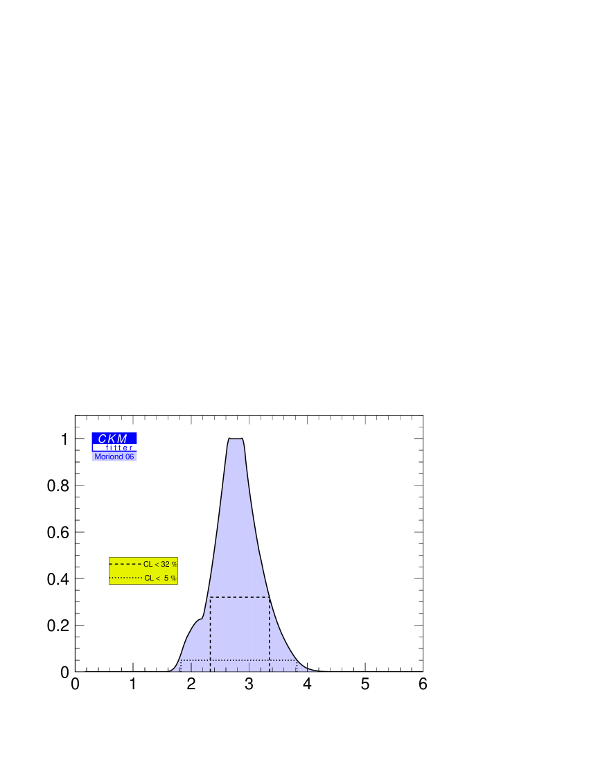
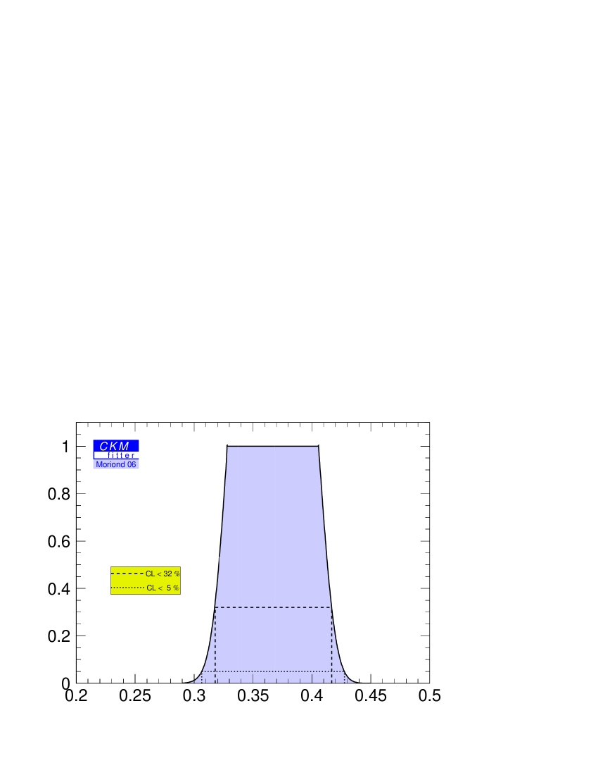
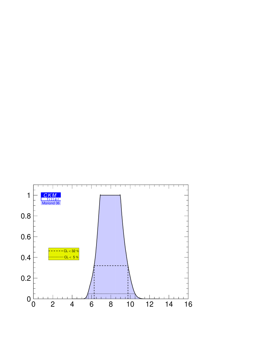
Figure 24: Likelihood of ${\cal B}(K_{L}\to\pi^{0}\nu\bar{\nu})$, $P_{c}(X)$, and ${\cal B}(K^{+}\to\pi^{+}\nu\bar{\nu})$ following from a global CKM analysis performed by the CKMfitter Group ​​. The borders of the $68\%$ ($95\%$) probability regions are indicated by the long (short) dashed lines.

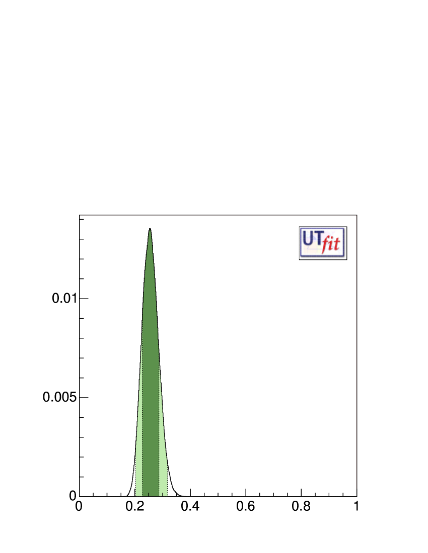
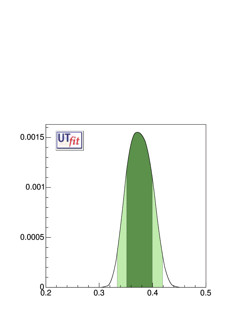
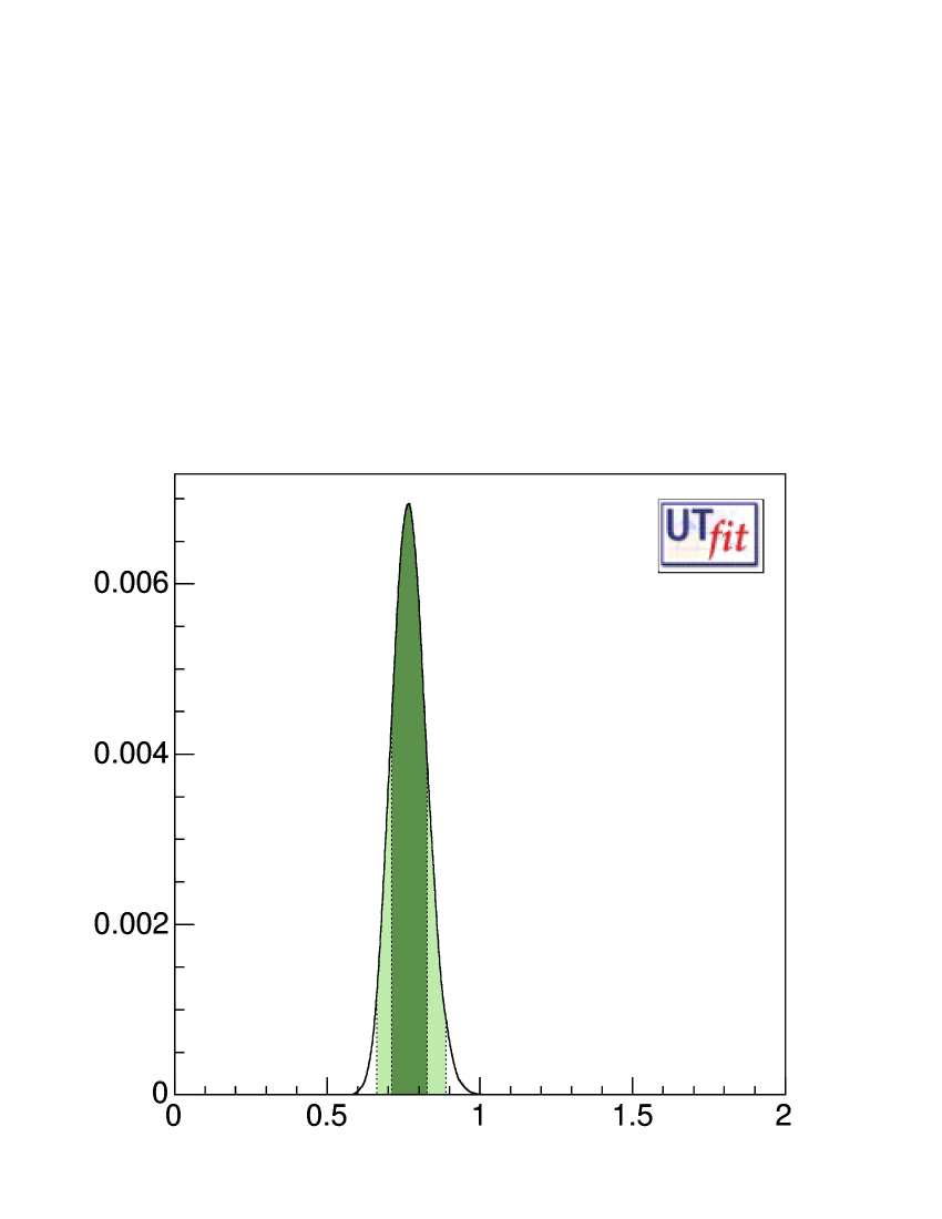
Figure 25: Probability density functions of ${\cal B}(K_{L}\to\pi^{0}\nu\bar{\nu})$, $P_{c}(X)$ and ${\cal B}(K^{+}\to\pi^{+}\nu\bar{\nu})$ following from a global CKM analysis performed by the UTfit Collaboration ​​. Dark (light) areas correspond to the $68\%$ ($95\%$) probability regions.

The numerical results for ${\cal B}(K_{L}\to\pi^{0}\nu\bar{\nu})$, $P_{c}(X)$, and ${\cal B}(K^{+}\to\pi^{+}\nu\bar{\nu})$ obtained by the CKMfitter Group and the UTfit Collaboration are summarized in Tab. 5. The corresponding likelihood and probability density functions are displayed in Figs. 24 and 25. Apart from the CKM elements the employed input agrees with the one that has been used to obtain the numerical values for ${\cal B}(K_{L}\to\pi^{0}\nu\bar{\nu})$, $P_{c}(X)$, and ${\cal B}(K^{+}\to\pi^{+}\nu\bar{\nu})$ presented earlier in Eqs. (118), (119) and (120).

While the CKMfitter Group and the UTfit Collaboration find comparable errors at $95\%$ and higher confidence levels (CL), the UTfit Collaboration obtains significantly smaller errors at the $68\%$ CL. This difference is expected, because both groups treat theoretical errors differently: the UTfit Collaboration assigns a probabilistic meaning to them while the CKMfitter Group scans for a best fit value. It can be most easily understood by discussing the value of $P_{c}(X)$ at NNLO. Here the dominant error is the parametric uncertainty in $m_{c}(m_{c})$, which is treated as a theoretical uncertainty by both groups. By assigning a flat probability density for $m_{c}(m_{c})$ within the error range of $1.25\!{\rm\ GeV}\leq m_{c}(m_{c})\leq 1.35\!{\rm\ GeV}$ only $68\%$ of this measure is used by the UTfit Collaboration to compute $P_{c}(X)$ at the $68\%$ CL. In consequence the error of $P_{c}(X)$ found by the UTfit Collaboration is smaller by a factor of $0.68$ compared to the error one would obtain by treating the uncertainty in $m_{c}(m_{c})$ as the 1$\sigma$ range of a Gaussian distribution. On the other hand the CKMfitter Group uses the whole parameter range of $m_{c}(m_{c})$ to compute the error on $P_{c}(X)$ independently of the CL. For a flat probability density the measure is proportional to the CL such that at the $95\%$ CL nearly the whole range of $m_{c}(m_{c})$ is used by the UTfit Collaboration ​​. Correspondingly the difference in the results for the errors of the CKMfitter Group and the UTfit Collaboration decreases strongly at the $95\%$ and higher CL.

A detailed analysis of the individual sources of uncertainty entering the SM prediction of ${\cal B}(K_{L}\to\pi^{0}\nu\bar{\nu})$ and ${\cal B}(K^{+}\to\pi^{+}\nu\bar{\nu})$ using a modified version of the CKMfitter  package leads to the following picture. In both cases residual scale uncertainties are no longer a dominant source of error as they numerically amount to around $9\%$ and $11\%$ of the total error only. Hence other intrinsic theoretical errors come to fore. In the case of ${\cal B}(K_{L}\to\pi^{0}\nu\bar{\nu})$ the error associated with $r_{K_{L}}$ is now the main source of theoretical uncertainty since the error of these isospin breaking corrections of $\pm 3\%$ translates into around $15\%$ of the total uncertainty. In the case of ${\cal B}(K^{+}\to\pi^{+}\nu\bar{\nu})$ the uncertainties associated with the parameters $\delta P_{c,u}$ and $r_{K^{+}}$ become prominent. Numerically the total error introduced by the long-distance and isospin breaking corrections amounts to about $28\%$ of the final uncertainty in ${\cal B}(K^{+}\to\pi^{+}\nu\bar{\nu})$. This error is thus slightly larger than the error due to the charm quark mass which for $m_{c}(m_{c})=(1.30\pm 0.05)\!{\rm\ GeV}$ amounts to roughly $20\%$ of the final uncertainty. The remaining errors of about $76\%$ and $41\%$ for ${\cal B}(K_{L}\to\pi^{0}\nu\bar{\nu})$ and ${\cal B}(K^{+}\to\pi^{+}\nu\bar{\nu})$, respectively, are due to the uncertainty in the top quark mass, $\alpha_{s}(M_{\scriptscriptstyle Z})$, and the CKM elements. The given numbers have been obtained by removing the individual errors from the fit in the order the have been mentioned in the text. This study makes clear that if one wants to achieve predictions of ${\cal B}(K_{L}\to\pi^{0}\nu\bar{\nu})$ and ${\cal B}(K^{+}\to\pi^{+}\nu\bar{\nu})$ at the level of $\pm 5\%$ or below further theoretical improvements concerning the isospin breaking corrections, long-distance effects, and the determination of the charm quark mass are indispensable.

9.7 Final Predictions for $K_{L}\to\pi^{0}\nu\bar{\nu}$ and $K^{+}\to\pi^{+}\nu\bar{\nu}$

Given the sizeable difference of the $68\%$ CL error intervals obtained by the CKMfitter Group and the UTfit Collaboration we base our final predictions on our own analysis of the charm quark contribution and the branching ratios. To determine our final results for ${\cal B}(K_{L}\to\pi^{0}\nu\bar{\nu})$, $P_{c}(X)$, and ${\cal B}(K^{+}\to\pi^{+}\nu\bar{\nu})$ we could in principle add the errors given in Eqs. (118), (119), and (120) linearly. These estimates might be too conservative. On the other hand adding the errors in quadrature would be probably too optimistic since the uncertainties are not statistically distributed. Therefore we quote as the final result the mean of the values obtained by adding the individual errors once linearly and once in quadrature. In the case of $K_{L}\to\pi^{0}\nu\bar{\nu}$ this gives

$${\cal B}(K_{L}\to\pi^{0}\nu\bar{\nu})=\left(2.8\pm 0.4\right)\times 10^{-11}\,,$$ (121)

while in the case of $K^{+}\to\pi^{+}\nu\bar{\nu}$ one has

$$P_{c}(X)=0.38\pm 0.04\,,$$ (122)

and

$${\cal B}(K^{+}\to\pi^{+}\nu\bar{\nu})=\left(8.0\pm 1.1\right)\times 10^{-11}\,.$$ (123)

The given uncertainties represent the ranges in which we believe that the true values of ${\cal B}(K_{L}\to\pi^{0}\nu\bar{\nu})$, $P_{c}(X)$, and ${\cal B}(K^{+}\to\pi^{+}\nu\bar{\nu})$ are located with high probability.

9.8 Impact on the Determination of the CKM Parameters

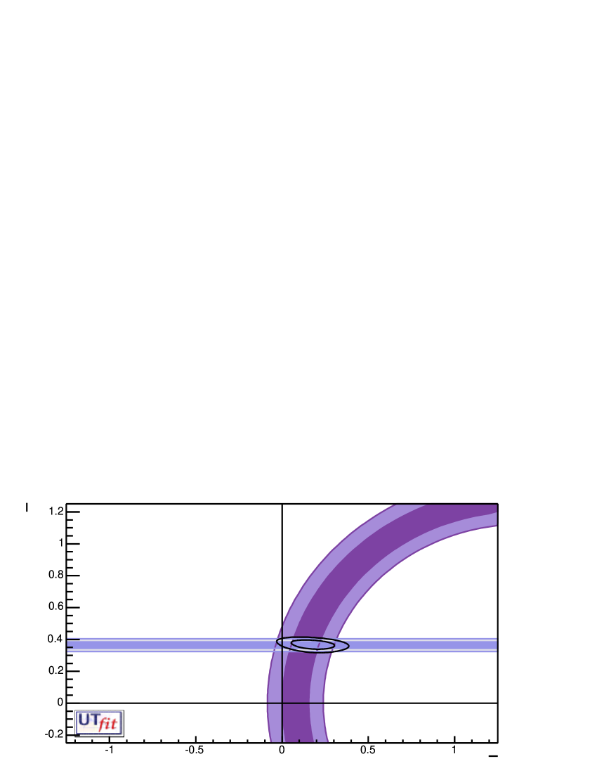
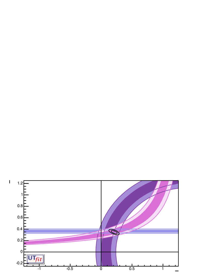
Figure 26: Standard UT from future measurements of ${\cal B}(K_{L}\to\pi^{0}\nu\bar{\nu})$ and ${\cal B}(K^{+}\to\pi^{+}\nu\bar{\nu})$ with an accuracy of $\pm 10\%$. Dark (light) areas correspond to the $68\%$ ($95\%$) probability regions. In the upper (lower) panel the $68\%$ and $95\%$ domains following from the $K\to\pi\nu\bar{\nu}$ constraint (present global CKM fit) as found by the UTfit Collaboration are overlaid. The lower plot also shows for comparison the present constraint coming from $\epsilon_{K}$.

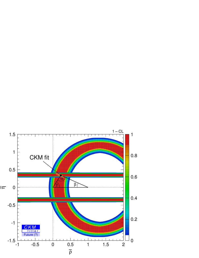
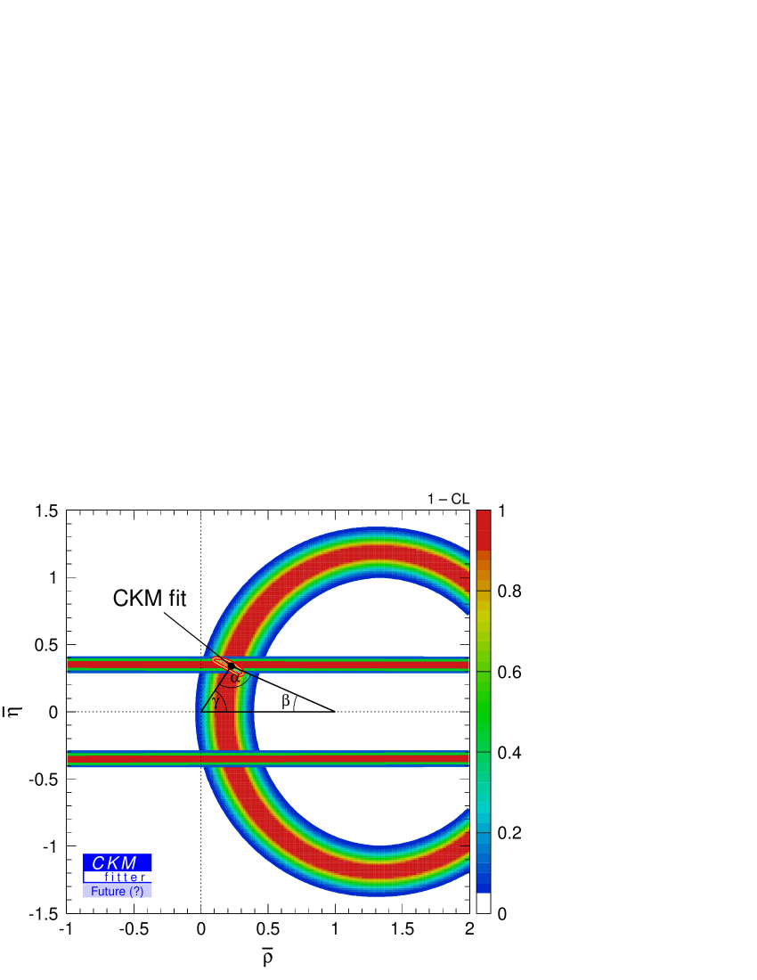
Figure 27: Constraints in the $\bar{\rho}$–$\bar{\eta}$ plane arising from future measurements of ${\cal B}(K_{L}\to\pi^{0}\nu\bar{\nu})$ and ${\cal B}(K^{+}\to\pi^{+}\nu\bar{\nu})$ with an accuracy of $\pm 10\%$. The upper (lower) panel shows the likelihood obtained assuming no (optimistic) improvement of both the theoretical and experimental errors of the input parameters. For comparison the $68\%$ probability region following from the present global CKM analysis of the CKMfitter Group is also displayed.

As seen in Eq. (1) the accuracy of the determination of $|V_{td}|$, $\sin 2\beta$, and of the angle $\gamma$ in the UT depends sensitively on the error in $P_{c}(X)$.

The reduction of the theoretical error in $P_{c}(X)$ from $\pm 9.8\%$ down to $\pm 2.4\%$ translates into the following uncertainties

$$\begin{split}\frac{\sigma\left(|V_{td}|\right)}{|V_{td}|}&=\begin{cases}\pm 4.0\%\,,&\hskip 2.84526pt\text{NLO}\,,\\ \pm 1.0\%\,,&\hskip 2.84526pt\text{NNLO}\,,\end{cases}\\[2.84526pt] \sigma\left(\sin 2\beta\right)&=\begin{cases}\pm 0.024\,,&\text{NLO}\,,\\ \pm 0.006\,,&\text{NNLO}\,,\end{cases}\\[2.84526pt] \sigma\left(\gamma\right)&=\begin{cases}\pm 4.7^{\circ}\,,&\hskip 5.69054pt\text{NLO}\,,\\ \pm 1.2^{\circ}\,,&\hskip 5.69054pt\text{NNLO}\,,\end{cases}\end{split}$$ (124)

implying a very significant improvement of the NNLO over the NLO results. In obtaining these numbers we have used $\sin 2\beta=0.724$ and $\gamma=58.6^{\circ}$ [19], and included only the theoretical errors quoted in Eqs. (3) and (119).

A comparison of $\sin 2\beta$ determined from clean $B$-physics observables with $\sin 2\beta$ inferred from the $K\to\pi\nu\bar{\nu}$ system offers a precise and highly non-trivial test of the CKM picture. Both determinations suffer from small theoretical errors and any discrepancy between them would signal non-CKM physics. The impact of future accurate measurements of $K^{+}\to\pi^{+}\nu\bar{\nu}$ and $K_{L}\to\pi^{0}\nu\bar{\nu}$ leading to ${\cal B}(K^{+}\to\pi^{+}\nu\bar{\nu})=(8.0\pm 0.8)\times 10^{-11}$ and ${\cal B}(K_{L}\to\pi^{0}\nu\bar{\nu})=(3.0\pm 0.3)\times 10^{-11}$ is illustrated in Figs. 27 and 26. As can be seen in Fig. 26 the expected precision of the determination of $(\bar{\rho},\bar{\eta})$ from the $K\to\pi\nu\bar{\nu}$ system cannot quite compete with the one from the present global CKM fit performed by the UTfit Collaboration ​​. On the other hand assuming a reduction of the errors in $M_{t}$, $m_{c}(m_{c})$, $r_{K^{+}}$, $r_{K_{L}}$, and $\delta P_{c,u}$ by a factor of 3 would put the $K\to\pi\nu\bar{\nu}$ system and the global CKM fit almost on the same level. The great potential of the $K\to\pi\nu\bar{\nu}$ system is clearly visible in the lower panel in Fig. 27 which shows the constraint in the $\bar{\rho}$–$\bar{\eta}$ plane obtained by the CKMfitter Group adopting this futuristic scenario.

Obviously, the future of the determination of the standard UT from the $K\to\pi\nu\bar{\nu}$ system will depend on the uncertainties in the measured branching ratios, on the value of $m_{c}(m_{c})$ and also on $|V_{cb}|$. Further theoretical improvement concerning the isospin breaking and long-distance corrections would be desirable in this respect too. A corresponding numerical analysis can be found in the updated version of [3], where the NNLO correction to $P_{c}(X)$ presented here, will be soon included.

While the determination of $|V_{td}|$, $\sin 2\beta$, and $\gamma$ from the $K\to\pi\nu\bar{\nu}$ system is without doubt of interest, with the slow progress in measuring the relevant branching ratios and much faster progress in the determination of the angle $\gamma$ from $B_{s}\to DK$ system to be expected at LHC, the role of the $K\to\pi\nu\bar{\nu}$ system will shift towards the search for new physics rather than the determination of the CKM parameters.

Indeed, determining the CKM parameters from tree diagrams dominated $K$- and $B$-decays and thus independently of new physics contributions will allow to find the “true” values of the CKM parameters and the so-called reference unitarity triangle [62]. Inserting these, hopefully accurate, values in the formulas for the branching ratios presented here, will allow to obtain very precise preditions for the SM rates of both decays. A comparison with future data on these decays will then give a clear signal of potential new physics contributions in a theoretical clean enviroment. Even deviations by $20\%$ from the SM expectations could be considered as signals of new physics, whereas it is not possible in most other decays in which the theoretical uncertainties are at least $10\%$.

10 Summary

In this paper we have calculated the complete NNLO QCD correction of the charm quark contribution to the branching ratio for the rare decay $K^{+}\to\pi^{+}\nu\bar{\nu}$ in the SM. As the charm quark contribution is essentially unaffected by new physics, our results are also valid in basically all extensions of the SM.

The main result of our paper is summarized in the approximate but very accurate analytic expression for the relevant parameter $P_{c}(X)$ as a function of $m_{c}(m_{c})$ and $\alpha_{s}(M_{\scriptscriptstyle Z})$ presented in Eq. (14). The remaining scale uncertainties and the uncertainty due to higher order terms in the computation of $\alpha_{s}(\mu_{c})$ from $\alpha_{s}(M_{\scriptscriptstyle Z})$, that is sizeable at the NLO level as seen in Fig. 23, have been drastically reduced through our calculation to a level that they can basically be ignored for all practical purposes. This can be seen in Tab. 1 and Fig. 23. Nevertheless, an approximate formula for $P_{c}(X)$ containing the dominant parametric and theoretical errors due to $m_{c}(m_{c})$, $\alpha_{s}(M_{\scriptscriptstyle Z})$, $\mu_{c}$, and $\mu_{b}$ has been given in Eq. (115), which should be useful for future phenomenological analysis of the rare decay $K^{+}\to\pi^{+}\nu\bar{\nu}$.

The values of $P_{c}(X)$ for different $m_{c}(m_{c})$ and $\alpha_{s}(M_{\scriptscriptstyle Z})$ are collected in Tab. 2. As $\alpha_{s}(M_{\scriptscriptstyle Z})$ is already known with an accuracy of better than $\pm 2\%$, the main uncertainty in the evaluation of $P_{c}(X)$ resides in the value of $m_{c}(m_{c})$. Our nominal value for $P_{c}(X)=0.38\pm 0.04$ used in the NNLO prediction for the branching ratio of $K^{+}\to\pi^{+}\nu\bar{\nu}$ in Eq. (123) corresponds to $m_{c}(m_{c})=(1.30\pm 0.05)\!{\rm\ GeV}$ but the master formulas for $P_{c}(X)$ in Eqs. (14) and (115) as well as Tab. 2 allow one to calculate $P_{c}(X)$ and ${\cal B}(K^{+}\to\pi^{+}\nu\bar{\nu})$ for other values of $m_{c}(m_{c})$.

With the improved recent evaluation [6] of the long-distance contributions to the charm component, that can be further improved by lattice calculations [7], and hopefully an increased accuracy on $m_{c}(m_{c})$ and $r_{K^{+}}$ in the future, the theoretical computation of the relevant decay rate will reach an exceptional degree of precision, subject mainly to the uncertainties in the values of the CKM parameters. As the latter errors will be reduced to a large extend in the coming years through the $B$-decay experiments a prediction for ${\cal B}(K^{+}\to\pi^{+}\nu\bar{\nu})$ with an accuracy significantly below $\pm 10\%$ will be possible before the end of this decade. Such a precision is unique in the field of FCNC processes.

On the other hand, accurate measurements of ${\cal B}(K^{+}\to\pi^{+}\nu\bar{\nu})$, in particular in conjunction with ${\cal B}(K_{L}\to\pi^{0}\nu\bar{\nu})$, will provide a very important extraction of the CKM parameters that compared with the information from $B$-decays will offer a truly unique test of the CKM mechanism both in the SM and some of its extensions. The drastic reduction of the theoretical uncertainty in $P_{c}(X)$ achieved by the computation presented in this paper will play an important role in these efforts and increases the power of the $K\to\pi\nu\bar{\nu}$ system in the search for new physics, in particular if ${\cal B}(K^{+}\to\pi^{+}\nu\bar{\nu})$ will not differ much from the SM prediction.

Acknowledgments

We are grateful to X. Feng for bringing to our attention the typographical mistakes in Eqs. (108), (111) and (112). We would like to thank Matthias Steinhauser for providing us with an updated version of MATAD [63] and A. Höcker, J. Ocariz, and M. Pierini for useful communications concerning the global analysis of the UT. Discussions with G. Buchalla, S. Jäger, H. Lacker, A. Poschenrieder, F. Schwab, L. Silvestrini, D. Stöckinger, S. Uhlig, and A. Weiler are acknowledged. Finally we are grateful to the CKMfitter Group and the UTfit Collaboration for supplying the numbers and plots shown in Secs. 9.6 and 9.8. This work has been supported in part by the Bundesministerium für Bildung and Forschung under contract 05HT4WOA/3 and the Schweizer Nationalfonds. U. H. and U. N. have been supported by the DOE under contract DE-AC02-76CH03000.

Appendix

A.1 Evanescent Operators

The evanescent operators that arise as counterterms for the one-, two- and three-loop diagrams with insertions of the current-current operators

$$\begin{split}Q^{q}_{1}&=\left(\bar{s}_{\scalebox{0.6}{$L$}}\gamma_{\mu}T^{a}q_{\scalebox{0.6}{$L$}}\right)\left(\bar{q}_{\scalebox{0.6}{$L$}}\gamma^{\mu}T^{a}d_{\scalebox{0.6}{$L$}}\right)\,,\\[2.84526pt] Q^{q}_{2}&=\left(\bar{s}_{\scalebox{0.6}{$L$}}\gamma_{\mu}q_{\scalebox{0.6}{$L$}}\right)\left(\bar{q}_{\scalebox{0.6}{$L$}}\gamma^{\mu}d_{\scalebox{0.6}{$L$}}\right)\,,\end{split}$$ (A.1)

can be chosen to be

$$\begin{split}E^{q}_{1}&=(\bar{s}_{\scalebox{0.6}{$L$}}\gamma_{\mu_{1}\mu_{2}\mu_{3}}T^{a}q_{\scalebox{0.6}{$L$}})(\bar{q}_{\scalebox{0.6}{$L$}}\gamma^{\mu_{1}\mu_{2}\mu_{3}}T^{a}d_{\scalebox{0.6}{$L$}})-\left(16-4\epsilon-4\epsilon^{2}\right)Q^{q}_{1}\,,\\[11.38109pt] E^{q}_{2}&=(\bar{s}_{\scalebox{0.6}{$L$}}\gamma_{\mu_{1}\mu_{2}\mu_{3}}q_{\scalebox{0.6}{$L$}})(\bar{q}_{\scalebox{0.6}{$L$}}\gamma^{\mu_{1}\mu_{2}\mu_{3}}d_{\scalebox{0.6}{$L$}})-\left(16-4\epsilon-4\epsilon^{2}\right)Q^{q}_{2}\,,\\[2.84526pt] E^{q}_{3}&=(\bar{s}_{\scalebox{0.6}{$L$}}\gamma_{\mu_{1}\mu_{2}\mu_{3}\mu_{4}\mu_{5}}T^{a}q_{\scalebox{0.6}{$L$}})(\bar{q}_{\scalebox{0.6}{$L$}}\gamma^{\mu_{1}\mu_{2}\mu_{3}\mu_{4}\mu_{5}}T^{a}d_{\scalebox{0.6}{$L$}})-\left(256-224\epsilon-\frac{5712}{25}\epsilon^{2}\right)Q^{q}_{1}\,,\\ E^{q}_{4}&=(\bar{s}_{\scalebox{0.6}{$L$}}\gamma_{\mu_{1}\mu_{2}\mu_{3}\mu_{4}\mu_{5}}q_{\scalebox{0.6}{$L$}})(\bar{q}_{\scalebox{0.6}{$L$}}\gamma^{\mu_{1}\mu_{2}\mu_{3}\mu_{4}\mu_{5}}d_{\scalebox{0.6}{$L$}})-\left(256-224\epsilon-\frac{10032}{25}\epsilon^{2}\right)Q^{q}_{2}\,,\\[5.69054pt] E^{q}_{5}&=(\bar{s}_{\scalebox{0.6}{$L$}}\gamma_{\mu_{1}\mu_{2}\mu_{3}\mu_{4}\mu_{5}\mu_{6}\mu_{7}}T^{a}q_{\scalebox{0.6}{$L$}})(\bar{q}_{\scalebox{0.6}{$L$}}\gamma^{\mu_{1}\mu_{2}\mu_{3}\mu_{4}\mu_{5}\mu_{6}\mu_{7}}T^{a}d_{\scalebox{0.6}{$L$}})-\left(4096-7680\epsilon\right)Q^{q}_{1}\\[11.38109pt] E^{q}_{6}&=(\bar{s}_{\scalebox{0.6}{$L$}}\gamma_{\mu_{1}\mu_{2}\mu_{3}\mu_{4}\mu_{5}\mu_{6}\mu_{7}}q_{\scalebox{0.6}{$L$}})(\bar{q}_{\scalebox{0.6}{$L$}}\gamma^{\mu_{1}\mu_{2}\mu_{3}\mu_{4}\mu_{5}\mu_{6}\mu_{7}}d_{\scalebox{0.6}{$L$}})-\left(4096-7680\epsilon\right)Q^{q}_{2}\,.\end{split}$$ (A.2)

Here the shorthand notation $\gamma_{\mu_{1}\cdots\mu_{m}}=\gamma_{\mu_{1}}\cdots\gamma_{\mu_{m}}$ and $\gamma^{\mu_{1}\cdots\mu_{m}}=\gamma^{\mu_{1}}\cdots\gamma^{\mu_{m}}$ has been used. The above operators have been defined such that $i)$ the ADM of the operators $Q^{q}_{\pm}$ introduced in Eq. (23) is diagonal through NNLO, and that $ii)$ their particular structure differs only by multiples of $\epsilon^{2}$ times physical operators from the evanescent operators of the “traditional” basis [27, 36]. The latter operators can be found by the procedure outlined in [64]. Up to three loops they have been given in [39]. Of course, the above choice is not unique in the sense, that there are many schemes that would satisfy $i)$ through NNLO. It is however not possible to define the set of evanescent operators to be invariant under the interchange of color structures and to achieve $i)$ simultaneously. Finally, we remark that the $\epsilon^{2}$ terms of the above one-loop evanescent operators $E^{q}_{1}$ and $E^{q}_{2}$ are unambiguously determined by condition $i)$.

In the case of the electroweak box contribution only one evanescent operator arises as a counterterm for the one-, two-, and three-loop diagrams considered in this paper. Following [9, 10, 13] we chose it as

$$E_{\nu}=\frac{m_{c}^{2}}{g^{2}\mu^{2\epsilon}}\sum_{\ell=e,\mu,\tau}(\bar{s}_{\scalebox{0.6}{$L$}}\gamma_{\mu_{1}\mu_{2}\mu_{3}}d_{\scalebox{0.6}{$L$}})(\bar{\nu_{\ell}}_{\scalebox{0.6}{$L$}}\gamma^{\mu_{1}\mu_{2}\mu_{3}}{\nu_{\ell}}_{\scalebox{0.6}{$L$}})-\left(16-4\epsilon\right)Q_{\nu}\,.$$ (A.3)

Here $m_{c}$ is the charm quark $\overline{\rm MS}$ mass $m_{c}(\mu)$ and the explicit factors $g^{-2}$ and $\mu^{-2\epsilon}$ follow from the normalization of $Q_{\nu}$ in Eq. (21).

A.2 Change from the “Standard” Basis of Current-Current Operators

Beyond LO the anomalous dimensions and the Wilson coefficients depend on the definition of the operators in $n=4-2\epsilon$ dimensions. So far all of the direct NNLO calculations have been performed in the operator basis introduced in [38], which we will call “standard” basis from now on. It consists of the following set of physical and evanescent operators

$$\vec{Q^{\prime}}^{T}=(Q^{\prime q}_{1},Q^{\prime q}_{2})\,,\hskip 28.45274pt\vec{E^{\prime}}^{T}=(E^{\prime q}_{1},E^{\prime q}_{2},E^{\prime q}_{3},E^{\prime q}_{4})\,,$$ (A.4)

where

$$\begin{split}Q^{\prime q}_{1}&=\left(\bar{s}_{\scalebox{0.6}{$L$}}\gamma_{\mu}T^{a}q_{\scalebox{0.6}{$L$}}\right)\left(\bar{q}_{\scalebox{0.6}{$L$}}\gamma^{\mu}T^{a}d_{\scalebox{0.6}{$L$}}\right)\,,\\[2.84526pt] Q^{\prime q}_{2}&=\left(\bar{s}_{\scalebox{0.6}{$L$}}\gamma_{\mu}q_{\scalebox{0.6}{$L$}}\right)\left(\bar{q}_{\scalebox{0.6}{$L$}}\gamma^{\mu}d_{\scalebox{0.6}{$L$}}\right)\,,\\[2.84526pt] E^{\prime q}_{1}&=(\bar{s}_{\scalebox{0.6}{$L$}}\gamma_{\mu_{1}\mu_{2}\mu_{3}}T^{a}q_{\scalebox{0.6}{$L$}})(\bar{q}_{\scalebox{0.6}{$L$}}\gamma^{\mu_{1}\mu_{2}\mu_{3}}T^{a}d_{\scalebox{0.6}{$L$}})-16Q^{\prime q}_{1}\\[2.84526pt] E^{\prime q}_{2}&=(\bar{s}_{\scalebox{0.6}{$L$}}\gamma_{\mu_{1}\mu_{2}\mu_{3}}q_{\scalebox{0.6}{$L$}})(\bar{q}_{\scalebox{0.6}{$L$}}\gamma^{\mu_{1}\mu_{2}\mu_{3}}d_{\scalebox{0.6}{$L$}})-16Q^{\prime q}_{2}\,,\\[2.84526pt] E^{\prime q}_{3}&=(\bar{s}_{\scalebox{0.6}{$L$}}\gamma_{\mu_{1}\mu_{2}\mu_{3}\mu_{4}\mu_{5}}T^{a}q_{\scalebox{0.6}{$L$}})(\bar{q}_{\scalebox{0.6}{$L$}}\gamma^{\mu_{1}\mu_{2}\mu_{3}\mu_{4}\mu_{5}}T^{a}d_{\scalebox{0.6}{$L$}})-256Q^{\prime q}_{1}-20E^{\prime q}_{1}\,,\\[2.84526pt] E^{\prime q}_{4}&=(\bar{s}_{\scalebox{0.6}{$L$}}\gamma_{\mu_{1}\mu_{2}\mu_{3}\mu_{4}\mu_{5}}q_{\scalebox{0.6}{$L$}})(\bar{q}_{\scalebox{0.6}{$L$}}\gamma^{\mu_{1}\mu_{2}\mu_{3}\mu_{4}\mu_{5}}d_{\scalebox{0.6}{$L$}})-256Q^{\prime q}_{2}-20E^{\prime q}_{2}\,,\end{split}$$ (A.5)

while

$$\vec{Q}^{T}=(Q^{q}_{+},Q^{q}_{-})\,,\hskip 28.45274pt\vec{E}^{T}=(E^{q}_{1},E^{q}_{2},E^{q}_{3},E^{q}_{4})\,,$$ (A.6)

denotes the physical and evanescent operators used in this paper. The operators $E^{q}_{5}$ and $E^{q}_{6}$ and their primed counterparts have been omitted in the above equations, because they do not affect the change of scheme up to the order considered here.

In this appendix we demonstrate how the results for the two-loop initial conditions [32] and the three-loop ADM [39] of the current-current operators can be transformed to our basis. This will serve as a cross-check of our results for $C^{(k)}_{\pm}(\mu_{\scriptscriptstyle W})$ and $\gamma^{(k)}_{\pm}$ as given in Eqs. (25) and (29). In all formulas presented below we set $C_{\scriptstyle A}=3$ and $C_{\scriptstyle F}=4/3$, while the number of active quark flavors $f$ is kept arbitrary.

The transformations relating the primed with the unprimed sets take the simple form

$$\vec{Q}=\hat{R}\hskip 1.13809pt\vec{Q^{\prime}}\,,\hskip 28.45274pt\vec{E}=\hat{M}\left(\vec{E^{\prime}}+\epsilon\,\hat{U}\vec{Q^{\prime}}+\epsilon^{2}\,\hat{V}\vec{Q^{\prime}}\right)\,,$$ (A.7)

where the matrix $\hat{R}$ ($\hat{M}$) describes a rotation of the physical (evanescent) operators, while the matrix $\hat{U}$ ($\hat{V}$) parameterizes a change of basis that consists of adding multiples of $\epsilon$ ($\epsilon^{2}$) times physical operators to the evanescent ones. The matrices introduced in Eq. (A.7) are given by

$$\begin{split}\hat{R}=\left(\begin{array}[]{cc}1&\frac{2}{3}\\ -1&\frac{1}{3}\end{array}\right),\hskip 28.45274pt\hat{M}=\left(\begin{array}[]{cccc}1&0&0&0\\ 0&1&0&0\\ 20&0&1&0\\ 0&20&0&1\end{array}\right),\\[-5.69054pt] \\[-5.69054pt] \hat{U}=\left(\begin{array}[]{cc}4&0\\ 0&4\\ 144&0\\ 0&144\end{array}\right),\hskip 28.45274pt\hat{V}=\left(\begin{array}[]{cccc}4&0\\ 0&4\\ \frac{3712}{25}&0\\ 0&\frac{8032}{75}\end{array}\right).\end{split}$$ (A.8)

The change of basis in Eq. (A.7) is $\mu$-independent and leaves, apart from a global rotation, the anomalous dimensions and the Wilson coefficients invariant. It, however, induces a finite renormalization of the physical operators. In order to restore the standard $\overline{\rm MS}$ renormalization conditions these contributions must be removed by a change of scheme. Hence a $\epsilon$-dependent linear transformation of the operator basis is equivalent to a global rotation and a change of scheme [39].

The finite renormalization corresponding to the above change of basis can be derived with simple algebra. Through ${\cal O}(\alpha_{s}^{2})$ we find

$$\begin{split}\hat{Z}^{(1,0)}_{QQ}&=-\hat{R}\hskip 1.13809pt\hat{Z}^{\prime(1,1)}_{QE}\hat{U}\hat{R}^{-1}\,,\\[2.84526pt] \hat{Z}^{(2,0)}_{QQ}&=-\hat{R}\left(\hat{Z}^{\prime(2,1)}_{QE}\hat{U}+\hat{Z}^{\prime(2,2)}_{QE}\hat{V}-\frac{1}{2}\hat{Z}^{\prime(1,1)}_{QE}\hat{V}\hat{\gamma}^{\prime(0)}\right)\hat{R}^{-1}\,,\end{split}$$ (A.9)

where

$$\hat{Z}^{\prime(2,2)}_{QE}=\frac{1}{2}\left(\hat{Z}^{\prime(1,1)}_{QE}\hat{Z}^{\prime(1,1)}_{EE}+\frac{1}{2}\hat{\gamma}^{\prime(0)}\hat{Z}^{\prime(1,1)}_{QE}-\beta_{0}\hat{Z}^{\prime(1,1)}_{QE}\right)\,.$$ (A.10)

As always, the matrix $\hat{M}$ encoding the rotation of evanescent operators does not affect the residual finite renormalization. Eqs. (A.9) and (A.10) agree with the NLO formulas of [29, 38] and generalize the NNLO formulas of [39].

The only feature which has not been discussed in the literature before is the appearance of the $\epsilon^{2}$-dependent transformation characterized by $\hat{V}$ in Eq. (A.7). It induces a finite ${\cal O}(\alpha_{s}^{2})$ renormalization described by the second and third term in the second line of Eqs. (A.9). The former term is analogous to the first line of Eqs. (A.9). The latter term stems from a $\epsilon$-dependent ${\cal O}(\alpha_{s})$ renormalization. While the $\epsilon$-dependent change of scheme removes the finite terms, it still leaves the anomalous dimensions and the Wilson coefficients invariant. Yet it induces a finite ${\cal O}(\alpha_{s}^{2})$ renormalization. The transformation to the standard $\overline{\rm MS}$ scheme definitions requires the removal of this finite term, which is achieved by the last term in the second line of Eqs. (A.9).

The matrices entering the above equations are found from one- and two-loop matrix elements of physical and evanescent operators in the “standard” basis. The ${\cal O}(\alpha_{s})$ ADM takes the following form [38, 39, 42]

$$\hat{\gamma}^{\prime(0)}=\left(\begin{array}[]{cc}-4&\frac{8}{3}\\ 12&0\end{array}\right)\,.$$ (A.11)

For the ${\cal O}(\alpha_{s})$ mixing into the evanescent operators one obtains [38, 39, 42]

$$\hat{Z}^{\prime(1,1)}_{QE}=\left(\begin{array}[]{cccc}\frac{5}{12}&\frac{2}{9}&0&0\\ 1&0&0&0\end{array}\right)\,,\hskip 28.45274pt\hat{Z}^{\prime(1,1)}_{EE}=\left(\begin{array}[]{cccc}-7&-\frac{4}{3}&\frac{5}{12}&\frac{2}{9}\\ -6&0&1&0\\ 0&0&\frac{13}{3}&-\frac{28}{9}\\ 0&0&-14&-\frac{64}{3}\end{array}\right)\,.$$ (A.12)

At ${\cal O}(\alpha_{s}^{2})$ only the mixing of physical into evanescent operators is needed. It is given by [39, 42]

$$\hat{Z}^{(2,1)}_{QE}=\left(\begin{array}[]{cccc}\frac{1531}{288}-\frac{5}{216}f&-\frac{1}{72}-\frac{1}{81}f&\frac{1}{384}&-\frac{35}{864}\\ \frac{119}{16}-\frac{1}{18}f&\frac{8}{9}&-\frac{35}{192}&-\frac{7}{72}\end{array}\right)\,.$$ (A.13)

The general NNLO formulas relating the initial conditions of the Wilson coefficients and the ADM in two different schemes have been derived recently [39]. They read

$$\vec{C}(\mu_{\scriptscriptstyle W})=\left(\hat{1}+\frac{\alpha_{s}(\mu_{\scriptscriptstyle W})}{4\pi}\hat{Z}^{(1,0)}_{QQ}+\left(\frac{\alpha_{s}(\mu_{\scriptscriptstyle W})}{4\pi}\right)^{2}\hat{Z}^{(2,0)}_{QQ}\right)^{T}\!\!(\hat{R}^{-1}\big{)}^{T}\vec{C}^{\prime}(\mu_{\scriptscriptstyle W})\,,$$ (A.14)

and

$$\begin{split}\hat{\gamma}^{(0)}&=\hat{R}\hskip 0.56905pt\hat{\gamma}^{\prime(0)}\hskip 0.56905pt\hat{R}^{-1}\,,\\[8.53581pt] \hat{\gamma}^{(1)}&=\hat{R}\hskip 0.56905pt\hat{\gamma}^{\prime(1)}\hskip 0.56905pt\hat{R}^{-1}-\left[\hat{Z}^{(1,0)}_{QQ},\hat{\gamma}^{(0)}\right]-2\beta_{0}\hat{Z}^{(1,0)}_{QQ}\,,\\[5.69054pt] \hat{\gamma}^{(2)}&=\hat{R}\hat{\gamma}^{\prime(2)}\hat{R}^{-1}-\left[\hat{Z}^{(2,0)}_{QQ},\hat{\gamma}^{(0)}\right]-\left[\hat{Z}^{(1,0)}_{QQ},\hat{\gamma}^{(1)}\right]-\left[\hat{Z}^{(1,0)}_{QQ},\hat{\gamma}^{(0)}\right]\hat{Z}^{(1,0)}_{QQ}\\[2.84526pt] &-4\beta_{0}\hat{Z}^{(2,0)}_{QQ}-2\beta_{1}\hat{Z}^{(1,0)}_{QQ}+2\beta_{0}\big{(}\hat{Z}^{(1,0)}_{QQ}\big{)}^{2}\,.\end{split}$$ (A.15)

Eqs. (A.8) to (A.15) allow one to transform the results for the initial conditions of the Wilson coefficients of the current-current operators and their ADM in the “standard” basis to the basis used in this paper. This enables us to verify that the well-established NLO results [38, 39, 42] coincide, after the change of scheme, with the expressions presented in the second line of Eqs. (25) and (29). For what concerns the NNLO we confirm both the two-loop initial conditions of the Wilson coefficients [32] as well as the corresponding three-loop ADM [39].

Erratum

Abstract

We correct the treatment of anomalous triangle diagrams occuring in the effective theory in which the heavy top quark is integrated out. To this end we determine the initial conditions and anomalous dimensions of the operator describing the $Z$-mediated coupling of neutrinos to quarks and further rectify the bilocal renormalization group evolution. Our changes affect the charm-quark contribution $P_{c}(X)$ at the next-to-leading and next-to-next-to-leading orders, but are numerically negligible as they amount to relative shifts below a permille.

$Z$ Penguin

Contrary to the statements in Sec. 6.1 the diagrams in Fig. 9 vanish for $m_{t}\to\infty$. As a consequence, the Wilson coefficient of the Chern-Simons operator $Q_{CS}$ also vanishes and the anomalous diagrams will not drop out in a next-to-leading (NLO) and next-to-next-to-leading order (NNLO) calculation of the charm-quark contribution to $K\to\pi^{+}\nu\bar{\nu}$. There is no more reason to include $Q_{CS}$ in the definition of $Q_{Z}$ in Eq. (37). Further the Wilson coefficients of $Q_{V}^{q}$ and $Q_{A}^{q}$ are different, so that the definition of $Q_{Z}$ is not helpful for the description of the anomalous effects. To maintain the canonical normalization of the coefficients we define

$$Q_{Z}^{q}=-I^{3}_{q}Q_{A}^{q}\,$$ (E.1)

recalling that $I^{3}_{q}=\pm 1/2$ denotes the third component of the weak isospin. Since complete isospin doublets do not contribute to the anomalous triangle diagram, it is sufficient to consider diagrams with a bottom-quark loop stemming from matrix elements involving $Q_{Z}^{b}$. A useful operator basis is $(Q_{Z}^{b},Q_{Z}^{\rm sg},Q_{Z}^{\rm nsg})$ with the flavor-singlet and flavor-non-singlet operators

$$\begin{split}Q_{Z}^{\rm sg}&=Q_{Z}^{s}+Q_{Z}^{d}-Q_{Z}^{c}-Q_{Z}^{u}\\ &=\frac{1}{2}\sum_{\ell=e,\mu,\tau}\left[\overline{s}\gamma_{\mu}\gamma_{5}s+\overline{d}\gamma_{\mu}\gamma_{5}d+\overline{c}\gamma_{\mu}\gamma_{5}c+\overline{u}\gamma_{\mu}\gamma_{5}u\right]\,\overline{\nu}{}_{\ell L}\gamma^{\mu}\nu_{\ell L}\,,\\[5.69054pt] Q_{Z}^{\rm nsg}&=Q_{Z}^{s}+Q_{Z}^{d}+Q_{Z}^{c}+Q_{Z}^{u}\\ &=\frac{1}{2}\sum_{\ell=e,\mu,\tau}\left[\overline{s}\gamma_{\mu}\gamma_{5}s+\overline{d}\gamma_{\mu}\gamma_{5}d-\overline{c}\gamma_{\mu}\gamma_{5}c-\overline{u}\gamma_{\mu}\gamma_{5}u\right]\,\overline{\nu}{}_{\ell L}\gamma^{\mu}\nu_{\ell L}\,.\end{split}$$ (E.2)

The operator $Q_{Z}^{\rm nsg}$ does not participate in the renormalization group (RG) evolution and its coefficient satisfies $C_{Z}^{\rm nsg}(\mu)=1$ at all scales $\mu_{c}\leq\mu\leq\mu_{\scriptscriptstyle W}$. The coefficients $C_{Z}^{b}$ and $C_{Z}^{\rm sg}$ have non-trivial initial conditions at the scale $\mu_{\scriptscriptstyle W}$, at which the top quark is integrated out, and further run for $\mu_{b}\leq\mu\leq\mu_{\scriptscriptstyle W}$, with their RG evolution determined by the anomalous dimension $\gamma_{A}$ calculated from the renormalization factor $Z_{AA}$ defined in Eqs. (52). In our paper we consider different renormalization schemes for $\gamma_{5}$: in $Q_{Z}^{b}$ we use the ’t Hooft-Veltman (HV) scheme, which amounts to the replacement of $\overline{b}\gamma^{\mu}\gamma_{5}b$ by $-(i/3!)\,\epsilon^{\mu_{1}\mu_{2}\mu_{3}\mu}\,\overline{b}\gamma_{\mu_{1}}\gamma_{\mu_{2}}\gamma_{\mu_{3}}b$ [17]. The diagrams for the NLO and NNLO anomalous dimension describe the mixing of $Q_{Z}^{b}$ into $Q_{Z}^{\rm sg}$ and the diagrams of the bilocal mixing discussed in Sec. 3 involve $Q_{Z}^{\rm sg}$ with open quark lines only, so that the definition of the naive dimensional regularization (NDR) scheme is unambigous here. We perform these calculation in two schemes, choosing either HV or NDR for the open quark line. At NNLO, the initial condition of the Wilson coefficient $C_{Z}^{q}$ is the same in HV and NDR:

$$C_{Z}^{q}(\mu_{\scriptscriptstyle W})=1\,+\,\left(\frac{\alpha_{s}(\mu_{\scriptscriptstyle W})}{4\pi}\right)^{2}C_{Z}^{q\,(2)}(\mu_{\scriptscriptstyle W})\,,\qquad\mbox{with}\quad C_{Z}^{q\,(2)}(\mu_{\scriptscriptstyle W})=2I_{q}^{3}\,6C_{F}\ln\frac{m_{t}^{2}}{\mu_{\scriptscriptstyle W}^{2}}\,,$$ (E.3)

and $C_{F}=4/3$. It follows that

$$C_{Z}^{\rm sg}(\mu_{\scriptscriptstyle W})=\left(\frac{\alpha_{s}(\mu_{\scriptscriptstyle W})}{4\pi}\right)^{2}C_{Z}^{b\,(2)}(\mu_{\scriptscriptstyle W}).$$ (E.4)

The results in Eqs. (E.3) and (E.4) assume that the same scheme for $\gamma_{5}$ is used in the full standard model (SM) and the effective five-quark theory. $C_{Z}^{q}(\mu_{\scriptscriptstyle W})$ is calculated from the two-loop diagram obtained by attaching a quark line to the two gluons to the left diagram in Fig. 9 and a second diagram with reversed orientation of the quark loop. The finite renormalization constant $Z_{AA}^{(2,0)}$ defined in Eq. (55) is taken into account here. The leading order (LO) $2\times 2$ anomalous dimension matrix (ADM) $\hat{\gamma}_{Z}^{(0)}$ for $(Q_{Z}^{b},Q_{Z}^{\rm sg})$ vanishes. For the NLO and NNLO ADM we find

$$\hat{\gamma}_{Z}^{(n)}=\begin{pmatrix}\gamma_{A}^{(n)}&\gamma_{A}^{(n)}\\ 4\gamma_{A}^{(n)}&4\gamma_{A}^{(n)}\end{pmatrix}\,,\qquad n=1,2\,,$$ (E.5)

in the HV scheme, confirming the anomalous dimensions of the axial current calculated in [17]:

$$\gamma_{A}^{(1)}=12C_{F}\,,\qquad\gamma_{A}^{(2)}=\frac{284}{3}C_{F}C_{A}-\frac{8}{3}C_{F}f-36C_{F}^{2}\,.$$ (E.6)

Here $C_{A}=3$ and $f$ denotes the number of active quark flavors. A priori the element $\big{(}\hat{\gamma}_{Z}^{(n)}\big{)}_{12}$ may depend on the choice of the scheme for $Q_{Z}^{\rm sg}$: the HV scheme involves a finite one-loop counterterm [17] to remove a spurious anomaly from diagrams with an open quark line. This finite counterterm is absent in the NDR scheme, which instead involves a finite counterterm to the evanescent operator $E_{A}^{q}$ defined in Eq. (53). We find that the analytical results for $\big{(}\hat{\gamma}_{Z}^{(1)}\big{)}_{12}$ and $\big{(}\hat{\gamma}_{Z}^{(2)}\big{)}_{12}$ are the same in both schemes.

The Wilson coefficients $\vec{C}_{Z}=(C_{Z}^{b},C_{Z}^{\rm sg})^{T}$ for $\mu_{b}\leq\mu<\mu_{\scriptscriptstyle W}$ are obtained in the usual way by solving

$$\mu\frac{d}{d\mu}\vec{C}(\mu)=\hat{\gamma}_{Z}^{T}\vec{C}(\mu).$$ (E.7)

At the scale $\mu_{b}$ the bottom quark is integrated out and we have to match the five-flavor and four-flavor theories. The corresponding Hamiltonians are

$${\cal H}_{\rm eff}^{f=5,Z} =\frac{\pi\alpha}{M_{\scriptscriptstyle W}^{2}\sin^{2}\theta_{\scriptscriptstyle W}}\left[C_{Z}^{b}Q_{Z}^{b}+C_{Z}^{\rm nsg}Q_{Z}^{\rm nsg}+C_{Z}^{5,{\rm sg}}Q_{Z}^{\rm sg}\right],$$

$${\cal H}_{\rm eff}^{f=4,Z} =\frac{\pi\alpha}{M_{\scriptscriptstyle W}^{2}\sin^{2}\theta_{\scriptscriptstyle W}}\left[C_{Z}^{\rm nsg}Q_{Z}^{\rm nsg}+C_{Z}^{4,{\rm sg}}Q_{Z}^{\rm sg}\right]$$

with $C_{Z}^{f,{\rm nsg}}=1$ in both theories. From the two-loop triangle diagrams with bottom quark one finds:

$$\begin{split}C_{Z}^{4,{\rm sg}}(\mu_{b})&=C_{Z}^{5,{\rm sg}}(\mu_{b})+C_{Z}^{b}(\mu_{b})\left(\frac{\alpha_{s}(\mu_{b})}{4\pi}\right)^{2}6C_{F}\ln\frac{m_{b}^{2}}{\mu_{b}^{2}}\\ &=C_{Z}^{5,{\rm sg}}(\mu_{b})+\left(\frac{\alpha_{s}(\mu_{b})}{4\pi}\right)^{2}6C_{F}\ln\frac{m_{b}^{2}}{\mu_{b}^{2}}+{\cal O}\left(\alpha_{s}^{4}\right).\end{split}$$ (E.8)

Inserting Eqs. (E.3) to (E.5) into the NNLO RG evolution equation [39] entails:

$$\begin{split}C_{Z}^{5,{\rm sg}}(\mu_{b})&=\frac{\gamma_{A}^{(1)}}{2\beta_{0}}\frac{\alpha_{s}(\mu_{\scriptscriptstyle W})-\alpha_{s}(\mu_{b})}{4\pi}+\frac{5}{8}\frac{\big{(}\gamma_{A}^{(1)}\big{)}^{2}}{\beta_{0}^{2}}\left(\frac{\alpha_{s}(\mu_{\scriptscriptstyle W})-\alpha_{s}(\mu_{b})}{4\pi}\right)^{2}\\ &\phantom{xx}-\frac{\beta_{0}\gamma_{A}^{(2)}-\beta_{1}\gamma_{A}^{(1)}}{4\beta_{0}^{2}}\frac{\alpha_{s}^{2}(\mu_{\scriptscriptstyle W})-\alpha_{s}^{2}(\mu_{b})}{(4\pi)^{2}}+\left(\frac{\alpha_{s}(\mu_{\scriptscriptstyle W})}{4\pi}\right)^{2}C_{Z}^{b\,(2)}(\mu_{\scriptscriptstyle W})\,,\\[5.69054pt] C_{Z}^{5,b}(\mu_{b})&=1+C_{Z}^{5,{\rm sg}}(\mu_{b})\,.\end{split}$$ (E.9)

Numerically, we find

$$C_{Z}^{\rm sg}(m_{b})=-0.011\,,$$ (E.10)

with negligible variation when $\mu_{\scriptscriptstyle W}$ is changed between $M_{\scriptscriptstyle W}$ and $m_{t}$ or if $m_{b}$, $m_{t}$, or $\alpha_{s}(M_{\scriptscriptstyle Z})$ are varied within their experimental errors.

Bilocal Evolution

In order to determine the charm-quark contribution of $K^{+}\to\pi^{+}\nu\overline{\nu}$ we need the bilocal mixings of $(C_{Z}^{c},C_{\pm})$ and $(C_{Z}^{b},C_{\pm})$ into the coefficient $C_{\nu}$. The relevant three-loop anomalous dimension

$$\gamma^{A\Delta(2)}_{\pm,\,\nu}=6Z^{\Delta(3,1)}_{\pm A,\,\nu}-4Z^{(2,1)}_{AE}Z^{P(1,0)}_{\pm E,\,\nu}-4Z^{\Delta(2,0)}_{AA}Z^{P(1,1)}_{\pm A,\,\nu}$$ (E.11)

can be inferred from Eqs. (54), (55), (62) and (63). In the NDR scheme we obtain:

$$\gamma^{A\Delta(2)}_{\pm,\,\nu}=12C_{F}(1\pm 5C_{A})\,.$$ (E.12)

We write the Wilson coefficient for the $Z$-penguin contribution to $C_{\nu}$ as $C_{\nu}^{P}+C_{\nu}^{\Delta}$. Here $C_{\nu}^{P}$ is the piece coming from the non-anomalous diagrams obtained by solving the RG equation in (47), with the solution quoted in Eq. (86). $C_{\nu}^{\Delta}$ is the new contribution from the triangle diagrams. The RG equation read

$$\mu\frac{d}{d\mu}\left[C_{\nu}^{P}(\mu)+C_{\nu}^{\Delta}(\mu)\right]=\gamma_{\nu}\left[C_{\nu}^{P}(\mu)+C_{\nu}^{\Delta}(\mu)\right]+\,\,4\!\!\!\!\!\sum_{\begin{subarray}{c}i=\pm\\ j=b,{\rm nsg,sg}\end{subarray}}\gamma_{ij,\,\nu}C_{i}(\mu)C_{Z}^{j}(\mu)\,.$$ (E.13)

From the definition of $Q_{b,\rm nsg,sg}$ we find

$$\gamma_{\pm\,b,\,\nu}=\tfrac{1}{2}\gamma^{A\Delta}_{\pm,\,\nu}\,,\qquad\quad\gamma_{\pm\,{\rm nsg},\,\nu}=\gamma^{P}_{\pm,\,\nu}=-\tfrac{1}{2}\gamma^{A}_{\pm,\,\nu}\,,\qquad\quad\gamma_{\pm\,{\rm sg},\,\nu}=\tfrac{1}{2}\gamma^{A}_{\pm,\,\nu}+\tfrac{1}{2}\gamma^{A\Delta}_{\pm,\,\nu}\,.$$ (E.14)

The expressions for $\gamma^{A}_{\pm,\,\nu}$, calculated from the non-anomalous diagrams, are listed in Eq. (51). Subtracting the RGE for $C_{\nu}^{P}(\mu)$ in Eq. (47) from (E.14) we find:

$$\mu\frac{d}{d\mu}C_{\nu}^{\Delta}(\mu)=\gamma_{\nu}C_{\nu}^{\Delta}(\mu)+2\sum_{i=\pm}\left[\gamma^{A\Delta}_{i,\,\nu}C_{i}(\mu)C_{Z}^{b}(\mu)+\left(\gamma^{A\Delta}_{i,\,\nu}+\gamma^{A}_{i,\,\nu}\right)C_{i}(\mu)C_{Z}^{\rm sg}(\mu)\right]\,.$$ (E.15)

This RG equation splits into two linear differential equations which are easily solved, as discussed for example in [65] for an analogous case.

Figure 28: $\Delta P_{c}(X)$ as a function of the renormalization scale $\mu_{c}$. The dashed (solid) line represents the NLO (NNLO) result.

To NNLO only the one-loop matrix elements involving a double operator insertion $(Q_{\pm}^{q},Q_{Z}^{\rm sg})$ gives a non-trivial contribution to the matching at $\mu_{c}$. We write the contribution to the tree-level matrix element $\langle Q_{\nu}\rangle^{(0)}$ in the following way

$$\left\langle Q_{\pm}^{\rm sg}(\mu_{c})\right\rangle=\frac{\alpha_{s}(\mu_{c})}{4\pi}r^{{\rm sg}\,(1)}_{\pm}(\mu_{c})\langle Q_{\nu}\rangle^{(0)}=-\frac{\alpha_{s}(\mu_{c})}{4\pi}r^{P\,(1)}_{\pm}(\mu_{c})\langle Q_{\nu}\rangle^{(0)}\,,$$ (E.16)

where $r^{P\,(1)}_{\pm}(\mu_{c})$ codifies the one-loop corrections detailed in Eqs. (83) and (84) and $Q_{\pm}^{\rm sg}$ is defined analogously to $Q_{\pm}^{P}$ in Eq. (19).

We have now collected all ingredients necessary to determine the missing contribution $\Delta P_{c}(X)$ to the charm-quark contribution in $K^{+}\to\pi^{+}\nu\bar{\nu}$, represented by the parameter $P_{c}(X)$ defined in Eq. (13) of the paper. For the NLO and NNLO coefficient in the perturbative expansion

$$\Delta P_{c}(X)=\Delta P_{c}^{(1)}(X)+\frac{\alpha_{s}(\mu_{c})}{4\pi}\Delta P_{c}^{(2)}(X)\,,$$ (E.17)

we plot the $\mu_{c}$-dependence in Fig. 28. The charm-quark corrections due to anomalous triangle graphs lead to shifts in $P_{c}(X)$ in the ballpark of $-0.0001$ with the exact value depending on the renormalization scale. Recalling that $P_{c}(X)=0.369$ ($P_{c}(X)=0.375$) at NLO (NNLO) the corresponding relative shift amounts to $-0.05\%$ ($-0.01\%$). One can understand the smallness of the NLO contribution to $\Delta P_{c}(X)$ by inspecting the logarithmic expansion of our result: the NLO term starts only at $\mathcal{O}(\alpha_{s}^{2}\hskip 0.7113pt\ln(\mu_{\scriptscriptstyle W}^{2}/\mu_{b}^{2})\hskip 0.7113pt\ln(\mu_{\scriptscriptstyle W}^{2}/\mu_{c}^{2}))$, which is of the same order in $\alpha_{s}$ as the NNLO correction containing only one large logarithm. Expanding $\Delta P_{c}(X)$ in $\alpha_{s}$ we find explicitly

$$\Delta P_{c}(X)=\frac{1}{\lambda^{4}}\frac{m_{c}^{2}}{M_{\scriptscriptstyle W}^{2}}\left(\frac{\alpha_{s}}{4\pi}\right)^{2}\left\{\left(\ln\frac{\mu_{\scriptscriptstyle W}^{2}}{\mu_{b}^{2}}-2\ln\frac{\mu_{\scriptscriptstyle W}^{2}}{\mu_{c}^{2}}+1\right)\ln\frac{\mu_{\scriptscriptstyle W}^{2}}{\mu_{b}^{2}}\right\}+\mathcal{O}\Big{(}\alpha_{s}^{2}\ln^{0}\frac{\mu_{\scriptscriptstyle W}^{2}}{\mu_{b}^{2}},\alpha_{s}^{3}\Big{)}\,,$$ (E.18)

where the $\alpha_{s}^{2}$ suppression is accompanied by terms with small numerical coefficients of opposite sign. Notice that the exact result $\Delta P_{c}(X)$ is smaller by two orders of magnitude than the total NNLO uncertainty in $P_{c}(X)$ of $\pm 0.015$. In view of these numbers it is clear that our erroneous treatment of anomalous triangle diagrams has no phenomenological impact.

Acknowledgements

We are grateful to Konstantin Chetyrkin and Mikolaj Misiak for pointing our mistake out to us. We also thank Johann Kühn for bringing the article [66], in which the large logarithm occuring from the anomalous triangle diagrams has been discovered, to our attention. We further thank Mikolaj Misiak and Gerhard Buchalla for a thorough proofreading and comments on this erratum.

References

- [1] G. Buchalla and A. J. Buras, Phys. Lett. B 333, 221 (1994) [arXiv:hep-ph/9405259] and Phys. Rev. D 54, 6782 (1996) [arXiv:hep-ph/9607447].
- [2] G. Isidori, Annales Henri Poincare 4, S97 (2003) [arXiv:hep-ph/0301159]; in Proceedings of the 2nd Workshop on the CKM Unitarity Triangle, Durham, England, 2003, eConf C0304052, WG304 (2003) [arXiv:hep-ph/0307014] and references therein.
- [3] A. J. Buras, F. Schwab and S. Uhlig, arXiv:hep-ph/0405132.
- [4] W. J. Marciano and Z. Parsa, Phys. Rev. D 53, 1 (1996).
- [5] G. Ecker, A. Pich and E. de Rafael, Nucl. Phys. B 303, 665 (1988); D. Rein and L. M. Sehgal, Phys. Rev. D 39, 3325 (1989); J. S. Hagelin and L. S. Littenberg, Prog. Part. Nucl. Phys. 23, 1 (1989); M. Lu and M. B. Wise, Phys. Lett. B 324, 461 (1994) [arXiv:hep-ph/9401204]; C. Q. Geng, I. J. Hsu and Y. C. Lin, Phys. Rev. D 50, 5744 (1994) [arXiv:hep-ph/9406313] and Phys. Lett. B 355, 569 (1995) [arXiv:hep-ph/9506313]; S. Fajfer, Nuovo Cim. A 110, 397 (1997) [arXiv:hep-ph/9602322]; A. F. Falk, A. Lewandowski and A. A. Petrov, Phys. Lett. B 505, 107 (2001) [arXiv:hep-ph/0012099].
- [6] G. Isidori, F. Mescia and C. Smith, Nucl. Phys. B 718, 319 (2005) [arXiv:hep-ph/0503107].
- [7] G. Isidori, G. Martinelli and P. Turchetti, arXiv:hep-lat/0506026.
- [8] N. Cabibbo, Phys. Rev. Lett. 10, 531 (1963); M. Kobayashi and T. Maskawa, Prog. Theor. Phys. 49, 652 (1973).
- [9] G. Buchalla and A. J. Buras, Nucl. Phys. B 412, 106 (1994) [arXiv:hep-ph/9308272].
- [10] G. Buchalla and A. J. Buras, Nucl. Phys. B 548, 309 (1999) [arXiv:hep-ph/9901288].
- [11] W. A. Bardeen, A. J. Buras, D. W. Duke and T. Muta, Phys. Rev. D 18, 3998 (1978).
- [12] G. Buchalla and A. J. Buras, Nucl. Phys. B 398, 285 (1993) and B 400, 225 (1993).
- [13] M. Misiak and J. Urban, Phys. Lett. B 451, 161 (1999) [arXiv:hep-ph/9901278].
- [14] A. I. Vainshtein, V. I. Zakharov, V. A. Novikov and M. A. Shifman, Phys. Rev. D 16, 223 (1977); J. R. Ellis and J. S. Hagelin, Nucl. Phys. B 217, 189 (1983); C. Dib, I. Dunietz and F. J. Gilman, Mod. Phys. Lett. A 6, 3573 (1991).
- [15] A. J. Buras, M. Gorbahn, U. Haisch and U. Nierste, Phys. Rev. Lett. 95, 261805 (2005) [arXiv:hep-ph/0508165].
- [16] S. S. Chern and J. Simons, Annals Math. 99, 48 (1974).
- [17] S. A. Larin, Phys. Lett. B 303, 113 (1993) [arXiv:hep-ph/9302240].
- [18] S. L. Adler, Phys. Rev. 177, 2426 (1969); J. S. Bell and R. Jackiw, Nuovo Cim. A 60, 47 (1969).
- [19] J. Charles et al. [CKMfitter Group], Eur. Phys. J. C 41, 1 (2005), [arXiv:hep-ph/0406184] and August 1, 2005 update available at http://www.slac.stanford.edu/ xorg/ckmfitter/ckm_results_summerEPS2005.html.
- [20] M. Ciuchini et al., JHEP 0107, 013 (2001) [arXiv:hep-ph/0012308] and September 22, 2005 update available at http://utfit.roma1.infn.it/.
- [21] J. F. Arguin et al. [The Tevatron Electroweak Working Group], arXiv:hep-ex/0507091.
- [22] C. Bobeth, P. Gambino, M. Gorbahn and U. Haisch, JHEP 0404, 071 (2004) [arXiv:hep-ph/0312090].
- [23] G. Buchalla and A. J. Buras, Phys. Rev. D 57, 216 (1998) [arXiv:hep-ph/9707243].
- [24] S. Eidelman et al. [Particle Data Group], Phys. Lett. B 592 (2004) 1, and 2005 partial update for edition 2006 available at http://pdg.lbl.gov/.
- [25] T. Inami and C. S. Lim, Prog. Theor. Phys. 65, 297 (1981) [Erratum-ibid. 65, 1772 (1981)]; G. Buchalla, A. J. Buras and M. K. Harlander, Nucl. Phys. B 349, 1 (1991).
- [26] K. Melnikov and T. van Ritbergen, Phys. Lett. B 482, 99 (2000) [arXiv:hep-ph/9912391].
- [27] A. J. Buras and P. H. Weisz, Nucl. Phys. B 333, 66 (1990).
- [28] M. J. Dugan and B. Grinstein, Phys. Lett. B 256, 239 (1991).
- [29] S. Herrlich and U. Nierste, Nucl. Phys. B 455, 39 (1995) [arXiv:hep-ph/9412375].
- [30] J. Collins, Renormalization, Cambridge University Press, New York 1984 and references therein.
- [31] C. Greub and T. Hurth, Phys. Rev. D 56, 2934 (1997) [arXiv:hep-ph/9703349]; A. J. Buras, A. Kwiatkowski and N. Pott, Nucl. Phys. B 517, 353 (1998) [arXiv:hep-ph/9710336].
- [32] C. Bobeth, M. Misiak and J. Urban, Nucl. Phys. B 574, 291 (2000) [arXiv:hep-ph/9910220].
- [33] P. Gambino and U. Haisch, JHEP 0110, 020 (2001) [arXiv:hep-ph/0109058].
- [34] M. Misiak and M. Steinhauser, Nucl. Phys. B 683, 277 (2004) [arXiv:hep-ph/0401041].
- [35] M. S. Chanowitz, M. Furman and I. Hinchliffe, Nucl. Phys. B 159, 225 (1979).
- [36] M. Ciuchini, E. Franco, G. Martinelli and L. Reina, Nucl. Phys. B 415, 403 (1994) [arXiv:hep-ph/9304257].
- [37] G. Altarelli, G. Curci, G. Martinelli and S. Petrarca, Nucl. Phys. B 187, 461 (1981).
- [38] K. G. Chetyrkin, M. Misiak and M. Münz, Nucl. Phys. B 520, 279 (1998) [arXiv:hep-ph/9711280].
- [39] M. Gorbahn and U. Haisch, Nucl. Phys. B 713, 291 (2005) [arXiv:hep-ph/0411071].
- [40] M. Misiak and M. Münz, Phys. Lett. B 344, 308 (1995) [arXiv:hep-ph/9409454].
- [41] K. G. Chetyrkin, M. Misiak and M. Münz, Nucl. Phys. B 518, 473 (1998) [arXiv:hep-ph/9711266].
- [42] P. Gambino, M. Gorbahn and U. Haisch, Nucl. Phys. B 673, 238 (2003) [arXiv:hep-ph/0306079].
- [43] D. J. Broadhurst, Eur. Phys. J. C 8, 311 (1999) [arXiv:hep-th/9803091] and references therein.
- [44] W. Wetzel, Nucl. Phys. B 196, 259 (1982); W. Bernreuther and W. Wetzel, Nucl. Phys. B 197, 228 (1982) [Erratum-ibid. B 513, 758 (1998)]; W. Bernreuther, Annals Phys. 151, 127 (1983) and Z. Phys. C 20 (1983) 331.
- [45] S. A. Larin, T. van Ritbergen and J. A. M. Vermaseren, Nucl. Phys. B 438, 278 (1995) [arXiv:hep-ph/9411260]; K. G. Chetyrkin, B. A. Kniehl and M. Steinhauser, Nucl. Phys. B 510, 61 (1998) [arXiv:hep-ph/9708255].
- [46] A. J. Buras, M. Jamin and M. E. Lautenbacher, Nucl. Phys. B 408, 209 (1993) [arXiv:hep-ph/9303284].
- [47] A. J. Buras, M. Jamin, M. E. Lautenbacher and P. H. Weisz, Nucl. Phys. B 370, 69 (1992) [Addendum-ibid. B 375, 501 (1992)].
- [48] A. J. Buras, M. Jamin and P. H. Weisz, Nucl. Phys. B 347, 491 (1990); S. Herrlich and U. Nierste, Nucl. Phys. B 419, 292 (1994) [arXiv:hep-ph/9310311]; A. J. Buras, P. Gambino and U. Haisch, Nucl. Phys. B 570, 117 (2000) [arXiv:hep-ph/9911250].
- [49] G. ’t Hooft and M. J. G. Veltman, Nucl. Phys. B 44, 189 (1972); P. Breitenlohner and D. Maison, Commun. Math. Phys. 52, 11 (1977), 52, 39 (1977) and 52, 55 (1977).
- [50] W. Siegel, Phys. Lett. B 84, 193 (1979).
- [51] D. Stöckinger, JHEP 0503, 076 (2005) [arXiv:hep-ph/0503129].
- [52] L. F. Abbott, Nucl. Phys. B 185, 189 (1981) and references therein.
- [53] S. L. Adler and W. A. Bardeen, Phys. Rev. 182, 1517 (1969).
- [54] M. Bos, Nucl. Phys. B 404, 215 (1993) [arXiv:hep-ph/9211319] and references therein.
- [55] D. J. Gross and R. Jackiw, Phys. Rev. D 6, 477 (1972); C. Bouchiat, J. Iliopoulos and P. Meyer, Phys. Lett. B 38 (1972) 519; C. P. Korthals Altes and M. Perrottet, Phys. Lett. B 39, 546 (1972).
- [56] T. L. Trueman, Phys. Lett. B 88, 331 (1979).
- [57] O. V. Tarasov, JINR-P2-82-900; O. V. Tarasov, A. A. Vladimirov and A. Y. Zharkov, Phys. Lett. B 93, 429 (1980); S. A. Larin and J. A. M. Vermaseren, Phys. Lett. B 303, 334 (1993) [arXiv:hep-ph/9302208].
- [58] S. Herrlich and U. Nierste, Nucl. Phys. B 476, 27 (1996) [arXiv:hep-ph/9604330].
- [59] M. Beneke, T. Feldmann and D. Seidel, Nucl. Phys. B 612, 25 (2001) [arXiv:hep-ph/0106067]; H. M. Asatrian, K. Bieri, C. Greub and M. Walker, Phys. Rev. D 69, 074007 (2004) [arXiv:hep-ph/0312063].
- [60] K. G. Chetyrkin, J. H. Kühn and M. Steinhauser, Comput. Phys. Commun. 133, 43 (2000).
- [61] J. H. Kühn and M. Steinhauser, Nucl. Phys. B 619, 588 (2001) [Erratum-ibid. B 640, 415 (2002)] [arXiv:hep-ph/0109084]; J. Rolf and S. Sint [ALPHA Collaboration], JHEP 12, 007 (2002) [arXiv:hep-ph/0209255]; A. H. Hoang and M. Jamin, Phys. Lett. B 594, 127 (2004) [arXiv:hep-ph/0403083]; O. Buchmüller and H. Flächer, arXiv:hep-ph/0507253; A. H. Hoang and A. V. Manohar, arXiv:hep-ph/0509195.
- [62] T. Goto, N. Kitazawa, Y. Okada and M. Tanaka, Phys. Rev. D 53, 6662 (1996) [arXiv:hep-ph/9506311]; A. G. Cohen, D. B. Kaplan, F. Lepeintre and A. E. Nelson, Phys. Rev. Lett. 78, 2300 (1997) [arXiv:hep-ph/9610252]; Y. Grossman, Y. Nir and M. P. Worah, Phys. Lett. B 407, 307 (1997) [arXiv:hep-ph/9704287]; G. Barenboim, G. Eyal and Y. Nir, Phys. Rev. Lett. 83, 4486 (1999) [arXiv:hep-ph/9905397].
- [63] M. Steinhauser, Comput. Phys. Commun. 134 (2001) 335 [arXiv:hep-ph/0009029].
- [64] A. J. Buras, M. Jamin, M. E. Lautenbacher and P. H. Weisz, Nucl. Phys. B 400, 37 (1993) [arXiv:hep-ph/9211304].

References

- [65] J. Brod and M. Gorbahn, Phys. Rev. D 82 (2010) 094026 [arXiv:1007.0684 [hep-ph]].
- [66] J. C. Collins, F. Wilczek and A. Zee, Phys. Rev. D 18 (1978) 242.