Implication of the $B\to\rho\rho$ data on the $B\to\pi\pi$ puzzle

Abstract

We point out that the $B\to\rho\rho$ data have seriously constrained the possibility of resolving the $B\to\pi\pi$ puzzle from the large observed $B^{0}\to\pi^{0}\pi^{0}$ branching ratio in the available theoretical approaches. The next-to-leading-order (NLO) contributions from the vertex corrections, the quark loops, and the magnetic penguin evaluated in the perturbative QCD (PQCD) approach have saturated the experimental upper bound of the $B^{0}\to\rho^{0}\rho^{0}$ branching ratio, and do not help. The NLO PQCD predictions for the $B^{0}\to\rho^{\mp}\rho^{\pm}$ and $B^{\pm}\to\rho^{\pm}\rho^{0}$ branching ratios are consistent with the data. The inclusion of the NLO jet function from the soft-collinear effective theory into the QCD-improved factorization approach, though enhancing the $B^{0}\to\pi^{0}\pi^{0}$ branching ratio sufficiently, overshoots the bound of the $B^{0}\to\rho^{0}\rho^{0}$ branching ratio, and deteriorates the predictions for the $B^{\pm}\to\pi^{0}K^{\pm}$ and $B^{0}\to\pi^{\mp}K^{\pm}$ direct CP asymmetries.

I INTRODUCTION

The observed direct CP asymmetries and branching ratios of the $B\to\pi K$, $\pi\pi$ decays HFAG ,

$$A_{CP}(B^{0}\to\pi^{\mp}K^{\pm}) = (-10.8\pm 1.7)\%\;,$$

$$A_{CP}(B^{\pm}\to\pi^{0}K^{\pm}) = (4\pm 4)\%\;,$$

$$B(B^{0}\to\pi^{\mp}\pi^{\pm}) = (4.9\pm 0.4)\times 10^{-6}\;,$$

$$B(B^{0}\to\pi^{0}\pi^{0}) = (1.45\pm 0.29)\times 10^{-6}\;,$$ (1)

were regarded as puzzles, since they obviously contradict to the expected relations $A_{CP}(B^{0}\to\pi^{\mp}K^{\pm})\approx A_{CP}(B^{\pm}\to\pi^{0}K^{\pm})$ and $B(B^{0}\to\pi^{\mp}\pi^{\pm})\gg B(B^{0}\to\pi^{0}\pi^{0})$. These puzzles have been analyzed in the perturbative QCD (PQCD) approach KLS ; LUY up to next-to-leading-order (NLO) accuracy recently LMS05 , where the contributions from the vertex corrections, the quark loops, and the magnetic penguin were taken into account. It was found that the vertex corrections modify the color-suppressed tree contribution, such that the relative strong phase between the tree and penguin amplitudes involved in the $B\to\pi K$ decays decreases. The predicted magnitude of the $B^{\pm}\to\pi^{0}K^{\pm}$ direct CP asymmetry then becomes smaller, and matches the data in Eq. (1). Though the $B\to\pi K$ puzzle has been resolved, the $B\to\pi\pi$ puzzle remains, because the NLO color-suppressed tree amplitude does not increase the predicted $B^{0}\to\pi^{0}\pi^{0}$ branching ratio sufficiently.

A resolution to a puzzle usually demands an introduction of new mechanism. It is thus essential to investigate whether the proposed new mechanism deteriorates the consistency of theoretical results with other data. To make sure the above NLO effects are reasonable, we apply the same PQCD formalism to more two-body nonleptonic $B$ meson decays, concentrating on the $B\to\rho\rho$ branching ratios, which are also sensitive to the color-suppressed tree contribution. It will be shown that the NLO PQCD predictions are in agreement with the data of the $B^{0}\to\rho^{\mp}\rho^{\pm}$ and $B^{\pm}\to\rho^{\pm}\rho^{0}$ branching ratios, and saturate the experimental upper bound of the $B^{0}\to\rho^{0}\rho^{0}$ branching ratio, $B(B^{0}\to\rho^{0}\rho^{0})<1.1\times 10^{-6}$ HFAG . Therefore, our resolution to the $B\to\pi K$ puzzle makes sense, and the $B\to\pi\pi$ puzzle is confirmed. The dramatic difference between the $B\to\pi\pi$ and $\rho\rho$ data has been also noticed in BLS0602 , which stimulates the proposal of a new isospin amplitude with $I=5/2$. The possible new physics signals from the $B\to\pi\pi$ decays have been discussed in BBLS ; YWL2 ; CGHW .

It has been claimed that the $B\to\pi\pi$ puzzle is resolved in the QCD-improved factorization (QCDF) approach BBNS with an input from soft-collinear effective theory (SCET) BY05 : the inclusion of the NLO jet function, one of the hard coefficients of SCET_II, into the QCDF formula for the color-suppressed tree amplitude leads to enough enhancement of the $B^{0}\to\pi^{0}\pi^{0}$ branching ratio. Following the argument made above, we apply the same formalism BY05 to the $B\to\pi K$, $\rho\rho$ decays as a check. It turns out that the effect of the NLO jet function deteriorates the QCDF results for the direct CP asymmetries in the $B^{\pm}\to\pi^{0}K^{\pm}$ and $B^{0}\to\pi^{\mp}K^{\pm}$ decays: the magnitude of the former increases, while that of the latter decreases, contrary to the tendency indicated by the data. This NLO effect also overshoots the upper bound of the $B^{0}\to\rho^{0}\rho^{0}$ branching ratio very much. This observation is expected: the $B^{0}\to\rho^{0}\rho^{0}$ and $B^{0}\to\pi^{0}\pi^{0}$ decays have the similar factorization formulas, so the branching ratio $B(B^{0}\to\rho^{0}\rho^{0})$ ought to be larger than $B(B^{0}\to\pi^{0}\pi^{0})$ due to the meson decay constants $f_{\rho}>f_{\pi}$. Therefore, the $B\to\rho\rho$ data have seriously constrained the possibility of resolving the $B\to\pi\pi$ puzzle in the available theoretical approaches.

There exists an alternative phenomenological application of SCET BPRS ; BPS05 , where the jet function, characterized by the scale of $O(\sqrt{m_{b}\Lambda})$, $m_{b}$ being the $b$ quark mass and $\Lambda$ a hadronic scale, is regarded as being incalculable. Its contribution, together with other nonperturbative parameters, such as the charming penguin, were then determined by the $B\to\pi\pi$ data. That is, the color-suppressed tree amplitude can not be explained, but the data are used to fit for the phenomenological parameters in the theory. Predictions for the $B\to\pi K$, $KK$ decays were then made based on the obtained parameters and partial SU(3) flavor symmetry BPS05 . Final-state interaction (FSI) is certainly a plausible resolution to the $B\to\pi\pi$ puzzle, but the estimate of its effect is quite model-dependent. Even opposite conclusions were drawn sometimes. When including FSI either into naive factorization CHY or into QCDF CCS , the $B^{0}\to\pi^{0}\pi^{0}$ branching ratio was treated as an input in order to fix the involved free parameters. Hence, no resolution was really proposed. It has been found that FSI, evaluated in the Regge model, is insufficient to account for the observed $B^{0}\to\pi^{0}\pi^{0}$ branching ratio DLLN . We conclude that there is no satisfactory resolution in the literature: the available proposals are either data fitting, or can not survive the constraints from the $B\to\pi K$, $\rho\rho$ data under the current theoretical development.

In Sec. II we compute the branching ratios, the direct CP asymmetries, and the polarization fractions of the $B\to\rho\rho$ decays using the NLO PQCD formalism. The branching ratios and the direct CP asymmetries of the $B\to\pi K$, $\pi\pi$, $\rho\rho$ decays are calculated in Sec. III by including the NLO jet function from SCET_II into the QCDF formulas. Section IV is the discussion, where we comment on and compare the various analyses of the FSI effects in the $B\to\pi K$, $\pi\pi$ decays.

II $B\to\rho\rho$ IN NLO PQCD

The NLO contributions from the vertex corrections, the quark loops, and the magnetic penguin to the $B\to\pi K$ and $\pi\pi$ decays have been calculated in the naive dimensional regularization (NDR) scheme in the PQCD approach LMS05 , and the results for the branching ratios and the direct CP asymmetries are quoted in Tables 1 and 2, respectively. We have taken this chance to correct a minor numerical mistake in the vertex corrections for the $B\to\pi K$ decays, whose branching ratios become smaller by $2\sim 4\%$. Note that a minus sign is missing for the $q=t$ term in the expression for the quark-loop contributions in Eq. (27) of LMS05 . Nevertheless, this typo has nothing to do with the numerical outcomes. Our observations are summarized below. The corrections from the quark loops and from the magnetic penguin come with opposite signs, and sum to about $-10\%$ of the leading-order (LO) penguin amplitudes. They mainly reduce the penguin-dominated $B\to\pi K$ branching ratios, but have a minor influence on the tree-dominated $B\to\pi\pi$ branching ratios, and on the direct CP asymmetries. On the contrary, the vertex corrections do not change the branching ratios, except the $B^{0}\to\pi^{0}\pi^{0}$ one. They modify only the direct CP asymmetries of the $B^{\pm}\to\pi^{0}K^{\pm}$, $B^{0}\to\pi^{0}K^{0}$, and $B^{0}\to\pi^{0}\pi^{0}$ modes by increasing the color-suppressed tree amplitude $C^{\prime}$ few times. The larger $C^{\prime}$, leading to the nearly vanishing direct CP asymmetry $A_{CP}(B^{\pm}\to\pi^{0}K^{\pm})$, resolves the $B\to\pi K$ puzzle within the standard model.

Mode	Data HFAG	LO	LONLOWC	+VC	+QL	+MP	+NLO
$B^{\pm}\to\pi^{\pm}K^{0}$	$24.1\pm 1.3$	$17.0$	$32.3$	$30.1$	$34.2$	$24.1$	$23.6^{+14.5\,(+13.8)}_{-\ 8.4\,(-\ 8.2)}$
$B^{\pm}\to\pi^{0}K^{\pm}$	$12.1\pm 0.8$	$10.2$	$18.4$	$17.1$	$19.4$	$14.0$	$13.6^{+10.3\,(+\ 7.3)}_{-\ 5.7\,(-\ 4.3)}$
$B^{0}\to\pi^{\mp}K^{\pm}$	$18.9\pm 0.7$	$14.2$	$27.7$	$26.1$	$29.4$	$20.5$	$20.4^{+16.1\,(+11.5)}_{-\ 8.4\,(-\ 6.7)}$
$B^{0}\to\pi^{0}K^{0}$	$11.5\pm 1.0$	$\phantom{0}5.7$	$12.1$	$11.4$	$12.8$	$\phantom{0}8.7$	$\phantom{0}8.7^{+\ 6.0\,(+\ 5.5)}_{-\ 3.4\,(-\ 3.1)}$
$B^{0}\to\pi^{\mp}\pi^{\pm}$	$\phantom{0}4.9\pm 0.4$	$\phantom{0}7.0$	$\phantom{0}6.8$	$\phantom{0}6.6$	$\phantom{0}6.9$	$\phantom{0}6.7$	$\phantom{0}6.5^{+\ 6.7\,(+\ 2.7)}_{-\ 3.8\,(-\ 1.8)}$
$B^{\pm}\to\pi^{\pm}\pi^{0}$	$\phantom{0}5.5\pm 0.6$	$\phantom{0}3.5$	$\phantom{0}4.1$	$\phantom{0}4.0$	$\phantom{0}4.1$	$\phantom{0}4.1$	$\phantom{0}4.0^{+\ 3.4\,(+\ 1.7)}_{-\ 1.9\,(-\ 1.2)}$
$B^{0}\to\pi^{0}\pi^{0}$	$\phantom{0}1.45\pm 0.29$	$\phantom{0}0.12$	$\phantom{0}0.27$	$\phantom{0}0.37$	$\phantom{0}0.29$	$\phantom{0}0.21$	$\phantom{0}0.29^{+0.50\,(+0.13)}_{-0.20\,(-0.08)}$

Table 1: Branching ratios from PQCD in the NDR scheme in units of $10^{-6}$. The label LO_NLOWC means the LO results with the NLO Wilson coefficients, and +VC, +QL, +MP, and +NLO mean the inclusions of the vertex corrections, of the quark loops, of the magnetic penguin, and of all the above NLO corrections, respectively. The errors in the parentheses represent only the hadronic uncertainty LMS05 .

Mode	Data HFAG	LO	LONLOWC	+VC	+QL	+MP	+NLO
$B^{\pm}\to\pi^{\pm}K^{0}$	$-2\pm 4$	$\ \,-1$	$-1$	$-1$	$\phantom{-}0$	$\ \,-1$	$\ \ \ \ \,\phantom{-}0\pm 0\,(\pm 0)$
$B^{\pm}\to\pi^{0}K^{\pm}$	$\phantom{-}4\pm 4$	$\ \,-8$	$-6$	$-2$	$-5$	$\ \,-8$	$\ \,-1^{+3\,(+3)}_{-6\,(-5)}$
$B^{0}\to\pi^{\mp}K^{\pm}$	$-10.8\pm 1.7$	$-12$	$-8$	$-9$	$-6$	$-10$	$-10^{+7\,(+5)}_{-8\,(-6)}$
$B^{0}\to\pi^{0}K^{0}$	$\phantom{-}2\pm 13$	$\ \,-2$	$\phantom{-}0$	$-7$	$\phantom{-}0$	$\ \,\phantom{-}0$	$\ \,-7^{+3\,(+1)}_{-4\,(-2)}$
$B^{0}\to\pi^{\mp}\pi^{\pm}$	$\phantom{-}37\pm 10$	$\phantom{-}14$	$\phantom{-}19$	$\phantom{-}21$	$\phantom{-}16$	$\phantom{-}20$	$\phantom{-}18^{+20\,(+\ 7)}_{-12\,(-\ 6)}$
$B^{\pm}\to\pi^{\pm}\pi^{0}$	$\phantom{-}1\pm 6$	$\ \,\phantom{-}0$	$\ \,\phantom{-}0$	$\ \,\phantom{-}0$	$\ \,\phantom{-}0$	$\ \,\phantom{-}0$	$\ \ \ \ 0\pm 0\,(\pm 0)$
$B^{0}\to\pi^{0}\pi^{0}$	$\phantom{-}28^{+40}_{-39}$	$\ \,-4$	$-34$	$\phantom{-}65$	$-41$	$-43$	$\phantom{-}63^{+35\,(+\ 9)}_{-34\,(-15)}$

Table 2: Direct CP asymmetries from PQCD in the NDR scheme in percentage.

The above observations can be easily understood as follows. The $B^{0}\to\pi^{\mp}K^{\pm}$ decays involve the color-allowed tree $T^{\prime}$ and the QCD penguin $P^{\prime}$ in the topological amplitude parametrization. The data of $A_{CP}(B^{0}\to\pi^{\mp}K^{\pm})\approx-11.5\%$ imply a sizable relative strong phase between $T^{\prime}$ and $P^{\prime}$. The $B^{\pm}\to\pi^{0}K^{\pm}$ decays involve $C^{\prime}$ and the electroweak penguin amplitude $P^{\prime}_{ew}$, in addition to $T^{\prime}$ and $P^{\prime}$. If $C^{\prime}$ is large enough, and more or less orthogonal to $T^{\prime}$, it may orient the sum $T^{\prime}+C^{\prime}$ roughly along with $P^{\prime}+P^{\prime}_{ew}$. The smaller relative strong phase between $T^{\prime}+C^{\prime}$ and $P^{\prime}+P^{\prime}_{ew}$ then gives $A_{CP}(B^{\pm}\to\pi^{0}K^{\pm})\approx 0$. We found in PQCD that the vertex corrections indeed modify $C^{\prime}$ in this way. Because our analysis shows the sensitivity of $C^{\prime}$ to the NLO corrections, it is worthwhile to investigate the direct CP asymmetries of other charged $B$ meson decays. The results will be published elsewhere. The color-suppressed tree amplitude $C$ involved in the $B\to\pi\pi$ decays, despite of being increased few times too by the vertex corrections, remains subleading with the ratio $|C/T|\approx 0.2$, where $T$ represents the color-allowed tree amplitude. This ratio is not enough to explain the observed $B^{0}\to\pi^{0}\pi^{0}$ branching ratio as shown in Table 1 LMS05 . A much larger $|C/T|\approx 0.8$ must be achieved in order to resolve the $B\to\pi\pi$ puzzle Charng2 . We mention that a different source for the large relative strong phase between $C$ and $T$ has been proposed in GHZP , which arises from charm- and top-mediated penguins.

II.1 Helicity Amplitudes

We examine whether the observations made in LMS05 are solid by applying the same NLO PQCD formalism to the $B\to\rho\rho$ decays, which are also sensitive to the color-suppressed tree contribution. The $B\to\rho\rho$ decays have been analyzed at LO in LILU ; rho . The numerical results in the two references differ a bit due to the different choices of the characteristic hard scales, which can be considered as one of the sources of theoretical uncertainties (from higher-order corrections). The $B\to V_{2}(\epsilon_{2},P_{2})V_{3}(\epsilon_{3},P_{3})$ decay rate is written as

$$\Gamma=\frac{G_{F}^{2}P_{c}}{64\pi m^{2}_{B}}\sum_{\sigma}{\cal M}^{(\sigma)\dagger}{\cal M^{(\sigma)}}\;,$$ (2)

where $P_{c}=|{\bf P}_{2}|=|{\bf P}_{3}|=m_{B}/2$ is the momentum of either of the vector mesons $V_{2}$ and $V_{3}$, $m_{B}$ being the $B$ meson mass. $\epsilon_{2}$ $(\epsilon_{3})$ are the polarization vectors of the meson $V_{2}$ $(V_{3})$. The amplitudes $\cal M^{(\sigma)}$ corresponding to the polarization configurations $\sigma$ with both $V_{2}$ and $V_{3}$ being longitudinally polarized, and being transversely polarized in the parallel and perpendicular directions are written as

$${\cal M}^{\sigma}\ =\ \left(m_{B}^{2}{\cal M}_{L}\;,\ \ m_{B}^{2}{\cal M}_{N}\epsilon^{*}_{2}(T)\cdot\epsilon^{*}_{3}(T)\;,\ \ -i{\cal M}_{T}\epsilon^{\alpha\beta\gamma\rho}\epsilon^{*}_{2\alpha}(T)\epsilon^{*}_{3\beta}(T)P_{2\gamma}P_{3\rho}\right)\;,$$ (3)

respectively. In the above expressions $\epsilon(T)$ denote the transverse polarization vectors, and we have adopted the convention $\epsilon_{0123}=1$.

Define the velocity $v_{2}=P_{2}/m_{V_{2}}$ $(v_{3}=P_{3}/m_{V_{3}})$ in terms of the $V_{2}$ $(V_{3})$ meson mass $m_{V_{2}}$ $(m_{V_{3}})$. The helicity amplitudes,

$$A_{L} = -Gm^{2}_{B}{\cal M}_{L},$$

$$A_{\parallel} = G\sqrt{2}m^{2}_{B}{\cal M}_{N},$$

$$A_{\perp} = Gm_{V_{2}}m_{V_{3}}\sqrt{2[(v_{2}\cdot v_{3})^{2}-1]}{\cal M}_{T}\;,$$ (4)

with the normalization factor $G=\sqrt{G_{F}^{2}P_{c}/(64\pi m^{2}_{B}\Gamma)}$, satisfy the relation,

$$|A_{L}|^{2}+|A_{\parallel}|^{2}+|A_{\perp}|^{2}=1\;.$$ (5)

We also need to employ another equivalent set of helicity amplitudes,

$$H_{0}\ =\ m^{2}_{B}{\cal M}_{L}\;,\ \ \ \ \ \ \ H_{\pm}\ =\ m^{2}_{B}\left({\cal M}_{N}\mp\frac{{\cal M}_{T}}{2}\right)\;,$$ (6)

with the helicity summation,

$$\sum_{\sigma}{\cal M}^{(\sigma)\dagger}{\cal M^{(\sigma)}}=|H_{0}|^{2}+|H_{+}|^{2}+|H_{-}|^{2}\;.$$ (7)

The definitions in Eq. (4) are related to those in Eq. (6) via

$$A_{L}\ =\ -GH_{0}\;,\ \ \ \ \ A_{\parallel}\ =\ \frac{G}{\sqrt{2}}(H_{+}+H_{-})\;,\ \ \ \ \ A_{\perp}\ =\ -\frac{G}{\sqrt{2}}(H_{+}-H_{-})\;.$$ (8)

The explicit expressions of the distribution amplitudes $\phi_{\rho}$, $\phi_{\rho}^{t}$, and $\phi_{\rho}^{s}$ for a longitudinally polarized $\rho$ meson, and $\phi_{\rho}^{T}$, $\phi_{\rho}^{v}$, and $\phi_{\rho}^{a}$ for a transversely polarized $\rho$ meson are referred to TLS ; PB1 . However, for the twist-3 distribution amplitudes $\phi_{\rho}^{t}$, $\phi_{\rho}^{s}$, $\phi_{\rho}^{v}$, and $\phi_{\rho}^{a}$, we adopt their asymptotic models as shown below:

$$\phi_{\rho}(x) = \frac{3f_{\rho}}{\sqrt{2N_{c}}}x(1-x)\left[1+0.18\,C_{2}^{3/2}(2x-1)\right]\;,$$ (9)

$$\phi_{\rho}^{t}(x) = \frac{f^{T}_{\rho}}{2\sqrt{2N_{c}}}3(2x-1)^{2}\;,$$ (10)

$$\phi_{\rho}^{s}(x) = \frac{3f_{\rho}^{T}}{2\sqrt{2N_{c}}}(1-2x)\;,$$ (11)

$$\phi_{\rho}^{T}(x) = \frac{3f_{\rho}^{T}}{\sqrt{2N_{c}}}x(1-x)\left[1+0.2\,C_{2}^{3/2}(2x-1)\right]\;,$$ (12)

$$\phi_{\rho}^{v}(x) = \frac{f_{\rho}}{2\sqrt{2N_{c}}}\frac{3}{4}[1+(2x-1)^{2}]\;,$$ (13)

$$\phi_{\rho}^{a}(x) = \frac{3f_{\rho}}{4\sqrt{2N_{c}}}(1-2x)\;,$$ (14)

with the decay constants $f_{\rho}=200$ MeV and $f_{\rho}^{T}=160$ MeV, and the Gegenbauer polynomial $C_{2}^{3/2}(t)=3(5t^{2}-1)/2$. On one hand, the sum-rule derivation of light-cone meson distribution amplitudes suffer sizable theoretical uncertainty, so that the asymptotic models are acceptable. On the other hand, the asymptotic models for twist-3 distribution amplitudes were also adopted in QCDF BBNS , and the comparison of our results with theirs will be more consistent.

$\rho^{+}\rho^{-}$	$H_{h}^{(u)}$
$F_{e}^{h}$	$F^{h}_{e4}\left(a_{1}\right)$
${\cal M}_{e}^{h}$	${\cal M}^{h}_{e4}\left(a_{1}^{\prime}\right)$
$F_{a}^{h}$	$\eta_{T}F^{h}_{a4}\left(a_{2}\right)$
${\cal M}_{a}^{h}$	${\cal M}^{h}_{a4}\left(a_{2}^{\prime}\right)$
$\rho^{+}\rho^{-}$	$H_{h}^{(t)}$
$F_{e}^{P,h}$	$F^{h}_{e4}\left(a_{4}^{(u)}\right)$
${\cal M}_{e}^{P,h}$	${\cal M}^{h}_{e4}\left(a_{4}^{\prime(u)}\right)+{\cal M}^{h}_{e6}\left(a_{6}^{\prime(u)}\right)$
$F_{a}^{P,h}$	$\eta_{T}F^{h}_{a4}\left(a_{4}^{(d)}\right)+F^{h}_{a6}\left(a_{6}^{(d)}\right)$
${\cal M}_{a}^{P,h}$	${\cal M}^{h}_{a4}\left(a_{3}^{\prime(u)}+a_{3}^{\prime(d)}+a_{4}^{\prime(d)}+a_{5}^{\prime(u)}+a_{5}^{\prime(d)}\right)+\eta_{T}{\cal M}^{h}_{a6}\left(a_{6}^{\prime(d)}\right)$
$\rho^{+}\rho^{0}$	$\sqrt{2}H_{h}^{(u)}$
$F^{h}_{e}$	$F^{h}_{e4}\left(a_{1}+a_{2}\right)$
${\cal M}^{h}_{e}$	${\cal M}^{h}_{e4}\left(a_{1}^{\prime}+a_{2}^{\prime}\right)$
$F^{h}_{a}$	0
${\cal M}^{h}_{a}$	0
$\rho^{+}\rho^{0}$	$\sqrt{2}H_{h}^{(t)}$
$F_{e}^{P,h}$	$F^{h}_{e4}\left(a_{3}^{(u)}-a_{3}^{(d)}+a_{4}^{(u)}-a_{4}^{(d)}+a_{5}^{(u)}-a_{5}^{(d)}\right)$
${\cal M}_{e}^{P,h}$	${\cal M}^{h}_{e4}\left(a_{3}^{\prime(u)}-a_{3}^{\prime(d)}+a_{4}^{\prime(u)}-a_{4}^{\prime(d)}-a_{5}^{\prime(u)}+a_{5}^{\prime(d)}\right)+{\cal M}^{h}_{e6}\left(a_{6}^{\prime(u)}-a_{6}^{\prime(d)}\right)$
$F_{a}^{P,h}$	0
${\cal M}_{a}^{P,h}$	0
$\rho^{0}\rho^{0}$	$\sqrt{2}H_{h}^{(u)}$
$F^{h}_{e}$	$F^{h}_{e4}\left(-a_{2}\right)$
${\cal M}^{h}_{e}$	${\cal M}^{h}_{e4}\left(-a_{2}^{\prime}\right)$
$F^{h}_{a}$	$\eta_{T}F^{h}_{a4}\left(a_{2}\right)$
${\cal M}^{h}_{a}$	${\cal M}^{h}_{a4}\left(a_{2}^{\prime}\right)$
$\rho^{0}\rho^{0}$	$\sqrt{2}H_{h}^{(t)}$
$F_{e}^{P,h}$	$F^{h}_{e4}\left(-a_{3}^{(u)}+a_{3}^{(d)}+a_{4}^{(d)}-a_{5}^{(u)}+a_{5}^{(d)}\right)$
${\cal M}_{e}^{P,h}$	${\cal M}^{h}_{e4}\left(-a_{3}^{\prime(u)}+a_{3}^{\prime(d)}+a_{4}^{\prime(d)}+a_{5}^{\prime(u)}-a_{5}^{\prime(d)}\right)+{\cal M}^{h}_{e6}\left(a_{6}^{\prime(d)}\right)$
$F_{a}^{P,h}$	$\eta_{T}F^{h}_{a4}\left(a_{4}^{(d)}\right)+F^{h}_{a6}\left(a_{6}^{(d)}\right)$
${\cal M}_{a}^{P,h}$	${\cal M}^{h}_{a4}\left(a_{3}^{\prime(u)}+a_{3}^{\prime(d)}+a_{4}^{\prime(d)}+a_{5}^{\prime(u)}+a_{5}^{\prime(d)}\right)+\eta_{T}{\cal M}^{h}_{a6}\left(a_{6}^{\prime(d)}\right)$

Table 3: LO $B\to\rho\rho$ decay amplitudes with $\eta_{T}=0\ (1)$ for the longitudinal (transverse) components.

For the $\bar{b}\to\bar{d}$ transition, the helicity amplitudes have the general expression,

$$H_{h} = V_{ub}^{*}V_{ud}\,H_{h}^{(u)}+V_{cb}^{*}V_{cd}\,H_{h}^{(c)}+V_{tb}^{*}V_{td}\,H_{h}^{(t)}\;,$$ (15)

with $h=0$ or $\pm$, and $V$’s being the Cabibbo-Kobayashi-Maskawa (CKM) matrix elements. The amplitudes $H^{(u)}_{h}$, $H^{(c)}_{h}$, and $H^{(t)}_{h}$ are decomposed at LO into

$$H^{(u)}_{h} = m_{B}^{2}\left(f_{\rho}F^{h}_{e}+{\cal M}^{h}_{e}+f_{B}F^{h}_{a}+{\cal M}^{h}_{a}\right)\;,$$

$$H^{(c)}_{h} = 0\;,$$

$$H^{(t)}_{h} = -m_{B}^{2}\left(f_{\rho}F^{P,h}_{e}+{\cal M}^{P,h}_{e}+f_{B}F^{P,h}_{a}+{\cal M}^{P,h}_{a}\right)\;.$$ (16)

The LO PQCD factorization formulas for the $B\to\rho\rho$ helicity amplitudes associated with the final states $\rho^{+}\rho^{-}$, $\rho^{+}\rho^{0}$, and $\rho^{0}\rho^{0}$ are summarized in Table 3. The Wilson coefficients $a^{(q)}$ for the factorizable contributions, and $a^{\prime(q)}$ for the nonfactorizable contributions can be found in LMS05 , where $q=u$ or $d$ denotes the quark pair produced in the electroweak penguin.

The explicit expressions of the LO factorizable amplitudes $F^{0}_{e4,a4,a6}$ and of the LO nonfactorizable amplitudes ${\cal M}^{0}_{e4,e6,a4,a6}$ are similar to those for the $B\to PP$ decays LMS05 but with the replacements of the distribution amplitudes and the masses,

$$\phi^{A}(x)\to\phi(x)\;,\;\;\;\;\phi^{P}(x)\to\phi^{s}(x)\;,\;\;\;\;\phi^{T}(x)\to\phi^{t}(x)\;,$$

$$m_{02}\to-m_{\rho}\;,\;\;\;\;m_{03}\to m_{\rho}\;.$$ (17)

In the above replacement $m_{02}$ ($m_{03}$) is the chiral enhancement scale associated with the pseudo-scalar meson involved in the $B\to P$ transition (emitted from the weak vertex), and $m_{\rho}=0.77$ GeV the $\rho$ meson mass. Note that the amplitude $F^{0}_{e6}$ from the operators $O_{5-8}$ vanishes at LO. The LO factorization formulas for the transverse components are collected in Appendix A, whose relations to $F^{\pm}$ and to ${\cal M}^{\pm}$ in Table 3 follow Eq. (6). For example, the amplitude $F^{\pm}_{e4}$ is given by

$$F^{\pm}_{e4}\ =\ F_{Ne4}\mp\frac{F_{Te4}}{2}\;.$$ (18)

II.2 NLO Corrections

The vertex corrections to the $B\to\rho\rho$ decays modify the Wilson coefficients for the emission amplitudes in the standard definitions LMS05 into

$$a_{1}(\mu) \to a_{1}(\mu)+\frac{\alpha_{s}(\mu)}{4\pi}C_{F}\frac{C_{1}(\mu)}{N_{c}}V_{1}(\rho)\;,$$

$$a_{2}(\mu) \to a_{2}(\mu)+\frac{\alpha_{s}(\mu)}{4\pi}C_{F}\frac{C_{2}(\mu)}{N_{c}}V_{2}(\rho)\;,$$

$$a_{i}(\mu) \to a_{i}(\mu)+\frac{\alpha_{s}(\mu)}{4\pi}C_{F}\frac{C_{i\pm 1}(\mu)}{N_{c}}V_{i}(\rho)\;,\;\;\;\;i=3-10\;,$$ (19)

where $V_{i}(\rho)$ in the NDR scheme are in agreement with those in BN for the longitudinal component,

$$V_{i}(\rho) = \left\{{\begin{array}[]{ll}12\ln\displaystyle{\frac{m_{b}}{\mu}}-18+\frac{2\sqrt{2N_{c}}}{f_{\rho}}\int_{0}^{1}dx\,\phi_{\rho}(x)\,g(x)\;,&\mbox{\rm for }i=1-4,9,10\;,\\ -12\ln\displaystyle{\frac{m_{b}}{\mu}}+6-\frac{2\sqrt{2N_{c}}}{f_{\rho}}\int_{0}^{1}dx\,\phi_{\rho}(x)\,g(1-x)\;,&\mbox{\rm for }i=5,7\;,\\ \displaystyle{-\frac{2\sqrt{2N_{c}}}{f_{\rho}^{T}}\int_{0}^{1}dx\,\phi_{\rho}^{s}(x)\,[-6+h(x)]}\;,&\mbox{\rm for }i=6,8\;,\end{array}}\right.$$ (23)

and with those in YWL for the transverse components,

$$V_{i}^{\pm}(\rho) = \left\{{\begin{array}[]{ll}12\ln\displaystyle{\frac{m_{b}}{\mu}}-18+\frac{2\sqrt{2N_{c}}}{f_{\rho}}\int_{0}^{1}dx\,[\phi_{\rho}^{v}(x)\pm\phi_{\rho}^{a}(x)]\,g(x)\;,&\mbox{\rm for }i=1-4,9,10\;,\\ -12\ln\displaystyle{\frac{m_{b}}{\mu}}+6-\frac{2\sqrt{2N_{c}}}{f_{\rho}}\int_{0}^{1}dx\,[\phi_{\rho}^{v}(x)\pm\phi_{\rho}^{a}(x)]\,g(1-x)\;,&\mbox{\rm for }i=5,7\;.\end{array}}\right.$$ (26)

We do not show $V_{6,8}^{\pm}$, because of the associated factorizable emission amplitudes $F^{\pm}_{e6}=0$. Moreover, the vertex corrections introduce the additional contributions resulting from the penguin operators $O_{5-8}$,

$$\rho^{+}\rho^{-}: f_{\rho}F^{P,h}_{e}\to f_{\rho}F^{P,h}_{e}+f_{\rho}^{T}F^{h}_{e6}\left(a_{6\rm VC}^{(u)}\right)\;,$$ (27)

$$\rho^{+}\rho^{0}: f_{\rho}F^{P,h}_{e}\to f_{\rho}F^{P,h}_{e}+f_{\rho}^{T}F^{h}_{e6}\left(a_{6\rm VC}^{(u)}-a_{6\rm VC}^{(d)}\right)\;,$$

$$\rho^{0}\rho^{0}: f_{\rho}F^{P,h}_{e}\to f_{\rho}F^{P,h}_{e}+f_{\rho}^{T}F^{h}_{e6}\left(a_{6\rm VC}^{(d)}\right)\;,$$

where the arguments $a_{6\rm VC}$ represent only the vertex-correction piece in Eq. (19).

Taking into account the NLO contributions from the quark loops and from the magnetic penguin, the helicity amplitudes are modified into

$${\begin{array}[]{lll}\displaystyle\rho^{+}\rho^{-}:&H^{(u,c)}_{h}\,\to\,H^{(u,c)}_{h}+m_{B}^{2}{\cal M}^{(u,c)}_{h}\;,&\displaystyle H^{(t)}_{h}\,\to\,H^{(t)}_{h}-m_{B}^{2}{\cal M}^{(t)}_{h}-m_{B}^{2}{\cal M}^{(g)}_{h}\;,\\ \displaystyle\rho^{+}\rho^{0}:&H^{(u,c,t)}_{h}\,\to\,H^{(u,c,t)}_{h}\;,&\\ \displaystyle\rho^{0}\rho^{0}:&\displaystyle H^{(u,c)}_{h}\,\to\,H^{(u,c)}_{h}+\frac{m_{B}^{2}}{\sqrt{2}}{\cal M}^{(u,c)}_{h}\;,&\displaystyle H^{(t)}_{h}\,\to\,H^{(t)}_{h}-\frac{m_{B}^{2}}{\sqrt{2}}{\cal M}^{(t)}_{h}-\frac{m_{B}^{2}}{\sqrt{2}}{\cal M}^{(g)}_{h}\;,\end{array}}$$ (31)

where ${\cal M}_{h}^{(u)}$, ${\cal M}_{h}^{(c)}$, ${\cal M}_{h}^{(t)}$, and ${\cal M}_{h}^{(g)}$ denote the up-loop, charm-loop, QCD-penguin-loop, and magnetic-penguin corrections, respectively. The magnetic-penguin contribution to the $B\to PV$ modes was computed in MISHIMA03 . ${\cal M}_{h}^{(u,c,t)}$ and ${\cal M}_{h}^{(g)}$ for $h=0$ are similar to those for the $B\to PP$ decays LMS05 with the replacements in Eq. (17). Those for the transverse components are presented in Appendix A.

The choices of the $B$ meson wave function, of the $B$ meson lifetimes, and of the CKM matrix elements, including the allowed ranges of their variations, are the same as in LMS05 . We vary the Gegenbauer coefficients in $\phi_{\rho}$ and in $\phi_{\rho}^{T}$ by 100% as analyzing the theoretical uncertainty. The resultant $B\to\rho$ form factors at maximal recoil,

$$A_{0}\ =\ 0.31^{+0.07}_{-0.06}\;,\;\;\;\;A_{1}\ =\ 0.21^{+0.05}_{-0.04}\;,\;\;\;\;V\ =\ 0.26^{+0.07}_{-0.05}\;,$$ (32)

associated with the longitudinal, parallel, and perpendicular components of the $B\to\rho\rho$ decays, respectively, are similar to those derived from QCD sum rules sumrho ; BZ0412 , and almost the same as adopted in the QCDF analysis AK . Compared to sumrho , one-loop radiative corrections to the two-parton twist-3 contributions have been considered in BZ0412 . The central value of the form factor $V$ in Eq. (32) is a bit smaller than those in sumrho ; BZ0412 . We emphasize that this difference is not essential, since the perpendicular component corresponding to $V$ contributes roughly less than 10% of the total $B\to\rho\rho$ branching ratios as shown below.

The PQCD results for the $B\to\rho\rho$ branching ratios, together with the BABAR and Belle data, are listed in Table 4. It is obvious that the NLO PQCD values are consistent with the data of the $B^{0}\to\rho^{\mp}\rho^{\pm}$ and $B^{\pm}\to\rho^{\pm}\rho^{0}$ branching ratios. The color-suppressed tree amplitude is also enhanced by the vertex corrections here, but the ratio $|C/T|\approx 0.2$ for the longitudinal component, similar to that in the $B\to\pi\pi$ decays, is still small. However, the central value of the predicted $B^{0}\to\rho^{0}\rho^{0}$ branching ratio has almost saturated the experimental upper bound. We conclude that it is unlikely to accommodate the measured $B^{0}\to\pi^{0}\pi^{0}$, $\rho^{0}\rho^{0}$ branching ratios simultaneously in PQCD.

Mode	BABAR HFAG	Belle HFAG	LO	LONLOWC	+VC	+QL	+MP	+NLO
$B^{0}\to\rho^{\mp}\rho^{\pm}$	$30\pm 4\pm 5$	$22.8\pm 3.8^{+2.3}_{-2.6}$	$27.8$	$26.1$	$25.2$	$26.6$	$25.9$	$25.3^{+25.3\,(+12.1)}_{-13.8\,(-\ 7.9)}$
$B^{\pm}\to\rho^{\pm}\rho^{0}$	$17.2\pm 2.5\pm 2.8$	$31.7\pm 7.1^{+3.8}_{-6.7}$	$13.7$	$16.2$	$16.0$	$16.2$	$16.2$	$16.0^{+15.0\,(+\ 7.8)}_{-\ 8.1\,(-\ 5.3)}$
$B^{0}\to\rho^{0}\rho^{0}$	$<1.1$	—	$0.33$	$0.56$	$1.02$	$0.62$	$0.45$	$0.92^{+1.10\,(+0.64)}_{-0.56\,(-0.40)}$

Table 4: $B\to\rho\rho$ branching ratios from PQCD in the NDR scheme in units of $10^{-6}$.

We obtain the direct CP asymmetries $A_{CP}(B^{0}\to\rho^{\mp}\rho^{\pm})=-0.02\,(-0.07)$, $A_{CP}(B^{\pm}\to\rho^{\pm}\rho^{0})=0.00\,(0.00)$, and $A_{CP}(B^{0}\to\rho^{0}\rho^{0})=0.56\,(0.80)$, where the values (in the parentheses) are from LO (NLO) PQCD. We have also computed the polarization fractions. The NLO corrections have a minor impact on the $B^{0}\to\rho^{\mp}\rho^{\pm}$ and $B^{\pm}\to\rho^{\pm}\rho^{0}$ decays: their longitudinal polarization contributions remain dominant, reaching 93% and 97%, respectively. However, the ${\bar{B}}^{0}\to\rho^{0}\rho^{0}$ polarization fractions are sensitive to the NLO corrections as indicated in Table 5, where the average longitudinal, parallel, and perpendicular polarization fractions, $f_{L}$, $f_{\parallel}$, and $f_{\perp}$, respectively, are defined by

$$f_{L,\parallel,\perp}=\frac{B(B^{0}\to\rho^{0}\rho^{0})_{L,\parallel,\perp}+B({\bar{B}}^{0}\to\rho^{0}\rho^{0})_{L,\parallel,\perp}}{B(B^{0}\to\rho^{0}\rho^{0})+B({\bar{B}}^{0}\to\rho^{0}\rho^{0})}\;.$$ (33)

The average longitudinal polarization fraction of the $B^{0}\to\rho^{0}\rho^{0}$ decays was also found to be smaller in LO PQCD LILU ; rho . It is easy to understand the changes due to the NLO effects. As stated before, the color-suppressed tree amplitude, being the main tree contribution in the $B^{0}\to\rho^{0}\rho^{0}$ decay, is enhanced by the vertex corrections. The $B^{0}\to\rho^{0}\rho^{0}$ polarization fractions should then approach the naive counting rules CKL2 ; AK ; LM04 : $f_{L}\sim 1$ and $f_{\parallel}\sim f_{\perp}\sim\lambda^{2}$ obeyed by a tree-dominated decay, where $\lambda\approx 0.22$ is the Wolfenstein parameter.

Mode	$f_{L}$	$f_{\parallel}$	$f_{\perp}$
$B^{0}\to\rho^{0}\rho^{0}$	0.71 (0.67)	0.14 (0.15)	0.15 (0.18)
${\bar{B}}^{0}\to\rho^{0}\rho^{0}$	0.09 (0.79)	0.45 (0.10)	0.46 (0.11)
Average	0.23 (0.78)	0.38 (0.11)	0.39 (0.11)

Table 5: LO and NLO (in the parentheses) polarization fractions of the $B^{0}\to\rho^{0}\rho^{0}$ decays from PQCD.

III JET FUNCTION IN SCET

In this section we investigate the resolution to the $B\to\pi\pi$ puzzle claimed in QCDF with the input of the NLO jet function from SCET BY05 . The leading-power SCET formalism has been derived for two-body nonleptonic $B$ meson decays BPRS . However, there exist different opinions on the calculability of the hard coefficients in SCET_II, one of which is the jet function characterized by a scale of $O(\sqrt{m_{b}\Lambda})$. In BPS05 the jet function is regarded as being incalculable, and treated as a free parameter. Together with other hadronic parameters, it is determined by fitting the SCET formalism to the $B\to\pi\pi$ data. Therefore, the large ratio $|C/T|$ obtained in BPS05 is an indication of the data, instead of coming from an explicit evaluation of the amplitudes. In this analysis the QCD penguin amplitude, receiving a significant contribution from the long-distance charming penguin CNPR , was also found to be important. Similarly, the large charming penguin, as one of the fitting parameters in SCET, also arises from the data fitting. A global analysis of the $B\to\pi\pi$, $\pi K$ decays based on the leading-power SCET parametrization has been performed recently in WZ0610 , where a smaller branching ratio $B(B^{0}\to\pi^{0}\pi^{0})\approx 0.84\times 10^{-6}$ was obtained.

A plausible mechanism in SCET for enhancing the ratio $|C/T|$ was provided in BY05 : the jet function could increase the nonfactorizable spectator contribution to the color-suppressed tree amplitude $C$ at NLO. This significant effect was implemented into QCDF BY05 . Because of the end-point singularities present in twist-3 spectator amplitudes and in annihilation amplitudes, these contributions have to be parameterized in QCDF BBNS . Different scenarios for choosing the free parameters, labelled by “default”, “S1”, “S2”, $\cdots$, “S4”, were proposed in BN . As shown in Table 6, the large measured $B^{0}\to\pi^{0}\pi^{0}$ branching ratio can be accommodated, when the parameter scenario S4 is adopted. It has been emphasized in the Introduction that the same formalism should be applied to other decay modes for a check, among which we focus on the quantities sensitive to $C$: the $B\to\pi K$ direct CP asymmetries and the $B^{0}\to\rho^{0}\rho^{0}$ branching ratio.

The QCDF formulas for the $B\to VV$ decays with the NLO contributions from the vertex corrections, the quark loops, and the magnetic penguin can be found in AK ; CY01 ; YWL , which appear as the $O(\alpha_{s})$ terms of the Wilson coefficients $a_{i}$, $i=1,\cdots,10$. The vertex corrections are the same as in Eqs. (23) and (26). Note that the expressions of the Wilson coefficients $a_{6,8}$ differ between AK and CY01 ; YWL : $a_{6,8}$ for both the longitudinal and transverse components in CY01 ; YWL do not receive any $O(\alpha_{s})$ correction. We disagree on this result as shown in Eqs. (23) and (31). Hence, we adopt the expressions in AK for the contributions from the quark loops, the magnetic penguin, and the annihilation. We also employ the $B\to\rho$ form factor values in AK . Since the spectator amplitudes were not shown explicitly in AK , we use those from BN . The parameter sets default and S4 have been defined for the $B\to PP$ decays BN , but have not for the $B\to VV$ ones. Therefore, we assume that the parameters for the latter are the same as for the former in the following analysis. Fortunately, the predicted $B^{0}\to\rho^{0}\rho^{0}$ branching ratio is insensitive to the variation of the annihilation phase $\phi_{A}$, which is one of the most essential parameters in QCDF: varying $\phi_{A}$ between 0 and $2\pi$, the $B^{0}\to\rho^{0}\rho^{0}$ branching ratio changes by less than 10%.

The jet function $j_{\parallel}$ derived in BY05 is relevant to the $B\to PP$ decays and to the $B\to VV$ decays with longitudinally polarized final states. The jet function $j_{\perp}$ is relevant to the $B\to VV$ decays with transversely polarized final states. These jet functions apply not only to the color-suppressed tree amplitudes, but to the color-allowed tree and penguin amplitudes, which are free of the end-point singularities. We mention that the NLO corrections to the hard coefficients of SCET_I have been derived in BJ05 ; BJ052 . This new piece modifies the QCDF outcomes slightly, comparing the color-allowed and color-suppressed tree contributions obtained in BY05 and in BJ05 . Hence, we consider the NLO correction only from the jet function for simplicity. Furthermore, since the jet function enhances the color-suppressed tree amplitude, the $B^{0}\to\rho^{0}\rho^{0}$ polarization fractions are expected to approach the naive counting rules. That is, the longitudinal component dominates. This tendency has been confirmed in PQCD as indicated by Table 5. To serve our purpose, it is enough to evaluate only the $B\to\rho_{L}\rho_{L}$ branching ratios here.

Mode	Data HFAG	default, LO jet	default, NLO jet	S4, LO jet	S4, NLO jet
$B^{\pm}\to\pi^{\pm}\pi^{0}$	$\phantom{0}5.5\pm 0.6$	06.02 (6.03)	06.24 (6.28)	05.07 (5.07)	05.77 (5.87)
$B^{0}\to\pi^{\mp}\pi^{\pm}$	$\phantom{0}4.9\pm 0.4$	08.90 (8.86)	08.69 (8.62)	05.22 (5.17)	04.68 (4.58)
$B^{0}\to\pi^{0}\pi^{0}$	$\phantom{0}1.45\pm 0.29$	00.36 (0.35)	00.40 (0.40)	00.72 (0.70)	01.07 (1.13)
$B^{\pm}\to\pi^{\pm}K^{0}$	$24.1\pm 1.3$	20.50 (19.3)	20.13	21.60 (20.3)	20.50
$B^{\pm}\to\pi^{0}K^{\pm}$	$12.1\pm 0.8$	11.79 (11.1)	11.64	12.48 (11.7)	12.02
$B^{0}\to\pi^{\mp}K^{\pm}$	$18.9\pm 0.7$	17.33 (16.3)	17.21	19.60 (18.4)	19.23
$B^{0}\to\pi^{0}K^{0}$	$11.5\pm 1.0$	07.49 (07.0)	07.41	08.56 (08.0)	08.36
$B^{\pm}\to\rho^{\pm}_{L}\rho^{0}_{L}$	$19.1\pm 3.5$	18.51	19.48	16.61	18.64
$B^{0}\to\rho^{\mp}_{L}\rho^{\pm}_{L}$	$25.2^{+3.6}_{-3.7}$	25.36	24.42	18.48	16.76
$B^{0}\to\rho^{0}_{L}\rho^{0}_{L}$	$<1.1$	00.43	00.66	00.92	01.73

Table 6: Branching ratios from QCDF with the input of the SCET jet function in units of $10^{-6}$. The values in the parentheses are quoted from BY05 ; BN for comparison. The data for the $B\to\rho\rho$ decays include all polarizations.

Mode	Data HFAG	default, LO jet	default, NLO jet	S4, LO jet	S4, NLO jet
$B^{\pm}\to\pi^{\pm}\pi^{0}$	$\phantom{-}1\pm 6$	$\ \,-0.02$ ($-0.02$)	$-0.02$	$\ \,-0.02$ ($-0.02$)	$\ \,-0.02$
$B^{0}\to\pi^{\mp}\pi^{\pm}$	$\phantom{-}37\pm 10$	$-6.57$ ($-6.5$)	$-6.65$	$\phantom{-}10.60$ ($\phantom{-}10.3$)	$\phantom{-}10.91$
$B^{0}\to\pi^{0}\pi^{0}$	$\phantom{-}28^{+40}_{-39}$	$\ 44.67$ ($\ 45.1$)	$\ 41.95$	$-19.58$ ($-19.0$)	$-18.48$
$B^{\pm}\to\pi^{\pm}K^{0}$	$-2\pm 4$	$\phantom{-}0.84$ ($\phantom{-}0.9$)	$\phantom{-}0.85$	$\phantom{-}0.29$ ($\phantom{-}0.3$)	$\ \,\phantom{-}0.29$
$B^{\pm}\to\pi^{0}K^{\pm}$	$\phantom{-}4\pm 4$	$\phantom{-}6.88$ ($\phantom{-}7.1$)	$\phantom{-}7.04$	$-3.53$ ($-3.6$)	$\ \,-4.08$
$B^{0}\to\pi^{\mp}K^{\pm}$	$-10.8\pm 1.7$	$\phantom{-}4.28$ ($\phantom{-}4.5$)	$\phantom{-}4.24$	$-4.06$ ($-4.1$)	$\ \,-3.89$
$B^{0}\to\pi^{0}K^{0}$	$\phantom{-}2\pm 13$	$-3.15$ ($-3.3$)	$-3.37$	$\phantom{-}0.78$ ($\phantom{-}0.8$)	$\ \,\phantom{-}1.60$

Table 7: Direct CP asymmetries from QCDF with the input of the SCET jet function in percentage. The values in the parentheses are quoted from BN for comparison.

The predictions for the $B\to\pi\pi$, $\pi K$, $\rho_{L}\rho_{L}$ decays from QCDF with the input of the SCET jet function are summarized in Tables 6 and 7. The values in the parentheses are quoted from BY05 for the $B\to\pi\pi$ branching ratios, and from BN for the $B\to\pi\pi$ direct CP asymmetries and for the $B\to\pi K$ decays. The small differences between our results and those from BY05 ; BN are attributed to the different choices of the CKM matrix elements, meson masses, etc. All the calculations performed in this work, except those of the $B\to\pi\pi$ branching ratios, are new. It is found that the scenario S4 plus the NLO jet function lead to the ratio $C/T\approx 0.8$, and accommodate at least the BABAR data of the $B^{0}\to\pi^{0}\pi^{0}$ branching ratio. Nevertheless, the same configuration overshoots the experimental upper bound of the $B^{0}\to\rho^{0}\rho^{0}$ branching ratio apparently, implying that the color-suppressed tree amplitude is enhanced overmuch by the NLO jet function. Adopting the default scenario, QCDF satisfies the $B^{0}\to\rho^{0}\rho^{0}$ bound, but the predicted $B^{0}\to\pi^{0}\pi^{0}$ branching ratio becomes too small. We have surveyed the other scenarios, and found the results from S1 and S3 (S2) similar to those from the default (S4). That is, it is also unlikely to accommodate the $B\to\pi\pi$, $\rho\rho$ data simultaneously in QCDF. The $B\to\pi K$ branching ratios are not affected by the NLO jet function, because the color-suppressed tree amplitude is still subleading in the penguin-dominated modes. The $B^{\pm}\to\rho^{\pm}_{L}\rho^{0}_{L}$ and $B^{0}\to\rho^{\mp}_{L}\rho^{\pm}_{L}$ branching ratios are not either, since they involve the larger color-allowed tree amplitude.

Another indication against the resolution in BY05 is given by the direct CP asymmetries of the $B\to\pi K$ decays shown in Table 7: both $A_{CP}(B^{\pm}\to\pi^{0}K^{\pm})$ and $A_{CP}(B^{0}\to\pi^{\mp}K^{\pm})$ deviate more from the data, a consequence expected from the discussion in LMS05 . As explained in Sec. II, the color-suppressed tree amplitude $C^{\prime}$ needs to be roughly orthogonal to $T^{\prime}$ in order to have a vanishing $A_{CP}(B^{\pm}\to\pi^{0}K^{\pm})$. The NLO jet function, though increasing $C^{\prime}$, does not introduce a large strong phase relative to $T^{\prime}$. That is, $C^{\prime}/T^{\prime}$ is large, but remains almost real as in the $B\to\pi\pi$ case BY05 . This is exactly the same reason the $B\to\pi K$ puzzle can not be resolved in SCET BPS05 ; WZ0610 : the leading-power SCET formalism demands a real ratio $C^{\prime}/T^{\prime}$, such that a large $C^{\prime}/T^{\prime}$ just pushes the SCET prediction for $A_{CP}(B^{\pm}\to\pi^{0}K^{\pm})$, about $-18\%$ BPS05 , further away from the data. The direct CP asymmetry of the $B^{0}\to\pi^{0}K^{0}$ decays, whose tree contribution comes only from $C^{\prime}$, is sensitive to the NLO jet function as indicated in Table 7. The direct CP asymmetries of the $B\to\pi\pi$ decays, which are tree-dominated, are relatively insensitive to the NLO jet function.

IV DISCUSSION

Before concluding this work, we comment on and compare the various analyses of the FSI effects in the $B\to\pi K$, $\pi\pi$ decays. The tiny $B^{0}\to\pi^{0}\pi^{0}$ branching ratio obtained in perturbative calculations naturally leads to the conjecture that FSI may play an essential role. Though the estimate of FSI effects is very model-dependent, the simultaneous applications to different decay modes can still impose a constraint. The FSI effects from both the elastic and inelastic channels have been computed in the Regge model for the $B\to\pi\pi$ decays DLLN and for the $B\to VV$ decays LLNS . The conclusion is that FSI improves the agreement between the theoretical predictions and the experimental data, but does not suffice to resolve the $B\to\pi\pi$ puzzle: the $B^{0}\to\pi^{0}\pi^{0}$ branching ratio is increased by FSI only up to 0.1–0.65 DLLN . Moreover, the inelastic FSI through the long-distance charming penguin was found to be negligible in the $B\to\pi\pi$ decays, though it might be important in the $B\to\pi K$ ones. The reason is that the contribution from the intermediate $D\bar{D}$ states is CKM suppressed in the former compared to the $D_{s}\bar{D}$ states in the latter. This observation differs from that in BPRS ; BPS05 , where a significant charming-penguin contribution was claimed. We have pointed out in Sec. III that the large charming penguin in BPRS ; BPS05 is a consequence of fitting the SCET parametrization to the data.

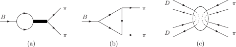
Figure 1: Contributions from inelastic FSI.

The inelastic FSI has been also evaluated as the absorptive part of charmed meson loops shown in Figs. 1(a) and 1(b) CCS . The two unknown cutoff parameters, appearing in the form factors associated with the three-meson vertices, were fixed by the measured $B\to\pi K$ branching ratios. Note that these parameters should be the same for $B\to\pi K$ and $B\to\pi\pi$ in the SU(3) limit. Applying the same formalism to the latter, FSI can not resolve the $B\to\pi\pi$ puzzle, even allowing reasonable SU(3) breaking effects for the cutoff parameters. This result is understandable: the absorptive amplitudes from Figs. 1(a) and 1(b) are more or less orthogonal to the short-distance QCD penguin amplitudes in the $B\to\pi\pi$ decays, so that their effect is minor. Hence, the conclusion in CCS is the same as in DLLN . That is, the charming penguin is not enough to explain the observed $B\to\pi\pi$ branching ratios.

Then additional dispersive amplitudes must be taken into account in CCS . Those from Figs. 1(a) and 1(b), though calculable in the framework of CCS , were not considered. If considered, they, also contributing to the $B\to\pi K$ decays, would change the earlier predictions. Therefore, a brand new mechanism, the dispersive amplitude from the meson annihilation $D\bar{D}\to\pi\pi$ shown in Fig. 1(c), was introduced. There is no corresponding diagram for the $B\to\pi K$ decays. However, this amplitude is beyond the theoretical framework, i.e., it can not be expressed in terms of the Feynman rules derived in CCS . The four free parameters, namely, the two cutoff parameters involved in Figs. 1(a) and 1(b), and the real and imaginary contributions from Fig. 1(c), were then determined by the four pieces of the $B\to\pi\pi$ data: the three branching ratios and the direct CP asymmetry $A_{CP}(B^{0}\to\pi^{\mp}\pi^{\pm})$. That is, the $B^{0}\to\pi^{0}\pi^{0}$ branching ratio has been treated as an input. The point of CCS is to predict the direct CP asymmetries of the $B^{0}\to\pi^{0}\pi^{0}$ and $B^{\pm}\to\pi^{\pm}\pi^{0}$ decays, using the parameters fixed above.

The rescattering among the final states of the $B\to PP$ decays with $P=\pi$, $K$, and $\eta$ has been studied in CHY . These elastic FSI effects were parameterized in terms of two strong phases, which, together with the $B\to\pi$ and $B\to K$ form factors, and the chiral enhancement scale, were then determined by a global fit to the data, including the measured $B^{0}\to\pi^{0}\pi^{0}$ branching ratio. Nevertheless, the feature of the elastic FSI effects, i.e., the correlated decrease and increase of the $B^{0}\to\pi^{\mp}\pi^{\pm}$ and $B^{0}\to\pi^{0}\pi^{0}$ branching ratios, respectively, was noticed CHY . A FSI phase difference between the two $B\to\pi\pi$ isospin amplitudes with $I=0$, $1$ has been introduced in KP0601 , which was then varied to fit the $B\to\pi\pi$ data. Therefore, no explanation for the large $B^{0}\to\pi^{0}\pi^{0}$ branching ratio was provided from the viewpoint of FSI.

There exist other global fits based on different parametrizations for the charmless $B$ meson decays. For example, the large ratio $C/T$ was extracted by fitting the quark-amplitude parametrization to the $B\to\pi\pi$ data BFRPR ; Y03 ; Charng ; HM04 ; CGRS ; Ligeti04 ; WZ ; BHLD . No responsible mechanism was addressed, though the largeness of $C$ was translated into the largeness of the QCD penguin with an internal $t$ quark and/or of the exchange amplitudes in BFRPR . The QCDF formalism, in which the twist-3 spectator and annihilation amplitudes with the end-point singularities were parameterized as mentioned in Sec. III, has been implemented into a global fit to the data Du ; Alek ; CWW . To reach a better fit, the free parameters involved in QCDF must take different values for the $B\to PP$, $PV$, $VP$ modes. These parameters have been tuned to account for the $B\to\pi\pi$ data in KP0601 . As emphasized before, the analysis must be also applied to other modes in order to obtain a consistent picture: the parameters preferred in KP0601 lead to a large real $C/T$, which is not favored by the data of the $B\to\pi K$ direct CP asymmetries as stated in Sec. III.

After carefully investigating the proposals available in the literature, we have found that none of them can really resolve the $B\to\pi\pi$ puzzle. The NLO PQCD analysis has confirmed that it is unlikely to accommodate the $B\to\pi\pi$, $\rho\rho$ data simultaneously (the NLO PQCD predictions are consistent with the $B\to\rho\rho$ data). The $B\to\pi\pi$ decays have been studied in the framework of light-cone sum rules (LCSR) KMMM , where a small $B^{0}\to\pi^{0}\pi^{0}$ branching ratio was also observed. Since there is only little difference between the sum rules for the $B\to\pi\pi$ and $B\to\rho\rho$ modes, we expect that the conclusion from LCSR will be the same as from PQCD. The resolution with the input of the NLO SCET jet function into QCDF BY05 does not survive the constraint from the $B\to\rho\rho$ data, and renders the $B^{0}\to\pi^{\mp}K^{\pm}$ and $B^{\pm}\to\pi^{0}K^{\pm}$ direct CP asymmetries deviate more away from the measured values. We conclude that the $B\to\rho\rho$ data have seriously constrained the possibility of resolving the $B\to\pi\pi$ puzzle in the available theoretical approaches.

We thank H.Y. Cheng, C.K. Chua, D. Pirjol, D. Yang, and R. Zwicky for useful discussions. This work was supported by the National Science Council of R.O.C. under Grant No. NSC-94-2112-M-001-001, by the Taipei branch of the National Center for Theoretical Sciences, and by the U.S. Department of Energy under Grant No. DE-FG02-90ER40542.

Appendix A Transverse Helicity Amplitudes

In this Appendix we present the factorization formulas for the transverse helicity amplitudes:

$$F_{Ne4}(a) = 16\pi C_{F}m_{B}^{2}\int_{0}^{1}dx_{1}dx_{2}\int_{0}^{\infty}b_{1}db_{1}\,b_{2}db_{2}\,\phi_{B}(x_{1},b_{1})$$ (34)

$$\times r_{3}\,\bigg{\{}\left[\phi_{2}^{T}(\overline{x_{2}})+2r_{2}\phi_{2}^{v}(\overline{x_{2}})+r_{2}x_{2}\left(\phi_{2}^{v}(\overline{x_{2}})+\phi_{2}^{a}(\overline{x_{2}})\right)\right]E_{e}(t)h_{e}(A,B,b_{1},b_{2},x_{2})$$

$$\;\;\;\;\;\;\;\;\;\;\;\;+r_{2}\left(\phi_{2}^{v}(\overline{x_{2}})-\phi_{2}^{a}(\overline{x_{2}})\right)E_{e}(t^{\prime})h_{e}(A^{\prime},B^{\prime},b_{2},b_{1},x_{1})\bigg{\}}\;,$$

$$F_{Te4}(a) = 32\pi C_{F}m_{B}^{2}\int_{0}^{1}dx_{1}dx_{2}\int_{0}^{\infty}b_{1}db_{1}\,b_{2}db_{2}\,\phi_{B}(x_{1},b_{1})$$ (35)

$$\times r_{3}\,\bigg{\{}\left[\phi_{2}^{T}(\overline{x_{2}})-2r_{2}\phi_{2}^{a}(\overline{x_{2}})-r_{2}x_{2}\left(\phi_{2}^{v}(\overline{x_{2}})+\phi_{2}^{a}(\overline{x_{2}})\right)\right]E_{e}(t)h_{e}(A,B,b_{1},b_{2},x_{2})$$

$$\;\;\;\;\;\;\;\;\;\;\;\;+r_{2}\left(\phi_{2}^{v}(\overline{x_{2}})-\phi_{2}^{a}(\overline{x_{2}})\right)E_{e}(t^{\prime})h_{e}(A^{\prime},B^{\prime},b_{2},b_{1},x_{1})\bigg{\}}\;,$$

$$F_{Ne6}(a) = F_{Te6}(a)\ =\ 0\;,$$ (36)

$$F_{Na4}(a) = 16\pi C_{F}m_{B}^{2}\,r_{2}r_{3}\int_{0}^{1}dx_{2}dx_{3}\int_{0}^{\infty}b_{2}db_{2}\,b_{3}db_{3}\,$$ (37)

$$\times\bigg{\{}\left[(1-x_{3})\left(\phi_{2}^{v}(\overline{x_{2}})\phi_{3}^{a}(\overline{x_{3}})+\phi_{2}^{a}(\overline{x_{2}})\phi_{3}^{v}(\overline{x_{3}})\right)+(1+x_{3})\left(\phi_{2}^{v}(\overline{x_{2}})\phi_{3}^{v}(\overline{x_{3}})+\phi_{2}^{a}(\overline{x_{2}})\phi_{3}^{a}(\overline{x_{3}})\right)\right]$$

$$\;\;\;\;\;\;\times E_{a}(t)h_{e}(A,B,b_{2},b_{3},x_{3})$$

$$\;\;\;\;\;\;-\left[(2-x_{2})\left(\phi_{2}^{v}(\overline{x_{2}})\phi_{3}^{v}(\overline{x_{3}})+\phi_{2}^{a}(\overline{x_{2}})\phi_{3}^{a}(\overline{x_{3}})\right)-x_{2}\left(\phi_{2}^{v}(\overline{x_{2}})\phi_{3}^{a}(\overline{x_{3}})+\phi_{2}^{a}(\overline{x_{2}})\phi_{3}^{v}(\overline{x_{3}})\right)\right]$$

$$\;\;\;\;\;\;\times E_{a}(t^{\prime})h_{e}(A^{\prime},B^{\prime},b_{3},b_{2},x_{2})\bigg{\}}\;,$$

$$= 16\pi C_{F}m_{B}^{2}\,r_{2}r_{3}\int_{0}^{1}dx_{2}dx_{3}\int_{0}^{\infty}b_{2}db_{2}\,b_{3}db_{3}\,$$

$$\times\bigg{\{}\left[x_{3}\left(\phi_{2}^{v}(\overline{x_{2}})-\phi_{2}^{a}(\overline{x_{2}})\right)\left(\phi_{3}^{v}(\overline{x_{3}})-\phi_{3}^{a}(\overline{x_{3}})\right)+\left(\phi_{2}^{v}(\overline{x_{2}})+\phi_{2}^{a}(\overline{x_{2}})\right)\left(\phi_{3}^{v}(\overline{x_{3}})+\phi_{3}^{a}(\overline{x_{3}})\right)\right]$$

$$\;\;\;\;\;\;\times E_{a}(t)h_{e}(A,B,b_{2},b_{3},x_{3})$$

$$\;\;\;\;\;\;-\left[(1-x_{2})\left(\phi_{2}^{v}(\overline{x_{2}})+\phi_{2}^{a}(\overline{x_{2}})\right)\left(\phi_{3}^{v}(\overline{x_{3}})+\phi_{3}^{a}(\overline{x_{3}})\right)+\left(\phi_{2}^{v}(\overline{x_{2}})-\phi_{2}^{a}(\overline{x_{2}})\right)\left(\phi_{3}^{v}(\overline{x_{3}})-\phi_{3}^{a}(\overline{x_{3}})\right)\right]$$

$$\;\;\;\;\;\;\times E_{a}(t^{\prime})h_{e}(A^{\prime},B^{\prime},b_{3},b_{2},x_{2})\bigg{\}}\;,$$

$$F_{Ta4}(a) = -\,32\pi C_{F}m_{B}^{2}\,r_{2}r_{3}\int_{0}^{1}dx_{2}dx_{3}\int_{0}^{\infty}b_{2}db_{2}\,b_{3}db_{3}\,$$ (38)

$$\times\bigg{\{}\left[(1-x_{3})\left(\phi_{2}^{v}(\overline{x_{2}})\phi_{3}^{v}(\overline{x_{3}})+\phi_{2}^{a}(\overline{x_{2}})\phi_{3}^{a}(\overline{x_{3}})\right)+(1+x_{3})\left(\phi_{2}^{v}(\overline{x_{2}})\phi_{3}^{a}(\overline{x_{3}})+\phi_{2}^{a}(\overline{x_{2}})\phi_{3}^{v}(\overline{x_{3}})\right)\right]$$

$$\;\;\;\;\;\;\times E_{a}(t)h_{e}(A,B,b_{2},b_{3},x_{3})$$

$$\;\;\;\;\;\;-\left[(2-x_{2})\left(\phi_{2}^{v}(\overline{x_{2}})\phi_{3}^{a}(\overline{x_{3}})+\phi_{2}^{a}(\overline{x_{2}})\phi_{3}^{v}(\overline{x_{3}})\right)-x_{2}\left(\phi_{2}^{v}(\overline{x_{2}})\phi_{3}^{v}(\overline{x_{3}})+\phi_{2}^{a}(\overline{x_{2}})\phi_{3}^{a}(\overline{x_{3}})\right)\right]$$

$$\;\;\;\;\;\;\times E_{a}(t^{\prime})h_{e}(A^{\prime},B^{\prime},b_{3},b_{2},x_{2})\bigg{\}}\;,$$

$$= 32\pi C_{F}m_{B}^{2}\,r_{2}r_{3}\int_{0}^{1}dx_{2}dx_{3}\int_{0}^{\infty}b_{2}db_{2}\,b_{3}db_{3}\,$$

$$\times\bigg{\{}\left[x_{3}\left(\phi_{2}^{v}(\overline{x_{2}})-\phi_{2}^{a}(\overline{x_{2}})\right)\left(\phi_{3}^{v}(\overline{x_{3}})-\phi_{3}^{a}(\overline{x_{3}})\right)-\left(\phi_{2}^{v}(\overline{x_{2}})+\phi_{2}^{a}(\overline{x_{2}})\right)\left(\phi_{3}^{v}(\overline{x_{3}})+\phi_{3}^{a}(\overline{x_{3}})\right)\right]$$

$$\;\;\;\;\;\;\times E_{a}(t)h_{e}(A,B,b_{2},b_{3},x_{3})$$

$$\;\;\;\;\;\;+\left[(1-x_{2})\left(\phi_{2}^{v}(\overline{x_{2}})+\phi_{2}^{a}(\overline{x_{2}})\right)\left(\phi_{3}^{v}(\overline{x_{3}})+\phi_{3}^{a}(\overline{x_{3}})\right)-\left(\phi_{2}^{v}(\overline{x_{2}})-\phi_{2}^{a}(\overline{x_{2}})\right)\left(\phi_{3}^{v}(\overline{x_{3}})-\phi_{3}^{a}(\overline{x_{3}})\right)\right]$$

$$\;\;\;\;\;\;\times E_{a}(t^{\prime})h_{e}(A^{\prime},B^{\prime},b_{3},b_{2},x_{2})\bigg{\}}\;,$$

$$F_{Na6}(a) = 32\pi C_{F}m_{B}^{2}\int_{0}^{1}dx_{2}dx_{3}\int_{0}^{\infty}b_{2}db_{2}\,b_{3}db_{3}\,$$ (39)

$$\times\bigg{\{}r_{2}\left(\phi_{2}^{v}(\overline{x_{2}})+\phi_{2}^{a}(\overline{x_{2}})\right)\phi_{3}^{T}(\overline{x_{3}})E_{a}(t)h_{e}(A,B,b_{2},b_{3},x_{3})$$

$$\;\;\;\;\;\;+r_{3}\phi_{2}^{T}(\overline{x_{2}})\left(\phi_{3}^{v}(\overline{x_{3}})-\phi_{3}^{a}(\overline{x_{3}})\right)E_{a}(t^{\prime})h_{e}(A^{\prime},B^{\prime},b_{3},b_{2},x_{2})\bigg{\}}\;,$$

$$F_{Ta6}(a) = 2\,F_{Na6}(a)\;,$$ (40)

$${\cal M}_{Ne4}(a^{\prime}) = 32\pi C_{F}\frac{\sqrt{2N_{c}}}{N_{c}}m_{B}^{2}\,r_{3}\int_{0}^{1}dx_{1}dx_{2}dx_{3}\int_{0}^{\infty}b_{1}db_{1}\,b_{3}db_{3}\,\phi_{B}(x_{1},b_{1})$$ (41)

$$\times\bigg{\{}(1-x_{3})\phi_{2}^{T}(\overline{x_{2}})\left(\phi_{3}^{v}(\overline{x_{3}})-\phi_{3}^{a}(\overline{x_{3}})\right)E^{\prime}_{e}(t)h_{n}(A,B,b_{1},b_{3})$$

$$\;\;\;\;\;\;+\left[x_{3}\phi_{2}^{T}(\overline{x_{2}})\left(\phi_{3}^{v}(\overline{x_{3}})-\phi_{3}^{a}(\overline{x_{3}})\right)-2r_{2}(x_{2}+x_{3})\left(\phi_{2}^{v}(\overline{x_{2}})\phi_{3}^{v}(\overline{x_{3}})+\phi_{2}^{a}(\overline{x_{2}})\phi_{3}^{a}(\overline{x_{3}})\right)\right]$$

$$\;\;\;\;\;\;\times E^{\prime}_{e}(t^{\prime})h_{n}(A^{\prime},B^{\prime},b_{1},b_{3})\bigg{\}}\;,$$

$$= 32\pi C_{F}\frac{\sqrt{2N_{c}}}{N_{c}}m_{B}^{2}\,r_{3}\int_{0}^{1}dx_{1}dx_{2}dx_{3}\int_{0}^{\infty}b_{1}db_{1}\,b_{3}db_{3}\,\phi_{B}(x_{1},b_{1})$$

$$\times\bigg{\{}(1-x_{3})\phi_{2}^{T}(\overline{x_{2}})\left(\phi_{3}^{v}(\overline{x_{3}})-\phi_{3}^{a}(\overline{x_{3}})\right)E^{\prime}_{e}(t)h_{n}(A,B,b_{1},b_{3})$$

$$\;\;\;\;\;\;+\left[x_{3}\phi_{2}^{T}(\overline{x_{2}})\left(\phi_{3}^{v}(\overline{x_{3}})-\phi_{3}^{a}(\overline{x_{3}})\right)-r_{2}(x_{2}+x_{3})\left(\phi_{2}^{v}(\overline{x_{2}})+\phi_{2}^{a}(\overline{x_{2}})\right)\left(\phi_{3}^{v}(\overline{x_{3}})+\phi_{3}^{a}(\overline{x_{3}})\right)\right.$$

$$\left.\;\;\;\;\;\;\;\;\;\;\;-r_{2}(x_{2}+x_{3})\left(\phi_{2}^{v}(\overline{x_{2}})-\phi_{2}^{a}(\overline{x_{2}})\right)\left(\phi_{3}^{v}(\overline{x_{3}})-\phi_{3}^{a}(\overline{x_{3}})\right)\right]E^{\prime}_{e}(t^{\prime})h_{n}(A^{\prime},B^{\prime},b_{1},b_{3})\bigg{\}}\;,$$

$${\cal M}_{Te4}(a^{\prime}) = 64\pi C_{F}\frac{\sqrt{2N_{c}}}{N_{c}}m_{B}^{2}\,r_{3}\int_{0}^{1}dx_{1}dx_{2}dx_{3}\int_{0}^{\infty}b_{1}db_{1}\,b_{3}db_{3}\,\phi_{B}(x_{1},b_{1})$$ (42)

$$\times\bigg{\{}(1-x_{3})\phi_{2}^{T}(\overline{x_{2}})\left(\phi_{3}^{v}(\overline{x_{3}})-\phi_{3}^{a}(\overline{x_{3}})\right)E^{\prime}_{e}(t)h_{n}(A,B,b_{1},b_{3})$$

$$\;\;\;\;\;\;+\left[x_{3}\phi_{2}^{T}(\overline{x_{2}})\left(\phi_{3}^{v}(\overline{x_{3}})-\phi_{3}^{a}(\overline{x_{3}})\right)+2r_{2}(x_{2}+x_{3})\left(\phi_{2}^{v}(\overline{x_{2}})\phi_{3}^{a}(\overline{x_{3}})+\phi_{2}^{a}(\overline{x_{2}})\phi_{3}^{v}(\overline{x_{3}})\right)\right]$$

$$\;\;\;\;\;\;\times E^{\prime}_{e}(t^{\prime})h_{n}(A^{\prime},B^{\prime},b_{1},b_{3})\bigg{\}}\;,$$

$$= 64\pi C_{F}\frac{\sqrt{2N_{c}}}{N_{c}}m_{B}^{2}\,r_{3}\int_{0}^{1}dx_{1}dx_{2}dx_{3}\int_{0}^{\infty}b_{1}db_{1}\,b_{3}db_{3}\,\phi_{B}(x_{1},b_{1})$$

$$\times\bigg{\{}(1-x_{3})\phi_{2}^{T}(\overline{x_{2}})\left(\phi_{3}^{v}(\overline{x_{3}})-\phi_{3}^{a}(\overline{x_{3}})\right)E^{\prime}_{e}(t)h_{n}(A,B,b_{1},b_{3})$$

$$\;\;\;\;\;\;+\left[x_{3}\phi_{2}^{T}(\overline{x_{2}})\left(\phi_{3}^{v}(\overline{x_{3}})-\phi_{3}^{a}(\overline{x_{3}})\right)+r_{2}(x_{2}+x_{3})\left(\phi_{2}^{v}(\overline{x_{2}})+\phi_{2}^{a}(\overline{x_{2}})\right)\left(\phi_{3}^{v}(\overline{x_{3}})+\phi_{3}^{a}(\overline{x_{3}})\right)\right.$$

$$\left.\;\;\;\;\;\;\;\;\;\;\;-r_{2}(x_{2}+x_{3})\left(\phi_{2}^{v}(\overline{x_{2}})-\phi_{2}^{a}(\overline{x_{2}})\right)\left(\phi_{3}^{v}(\overline{x_{3}})-\phi_{3}^{a}(\overline{x_{3}})\right)\right]E^{\prime}_{e}(t^{\prime})h_{n}(A^{\prime},B^{\prime},b_{1},b_{3})\bigg{\}}\;,$$

$${\cal M}_{Ne5}(a^{\prime}) = -{\cal M}_{Ne4}(a^{\prime})\;,$$ (43)

$${\cal M}_{Te5}(a^{\prime}) = -{\cal M}_{Te4}(a^{\prime})\;,$$ (44)

$${\cal M}_{Ne6}(a^{\prime}) = -\,32\pi C_{F}\frac{\sqrt{2N_{c}}}{N_{c}}m_{B}^{2}\,r_{2}\int_{0}^{1}dx_{1}dx_{2}dx_{3}\int_{0}^{\infty}b_{1}db_{1}\,b_{3}db_{3}\,\phi_{B}(x_{1},b_{1})$$ (45)

$$\times x_{2}\left(\phi_{2}^{v}(\overline{x_{2}})+\phi_{2}^{a}(\overline{x_{2}})\right)\phi_{3}^{T}(\overline{x_{3}})\left[E^{\prime}_{e}(t)h_{n}(A,B,b_{1},b_{3})+E^{\prime}_{e}(t^{\prime})h_{n}(A^{\prime},B^{\prime},b_{1},b_{3})\right]\;,$$

$${\cal M}_{Te6}(a^{\prime}) = 2\,{\cal M}_{Ne6}(a^{\prime})\;,$$ (46)

$${\cal M}_{Na4}(a^{\prime}) = -\,64\pi C_{F}\frac{\sqrt{2N_{c}}}{N_{c}}m_{B}^{2}\,r_{2}r_{3}\int_{0}^{1}dx_{1}dx_{2}dx_{3}\int_{0}^{\infty}b_{1}db_{1}\,b_{3}db_{3}\,\phi_{B}(x_{1},b_{1})$$ (47)

$$\times\left(\phi_{2}^{v}(\overline{x_{2}})\phi_{3}^{v}(\overline{x_{3}})+\phi_{2}^{a}(\overline{x_{2}})\phi_{3}^{a}(\overline{x_{3}})\right)E^{\prime}_{a}(t^{\prime})h_{n}(A^{\prime},B^{\prime},b_{3},b_{1})\;,$$

$$= -\,32\pi C_{F}\frac{\sqrt{2N_{c}}}{N_{c}}m_{B}^{2}\,r_{2}r_{3}\int_{0}^{1}dx_{1}dx_{2}dx_{3}\int_{0}^{\infty}b_{1}db_{1}\,b_{3}db_{3}\,\phi_{B}(x_{1},b_{1})$$

$$\times\bigg{\{}\left(\phi_{2}^{v}(\overline{x_{2}})+\phi_{2}^{a}(\overline{x_{2}})\right)\left(\phi_{3}^{v}(\overline{x_{3}})+\phi_{3}^{a}(\overline{x_{3}})\right)+\left(\phi_{2}^{v}(\overline{x_{2}})-\phi_{2}^{a}(\overline{x_{2}})\right)\left(\phi_{3}^{v}(\overline{x_{3}})-\phi_{3}^{a}(\overline{x_{3}})\right)\bigg{\}}$$

$$\;\;\;\;\;\;\times E^{\prime}_{a}(t^{\prime})h_{n}(A^{\prime},B^{\prime},b_{3},b_{1})\;,$$

$${\cal M}_{Ta4}(a^{\prime}) = 128\pi C_{F}\frac{\sqrt{2N_{c}}}{N_{c}}m_{B}^{2}\,r_{2}r_{3}\int_{0}^{1}dx_{1}dx_{2}dx_{3}\int_{0}^{\infty}b_{1}db_{1}\,b_{3}db_{3}\,\phi_{B}(x_{1},b_{1})$$ (48)

$$\times\left(\phi_{2}^{v}(\overline{x_{2}})\phi_{3}^{a}(\overline{x_{3}})+\phi_{2}^{a}(\overline{x_{2}})\phi_{3}^{v}(\overline{x_{3}})\right)E^{\prime}_{a}(t^{\prime})h_{n}(A^{\prime},B^{\prime},b_{3},b_{1})\;,$$

$$= 64\pi C_{F}\frac{\sqrt{2N_{c}}}{N_{c}}m_{B}^{2}\,r_{2}r_{3}\int_{0}^{1}dx_{1}dx_{2}dx_{3}\int_{0}^{\infty}b_{1}db_{1}\,b_{3}db_{3}\,\phi_{B}(x_{1},b_{1})$$

$$\times\bigg{\{}\left(\phi_{2}^{v}(\overline{x_{2}})+\phi_{2}^{a}(\overline{x_{2}})\right)\left(\phi_{3}^{v}(\overline{x_{3}})+\phi_{3}^{a}(\overline{x_{3}})\right)-\left(\phi_{2}^{v}(\overline{x_{2}})-\phi_{2}^{a}(\overline{x_{2}})\right)\left(\phi_{3}^{v}(\overline{x_{3}})-\phi_{3}^{a}(\overline{x_{3}})\right)\bigg{\}}$$

$$\;\;\;\;\;\;\times E^{\prime}_{a}(t^{\prime})h_{n}(A^{\prime},B^{\prime},b_{3},b_{1})\;,$$

$${\cal M}_{Na5}(a^{\prime}) = {\cal M}_{Na4}(a^{\prime})\;,$$ (49)

$${\cal M}_{Ta5}(a^{\prime}) = {\cal M}_{Ta4}(a^{\prime})\;,$$ (50)

$${\cal M}_{Na6}(a^{\prime}) = 32\pi C_{F}\frac{\sqrt{2N_{c}}}{N_{c}}m_{B}^{2}\int_{0}^{1}dx_{1}dx_{2}dx_{3}\int_{0}^{\infty}b_{1}db_{1}\,b_{3}db_{3}\,\phi_{B}(x_{1},b_{1})$$ (51)

$$\times\bigg{\{}\left[r_{3}x_{3}\phi_{2}^{T}(\overline{x_{2}})\left(\phi_{3}^{v}(\overline{x_{3}})-\phi_{3}^{a}(\overline{x_{3}})\right)-r_{2}(1-x_{2})\left(\phi_{2}^{v}(\overline{x_{2}})+\phi_{2}^{a}(\overline{x_{2}})\right)\phi_{3}^{T}(\overline{x_{3}})\right]$$

$$\;\;\;\;\;\;\times E^{\prime}_{a}(t)h_{n}(A,B,b_{3},b_{1})$$

$$\;\;\;\;\;\;+\left[r_{3}(2-x_{3})\phi_{2}^{T}(\overline{x_{2}})\left(\phi_{3}^{v}(\overline{x_{3}})-\phi_{3}^{a}(\overline{x_{3}})\right)-r_{2}(1+x_{2})\left(\phi_{2}^{v}(\overline{x_{2}})+\phi_{2}^{a}(\overline{x_{2}})\right)\phi_{3}^{T}(\overline{x_{3}})\right]$$

$$\;\;\;\;\;\;\times E^{\prime}_{a}(t^{\prime})h_{n}(A^{\prime},B^{\prime},b_{3},b_{1})\bigg{\}}\;,$$

$${\cal M}_{Ta6}(a^{\prime}) = 2\,{\cal M}_{Na6}(a^{\prime})\;.$$ (52)

The quark-loop corrections ${\cal M}^{(q)}_{N,T}$ for $q=u$, $c$, and $t$, and the magnetic-penguin corrections ${\cal M}^{(g)}_{N,T}$ to the transverse components are written as

$${\cal M}^{(q)}_{N} = -16m_{B}^{2}\frac{C_{F}^{2}}{\sqrt{2N_{c}}}\,r_{3}\int_{0}^{1}dx_{1}dx_{2}dx_{3}\int_{0}^{\infty}b_{1}db_{1}b_{2}db_{2}\phi_{B}(x_{1},b_{1})$$ (53)

$$\times\big{\{}\left[\phi_{2}^{T}(\overline{x_{2}})\left(\phi_{3}^{v}(\overline{x_{3}})+\phi_{3}^{a}(\overline{x_{3}})\right)\right.$$

$$\;\;\;\;\;\;\;\;\;\;\;\left.+r_{2}(2+x_{2})\phi_{2}^{v}(\overline{x_{2}})\phi_{3}^{v}(\overline{x_{3}})+r_{2}x_{2}\phi_{2}^{a}(\overline{x_{2}})\phi_{3}^{v}(\overline{x_{3}})+4r_{2}\phi_{2}^{a}(\overline{x_{2}})\phi_{3}^{a}(\overline{x_{3}})\right]$$

$$\;\;\;\;\;\;\times E^{(q)}(t_{q},l^{2})h_{e}(A,B,b_{1},b_{2},x_{2})$$

$$\;\;\;\;\;\;+\,r_{2}\phi_{2}^{v}(\overline{x_{2}})\phi_{3}^{v}(\overline{x_{3}})E^{(q)}(t_{q}^{\prime},l^{\prime 2})h_{e}(A^{\prime},B^{\prime},b_{2},b_{1},x_{1})\big{\}}\;,$$

$${\cal M}^{(q)}_{T} = 0\;,$$ (54)

$${\cal M}^{(g)}_{N} = 16m_{B}^{4}\frac{C_{F}^{2}}{\sqrt{2N_{c}}}\int_{0}^{1}dx_{1}dx_{2}dx_{3}\int_{0}^{\infty}b_{1}db_{1}\,b_{2}db_{2}\,b_{3}db_{3}\,\phi_{B}(x_{1},b_{1})$$ (55)

$$\times\,\Big{\{}\left[-r_{2}(1-x_{2}^{2})\left(\phi_{3}^{v}(\overline{x_{3}})+\phi_{3}^{a}(\overline{x_{3}})\right)\phi_{3}^{T}(\overline{x_{3}})-r_{3}(1+x_{2})x_{3}\phi_{2}^{T}(\overline{x_{2}})\left(\phi_{3}^{v}(\overline{x_{3}})-\phi_{3}^{a}(\overline{x_{3}})\right)\right.$$

$$\left.\;\;\;\;\;\;\;\;\;\;\;-r_{2}r_{3}(1-x_{2})\left(\phi_{2}^{v}(\overline{x_{2}})+\phi_{2}^{a}(\overline{x_{2}})\right)\left(\phi_{3}^{v}(\overline{x_{3}})+\phi_{3}^{a}(\overline{x_{3}})\right)\right.$$

$$\left.\;\;\;\;\;\;\;\;\;\;\;-r_{2}r_{3}x_{3}(1-2x_{2})\left(\phi_{2}^{v}(\overline{x_{2}})-\phi_{2}^{a}(\overline{x_{2}})\right)\left(\phi_{3}^{v}(\overline{x_{3}})-\phi_{3}^{a}(\overline{x_{3}})\right)\right]E_{g}(t_{q})h_{g}(A,B,C,b_{1},b_{2},b_{3},x_{2})$$

$$\;\;\;\;\;\;-r_{2}r_{3}x_{3}\left(\phi_{2}^{v}(\overline{x_{2}})-\phi_{2}^{a}(\overline{x_{2}})\right)\left(\phi_{3}^{v}(\overline{x_{3}})-\phi_{3}^{a}(\overline{x_{3}})\right)E_{g}(t_{q}^{\prime})h_{g}(A^{\prime},B^{\prime},C^{\prime},b_{2},b_{1},b_{3},x_{1})\Big{\}}\;,$$

$${\cal M}^{(g)}_{T} = 32m_{B}^{4}\frac{C_{F}^{2}}{\sqrt{2N_{c}}}\int_{0}^{1}dx_{1}dx_{2}dx_{3}\int_{0}^{\infty}b_{1}db_{1}\,b_{2}db_{2}\,b_{3}db_{3}\,\phi_{B}(x_{1},b_{1})$$ (56)

$$\times\,\Big{\{}\left[-r_{2}(1-x_{2}^{2})\left(\phi_{3}^{v}(\overline{x_{3}})+\phi_{3}^{a}(\overline{x_{3}})\right)\phi_{3}^{T}(\overline{x_{3}})-r_{3}(1+x_{2})x_{3}\phi_{2}^{T}(\overline{x_{2}})\left(\phi_{3}^{v}(\overline{x_{3}})-\phi_{3}^{a}(\overline{x_{3}})\right)\right.$$

$$\left.\;\;\;\;\;\;\;\;\;\;\;+r_{2}r_{3}(1-x_{2})\left(\phi_{2}^{v}(\overline{x_{2}})+\phi_{2}^{a}(\overline{x_{2}})\right)\left(\phi_{3}^{v}(\overline{x_{3}})+\phi_{3}^{a}(\overline{x_{3}})\right)\right.$$

$$\left.\;\;\;\;\;\;\;\;\;\;\;-r_{2}r_{3}x_{3}(1-2x_{2})\left(\phi_{2}^{v}(\overline{x_{2}})-\phi_{2}^{a}(\overline{x_{2}})\right)\left(\phi_{3}^{v}(\overline{x_{3}})-\phi_{3}^{a}(\overline{x_{3}})\right)\right]E_{g}(t_{q})h_{g}(A,B,C,b_{1},b_{2},b_{3},x_{2})$$

$$\;\;\;\;\;\;-r_{2}\left[(1-x_{2})\phi_{2}^{v}(\overline{x_{2}})\phi_{3}^{T}(\overline{x_{3}})-r_{3}(1-2x_{2})\phi_{2}^{v}(\overline{x_{2}})\phi_{3}^{v}(\overline{x_{3}})-r_{3}\phi_{2}^{v}(\overline{x_{2}})\phi_{3}^{a}(\overline{x_{3}})\right.$$

$$\left.\;\;\;\;\;\;\;\;\;\;\;-r_{3}\phi_{2}^{a}(\overline{x_{2}})\phi_{3}^{v}(\overline{x_{3}})+r_{3}\phi_{2}^{a}(\overline{x_{2}})\phi_{3}^{a}(\overline{x_{3}})\right]E_{g}(t_{q}^{\prime})h_{g}(A^{\prime},B^{\prime},C^{\prime},b_{2},b_{1},b_{3},x_{1})\Big{\}}\;.$$

The definitions of all the variables and the convolution factors in the above expressions are referred to LMS05 .

References

• (1) Heavy Flavor Averaging Group, hep-ex/0505100; updated in http://www.slac.stanford.edu/xorg/hfag.
• (2) Y.Y. Keum, H-n. Li, and A.I. Sanda, Phys Lett. B 504, 6 (2001); Phys. Rev. D 63, 054008 (2001).
• (3) C.D. LΓΌ, K. Ukai, and M.Z. Yang, Phys. Rev. D 63, 074009 (2001).
• (4) H-n. Li, S. Mishima, and A.I. Sanda, Phys. Rev. D 72, 114005 (2005).
• (5) F.J. Botella, D. London, and J.P. Silva, Phys. Rev. D 73, 071501 (2006).
• (6) Y.D. Yang, R.M. Wang, and G.R. Lu, Phys. Rev. D 73, 015003 (2006).
• (7) S. Baek, F.J. Botella, D. London, and J.P. Silva, Phys. Rev. D 72, 114007 (2005).
• (8) J.F. Cheng, Y.N. Gao, C.S. Huang, and X.H. Wu, hep-ph/0512268.
• (9) M. Beneke, G. Buchalla, M. Neubert, and C.T. Sachrajda, Phys. Rev. Lett. 83, 1914 (1999); Nucl. Phys. B591, 313 (2000); Nucl. Phys. B606, 245 (2001).
• (10) M. Beneke and D. Yang, Nucl. Phys. B736, 34 (2006).
• (11) C.W. Bauer, D. Pirjol, I.Z. Rothstein, and I.W. Stewart, Phys. Rev. D 70, 054015 (2004).
• (12) C.W. Bauer, I.Z. Rothstein, and I.W. Stewart, hep-ph/0510241.
• (13) C.K. Chua, W.S. Hou, and K.C. Yang, Phys. Rev. D 65, 096007 (2002); Mod. Phys. Lett. A18, 1763 (2003).
• (14) H.Y. Cheng, C.K. Chua, and A. Soni, Phys. Rev. D 71, 014030 (2005).
• (15) A. Deandrea, M. Ladisa, V. Laporta, G. Nardulli, and P. Santorelli, hep-ph/0508083.
• (16) Y.Y. Charng and H-n. Li, Phys. Rev. D 71, 014036 (2005).
• (17) Y. Grossman, A. Hocker, Z. Ligeti, and D. Pirjol, Phys. Rev. D 72, 094033 (2005).
• (18) Y. Li and C.D. LΓΌ, Phys. Rev. D 73, 014024 (2006).
• (19) C.H. Chen, hep-ph/0601019.
• (20) T. Kurimoto, H-n. Li, and A.I. Sanda, Phys. Rev. D 65, 014007 (2002).
• (21) P. Ball, V.M. Braun, Y. Koike, and K. Tanaka, Nucl. Phys. B529, 323 (1998).
• (22) M. Beneke and M. Neubert, Nucl. Phys. B675, 333 (2003).
• (23) P.K. Das and K.C. Yang, Phys. Rev. D 71, 094002 (2005); Y.D. Yang, R.M. Wang, and G.R. Lu, Phys. Rev. D 72, 015009 (2005); W.J. Zou and Z.J. Xiao, Phys. Rev. D 72, 094026 (2005).
• (24) S. Mishima and A.I. Sanda, Prog. Theor. Phys. 110, 549 (2003); Phys.Rev. D 69, 054005 (2004).
• (25) P. Ball and V.M. Braun, Phys. Rev. D 58, 094016 (1998).
• (26) P. Ball and R. Zwicky, Phys. Rev. D 71, 014029 (2005).
• (27) A.L. Kagan, Phys. Lett. B 601, 151 (2004); hep-ph/0407076.
• (28) C.H. Chen, Y.Y. Keum, and H-n. Li, Phys. Rev. D 66, 054013 (2002).
• (29) H-n. Li and S. Mishima, Phys. Rev. D 71, 054025 (2005).
• (30) P. Colangelo, G. Nardulli, N. Paver, and Riazuddin, Z. Phys. C 45, 575 (1990); M. Ciuchini, E. Franco, G. Martinelli, and L. Silvestrini, Nucl. Phys. B501, 271 (1997).
• (31) A.R. Williamson and J. Zupan, hep-ph/0601214.
• (32) H.Y. Cheng and K.C. Yang, Phys. Lett. B 511, 40 (2001).
• (33) M. Beneke and S. Jager, hep-ph/0512101.
• (34) M. Beneke and S. Jager, hep-ph/0512351.
• (35) M. Ladisa, V. Laporta, G. Nardulli, and P. Santorelli, Phys. Rev. D 70, 114025 (2004).
• (36) E. Kou and T.N. Pham, hep-ph/0601272.
• (37) Y.Y. Charng and H-n. Li, Phys. Lett. B. 594, 185 (2004).
• (38) T. Yoshikawa, Phys. Rev. D 68, 054023 (2003); S. Mishima and T. Yoshikawa, Phys. Rev. D 70, 094024 (2004).
• (39) A.J. Buras, R. Fleischer, S. Recksiegel, and F. Schwab, Phys. Rev. Lett. 92, 101804 (2004); Nucl.Phys. B697, 133 (2004).
• (40) X.G. He and B. McKellar, hep-ph/0410098.
• (41) C.W. Chiang, M. Gronau, J.L. Rosner, and D.A. Suprun Phys. Rev. D 70, 034020 (2004).
• (42) Z. Ligeti, Int. J. Mod. Phys. A 20, 5105 (2005).
• (43) Y.L. Wu and Y.F. Zhou, Phys. Rev. D 71, 021701 (2005).
• (44) S. Baek, P. Hamel, D. London, A. Datta, and D.A. Suprun, Phys. Rev. D 71, 057502 (2005).
• (45) D.s. Du, J.f. Sun, D.s. Yang, and G.h. Zhu, Phys. Rev. D 67, 014023 (2003).
• (46) R. Aleksan, P. F.Β Giraud, V. Morenas, O. Pene, and A. S. Safir, Phys. Rev. D 67, 094019 (2003).
• (47) W.N. Cottingham, I.B. Whittingham, and F.F. Wilson, Phys. Rev. D 71, 077301 (2005).
• (48) A. Khodjamirian, Th. Mannel, M. Melcher, and B. Melic, Phys. Rev. D 72, 094012 (2005).