Abstract

The gauge-invariant three-gluon vertex obtained from the pinch technique is characterized by thirteen nonzero form factors, which are given in complete generality for unbroken gauge theory at one loop. The results are given in $d$ dimensions using both dimensional regularization and dimensional reduction, including the effects of massless gluons and arbitrary representations of massive gauge bosons, fermions, and scalars. We find interesting relations between the functional forms of the contributions from gauge bosons, fermions, and scalars. These relations hold only for the gauge-invariant pinch technique vertex and are d-dimensional incarnations of supersymmetric nonrenormalization theorems which include finite terms. The form factors are shown to simplify for $N=1,2$, and $4$ supersymmetry in various dimensions. In four-dimensional non-supersymmetric theories, eight of the form factors have the same functional form for massless gluons, quarks, and scalars, when written in a physically motivated tensor basis. For QCD, these include the tree-level tensor structure which has prefactor $\beta_{0}=(11N_{c}-2N_{f})/3$, another tensor with prefactor $4N_{c}-N_{f}$, and six tensors with $N_{c}-N_{f}$. In perturbative calculations our results lead naturally to an effective coupling for the three-gluon vertex, $\widetilde{\alpha}(k_{1}^{2},k_{2}^{2},k_{3}^{2})$, which depends on three momenta and gives rise to an effective scale $Q_{eff}^{2}(k_{1}^{2},k_{2}^{2},k_{3}^{2})$ which governs the behavior of the vertex. The effects of nonzero internal masses $M$ are important and have a complicated threshold and pseudo-threshold structure. A three-scale effective number of flavors $N_{F}(k_{1}^{2}/M^{2},k_{2}^{2}/M^{2},k_{3}^{2}/M^{2})$ is defined. The results of this paper are an important part of a gauge-invariant dressed skeleton expansion and a related multi-scale analytic renormalization scheme. In this approach the scale ambiguity problem is resolved since physical kinematic invariants determine the arguments of the couplings.

1 Introduction: Gauge-Invariant Green’s Functions

The main purpose of this paper is to analyze the structure of the gauge-invariant three-gluon vertex [1], calculate the fourteen form factors at one loop, and outline some of the phenomenological applications. Before proceeding, it is worthwhile to review the motivation and current status of gauge-invariant Green’s functions.

In the conventional formulation of gauge field theories, the manifest gauge-invariance of the original action is lost upon quantization, simply because one has to fix a gauge in order to perform calculations. Generically, Greens’s functions are gauge-dependent and thus not physical by themselves. Only the particular combinations of Green’s functions which form physical observables must be gauge-invariant. In many theoretical studies, however, one would like to consider individual Green’s functions and extract physical meaning from them [2]. For example, studies of the infrared behavior of gauge theory using Dyson-Schwinger equations [3] often rely on gauge-dependent truncation schemes which one hopes are not too brutal. The existence of gauge-invariant two-point functions is crucial for defining meaningful resummed propagators [4], particularly near threshold, for the construction of effective charges [5], for a postulated dressed-skeleton expansion of QCD [6], and for justifying renormalon analyses [7].

Thus there is strong motivation for gauge-invariant Green’s functions with physical content. We will now briefly discuss the relationship between three different approaches to gauge-invariant Green’s functions : (1) the Pinch Technique (PT), (2) the Background Field Method (BFM), and (3) the $\star$ effective Lagrangian scheme of Kennedy and Lynn. All three approaches will lead to the same Green’s functions.

The pinch technique (PT) was first constructed by Cornwall [2] in order to study gauge-invariant Dyson-Schwinger equations and dynamical gluon mass generation, but the approach is much more generally applicable. In the PT approach, unique gauge-invariant Green’s functions are constructed by explicitly rearranging Feynman diagrams using elementary Ward identities (WI) as the guiding principle. Longitudinal momenta from triple-gauge-boson vertices and gauge propagators inside of loops hit other vertices and thus generate inverse propagators (via WI’s), which, in turn, cancel (or pinch) some internal propagators. In this way, certain parts of Green’s functions are reduced to parts of lower $n$-point functions, and should properly be included in the latter.

As an example of the PT, consider the gluon (or massive gauge boson) self-energy. The conventional self-energy is gauge-dependent and physically meaningless by itself. However, when embedded in any physical process, there will be associated parts of vertex and box graphs which undergo the reduction described above and thus have the same tensor and kinematic structure as the gluon propagator. These pinched parts are then added to the conventional gauge-dependent self-energy, yielding a gauge-invariant self-energy and gluon propagator that has the correct asymptotic UV behavior dictated by the renormalization group equation. The resulting two-point function has numerous positive attributes [4][8][5][9][10], including uniqueness, resummability, analyticity, unitarity, and a natural relation to optical theorem, from which it can also be derived [4][11].

Resumming these two-point functions leads to physical effective charges, $\acute{a}la$ Grunberg[12], which can be extended to the supersymmetric case and leads to an analytic improvement of gauge coupling unification with smooth threshold behavior [13].

This method has been applied to a variety of Green’s functions [1][14][15] [16][17], with applications to electroweak phenomenology [18][19]. In particular, the gauge-invariant three-gluon vertex was first constructed in [1] to one-loop order, where the authors showed that the vertex satisfies a relatively simple abelian-like Ward identity. However, the integrals were not evaluated, so that little could be said about the individual form factors except that the UV divergent term in the tree level tensor structure is correct. The main motivation of this paper is to extend this work by evaluating the integrals for the fourteen form factors, and expressing the results in a convenient tensor basis for phenomenological applications. In doing so, an interesting structure emerges, in which the contributions of gluons(G), quarks(Q), and scalars(S) are intimately related. These relations are closely linked to supersymmetry and conformal symmetry, and in particular the $N=4$ non-renormalization theorems. For all form factors $F$ in dimensions $d$, we find that

$$F_{G}+4F_{Q}+(10-d)F_{S}=0,$$ (1)

which encodes the vanishing contribution of the $N=4$ supermultiplet in four dimensions. Similar relations have been found in the context of supersymmetric scattering amplitudes [20][21]. In Appendix E, the effects of internal masses are discussed, and the above sum rule becomes modified

$$F_{MG}+4F_{MQ}+(9-d)F_{MS}=0,$$ (2)

for internal massive gauge bosons (MG), fermions (MQ), and scalar (MS). The external gluons remain massless and unbroken, so the internal gauge bosons might be the heavy $X_{\mu},Y_{\mu}$ bosons of $SU(5)$, for example. In [22], supersymmetric relations were found for electroweak gauge boson four-point scattering amplitudes.

The PT method has been explicitly extended beyond one-loop [23][24][25], has recently been proven to exist to all orders in perturbation theory [26][27][28][29], and interestingly, each Green’s function is equal to the corresponding Green’s function of the Background Field Method (BFM) in quantum Feynman gauge $\xi_{Q}=1$, a result suggested in [30][31]. Heuristically, this is due to the fact that there are no longitudinal (pinching) momenta in the gauge propagator or the elementary vertices in this special gauge.

The Background Field Method (BFM) [32] constructs manifestly gauge invariant Green’s functions in the following way. First, the field variable($A$) in the path integral is separated into a background($B$) and quantum($Q$) field, $A=B+Q$. Only the quantum field $Q$ propagates in loops, since it is a variable of functional integration. In contrast, the background field $B$ appears only in external legs. By judiciously choosing the gauge-fixing function, one arrives at an effective action which remains manifestly invariant under background field gauge-transformations $\delta B^{a}_{\mu}=-f^{abc}\omega^{b}B^{c}_{\mu}+{1\over g}\partial_{\mu}\omega^{a}$. Furthermore, derivatives of the BFM effective action with respect to the background field $B$ yield the same 1PI Green’s functions as the conventional effective action with a nonstandard gauge-fixing. Thus, it can be shown [32] that the correct S-matrix is obtained by sewing together trees composed of 1PI Green’s functions of $B$ fields. In doing so, one can fix the gauge of $B$, which propagates only at tree level, independently of the gauge fixing of $Q$. For example, convenient non-covariant gauges might be used for the trees while BFM Feynman gauge $\xi_{Q}=1$ (BFMFG) can be used for the loops.

The correspondence between the PT and BFM is not surprising, since the BFM is a formulation of gauge theory where Green’s functions of the gauge field are manifestly (background) gauge-invariant. Although this is true for all values of the quantum gauge-fixing parameter $\xi_{Q}$, it is only for the special value $\xi_{Q}=1$ that the BFM Green’s functions also have the correct kinematic structure of the irreducible PT Green’s functions. Alternatively, it has been shown [31] that applying the PT algorithm to the BFM for $\xi_{Q}\neq 1$ leads back to the canonical ($\xi_{Q}=1$) PT Green’s functions.

Finally, in the $\star$ scheme of Kennedy and Lynn [33], a gauge-invariant effective Lagrangian was constructed for electroweak four-fermion processes by explicitly rearranging the one loop corrections. As in the pinch technique, vertex parts must be added to would-be two point functions to yield genuine two-point functions. One particular motivation is that fact that the photon acquires a spurious mass from its mixing with $Z^{0}$, $\Pi_{\gamma Z}(q^{2}=0)\neq 0$, unless the correct vertex parts are added. The resulting effective charges, $\alpha_{\star}(q^{2})$ and $s^{2}_{\star}(q^{2})$ are in fact precisely equal to the corresponding pinch-technique effective charges at one loop, including all finite terms and threshold dependence [8].

Thus, all three methods for constructing physical gauge-invariant Green’s functions lead to the same results, which in the this paper will be referred to as either PT or PT/BFMFG Green’s functions.

The organization of this paper is as follows. In section 2, we will discuss the general structure of the gauge-invariant three-gluon vertex, which is constrained by the Ward identity and Bose symmetry. Two convenient tensor bases and their relation are discussed. In section 3, the main results of this paper are given. First, the nontrivial supersymmetric relations between the gluon, quark, and scalar contributions to each form factor are discussed. The explicit results for the form factors are given in two different bases for massless internal particles, with the full mass effects relegated to Appendix E. In section 4, we briefly discuss the phenomenological application to physical scattering processes, where we derive an effective coupling for the three-gluon vertex, $\widetilde{\alpha}(k_{1}^{2},k_{2}^{2},k_{3}^{2})$, and an effective scale, $Q^{2}_{eff}(k_{1}^{2},k_{2}^{2},k_{3}^{2})$, both of which depend on three distinct gluon virtualities. In section 5, the phenomenological effects of internal masses are discussed. A complicated threshold and pseudo-threshold structure emerges. Furthermore, a three-scale effective number of flavors $N_{F}(k_{1}^{2}/M^{2},k_{2}^{2}/M^{2},k_{3}^{2}/M^{2})$ is defined. Conclusions are given in section 6. In appendix A, a brief outline of the calculational method is given, and some basic one- and two-point integrals are given. Appendix B is devoted to a thorough discussion of the massive triangle integral, and analytic continuations are given for each kinematic region. Appendix C collects some useful results for special functions. Appendix D explains the corrections to the form factors when a supersymmetric regularization is used. Finally Appendix E gives explicitly the corrections to the form factors arising from internal massive gauge bosons, fermions, and scalars.

2 General Structure of the Three-Gluon Vertex

2.1 Symmetries

One of the most important aspects of the gauge-invariant three-gluon vertex discussed in this paper is the relatively simple Ward identity it satisfies, which has the same form as the Ward ID satisfied by the tree level vertex. This was proven at one-loop in the original paper by Cornwall and Papavassiliou [1] using the explicit one-loop result, which is the gluon part of Eqs.(68,3) below. It is straightforward to show that the fermion and scalar parts also satisfy the same Ward identity (just as in QED). Furthermore, the equivalence of the BFMFG and PT to all orders [26] allows one to write the Ward identity satisfied by the three-gluon vertex to all orders as

$$p_{3}^{\mu_{3}}\Gamma_{\mu_{1}\mu_{2}\mu_{3}}^{abc}(p_{1},p_{2},p_{3})=f^{adc}\Big{(}t_{\mu_{1}\mu_{2}}(p_{2})\delta^{db}+\Pi_{\mu_{1}\mu_{2}}^{db}(p_{2})\Big{)}-f^{adc}\Big{(}t_{\mu_{1}\mu_{2}}(p_{1})\delta^{da}+\Pi_{\mu_{1}\mu_{2}}^{da}(p_{1})\Big{)},$$ (3)

plus two other equations which are cyclic permutations. The transverse tensor $t_{\mu\nu}(p)=p^{2}g_{\mu\nu}-p_{\mu}p_{\nu}$ comes from the tree level term. Here all momenta are defined to be incoming and all labels are defined in counter-clockwise fashion, as shown in Fig. 1. This Ward identity represents a great simplification compared to the usual Slavnov-Taylor identities satisfied by the conventional gauge-dependent three-gluon vertex, which involves the gluon propagator, the ghost propagator, and the ghost-ghost-gluon vertex function. The self-energy function in the above equation is not the usual gauge-dependent self-energy, but rather the gauge-invariant pinch technique self energy, which is the only self energy discussed in this paper.

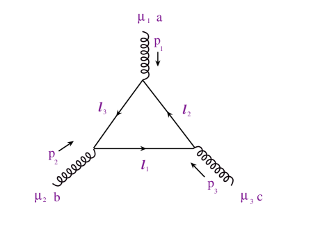
Figure 1: The notation and loop momentum routing used throughout this paper. The internal particle could be a gauge boson, ghost, quark, or scalar.

An immediate consequence is that the longitudinal ($L$) part of the vertex, defined as the part which contributes to the above Ward ID, must have only the antisymmetric color factor $f^{abc}$ so long as gluons conserve the color charge, $\Pi_{\mu\nu}^{ab}(q)=\delta^{ab}\Pi_{\mu\nu}(q)$. As far as we know, the transverse ($T$) part of the vertex (defined by $p_{3}^{\mu_{3}}\Gamma_{\mu_{1}\mu_{2}\mu_{3}}^{abc(T)}(p_{1},p_{2},p_{3})=0$) is not required to be proportional to $f^{abc}$, but may in principle contain $d^{abc}$ terms. Nevertheless, no such terms appear at one or two loop order, and so in the subsequent discussion we take

$$\Gamma_{\mu_{1}\mu_{2}\mu_{3}}^{abc}(p_{1},p_{2},p_{3})=f^{abc}\Gamma_{\mu_{1}\mu_{2}\mu_{3}}(p_{1},p_{2},p_{3}),$$ (4)

in terms of which the Ward identity becomes

$$p_{3}^{\mu_{3}}\Gamma_{\mu_{1}\mu_{2}\mu_{3}}(p_{1},p_{2},p_{3})=t_{\mu_{1}\mu_{2}}(p_{2})(1+\Pi(p_{2}^{2}))-t_{\mu_{1}\mu_{2}}(p_{1})(1+\Pi(p_{1}^{2})).$$ (5)

Bose symmetry, the fact that 3 identical particles are entering the vertex, and the properties of $f^{abc}$ imply definite properties of $\Gamma_{\mu_{1}\mu_{2}\mu_{3}}(p_{1},p_{2},p_{3})$ under the interchange of labels. In particular, defining the five elements of the permutation group ${\cal S}_{3}$ to act by

$$g_{123} = \left(\begin{array}[]{ccc}(\mu_{1},p_{1})\rightarrow(\mu_{2},p_{2})\\ (\mu_{2},p_{2})\rightarrow(\mu_{3},p_{3})\\ (\mu_{3},p_{3})\rightarrow(\mu_{1},p_{1})\end{array}\right)\;\;\;\;\;\;\;\;g_{12}=\left(\begin{array}[]{ccc}(\mu_{1},p_{1})\rightarrow(\mu_{2},p_{2})\\ (\mu_{2},p_{2})\rightarrow(\mu_{1},p_{1})\end{array}\right)$$ (11)

$$g_{23} = \left(\begin{array}[]{ccc}(\mu_{2},p_{2})\rightarrow(\mu_{3},p_{3})\\ (\mu_{3},p_{3})\rightarrow(\mu_{2},p_{2})\end{array}\right)\;\;\;\;\;\;\;\;g_{31}=\left(\begin{array}[]{ccc}(\mu_{3},p_{3})\rightarrow(\mu_{1},p_{1})\\ (\mu_{1},p_{1})\rightarrow(\mu_{3},p_{3})\end{array}\right)$$ (16)

and $g_{321}=g_{123}^{-1}$ one finds that $(g_{123},g_{321},g_{12},g_{23},g_{31})$ yields $(+,+,-,-,-)$ when acting on $\Gamma_{\mu_{1}\mu_{2}\mu_{3}}(p_{1},p_{2},p_{3})$.

The nonabelian nature of the permutation group ${\cal S}_{3}$ prevents one from finding a basis in which all of the tensors are eigenstates of all of these operators. Thus, aesthetic and physical principles must guide us in choosing convenient bases, two of which are discussed momentarily.

2.2 Two Convenient Bases

Let us consider the most general tensor structure. The three index Lorentz covariant tensor must be constructed out of the metric $g_{\mu\nu}$ and the momenta ($p_{i}^{\mu}$). Since the momenta are not independent, $p_{1}+p_{2}+p_{3}=0$, simple combinatorics implies that there are in general 14 independent tensor components, 6 of which have one power of momenta and also the metric, and 8 of which have 3 powers of momenta. Many different basis choices can be made, although we will use essentially two.

In the subsequent discussion, some efficient notation will prove useful. This is summarized in Table 1.

$${\rm Table\;\;I.\;Definition\;\;of\;\;tensor\;\;abbreviations}$$

    $$001\equiv g_{\mu_{1}\mu_{2}}p_{1\mu_{3}} 002\equiv g_{\mu_{1}\mu_{2}}p_{2\mu_{3}} 200\equiv g_{\mu_{2}\mu_{3}}p_{2\mu_{1}} 300\equiv g_{\mu_{2}\mu_{3}}p_{3\mu_{1}} 030\equiv g_{\mu_{3}\mu_{1}}p_{3\mu_{2}} 010\equiv g_{\mu_{3}\mu_{1}}p_{1\mu_{2}} 211\equiv p_{2\mu_{1}}p_{1\mu_{2}}p_{1\mu_{3}} 212\equiv p_{2\mu_{1}}p_{1\mu_{2}}p_{2\mu_{3}} 232\equiv p_{2\mu_{1}}p_{3\mu_{2}}p_{2\mu_{3}} 332\equiv p_{3\mu_{1}}p_{3\mu_{2}}p_{2\mu_{3}} 331\equiv p_{3\mu_{1}}p_{3\mu_{2}}p_{1\mu_{3}} 311\equiv p_{3\mu_{1}}p_{1\mu_{2}}p_{1\mu_{3}} 312\equiv p_{3\mu_{1}}p_{1\mu_{2}}p_{2\mu_{3}} 231\equiv p_{2\mu_{1}}p_{3\mu_{2}}p_{1\mu_{3}}$$                            

Thus, each tensor is rewritten as a 3 slot object, where slots correspond to $\mu_{1},\mu_{2},\mu_{3}$ in that order, and the content of each slot is either ‘1’,‘2’, or ‘3’ to represent momentum $p_{1},p_{2},p_{3}$, or a ‘0’, which must occur in pairs and represents that those two indices are connected by the metric tensor.

The most naive thing to do would be to just eliminate one momenta, say $p_{3}=-p_{1}-p_{2}$ and use the following 14 basis tensors : $100$, $200$, $010$, $020$, $001$, $002$, $111$, $112$, $121$, $211$, $122$, $212$, $221$, $222$. This is not very useful since the explicit Bose symmetry between the three gluons has been broken, and thus delicate relations between the form factors will have to enforce it.

The $\pm$ Basis

A more natural choice is obtained by starting from a manifestly symmetric, but redundant basis, which has 36 possible basis tensors, 9 with one power of momenta, and 27 with three powers of momenta. As a step towards our final basis, we find it convenient to eliminate all such tensors with momenta $p_{1}^{\mu_{1}},p_{2}^{\mu_{2}}$, or $p_{3}^{\mu_{3}}$, i.e. anything with 1 in the first slot, 2 in second slot or 3 in the third slot. This yields the 14 basis tensors $001$, $002$, $200$, $300$, $030$, $010$, $211$, $212$, $232$, $332$, $331$, $311$, $231$, $312$, which are shown in Table 1. Note that under the action of $g_{123}$ we have $200\rightarrow 030,300\rightarrow 010,211\rightarrow 232,311\rightarrow 212$, etc. Also, notice that $200$ and $300$ are interchanged by the action of $g_{23}$, while $211$ and $212$ are interchanged by the action of $g_{12}$, etc. Thus, it is convenient to take appropriate linear combinations such that one of these interchange operators is diagonal for each tensor. Such basis tensors are

$$\hat{a}_{12} = (00-)=001-002,\;\;\;\hat{a}_{23}=(-00)=200-300,\;\;\;\hat{a}_{31}=(0\!-\!0)=030-010$$

$$\hat{b}_{12} = (00+)=001+002,\;\;\;\hat{b}_{23}=(+00)=200+300,\;\;\;\hat{b}_{31}=(0\!+\!0)=030+010$$

$$\hat{c}_{12} = (\!+\!+\!-\!),\;\;\;\hat{c}_{23}=(\!-\!+\!+\!),\;\;\;\hat{c}_{31}=(\!+\!-\!+\!)$$

$$\hat{d}_{12} = (\!-\!-\!+\!),\;\;\;\hat{d}_{23}=(\!+\!-\!-\!),\;\;\;\hat{d}_{31}=(\!-\!+\!-\!)$$ (17)

$$\hat{h} = (\!-\!-\!-\!),\;\;\;\hat{s}=(\!+\!+\!+\!),$$

where the notation means $(\!\pm\!\pm\!\pm\!)\;\equiv\;(2\pm 3,3\pm 1,1\pm 2)$, so that $(\!+\!+\!-\!)=231-232+211-212+331-332+311-312$, etc. The subscripts are chosen because, for example, $\hat{a}_{12}$ is an eigenstate of $g_{12}$, etc.

Suppressing indices and momentum dependence, the three-gluon vertex is then written as

$$\Gamma=(A_{12}\hat{a}_{12}+B_{12}\hat{b}_{12}+C_{12}\hat{c}_{12}+D_{12}\hat{d}_{12}+{\rm perms})+S\hat{s}+H\hat{h},$$ (18)

where the lower case letters represent the basis tensors, while the upper case letters are the form factors, which depend on $p_{1}^{2},p_{2}^{2},$ and $p_{3}^{2}$. In addition to indicating which basis tensors they are associated with, the subscripts on form factors also indicate the ordering of momenta in the arguments. For example, $A_{12}=A(p_{1}^{2},p_{2}^{2}|p_{3}^{2})$, $A_{23}=A(p_{2}^{2},p_{3}^{2}|p_{1}^{2})$, $A_{31}=A(p_{3}^{2},p_{1}^{2}|p_{2}^{2})$, and the first two arguments are either symmetric or antisymmetric. The behavior of these form factors under ${\cal S}_{3}$ can be inferred from the behavior of the basis tensors under ${\cal S}_{3}$ (which will be discussed momentarily), along with the overall requirement for the vertex given below Eq. 11. One finds that $A(x,y|z)=+A(y,x|z)$, and thus $A_{12}=A_{21}$, etc. Similarly, $B_{12}=-B_{21}$, $C_{12}=C_{21}$, and $D_{12}=-D_{21}$. $H$ is totally invariant under the interchange or permutation of any momenta, while $S$ goes to $-S$ under any interchange of momenta, but is invariant under a cyclic permutation $g_{123}$.

It is straightforward to see that under the action of the permutation operator ($g_{123}$) these fourteen basis tensors are organized into four triplets, $\{\hat{a}_{12},\hat{a}_{23},\hat{a}_{31}\}$, $\{\hat{b}_{12},\hat{b}_{23},\hat{b}_{31}\}$, $\{\hat{c}_{12},\hat{c}_{23},\hat{c}_{31}\}$, $\{\hat{d}_{12},\hat{d}_{23},\hat{d}_{31}\}$, as well as $\hat{h}$ and $\hat{s}$. The latter two are eigenstates of all five operators.

Consider the properties of $\{\hat{a}_{12},\hat{a}_{23},\hat{a}_{31}\}$ under the permutation group. It is easy to see that under the action of any element $g_{i}$, we have

$$\left(\begin{array}[]{cccc}\hat{a}_{12}\\ \hat{a}_{23}\\ \hat{a}_{31}\end{array}\right)\rightarrow g_{i}\left(\begin{array}[]{cccc}\hat{a}_{12}\\ \hat{a}_{23}\\ \hat{a}_{31}\end{array}\right),$$ (19)

with the matrices given by

$$g_{123} =\left(\begin{array}[]{cccc}0&1&0\\ 0&0&1\\ 1&0&0\end{array}\right)\;\;\;\;\;g_{321}=\left(\begin{array}[]{cccc}0&0&1\\ 1&0&0\\ 0&1&0\end{array}\right)$$ (26)

$$g_{12} =-\left(\begin{array}[]{cccc}1&0&0\\ 0&0&1\\ 0&1&0\end{array}\right)\;\;\;\;g_{23}=-\left(\begin{array}[]{ccc}0&0&1\\ 0&1&0\\ 1&0&0\end{array}\right)\;\;\;\;g_{31}=-\left(\begin{array}[]{ccc}0&1&0\\ 1&0&0\\ 0&0&1\end{array}\right)$$ (36)

The transformation rules are identical for $\{c_{ij}\}$, and similar for $\{b_{ij}\}$ and $\{d_{ij}\}$ with the only change being that there is no minus sign in the three interchange operators $g_{12},g_{23}$ and $g_{31}$.

The basis constructed above (Eq.(2.2)) will be called the $\pm$ basis. As discussed later, this basis is the most convenient for phenomenology and furthermore the form factors exhibit particularly simple relations between the gluon, quark, and scalar contributions (Eqs.(3.4,3.4)).

However, the $\pm$ basis as it stands does not contain the tree level tensor structure. Thus, one is naturally led to diagonalizing the permutation operator $g_{123}$. Clearly, this is the most symmetric choice and, more importantly, one of the resulting eigenvectors is the tree level tensor structure.

In the triplet representation of ${\cal S}_{3}$, $g_{123}$ is diagonalized by the similarity transformation

$$S={1\over\sqrt{3}}\left(\begin{array}[]{ccc}1&1&1\\ 1&\lambda&\overline{\lambda}\\ 1&\overline{\lambda}&\lambda\end{array}\right)\;\;\;\;\;\;\;\;S^{-1}g_{123}S\;\equiv\;\widetilde{g}_{123}=\left(\begin{array}[]{ccc}1&0&0\\ 0&\lambda&0\\ 0&0&\overline{\lambda}\end{array}\right),$$ (37)

where $\lambda=\exp{({2i\pi\over 3})}=-{\litfont{1\over 2}}+i{\sqrt{3}\over 2}$, $\overline{\lambda}=\lambda^{*}$ are cube roots of unity. This results in new basis tensors and form factors

$$\left(\begin{array}[]{ccc}\hat{a}_{0}\\ \hat{a}_{+}\\ \hat{a}_{-}\end{array}\right) \equiv \sqrt{3}S^{-1}\left(\begin{array}[]{ccc}\hat{a}_{12}\\ \hat{a}_{23}\\ \hat{a}_{31}\end{array}\right)=\left(\begin{array}[]{ccc}1&1&1\\ 1&\overline{\lambda}&\lambda\\ 1&\lambda&\overline{\lambda}\end{array}\right)\left(\begin{array}[]{ccc}\hat{a}_{12}\\ \hat{a}_{23}\\ \hat{a}_{31}\end{array}\right)$$ (50)

$$\left(\begin{array}[]{ccc}A_{0}\\ A_{+}\\ A_{-}\end{array}\right) \equiv {1\over\sqrt{3}}S\left(\begin{array}[]{ccc}A_{12}\\ A_{23}\\ A_{31}\end{array}\right)={1\over 3}\left(\begin{array}[]{ccc}1&1&1\\ 1&\lambda&\overline{\lambda}\\ 1&\overline{\lambda}&\lambda\end{array}\right)\left(\begin{array}[]{ccc}A_{12}\\ A_{23}\\ A_{31}\end{array}\right).$$ (63)

This procedure is repeated identically for the $(b,B)$, $(c,C)$, and $(d,D)$ basis tensors and form factors.

Notice that $\hat{a}_{0}=g_{\mu_{1}\mu_{2}}(p_{1}-p_{2})_{\mu_{3}}+g_{\mu_{2}\mu_{3}}(p_{2}-p_{3})_{\mu_{1}}+g_{\mu_{3}\mu_{1}}(p_{3}-p_{1})_{\mu_{2}}$ is the tree level tensor, which is why the extra factors of $\sqrt{3}$ were included above.

The transformation properties for the basis tensors $\hat{a}_{i}$ and $\hat{c}_{i}$ are deduced from $\widetilde{g}_{123}$ given above, $\widetilde{g}_{321}={\rm diag}(1,\overline{\lambda},\lambda)$, and

$$\widetilde{g}_{12}=-\left(\begin{array}[]{cccc}1&0&0\\ 0&0&1\\ 0&1&0\end{array}\right)\;\;\;\;\widetilde{g}_{23}=-\left(\begin{array}[]{ccc}1&0&0\\ 0&0&\lambda\\ 0&\overline{\lambda}&0\end{array}\right)\;\;\;\;\widetilde{g}_{31}=-\left(\begin{array}[]{ccc}1&0&0\\ 0&0&\overline{\lambda}\\ 0&\lambda&0\end{array}\right),$$ (64)

while the transformation properties of the form factors are deduced by demanding that behavior given below Eq.(11) is respected. For example, since $\hat{a}_{-}\rightarrow-\overline{\lambda}\hat{a}_{+}$ under $\widetilde{g}_{23}$, we find $A_{-}\rightarrow\lambda A_{+}$ so that $A_{-}\hat{a}_{-}\rightarrow-A_{-}\hat{a}_{-}$. For $(b,B)$ and $(d,D)$, the only change in the above is that there is not a minus sign in $\widetilde{g}_{12},\widetilde{g}_{23},$ and $\widetilde{g}_{31}$.

We have not touched $\hat{h}$ and $\hat{s}$, as these are already eigenstates of all five operators $(g_{123},g_{321},g_{12},g_{23},g_{31})$, with eigenvalues $(++---)$ and $(+++++)$, respectively.

We will call the above constructed basis the symmetric $\pm$ basis. Note that any basis can be symmetrized in the same manner by diagonalizing the permutation operator $g_{123}$. The basis we started with in Eq.(2.2) is motivated by (a) its simple and symmetric construction from only metrics and $(p_{i+1}{\pm}p_{i-1})_{\mu_{i}}$, (b) it is the most convenient basis for perturbative calculations, as will be discussed in section 4, and (c) The individual form factors have a relatively simple form, as will be discussed in section 3.

The LT Basis

For some theoretical studies, another convenient basis is determined by the distinction between transverse ($T$) and longitudinal ($L$) tensors [34][35]. The $L$ tensors contribute to the Ward ID (or the more complicated Slavnov-Taylor ID for the gauge dependent vertex) while the $T$ tensors satisfy homogeneous equations $p_{3}^{\mu_{3}}\Gamma^{(T)}_{\mu_{1}\mu_{2}\mu_{3}}=0$. This is a very convenient basis for evaluating the loop corrections to the vertex, since the $L$ and $T$ parts separate, as described in Appendix A.

The $\pm$ basis and the $LT$ basis are complementary in the following sense. The $\pm$ basis is constructed out of combinations of longitudinal ($+$) and transverse ($-$) momenta, so that for example $(00+)=g_{\mu_{1}\mu_{2}}(p_{1\mu_{3}}+p_{2\mu_{3}})=-g_{\mu_{1}\mu_{2}}p_{3\mu_{3}}$ vanishes if the $\mu_{3}$ index is contracted into a conserved current. Meanwhile, the $LT$ basis distinguishes between parts of the vertex that do ($T$) and do not ($L$) vanish when dotted with longitudinal momenta. These straightforward relations to current conservation and Ward identities are essentially the reason these two bases are the most convenient to work with.

In our notation, the vertex can be written in the $LT$ basis as $\Gamma=\Gamma_{L}+\Gamma_{T}$, where

$$\Gamma_{L} = (\overline{A}_{12}\overline{a}_{12}+\overline{B}_{12}\overline{b}_{12}+\overline{C}_{12}\overline{c}_{12}+{\rm perms})+\overline{S}\overline{s}$$

$$\Gamma_{T} = (\overline{F}_{12}\overline{f}_{12}+{\rm perms})+\overline{H}\overline{h},$$ (65)

and the bar distinguishes this $LT$ basis from the $\pm$ basis defined above in Eq.(2.2). The relation between basis tensors is given by

$$\overline{a}_{12} = 001-002=\hat{a}_{12}$$ (66)

$$\overline{b}_{12} = 001+002=\hat{b}_{12}$$

$$\overline{c}_{12} = 211-212-(p_{1}\!\cdot\!p_{2})(001-002)={1\over 4}(\hat{c}_{12}-\hat{d}_{23}+\hat{d}_{31}-\hat{h})-(p_{1}\!\cdot\!p_{2})\hat{a}_{12}$$

$$\overline{f}_{12} = (p_{1}\!\cdot\!p_{2})\Big{(}(p_{2}\!\cdot\!p_{3})001-(p_{3}\!\cdot\!p_{1})002\Big{)}-\Big{(}(p_{2}\!\cdot\!p_{3})211-(p_{3}\!\cdot\!p_{1})212\Big{)}$$

$$= {(p_{1}\!\cdot\!p_{2})\over 2}\Big{(}-p_{3}^{2}\hat{a}_{12}+(p_{1}^{2}-p_{2}^{2})\hat{b}_{12}\Big{)}$$

$$+ {1\over 8}\Big{(}p_{3}^{2}(\hat{c}_{12}-\hat{d}_{23}+\hat{d}_{31}-\hat{h})+(p_{1}^{2}-p_{2}^{2})(\hat{d}_{12}-\hat{c}_{23}+\hat{c}_{31}-\hat{s})\Big{)}$$

$$\overline{h} = 231-312-\Big{(}(p_{1}\!\cdot\!p_{2})(030-300)+(p_{2}\!\cdot\!p_{3})(001-010)+(p_{3}\!\cdot\!p_{1})(200-002)\Big{)}$$

$$= {1\over 4}(\hat{h}+\hat{c}_{12}+\hat{c}_{23}+\hat{c}_{31})+{\litfont{1\over 2}}\Big{(}p_{3}^{2}\hat{a}_{12}-(p_{1}^{2}-p_{2}^{2})\hat{b}_{12}+p_{1}^{2}\hat{a}_{23}-(p_{2}^{2}-p_{3}^{2})\hat{b}_{23}$$

$$+ p_{2}^{2}\hat{a}_{31}-(p_{3}^{2}-p_{1}^{2})\hat{b}_{31}\Big{)}$$

$$\overline{s} = 231+312={1\over 4}(\hat{s}+\hat{d}_{12}+\hat{d}_{23}+\hat{d}_{31}),$$

and we used $(p_{1}\!\cdot\!p_{2})=(p_{3}^{2}-p_{1}^{2}-p_{2}^{2})/2$. This implies the relation between form factors

$$A_{12} = \overline{A}_{12}-(p_{1}\!\cdot\!p_{2})\overline{C}_{12}-{p_{3}^{2}\over 2}\Big{(}(p_{1}\!\cdot\!p_{2})\overline{F}_{12}-\overline{H}\Big{)}$$

$$B_{12} = \overline{B}_{12}+{p_{1}^{2}-p_{2}^{2}\over 2}\Big{(}(p_{1}\!\cdot\!p_{2})\overline{F}_{12}-\overline{H}\Big{)}$$ (67)

$$C_{12} = {1\over 4}\Big{(}\overline{H}+\overline{C}_{12}+{p_{3}^{2}\over 2}\overline{F}_{12}+{p_{1}^{2}-p_{3}^{2}\over 2}\overline{F}_{31}+{p_{2}^{2}-p_{3}^{2}\over 2}\overline{F}_{23}\Big{)}$$

$$D_{12} = {1\over 4}\Big{(}\overline{S}+\overline{C}_{23}-\overline{C}_{31}+{p_{1}^{2}\over 2}\overline{F}_{23}-{p_{2}^{2}\over 2}\overline{F}_{31}+{p_{1}^{2}-p_{2}^{2}\over 2}\overline{F}_{12}\Big{)}$$

$$H = {1\over 4}\Big{(}\overline{H}-\overline{C}_{12}-{p_{3}^{2}\over 2}\overline{F}_{12}-\overline{C}_{23}-{p_{1}^{2}\over 2}\overline{F}_{23}-\overline{C}_{31}-{p_{2}^{2}\over 2}\overline{F}_{31}\Big{)}$$

$$S = {1\over 4}\Big{(}\overline{S}+{p_{2}^{2}-p_{1}^{2}\over 2}\overline{F}_{12}+{p_{3}^{2}-p_{2}^{2}\over 2}\overline{F}_{23}+{p_{1}^{2}-p_{3}^{2}\over 2}\overline{F}_{31}\Big{)},$$

The unwritten form factors ($A_{23}$, etc.) and basis tensors can be obtained trivially from the above equations by cyclic permutation ($g_{123}$). In doing so it is useful to keep in mind the properties described under Eq.(18), along with $\overline{F}_{ij}=\overline{F}_{ji}$, $\overline{A}_{ij}=\overline{A}_{ji}$, $\overline{B}_{ij}=-\overline{B}_{ji}$, $\overline{C}_{ij}=\overline{C}_{ji}$, while $\overline{H}$ and $\overline{S}$ have the same transformation properties as $H$ and $S$, respectively.

3 Results for the Form Factors

In this section, we will present the results for the form factors in arbitrary dimension $d$ using dimensional regularization (DREG), for gluons in the adjoint representation, and massless quarks and scalars in arbitrary representations. The corrections due to supersymmetric regularization and massive fermions, scalars, and gauge bosons are given in detail in Appendices D and E, respectively.

The gauge invariant vertex at one loop can be written as

$$g \!\!\!\!\!\Gamma_{\mu_{1}\mu_{2}\mu_{3}}^{abc}(p_{1},p_{2},p_{3})=gf^{abc}\Bigg{[}\Gamma_{\mu_{1}\mu_{2}\mu_{3}}^{(0)}(p_{1},p_{2},p_{3})$$ (68)

$$- {ig^{2}\over 2}\Bigg{(}C_{A}G_{\mu_{1}\mu_{2}\mu_{3}}+2\sum_{f}T_{f}N_{f}Q_{\mu_{1}\mu_{2}\mu_{3}}+2\sum_{s}T_{s}N_{s}S_{\mu_{1}\mu_{2}\mu_{3}}\Bigg{)}\Bigg{]}$$

where the gluon ($G$), quark ($Q$), and scalar ($S$) integrals are

$$G_{\mu_{1}\mu_{2}\mu_{3}} = \int{d^{d}l\over(2\pi)^{d}}{1\over l_{1}^{2}l_{2}^{2}l_{3}^{2}}\Bigg{(}\Gamma_{\beta\mu_{1}\gamma}^{F}(l_{2},p_{1},-l_{3})\Gamma_{\gamma\mu_{2}\alpha}^{F}(l_{3},p_{2},-l_{1})\Gamma_{\alpha\mu_{3}\beta}^{F}(l_{1},p_{3},-l_{2})$$

$$+ 2(l_{2}+l_{3})_{\mu_{1}}(l_{3}+l_{1})_{\mu_{2}}(l_{1}+l_{2})_{\mu_{3}}-8l_{1}^{2}(g_{\mu_{1}\mu_{2}}p_{1\mu_{3}}-g_{\mu_{1}\mu_{3}}p_{1\mu_{2}})$$

$$- 8l_{2}^{2}(g_{\mu_{2}\mu_{3}}p_{2\mu_{1}}-g_{\mu_{2}\mu_{1}}p_{2\mu_{3}})-8l_{3}^{2}(g_{\mu_{3}\mu_{1}}p_{3\mu_{2}}-g_{\mu_{3}\mu_{2}}p_{3\mu_{1}})\Bigg{)}$$

$$Q_{\mu_{1}\mu_{2}\mu_{3}} = \int{d^{d}l\over(2\pi)^{d}}{1\over l_{1}^{2}l_{2}^{2}l_{3}^{2}}{\rm Tr}[\gamma_{\mu_{1}}\;\raise 0.6458pt\hbox{/}\kern-4.70001ptl_{3}\gamma_{\mu_{2}}\;\raise 0.6458pt\hbox{/}\kern-4.70001ptl_{1}\gamma_{\mu_{3}}\;\raise 0.6458pt\hbox{/}\kern-4.70001ptl_{2}]$$

$$S_{\mu_{1}\mu_{2}\mu_{3}} = -\int{d^{d}l\over(2\pi)^{d}}{1\over l_{1}^{2}l_{2}^{2}l_{3}^{2}}(l_{2}+l_{3})_{\mu_{1}}(l_{3}+l_{1})_{\mu_{2}}(l_{1}+l_{2})_{\mu_{3}}.$$ (69)

The gluon contribution was first derived in [1] using the pinch technique(PT), and is equivalent to the vertex obtained in the Background Field Method in quantum Feynman gauge(BFMFG). The quark and scalar integrals come straightforwardly from the one loop triangle diagrams. The notation and routing of the integral are defined in Fig.(1) such that $l_{1}=p_{2}+l_{3}$, $l_{2}=p_{3}+l_{1}$, $l_{3}=p_{1}+l_{2}$ and the tree level vertex $\Gamma^{(0)}$ and $\Gamma^{F}$ are defined as

$$\Gamma_{\mu_{1}\mu_{2}\mu_{3}}^{(0)}(p_{1},p_{2},p_{3}) = g_{\mu_{1}\mu_{2}}(p_{1}-p_{2})_{\mu_{3}}+g_{\mu_{2}\mu_{3}}(p_{2}-p_{3})_{\mu_{1}}+g_{\mu_{3}\mu_{1}}(p_{3}-p_{1})_{\mu_{2}}$$

$$\Gamma_{\beta\mu_{1}\gamma}^{F}(l_{2},p_{1},-l_{3}) = 2p_{1\beta}g_{\mu_{1}\gamma}-2p_{1\gamma}g_{\mu_{1}\beta}-(l_{2}+l_{3})_{\mu_{1}}g_{\beta\gamma}.$$ (70)

All massless integrals can be reduced to two basic scalar integrals:

$$J\; {\equiv} \;J(p_{1}^{2},p_{2}^{2},p_{3}^{2})=\int{d^{d}l\over(2\pi)^{d}}{1\over l_{1}^{2}l_{2}^{2}l_{3}^{2}}$$

$$J_{1}\; {\equiv} \;J_{1}(p_{1}^{2})=\int{d^{d}l\over(2\pi)^{d}}{1\over l_{2}^{2}l_{3}^{2}}=\int{d^{d}l\over(2\pi)^{d}}{1\over l^{2}(l+p_{1})^{2}},$$ (71)

These functions, and the massive integrals which are considered later, are summarized in Appendices A and B, where $J$ is written in terms of Clausen functions. In the following we will suppress the momentum arguments and write our results in terms of $J,J_{1},J_{2},J_{3}$.

3.1 (Supersymmetric) relations between gluons, quarks, and scalars

Before presenting the results for individual form factors, which are somewhat lengthy, we will discuss the relationship between the gluon(G), quark(Q), and scalar(S) contributions. We will end up finding relations similar to those found in the context of supersymmetric scattering amplitudes [20][21][36]. For a generic form factor $F$, let us write the one-loop contribution as

$$F=ig^{2}\Big{(}C_{A}F_{G}+2\sum_{f}T_{f}N_{f}F_{Q}+2\sum_{s}T_{s}N_{s}F_{S}\Big{)},$$ (72)

where the coupling constant $ig^{2}$ and group theory factors have been pulled out. The standard notation is used, so that $C_{A}\equiv C_{2}(G)=N_{c}$ for $SU(N_{c})$, and ${\rm Tr}[t^{a}_{f}t^{b}_{f}]=T_{f}\delta^{ab}$. Thus, $F_{Q}$ stands for the contribution of one Dirac fermion in the fundamental representation of $SU(N_{c})$, or, due to a symmetry factor of ${\litfont{1\over 2}}$ for Weyl fermions, the contribution of adjoint gluinos divided by $N_{c}$. Similarly, $F_{S}$ stands for the contribution of one complex scalar in the fundamental representation, or the contribution of a real scalar in the adjoint, divided by $N_{c}$. These identifications will be used shortly.

After explicitly calculating the integrals in Eq.(3), we noticed that the gluon, quark, and scalar contributions have a similar structure for each form factor. To make this explicit, define the following sums for form factor $F$ :

$$\Sigma_{QG}(F) \equiv {(d-2)\over 2}F_{Q}+F_{G}$$

$$\Sigma_{SG}(F) \equiv (d-2)F_{S}-F_{G}.$$ (73)

Although the results for each form factor are often long, these sums are particularly simple, as can be seen in Eqs.(3.3,3.4,3.4). For all form factors in any basis, it also turns out that

$$(d-10)\Sigma_{SG}=8\Sigma_{QG}$$ (74)

and $\Sigma_{QG}$ is always proportional to $d-10$. The above two equations and the results of Eqs.(3.3,3.4,3.4) can be used to determine the $Q$ and $S$ contributions to any form factor, given the gluon contributions written explicitly below. Furthermore, Eqs.(3.1,74) can be combined leading to

$$F_{G}+4F_{Q}+(10-d)F_{S}=0.$$ (75)

Considering the very different origins of each form factor (Eqs.(68,3)), it is remarkable that they are related in such a simple manner. Note that no such analogous relation holds for the gauge dependent vertex [35].

This type of relation hints at supersymmetry. To further understand the content of these relations, we will consider various supersymmetries in $d=4$.

• N=1 From the above definitions, it is clear that a vector superplet $V_{1}$ (gluons plus gluinos) contributes $ig^{2}N_{c}(F_{G}+F_{Q})\equiv ig^{2}N_{c}F_{V_{1}}$ to a generic form factor $F$, while $N_{\Phi}$ chiral superplets contributes $ig^{2}N_{\Phi}({\litfont{1\over 2}}F_{Q}+F_{S})\equiv ig^{2}N_{\Phi}F_{\Phi}$. By the sum rule Eq.(75) in $d=4$, we have $F_{V_{1}}+6F_{\Phi}=0$. Thus any form factor can be written

  $$F=ig^{2}(N_{c}F_{V_{1}}+N_{\Phi}F_{\Phi})={ig^{2}\over 3}\beta_{0}^{(N=1)}F_{V_{1}},$$ (76)

  where $\beta_{0}^{(N=1)}=3N_{c}-{\litfont{1\over 2}}N_{\Phi}$ is the first $\beta$ function coefficient. Hence the contributions of vector and chiral superplets have precisely the same functional form for each form factor. Furthermore, every form factor is proportional to $\beta_{0}$ even though all but one of them are UV finite.

• N=2 Here the vector superplet gives $ig^{2}N_{c}(F_{G}+2F_{Q}+2F_{S})\equiv ig^{2}N_{c}F_{V_{2}}$, while $N_{h}$ hyperplets (a Weyl fermion of each helicity plus a doublet of complex scalars) yield $ig^{2}N_{h}(F_{Q}+2F_{S})\equiv ig^{2}N_{h}F_{h}$. The sum rule Eq.(75) can be written as $F_{V_{2}}+2F_{h}=0$, and thus

  $$F=ig^{2}(N_{c}F_{V_{2}}+N_{h}F_{h})={ig^{2}\over 2}\beta_{0}^{(N=2)}F_{V_{2}},$$ (77)

  where $\beta_{0}^{(N=2)}=2N_{c}-N_{h}$.

• N=4 Here the vector superplet (the only multiplet allowed) contributes $2ig^{2}N_{c}(F_{G}+4F_{Q}+6F_{S})\equiv N_{c}F_{V_{4}}$, which is identically zero by the sum rule, which of course is a consequence of $\beta_{0}^{(N=4)}=0$.

Thus, the similarities between form factors in $d=4$ are related to supersymmetric non-renormalization theorems. In particular, the exact conformal invariance of $N=4$ implies that the gauge-invariant three-gluon Green’s function is not renormalized at any order in perturbation theory. Furthermore, at one-loop order there are not even finite corrections, as reflected in Eq.(75).

Analogous results hold for supersymmetry in $d\neq 4$. Here we must be careful, because in the sum rules and form factors presented in this paper we worked in $d$ dimensions everywhere except in the traces over gamma matrices, where we used the conventional rule of dimensional regularization ${\rm tr}[\gamma_{\mu}\gamma_{\nu}]=4g_{\mu\nu}$, and similarly for other traces. Properly working in integer valued $d$ dimensions, we should use ${\rm tr}[\gamma_{\mu}\gamma_{\nu}]=d_{s}(d)g_{\mu\nu}$, where the spinor dimension of the gamma matrices is

$$d_{s}(d)=\left(\begin{array}[]{ccc}2^{d/2}\\ 2^{(d-1)/2}\end{array}\right)\;\;{\rm for}\;\;\left(\begin{array}[]{ccc}d\;\;{\rm even}\\ d\;\;{\rm odd}\end{array}\right).$$ (78)

Thus $F_{Q_{d}}\equiv{d_{s}(d)\over 4}F_{Q}$ is the contribution of a Dirac fermion in $d$ dimensions, and we have

$$F_{G}+{16\over d_{s}(d)}F_{Q_{d}}+(10-d)F_{S}=0$$ (79)

Rather than using Eq.(79), one can alternatively use Eq.(75) and be sure to count fermion degrees of freedom in terms of $d=4$ spinors. Thus the Weyl fermions of $d=6$ and the Weyl-Majorana fermions of $d=10$ are composed of $2$ and $4$ Weyl fermions of four dimensions, respectively. From this, it is straightforward to show that $d=6,N=2$ and $d=10,N=1$ gauge theory give vanishing contribution to every form factor. For the $d=6,N=1$ case, one finds

$$F={ig^{2}\over 2}\beta_{0}F_{V_{1}}\;\;\;\;\;\;\beta_{0}=2N_{c}-N_{\Phi},$$ (80)

where $\beta_{0}$ is determined from Eq.(88) in $d=6$.

Note that it is not straightforward to analytically continue $d_{s}(d)$ into arbitrary non-integer $d$, which is the reason for the simple dimensional regularization rule. However, the sum rule expressed in Eq.(75) is an analytic function of $d$ and thus represents an analytic continuation of supersymmetric non-renormalization theorems to arbitrary $d$. This is intimately related to the existence of a supersymmetry preserving regulator, dimensional reduction (DRED), where vector degrees of freedom are kept in four dimensions while the integrals are still performed in $d$ dimensions. Around four dimensions, $d=4-2\epsilon$, we have $F_{G}+4F_{Q}+(6+2\epsilon)F_{S}=0$ in dimensional regularization, and we see that the $\epsilon$ term plays the role of the so-called $\epsilon$-ghosts of DRED. We have calculated the form factors in DRED (see Appendix D) and verified that

$$F_{G}+4F_{Q}+6F_{S}=0\;\;\;\;\;\;{(\rm DRED)}.$$ (81)

In the preceding discussion of supersymmetries in various dimensions we implicitly used DRED.

The extension of these relations to the massive case is outlined in Appendix E, where the full effects of internal massive fermions (MQ), massive scalars (MS), and massive gauge bosons (MG) are included, and the sum rule becomes

$$F_{MG}+4F_{MQ}+(9-d)F_{MS}=0$$ (82)

in DREG while in DRED the only change is $9-d$ is replaced by $5$. Note that the external gluons remain massless and unbroken, so the internal massive gauge bosons might be the colored heavy gauge bosons arising in GUT models. The change of $10-d$ in the massless case to $9-d$ in the massive case reflects the fact that massive gauge bosons “eat” one scalar degree of freedom.

It should be emphasized that relations such as Eq.(75) do not exist for the gauge-dependent three-gluon vertex [35], since the gluon contributions depend on the gauge-parameter, while the quarks and scalars do not. Indeed, it is uniquely the pinch technique (or equivalently BFM in quantum Feynman gauge) Green’s function which satisfies this homogeneous sum rule. For example, calculating in the BFM with $\xi_{Q}\neq 1$, leads to a nonzero RHS of Eq.(75).

Since the sum rule applies to all form factors, one finds

$$G_{\mu_{1}\mu_{2}\mu_{3}}+4Q_{\mu_{1}\mu_{2}\mu_{3}}+(10-d)S_{\mu_{1}\mu_{2}\mu_{3}}=0,$$ (83)

which is remarkable given the expressions in Eq.(3). One can explicitly show this by performing the trace in Eq.(3) and some tedious algebra to rearrange the $\Gamma^{F}\Gamma^{F}\Gamma^{F}$ term. This can also be seen in the second order formalism of the BFM [20][21][36].

A similar relation holds for the one-loop gauge-invariant (pinch-technique) gluon two-point function in $d$ dimensions,

$$\Pi_{\mu_{1}\mu_{2}}^{ab}(p)=\delta^{ab}(p^{2}g_{\mu_{1}\mu_{2}}-p_{\mu_{1}}p_{\mu_{2}})\Pi(p^{2})\;{\equiv}\;ig^{2}\delta^{ab}\Big{(}N_{c}G_{\mu_{1}\mu_{2}}+2\sum_{f}T_{f}N_{f}Q_{\mu_{1}\mu_{2}}+2\sum_{s}T_{s}N_{s}S_{\mu_{1}\mu_{2}}\Big{)},$$ (84)

where from Eqs.(87,88) below we find

$$G_{\mu_{1}\mu_{2}}+4Q_{\mu_{1}\mu_{2}}+(10-d)S_{\mu_{1}\mu_{2}}=0.$$ (85)

Unfortunately, analogous relations do not hold for higher gauge-invariant gluon $n$-point functions. This is essentially because the color and spacetime indices mix nontrivially. However, inhomogeneous relations of the form

$$G+4Q+(10-d)S={\rm simple}$$ (86)

still hold [20][21][36], where “simple” means an integral with fewer powers of loop momenta in the numerator. In the four-gluon case, this is just a simple scalar integral with no powers of loop momentum in the numerator. These loop momentum counting rules have been derived in the second order formalism, which is reviewed in [36]. Note that the Ward ID for the four-gluon vertex [17] relates it to the three-gluon vertex, and thus the longitudinal parts of the four-gluon vertex must satisfy the homogeneous sum rules $F_{G}+4F_{Q}+(10-d)F_{S}=0$.

It is interesting to see if extensions of these sum rules apply to two-loop calculations, where the supersymmetric Yukawa vertices must be taken into account. As a first application, the two-loop pinch technique gluon self-energy has been calculated including finite terms. Interestingly, the finite terms do not vanish for $N=4$ SUSY, so it appears that the homogeneous sum rule in Eq.(75) does not have a counterpart at two loops. In any case, the finite parts of the two loop result allow for an improved extraction of the PT couplings from data as well as giving the three loop beta function. This calculation will be reported elsewhere [37].

Now explicit expressions for the form factors will be given, first in the $LT$ basis, and then in the $\pm$ basis.

3.2 The longitudinal form factors

It is straightforward to solve the Ward identity (Eq.(5)) for the ten longitudinal form factors, defined in Eq.(2.2), in terms of the gluon self-energy function $\Pi$ defined by $\Pi_{\mu\nu}^{ab}(p)=\delta^{ab}(p^{2}g_{\mu\nu}-p_{\mu}p_{\nu})\Pi(p^{2})$. Note that this is not the usual gauge-dependent self-energy, but rather the gauge-invariant pinch technique self-energy. At one loop in $d$ dimensions this is given by

$$\Pi(p^{2})=ig^{2}\beta_{0}(d)\int{d^{d}l\over(2\pi)^{d}}{1\over l^{2}(l+p)^{2}},$$ (87)

where $\beta_{0}(d)$ is given by

$$\beta_{0}(d) = {7d-6\over 2(d-1)}C_{2}(G)-{2(d-2)\over(d-1)}\sum_{f}T_{f}N_{f}-{1\over(d-1)}\sum_{s}T_{s}N_{s}$$ (88)

for massless gluons, quarks, and complex scalars. The mass-dependent results are given in section 5 and Appendix E. This result holds for dimensional regularization (DREG), whereas for dimensional reduction (DRED) the gluon coefficient changes from $(7d-6)$ to $(8d-10)$.

The longitudinal form factors are given by

$$\overline{A}_{12} = {\Pi(p_{1}^{2})+\Pi(p_{2}^{2})\over 2}$$

$$\overline{B}_{12} = {\Pi(p_{1}^{2})-\Pi(p_{2}^{2})\over 2}$$ (89)

$$\overline{C}_{12} = {\Pi(p_{1}^{2})-\Pi(p_{2}^{2})\over p_{1}^{2}-p_{2}^{2}}$$

$$\overline{S} = 0,$$

and of course cyclic permutations yield results for $\overline{A}_{23}$, etc. Note that one of the 14 form factors vanishes to all orders and only the $\overline{A}$ form factors contain UV divergences.

In the notation of Eqs.(3,72) we have

$$\overline{A}_{12}(G) = {7d-6\over 2(d-1)}{\litfont{1\over 2}}(J_{1}+J_{2})$$

$$\overline{A}_{12}(Q) = {2-d\over(d-1)}{\litfont{1\over 2}}(J_{1}+J_{2})$$ (90)

$$\overline{A}_{12}(S) = -{1\over 2(d-1)}{\litfont{1\over 2}}(J_{1}+J_{2}),$$

and similarly for the $\overline{B}$ and $\overline{C}$ form factors.

3.3 The transverse form factors

These form factors cannot be determined from the Ward ID, and must be calculated explicitly. The algorithm used is briefly described in Appendix A.

Due to the lengthy expressions, the following shorthand notation will be used for the kinematic invariants:

$$a=p_{1}^{2}\;\;\;\;\;b=p_{2}^{2}\;\;\;\;\;c=p_{3}^{2}\;\;\;\;\;\alpha=p_{1}\!\cdot\!p_{2}\;\;\;\;\;\beta=p_{2}\!\cdot\!p_{3}\;\;\;\;\;\gamma=p_{3}\!\cdot\!p_{1}$$ (91)

We also define the symmetric invariants

$${\cal Q} = \alpha+\beta+\gamma$$

$${\cal K} = \alpha\beta+\beta\gamma+\gamma\alpha$$ (92)

$${\cal P} = \alpha\beta\gamma.$$

Note that the dot products can be written in terms of the virtualities $\alpha=(c-a-b)/2$, $\beta=(a-b-c)/2$, $\gamma=(b-c-a)/2$, or vice versa $a=-\alpha-\gamma$, $b=-\alpha-\beta$, $c=-\beta-\gamma$, but the formulae are simpler and more transparent when selectively written in terms of both $\alpha,\beta,\gamma$ and $a,b,c$.

We will only write the full gluon contribution explicitly, since the quark and scalar parts can be determined from the results of section 3.1 (see Eqs.(3.1,74,75)) and the quark-gluon sum rules for the transverse form factors, which are

$$\Sigma_{QG}(\overline{F}_{12}) = -{(d-10)\over 2{\cal K}}\Bigg{(}\alpha J+{2\alpha(J_{1}-J_{2})-\beta(J_{2}-J_{3})-\gamma(J_{3}-J_{1})\over\beta-\gamma}\Bigg{)}$$

$$\Sigma_{QG}(\overline{H}) = {(d-10)\over 2}J.$$ (93)

The gluon contributions to the transverse form factors in the $LT$ basis are

$$\overline{F}_{12}(G) = {1\over 2{\cal K}^{2}}\Bigg{(}J\Big{(}10{\cal P}+c({\cal K}-7\alpha^{2}-3\beta\gamma)\Big{)}$$

$$+ \Big{(}1-{(d+1)\beta\gamma\over{\cal K}}\Big{)}\Big{(}{\cal P}J+\alpha\gamma J_{1}+\alpha\beta J_{2}+\beta\gamma J_{3}-{{\cal K}\over d-1}(J_{1}+J_{2}+J_{3})\Big{)}$$

$$+ {7d-6\over 2(d-1)(d-2)}\Big{[}8{\cal P}+(d-4)\alpha c^{2}+(d-2)(4{\cal K}\alpha-c\beta\gamma)\Big{]}{J_{1}-J_{2}\over a-b}$$

$$+ {1\over d-1}\Big{[}2\beta^{2}(d-2)-{5d-2\over 2}{\cal K}-{7d-6\over d-2}\alpha\beta-{2d^{2}-15d+14\over d-2}\alpha\gamma\Big{]}(J_{2}-J_{3})$$

$$- {1\over d-1}\Big{[}2\gamma^{2}(d-2)-{5d-2\over 2}{\cal K}-{7d-6\over d-2}\alpha\gamma-{2d^{2}-15d+14\over d-2}\alpha\beta\Big{]}(J_{3}-J_{1})\Bigg{)}$$

and

$$\overline{H}(G) = -{1\over 2{\cal K}^{2}}\Bigg{(}J\Big{[}8{\cal K}^{2}+(d-2){\cal P}{\cal Q}+(d+1){abc{\cal P}\over{\cal K}}\Big{]}$$ (95)

$$+ {d-2\over d-1}\Big{[}\alpha({\cal K}-2\alpha\gamma)(J_{1}-J_{2})+\beta({\cal K}-2\beta\alpha)(J_{2}-J_{3})+\gamma({\cal K}-2\beta\gamma)(J_{3}-J_{1})\Big{]}$$

$$+ {\cal P}{d+1\over d-1}\Big{[}-(J_{1}+J_{2}+J_{3})+{d-1\over{\cal K}}(\alpha\gamma J_{1}+\alpha\beta J_{2}+\beta\gamma J_{3})\Big{]}\Bigg{)}.$$

3.4 The Form Factors in the Physical Basis

Now we will present the results in the physical $\pm$ basis (Eq.(2.2)), before symmetrization, Eq.(50), since this is the most convenient way to present the results. Of course, these results can be obtained from the relation between the $\pm$ basis and the $LT$ basis given in Eq.(2.2), but we write them explicitly for future convenience and phenomenological applications.

The quark-gluon sums are given by

$$\Sigma_{QG}(A_{12}) = {(d-10)\over 4{\cal K}}\Big{(}abcJ+a\beta J_{1}+b\gamma J_{2}+c\alpha J_{3}\Big{)}$$

$$\Sigma_{QG}(B_{12}) = {(d-10)\over 4{\cal K}}\Big{(}(\gamma-\beta)abJ+(2\alpha+\beta)aJ_{1}-(2\alpha+\gamma)bJ_{2}-\alpha(\beta-\gamma)J_{3}\Big{)}$$

$$\Sigma_{QG}(C_{12}) = -{(d-10)\over 4{\cal K}}\Big{(}\alpha cJ+\gamma J_{1}+\beta J_{2}+cJ_{3}\Big{)}$$

$$\Sigma_{QG}(D_{12}) = 0$$ (96)

$$\Sigma_{QG}(H) = 0$$

$$\Sigma_{QG}(S) = 0,$$

and the remaining sums (for $A_{23}$, etc.) are related trivially by permutations $\alpha\rightarrow\beta\rightarrow\gamma\rightarrow\alpha$, $a\rightarrow b\rightarrow c\rightarrow a$, $J_{1}\rightarrow J_{2}\rightarrow J_{3}\rightarrow J_{1}$.

The gluon form factors in $d$ dimensions are

$$-4\!\!\!\! {\cal K}^{2} \!\!\!\!A_{12}(G)=abcJ(7{\cal K}+\beta\gamma)+aJ_{1}\Big{(}7{\cal K}\beta+\beta^{2}\gamma+{\cal K}\gamma{d-2\over d-1}\Big{)}$$

$$+ bJ_{2}\Big{(}7{\cal K}\gamma+\beta\gamma^{2}+{\cal K}\beta{d-2\over d-1}\Big{)}+cJ_{3}\Big{(}7{\cal K}\alpha+{\cal P}+{\cal K}c{d-2\over d-1}\Big{)}$$

$$-4\!\!\!\! {\cal K}^{2} \!\!\!\!B_{12}(G)={abJ}(7{\cal K}+\beta\gamma)(\gamma-\beta)+aJ_{1}\Big{(}7{\cal K}\beta-b\gamma(\beta-\gamma)+{\cal K}{2\alpha(7d-6)+\gamma\over d-1}\Big{)}$$

$$- bJ_{2}\Big{(}7{\cal K}\gamma+a\beta(\beta-\gamma)+{\cal K}{2\alpha(7d-6)+\beta\over d-1}\Big{)}+(\gamma-\beta)J_{3}\Big{(}7{\cal K}\alpha+{\cal P}+{\cal K}c{d-2\over d-1}\Big{)}$$

$$16\!\!\!\! {\cal K}^{3} \!\!\!\!C_{12}(G)=cJ\Bigg{(}3{\cal K}^{2}(10\alpha+c)+{\cal K}(\alpha^{3}-6c\beta\gamma)+{\cal P}{\cal K}(d+4)-{\cal P}(d+1)(\alpha^{2}+2\beta\gamma)\Bigg{)}$$

$$+ {J_{1}}\Bigg{(}{\cal K}^{2}\Big{[}{(3-2d)\over d-1}\alpha-\gamma{(d^{2}-30d+24)\over d-1}+3\beta\Big{]}+{\cal P}(d+1)\Big{[}{{\cal K}\over d-1}+\gamma(2{\cal Q}-3\alpha)\Big{]}$$

$$+ \gamma{\cal K}\Big{[}{(d^{2}-3)\over d-1}\alpha^{2}-6\beta^{2}+{(d^{2}-8d+9)\over d-1}\beta\gamma-4\gamma^{2}{(d-2)\over d-1}\Big{]}\Bigg{)}$$

$$+ {J_{2}}\Bigg{(}{\cal K}^{2}\Big{[}{(3-2d)\over d-1}\alpha-\beta{(d^{2}-30d+24)\over d-1}+3\gamma\Big{]}+{\cal P}(d+1)\Big{[}{{\cal K}\over d-1}+\beta(2{\cal Q}-3\alpha)\Big{]}$$

$$+ \beta{\cal K}\Big{[}{(d^{2}-3)\over d-1}\alpha^{2}-6\gamma^{2}+{(d^{2}-8d+9)\over d-1}\beta\gamma-4\beta^{2}{(d-2)\over d-1}\Big{]}\Bigg{)}$$

$$+ {cJ_{3}}\Bigg{(}{(30d-31)\over d-1}{\cal K}^{2}+{\cal K}\Big{[}\alpha^{2}-4c^{2}{(d-2)\over d-1}-{(d^{2}-4d+1)\over d-1}\beta\gamma\Big{]}+(d+1){\cal P}(2{\cal Q}-3\alpha)\Bigg{)}$$

$$16\!\!\!\! {\cal K}^{3} \!\!\!\!D_{12}(G)=ab(a-b)J\Big{(}{\cal K}({\cal Q}+2\alpha)-(d+1){\cal P}\Big{)}-{aJ_{1}}\Bigg{(}{d^{2}-4\over d-1}{\cal K}^{2}$$

$$+ {\cal K}\Big{[}\beta^{2}-\beta\gamma{(d^{2}-3)\over d-1}-\alpha\beta{(d^{2}-4d+1)\over d-1}+4\alpha^{2}{(d-2)\over d-1}\Big{]}-(2\alpha+\beta){\cal P}(d+1)\Bigg{)}$$

$$+ {bJ_{2}}\Bigg{(}{(d^{2}-4)\over d-1}{\cal K}^{2}+{\cal K}\Big{[}\gamma^{2}-\beta\gamma{(d^{2}-3)\over d-1}-\alpha\gamma{(d^{2}-4d+1)\over d-1}+4\alpha^{2}{(d-2)\over d-1}\Big{]}$$

$$- (2\alpha+\gamma){\cal P}(d+1)\Bigg{)}+{(a-b)J_{3}}\Bigg{(}{(4d-7)\over d-1}{\cal K}^{2}+{\cal K}\Big{[}3\alpha^{2}-\beta\gamma{(d^{2}-3)\over d-1}\Big{]}-\alpha{\cal P}(d+1)\Bigg{)}$$

$$16\!\!\!\! {\cal K}^{3} \!\!\!\!H(G)=abcJ\Big{(}{\cal P}(d+1)-{\cal K}{\cal Q}\Big{)}$$

$$+ aJ_{1}\Bigg{(}{3-2d\over d-1}{\cal K}^{2}+\Big{[}{d^{2}-3\over d-1}\alpha\gamma-\beta^{2}\Big{]}{\cal K}+(d+1)\beta{\cal P}\Bigg{)}$$

$$+ bJ_{2}\Bigg{(}{3-2d\over d-1}{\cal K}^{2}+\Big{[}{d^{2}-3\over d-1}\alpha\beta-\gamma^{2}\Big{]}{\cal K}+(d+1)\gamma{\cal P}\Bigg{)}$$

$$+ cJ_{3}\Bigg{(}{3-2d\over d-1}{\cal K}^{2}+\Big{[}{d^{2}-3\over d-1}\beta\gamma-\alpha^{2}\Big{]}{\cal K}+(d+1)\alpha{\cal P}\Bigg{)}$$

$$16\!\!\!\! {\cal K}^{3} \!\!\!\!S(G)=(a-b)(b-c)(c-a)J\Big{(}3{\cal K}{\cal Q}-(d+1){\cal P}\Big{)}$$

$$+ (b-c)J_{1}\Bigg{(}{3{\cal K}^{2}\over d-1}+{\cal K}\Big{[}4a^{2}{d-2\over d-1}+\alpha\gamma{d^{2}-4d+1\over d-1}-3\beta^{2}\Big{]}-(d+1){\cal P}(2{\cal Q}-3\beta)\Bigg{)}$$

$$+ (c-a)J_{2}\Bigg{(}{3{\cal K}^{2}\over d-1}+{\cal K}\Big{[}4b^{2}{d-2\over d-1}+\alpha\beta{d^{2}-4d+1\over d-1}-3\gamma^{2}\Big{]}-(d+1){\cal P}(2{\cal Q}-3\gamma)\Bigg{)}$$

$$+ (a-b)J_{3}\Bigg{(}{3{\cal K}^{2}\over d-1}+{\cal K}\Big{[}4c^{2}{d-2\over d-1}+\beta\gamma{d^{2}-4d+1\over d-1}-3\alpha^{2}\Big{]}-(d+1){\cal P}(2{\cal Q}-3\alpha)\Bigg{)}$$

Now we turn to the physical symmetrized basis. From Eq.(50), we see that for any triplet of form factors, say $A_{ij}$, we have

$$A_{0} = {1\over 3}\Big{(}A_{12}+A_{23}+A_{31}\Big{)}$$

$$A_{+} = {1\over 3}\Big{(}A_{12}+\lambda A_{23}+\overline{\lambda}A_{31}\Big{)}\;\equiv\;A_{1}+iA_{2}$$ (102)

$$A_{-} = {1\over 3}\Big{(}A_{12}+\overline{\lambda}A_{23}+\lambda A_{31}\Big{)}\;\equiv\;A_{1}-iA_{2},$$

where we have defined

$$A_{1} = {1\over 3}\Big{(}A_{12}-{\litfont{1\over 2}}(A_{23}+A_{31})\Big{)}$$

$$A_{2} = {\sqrt{3}\over 6}\Big{(}A_{23}-A_{31}\Big{)}.$$ (103)

$A_{1}$ and $A_{2}$ correspond to the real and imaginary parts of $A_{\pm}$ only when $J,J_{1},J_{2},J_{3}$ are real. This occurs (in the massless case) when ${\cal K}>0$, which can only happen if all three gluon virtualities are of the same sign, either all spacelike or all timelike. This is often not the case for real problems. In general, however, it can be shown that

$$A_{\pm}^{*}(a,b,c) = A_{\mp}(-a,-b,-c)$$

$$B_{0}^{*}(a,b,c) = B_{0}(-a,-b,-c)$$

$$B_{\pm}^{*}(a,b,c) = B_{\mp}(-a,-b,-c)$$

$$C_{0}^{*}(a,b,c) = -C_{0}(-a,-b,-c)$$

$$C_{\pm}^{*}(a,b,c) = -C_{\mp}(-a,-b,-c)$$ (104)

$$D_{0}^{*}(a,b,c) = -D_{0}(-a,-b,-c)$$

$$D_{\pm}^{*}(a,b,c) = -D_{\mp}(-a,-b,-c)$$

$$H^{*}(a,b,c) = -H(-a,-b,-c)$$

$$S^{*}(a,b,c) = -S(-a,-b,-c).$$

Furthermore, all of the above form factors except for $A_{0}$ are scale invariant,

$$F(\lambda a,\lambda b,\lambda c)=F(a,b,c)=F(a/c,b/c,1)\;\;\;\;\;\;\lambda>0.$$ (105)

Only $A_{0}$ is not scale invariant and does not satisfy a simple reality condition.

The quark-gluon sums are given by

$$\Sigma_{QG}(A_{0}) = {(d-10)\over 4{\cal K}}\Phi_{0}\;\;\;\;\;\Sigma_{QG}(A_{\pm})=0$$

$$\Sigma_{QG}(B_{0}) = -{(d-10)\over 8{\cal K}}B_{0}(G)$$

$$\Sigma_{QG}(B_{\pm}) = {(d-10)\over 36{\cal K}}\Bigg{(}-3\Big{(}{\cal Q}\Phi_{2}+{\cal K}J(\beta-\gamma)\Big{)}{\pm}i\sqrt{3}\Big{(}{\cal Q}\Phi_{1}-{\cal K}J({\cal Q}-3\alpha)\Big{)}\Bigg{)}$$

$$\Sigma_{QG}(C_{0}) = {(d-10)\over 6}J$$

$$\Sigma_{QG}(C_{\pm}) = {(d-10)\over 24{\cal K}}\Bigg{(}\Phi_{1}{\pm}i\sqrt{3}\Phi_{2}\Bigg{)}$$ (106)

$$\Sigma_{QG}(D_{0}) = \Sigma_{QG}(D_{\pm})=0$$

$$\Sigma_{QG}(H) = \Sigma_{QG}(S)=0$$

where we have defined the commonly occuring functions

$$\Phi_{0} = abcJ+a\beta J_{1}+b\gamma J_{2}+c\alpha J_{3}$$

$$\Phi_{1} = ({\cal K}-3\beta\gamma)J-3\gamma J_{1}-3\beta J_{2}+3(\beta+\gamma)J_{3}$$ (107)

$$\Phi_{2} = \alpha(\beta-\gamma)J+(2\alpha+\gamma)J_{1}-(2\alpha+\beta)J_{2}+(\beta-\gamma)J_{3}.$$

From the definition of $\Sigma_{QG}$ in Eq.(3.1) we see that the quark and gluon (and thus scalar, by Eq.(74)) contributions have the same functional form for the seven form factors which have a zero in the above. Letting $F$ stand for $A_{\pm},D_{0},D_{\pm},H$ or $S$, we find that

$$F=ig^{2}\Big{(}N_{c}-{4\over d-2}\sum_{f}T_{f}N_{f}+{2\over d-2}\sum_{s}T_{s}N_{s}\Big{)}F(G),$$ (108)

which, in $d=4$ QCD, reduces to $F=ig^{2}(N_{c}-N_{f})F(G)$.

In addition, both $A_{0}$ and $B_{0}$ are governed by one function, since they satisfy different sum rules. In particular, the tree level tensor structure has coefficient

$$A_{0}=-{ig^{2}\over 2{\cal K}}\left({11\over 3}C_{A}-{2(3d-8)\over 3(d-2)}\sum_{f}T_{f}N_{f}-{2\over 3(d-2)}\sum_{s}T_{s}N_{s}\right)\Phi_{0}.$$ (109)

This form factor will be discussed in more detail in the next section.

Also, one finds from explicit calculation that the scalar contribution to $B_{0}$ vanishes,

$$B_{0}(S)=0\;\;\;\;\;\;\;\;B_{0}(G)+4B_{0}(Q)=0,$$ (110)

and thus

$$B_{0} = ig^{2}\left(N_{c}-{\litfont{1\over 2}}\sum_{f}T_{f}N_{f}\right)B_{0}(G)\;\;\;\;\;{\rm where}$$

$$B_{0}(G) = -{2\over 3{\cal K}}\Bigg{(}(a-b)(b-c)(c-a)J+(b-c)(2{\cal Q}-3\beta)J_{1}+(c-a)(2{\cal Q}-3\gamma)J_{2}$$ (111)

$$+ (a-b)(2{\cal Q}-3\alpha)J_{3}\Bigg{)}$$

Finally, since $\overline{S}=0$ exactly, we know that our fourteen dimensional basis is degenerate, which is reflected in the fact that $S+3D_{0}=0$. Hence we define a new basis tensor $\hat{d}_{0}^{\prime}=\hat{d}_{0}-3\hat{s}$ so that $D_{0}\hat{d}_{0}+S\hat{s}=D_{0}(\hat{d}_{0}-3\hat{s})=D_{0}\hat{d}_{0}^{\prime}$.

Thus, we find that eight of the thirteen nonzero form factors have the same functional form for gluons, quarks, and scalars. Only the five form factors $B_{\pm},C_{0}$ and $C_{\pm}$ do not. These statements are basis dependent. One can always find bases where none of the form factors have a vanishing $QG$ sum rule. In the course of our calculations, we found that the $\pm$ basis gives the maximum number of such zeroes among bases which are reasonable and contain the tree-level tensor structure. In this sense the (symmetric) $\pm$ basis is the simplest and most compelling. We will see in the next section that this is also the most convenient basis for perturbative calculations. Of course, as discussed in a previous section, with supersymmetry every form factor is proportional to $\beta_{0}$, and so supermultiplets are governed by the same function in any basis.

4 Three-Gluon Vertex in Perturbation Theory

Applying the pinch-technique (PT) construction to the three-gluon vertex occurring in a physical process involving three external on-shell legs, one arrives at a dressed tree-level skeleton graph, dressed with pinch-technique vertices and self-energies as shown in Fig. 2.

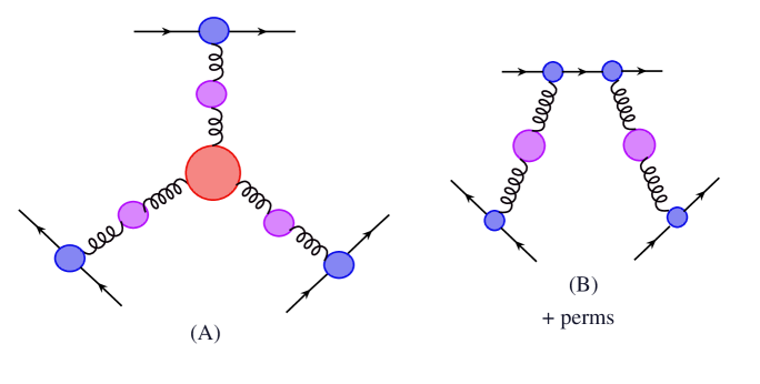
Figure 2: The tree-level skeleton graphs dressed with pinch-technique vertices and self-energies, which are used to define effective charges both for the quark-quark-gluon vertex (depending on a single gluon virtuality) and for the three-gluon vertex, which depends on three different momenta.

Generically the amplitude of the three-gluon graph can be written

$${\cal M}={\cal C}g_{0}^{4}V_{1}^{\nu_{1}}V_{2}^{\nu_{2}}V_{3}^{\nu_{3}}D_{\mu_{1}\nu_{1}}(k_{1})D_{\mu_{2}\nu_{2}}(k_{2})D_{\mu_{3}\nu_{3}}(k_{3})\Gamma_{\mu_{1}\mu_{2}\mu_{3}}(k_{1},k_{2},k_{3}),$$ (112)

where ${\cal C}$ is the overall color factor and $g_{0}$ is the bare coupling. The PT vertices $V_{i}$ are for gluons coupled to external particles, whose indices are suppressed; this is shown in Fig. 2 for external quarks. $\Gamma=\sum_{i=1}^{13}F_{i}\hat{f}_{i}$ is the gauge invariant three gluon vertex, whose thirteen form factors ($F_{i}$) are given in the preceding section. Finally the “gauge invariant” PT gluon propagator is

$$D_{\mu\nu}(k) = {1\over k^{2}}\left({t_{\mu\nu}(k)\over 1+\Pi(k^{2})}+\xi l_{\mu\nu}(k)\right)$$

$$t_{\mu\nu}(k) = \left\{\begin{array}[]{ccc}g_{\mu\nu}-{k_{\mu}k_{\nu}\over k^{2}}\\ g_{\mu\nu}-{n_{\mu}k_{\nu}+k_{\mu}n_{\nu}\over n\cdot k}\end{array}\right\}{\rm in}\left\{\begin{array}[]{ccc}{\rm covariant}\\ {\rm axial}\end{array}\right\}{\rm gauges}$$ (117)

$$l_{\mu\nu}(k) = \left\{\begin{array}[]{ccc}{k_{\mu}k_{\nu}\over k^{2}}\\ {k_{\mu}k_{\nu}\over(n\cdot k)^{2}}\end{array}\right\}{\rm in}\left\{\begin{array}[]{ccc}{\rm covariant}\\ {\rm axial}\end{array}\right\}{\rm gauges},$$ (122)

where $\xi$ is the gauge fixing parameter. This is “gauge invariant” in the maximal sense, i.e. the gauge dependence comes only from the tree level terms, and in particular $\Pi(k^{2})$ is totally gauge invariant.

Regardless of whether the external particles are quarks, gluons, or scalars, the vertices satisfy $k_{1}^{\mu}V_{1,\mu}=0$ when these particles are on shell (OS). One can then show that the gauge dependent terms coming from Eq.(4) vanish in the full amplitude consisting of all of the graphs in Fig.(2). This can be seen trivially in the covariant gauges where the gauge cancelations occur graph by graph, and with some work in axial gauges, where the cancelation occurs between all of the graphs. In the latter case, one must use the fact that the three gluon vertex satisfies the Ward ID in Eq.(3). Therefore we can take

$$D_{\mu\nu}(k)\rightarrow{g_{\mu\nu}\over k^{2}(1+\Pi(k^{2}))}.$$ (123)

Also, in the $\pm$ basis (Eq.(2.2)) any tensor with a ${}^{\prime}+^{\prime}$ in any slot gives vanishing contribution to ${\cal M}$. For example, $(+00)=(k_{2}+k_{3})_{\mu_{1}}g_{\mu_{2}\mu_{3}}=-k_{1,\mu_{1}}g_{\mu_{2}\mu_{3}}$, and $k_{1,\mu_{1}}$ dots into $V_{1,\mu_{1}}$ yielding zero. Hence only $(00-),(-00),(0\!-\!0)$, and $(\!-\!-\!-\!)$ contribute, and we find

$${\cal M}={{\cal C}g_{0}^{3}\over(1+\Pi(k_{1}^{2}))(1+\Pi(k_{2}^{2}))(1+\Pi(k_{3}^{2}))}{V_{1}^{\mu_{1}}V_{2}^{\mu_{2}}V_{3}^{\mu_{3}}\over k_{1}^{2}k_{2}^{2}k_{3}^{2}}g_{0}\Gamma_{\mu_{1}\mu_{2}\mu_{3}}^{OS}(k_{1},k_{2},k_{3}),$$ (124)

where the three-gluon vertex connected to on-shell (OS) external particles is

$$\Gamma_{\mu_{1}\mu_{2}\mu_{3}}^{OS}(k_{1},k_{2},k_{3})=(1+A_{0})\hat{a}_{0}+A_{+}\hat{a}_{+}+A_{-}\hat{a}_{-}+H\hat{h},$$ (125)

in the notation of section 2 where hatted objects are three index basis tensors.

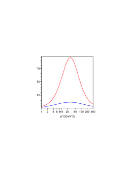
Figure 3: The effective scale $Q^{2}_{eff}(10\;{\rm GeV}^{2},10\;{\rm GeV}^{2},p^{2})$ is the lower blue curve, while $Q^{2}_{eff}(-10\;{\rm GeV}^{2},-10\;{\rm GeV}^{2},p^{2})=Q^{2}_{eff}(10\;{\rm GeV}^{2},10\;{\rm GeV}^{2},-p^{2})$ is the upper red curve. These both asymptote to zero, although very slowly for the upper curve.

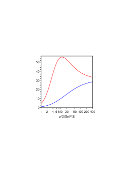
Figure 4: The effective scale $Q^{2}_{eff}(10\;{\rm GeV}^{2},p^{2},p^{2})$ is the lower blue curve, while $Q^{2}_{eff}(-10\;{\rm GeV}^{2},p^{2},p^{2})=Q^{2}_{eff}(10\;{\rm GeV}^{2},-p^{2},-p^{2})$ is the upper red curve. These both asymptote to $10e^{\Omega}\;{\rm GeV^{2}}\approx 31.25\;{\rm GeV^{2}}$.

Now one naturally defines PT effective charges by

$$g^{2}(k_{i}^{2})\equiv{g_{0}^{2}\over 1+\Pi(k_{i}^{2})}\;\;\;\;i=1,2,3.$$ (126)

Since we only have a single power of $g_{0}$ for each $1/(1+\Pi(k_{i}^{2}))$, this leaves $\prod_{i=1}^{3}{1/\sqrt{1+\Pi(k_{i}^{2})}}\approx 1-{\litfont{1\over 2}}(\Pi(k_{1}^{2})+\Pi(k_{2}^{2})+\Pi(k_{3}^{2}))$ to be absorbed into the three gluon vertex. Thus we have

$$\prod_{i=1}^{3}{1\over\sqrt{1+\Pi(k_{i}^{2})}}\Gamma_{\mu_{1}\mu_{2}\mu_{3}}^{OS}(k_{1},k_{2},k_{3}) = (1+\widetilde{A}_{0})\hat{a}_{0}+A_{+}\hat{a}_{+}+A_{-}\hat{a}_{-}+H\hat{h}$$

$$\widetilde{A}_{0}(k_{1}^{2},k_{2}^{2},k_{3}^{2})\equiv A_{0}(k_{1}^{2},k_{2}^{2},k_{3}^{2})\!\!\! - \!\!\!{\litfont{1\over 2}}\big{(}\Pi(k_{1}^{2})+\Pi(k_{2}^{2})+\Pi(k_{3}^{2})\big{)}$$ (127)

and

$${\cal M}={\cal C}g(k_{1}^{2})g(k_{2}^{2})g(k_{3}^{2}){V_{1}^{\mu_{1}}V_{2}^{\mu_{2}}V_{3}^{\mu_{3}}\over k_{1}^{2}k_{2}^{2}k_{3}^{2}}g_{0}\Big{[}(1+\widetilde{A}_{0})\hat{a}_{0}+A_{+}\hat{a}_{+}+A_{-}\hat{a}_{-}+H\hat{h}\Big{]}.$$ (128)

This naturally leads to the effective coupling of the three gluon vertex

$$\widetilde{g}(k_{1}^{2},k_{2}^{2},k_{3}^{2}) \equiv g_{0}(1+\widetilde{A}_{0}(k_{1}^{2},k_{2}^{2},k_{3}^{2}))$$

$$\widetilde{\alpha}(a,b,c) \equiv {\widetilde{g}^{2}(a,b,c)\over 4\pi}\approx{\alpha_{0}\over 1-2\widetilde{A}_{0}(a,b,c)},$$ (129)

first obtained by Lu in [38]. Our amplitude then takes the final form

$${\cal M}={\cal C}g(k_{1}^{2})g(k_{2}^{2})g(k_{3}^{2})\widetilde{g}(k_{1}^{2},k_{2}^{2},k_{3}^{2}){V_{1}^{\mu_{1}}V_{2}^{\mu_{2}}V_{3}^{\mu_{3}}\over k_{1}^{2}k_{2}^{2}k_{3}^{2}}\Big{[}\hat{a}_{0}+A_{+}\hat{a}_{+}+A_{-}\hat{a}_{-}+H\hat{h}\Big{]}.$$ (130)

Recall from the previous section that $A_{\pm},H\propto N_{c}-N_{f}$ in QCD.

The three-gluon effective coupling evolves according to

$$\widetilde{\alpha}(a,b,c)={\widetilde{\alpha}(a_{0},b_{0},c_{0})\over 1-2\Big{(}\widetilde{A}_{0}(a,b,c)-\widetilde{A}_{0}(a_{0},b_{0},c_{0})\Big{)}}$$ (131)

In four dimensions with regularization scheme $R=DRED\;{\rm or}\;DREG$ we have

$$\widetilde{A}_{0}(a,b,c) = -{\alpha_{s}\over 8\pi}\beta_{0}\Big{[}L(a,b,c)-\log{\mu^{2}}-C_{UV}-\eta_{3}\Big{]}$$

$${\rm where}\;\;\beta_{0} = {11\over 3}N_{c}-{2\over 3}N_{f}-{1\over 6}N_{s}$$

$$C_{UV} = {1\over\epsilon}-\gamma_{E}+\log{4\pi}$$ (132)

$$\eta_{3} = (2+\Omega)+{N_{c}\over 3\beta_{0}}\delta_{R,DREG}$$

$$\Omega = {16\over 3\sqrt{3}}{\rm Cl}_{2}(\pi/3)\approx 3.125$$

The scheme dependence $\delta_{R,DREG}$ is explained in more detail in Appendix D. Here we have defined

$$L(a,b,c)={1\over{\cal K}}\Big{(}\alpha\gamma\log{a}+\alpha\beta\log{b}+\beta\gamma\log{c}-abc\overline{J}(a,b,c)\Big{)}+\Omega,$$ (133)

and the (massless) triangle integral function $\overline{J}=\overline{J}(a,b,c)=-16i\pi^{2}J(a,b,c)$ is given in Appendix B in terms of Clausen functions, Eqs.(• ‣ 6,• ‣ 6). This result (Eqs.(4,4)) differs from Lu [38] by only the finite constants which (slightly) affects the numerical extraction from data. The discrepancy can be traced to the inconsistent application of dimensional regularization in [38].

The logarithm-like function $L$ satisfies

$$L(a,a,a)=\log{a}$$ (134)

since

$$\overline{J}(a,a,a)={4\over a\sqrt{3}}{\rm Cl}_{2}(\pi/3).$$ (135)

One can use the real part of this function to define an effective scale of the three-gluon vertex:

$$L(a,b,c) = \log{\left(Q_{eff}^{2}(a,b,c)\right)}+i{\rm Im~{}}L(a,b,c)$$

$$Q_{eff}^{2}(a,b,c) = |a|^{\alpha\gamma/{\cal K}}|b|^{\alpha\beta/{\cal K}}|c|^{\beta\gamma/{\cal K}}\exp{\Big{(}\Omega-{abc\over{\cal K}}{\rm Re~{}}\overline{J}(a,b,c)\Big{)}}.$$ (136)

This is sensible since the dimensions of $Q_{eff}^{2}(a,b,c)$ are indeed mass squared.

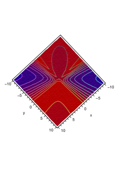
Figure 5: A contour plot of $Q^{2}_{eff}(1,x,y)$. The contours, from red to blue, are at $2,4,6,8,10,12,14,16,18,20$.

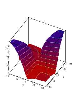
Figure 6: A three-dimensional contour plot of $Q^{2}_{eff}(1,x,y)$.

The three gluon effective charge $\widetilde{\alpha}(a,b,c)$ is related to the usual $\overline{MS}$ coupling $\overline{\alpha}(q^{2})$ by

$${1\over\widetilde{\alpha}(a,b,c)} = {1\over\overline{\alpha}(\mu^{2})}+{\beta_{0}\over 4\pi}\Big{(}\log{Q_{eff}^{2}(a,b,c)\over\mu^{2}}+i{\rm Im~{}}{L(a,b,c)}-\eta_{3}\Big{)}$$ (137)

$$= {1\over\overline{\alpha}(e^{-\eta_{3}}Q_{eff}^{2}(a,b,c))}+i{\beta_{0}\over 4\pi}{\rm Im~{}}{L(a,b,c)}.$$

Since $\exp{\left(\eta_{3}\over 2\right)}\approx 14$, we see that when using $\overline{MS}$, the scale should be fourteen times lower than the typical virtualities of the gluons, given by $Q_{eff}(a,b,c)$. Of course, this is true only if the three-gluon vertex diagram dominates the physical process. In general there will be different scales at the various quark-gluon vertices when using the PT scheme (as seen in Eq.(130)). In contrast, in $\overline{MS}$ the same scale is used at every vertex. The following approximate values of the three-gluon coupling are derived from Eq.(137) (including the effects of quark masses which discussed in the next section) for various symmetric timelike(T) and spacelike(S) configurations :

$$\begin{array}[]{ll}{\rm SSS}:&\widetilde{\alpha}(-M_{Z}^{2},-M_{Z}^{2},-M_{Z}^{2})\approx 0.192\\ {\rm SST}:&\widetilde{\alpha}(-M_{Z}^{2},-M_{Z}^{2},+M_{Z}^{2})\approx 0.157+0.023I\\ {\rm STT}:&\widetilde{\alpha}(-M_{Z}^{2},+M_{Z}^{2},+M_{Z}^{2})\approx 0.156+0.025I\\ {\rm TTT}:&\widetilde{\alpha}(+M_{Z}^{2},+M_{Z}^{2},+M_{Z}^{2})\approx 0.170+0.062I\end{array}$$

It is clear that the three-gluon coupling is stronger than naively expected from $\alpha_{\overline{MS}}(M_{Z})\approx 0.118$.

The effective scale $Q_{eff}^{2}(a,b,c)$ satisfies the following relations:

$$Q_{eff}^{2}(a,b,c) = Q_{eff}^{2}(-a,-b,-c)$$

$$Q_{eff}^{2}(\lambda a,\lambda b,\lambda c) = |\lambda|Q_{eff}^{2}(a,b,c)$$

$$Q_{eff}^{2}(a,a,a) = |a|$$ (138)

$$Q_{eff}^{2}(a,-a,-a) \approx 5.54|a|$$

$$Q_{eff}^{2}(a,a,c) {\approx} |c|e^{\Omega-2}\;\;\;\;\;\;\;{\rm for}\;\;|a|\gg|c|$$

$$Q_{eff}^{2}(a,-a,c) {\approx} |c|e^{\Omega}\;\;\;\;\;\;\;{\rm for}\;\;|a|\gg|c|$$

$$Q_{eff}^{2}(a,b,c) {\approx} {|b||c|\over|a|}e^{\Omega}\;\;\;\;\;\;\;{\rm for}\;\;|a|\gg|b|,|c|.$$

Lu [38] has previously found the last of these limits in the case where all momenta are spacelike, giving an effective scale $Q_{min}Q_{med}/Q_{max}$. It should be noted that the rate of convergence to the above limits strongly depends on the signatures (${\rm S}\equiv{\rm spacelike}\leftrightarrow p^{2}<0$, ${\rm T}\equiv{\rm timelike}\leftrightarrow p^{2}>0$) of the virtualities $a,b,c$. If the signatures are mixed (TTS) or (TSS) then the convergence is very slow, and the effective scale tends to stay larger compared to the cases (SSS) or (TTT).

Some plots demonstrating the novel behavior of $Q_{eff}^{2}$ are given in Figs.(3,4,5,6).

5 Phenomenological Effects of Internal Masses

So far, all fields propagating in the triangle graphs have been treated as massless. This was useful for simplifying the discussion and elucidating the general structure of the radiative corrections and the $N=4$ sum rules. However, in real world applications one usually does not have all three gluon virtualities in the same desert region $M_{i}\ll a,b,c\ll M_{i+1}$. Thus, mass corrections should be taken into account. We have calculated the effects of massive fermions (MQ), massive scalars (MS), and massive gauge bosons (MG) for all of the form factors; the complete results are given in Appendix E. The corrections for the case of massive fermions were first obtained in Ref.[39] and we are in agreement. Here we will focus on the massive quark ($MQ$) contribution to the form factor multiplying the tree level tensor structure, which from Appendix E and section 3 is

$$A_{0}(MQ)={4M^{2}\over 3(d-2)}J_{M}+{3d-8\over 6{\cal K}(d-2)}\Big{[}abcJ_{M}+a\beta J_{1M}+b\gamma J_{2M}+c\alpha J_{3M}\Big{]}.$$ (139)

Here $J_{M}$, $J_{1M}$, $J_{2M}$, and $J_{3M}$ are the massive analogs of $J,J_{1},J_{2}$ and $J_{3}$, respectively. The two-point function $J_{1M}$ and tadpole $T_{M}$ are reviewed in Appendix A, while Appendix B is devoted to a discussion of the massive triangle integral, $J_{M}$, and its analytic continuations and various limits.

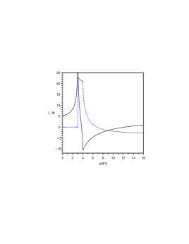
Figure 7: $L_{MQ}(a/M^{2},a/M^{2},a/M^{2})$ vs. $a/M^{2}$ for timelike $a>0$. The solid line is the real part and the dashed line is the imaginary part.

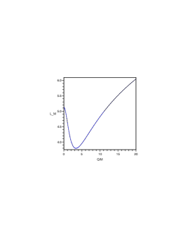
Figure 8: $L_{MQ}(-Q^{2}/M^{2},-Q^{2}/M^{2},-Q^{2}/M^{2})$ vs. $Q/M$ for spacelike $-Q^{2}<0$.

As in the previous section, when considering a physical matrix element we always have the combination $\widetilde{A}_{0}=A_{0}-{\litfont{1\over 2}}\big{(}\Pi_{1}+\Pi_{2}+\Pi_{3}\big{)}$ multiplying the tree-level tensor structure. This leads us to consider the massive quark contribution $\widetilde{A}_{0}(MQ)=A_{0}(MQ)-{\litfont{1\over 2}}\big{(}\Pi_{1}(MQ)+\Pi_{2}(MQ)+\Pi_{3}(MQ)\big{)}$, which upon using Eq.(6), inserting the prefactor $ig^{2}$, and expanding around $d=4$ becomes

$$\widetilde{A}_{0}(MQ) = -{\alpha_{s}\over 4\pi}\Bigg{[}{1\over 3}\left(C_{UV}-\log{M^{2}\over\mu^{2}}\right)+{2\over 3}+{1\over 3{\cal K}}\left(abc\overline{J_{M}}-\alpha\gamma{\cal L}(a)-\alpha\beta{\cal L}(b)-\beta\gamma{\cal L}(c)\right)$$ (140)

$$+ {2M^{2}\over 3}\left(\overline{J_{M}}+{2-{\cal L}(a)\over a}+{2-{\cal L}(b)\over b}+{2-{\cal L}(c)\over c}\right)\Bigg{]}.$$

Here $\overline{J_{M}}=-16i\pi^{2}J_{M}$ and

$${\cal L}(a)=v(a)\log{v(a)+1\over v(a)-1}\;\;{\rm where}\;\;v(a)=\sqrt{1-{4(M^{2}-i\epsilon)\over a}},$$ (141)

comes from $J_{1M}$ and has the analytic continuations given in Eq.(179). The three-scale logarithm-like function for massive quarks (MQ) is thus given by

$$L_{MQ}\left({a\over M^{2}},{b\over M^{2}},{c\over M^{2}}\right) = {1\over{\cal K}}\Big{(}\alpha\gamma{\cal L}(a)+\alpha\beta{\cal L}(b)+\beta\gamma{\cal L}(c)-abc\overline{J_{M}}(a,b,c)\Big{)}+\Omega$$ (142)

$$+ 2M^{2}\left({{\cal L}(a)-2\over a}+{{\cal L}(b)-2\over b}+{{\cal L}(c)-2\over c}-\overline{J_{M}}\right)$$

$$\widetilde{A}_{0}(MQ) = \left({\alpha_{s}\over 12\pi}\right)\left[L_{M}\left({a\over M^{2}},{b\over M^{2}},{c\over M^{2}}\right)+\log{M^{2}\over\mu^{2}}-C_{UV}-(2+\Omega)\right].$$

This massive logarithm-like function has the following limits :

$$L_{MQ}\left({a\over M^{2}},{b\over M^{2}},{c\over M^{2}}\right) \approx 2+\Omega\;\;\;\;\;\;\;\;\;\;\;\;\;\;\;\;\;\;\;\;\;\;M^{2}\gg|a|,|b|,|c|$$

$$L_{MQ}\left({a\over M^{2}},{b\over M^{2}},{c\over M^{2}}\right) \approx L(a,b,c)-\log{M^{2}}\;\;\;\;\;\;\;M^{2}\ll|a|,|b|,|c|,$$ (143)

with the number $\Omega\approx 3.125$ defined in Eq.(4). The convergence to the massless limit is very slow, indicating that threshold effects must be included for most applications.

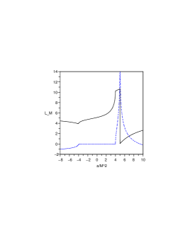
Figure 9: $L_{MQ}(a/M^{2},a/M^{2},-a/M^{2})$ vs. $a/M^{2}$. The solid line is the real part and the dashed line is the imaginary part. The real thresholds are at $a=\pm 4M^{2}$ while the pseudo-threshold is at $a=5M^{2}$.

In Figs.(7,8) we have plotted $L_{MQ}$ for the symmetric case $a=b=c$ for timelike and spacelike momenta. For the timelike case, the threshold at $a=4M^{2}$ and the pseudo-threshold at $a=3M^{2}$ are evident. In Fig.(9) the mixed case (TTS) $L_{MQ}(a/M^{2},a/M^{2},-a/M^{2})$ is plotted, where the thresholds at $a=\pm 4M^{2}$ and the pseudo-threshold at $a=5M^{2}$ are evident. For the purely timelike (TTT) case in Fig.(7), there is a discontinuity in the imaginary part and the real part diverges at the pseudo-threshold. In contrast, for the mixed signature case (TTS) the imaginary part diverges while the real part is discontinuous. This pseudo-threshold phenomena is explained in more detail in Appendix B.

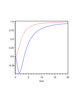
Figure 10: The effective number of quark flavors. The lower blue solid curve is $N_{F}(Q^{2}/M^{2})$ for the symmetric spacelike ($a=b=c=-Q^{2}$) three-gluon vertex, while the upper dashed red curve is the fermion number of flavors $N_{1/2}(Q^{2}/M^{2})$ for the single scale effective charge.

From the above results, one can define the effective number of active quarks which characterizes the effects of quark mass :

$$N_{F}\left({a\over M^{2}},{b\over M^{2}},{c\over M^{2}}\right)=-M^{2}{d\over dM^{2}}L_{MQ}\left({a\over M^{2}},{b\over M^{2}},{c\over M^{2}}\right).$$ (144)

This clearly goes to zero and one in the limits $M^{2}\gg|a|,|b|,|c|$ and $M^{2}\ll|a|,|b|,|c|$, respectively.

To motivate this definition, let’s look at the single-scale pinch-technique effective charge (using the notation of [13]) as a function of spacelike momenta $a=-Q^{2}$

$${1\over\widetilde{\alpha}(Q^{2})}={1\over\alpha_{0}}+{1\over 4\pi}\sum_{p}\beta_{p}\left(L_{p}(Q^{2}/m_{p}^{2})-\log{\mu^{2}\over m_{p}^{2}}-C_{UV}-\eta_{p}\right),$$ (145)

where $\beta_{p}$ is the contribution of each particle $p$ to the first $\beta$ function coefficient, and to a very good numerical approximation (for spacelike momenta)

$$L_{p}(Q^{2}/m_{p}^{2})\approx\log{\left(e^{\eta_{p}}+{Q^{2}\over m_{p}^{2}}\right)},$$ (146)

where the constants $\eta_{p}$ are $5/3,8/3,$ and $40/21$ for massive fermions, scalars, and gauge bosons, respectively. The exact one-loop formula are given in Eq.(23-26) of Ref.[13], although the analytic continuation in Eq.(26) of that paper should have opposite imaginary part. This effective charge satisfies the RGE

$${d\widetilde{\alpha}(Q^{2})\over d\log{Q^{2}}} = -{\widetilde{\alpha}^{2}\over 4\pi}\sum_{p}\beta_{p}{dL_{p}(Q^{2}/m_{p}^{2})\over d\log{Q^{2}}}\equiv-{\widetilde{\alpha}^{2}\over 4\pi}\sum_{p}\beta_{p}N_{p}\left({Q^{2}\over m_{p}^{2}}\right)$$

$$N_{p}\left({Q^{2}\over m_{p}^{2}}\right) \equiv {dL_{p}(Q^{2}/m_{p}^{2})\over d\log{Q^{2}}}=-{dL_{p}(Q^{2}/m_{p}^{2})\over d\log{m_{p}^{2}}}\approx{1\over 1+{m_{p}^{2}\over Q^{2}}e^{\eta_{p}}}.$$ (147)

The function $N_{p}$ goes to one when $Q^{2}\gg m_{p}^{2}$ and zero when $Q^{2}\ll m_{p}^{2}$ and unambiguously measures what fraction of particle $p$ is “turned on” at scale $Q^{2}$.

Moving back to the three-scale case, we now have the complication that our effective charge is a solution of a multi-scale RGE

$${d\widetilde{\alpha}(a,b,c)\over d\log{a}}=-{\widetilde{\alpha}^{2}\over 4\pi}\sum_{p}\beta_{p}{d\over d\log{a}}L_{MQ}\left({a\over M^{2}},{b\over M^{2}},{c\over M^{2}}\right),$$ (148)

and two other permutations with $a\rightarrow b$ or $a\rightarrow c$. This leads to three different $N_{f}$’s :

$$N_{f}\left({a\over M^{2}}\Big{|}{b\over M^{2}},{c\over M^{2}}\right)={d\over d\log{a}}L_{MQ}\left({a\over M^{2}},{b\over M^{2}},{c\over M^{2}}\right),$$ (149)

and two cyclic permutations, each of which goes to $1/3$ in the symmetric desert $a=b=c\gg M^{2}$. This suggests adding all three together to define a symmetric

$$N_{F}\left({a\over M^{2}},{b\over M^{2}},{c\over M^{2}}\right)=\left({d\over d\log{a}}+{d\over d\log{b}}+{d\over d\log{c}}\right)L_{MQ}\left({a\over M^{2}},{b\over M^{2}},{c\over M^{2}}\right),$$ (150)

which is in fact the same as given in Eq.(144).

The results for $N_{F}$ can be obtained with the help of the results in Appendix B. Instead of presenting these lengthy results, let us focus on the symmetric case $a=b=c$, where we find for spacelike $a<0$

$$N_{F}\left({a\over M^{2}}\right) \equiv {d\over d\log{a}}L_{MQ}\left({a\over M^{2}},{a\over M^{2}},{a\over M^{2}}\right)=-{d\over d\log{M^{2}}}L_{MQ}\left({a\over M^{2}},{a\over M^{2}},{a\over M^{2}}\right)$$ (151)

$$= 1+18{M^{2}\over a}+2M^{2}\overline{J_{M}}(a,a,a)+54M^{2}{\cal L}(a){a-2M^{2}\over(a-3M^{2})(a-4M^{2})}.$$

In this example, spacelike $a$ is chosen to avoid the pseudo-threshold $a=3M^{2}$ and the threshold $a=4M^{2}$. Fig.(10) shows a plot of this along with single-scale quark number of flavors function $N_{s=1/2}$ from Eq.(5).

The negative value of $N_{F}$ at $0\mathrel{\mathstrut\smash{\ooalign{\raise 2.5pt\hbox{$<$}\cr\lower 2.5pt\hbox{$\sim$}}}}Q\mathrel{\mathstrut\smash{\ooalign{\raise 2.5pt\hbox{$<$}\cr\lower 2.5pt\hbox{$\sim$}}}}4M$ is not entirely novel, as a similar behavior was also found in the context of two-loop quark mass corrections to V-scheme effective charge [40]. It is essentially due to the anti-screening of color charge, this case in the triangle interaction, and does not arise in the one-loop single scale effective charge, as seen in Fig.(9).

Using the results of Appendix E, the above analysis can be easily extended to the case of massive scalars (MS) or massive gauge bosons (MG), which have the following logarithm-like functions

$$L_{MS}\left({a\over M^{2}},{b\over M^{2}},{c\over M^{2}}\right) = {1\over{\cal K}}\Big{(}\alpha\gamma{\cal L}(a)+\alpha\beta{\cal L}(b)+\beta\gamma{\cal L}(c)-abc\overline{J_{M}}(a,b,c)\Big{)}+\Omega$$ (152)

$$- 4M^{2}\left({{\cal L}(a)-2\over a}+{{\cal L}(b)-2\over b}+{{\cal L}(c)-2\over c}-\overline{J_{M}}\right)$$

$$L_{MG}\left({a\over M^{2}},{b\over M^{2}},{c\over M^{2}}\right) = {1\over{\cal K}}\Big{(}\alpha\gamma{\cal L}(a)+\alpha\beta{\cal L}(b)+\beta\gamma{\cal L}(c)-abc\overline{J_{M}}(a,b,c)\Big{)}+\Omega$$ (153)

$$+ {4\over 7}M^{2}\left({{\cal L}(a)-2\over a}+{{\cal L}(b)-2\over b}+{{\cal L}(c)-2\over c}-\overline{J_{M}}\right).$$

The qualitative behavior is the same as the quark case.

Finally, we should consider the limitations of the effective scale $Q^{2}_{eff}(a,b,c)$ introduced in the last section and effective number of flavors $N_{F}(a/M^{2},b/M^{2},c/M^{2})$ discussed in this section. Given the complicated structure of the full mass dependent form factors, such tools for characterizing and understanding the behavior of the vertex are helpful. However, in a real calculation such methods may be of limited use and the full mass dependent results should be used. For example, the effective scale $Q^{2}_{eff}$ has been defined only in the massless case so far because the definition becomes complicated and somewhat arbitrary in the massive case. In particular, consider the possible definition (for QCD):

$${\rm Re~{}} \!\!\!\Bigg{[}{11\over 3}C_{A}L(a,b,c)-{2\over 3}\sum_{q}\Bigg{(}L_{MQ}\left({a\over M_{q}^{2}},{b\over M_{q}^{2}},{c\over M_{q}^{2}}\right)+\log{M_{q}^{2}}\Bigg{)}\Bigg{]}$$ (154)

$$\equiv \Bigg{(}{11C_{A}\over 3}-{2\over 3}\sum_{q}\widetilde{N_{q}}\left({a\over M_{q}^{2}},{b\over M_{q}^{2}},{c\over M_{q}^{2}}\right)\Bigg{)}\log{\widetilde{Q}^{2}_{eff}(a,b,c)},$$

where $\widetilde{N_{q}}$ is some suitably defined number of flavors, possibly a step function such as $\delta(a+b+c-3M_{q}^{2})$, possibly the $N_{F}$ defined in Eq.(144), or some other definition. It should be clear that any choice of $\widetilde{N_{q}}$ determines $\widetilde{Q}_{eff}^{2}$, and vice versa, and there seems to be no compelling choice for these quantities. Furthermore, in the approach advocated here, the couplings at each vertex depend on physical momentum scales which will typically be integrated over in the phase space. Thus, matching onto a conventional $\overline{MS}$ type approach can only be done at the end of the calculation, so that trying to define a $Q_{eff}^{2}$ at an intermediate stage is not very useful.

Thus, in real world applications, one should generally use the full results for the mass dependent form factors. This constitutes a multi-scale analytic renormalization scheme that contains information which cannot be obtained in the simple single-scale leading-log renormalization methods. In other words, every three-gluon vertex (at tree-level) can be dressed, or “RG improved”, with this gauge-invariant effective coupling and the associated form factors, which are process independent and contain more information than the $\overline{MS}$ procedure.

6 Conclusions and Future Directions

The results of this paper represent only a fraction of what is needed for a re-organization of perturbation theory into fully gauge-invariant pieces with physical content, each of which can be renormalized independently, leading naturally to a physical multi-scale analytic renormalization scheme. This is possible due to the remarkable properties of the pinch technique (PT)/ Background Field Method quantum Feynman gauge (BFMFG) Green’s functions. There is still much progress that can be made in calculating these Green’s functions in perturbation theory.

The present paper gives a complete and general characterization of the off-shell three-gluon vertex at one-loop. A similar study of the gauge-invariant triple gauge boson vertices of the Standard Model [14] would be very useful. It may also be possible to quantitatively look at the unification of triple gauge boson vertices and couplings, in analogy with the work on the unification of single-scale PT couplings[13]. Some progress has been made on the conventional gauge-dependent three-gluon vertex at two loops [41][42], which gives hope for eventually treating the gauge-invariant three-gluon vertex at two-loops.

The gauge boson two-point functions and the associated effective charges for QCD [2][5], electroweak theory [15][8][11], and supersymmetric grand unified models [13] have been calculated in the past to one-loop. We know from general principles the divergent parts at two-loops, but no complete two-loop PT calculation as yet exists. To fill this gap, the two-loop gluon PT self-energy will be presented in the near future [37]. This will allow for a more precise determination of coupling from data, as well as giving the three-loop $\beta$ function coefficient. Furthermore, by the Ward identity in Eq.(3), this also yields the longitudinal form factors of $\Gamma_{\mu_{1}\mu_{2}\mu_{3}}^{(ggg)}$ through two loops.

The gauge-invariant PT/BFMFG quark self-energy turns out to be equal to the conventional self-energy in the Feynman gauge [25], and so is known through two-loops [43]. Due to the Ward identity [24] satisfied by the PT/BFMFG quark-gluon vertex, this also yields the longitudinal form factors of $\Gamma_{\mu}^{(qqg)}$ through two loops.

In QCD, another logical step is the four-gluon vertex at one-loop. In the general off-shell case, there are hundreds of independent tensors structures and form factors.

Beyond perturbation theory, the study of Dyson-Schwinger Equations [3] and renormalons [7] in the PT/BFMFG approach may yield new insight.

To summarize, in this paper we have analyzed the behavior of the gauge-invariant three-gluon vertex at one-loop. Starting from the symmetry principles governing the vertex, a convenient tensor basis decomposition was given in Eqs.(2.2,50). As seen in Eq.(125) and the subsequent discussion, this basis is the most convenient for phenomenological studies, since it is built out of “transverse” ($-$) and “longitudinal” ($+$) momenta, the latter of which vanish when dotted into external on-shell vertices, thus leading to relatively simple matrix elements. In the case considered in section 4, only four form factors remain, rather than the thirteen which would be present in a generic basis. Nonetheless, the choice of basis is only a matter of convenience, and the real physics lies in the thirteen non-vanishing form factors given explicitly in section 3.

The supersymmetric relations between the scalar, quark, and gluon contributions leads to a simple presentation of the results for a generic (unbroken) gauge theory. Only the gluon contributions to the form factors are given explicitly in section 3, while the quark and scalar contributions are inferred from the homogeneous relation $F_{G}+4F_{Q}+(10-d)F_{S}=0$ and the results for the relatively simple sums $\Sigma_{QG}(F)\equiv{(d-2)\over 2}F_{Q}+F_{G}$ which are given in section 3 for each form factor $F$. The extension to the case of internal masses is outlined in Appendix E and leads to the modified sum rule $F_{MG}+4F_{MQ}+(9-d)F_{MS}=0$.

The phenomenology is largely determined by the form factor of the tree-level tensor structure, which in section 4 is used to define a three-scale effective charge $\widetilde{\alpha}(a,b,c)$. In addition, the characteristic scale $Q^{2}_{eff}(a,b,c)$ governing the behavior of the vertex and the effective charge was analyzed, thus providing a natural extension of BLM scale setting [44] to the three-gluon vertex. Physical momentum scales always set the scale of the coupling. The phenomenological effects of quark masses are discussed in section 5 and are found to be important for generic physical applications, since decoupling is slow and a complicated threshold and pseudo-threshold behavior is observed. An important next step is to fully apply these techniques to a physical process. In the future we will present such an analysis for the hadronic production of heavy quarks, where the importance of the form factors other than the tree-level one ($A_{0}$) will be addressed. The interpretation of the pseudo-threshold phenomena also deserves further study.

Acknowledgements M.B. would like to thank Lance Dixon for useful discussions regarding the second order formalism of the BFM and the supersymmetric decomposition of one-loop amplitudes.

Appendix A: Reduction to Scalar Integrals

First, we will describe the evaluation of the massless integrals, and then briefly mention the modifications due to internal masses. As before, we will use the shorthand notation

$$a=p_{1}^{2}\;\;\;\;\;b=p_{2}^{2}\;\;\;\;\;c=p_{3}^{2}\;\;\;\;\;\alpha=p_{1}\!\cdot\!p_{2}\;\;\;\;\;\beta=p_{2}\!\cdot\!p_{3}\;\;\;\;\;\gamma=p_{3}\!\cdot\!p_{1}$$ (155)

In order to evaluate the integrals in an efficient manner, it is very convenient to choose a manifestly symmetric routing of the loop momenta, as shown in Fig.1, where clearly

$$l_{1}=p_{2}+l_{3}\;\;\;\;l_{2}=p_{3}+l_{1}\;\;\;\;l_{3}=p_{1}+l_{2}.$$ (156)

Of course there is only one integration momenta $l$, which can be chosen to be $l_{1},l_{2},$ or $l_{3}$, thus breaking the cyclic symmetry. However, using the symmetric labeling greatly simplifies the analysis.

First we decompose the full vertex $\Gamma$ into longitudinal ($L$) and transverse ($T$) parts, $\Gamma=\Gamma_{L}+\Gamma_{T}$, as in Eq.(2.2). The tensor integrals in Eq.(3) are then converted into scalar integrals by applying projection operators. In doing so, the longitudinal ($L$) and transverse ($T$) parts essentially decouple, and the ten independent $L$ form factors are easily found either directly, or by solving the Ward ID, resulting in Eq.(3.2). The remaining four $T$ parts are found by applying the following four projection operators to Eq.(3) : $200,030,001,$ and $231$, where as in Table 1 we have defined $030\equiv p_{3\mu_{2}}g_{\mu_{1}\mu_{3}}$, etc. Thus, for the gluon contribution $G$ we have four scalar integrals : $G(200)\equiv p_{2\mu_{1}}g_{\mu_{2}\mu_{3}}G_{\mu_{1}\mu_{2}\mu_{3}},G(030),G(001),$ and $G(231)$. Similarly, there are four integrals for the quarks and scalars as well. In the numerator of each of these integrals there will be various dot products of momenta, which can always be reduced to momentum squares using Eq.(156). For example, $p_{1}\!\cdot\!l_{2}=(l_{3}^{2}-l_{2}^{2}-p_{1}^{2})/2$ and $l_{1}\!\cdot\!l_{3}=(l_{1}^{2}+l_{3}^{2}-p_{2}^{2})/2$. Thus we are left with integrals of the form

$$I_{ijk}=\int{(l_{1}^{2})^{i}(l_{2}^{2})^{j}(l_{3}^{2})^{k}\over l_{1}^{2}l_{2}^{2}l_{3}^{2}},$$ (157)

where $\int\equiv\int{d^{d}l\over(2\pi)^{d}}$ and $i,j,k\in\{0,1,2\}$. Using the standard rules of dimensional regularization, it is easy to see that any integral with any two of $i,j,k$ nonzero must vanish. Furthermore, it is straightforward to show that

$$I_{200}=-\beta I_{100}\;\;\;\;\;I_{020}=-\gamma I_{010}\;\;\;\;\;I_{002}=-\alpha I_{001}.$$ (158)

Thus we are left with only two types of integrals: (1) the trivial two point integrals $J_{1}$, $J_{2}$, and $J_{3}$, where

$$J_{1}=I_{100}=\int{1\over l_{2}^{2}l_{3}^{2}}=\int{1\over l^{2}(l+p_{1})^{2}},$$ (159)

and (2) the master triangle integral

$$J\equiv J(p_{1}^{2},p_{2}^{2},p_{3}^{2})=\int{1\over l_{1}^{2}l_{2}^{2}l_{3}^{2}}.$$ (160)

For the gluon contribution, for example, one then has a system of four equations with four unknowns, the transverse form factors. Denoting the gluon contribution to the longitudinal projections by $L_{G}(200)=200\cdot\Gamma_{L}(G)$, etc. we solve for the transverse form factors

$$\left(\begin{array}[]{cccc}\overline{F}_{12}(G)\\ \overline{F}_{23}(G)\\ \overline{F}_{31}(G)\\ \overline{H}(G)\end{array}\right) = M_{T}^{-1}\left(\begin{array}[]{cccc}G(200)-L_{G}(200)\\ G(030)-L_{G}(030)\\ G(001)-L_{G}(001)\\ G(231)-L_{G}(231)\end{array}\right)$$ (169)

$${\rm where}\;\;\;\;\;M_{T} = -{\cal K}\left(\begin{array}[]{cccc}\beta&(d-1)\beta&\beta&2-d\\ \gamma&\gamma&(d-1)\gamma&2-d\\ (d-1)\alpha&\alpha&\alpha&2-d\\ {\cal K}&{\cal K}&{\cal K}&0\end{array}\right),$$ (174)

and similarly for the quark and scalar contributions.

The above procedure can also be followed for the massive case, with only a few modifications. First, the tadpole $M^{2}T_{M}=\int{1\over l_{i}^{2}-M^{2}}$ does not vanish. Thus, instead of $\int{l_{1}^{2}\over l_{2}^{2}l_{3}^{2}}=-\beta J_{1}$ we now have

$$\int{l_{1}^{2}-M^{2}\over(l_{2}^{2}-M^{2})(l_{3}^{2}-M^{2})}=-\beta J_{1M}+M^{2}T_{M},$$ (175)

where $J_{1M}=\int{1\over(l_{2}^{2}-M^{2})(l_{3}^{2}-M^{2})}=\int{1\over(l^{2}-M^{2})((l+p_{1})^{2}-M^{2})}$. We also need the following result and permutations :

$$\int{l_{2}^{2}-M^{2}\over l_{3}^{2}-M^{2}}=\int{l_{3}^{2}-M^{2}\over l_{2}^{2}-M^{2}}=aM^{2}T_{M}.$$ (176)

Finally, we have the master triangle integral with nonzero masses

$$J_{M}\equiv J_{M}(p_{1}^{2},p_{2}^{2},p_{3}^{2})=\int{1\over(l_{1}^{2}-M^{2})(l_{2}^{2}-M^{2})(l_{3}^{2}-M^{2})}.$$ (177)

To summarize, in the massive case we need $J_{M}$, $J_{1M}$, $J_{2M}$, $J_{3M}$, and $T_{M}$. In the massless case we need $J$, $J_{1}$, $J_{2}$, and $J_{3}$. For each of these we pull out the factor ${i\over 16\pi^{2}}$ and define $J_{M}={i\over 16\pi^{2}}\overline{J_{M}}$, etc.

Some formula for these integrals in $d$ dimensions can be found in [35]. Here we will give only the expansions in four dimensions and define $C_{UV}={1\over\epsilon}-\gamma_{E}+\log{4\pi}$ where $d=4-2\epsilon$.

The tadpole integral is

$$\overline{T_{M}}=C_{UV}+1-\log{M^{2}\over\mu^{2}}.$$ (178)

The two point integral is

$$\overline{J_{1M}} = C_{UV}+2-\log{M^{2}\over\mu^{2}}-{\cal L}(a)$$ (179)

$${\cal L}(a) = \left\{\begin{array}[]{lll}2v\tanh^{-1}{(v^{-1})}=v\log{v+1\over v-1}\\ 2\overline{v}\tan^{-1}{(\overline{v}^{-1})}\\ 2v\tanh^{-1}{(v)}-i\pi v=v\log{1+v\over 1-v}-i\pi v\end{array}\right\}\;\;{\rm for}\;\;\left\{\begin{array}[]{lll}a<0\\ 0<a<4M^{2}\\ a>4M^{2}\end{array}\right\}$$ (186)

and the generalized velocities are

$$v=\sqrt{1-{4M^{2}\over a}}\;\;\;\;\;\;\;\;\;\;\;\;\overline{v}=\sqrt{{4M^{2}\over a}-1}.$$ (187)

In the massless limit this becomes

$$\overline{J_{1}}=C_{UV}+2-\log{|a|\over\mu^{2}}+i\pi\theta(a).$$ (188)

Appendix B: Results for the Triangle Integral

The massive triangle integral

$$J_{M}\equiv J_{M}(p_{1}^{2},p_{2}^{2},p_{3}^{2})=\int{d^{4}l\over(2\pi)^{4}}{1\over(l_{1}^{2}-M^{2}+i\epsilon)(l_{2}^{2}-M^{2}+i\epsilon)(l_{3}^{2}-M^{2}+i\epsilon)}$$ (189)

is finite in four dimensions. We will give the results for $\overline{J_{M}}=-i16\pi^{2}J_{M}$. This integral has been discussed previously in the literature [45][46][47][39]. In particular, ’tHooft and Veltman [45] derived a formula which is valid for all values of the kinematic variables $a,b,c$ and mass $M$, although careful analytic continuation is required. We will first write the results of [45] in our notation and then discuss the analytic continuations. The various functions involved and some reference formula are summarized below in Appendix C.

Defining $\rho=\sqrt{-{\cal K}}$, where as before

$${\cal K}=\alpha\beta+\beta\gamma+\gamma\alpha=-{1\over 4}\big{(}a^{2}+b^{2}+c^{2}-2(ab+bc+ca)\big{)},$$ (190)

we have

$$\overline{J_{M}}=-{1\over 2\rho}(I_{3}(a|b,c)+I_{3}(b|c,a)+I_{3}(c|a,b)).$$ (191)

The results for $I_{3}(a|b,c)$ can be expressed in terms of the velocity $v=\sqrt{1-{4(M^{2}-i\epsilon)\over a}}$ and the variable $x={\beta/\rho}$ :

$$I_{3}(a|b,c) = {\rm Li}_{2}(z_{1})-{\rm Li}_{2}(\overline{z_{1}})+{\rm Li}_{2}(z_{2})-{\rm Li}_{2}(\overline{z_{2}})-\eta(x-v,x+v)\log{\overline{z_{2}}\over z_{1}}$$ (192)

$$+ \eta(-1-v,{1\over x-v})\log{z_{1}}-\eta(1-v,{1\over x-v})\log{\overline{z_{2}}}$$

$$+ \eta(-1+v,{1\over x+v})\log{z_{2}}-\eta(1+v,{1\over x+v})\log{\overline{z_{1}}}$$

where we have defined

$$z_{1}={x+1\over x-v}\;\;\;z_{2}={x+1\over x+v}\;\;\;\overline{z_{1}}={x-1\over x+v}\;\;\;\overline{z_{2}}={x-1\over x-v}$$ (193)

and the function $\eta(x,y)$ compensates for the branch cut in the logarithms:

$$\log{xy} = \log{x}+\log{y}+\eta(x,y)$$ (194)

$$\eta(x,y) = 2i\pi\Big{(}\theta(-{\rm Im~{}}{x})\theta(-{\rm Im~{}}{y})\theta({\rm Im~{}}{x}{\rm Im~{}}{y})-\theta({\rm Im~{}}{x})\theta({\rm Im~{}}{y})\theta(-{\rm Im~{}}{x}{\rm Im~{}}{y})\Big{)}.$$

The other two integrals $I_{3}(b|c,a)$ and $I_{3}(c|a,b)$ are easily obtained by permutation of the above results, so that $x=\gamma/\rho,v=\sqrt{1-{4M^{2}\over b}}$ and $x=\alpha/\rho,v=\sqrt{1-{4M^{2}\over c}}$, respectively. Although these results entirely characterize the massive triangle function, it is a rather tedious exercise to analytically continue the results to the six different physical kinematical regions. To our knowledge, such complete analytic continuations have not appeared in the literature thus far.

$\overline{J_{M}}$ takes different forms for ${\cal K}>0$ and ${\cal K}<0$ since then the variable $x$ is imaginary and real, respectively. The case ${\cal K}>0$ can occur only if all momenta are spacelike $(a,b,c<0)$ or timelike $(a,b,c>0)$. The case ${\cal K}<0$ can occur for momenta of any signature. Thus, if all momenta are spacelike or all timelike, the ratios of momenta will determine if ${\cal K}>0$ or ${\cal K}<0$. For each of these two cases, we must also distinguish when $a$ is spacelike, timelike below threshold, and timelike above threshold. For timelike above threshold and spacelike, the generalized velocity $v=\sqrt{1-{4M^{2}\over a}}$ is real, except for the $i\epsilon$ term which is used in the analytic continuation and hence not included below. Below threshold $v=i\overline{v}=i\sqrt{{4M^{2}\over a}-1}$.

$\hskip 144.54pt{\rm\bf Case}\;\;\bf{{\cal K}>0}$

For ${\cal K}>0$ we have

$$\rho = \sqrt{-{\cal K}}\;=\;i\sqrt{{\cal K}}\;\equiv\;i\overline{\rho}$$

$$x = \beta/\rho\;=\;-i\beta/\overline{\rho}\;\equiv\;-iw$$ (195)

• ${\cal K}>0\;\;\;\;{\rm and}\;\;\;\;v\;{\rm real}\Longleftrightarrow(a<0\;{\rm or}\;a>4M^{2})$

  $$I_{3}(a|b,c) = i\Bigg{(}2{\rm Cl}_{2}(2\phi_{1})-{\rm Cl}_{2}(2\phi_{1}-2\phi_{2})-{\rm Cl}_{2}(2\phi_{1}+2\phi_{2})$$

  $$+ 2i\pi(\phi_{1}-\phi_{2})\theta(a-4M^{2})\Bigg{)}$$

  $$\phi_{1} = \tan^{-1}(w)\;\;\;\;\;\;\;\;\;\;\;\phi_{2}=\tan^{-1}(w/v)$$ (196)

• ${\cal K}>0\;\;\;\;{\rm and}\;\;\;\;v=i\overline{v}\Longleftrightarrow(0<a<4M^{2})$

  $$I_{3}(a|b,c) = i\Bigg{(}2{\rm Cl}_{2}(2\overline{\phi}_{1})-{\rm Cl}_{2}(2\overline{\phi}_{1}-2\overline{\phi}_{2})-{\rm Cl}_{2}(2\overline{\phi}_{1}+2\overline{\phi}_{2})$$

  $$+ 2\overline{\phi}_{2}\log{\left|{w-\overline{v}\over w+\overline{v}}\right|}-2i\pi\overline{\phi}_{1}\theta(|w|-\overline{v})\Bigg{)}$$

  $$\overline{\phi}_{1} = \tan^{-1}(1/w)\;\;\;\;\;\;\;\;\;\;\;\overline{\phi}_{2}=\tan^{-1}(1/\overline{v})$$ (197)

Note that the prefactor of $i$ in the above equations cancels against the $i$ from $\rho=i\overline{\rho}$ in the prefactor of Eq.(191), so that the terms involving the Clausen function ${\rm Cl}_{2}(x)$ (discussed in Appendix C) contribute to the real part of $J_{M}$.

$\hskip 144.54pt{\rm\bf Case}\;\;\bf{{\cal K}<0}$

Here $x$ is real.

• ${\cal K}<0\;\;\;\;{\rm and}\;\;\;\;v\;{\rm real}\Longleftrightarrow(a<0\;{\rm or}\;a>4M^{2})$

  $$I_{3}(a|b,c) = {\rm Re~{}}{\Big{(}{\rm Li}_{2}(z_{1})-{\rm Li}_{2}(\overline{z_{1}})+{\rm Li}_{2}(z_{2})-{\rm Li}_{2}(\overline{z_{2}})\Big{)}}$$

  $$+ 2i\pi\Big{(}\varphi_{1}\sigma(a)\theta(|x|-v)+\varphi_{2}\theta(a-4M^{2})\Big{)}$$

  $$\varphi_{1} = {\litfont{1\over 2}}\log{\left|{x+1\over x-1}\right|}\;\;\;\;\;\;\;\varphi_{2}={\litfont{1\over 2}}\log{\left|{(x+v)(x-1)\over(x-v)(x+1)}\right|}$$ (198)

• ${\cal K}<0\;\;\;\;{\rm and}\;\;\;\;v=i\overline{v}\Longleftrightarrow(0<a<4M^{2})$

  $$I_{3}(a|b,c) = 2{\rm Re~{}}{\Big{(}{\rm Li}_{2}(z_{1})-{\rm Li}_{2}(\overline{z_{1}})\Big{)}}$$

  $$z_{1} = {x+1\over x-i\overline{v}}\;\;\;\;\;\;\;\;\;\overline{z_{1}}={x-1\over x+i\overline{v}}$$ (199)

Several features of these results deserve comment.

First, in the ${\cal K}>0,v=i\overline{v}$ case, there are anomalous thresholds which give rise to a nonzero imaginary part and a diverging real part. As seen in Eq.(• ‣ 6), these anomalous thresholds occur in $I_{3}(a|b,c)$ (and similarly for $I_{3}(b|c,a)$ and $I_{3}(c|a,b)$ by permutation) when

$$|w|=\overline{v}\Longleftrightarrow abc=4M^{2}{\cal K}.$$ (200)

There will be a nonzero imaginary part for $|w|>\overline{v}\Longleftrightarrow abc>4M^{2}{\cal K}.$ Note that since here $4M^{2}>a>0$ and ${\cal K}>0$, we must have $b,c>0$. Let us now look at some special cases:

• $\bf{a=b=c}$    Here the condition for an anomalous threshold reduces to $a>3M^{2}$, which was found in [39].

• $\bf{b=c}$    This leads to $(a/M^{2})=(b/M^{2})(4-(b/M^{2}))$, which is possible only if $b<4M^{2}$.

There are also anomalous thresholds for the case of ${\cal K}<0$ and $a>4M^{2}$. For example, for the mixed signature symmetric case $a=b=-c>0$, there is a discontinuity in the real part of $J_{M}(a,a,-a)$ and a divergence in the imaginary part at $a=5M^{2}$, as seen in Fig.(9). Anomalous thresholds were analyzed long ago [48][49].

In the case ${\cal K}>0,v\;{\rm real}$, there is an imaginary part above threshold, $a>4M^{2}$, which vanishes in the massless limit ${a\over M^{2}}\rightarrow\infty$.

In [47], the authors find an interesting geometrical interpretation and derivation of the triangle integral (and higher $n$-point integrals).

In the symmetric limit $a=b=c$, the above results reduce to those given in Eqs.(55-62) of [39].

In the massless limit, we obtain

• ${\cal K}>0$

  $$\overline{J}(a,b,c) = -{1\over\rho}\Big{(}{\rm Cl}_{2}(2\phi_{\alpha})+{\rm Cl}_{2}(2\phi_{\beta})+{\rm Cl}_{2}(2\phi_{\gamma})\Big{)}$$

  $$\phi_{\alpha} = \arctan{\left(\rho\over\alpha\right)},\;\;{\rm etc.}$$ (201)

• ${\cal K}<0$

  $$\overline{J}(a,b,c) = -{1\over\rho}\Bigg{(}\widetilde{{\rm Clh}_{2}}(2\phi_{\alpha})+\widetilde{{\rm Clh}_{2}}(2\phi_{\beta})+\widetilde{{\rm Clh}_{2}}(2\phi_{\gamma})$$

  $$+ i\pi\phi_{\alpha}\theta(a)+i\pi\phi_{\beta}\theta(b)+i\pi\phi_{\gamma}\theta(c)\Bigg{)}$$

  $$\phi_{\alpha} = {\litfont{1\over 2}}\log{\left|\alpha+\rho\over\alpha-\rho\right|},\;\;{\rm etc.}$$ (202)

  where

  $$\widetilde{{\rm Clh}_{2}}(2\phi_{\alpha})=\left(\begin{array}[]{ccc}{\rm Clh}_{2}(2\phi_{\alpha})\;\;\;\;\;{\rm for}\;\;\;ab>0\\ {\rm AClh}_{2}(2\phi_{\alpha})\;\;\;\;\;{\rm for}\;\;\;ab<0\end{array}\right),$$ (203)

  and similarly for $\widetilde{{\rm Clh}_{2}}(2\phi_{\beta})$ when $(bc>0,bc<0)$ and $\widetilde{{\rm Clh}_{2}}(2\phi_{\gamma})$ when $(ca>0,ca<0)$.

The results for the massless case are well known [45][34][35][38], although the notation is non-standard. Here we have adopted the notation of [38] by using the hyperbolic Clausen function ${\rm Clh}_{2}(x)$, and alternating hyperbolic Clausen function ${\rm AClh}_{2}(x)$, which are discussed below.

Appendix C: Special Functions

Here we collect some useful results, mainly taken from [50]. The dilogarithm function is defined for complex $z$ by

$${\rm Li}_{2}(z)=-\int_{0}^{z}dx\;{\log{(1-x)\over x}}.$$ (204)

In order to find the real and imaginary parts of this function, one should first ensure that the modulus is less than unity by judiciously using

$${\rm Li}_{2}(z)=-{\rm Li}_{2}(1/z)-{\pi^{2}\over 6}-{\litfont{1\over 2}}\log^{2}{(-z)}.$$ (205)

The notation ${\rm Li}_{2}(r,\theta)$, with two arguments, is used for the real part of ${\rm Li}_{2}(re^{i\theta})$. For modulus less than unity, $r<1$, we have the integral representation

$${\rm Li}_{2}(r,\theta)=-{\litfont{1\over 2}}\int_{0}^{r}{\log{(1-2x\cos{\theta}+x^{2})}\over x}$$ (206)

The imaginary part for $r<1$ is

$${\rm Im~{}}{({\rm Li}_{2}(re^{i\theta}))} = T\log{r}+{\litfont{1\over 2}}\left({\rm Cl}_{2}(2\theta)+{\rm Cl}_{2}(2T)-{\rm Cl}_{2}(2\theta+2T)\right)$$

$$T = \tan^{-1}{\left({r\sin{\theta}\over 1-r\cos{\theta}}\right)}.$$ (207)

In particular,

$${\rm Im~{}}({\rm Li}_{2}(e^{i\theta}))={\rm Cl}_{2}(\theta)\;\;\;\;\;{\rm and}\;\;\;\;\;{\rm Cl}_{2}(\theta)={1\over 2i}\left({\rm Li}_{2}(e^{i\theta})-{\rm Li}_{2}(e^{-i\theta})\right).$$ (208)

The Clausen function frequently appears in the triangle integral and has the following representations :

$${\rm Cl}_{2}(x)=-\int_{0}^{x}dy\log{|2\sin{y\over 2}|}=\sum_{n=1}^{\infty}{\sin{nx}\over n^{2}}\\$$

Furthermore, ${\rm Cl}_{2}(x)$ is odd, ${\rm Cl}_{2}(-x)=-{\rm Cl}_{2}(x)$, satisfies periodicity, ${\rm Cl}_{2}(x+2n\pi)={\rm Cl}_{2}(x)$, and a duplication formula ${\rm Cl}_{2}(2x)=2{\rm Cl}_{2}(x)+2{\rm Cl}_{2}(x-\pi)$. Many other properties can be found in [50] and the some are conveniently summarized in the appendix of [38].

We have used the notation of Lu[38], who used the hyperbolic Clausen function, ${\rm Clh}_{2}(x)$, and alternating hyperbolic Clausen function, ${\rm AClh}_{2}(a)$, defined by the integral representations

$${\rm Clh}_{2}(x) = -\int_{0}^{x}dy\log{|2\sinh{y\over 2}|}$$

$${\rm AClh}_{2}(x) = -\int_{0}^{x}dy\log{|2\cosh{y\over 2}|}.$$ (209)

These can also be written as

$${\rm Clh}_{2}(x) = {\litfont{1\over 2}}{\rm Re~{}}{\!\left({\rm Li}_{2}(e^{x})-{\rm Li}_{2}(e^{-x})\right)}$$

$${\rm AClh}_{2}(x) = {\litfont{1\over 2}}{\rm Re~{}}{\!\left({\rm Li}_{2}(-e^{x})-{\rm Li}_{2}(-e^{-x})\right)}$$ (210)

in analogy with Eq.(208).

Finally, some elementary relations which are used often include (for $x,y$ real)

$$\arg{(x+iy)}=\tan^{-1}\left({y\over x}\right)+\pi\theta(-x)\sigma(y)$$

$$\tan^{-1}(x)+\tan^{-1}(y)=\tan^{-1}\left({x+y\over 1-xy}\right)+\pi\sigma(x)\theta(xy-1)$$

$$\tan^{-1}(x)+\tan^{-1}\left(1/x\right)=\sigma(x){\pi\over 2}.$$ (211)

where $\sigma(x)=x/|x|$ is the sign function and the step function $\theta(x)=(\sigma(x)+1)/2$ should not be confused with the angle $\theta$.

Appendix D: Form Factors with Dimensional Reduction (DRED) Regularization

Here we discuss the form factors regularized using dimensional reduction (DRED) in integer number of dimensions $d_{R}$, defined analogously to the usual $d_{R}=4$ DRED scheme. This could be used for $d_{R}=6$ or $d_{R}=10$ theories, but of course we mainly have in mind the four-dimensional case.

It is easy to see that the quark and scalar contributions are unchanged from DREG, and only the gluon contribution is different. This is most easily expressed in terms of the modified sum rule

$$F_{G}(DRED)+4F_{Q}+(10-d_{R})F_{S}=0,$$ (212)

which implies $F_{G}(DRED)=F_{G}(DREG)+(d_{R}-d)F_{S}$. Expanding $d=d_{R}-2\epsilon$ around the real number of dimensions $d_{R}$ leads to $F_{G}(DRED)=F_{G}(DREG)+2\epsilon F_{S}$, which makes manifest the role of the $2\epsilon$ adjoint DRED “ghosts” which preserve supersymmetry.

In four dimensions we have

$$F_{G}(DRED)+4F_{Q}+6F_{S}=0.$$ (213)

Since only the $A$ form factors have a UV divergence in four dimensions, only these form factors will be changed when using DRED:

$$\delta_{DRED}(A_{12}(G))=\delta_{DRED}(\overline{A}_{12}(G))=-{1\over 3}{i\over 16\pi^{2}}.$$ (214)

In the symmetrized physical $\pm$ basis we have $\delta_{DRED}(A_{0}(G))=-{1\over 3}{i\over 16\pi^{2}}$, and all other form factors are unchanged.

Appendix E: Quark and Squark Mass Corrections

Here the corrections to the form factors due to fermion and scalar masses will be given. The massive quark (MQ) contributions were first obtained in [39], and we obtain exactly the same results. To our knowledge, the squark contributions, either massless or massive (MS), have not yet appeared in the literature.

First, the well known formulas for the scalar and fermion self-energies are reproduced in our notation :

$$\Pi_{1}(MQ) = {d-2\over 1-d}J_{1M}+2M^{2}\Bigg{(}{2J_{1M}-(d-2)T_{M}\over a(1-d)}\Bigg{)}$$

$$\Pi_{1}(MS) = {1\over 2(1-d)}J_{1M}-M^{2}\Bigg{(}{2J_{1M}-(d-2)T_{M}\over a(1-d)}\Bigg{)}$$ (215)

with the integrals $J_{1M},T_{M}$ given in Appendix A. These yield the massive fermion and scalar contributions to the longitudinal form factors through Eq.(3.2).

Notice that the terms proportional to $M^{2}$ in the above two equations are equal up to a factor of $-2$. After explicit calculation, it was discovered that the scalar mass correction terms ($\delta_{MS}$) are just minus one-half of the quark mass correction terms ($\delta_{MQ}$) for all form factors. Thus, for generic form factor $F$

$$F(MS) = F(S)\Big{|}_{M}+\delta_{MS}(F)$$

$$F(MQ) = F(Q)\Big{|}_{M}+\delta_{MQ}(F)$$ (216)

$$\delta_{MQ} = -2\delta_{MS}$$

The notation $F(S)\Big{|}_{M}$ simply means to take the appropriate massless result for the form factor $F$, as given in section 3, and replace $J\rightarrow J_{M}$, $J_{1}\rightarrow J_{1M}$, $J_{2}\rightarrow J_{2M}$, $J_{3}\rightarrow J_{3M}$ everywhere.

Because of the relation $\delta_{MQ}=-2\delta_{MS}$, we need only write either the fermion or scalar mass correction terms explicitly. Here we choose the scalar contributions, which for the transverse form factors are

$$\delta_{MS}(\overline{F}_{12}) = -{2M^{2}\over{\cal K}^{2}}\Bigg{[}\left({{\cal K}-3\beta\gamma\over d-2}\right)J_{M}+{{\cal P}-2\alpha{\cal K}-\gamma^{2}(3\alpha+2\gamma-\beta)\over a(\beta-\gamma)(d-1)}J_{1M}$$

$$- {{\cal P}-2\alpha{\cal K}-\beta^{2}(3\alpha+2\beta-\gamma)\over b(\beta-\gamma)(d-1)}J_{2M}-{2c\over d-1}J_{3M}+{(2-d){\cal K}\alpha\over 2(d-1)ab}T_{M}\Bigg{]}$$

and

$$\delta_{MS}(\overline{H})={2M^{2}\over{\cal K}^{2}}\Bigg{[}{3{\cal P}\over d-2}J_{M}-{{\cal K}-2\alpha\gamma\over d-1}J_{1M}-{{\cal K}-2\alpha\beta\over d-1}J_{2M}-{{\cal K}-2\beta\gamma\over d-1}J_{3M}+{{\cal K}(d-2)\over 2(d-1)}T_{M}\Bigg{]}.$$ (218)

The results in the physical $\pm$ basis can be obtained from those of the $LT$ basis through the use of Eq.(2.2), and are included here for completeness.

$$\delta_{MS}(A_{12})={M^{2}\over{\cal K}}\Bigg{[}{c\alpha\over d-2}J_{M}+{\gamma J_{1M}+\beta J_{2M}+cJ_{3M}\over d-1}\Bigg{]}$$ (219)

$$\delta_{MS}(B_{12})=-{M^{2}\over{\cal K}}\Bigg{[}{(a-b)\alpha\over d-2}J_{M}+{(2\alpha+\gamma)J_{1M}-(2\alpha+\beta)J_{2M}+(\beta-\gamma)J_{3M}\over d-1}\Bigg{]}$$ (220)

$$\delta_{MS}(C_{12}) = {M^{2}\over 4{\cal K}^{2}}\Bigg{[}{8{\cal P}+\alpha^{2}c+3\beta^{2}(\alpha-\gamma)+3\gamma^{2}(\alpha-\beta)\over d-2}J_{M}$$

$$+ {8{\cal P}+\alpha^{2}(\beta-\gamma)+\gamma^{2}(5\alpha+7\beta+4\gamma)\over a(d-1)}J_{1M}$$

$$+ {8{\cal P}+\alpha^{2}(\gamma-\beta)+\beta^{2}(5\alpha+7\gamma+4\beta)\over b(d-1)}J_{2M}$$

$$+ {4c^{2}+2\beta\gamma-{\cal K}\over d-1}J_{3M}+{(d-2){\cal K}(\alpha^{2}+2\beta\gamma+3{\cal K})\over(d-1)2ab}T_{M}\Bigg{]}$$

$$\delta_{MS}(D_{12}) = {M^{2}\over 4{\cal K}^{2}}\Bigg{[}{({\cal K}+3\alpha^{2})(a-b)\over d-2}J_{M}+{{\cal K}+4\alpha^{2}+2\alpha\gamma\over d-1}J_{1M}$$

$$- {{\cal K}+4\alpha^{2}+2\alpha\beta\over d-1}J_{2M}+{(2\beta\gamma-3{\cal K})(a-b)\over c(d-1)}J_{3M}+{(d-2){\cal K}(a-b)\over 2(d-1)c}T_{M}\Bigg{]}$$

$$\delta_{MS}(H) = {M^{2}\over 4{\cal K}^{2}}\Bigg{[}{2{\cal P}+abc\over 2-d}J_{M}+{{\cal K}-2\alpha\gamma\over d-1}J_{1M}+{{\cal K}-2\alpha\beta\over d-1}J_{2M}+{{\cal K}-2\beta\gamma\over d-1}J_{3M}$$ (223)

$$- {(d-2){\cal K}\over 2(d-1)}T_{M}\Bigg{)}\Bigg{]}$$

$$\delta_{MS}(S) = -{M^{2}\over 4{\cal K}^{2}}\Bigg{[}{3(a-b)(b-c)(c-a)\over 2-d}J_{M}+{(4a^{2}+2\alpha\gamma-3{\cal K})(b-c)\over a(d-1)}J_{1M}$$ (224)

$$+ {(4b^{2}+2\alpha\beta-3{\cal K})(c-a)\over b(d-1)}J_{2M}+{(4c^{2}+2\beta\gamma-3{\cal K})(a-b)\over c(d-1)}J_{3M}$$

$$- {(d-2)(a-b)(b-c)(c-a){\cal K}\over 2(d-1)abc}T_{M}\Bigg{)}\Bigg{]}.$$

It is straightforward to see that all of the correction terms are ultraviolet finite.

The relation $-2\delta_{MS}=\delta_{MQ}$ is necessary for the preservation of the form of a quark/scalar sum $\Sigma_{SQ}=2F_{S}+F_{Q}$, which is equal to ${2\over d-10}\Sigma_{QG}$ using the results of section 3. In other words $2F_{MS}+F_{MQ}=2F_{S}\big{|}_{M}+F_{Q}\big{|}_{M}$, so that this quantity has no correction terms proportional to $M^{2}$.

However, the relations between massive gauge bosons and massive fermions and/or scalars will be different, since the gauge bosons eat a degree of freedom to acquire mass. Consider the contribution of a massive gauge boson to the gauge-invariant gluon self-energy :

$$\Pi_{1}(MG) = J_{1M}\left[{8d-d_{R}-7\over 2(d-1)}\right]+{2M^{2}\over a}{(d_{R}-1)\over(d-1)}\left[J_{1M}+{\litfont{1\over 2}}(2-d)T_{M}\right],$$ (225)

where as before $d_{R}=d$ in dimensional regularization (DREG) and $d_{R}=4$ (or the real integer number of dimensions) in dimensional reduction (DRED). From this and Eq.(6) we deduce

$$\Pi_{1}(MG)+4\Pi_{1}(MQ)+(9-d_{R})\Pi_{1}(MS)=0$$ (226)

and thus the massive $N=4$ sum rule becomes

$$F_{MG}+4F_{MQ}+(9-d_{R})F_{MS}=0$$ (227)

for the longitudinal form factors. It can also be shown that this holds for the transverse form factors and so the results of this paper also give the contributions of massive internal gauge bosons. Proving this involves detailed analysis of the vertices and diagrams that contribute to the triple gluon vertex when the PT/BFMFG is applied to a spontaneously broken gauge theory that leaves a non-abelian subgroup (of gluons) intact. This can be done following a pinch-technique route similar to [15][19]. Due to the equivalence of the PT and BFMFG, it is more convenient to follow the BFMFG route similar to [51]. For example, in $SU(5)$ GUTs the colored superheavy $X$ and $Y$ gauge bosons give a contribution which satisfies the above massive sum rule. We should emphasize that these sum rules are simply a convenient way of relating the contributions of various spin particles, all with hypothetical mass $M$, but no assumption is made about the actual masses for a given theory under consideration; the sum rules are entirely stripped of color factors.

References

- [1] J. M. Cornwall and J. Papavassiliou, “Gauge Invariant Three Gluon Vertex In QCD,” Phys. Rev. D 40, 3474 (1989).
- [2] J. M. Cornwall, “Dynamical Mass Generation In Continuum QCD,” Phys. Rev. D 26, 1453 (1982).
- [3] R. Alkofer and L. von Smekal, “The infrared behavior of QCD Green’s functions: Confinement, dynamical symmetry breaking, and hadrons as relativistic bound states,” Phys. Rept. 353, 281 (2001) [arXiv:hep-ph/0007355].
- [4] J. Papavassiliou and A. Pilaftsis, “Gauge-invariant resummation formalism for two point correlation functions,” Phys. Rev. D 54, 5315 (1996) [arXiv:hep-ph/9605385].
- [5] N. J. Watson, “The gauge-independent QCD effective charge,” Nucl. Phys. B 494, 388 (1997) [arXiv:hep-ph/9606381].
- [6] S. J. Brodsky, E. Gardi, G. Grunberg and J. Rathsman, “Disentangling running coupling and conformal effects in QCD,” Phys. Rev. D 63, 094017 (2001) [arXiv:hep-ph/0002065].
- [7] M. Beneke, “Renormalons,” Phys. Rept. 317, 1 (1999) [arXiv:hep-ph/9807443].
- [8] G. Degrassi and A. Sirlin, “Gauge invariant selfenergies and vertex parts of the Standard Model in the pinch technique framework,” Phys. Rev. D 46, 3104 (1992).
- [9] K. Philippides and A. Sirlin, “Application of the Pinch Technique to Neutral Current Amplitudes and the Concept of the Z Mass,” Phys. Lett. B 367, 377 (1996) [arXiv:hep-ph/9510393].
- [10] J. Papavassiliou and A. Sirlin, “Renormalizable W selfenergy in the unitary gauge via the pinch technique,” Phys. Rev. D 50, 5951 (1994) [arXiv:hep-ph/9403378].
- [11] J. Papavassiliou, E. de Rafael and N. J. Watson, “Electroweak effective charges and their relation to physical cross sections,” Nucl. Phys. B 503, 79 (1997) [arXiv:hep-ph/9612237].
- [12] G. Grunberg, “Renormalization Scheme Independent QCD And QED: The Method Of Effective Charges,” Phys. Rev. D 29, 2315 (1984).
- [13] M. Binger and S. J. Brodsky, “Physical renormalization schemes and grand unification,” Phys. Rev. D 69, 095007 (2004) [arXiv:hep-ph/0310322].
- [14] J. Papavassiliou and K. Philippides, “Gauge invariant three boson vertices and their Ward identities in the standard model,” Phys. Rev. D 52, 2355 (1995) [arXiv:hep-ph/9503377].
- [15] J. Papavassiliou, “Gauge Invariant Proper Selfenergies And Vertices In Gauge Theories With Broken Symmetry,” Phys. Rev. D 41, 3179 (1990).
- [16] J. Papavassiliou, “Gauge independent transverse and longitudinal self energies and vertices via the pinch technique,” Phys. Rev. D 50, 5958 (1994) [arXiv:hep-ph/9406258].
- [17] J. Papavassiliou, “The Gauge invariant four gluon vertex and its ward identity,” Phys. Rev. D 47, 4728 (1993).
- [18] J. Bernabeu, J. Papavassiliou and J. Vidal, “On the observability of the neutrino charge radius,” Phys. Rev. Lett. 89, 101802 (2002) [Erratum-ibid. 89, 229902 (2002)] [arXiv:hep-ph/0206015].
- [19] J. Papavassiliou and K. Philippides, “Gauge invariant three boson vertices in the Standard Model and the static properties of the W,” Phys. Rev. D 48, 4255 (1993) [arXiv:hep-ph/9310210].
- [20] Z. Bern, L. J. Dixon, D. C. Dunbar and D. A. Kosower, “One loop n point gauge theory amplitudes, unitarity and collinear limits,” Nucl. Phys. B 425, 217 (1994) [arXiv:hep-ph/9403226].
- [21] Z. Bern, L. J. Dixon, D. C. Dunbar and D. A. Kosower, “Fusing gauge theory tree amplitudes into loop amplitudes,” Nucl. Phys. B 435, 59 (1995) [arXiv:hep-ph/9409265].
- [22] Z. Bern and A. G. Morgan, “Supersymmetry relations between contributions to one loop gauge boson amplitudes,” Phys. Rev. D 49, 6155 (1994) [arXiv:hep-ph/9312218].
- [23] J. Papavassiliou, “The pinch technique at two loops,” Phys. Rev. Lett. 84, 2782 (2000) [arXiv:hep-ph/9912336].
- [24] J. Papavassiliou, “The pinch technique at two-loops: The case of massless Yang-Mills theories,” Phys. Rev. D 62, 045006 (2000) [arXiv:hep-ph/9912338].
- [25] D. Binosi and J. Papavassiliou, “Gauge-independent off-shell fermion self-energies at two loops: The cases of QED and QCD,” Phys. Rev. D 65, 085003 (2002) [arXiv:hep-ph/0110238].
- [26] D. Binosi and J. Papavassiliou, “The pinch technique to all orders,” Phys. Rev. D 66, 111901 (2002) [arXiv:hep-ph/0208189].
- [27] D. Binosi and J. Papavassiliou, “The QCD effective charge to all orders,” Nucl. Phys. Proc. Suppl. 121, 281 (2003) [arXiv:hep-ph/0209016].
- [28] D. Binosi, “Electroweak pinch technique to all orders,” J. Phys. G 30, 1021 (2004) [arXiv:hep-ph/0401182].
- [29] D. Binosi and J. Papavassiliou, “Pinch technique self-energies and vertices to all orders in perturbation theory,” J. Phys. G 30, 203 (2004) [arXiv:hep-ph/0301096].
- [30] A. Denner, G. Weiglein and S. Dittmaier, “Gauge invariance of green functions: Background field method versus pinch technique,” Phys. Lett. B 333, 420 (1994) [arXiv:hep-ph/9406204].
- [31] J. Papavassiliou, “On the connection between the pinch technique and the background field method,” Phys. Rev. D 51, 856 (1995) [arXiv:hep-ph/9410385].
- [32] L. F. Abbott, “The Background Field Method Beyond One Loop,” Nucl. Phys. B 185, 189 (1981). L. F. Abbott, M. T. Grisaru and R. K. Schaefer, “The Background Field Method And The S Matrix,” Nucl. Phys. B 229, 372 (1983). L. F. Abbott, “Introduction To The Background Field Method,” Acta Phys. Polon. B 13, 33 (1982).
- [33] D. C. Kennedy and B. W. Lynn, “Electroweak Radiative Corrections With An Effective Lagrangian: Four Fermion Processes,” Nucl. Phys. B 322, 1 (1989).
- [34] J. S. Ball and T. W. Chiu, “Analytic Properties Of The Vertex Function In Gauge Theories. 1,” Phys. Rev. D 22, 2542 (1980). “Analytic Properties Of The Vertex Function In Gauge Theories. 2,” Phys. Rev. D 22, 2550 (1980) [Erratum-ibid. D 23, 3085 (1981)].
- [35] A. I. Davydychev, P. Osland and O. V. Tarasov, “Three-gluon vertex in arbitrary gauge and dimension,” Phys. Rev. D 54, 4087 (1996) [Erratum-ibid. D 59, 109901 (1999)] [arXiv:hep-ph/9605348].
- [36] Z. Bern, L. J. Dixon and D. A. Kosower, “Progress in one-loop QCD computations,” Ann. Rev. Nucl. Part. Sci. 46, 109 (1996) [arXiv:hep-ph/9602280].
- [37] M. Binger, In preparation.
- [38] H. J. Lu, “Coupling scale of the three gluon vertex,” SLAC-PUB-5820 H. J. Lu and C. A. Perez, “Massless one loop scalar three point integral and associated Clausen, Glaisher and L functions,” SLAC-PUB-5809 H. J. Lu, “Dressed skeleton expansion and the coupling scale ambiguity problem,” SLAC-0406
- [39] A. I. Davydychev, P. Osland and L. Saks, “Quark mass dependence of the one-loop three-gluon vertex in arbitrary dimension,” JHEP 0108, 050 (2001) [arXiv:hep-ph/0105072].
- [40] S. J. Brodsky, M. Melles and J. Rathsman, “The two-loop scale dependence of the static QCD potential including quark masses,” Phys. Rev. D 60, 096006 (1999) [arXiv:hep-ph/9906324].
- [41] A. I. Davydychev and P. Osland, “On-shell two-loop three-gluon vertex,” Phys. Rev. D 59, 014006 (1999) [arXiv:hep-ph/9806522].
- [42] A. I. Davydychev, P. Osland and O. V. Tarasov, “Two-loop three-gluon vertex in zero-momentum limit,” Phys. Rev. D 58, 036007 (1998) [arXiv:hep-ph/9801380].
- [43] J. Fleischer, F. Jegerlehner, O. V. Tarasov and O. L. Veretin, “Two-loop QCD corrections of the massive fermion propagator,” Nucl. Phys. B 539, 671 (1999) [Erratum-ibid. B 571, 511 (2000)] [arXiv:hep-ph/9803493].
- [44] S. J. Brodsky, G. P. Lepage and P. B. Mackenzie, “On The Elimination Of Scale Ambiguities In Perturbative Quantum Chromodynamics,” Phys. Rev. D 28, 228 (1983).
- [45] G. ’t Hooft and M. J. G. Veltman, “Scalar One Loop Integrals,” Nucl. Phys. B 153, 365 (1979).
- [46] G. J. van Oldenborgh and J. A. M. Vermaseren, “New Algorithms For One Loop Integrals,” Z. Phys. C 46, 425 (1990).
- [47] A. I. Davydychev and R. Delbourgo, “A geometrical angle on Feynman integrals,” J. Math. Phys. 39, 4299 (1998) [arXiv:hep-th/9709216].
- [48] L. D. Landau, “On Analytic Properties Of Vertex Parts In Quantum Field Theory,” Nucl. Phys. 13, 181 (1959).
- [49] R. Blankenbecler and Y. Nambu, Nuovo Cim. 18, 580 (1960).
- [50] L. Lewin, “Polylogarithms and Associated Functions,” (North-Holland, Amsterdam, 1981).
- [51] A. Denner, G. Weiglein and S. Dittmaier, “Application of the background field method to the electroweak standard model,” Nucl. Phys. B 440, 95 (1995) [arXiv:hep-ph/9410338].