LES HOUCHES “PHYSICS AT TEV COLLIDERS 2005” BEYOND THE STANDARD MODEL WORKING GROUP: SUMMARY REPORT

Abstract

The work contained herein constitutes a report of the “Beyond the Standard Model” working group for the Workshop “Physics at TeV Colliders”, Les Houches, France, 2–20 May, 2005. We present reviews of current topics as well as original research carried out for the workshop. Supersymmetric and non-supersymmetric models are studied, as well as computational tools designed in order to facilitate their phenomenology.

Abstract

The ATLAS potential to study Supersymmetry for the “Focus-Point” region of mSUGRA is discussed. The potential to discovery Supersymmetry through the multijet+missing energy signature and the reconstruction of the edge in the dilepton invariant mass arising from the leptonic decays of neutralinos are discussed.

Abstract

Inspired by focus point scenarios we discuss the potential of combined LHC and ILC experiments for SUSY searches in a difficult region of the parameter space in which all sfermions are above the TeV. Precision analyses of cross sections of light chargino production and forward-backward asymmetries of decay leptons at the ILC together with mass information on $m_{\tilde{\chi}^{0}_{2}}$ from the LHC allow to fit rather precisely the underlying fundamental gaugino/higgsino MSSM parameters and to constrain the masses of the heavy, kinematically not accessible, virtual sparticles. For such analyses the complete spin correlations between production and decay process have to be taken into account. We also took into account expected experimental uncertainties.

Abstract

The Barr spin analysis allows the discrimination of supersymmetric spin assignments from other possibilities by measuring a charge asymmetry at the LHC. The possibility of such a charge asymmetry relies on a squark-anti squark production asymmetry. We study the approximate region of validity of such analyses in mSUGRA parameter space by estimating where the production asymmetry may be statistically significant.

Abstract

We examine the potential for a measurement of supersymmetry at the Tevatron and at the LHC in the focus point region. In particular, we study on the tri-lepton signal. We show to what precision supersymmetric parameters can be determined using measurements in the Higgs sector as well as the mass differences between the two lightest neutralinos and between the gluino and the second-lightest neutralino.

Abstract

The signal from annihilation of the relic neutralino in the galactic halo can be used as a constraint on the universal gaugino mass in mSUGRA. The excess of the diffusive gamma rays measured by the EGRET satellite limits the neutralino mass to the 40-100 GeV range. Together with other constraints, this will select a small region with $m_{1/2}<$250 GeV and $m_{0}>$1200 GeV at large tan$\beta$=50-60. At the LHC this region can be studied via gluino and direct neutralino-chargino production for $L_{int}>30fb^{-1}$.

Abstract

We calculate the relic density of dark matter in the MSSM with CP violation. Large phase effects are found which are due both to shifts in the mass spectrum and to modifications of the couplings. We demonstrate this in scenarios where neutralino annihilation is dominated by heavy Higgs exchange.

Abstract

The measurement of the masses and production cross sections of the light charginos and neutralinos at the $e^{+}e^{-}$ International Linear Collider (ILC) with $\sqrt{s}=500$ GeV may not be sufficient to identify the mixing character of the particles and to distinguish between the minimal and nonminimal supersymmetric standard model. We discuss a supersymmetric scenario where the interplay with experimental data from the LHC might be essential to identify the underlying supersymmetric model.

Abstract

We analyze the precision electroweak observables $M_{W}$ and $\sin^{2}\theta_{\mathrm{eff}}$ and their correlations in the recently proposed Split SUSY model. We compare the results with the Standard Model and Minimal Supersymmetric Standard Model predictions, and with present and future experimental accuracies.

Abstract

We consider a scenario where supersymmetry is broken by a slight deformation of brane intersections angles in models where the gauge sector arises in multiplets of extended supersymmetry, while matter states are in N=1 representations. It leads to split extended supersymmetry models which can prvide the minimal particle content at TeV energies to have both perfect one-loop unification and a good dark matter candidate.

Abstract

We present a search at the LHC for gluinos undergoing the following cascade decay: $\tilde{g}\rightarrow\tilde{b}_{1}\bar{b}\rightarrow b\bar{b}\tilde{\chi}^{0}_{2}\rightarrow b\bar{b}+\ell^{+}\ell^{-}+\tilde{\chi}^{0}_{1}$. In this first step of this study, we focus on the signal properties and mass reconstruction. Results are given for 10 fb^-1 of integrated luminosity at the LHC.

Abstract

We examine the sensitivity of the LHC to CP violation in the Higgs sector. We show that for a Higgs boson heavy enough to decay into a pair of real or virtual $Z$ bosons, a study of the fermion pairs resulting from the $Z/Z^{*}$ decay, can provide a probe of possible CP non-conservation. We investigate the expected invariant mass distribution and the azimuthal angular distribution of the process for a general Higgs-$ZZ$ coupling.

Abstract

We investigate to which extent the universal boundary conditions of mSUGRA can be tested in top-down fits at the LHC. Focusing in particular on the scalar sector, we show that the GUT-scale soft-breaking masses of the squarks are an order of magnitude less well constrained than those of the sleptons. Moreover, if the values of $m_{A}$ and $\mu$ are not known, the fit is insensitive to the mass-squared terms of the Higgs fields.

Abstract

To aid phenomenological studies of Beyond-the-Standard-Model (BSM) physics scenarios, a web repository for BSM calculational tools has been created. We here present brief overviews of the relevant codes, ordered by topic as well as by alphabet. The online version of the repository may be found at:
http://www.ippp.dur.ac.uk/montecarlo/BSM/

Abstract

Supersymmetric (SUSY) spectrum generators, decay packages, Monte-Carlo programs, dark matter evaluators, and SUSY fitting programs often need to communicate in the process of an analysis. The SUSY Les Houches Accord provides a common interface that conveys spectral and decay information between the various packages. Here, we report on extensions of the conventions of the first SUSY Les Houches Accord to include various generalisations: violation of CP, R-parity and flavour as well as the simplest next-to-minimal supersymmetric standard model (NMSSM).

Abstract

Theories with extra dimensions offer a description of the gravitational interaction at low energy, and thus receive considerable attention. One very interesting incarnation was formulated by Appelquist, Cheng and Dobrescu [314], the Universal Extra Dimensions (UED) model, where Universal comes from the fact that all Standard Model (SM) fields propagate into the extra dimensions.

We provide a Pythia-based [17] generator tool which will enable us to study the UED model with one extra dimension and additional gravity mediated decays [315], using in particular the ATLAS detector at the LHC.

Abstract

We present a generic framework for event generation in the Next-to-Minimal Supersymmetric Standard Model (NMSSM), including the full chain of production process, resonance decays, parton showering, hadronization, and hadron decays. The framework at present uses NMHDecay to compute the NMSSM spectrum and resonance widths, CalcHEP for the generation of hard scattering processes, and Pythia for resonance decays and fragmentation. The interface between the codes is organized by means of two Les Houches Accords, one for supersymmetric mass and coupling spectra (SLHA,2003) and the other for the event generator interface (2000).

Abstract

The implementation of the Minimal Supersymmetric Standard Model in the event generator SHERPA will be briefly reviewed.

Abstract

FeynHiggs2.3 is a program for computing MSSM Higgs-boson masses and related observables, such as mixing angles, branching ratios, and couplings, including state-of-the-art higher-order contributions. The centerpiece is a Fortran library for use with Fortran and C/C++. Alternatively, FeynHiggs has a command-line, Mathematica, and Web interface. The command-line interface can process, besides its native format, files in SUSY Les Houches Accord format. FeynHiggs is an open-source program and easy to install.

Abstract

micrOMEGAs2.0 is a code to calculate the relic density of a stable massive particle. It is assumed that a discrete symmetry like R-parity ensures the stability of the lightest odd particle. All annihilation and coannihilation channels are included. Specific examples of this general approach include the MSSM and the NMSSM. Extensions to other models can be implemented by the user.

Abstract

Universal extra dimensions are compact dimensions accesible to all Standard Model particles. The Kaluza-Klein modes of the gluons and quarks may be copiously produced at hadron colliders. Here we briefly review the phenomenological implications of this scenario.

Abstract

We give a brief review of some aspects of physics with TeV size extra-dimensions. We focus on a minimal model with matter localized at the boundaries for the study of the production of Kaluza-Klein excitations of gauge bosons. We briefly discuss different ways to depart from this simple analysis.

Abstract

The Higgs boson in the SM is responsible for the breaking of the electroweak symmetry. However, its potential is unstable under radiative corrections. A very elegant mechanism to protect it is to use gauge symmetry itself: it is possible in extra dimensional theories, where the components of gauge bosons along the extra direction play the role of special scalars. We discuss two different attempts to build a realistic model featuring this mechanism. The first example is based on a flat extra dimension: in this case the Higgs potential is completely finite and calculable. However, both the Higgs mass and the scale of new physics result generically too light. Nevertheless, we describe two possible approaches to solve this problem and build a realistic model. The second possibility is to use a warped space, and realize the Higgs as a composite scalar. In this case, the Higgs and resonances are heavy enough, however the model is constrained by electroweak precision observables.

Abstract

Motivated by predictions of the littlest Higgs model, we carry out a Monte Carlo study of doubly charged Higgs pair production in a typical LHC experiment. We assume additionally that triplet Higgs also generates the observed neutrino masses which fixes the $\Phi^{++}$ leptonic branching ratios. This allows to test neutrino mass models at LHC. We have generated and analyzed the signal as well as the background processes for both four muon and two muon final states. Studying the invariant mass distribution of the like-sign muon pairs allows to discover the doubly charged Higgs with the mass $M_{\Phi}=1050$ GeV. Relaxing the neutrino mass assumption, and taking $BR(\Phi^{++}\to\mu^{+}\mu^{+})=1,$ the LHC discovery reach increases to $M_{\Phi}=1.2$ TeV

Abstract

In this note, we look at using the polarization of third generation fermions produced at the LHC in the decay of a high-mass vector resonance to extract information on its couplings. We explore the utility of a few spin sensitive variables in the case of $\tau$ pair resonances, giving results evaluated at parton level. In the case of $t\bar{t}$ final states, we first present theoretically expected single-top polarizations taking the example of the Littlest Higgs model. We then explore a few variables constructed out of the decay lepton variables. We find some sensitivity in spite of the large SM background. More detailed simulation studies are in progress.

Abstract

We report on detailed Monte Carlo comparison of selection variables used to separate $tbH^{\pm}$ signal events from the Standard Model $t\bar{t}$ background. While kinematic differences exist between the two processes whenever $m_{H^{\pm}}\neq m_{W}$, in the particularly challenging case of the near degeneracy of the charged Higgs boson mass with the $W$ mass, the exploration of the spin difference between the charged Higgs and the $W$ gauge boson becomes crucial. The latest implementation of the charged Higgs boson process into PYTHIA is used to generate the signal events. The TAUOLA package is used to decay the tau lepton emerging from the charged Higgs boson decay. The spin information is then transferred to the final state particles. Distributions of selection variables are found to be very similar for signal and background, rendering the degenerate mass region particularly challenging for a $H^{\pm}$ discovery, though some scope exists at both colliders. In addition, the change in the behavior of kinematic variables from Tevatron to LHC energies is briefly discussed.

Abstract

Higgsless models are the most radical alternative to the SM, for the electroweak symmetry is broken without any elementary scalar in the theory. The scattering amplitude of longitudinal polarized gauge bosons is unitarized by a tower of massive vector boson that replaces the SM Higgs boson. It is possible to write down a realistic theory in a warped extra dimension, that satisfies the electroweak precision bounds. The main challenge is to introduce the third generation of quarks, the top and bottom: there is indeed a tension between obtaining a heavy enough top and small deviations in the couplings of the bottom with the $Z$ boson. This idea also offers a rich model independent phenomenology that should be accessible at LHC.

Abstract

We examine, with full detector simuation, the reconstruction of $WZ$ resonances in the Chiral Lagrangian Model and the Higgsless model.

Part 1 BSM SUSY

B.C. Allanach

On the eve before Large Hadron Collider (LHC) data taking, there are many exciting prospects for the discovery and measurement of beyond the Standard Model physics in general, and weak-scale supersymmetry in particular. It is also always important to keep in mind the potential benefits (or pitfalls) of a future ILC in the event that SUSY particles are discovered at the LHC. The precision from the ILC will be invaluable in terms of pinning down supersymmetry (SUSY) breaking, spins, coupling measurements as well as identifying dark matter candidates. These arguments apply to several of the analyses contained herein, but often also apply to other non-SUSY measurements (and indeed are required for model discrimination).

At the workshop, several interesting analysis strategies were developed for particular reasons in different parts of SUSY parameter space. The focus-point region has heavy scalars and a lightest neutralino that has a significant higgsino component leading to a relic dark matter candidate that undergoes efficient annihilation into weak gauge boson pairs, leading to predictions of relic density in agreement with the WMAP/large scale structure fits. It is clear that LHC discovery and measurement of the focus point region could be problematic due to the heavy scalars. However, in Part 2, it is shown how a multi-jet+missing energy signature at the LHC selects gluino pairs in this scenario, discriminating against background as well as contamination from weak gaugino production. Gauginos can have light masses and therefore sizable cross-sections in the focus-point region. The di-lepton invariant mass distribution also helps in measuring the SUSY masses. An International Linear Collider (ILC) could measure the low mass gauginos extremely precisely in the focus point region, and data from cross-sections, forward backward asymmetries can be added to those from the LHC in order to constrain the masses of the heavy scalars. This idea is studied in Part 3.

Of course, assuming the discovery of SUSY-like signals at the LHC, and before the advent of an ILC, we can ask the question: how may we know the theory is SUSY? Extra-dimensional models (Universal Extra Dimensions), as well as little Higgs models with T-parity, can give the same final states and cascade decays. One important smoking gun of SUSY is the sparticle spin. Measuring the spin at the LHC is a very challenging prospect, but nevertheless there has been progress made by Barr, who constructed a charge asymmetric invariant mass for spin discrimination in the cascade decays. In Part 4, it is shown that such an analysis has a rather limited applicability to SUSY breaking parameter space, flagging the fact that further efforts to measure spins would be welcome.

There is a tantalising signal from the EGRET telescope on excess diffuse gamma production in our galaxy and at energies of around 100 GeV. This has been interpreted as the result of SUSY dark matter annihilation into photons. Backgrounds in the flux are somewhat uncertain, but the signal correlates with dark matter distributions inferred from rotation curves, adding additional interest. If the EGRET signal is indeed due to SUSY dark matter, it is interesting to examine the implications for colliders. The tri-lepton signals at the Tevatron and at the LHC is investigated in Part 5 for an EGRET-friendly point. A combined fit to mSUGRA is aided by measurements of neutral Higgs masses, and yields acceptable precision, although some work is required to reduce theoretical uncertainties. In Part 6, gaugino production is studied at the LHC, and gives large signals due to the light gauginos (assuming gaugino universality). The EGRET region is compatible with other constraints, such as the inferred cosmological dark matter relic density and LEP2 bounds upon $m_{h^{0}}$ etc. 30 fb^-1 should be enough integrated luminosity to probe the EGRET-friendly region of parameter space.

The calculations of the relic density of thermal neutralino dark matter are being extended to cover CP violation in the MSSM. This obviously generalises the usual CP-conserving cases studied and could be important particularly if SUSY is responsible for baryogenesis, which requires CP-violation as one of the Sakharov conditions. The effects of phases is examined in Part 7 in regions of parameter space where higgs-poles annihilate much of the dark matter. The relationship between relevant particle masses and relic density changes - this could be an important feature to take into account if trying to check cosmology by using collider measurements to predict the current density, and comparing with cosmological/astrophysical observation.

As well as providing dark matter, supersymmetry could produce the observed baryon asymmetry in the unvierse, provided stop squarks are rather light and there is a significant amount of CP violation in the SUSY breaking sector. The experimental verification of this idea is explored in Part 8 where stop decays into charm and neutralino at the LHC are discussed. Four baryogenesis benchmark points are defined for future investigation. Light heavily mixed stops can be produced at the LHC, sometimes in association with a higgs boson and the resulting signature is examined. Finally, it is shown that quasi-degenerate top/stops (often expected in MSSM baryogenesis) can be disentangled at the ILC despite c-quark tagging challenges.

In Part 9, it is investigated how non-minimal charginos and neutralinos (when a gauge singlet is added to the MSSM in order to address the supersymmetric $\mu$ problem) may be identified by combining ILC and LHC information on their masses and cross-sections. Split SUSY has the virtue of being readily ruled out at the LHC. In split SUSY, one forgets the technical hierarchy problem (reasoning that perhaps there is an anthropic reason for it), allowing the scalars to be ultra-heavy, ameliorating the SUSY flavour problem. The gauginos are kept light in order to provide dark matter and gauge unification. We would like to argue that the Standard Model plus axion dark matter (and no single-step gauge unification) is preferred by the principle of Occam’s razor if one can forget the technical hierarchy problem. Given the intense interest in the literature on split SUSY, this appears to be a minority view, however. In Part 10, constraints from the precision electroweak variables $M_{W}$ and $\sin^{2}\theta_{eff}$ are used to constrain split SUSY. It is found that the GigaZ option of the ILC is required to measure the loop effects from split SUSY. As shown in Part 11, split SUSY is predicted in a deformed intersecting brane model.

In Part 12, gluino decays through sbottom squarks are investigated at the LHC. Information on bottom squarks could be important for constraining $\tan\beta$ and the trilinear scalar coupling, for instance. The signal is somewhat complex: 2 $b$’s, one quark jet, opposite sign same flavour leptons and the ubiquitous missing transverse energy. 2 $b$-tags as well as jet energy cuts seem to be sufficient in a basic initial study in order to measure the masses of sparticles involved for the signal. Backgrounds still remain to be studied in the future.

Part 13 roughly examines the sensitivity of the LHC to CP-violation in the Higgs sector by decays to $ZZ$ and the resulting azimuthal angular distributions and invariant mass distributions of the resulting fermions. For sufficiently heavy Higgs masses (e.g. 150 GeV), the LHC can be sensitive to CP-violation in a significant fraction of parameter space. Generalisation to other models is planned as an extension of this work.

Finally, a salutary warning is provided by Part 14, which discusses combined fits to LHC data. Although a mSUGRA may fit LHC data very well, there is actually typically little statistically significant evidence that the slepton masses are unified with the squark masses, since the squark masses are only loosely constrained by jet observables.

Part 2 Focus-Point studies with the ATLAS detector

T. Lari, C. Troncon, U. De Sanctis and S. Montesano

1 INTRODUCTION

One of the best motivated extensions of the Standard Model is the Minimal SuperSymmetric Model [1]. Because of the large number of free parameters related to Supersymmetry breaking, the studies in preparation for the analysis of LHC data are generally performed in a more constrained framework. The minimal SUGRA framework has five free parameters: the common mass $m_{0}$ of scalar particles at the grand-unification energy scale, the common fermion mass $m_{1/2}$, the common trilinear coupling $A_{0}$, the sign of the Higgsino mass parameter $\mu$ and the ratio $\tan\beta$ between the vacuum expectation values of the two Higgs doublets.

Since a strong point of Supersymmetry, in case of exact R-parity conservation, is that the lightest SUSY particle can provide a suitable candidate for Dark Matter, it is desirable that the LSP is weakly interacting (in mSUGRA the suitable candidate is the lightest neutralino $\chi^{0}_{1}$) and that the relic density $\Omega_{\chi}$ in the present universe is compatible with the density of non-baryonic Dark Matter, which is $\Omega_{DM}h^{2}=0.1126^{+0.0181}_{-0.0161}$ [2, 3]. If there are other contributions to the Dark Matter one may have $\Omega_{\chi}<\Omega_{DM}$.

In most of the mSUGRA parameter space, however, the neutralino relic density is larger than $\Omega_{DM}$ [4]. An acceptable value of relic density is obtained only in particular regions of the parameter space. In the focus-point region ($m_{1/2}<<m_{0}$) the lightest neutralino has a significant Higgsino component, enhancing the $\chi\chi$ annihilation cross section.

In this paper a study of the ATLAS potential to discover and study Supersymmetry for the focus-point region of mSUGRA parameter space is presented. In Section 2 a scan of the minimal SUGRA parameter space is performed to select a point with an acceptable relic density for more detailed studies based on the fast simulation of the ATLAS detector. In Section 3 the performance of the inclusive jet+missing energy search strategies to discriminate the SUSY signal from the Standard Model background is studied. In Section 4 the reconstruction of the kinematic edge of the invariant mass distribution of the two leptons from the decay $\chi^{0}_{n}\rightarrow\chi^{0}_{1}l^{+}l^{-}$ is discussed.

2 SCANS OF THE mSUGRA PARAMETER SPACE

In order to find the regions of the mSUGRA parameter space which have a relic density compatible with cosmological measurements, the neutralino relic density was computed with micrOMEGAs 1.31 [5, 6], interfaced with ISAJET 7.71 [7] for the solution of the Renormalization Group Equations (RGE) to compute the Supersymmetry mass spectrum at the weak scale.

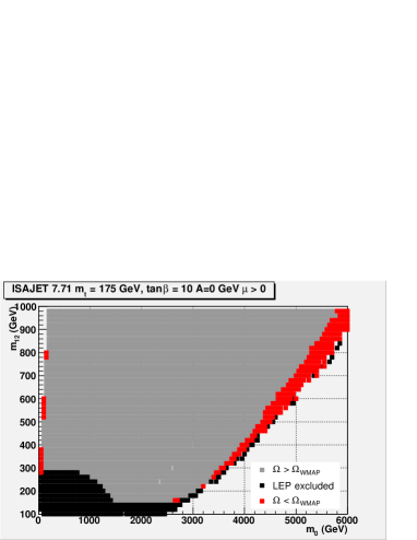
Figure 1: The picture shows the regions of the $(m_{0},m_{1/2})$ mSUGRA plane which have a neutralino relic density compatible with cosmological measurements in red/dark gray. The black region is excluded by LEP. The light gray region has a neutralino relic density which exceeds cosmological constraints. White regions are theoretically excluded. The values of $\tan\beta=10$, $A_{0}=0$, a positive $\mu$, and a top mass of 175 GeV were used.

In Fig. 1 a scan of the $(m_{0},m_{1/2})$ plane is presented, for fixed values of $\tan\beta=10$, $A_{0}=0$, and positive $\mu$. A top mass of 175 GeV was used. The red/dark gray region on the left is the stau coannihilation strip, while that on the right is the focus-point region with $\Omega_{\chi}<\Omega_{DM}$.

The latter is found at large value of $m_{0}>3$ TeV, hence the scalar particles are very heavy, near or beyond the sensitivity limit of LHC searches. Since $m_{1/2}<<m_{0}$, the gaugino (chargino and neutralino) and gluino states are much lighter. The SUSY production cross section at the LHC is thus dominated by gaugino and gluino pair production.

The dependence of the position of the focus-point region on mSUGRA and Standard Model parameters (in particular, the top mass) and the uncertainties related to the aproximations used by different RGE codes are discussed elsewhere [8, 9, 10].

Particle	Mass (GeV)	Particle	Mass (GeV)	Particle	Mass (GeV)
$\chi^{0}_{1}$	103.35	$\tilde{b}_{1}$	2924.8	$\tilde{\nu}_{\tau}$	3532.3
$\chi^{0}_{2}$	160.37	$\tilde{b}_{2}$	3500.6	$h$	119.01
$\chi^{0}_{3}$	179.76	$\tilde{t}_{1}$	2131.1	$H^{0}$	3529.7
$\chi^{0}_{4}$	294.90	$\tilde{t}_{2}$	2935.4	$A^{0}$	3506.6
$\chi^{\pm}_{1}$	149.42	$\tilde{e}_{L}$	3547.5	$H^{\pm}$	3530.6
$\chi^{\pm}_{2}$	286.81	$\tilde{e}_{R}$	3547.5
g̃	856.59	$\tilde{\nu}_{e}$	3546.3
$\tilde{u}_{L}$	3563.2	$\tilde{\tau}_{1}$	3519.6
$\tilde{u}_{R}$	3574.2	$\tilde{\tau}_{2}$	3533.7

Table 1: Mass of the supersymmetric particles for the benchmark point described in the text.

The following point in the parameter space was chosen for the detailed study reported in the next sections:

$$m_{0}=3550\mbox{GeV},m_{1/2}=300\mbox{GeV},A_{0}=0\mbox{GeV},\mu>0,\tan\beta=10$$

with the top mass set to 175 GeV and the mass spectrum computed with ISAJET. In table 1 the mass of SUSY particles for this point are reported. The scalar partners of Standard Model fermions have a mass larger than 2 TeV. The neutralinos and charginos have masses between 100 GeV and 300 GeV. The gluino is the lightest colored state, with a mass of 856.6 GeV. The lightest Higgs boson has a mass of 119 GeV, while the other Higgs states have a mass well beyond the LHC reach at more than 3 TeV.

The total SUSY production cross section at the LHC, as computed by HERWIG [11, 12, 13], is 5.00 pb. It is dominated by the production of gaugino pairs, $\chi^{0}\chi^{0}$ (0.22 pb), $\chi^{0}\chi^{\pm}$ (3.06 pb), and $\chi^{\pm}\chi^{\pm}$ (1.14 pb).

The production of gluino pairs (0.58 pb) is also significant. The gluino decays into $\chi^{0}qq$ (29.3%), $\chi^{0}g$ (6.4%), or $\chi^{\pm}qq^{{}^{\prime}}$ (54.3%). The quarks in the final state belongs to the third generation in 75.6% of the decays.

The direct production of gaugino pairs is difficult to separate from the Standard Model background; one possibility is to select events with several leptons, arising from the leptonic decays of neutralinos and charginos.

The production of gluino pairs can be separated from the Standard Model by requiring the presence of several high-$p_{T}$ jets and missing transverse energy. The presence of $b$-jets and leptons from the top and gaugino decays can also be used.

In the analysis presented here, the event selection is based on the multijet+missing energy signature. This strategy selects the events from gluino pair production, while rejecting both the Standard Model background and most of the gaugino direct production.

3 INCLUSIVE SEARCHES

The production of Supersymmetry events at the LHC was simulated using HERWIG 6.55 [11, 12, 13]. The top background was produced using MC@NLO 2.31 [14, 15]. The fully inclusive $t\bar{t}$ production was simulated. This is expected to be the dominant Standard Model background for the analysis presented in this note. The W+jets, and Z+jets background were produced using PYTHIA 6.222 [16, 17]. The vector bosons were forced to decay leptonically, and the transverse momentum of the W and the Z at generator level was required to be larger than 120 GeV and 100 GeV, respectively.

The events were then processed by ATLFAST [18] to simulate the detector response.

The most abundant gluino decay modes are $\tilde{g}\rightarrow\chi^{0}t\bar{t}$ and $\tilde{g}\rightarrow\chi^{\pm}tb$. Events with gluino pair production have thus at least four hard jets, and may have many more additional jets because of the top hadronic decay modes and the chargino and neutralino decays. When both gluinos decay to third generation quarks at least 4 jets are $b$-jets. A missing energy signature is provided by the two $\chi^{0}_{1}$ in the final state, and possibly by neutrinos coming from the top quark and the gaugino leptonic decay modes.

The following selections were made to separate these events from the Standard Model background:

• At least one jet with $p_{T}>120$ GeV

• At least four jets with $p_{T}>50$ GeV, and at least two of them tagged as $b$-jets.

• $E_{MISS}^{T}>100$ GeV

• $0.1<E_{MISS}^{T}/M_{EFF}<0.35$

• No isolated lepton (electron or muon) with $p_{T}>20$ GeV and $|\eta|<2.5$.

Here, the effective mass $M_{EFF}$ is defined as the scalar sum of the transverse missing energy and the transverse momentum of all the reconstructed hadronic jets.

Sample	Events	Basic cuts	2 $b$-jets
SUSY	50000	2515	1065
$t\bar{t}$	7600000	67089	11987
$W$+jets	3000000	16106	175
$Z$+jets	1900000	6991	147

Table 2: Efficiency of the cuts used for the inclusive search, evaluated with ATLFAST events for low luminosity operation. The number of events corresponds to an integrated luminosity of 10 $\mbox{fb}^{-1}$. The third column reports the number of events which passes the cuts described in the text, except the requirement of two b-jets, which is reported in the last column.

The efficiency of these cuts is reported in Tab. 2. The third column reports the number of events which passes the selections reported above, except the requirement of two $b$-jets, which is added to obtain the numbers in the last column. The standard ATLAS b-tagging efficiency of 60% for a rejection factor of 100 on light jets is assumed.

The SUSY events which pass the selection are almost exclusively due to gluino pair production; the gaugino direct production (about 90% of the total SUSY cross section) does not pass the cuts on jets and missing energy. After all selections the dominant background is by far due to $t\bar{t}$ production. The requirement of two $b$-jets supresses the remaining $W$+jets and $Z$+jets backgrounds by two orders of magnitude and is also expected to reduce the background from QCD multi-jet production (which has not been simulated) to negligible levels.

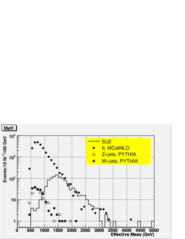
Figure 2: Distribution of the effective mass defined in the text, for SUSY events and the Standard Model backgrounds. The number of events correspond to an integrated luminosity of 10 $\mbox{fb}^{-1}$.

The distribution of the effective mass after these selection cuts is reported in Fig. 2. The statistic corresponds to an integrated luminosity of 10 $\mbox{fb}^{-1}$. The signal/background ratio for an effective mass larger than 1500 GeV is close to 1 and the statistical significance is $SUSY/\sqrt{SM}=23$.

4 THE DI-LEPTON EDGE

For the selected benchmark, the decays

$$\chi^{0}_{2}\rightarrow\chi^{0}_{1}l^{+}l^{-}$$ (1)

$$\chi^{0}_{3}\rightarrow\chi^{0}_{1}l^{+}l^{-}$$ (2)

occur with a branching ratio of 3.3% and 3.8% per lepton flavour respectively. The two leptons in the final state provide a natural trigger and a clear signature. Their invariant mass has a kinematic maximum equal to the mass difference of the two neutralinos involved in the decay, which is

$$m_{\chi^{0}_{2}}-m_{\chi^{0}_{1}}=57.02\;\mbox{GeV}\;\;m_{\chi^{0}_{3}}-m_{\chi^{0}_{1}}=76.41\;\mbox{GeV}$$ (3)

The analysis of the simulated data was performed with the following selections:

• Two isolated leptons with opposite charge and same flavour with $p_{T}>10$ GeV and $|\eta|<2.5$

• $E^{T}_{MISS}>80$ GeV, $M_{EFF}>1200$ GeV, $0.06<E^{T}_{MISS}/M_{EFF}<0.35$

• At least one jet with $p_{T}>80$ GeV, at least four jets with $p_{T}>60$ GeV and at least six jets with $p_{T}>40$ GeV

The efficiency of the various cuts is reported in table 3 for an integrated statistics of 10 $\mbox{fb}^{-1}$. After all cuts, 107 SUSY and 13 Standard Model events are left with a 2-lepton invariant mass smaller than 80 GeV. The dominant Standard Model background comes from $t\bar{t}$ production, and it is small compared to the SUSY combinatorial background: only half of the selected SUSY events do indeed have the decay (1) or (2) in the Montecarlo Truth record.

It should be noted that with these selections, the ratio $SUSY/\sqrt{SM}$ is 30, which is slightly larger than the significance provided by the selections of the inclusive search with lepton veto. The two lepton signature, with missing energy and hard jet selections is thus an excellent SUSY discovery channel.

Sample	Events	after cuts	$M_{ll}<80$ GeV
SUSY	50000	185	107
$t\bar{t}$	7600000	31	13
$W$+jets	3000000	0	0
$Z$+jets	1200000	1	0

Table 3: Efficiency of the cuts used for the reconstruction of the neutralino leptonic decay. The number of events corresponds to an integrated luminosity of 10 $\mbox{fb}^{-1}$. The third column contains the number of events which passes the selection cuts described in the text. The last column reports the number of the events passing the cuts which have an invariant mass of the two leptons lower than 80 GeV.

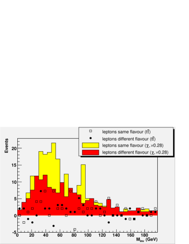
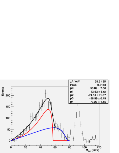
Figure 3: Left: Distribution of the invariant mass of lepton pairs with opposite charge and the same flavour (SUSY events: yellow histogram; Standard Model: open markers) or opposite flavour (SUSY events: red histogram; Standard Model: full markers). The number of events correspond to an integrated luminosity of 10 $\mbox{fb}^{-1}$. Right: Flavour-subtracted distribution of the invariant mass of lepton pairs, for an integrated luminosity of 300 $\mbox{fb}^{-1}$. The fit function is superimposed as a black line; the contribution it receives from the $\chi^{0}_{2}$ and $\chi^{0}_{3}$ decays are shown separately as a red and green line respectively. The fit parameters are the two normalizations (p0 and p1), the $\chi^{0}_{1}$ mass (p2), the $\chi^{0}_{2}-\chi^{0}_{1}$ mass difference (p3) and the $\chi^{0}_{3}-\chi^{0}_{1}$ mass difference (p4).

The combinatorial background can be estimated from the data using the $e^{+}\mu^{-}$ and $\mu^{+}e^{-}$ pairs. In the leftmost plot of Fig. 3 the distribution of the lepton invariant mass is reported for SUSY events with the same (different) flavour as yellow (red) histograms. Outside the signal region and the Z peak the two histograms are compatible. The Standard Model distribution is also reported for the same (different) flavour as open (closed) markers . Since the Standard Model background is small compared to the SUSY combinatorial background, it is neglected in the results reported below.

The flavour subtracted distribution is reported in the rightmost plot of Fig. 3 for an integrated luminosity of 300 $\mbox{fb}^{-1}$. The presence of two edges is apparent.

In order to fit the distribution, the matrix element and phase space factors given in Ref. [19] were used to compute an analytical expression for the invariant mass of the two leptons, under the aproximation that the Feynman diagram with slepton exchange is negligible compared to the Z exchange (this aproximation is justified for the Focus Point since sleptons are very heavy). The result is [10]

$$\frac{d\Gamma}{dm}=Cm\frac{\sqrt{m^{4}-m^{2}(\mu^{2}+M^{2})+(\mu M)^{2}}}{(m^{2}-m^{2}_{Z})^{2}}[-2m^{4}+m^{2}(2M^{2}+\mu^{2})+(\mu M)^{2}]$$ (4)

In the formula, $C$ is a normalization constant, $\mu=m_{2}-m_{1}$ and $M=m_{2}+m_{1}$, where $m_{1}$ and $m_{2}$ are the signed mass eigenvalues of the daughter and parent neutralino respectively. For the focuspoint, the mass eigenvalues of the two lightest neutralinos have the same sign, while the $\chi_{0}^{3}$ has the different sign.

The fit was performed with the sum of the $\chi^{0}_{3}$ and $\chi^{0}_{2}$ decay distributions provided by Eq. 4, convoluted with a gaussian smearing of 1.98 GeV. The smearing value was obtained from the width of the observed $Z$ peak. The fit parameters are the mass of the $\chi^{0}_{1}$ (which is the same for the two decays), the two mass differences $\chi^{0}_{2}-\chi^{0}_{1}$ and $\chi^{0}_{3}-\chi^{0}_{1}$, and the normalizations of the two decays.

The values found for the two mass differences are $m(\chi^{0}_{2})-m(\chi^{0}_{1})=(57.0\pm 0.5)$ GeV and $m(\chi^{0}_{3})-m(\chi^{0}_{1})=(77.3\pm 1.2)$ GeV. They are compatible with the true values (eq. 3).

The fit provides also the value of the mass of the $\chi^{0}_{1}$ since the shape of the distribution depends on it. This dependence is however very mild, expecially for $m(\chi^{0}_{1})>m(\chi^{0}_{i})-m(\chi^{0}_{1})$, and the limited statistics only allows to place a lower limit of about 20 GeV on the mass of the lightest neutralino.

5 CONCLUSIONS

A preliminary study of the ATLAS potential to study Supersymmetry in the Focus-Point scenario has been presented. This scenario is relatively difficult for the LHC, because of the large mass of the SUSY scalars (2-3 TeV).

For the selected point in the parameter space the observation of an excess of events with hard jets and missing energy over the Standard Model expectations should still be observed rather early. A statistical significance of more than 20 standard deviations is obtained for an integrated luminosity of $10\leavevmode\nobreak\ \mbox{fb}^{-1}$ both in the channel with no leptons and two $b$-tagged jets and the one with an opposite-sign electron or muon pair.

With a larger integrated luminosity of $300\;\mbox{fb}^{-1}$, corresponding to about three years at the design LHC luminosity, the two kinematical edges from the leptonic decay of the $\chi^{0}_{2}$ and the $\chi^{0}_{3}$ would be measured with a precision of the order of 1 GeV, providing two contraints on the masses of the three lightest neutralinos.

Acknowledgements

We thank members of the ATLAS collaboration for helpful discussions. We have made use of ATLAS physics analysis and simulation tools which are the result of collaboration-wide efforts.

Part 3 SUSY parameter determination in the challenging focus point-inspired case

K. Desch, J. Kalinowski, G. Moortgat-Pick and K. Rolbiecki

1 INTRODUCTION

Due to the unknown mechanism of SUSY breaking, supersymmetric extensions of the Standard Model contain a large number of new parameters: 105 in the Minimal Supersymmetric Standard Model (MSSM) appear and have to be specified. Experiments at future accelerators, the LHC and the ILC, will have not only to discover SUSY but also to determine precisely the underlying scenario without theoretical prejudices on the SUSY breaking mechanism. Particularly challenging are scenarios, where the scalar SUSY particle sector is heavy, as required e.g. in focus point scenarios (FP) as well as in split SUSY (sS). For a recent study of a mSUGRA FP scenario at the LHC, see [20].

Many methods have been worked out how to derive the SUSY parameters at collider experiments [21, 22]. In [23, 24, 25, 26, 27] the chargino and neutralino sectors have been exploited to determine the MSSM parameters. However, in most cases only the production processes have been studied and, furthermore, it has been assumed that the masses of scalar particles are already known. In [28] a fit has been applied to the chargino production in order to derive $M_{2}$, $\mu$, $\tan\beta$ and $m_{\tilde{\nu}_{e}}$. However, in the case of heavy scalars such fits lead to a rather weak constraint for $m_{\tilde{\nu}_{e}}$.

Since it is not easy to determine experimentally cross sections for production processes, studies have been made to exploit the whole production-and-decay process. Angular and energy distributions of the decay products in production with subsequent three-body decays have been studied for chargino as well as neutralino processes in [29, 30, 31]. Since such observables depend strongly on the polarization of the decaying particle the complete spin correlations between production and decay can have large influence and have to be taken into account: Fig. 1 shows the effect of spin correlation on the forward-backward asymmetry as a function of sneutrino mass in the scenario considered below. Exploiting such spin effects, it has been shown in [32, 33] that, once the chargino parameters are known, useful indirect bounds for the mass of the heavy virtual particles could be derived from forward-backward asymmetries of the final lepton $A_{FB}(\ell)$.

2 CHOSEN SCENARIO: FOCUS POINT-INSPIRED CASE

In this section we take a FP-inspired mSUGRA scenario defined at the GUT scale [34]. However, in order to assess the possibility of unravelling such a challenging new physics scenario our analysis is performed entirely at the EW scale without any reference to the underlying SUSY breaking mechanism. The parameters at the EW scale are obtained with the help of SPheno code [35]; with the micrOMEGA code [6] it has been checked that the lightest neutralino provides the relic density consistent with the non-baryonic dark matter. The low-scale gaugino/higgsino/gluino masses as well as the derived masses of SUSY particles are listed in Tables 1, 2. As can be seen, the chargino/neutralino sector as well as the gluino are rather light, whereas the scalar particles are about 2 TeV (with the only exception of $h$ which is a SM-like light Higgs boson).

$M_{1}$	$M_{2}$	$M_{3}$	$\mu$	$\tan\beta$	$m_{\tilde{\chi}^{\pm}_{1}}$	$m_{\tilde{\chi}^{\pm}_{2}}$	$m_{\tilde{\chi}^{0}_{1}}$	$m_{\tilde{\chi}^{0}_{2}}$	$m_{\tilde{\chi}^{0}_{3}}$	$m_{\tilde{\chi}^{0}_{4}}$	$m_{\tilde{g}}$
60	121	322	540	20	117	552	59	117	545	550	416

Table 1: Low-scale gaugino/higgsino/$\tan\beta$ MSSM parameters and the resulting chargino and neutralino masses. All masses are given in [GeV].

$m_{h}$	$m_{H,A}$	$m_{H^{\pm}}$	$m_{\tilde{\nu}}$	$m_{\tilde{\ell}_{R}}$	$m_{\tilde{e}_{L}}$	$m_{\tilde{\tau}_{1}}$	$m_{\tilde{\tau}_{2}}$	$m_{\tilde{q}_{R}}$	$m_{\tilde{q}_{L}}$	$m_{\tilde{t}_{1}}$	$m_{\tilde{t}_{2}}$
119	1934	1935	1994	1996	1998	1930	1963	2002	2008	1093	1584

Table 2: Masses of the SUSY Higgs particles and scalar particles, all masses are given in [GeV].

Figure 1: Forward-backward asymmetry of $e^{-}$ in the process $e^{+}e^{-}\to\tilde{\chi}^{+}_{1}\tilde{\chi}^{-}_{1}$, $\tilde{\chi}^{-}_{1}\to\tilde{\chi}^{0}_{1}e^{-}\bar{\nu}_{e}$ as a function of $m_{\tilde{\nu}_{e}}$ in a) the range $m_{\tilde{\nu}_{e}}=[200,2300]$ GeV (left) and in b) $m_{\tilde{\nu}_{e}}=[1750,2250]$ GeV (right), both at $\sqrt{s}=350$ GeV and for unpolarized beams. The mass of the other scalar virtual particle, $m_{\tilde{e}_{L}}$, which contributes in the decay process, has been assumed to fulfil the SU(2) mass relation $m^{2}_{\tilde{e}_{L}}=m_{\tilde{\nu}_{e}}^{2}+m_{Z}^{2}\cos(2\beta)(-1+\sin^{2}\theta_{W})$. In a) the light (green) line denotes the derived $A_{FB}(e^{-})$ without taking into account the chargino spin correlations between production and decay process.

2.1 EXPECTATIONS AT THE LHC

As can be seen from Tables 1, 2, all squark particles are kinematically accessible at the LHC. The largest squark production cross section is for $\tilde{t}_{1,2}$. However, with stops decaying mainly to $\tilde{g}t$ [with $BR(\tilde{t}_{1,2}\to\tilde{g}t)\sim 66\%$], where background from top production will be large, no new interesting channels are open in their decays. The other squarks decay mainly via $gq$, but since the squark masses are very heavy, $m_{\tilde{q}_{L,R}}>2$ TeV, mass reconstruction will be difficult. Nevertheless, the indication that the scalar fermions are very heavy will be very important in narrowing theoretical uncertainty on the chargino and neutralino decay branching ratios.

In this scenario the inclusive discovery of SUSY at the LHC is possible mainly to the large gluino production cross section. The gluino production is expected with very high rates. Therefore several gluino decay channels can be exploited. The largest branching ratio for the gluino decay in our scenario is into neutralinos $BR(\tilde{g}\to\tilde{\chi}^{0}_{2}b\bar{b})\sim 14\%$ with a subsequent leptonic neutralino decay $BR(\tilde{\chi}^{0}_{2}\to\tilde{\chi}^{0}_{1}\ell^{+}\ell^{-})$, $\ell=e,\mu$ of about 6%, see Table 3. In this channel the dilepton edge will clearly be visible since this process is practically background-free. The mass difference between the two light neutralino masses could be measured from the dilepton edge with an uncertainty of about [34]

$$\delta(m_{\tilde{\chi}^{0}_{2}}-m_{\tilde{\chi}^{0}_{1}})\sim 0.5\leavevmode\nobreak\ \mathrm{GeV}.$$ (1)

Other frequent gluino decays are into the light chargino and jets, with about $BR(\tilde{g}\to\tilde{\chi}^{\pm}_{1}qq^{\prime})\sim 20\%$ for $qq^{\prime}$ in the first two families, and about $3\%$ in the third.

$BR(\tilde{g}\to\tilde{\chi}^{0}_{2}b\bar{b})$	$14.4\%$	$BR(\tilde{g}\to\tilde{\chi}^{-}_{1}q_{u}\bar{q}_{d})$	$10.8\%$	$BR(\tilde{\chi}^{+}_{1}\to\tilde{\chi}^{0}_{1}\bar{q}_{d}q_{u})$	$33.5\%$
$BR(\tilde{\chi}^{0}_{2}\to\tilde{\chi}^{0}_{1}\ell^{+}\ell^{-})$	$3.0\%$	$BR(\tilde{t}_{1,2}\to\tilde{g}t)$	$66\%$	$BR(\tilde{\chi}^{-}_{1}\to\tilde{\chi}^{0}_{1}\ell^{-}\nu_{\ell})$	$11.0\%$

Table 3: Branching ratios for some important decay modes in our scenario, $\ell=e,\mu,\tau$, $q_{u}=u,c$, $q_{d}=d,s$. Numbers are given for each family separately.

2.2 EXPECTATIONS AT THE ILC

At the ILC with $\sqrt{s}=500$ GeV only light charginos and neutralinos are kinematically accessible. However, in this scenario the neutralino sector is characterized by very low production cross sections, below 1 fb, so that it might not be fully exploitable. Only the chargino pair production process has high rates at the ILC and all information obtainable from this sector has to be used. In the following we study the process

$$e^{+}e^{-}\to\tilde{\chi}^{+}_{1}\tilde{\chi}^{-}_{1}$$ (2)

with subsequent chargino decays

$$\tilde{\chi}^{-}_{1}\to\tilde{\chi}^{0}_{1}e^{-}\bar{\nu}_{e},\quad{\rm and}\quad\tilde{\chi}^{-}_{1}\to\tilde{\chi}^{0}_{1}s\bar{c}$$ (3)

for which the analytical formulae including the complete spin correlations are given in a compact form e. g. in [29]. The production process occurs via $\gamma$ and $Z$ exchange in the $s$-channel and $\tilde{\nu}_{e}$ exchange in the $t$-channel, and the decay processes get contributions from $W^{\pm}$-exchange and $\tilde{\nu}_{e}$, $\tilde{e}_{L}$ (leptonic decays) or $\tilde{s}_{L}$, $\tilde{c}_{L}$ (hadronic decays).

Table 4 lists the chargino production cross sections and forward-backward asymmetries for different beam polarization configurations and the $1\sigma$ statistical uncertainty based on ${\cal L}=200$ fb^-1 for each polarization configuration, $(P_{e^{-}},P_{e^{+}})=(-90\%,+60\%)$ and $(+90\%,-60\%)$. Below we constrain our analyses to the first step of the ILC with $\sqrt{s}\leq 500$ GeV and study only the $\tilde{\chi}^{+}_{1}\tilde{\chi}^{-}_{1}$ production and decay.

Studies of chargino production with semi-leptonic decays at the ILC runs at $\sqrt{s}=350$ and $500$ GeV will allow to measure the light chargino mass in the continuum with an error $\sim 0.5$ GeV. This can serve to optimize the ILC scan at the threshold [36] which, due to the steep $s$-wave excitation curve in $\tilde{\chi}^{+}_{1}\tilde{\chi}^{-}_{1}$ production, can be used to determine the light chargino mass very precisely to about [37, 38, 39]

$$m_{\tilde{\chi}^{\pm}_{1}}=117.1\pm 0.1\leavevmode\nobreak\ \mathrm{GeV}.$$ (4)

The light chargino has a leptonic branching ratio of about $BR(\tilde{\chi}^{-}_{1}\to\tilde{\chi}^{0}_{1}\ell^{-}\bar{\nu}_{\ell})\sim 11\%$ for each family and a hadronic branching ratio of about $BR(\tilde{\chi}^{-}_{1}\to\tilde{\chi}^{0}_{1}s\bar{c})\sim 33\%$. The mass of the lightest neutralino $m_{\tilde{\chi}^{0}_{1}}$ can be derived either from the energy distribution of the lepton $\ell^{-}$ or in hadronic decays from the invariant mass distribution of the two jets. We therefore assume [34]

$$m_{\tilde{\chi}^{0}_{1}}=59.2\pm 0.2\leavevmode\nobreak\ \mathrm{GeV}.$$ (5)

Together with the information from the LHC, Eq. (1), a mass uncertainty for the second lightest neutralino of about

$$m_{\tilde{\chi}^{0}_{2}}=117.1\pm 0.5\leavevmode\nobreak\ \mathrm{GeV}.$$ (6)

can be assumed.

3 PARAMETER DETERMINATION

3.1 Parameter fit without using the forward-backward asymmetry

In the fit we use polarized chargino cross section multiplied by the branching ratios of semi-leptonic chargino decays: $\sigma(e^{+}e^{-}\to\tilde{\chi}^{+}_{1}\tilde{\chi}^{-}_{1})\times BR$, with $BR=2\times BR(\tilde{\chi}^{+}_{1}\to\tilde{\chi}^{0}_{1}\bar{q}_{d}q_{u})\times BR(\tilde{\chi}^{-}_{1}\to\tilde{\chi}^{0}_{1}\ell^{-}\bar{\nu})+[BR(\tilde{\chi}^{-}_{1}\to\tilde{\chi}^{0}_{1}\ell^{-}\bar{\nu})]^{2}\sim 0.34$, $\ell=e,\mu$, $q_{u}=u,c$, $q_{d}=d,s$, as given in Table 4. We take into account $1\sigma$ statistical error, a relative uncertainty in polarization of $\Delta P_{e^{\pm}}/P_{e^{\pm}}=0.5\%$ [40] and an experimental efficiency of 50%, cf. Table 4.

We applied a four-parameter fit for the parameters $M_{1}$, $M_{2}$, $\mu$ and $m_{\tilde{\nu}_{e}}$ for fixed $\tan\beta=5$,10,15,20,25,30 values. Fixing $\tan\beta$ was necessary for a proper convergence of the minimalization procedure. For the input value $\tan\beta=20$ we obtain

$$M_{1}=60.0\pm 0.2\leavevmode\nobreak\ \mathrm{GeV},\quad M_{2}=121.0\pm 0.7\leavevmode\nobreak\ \mathrm{GeV},\quad\mu=540\pm 50\leavevmode\nobreak\ \mathrm{GeV},\quad m_{\tilde{\nu}_{e}}=2000\pm 100\leavevmode\nobreak\ \mathrm{GeV}.$$ (7)

Due to the strong gaugino component of $\tilde{\chi}^{\pm}_{1}$ and $\tilde{\chi}^{0}_{1,2}$, the parameters $M_{1}$ and $M_{2}$ are well determined with a relative uncertainty of $\sim 0.5\%$. The higgsino parameter $\mu$ as well as $m_{\tilde{\nu}_{e}}$ are determined to a lesser degree, with relative errors of $\sim 10\%$ and 5%. Note however, that the errors, as well as the fitted central values depend on $\tan\beta$. Figure 2 shows the migration of 1$\sigma$ contours in $m_{\tilde{\nu}_{e}}$–$M_{2}$ (left), $M_{2}$–$\mu$ (middle) and $M_{1}$–$M_{2}$ (right) panels.

Figure 2: Migration of 1$\sigma$ contours with $\tan\beta=5,\,10,\,20,\,30$ (top-to-bottom in the left panel, right-to-left in the middle panel, top-to-bottom in the right panel).

Varying $\tan\beta$ between 5 and 30 leads to a shift $\sim 1$ GeV of the fitted $M_{1}$ value and $\sim 3.5$ GeV of $M_{2}$, increasing effectively their experimental errors, while the migration effect for $\mu$ and $m_{\tilde{\nu}_{e}}$ is much weaker.

3.2 Parameter fit including the forward-backward asymmetry

Following the method proposed in [32, 33] we now extend the fit by using as additional observable the forward-backward asymmetry of the final electron. As explained in the sections before, this observable is very sensitive to the mass of the exchanged scalar particles, even for rather heavy masses, see Fig. 1 (right). Since in the decay process also the left selectron exchange contributes the $SU(2)$ relation between the left selectron and sneutrino masses: $m^{2}_{\tilde{e}_{L}}=m_{\tilde{\nu}_{e}}^{2}+m_{Z}^{2}\cos(2\beta)(-1+\sin^{2}\theta_{W})$ has been assumed [21]. In principle this assumption could be tested by combing the leptonic forward-backward asymmetry with that in the hadronic decay channels if the squark masses could be measured at the LHC [34].

$\sqrt{s}$/GeV	$(P_{e^{-}},P_{e^{+}})$	$\sigma(\tilde{\chi}^{+}_{1}\tilde{\chi}^{-}_{1})$/fb	$\sigma(\tilde{\chi}^{+}_{1}\tilde{\chi}^{-}_{1})\times BR$/fb	$A_{FB}(e^{-})$/%
350	$(-90\%,+60\%)$	6195.5$\pm$7.9	2127.9$\pm$4.0	4.49$\pm$0.32
	$(0,0)$	2039.1$\pm$4.5	700.3$\pm$2.7	4.5$\pm 0.5$
	$(+90\%,-60\%)$	85.0$\pm$0.9	29.2$\pm 0.7$	4.7$\pm 2.7$
500	$(-90\%,+60\%)$	3041.5$\pm$5.5	1044.6$\pm 2.3$	4.69$\pm$0.45
	$(0,0)$	1000.6$\pm$3.2	343.7$\pm 1.7$	4.7$\pm 0.8$
	$(+90\%,-60\%)$	40.3$\pm$0.4	13.8$\pm 0.4$	5.0$\pm 3.9$

Table 4: Cross sections for the process $e^{+}e^{-}\to\tilde{\chi}^{+}_{1}\tilde{\chi}^{-}_{1}$ and forward-backward asymmetries for this process followed by $\tilde{\chi}^{-}_{1}\to\tilde{\chi}^{0}_{1}e^{-}\nu_{e}$, for different beam polarization $P_{e^{-}}$, $P_{e^{+}}$ configurations at the cm energies $\sqrt{s}=350$ GeV and $500$ GeV at the ILC. Errors include $1\sigma$ statistical uncertainty assuming ${\cal L}=200$ fb^-1 for each polarization configuration, and beam polarization uncertainty of 0.5%. $BR\simeq 0.34$, cf. Sec. 3.1 and Table 3.

We take into account a $1\sigma$ statistical uncertainty for the asymmetry which is given by

$$\Delta(A_{FB})=2\sqrt{\epsilon(1-\epsilon)/N},$$ (8)

where $\epsilon=\sigma_{F}/(\sigma_{F}+\sigma_{B})$ and the number of events is denoted by $N$. Due to high production rates, the uncertainty is rather small, see Table 4.

Applying now the 4-parameter fit-procedure and combining it with the forward-backward asymmetry leads to:

$$M_{1}=60.0\pm 0.4\leavevmode\nobreak\ \mathrm{GeV},\quad M_{2}=121.0\pm 1.5\leavevmode\nobreak\ \mathrm{GeV},\quad\mu=540\pm 50\leavevmode\nobreak\ \mathrm{GeV}$$

$$m_{\tilde{\nu}_{e}}=1995\pm 60\leavevmode\nobreak\ \mathrm{GeV},\quad\tan\beta>10.$$ (9)

Including the leptonic forward-backward asymmetry in the multi-parameter fit strongly improves the constraints for the heavy virtual particle, $m_{\tilde{\nu}_{e}}$. Furthermore no assumptions on $\tan\beta$ has to be made. Since for small $\tan\beta$ the wrong value of $A_{FB}$ is predicted, $\tan\beta$ is constrained from below. The constraints for the mass $m_{\tilde{\nu}_{e}}$ are improved by about a factor 2 and for gaugino mass parameters $M_{1}$ and $M_{2}$ by a factor 3, as compared to the results of the previous section with unconstrained $\tan\beta$. The error for the higgsino mass parameter $\mu$ remains roughly the same. It is clear that in order to improve considerably the constraints for the parameter $\mu$ the measurement of the heavy higgsino-like chargino and/or neutralino masses will be necessary at the second phase of the ILC with $\sqrt{s}\sim 1000$ GeV.

4 CONCLUSIONS

In [34] we show the method for constraining heavy virtual particles and for determining the SUSY parameters in focus-point inspired scenarios. Such scenarios appear very challenging since there is only a little experimental information about the SUSY sector accessible. However, we show that a careful exploitation of data leads to significant constraints for unknown parameters. The most powerful tool in this kind of analysis turns out to be the forward-backward asymmetry. The proper treatment of spin correlations between the production and the decay is a must in that context. This asymmetry is strongly dependent on the mass of the exchanged heavy particle. The $SU(2)$ assumption on the left selectron and sneutrino masses could be tested by combing the leptonic forward-backward asymmetry with the forward-backward asymmetry in the hadronic decay channels if the squark masses could be measured at the LHC [34]. We want to stress the important role of the LHC/ILC interplay since none of these colliders alone can provide us with data needed to perform the SUSY parameter determination in focus-like scenarios.

Acknowledgements

The authors would like to thank the organizers of Les Houches 2005 for the kind invitation and the pleasant atmosphere at the workshop. This work is supported by the European Community’s Human Potential Programme under contract HPRN-CT-2000-00149 and by the Polish State Committee for Scientific Research Grant No 2 P03B 040 24.

Part 4 mSUGRA validity of the Barr neutralino spin analysis at the LHC

B.C. Allanach and F. Mahmoudi

If signals consistent with supersymmetry (SUSY) are discovered at the LHC, it will be desirable to check the spins of SUSY particles in order to test the SUSY hypothesis directly. There is the possibility, for instance, of producing a similar spectrum of particles as the minimal supersymmetric standard model (MSSM) in the universal extra dimensions (UED) model [41]. In UED, the first Kaluza-Klein modes of Standard Model particles have similar couplings to their MSSM analogues, but their spins differ by $1/2$.

In a recent publication [42], Barr proposed a method to determine the spin of supersymmetric particles at the LHC from studying the $\tilde{q}\rightarrow{\chi}_{2}^{0}\,q\rightarrow\tilde{l}_{R}\,l_{n}\,q\rightarrow\chi_{1}^{0}l_{n}l_{f}\,q$ decay chain. Depending upon the charges of the various sparticles involved, the near and far leptons ($l_{n},l_{f}$ respectively) may have different charges. Forming the invariant mass of $l_{n}$ with the quark normalised to its maximum value: $\hat{m}\equiv m_{l_{n}q}/m_{l_{n}q}^{max}=\sin(\theta^{*}/2)$, where $\theta^{*}$ is the angle between the quark and near lepton in the $\chi_{2}^{0}$ rest frame. Barr’s central observation is that the probability distribution function $P_{1}$ for $l_{n}^{+}q$ or $l_{n}^{-}\bar{q}$ is different to $P_{2}$ (the probability distribution function of $l_{n}^{-}\bar{q}$ or $l_{n}^{+}\bar{q}$) due to different helicity factors:

$$\frac{dP_{1}}{d\hat{m}}=4{\hat{m}}^{3},\qquad\frac{dP_{2}}{d\hat{m}}=4\hat{m}(1-{\hat{m}}^{2}).$$ (1)

One cannot in practice distinguish $q$ (originating from a squark) from $\bar{q}$ (originating from an anti-squark), but instead averages the $q,\bar{q}$ distributions by simply measuring a jet. This sum may therefore be distinguished against the pure phase-space distribution

$$\frac{dP_{PS}}{d\hat{m}}=2\hat{m}$$ (2)

only if the expected number of produced squarks is different to the number of anti-squarks. Indeed, the distinguishing power of the spin measurement is proportional to the squark-anti squark production asymmetry. The relevant production processes are $pp\rightarrow{\tilde{q}}{\tilde{\bar{q}}}$, $\tilde{g}{\tilde{q}}$ or $\tilde{g}{\tilde{\bar{q}}}$. The latter two processes may have different cross-sections because of the presence of valence quarks in the proton parton distribution functions, which will favour squarks over anti-squarks. Such arguments can be extended to examine whether supersymmetry can be distinguished against UED at the LHC [43, 44].

Due to CPU time constraints, the spin studies in refs. [42, 43] were performed for a single point in mSUGRA parameter space (and a point in UED space in refs. [43, 44]). The points studied had rather light spectra, leading one to wonder how generic the possibility of spin measurements might be. Here, we perform a rough and simple estimate of the statistical significance of the squark/anti-squark asymmetry, in order to see where in parameter space the spin discrimination technique might work.

Provided that the number of (anti-)squarks produced is greater than about 10, we may use Gaussian statistics to estimate the significance of any squark/anti-squark asymmetry. Denoting $Q$ as the number of squarks produced and $\bar{Q}$ as the number of anti-squarks, the significance of the production asymmetry is

$$S=\frac{Q-\bar{Q}}{\sqrt{Q+\bar{Q}}}.$$ (3)

Eq. 3 does not take into account the acceptance $a$ of the detector or the branching ratio $b$ of the decay chain. Assuming squarks to lead to the same acceptances and branching ratios as anti-squarks, we see from Eq. 3 that the significance of the measured asymmetry is

$${\mathcal{S}}=\sqrt{ab}S.$$ (4)

The SUSY mass spectrum and decay branching ratios were calculated with ISAJET-7.72 [7]. We consider a region which contains the SPS 1a slope [45] $(m_{0}=0.4\times m_{1/2})$ and we choose the following mSUGRA parameters in order to perform a $m_{0}-m_{1/2}$ scan:

$$(A_{0}=-m_{0},\tan\beta=10,\mu>0)\;\;.$$ (5)

A sample of inclusive SUSY events was generated using PYTHIA-6.325 Monte Carlo event generator [46] assuming an integrated luminosity of 300 fb^-1 and the leading-order parton distribution functions of CTEQ 5L [47]. The LEP2 bound upon the lightest CP-even Higgs mass implies $m_{h^{0}}>114$ GeV for $\sin^{2}(\beta-\alpha)\approx 1$. For any given point in parameter space, we impose $m_{h^{0}}>111$ GeV on the ISAJET prediction of $m_{h^{0}}$, which allows for a 3 GeV error. We also impose simple-minded constraints from negative sparticle searches presented in Table 1.

Particle	$\chi^{0}_{1}$	$\tilde{l}_{R}$	$\tilde{\nu}_{e,\mu}$	$\chi^{\pm}_{1}$	$\tilde{t}_{1}$	$\tilde{g}$	$\tilde{b}_{1}$	$\tilde{\tau}_{1}$	$\tilde{q}_{R}$
Lower bound	37	88	43.1	67.7	86.4	195	91	76	250

Table 1: Lower bounds on sparticle masses in GeV, obtained from Ref. [48].

Figure 1: Significance in the ($m_{0}$-$m_{1/2}$) plane for 300 fb^-1 of integrated luminosity at the LHC for (a) the production asymmetry $S$ and (b) the measured asymmetry $S\sqrt{b}$ for the chain $\tilde{q}\rightarrow{\chi}_{2}^{0}\,q\rightarrow\tilde{l}_{R}\,l_{n}\,q\rightarrow\chi_{1}^{0}l_{n}l_{f}\,q$, assuming that the acceptance is equal to 1. The SPS 1a line is labelled in black with the SPS1a point marked as an asterisk. The red line delimits a charged lightest-supersymmetric particle (LSP) from an uncharged LSP. Contours of equal squark or gluino mass are shown in grey for reference. The magenta line delimits the region that does not pass sparticle or higgs search constraints (“excluded”) from the region that does. The significance is measured with respect to the bar on the right hand side of each plot, which is on a logarithmic scale. White regions correspond either to excluded points, or negligible significance.

Fig. 1 displays the production and measured asymmetries in the $m_{0}-m_{1/2}$ plane. In Fig. 1a, neither the acceptance of the detector nor the branching ratios of decays are taken into account. Thus, if the reader wishes to use some particular chain in order to measure a charge asymmetry, the significance plotted should be multiplied by $\sqrt{ba}$. As $m_{0}$ and $m_{1/2}$ grow, the relevant sparticles (squarks and gluinos) become heavier and the overall number of produced squarks decreases, leading to less significance. We see that much of the allowed part of the plane corresponds to a production asymmetry significance of greater than 10. However, the acceptance and branching ratio effects are likely to drastically reduce this number.

Fig. 1b includes the effect of the branching ratio for the chain that Barr studied in the significance. The significance is drastically reduced from Fig. 1a due to the small branching ratios involved. The region marked “charged LSP” is cosmologically disfavoured if the LSP is stable, but might be viable if R-parity is violated. In this latter case though, a different spin analysis would have to be performed due to the presence of the LSP decay products. The region marked “forbidden” occurs when $m_{{\tilde{l}}_{R}}>m_{\chi_{2}^{0}}$, implying that the decay chain studied by Barr does not occur.

The highest squark/anti-squark asymmetry can be found around $m_{0}=100$, $m_{1/2}=200$ and its significance is around 500 or so, including branching ratios. Barr investigated the mSUGRA point $m_{0}=100$ GeV , $m_{1/2}=300$ GeV, $A_{0}=m_{1/2}$, $\tan\beta=$ 2.1, $\mu>0$, assuming a luminosity of 500 fb^-1. In his paper, which includes acceptance effects, Barr states that a significant spin measurement at this point should still be possible even with only 150 fb^-1 of integrated luminosity. Our calculation of the significance $S\sqrt{b}$ for this point is 53. Assuming that the acceptance is not dependent upon the mSUGRA parameters, we may deduce that a value of $S\sqrt{b}>53$ in Fig. 1b is also viable with 150 fb^-1. This roughly corresponds to the orange and red regions in Fig. 1b. Although the parameter space is highly constrained, there is nevertheless a non-negligible region where the Barr spin analysis may work.

Acknowledgements

FM would like to thank Steve Muanza for his help regarding Pythia, and acknowledges the support of the McCain Fellowship at Mount Allison University. BCA thanks the Cambrige SUSY working group for suggestions. This work has been partially supported by PPARC.

Part 5 The trilepton signal in the focus point region

Ph. Gris, R. Lafaye, T. Plehn, L. Serin, L. Tompkins and D. Zerwas

1 INTRODUCTION

Recent high energy gamma ray observations from EGRET show an excess of galactic gamma rays in the 1 GeV range [49]. A possible explanation of the excess are photons generated by neutralino annihilation in galactic dark matter [50]. Unfortunately, this kind cosmological data is only sensitive to a few supersymmetric parameters, like the mass and the annihilation or detection cross sections of the weakly interacting dark matter candidate. A prime dark matter candidate is the lightest supersymmetric particle, which in most supersymmetry breaking scenarios turns out to be the lightest neutralino [51]. To be able to derive stronger statements from the data, one can assume gravity mediated supersymmetry breaking (mSUGRA) and fit the free parameters of this constrained model to the observed gamma ray spectrum [50]. Only an additional connection of this kind (assuming we know the supersymmetry breaking scenario) allows one to make statements about the scalar sector. In this brief letter, we study the mSUGRA parameter point given by $m_{0}=1400$ GeV, $m_{1/2}=180$ GeV, $A_{0}=700$ GeV, $\tan\beta=51$ and $\mu>0$, which could explain the claimed excess. We analyse the phenomenological implications for searches and measurements of supersymmetric particles at the Tevatron and at the LHC [52]. To determine the underlying mSUGRA parameters sophisticated tools such as Fittino [53, 54] and SFITTER [55, 56] are required. In our study we use SFITTER to determine the expected errors on the supersymmetric parameters.

The TeV-scale particle masses for our mSUGRA parameter point are displayed in Table 1. The high $m_{0}$   value [57, 58, 59] places most squarks and sleptons well above 1 TeV, which means that the expected production rate at the LHC will be strongly reduced as compared to the standard scenarios such as SPS1a [45]. The large value for $\tan\beta$   enhances the heavy Higgs Yukawa coupling to $b$ quarks and $\tau$ leptons. Therefore the MSSM Higgs sector is likely to be observed at the LHC, for example through a charged Higgs boson decaying to $\tau$ leptons [60, 61] or through a precision mass measurement for the heavy neutral Higgs bosons decaying to muon pairs [52]. Certainly, the comparably low-mass charginos, neutralinos and gluinos, will be produced at accelerator experiments.

Particle	Mass (GeV)	Particle	Mass (GeV)	Particle	Mass (GeV)
$\tilde{q}$	1430	$\tilde{g}$	520	$h^{0}$	114
$\tilde{b}$	974	$\tilde{\chi}_{1}^{\pm}$	137	$A^{0}$	488
$\tilde{l}$	1400	$\tilde{\chi}_{1}^{0}$	72
$\tilde{\tau}$	974	$\tilde{\chi}_{2}^{0}$	137

Table 1: TeV-scale supersymmetric particle masses in the EGRET parameter point computed with SUSPECT [62].

2 DISCOVERY PROSPECTS

At the Run II of the Tevatron, the 500 GeV gluinos are unlikely to be observed, in particular in the limit of heavy squarks, because the powerful squark–gluino associated production channel does not contribute to the gluino rate. Only the light gauginos $\tilde{\chi}_{1}^{\pm}$ , $\tilde{\chi}_{1}^{0}$ , $\tilde{\chi}_{2}^{0}$ might be observable. One of the most promising channels for SUSY discovery at the Tevatron is the production of a neutralino and a chargino with a subsequent decay to tri-leptons [63, 64, 65, 66, 67]: $p\bar{p}\rightarrow\tilde{\chi}_{1}^{\pm}\tilde{\chi}_{2}^{0}\rightarrow 3\ell+E_{T}+X$. Unfortunately, for our SUSY parameter point, its rate strongly auppressed by the heavy sleptons: the leading order cross section is only $\sigma\times BR\simeq 10$ fb, with mild next-to-leading order corrections [68]. Depending on the luminosity delivered by the Tevatron [69], between 40 and 80 events are expected per experiment running until 2009. Since the 67 GeV mass difference between the $\tilde{\chi}_{1}^{0}$ and the $\tilde{\chi}_{2}^{0}$ and $\tilde{\chi}_{1}^{\pm}$ is sizeable, the transverse momentum of the decay leptons is large. At the generator level, the $p_{T}$ distribution of the leading (next-to-leading) lepton peaks around 35 GeV (25 GeV). Hence, given a large enough ratem triggering on this signal will not be a problem. However, the cross-section is too low to allow a discovery: in Figure 1 [67] we see that an integrated luminosity of at least $20\leavevmode\nobreak\ fb^{-1}$ is required to claim a 5$\sigma$ discovery.

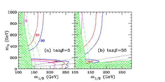
Figure 1: Tevatron reach in the trilepton channel in the $m_{0}-m_{1/2}$ plane, for fixed values of $A_{0}$, $\mu>0$ and $\tan\beta=5,35$. We show results for 2, 10 and 30 $fb^{-1}$ total integrated luminosity. The figure is taken out of Ref. [67]

At the LHC, the total inclusive SUSY particles production cross section for our parameter point is 19.8 pb. The largest contributions come from the processes $gg\rightarrow\tilde{g}\tilde{g}$ (50%), $q\bar{q}^{\prime}\rightarrow\tilde{\chi}_{2}^{0}\tilde{\chi}_{1}^{\pm}$ (20%), and $q\bar{q}\rightarrow\tilde{\chi}_{1}^{\pm}\tilde{\chi}_{1}^{\mp}$ (10%). The dominant source of SUSY particle production with a decay to hard jets are of course gluino decays. We can extract the tri-lepton signal [70, 71, 72, 73] $q\bar{q}\rightarrow\tilde{\chi}_{2}^{0}\tilde{\chi}_{1}^{\pm}\rightarrow\ell\ell\tilde{\chi}_{1}^{0},\ell\nu_{\ell}\tilde{\chi}_{1}^{0}$ by requiring exactly three leptons with a transverse momentum greater than 20 (10) GeV for electrons (muons).

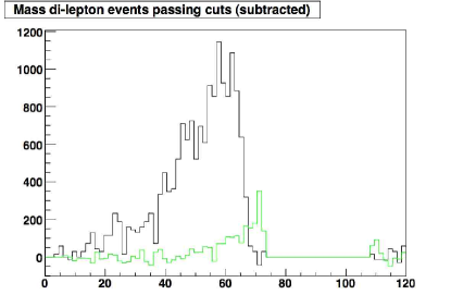
Figure 2: Invariant mass of dilepton pairs after cuts. We include 100 fb^-1 integrated luminosity at the LHC. Chargino-neutralino signal events are shown in black, the $WZ$ background in green. Opposite-sign opposite-flavor events are subtracted.

Process	Cut
	Lepton Production	3 lep	Z mass
$\tilde{\chi}_{2}^{0}+\tilde{\chi}_{1}^{\pm}$	129 fb	28 fb	13 fb
$WZ$	875 fb	144 fb	4.9 fb
$ZZ$	161 fb	21.9 fb	.0146 fb

Table 2: Cross sections for signal and background at the LHC. We show $\sigma\cdot\mathrm{BR}_{\ell\ell\ell}$ including taus (first column), the rate after requiring 3 identified leptons (second column), and events after the $m_{Z}$ mass window cut (third column).

The main backgrounds are $WZ$ and $ZZ$ production where one lepton is not reconstructed in the $ZZ$ case. To reject $ZZ$ events, we require the invariant mass of all opposite-sign, same-flavor lepton pairs to be outside a $5\sigma$ window around $m_{Z}$. The background events with a $W$ or with a $Z$ decaying to a leptonic $\tau$ are not affected by these cuts. The combinatorial background we remove through background subtraction (opposite-flavour opposite-sign leptons). The invariant mass distribution for dilepton pairs is shown in Figure 2. We list the corresponding cross sections for signal and background before and after cuts in Table 2. Kinematically, the invariant mass of the same-flavor opposite-sign leptons has to be smaller than the mass difference between the two lightest neutralinos, corresponding to the case where the $\tilde{\chi}_{2}^{0}$  is produced at rest. Inspite of the 3-body decay kinematics, the edge of the invariant mass distribution is reasonably sharp, so with a mass difference of 65 GeV the signal events should be visible above the background (Table 2). This channel obviously benefits from the good precision in the lepton energy scale, as compared to the more difficult jet final states.

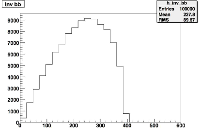
Figure 3: Parton level invariant mass distribution for $b$ quark pairs coming from gluino decays

In addition, the light and heavy neutral Higgs bosons h,H, as well as the A,should be easily accessible to the LHC through the $\gamma\gamma$, $\tau\tau$,and $\mu\mu$ decay channels. The lightest neutral Higgs boson is expected to be measured with a precision at the permille level, whereas the two heavy neutral Higgs bosons, essentially degenerate in mass, should be measurable with a precision of the order of 1-7% [52]. The charged Higgs bosons are observable in the $\tau\nu$-channel [60, 61]. While their observation will help discriminate between SUSY and non-SUSY models, the decay channel will not provide a precise mass measurement in this particular decay channel. Additionally, 50% of the total cross section, i.e., 10 pb, will be gluino pair production with a large branching ratio of about 25% for the gluino decay to $bb\tilde{\chi}_{2}^{0}$ . Thus one expects large rate of b-jets for this process which should be distinguishable from the standard model background. At the parton level, as shown in Figure 3, a clear edge can be observed for the invariant mass of $b$jet pairs providing information on the $\tilde{g}-\tilde{\chi}_{2}^{0}$  mass difference. The channel merits further investigation which is beyond the scope of this paper.

3 DETERMINATION OF THE mSUGRA PARAMETERS

To determine the errors on the underlying parameters from the measurements we use SFITTER [56, 55]. In a constrained model such as mSUGRA, five measurements are necessary to fit the fundamental parameters and determine their errors if we fix $\mu$ for example using the measurement of $(g-2)_{\mu}$ or the branching ratio for $B\to X_{s}\gamma$. In this case, the five measurements we use are: the masses of the three neutral Higgs bosons [74], the mass difference between the second-lightest and lightest neutralino and finally the mass difference between the gluino and second-lightest neutralino.

We explore two different strategies: First, we include only the systematic experimental errors (in the limit of high statistics), which are dominated by the limited knowledge of the energy scale of leptons (0.1%) and jets (1%) [75]. The results are shown in Table 3. The large unified scalar mass $m_{0}$ can be determined despite the absence of a direct measurement of slepton and squarks masses. While in the general MSSM the heavy Higgs boson mass A is a free parameter, in mSUGRA, the A mass as well as the H mass are sensitive to $\tan\beta$ as shown in Table 3. The supersymmetric particle measurements fix $m_{1/2}$.

The main source of uncertainty in the Higgs sector are parametric errors [75]. A shift in the bottom (top) quark mass of 0.05 GeV (1GeV) translates into a change of the heavy Higgs masses of 40 GeV (50 GeV). Once we include errors on top quark mass ($\pm 1$ GeV) and bottom quark mass ($\pm\leavevmode\nobreak\ 0.25$ GeV) and add theory errors (3 GeV on the Higgs boson masses, 1% on the neutralino mass difference, 3% on the gluino neutralino mass difference) we obtain the much larger errors shown in Table 3: All measurements are less precise by about an order of magnitude. In particular, the measurement of $m_{0}$ is seriously degraded, which makes it difficult or impossible to establish high-mass scalars. Most of this loss of precision is due to the lightest Higgs boson mass.

	nominal	exp errors	total error
$m_{0}$	1400	50	610
$m_{1/2}$	180	2.2	14
$\tan\beta$	51	0.3	4.6
$A_{0}$	700	200	687

Table 3: The nominal values and the errors on the fundamental parameters are shown for fits with experimental errors only, and total Error.

4 CONCLUSIONS

If supersymmetry should be realized with focus-point like properties, tri-leptons will be measured at the LHC with good precision. Adding mass measurements of the three neutral Higgs scalars, we dan determine the SUSY breaking parameters with good precision (assuming we know how SUSY is broken). Once we adds the parametric as well as theoretical errors, the precision decreases by an order of magnitude, and it will be difficult to establish heavy scalars with our limited set of measurements.

Acknowledgements

Lauren Tompkins would like to thank the Franco-American Fulbright Commission for financing her work and stay in France. In addition she would like to thank LAL Orsay and the ATLAS group for welcoming and supporting her as a member of the laboratory.

Part 6 Constraints on mSUGRA from indirect dark matter searches and the LHC discovery reach

V. Zhukov

1 INTRODUCTION

In the indirect Dark Matter (DM) search, the signal from DM annihilation can be observed as an excess of gamma, positron or anti-protons fluxes on top of the Cosmic Rays (CR) background, which is relatively small for these components. Existing experimental data on the diffusive gamma rays from the EGRET satellite and on positrons and anti-protons from the BESS, HEAT and CAPRICE balloon experiments show a significant excess of gamma with E${}_{\gamma}>$2 GeV and, to a lesser extent, of positrons and anti-protons in comparison with the conventional Galactic model (CM)  [76]. These excesses can be reduced, if one assumes that the locally measured spectra are different from the average galactic ones  [49]. This can be achieved by more than ten supernovae explosions in the vicinity of the solar system($\sim 100pc^{3}$) during last 10 Myr, which is at the statistical limit. An alternative explanation is annihilation of relic DM in the Galactic DM halo. The flux of i-component ($\gamma$, $e^{+}$, $\bar{p}$) from annihilation can be written as:
$F_{i}(E)\sim\frac{1}{m^{2}_{\chi}}\int\rho^{2}(r)B(r)G_{i}(E,\epsilon,r)\sum_{k}<\sigma_{k}v>A_{i}^{k}(\epsilon)drd\epsilon$,
where $<\sigma_{k}v>$ is the thermally averaged annihilation cross section into partons $k$, $A_{i}^{k}(\epsilon)$- hadronization of parton $k$ into the final state of $i$ component, $\rho(r)$ is the DM density distribution in the Galactic halo, $B(r)$ is the local clumpiness of the DM, or ’boost’ factor, $m_{\chi}$ is the mass of the DM particle and the $G_{i}(E,e,r)$ is the propagation term ($G_{\gamma}$=1). The annihilation cross section and the yield for each component can be calculated in the frame of the mSUGRA model where the DM particle is identified as a neutralino. The neutralino mass can be constrained by the shape of the gamma energy spectrum. The DM profile times boost factor $\rho^{2}(r)B(r)$ can be reconstructed from the angular distributions of the gamma excess [77]. The independent measurement of the galactic rotation curve can be used to decouple the bulk profile $\rho(r)$ and the clumpiness. The DM profile and the clumpiness are also connected to the cosmological scenario, in particular to the primary spectrum of density fluctuations[78]. The propagation of the annihilation products and the CR backgrounds can be calculated with a galactic model. In this study the DM annihilation was introduced into publicly available code of the GALPROP model  [79] and the simulated spectra have been compared with the experimental observations. Fig.1(left) shows the calculated annihilation yields and the ratio of the DM annihilation signal from the neutralino $m_{\chi}=55$ GeV to the CR fluxes for each component. The right hand side of the Fig.1 shows the EGRET diffusive gamma spectrum and the fluxes with and without DM annihilation.

In this analysis we discuss how the information from indirect DM search can be used to constrain the mSUGRA parameters and estimate the LHC potential in the defined region.

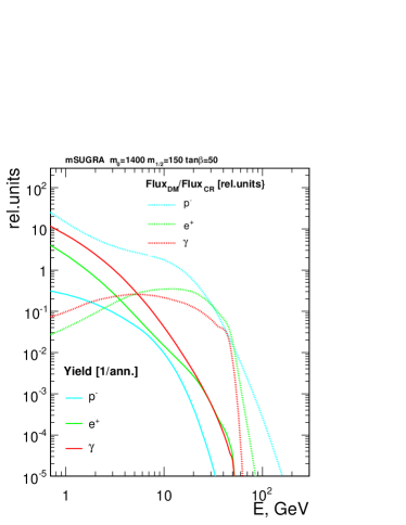
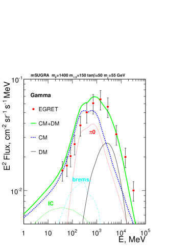
Figure 1: Left: The annihilation yields from neutralino ($m_{\chi}$=55 GeV) and the ratio of the fluxes from DM annihilation to the CR backgrounds after propagation. Right: The EGRET gamma spectrum and CR background calculated with and without DM contribution.

2 mSUGRA CONSTRAINTS

The current study is limited to the minimal supergravity (mSUGRA) model with universal scalar $m_{0}$ and gaugino $m_{1/2}$ masses at the GUT scale. The model is described by five well known parameters: $m_{0}$, $m_{1/2}$, tan$\beta$, $A_{0}$ and sgn($\mu$). The gluino and the neutralino-chargino mass spectrum at the EW scale are defined by $m_{1/2}$: $m_{\chi^{0}_{1}}\sim 0.4m_{1/2}$, $m_{\chi^{0}_{2}}\sim m_{\chi_{1}^{\pm}}\sim 0.8m_{1/2}$,$m_{\leavevmode\nobreak\ g}\sim 2.7m_{1/2}$ and $\sigma_{ann}\propto\frac{tan^{2}\beta}{m_{1/2}^{4}}$. The parameter space can be constrained by existing experimental data. The mass limits on the light Higgs boson ($m_{h}>114.3$ GeV) from LEP and the limit on $b\rightarrow s\gamma$ ([3.43$\pm$0.36] 10^-4) branching ratio from BaBar, CLOE and BELL constrain the low $m_{1/2}$ and $m_{0}$ region. The chargino mass ($m_{\chi_{1}^{\pm}}>103$ GeV) limits $m_{1/2}>150$ GeV for all $m_{0}$. For high $m_{0}$, the small $m_{1/2}$ region is excluded by the electroweak symmetry breaking (EWSB) requirements. The small value of tan$\beta<5$ can be excluded, if one assumes the unification of Yukawa couplings and top mass $m_{t}\sim$175 GeV [80]. The triliniar coupling $A_{0}$ is a free parameter. It can change significantly the interplay of different constraints, for example, at low or negative $A_{0}$, the $b\rightarrow s\gamma$ constraint overtakes the Higgs mass limits at low $m_{0}$. Further limitation on the parameter space can be obtained from the DM Relic Density(RD) of WMAP [81] $\Omega h^{2}=0.113\pm 0.009$. The RD was calculated with the micrOMEGAs1.4 [82] and the Suspect2.3.4  [62] and compared with the $\Omega h^{2}$. The evolution of the GUT parameters to the EW scale requires a solution to the RGE group equations, which is sensitive to the model parameters ($\alpha_{s}(M_{Z})(0.122),m_{b}(4.214),m_{t}(175)$, etc.), especially for high tan$\beta$ or the large $m_{0}$ region close to the EWSB limit  [83]. Using the RD constraint the mSUGRA $m_{0}-m_{1/2}$ plane can be divided between a few particular regions, according to the annihilation channel at the time of DM decoupling $T_{\chi}\sim\frac{m_{\chi}}{20}\sim$10 GeV. First of all, the lowest $m_{0}$ are excluded because LSP is the charged stau, not neutralino. Close to the forbidden region at low $m_{0}$ is the co-annihilation channel where the neutralino is almost mass-degenerate with staus. At low $m_{0}$ and $m_{1/2}$ annihilation goes via sfermions (mostly staus) in the t-channel with $\tau$ final state. In the A-channel the annihilation occurs via pseudoscalar Higgs A with a $b\bar{b}$ final state. The A-channel includes a resonance funnel region, where the allowed values of $m_{0}$, $m_{1/2}$ span the whole plane for different tan$\beta$, and the narrow region at small $m_{1/2}$ and $m_{0}>1000$, which appears only at large tan$\beta$. At large $m_{0}$, close to the EWSB limit, the annihilation also can happen via $Z$, $h$ and $H$ resonances. The RD constraint, including all these channels, shrinks the $m_{0}-m_{1/2}$ parameter space to a narrow band but only at fixed A₀ and tan$\beta$. The requirement to have a measurable signal from DM annihilation will also limit tan$\beta$. Indeed, nowadays at $T_{\chi}\sim$ 1.8K, only a few channels can produce enough signal. The annihilation cross section in $Z,H$ and $h$ channels depends on the momentum and is much smaller at present temperature. These channels, as well as the co-annihilation, will not contribute to the indirect DM signal. The $A$ channel and the staus exchange do not depend on the neutralino kinetic energy and have the same cross section as at decoupling $<\sigma v>\approx\frac{2\cdot 10^{-27}cm^{3}s^{-1}}{\Omega_{\chi}h^{2}}$. These two channels can produce enough signal although the energy spectrum of annihilation products is quite different, the $\tau$ decay producing much harder particles. The EGRET spectrum constrains $m_{\chi}$ in the 40-100 GeV range, or $m_{1/2}$=100-250 GeV [77]. Since the gamma rays from the $\tau$ decay are almost 10 times harder, only the A-channel at low $m_{1/2}$ can reproduce the shape of the EGRET excess. Fig. 2 shows on the left the $m_{0}-m_{1/2}$ region compatible with the EGRET data and different constraints. The scatter plot of Fig. 2(right) shows models compatible with the RD at different tan$\beta$. The RD is compatible with low $m_{1/2}$ for the A -channel only at relatively large tan$\beta=50-60$. This limits the mSUGRA parameters to the $m_{1/2}$=150-250 GeV, $m_{0}$=1200-2500 GeV and tan$\beta$=50-60. The obtained limits depend on the ’boost’ factor. which was found to be in the range of $5-50$ for all components (depending on the DM profile), this is compatible with the cosmological simulations [78]. The larger ’boost’ factor above 10³ will allow contribution from the resonance and co-annihilation channels and the tan$\beta$ constraint will be relaxed.

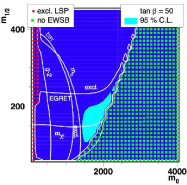
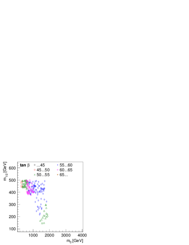
Figure 2: Left: different constraints of mSUGRA parameters (tan$\beta$=50, A₀=0) and the region (blue) allowed by the gamma data. Right: random scan of tan$\beta$ for the models compatible with the RD constraints.

3 SIGNATURES AT THE LHC

The relatively large $m_{0}$ and low $m_{1/2}$ region favored by the indirect DM search can be observed at the LHC energy $\sqrt{s}=14$ TeV. The dominant channel is the gluino production with a subsequent cascade decay into neutralinos ($\chi_{2}^{0}$, $\chi_{3}^{0}$) and chargino $\chi_{1}^{\pm}$. The direct production of the neutralino-chargino $\chi_{2}^{0}$ + $\chi_{1}^{\pm}$ pairs also has a significant cross section at low $m_{1/2}$. In both cases the main discovery signature is the invariant mass distribution of two opposite sign same flavor(OSSF) leptons ($e$ or $\mu$) produced from three body decay of neutralino $\chi_{2}^{0}\rightarrow\chi_{1}^{0}l^{+}l^{-}$. This distribution has a particular triangular shape with the kinematic end point $M_{ll}^{max}$=$m_{\chi_{2}^{0}}-m_{\chi_{1}^{0}}$. Fig. 3 shows event topologies for the gluino and gaugino channels. The main final state for the gluino production is the 2OSSF leptons plus jets and a missing transverse energy (MET). For the neutralino-chargino production it is the pure trilepton state without central jets.

We have studied the discovery reach of the CMS detector for these channels using the fast simulation (FAMOS), verified with the smaller samples produced in full GEANT model (ORCA). The signal and backgrounds have been generated with PYTHIA6.225 and ISASUGRA7.69 at leading order (LO), the NLO corrections have been taken into account by multiplying with the $K_{NLO}$ factor. The low luminosity pileup has been included. The selection of events have been done in two steps; 1) the sequential cuts were applied to the reconstructed events, 2) the selected samples were passed through the Neural Network (NN). The NN was trained separately for each signal-background pair and the cuts on the NN outputs have been optimized for the maximum significance. The LM9 CMS benchmark point ($m_{0}$=1450, $m_{1/2}$=175, tan$\beta$=50, A₀=0) was used as a reference in this study.

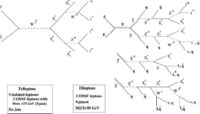
Figure 3: Events topology at the LHC for the mSUGRA region compatible with the indirect DM search ($m_{1/2}<$250 and $m_{0}>1000$ GeV)

For the gluino decay the main backgrounds are coming from the $t\bar{t}$, Z+jets(here $\hat{p}>20$ GeV) and inclusive SUSY(LM9) channels. The selection cuts require at least 2 OSSF isolated leptons with $P_{T}^{\mu}>$10 GeV/c($P_{T}^{e}>$15 GeV/c) for muons(electrons), more than 4 central ($|\eta|<2.4$) jets with $E_{T}>$30 GeV and the missing transverse energy $MET>$50 GeV. The NN was trained with the following variables: $N_{jets}$, $E_{T}^{jeth}$, $\eta_{jeth}$, $M_{ll}$, $MET$, $\sum E_{T}$, $P_{T}^{3}$,$\frac{P_{T}^{l1}-P_{T}^{l2}}{P_{T}^{l1}+P_{T}^{l2}}$. The NN orders the variables according to the significance for each signal-background combination. The dilepton invariant mass for all OSSF combinations after all selections is shown on the left side of Fig. 4 for the LM9 point. The events, which has invariant masses close to the Z peak ($M_{ll}>75$ GeV), have been excluded. The significance $S_{cp}$=23 is expected for an integrated luminosity 30 fb^-1. The discovery region compatible with the EGRET, is shown on the right hand side of the Fig. 4. The scan was limited to $m_{1/2}>150$ GeV due to constraints on the chargino mass. The gluino channel has more other signal signatures which can provide even better background separation and this estimation should be considered as a low limit.

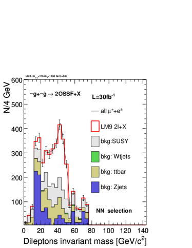
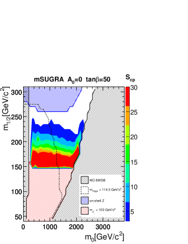
Figure 4: Left: Invariant mass of all OSSF lepton pairs for the mSUGRA gluino decays into at least one $\chi_{2}^{0}$ for the CMS LM9 point ($m_{0}$=1450, $m_{1/2}$=175, tan$\beta$=50, A₀=0). Right: Discovery reach in $m_{0},m_{1/2}$ plane at tan$\beta$=50 for $L_{int}$=30 fb^-1, the significance S_cp is shown as a color grades.

For the direct neutralino-chargino production $\chi^{0}_{2}\chi^{\pm}_{1}$ the trilepton final state was selected using the following criteria: no central jets ($E_{T}>30$GeV and $\eta<2.4$), two OSSF isolated leptons ($P_{T}^{\mu}>$10 GeV/c, $P_{T}^{e}>$15 GeV/c ) plus any lepton with $P_{T}^{l}>10$ GeV/c, see Fig. 3. The MET cut, very effective for the background suppression in other SUSY channels, fails here as the gauginos are light at $m_{1/2}<250$ GeV. The main background comes from Z+jets, Drell Yan, $t\bar{t}$ and ZW/ZZ production. The NN was trained with the variables: $\sum P_{T}$, P${}_{T}^{1,2,3}$, $\Theta_{ll}$, $P_{T}^{3}$,$\frac{P_{T}^{l1}-P_{T}^{l2}}{P_{T}^{l1}+P_{T}^{l2}}$, $M_{ll}$, $MET$. The expected significance of the trilepton final state for the LM9 point is $S_{cp}$=6.1 for $L_{int}$=30 fb^-1 at low luminosity, see Fig. 5. At high luminosity the jets veto selection can reduce the signal selection efficiency by $\sim 30\%$ and another selection cuts are needed. The right hand side of Fig. 5 shows the discovery reach of the trilepton final state.

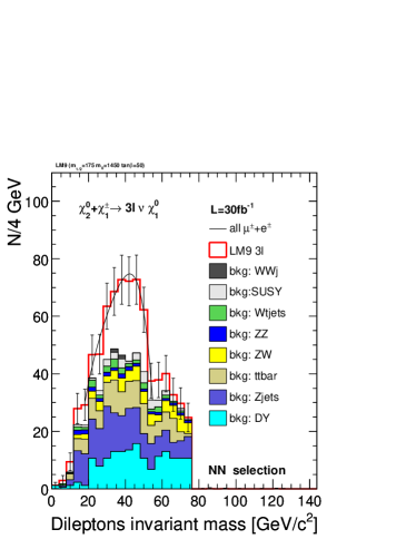
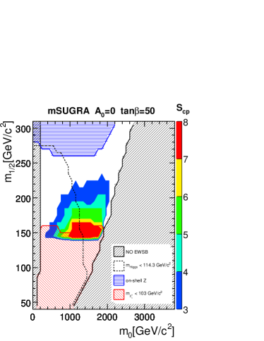
Figure 5: Left: Invariant mass of all OSSF lepton pairs for the mSUGRA trilepton at the CMS LM9 point($m_{0}$=1450, $m_{1/2}$=175, tan$\beta$=50, A₀=0). Right: Discovery reach in $m_{0},m_{1/2}$ plane at tan$\beta$=50 for $L_{int}$=30 fb^-1, the significance S_cp is shown as a color grades.

Both channels, in spite of different event topology, have overlapping discovery regions and are compatible with the region defined from indirect DM search.

4 CONCLUSIONS

The existing experimental data from the indirect DM search, together with the electroweak and relic density constraints, limit the mSUGRA parameters to a narrow region $m_{1/2}\sim$150-250 GeV, $m_{0}\sim$1200-2500 GeV and tan$\beta\sim$50-60. The LHC will probe this region at integrated luminosity $L_{int}>$30 fb^-1. The main discovery channels are the gluino decay into $m_{\chi^{0}_{2}}$ with 2OSSF dilepton plus jets final state and the neutralino-chargino direct production with the pure trilepton final state.

Acknowledgements

I would like to thanks my collaborators at Karlsruhe University W. de Boer, C. Sander, M. Niegel who share all results and T. Lari, A. Pukhov, M. Galanti, D. Kazakov for usefull discussions during and after the workshop.

Part 7 Relic density of dark matter in the MSSM with CP violation

G. Bélanger, F. Boudjema, S. Kraml, A. Pukhov and A. Semenov

1 INTRODUCTION

One of the interest of supersymmetric models with R-parity conservation is that they provide a natural cold dark matter candidate, the lightest supersymmetric particle (LSP). The precise measurement of the relic density of dark matter by WMAP, $0.0945<\Omega h^{2}<0.1287$ [2, 3] now strongly constrains the parameter space of supersymmetric models. Such is the case for example in mSUGRA models, where the relic density of dark matter is often too large [8, 84, 85, 86, 87, 88, 4]. It has been pointed out that if one allows the parameters of the MSSM to be complex, the relic density could be modified, even opening up new allowed regions of parameter space [89, 90]. Furthermore, the issue of CP violation in the MSSM is also interesting from the cosmological point of view as it provides a possible solution to the baryon number asymmetry via the electroweak baryogenesis mechanism [91]. As a first step towards a comprehensive study of the relic density of dark matter in the MSSM with CP violation, we present here some results for the case where the neutralino is the LSP and annihilates dominantly through heavy Higgs exchange.

2 THE MODEL

We consider the general MSSM with parameters defined at the weak scale. In general, one can have complex parameters in the neutralino/chargino sector with $M_{i}=|M_{i}|e^{i\phi_{i}}$, $\mu=|\mu|e^{i\phi_{\mu}}$ as well as for the trilinear couplings, $A_{f}=|A_{f}|e^{i\phi_{f}}$. The phase of $M_{2}$ can be rotated away. Among the trilinear couplings, $A_{t}$ has the largest effect on the Higgs sector. Morever as the phase of $\mu$ is the most severely constrained by electric dipole moment (EDM) measurements, we set it to zero and consider only the two remaining phases, $\phi_{1}$ and $\phi_{t}$.

In the MSSM, the Higgs sector consists of two CP-even states $h^{0},H^{0}$ and one CP odd state $A$. Adding CP violating phases in the model induces mixing between these three states. The mass eigenstates $h_{1},h_{2},h_{3}$ ($m_{h_{1}}<m_{h_{2}}<m_{h_{3}}$) are no longer eigenstates of CP. The mixing matrix is defined by

$$(\phi_{1},\phi_{2},a)^{T}_{a}=H_{ai}(h_{1},h_{2},h_{3})_{i}^{T}.$$ (1)

In what follows we will mainly be concerned with the coupling of the lightest neutralino to Higgses that govern the neutralino annihilation cross sections via Higgs exchange. The Lagrangian for such interactions writes

$${\cal L}_{{\tilde{\chi}^{0}_{1}}{\tilde{\chi}^{0}_{1}}h_{i}}=\frac{g}{2}{\sum_{i=1}^{3}}\overline{\tilde{\chi}_{1}^{0}}(g^{S}_{h_{i}{\tilde{\chi}^{0}_{1}}{\tilde{\chi}^{0}_{1}}}+i\gamma_{5}g^{P}_{h_{i}{\tilde{\chi}^{0}_{1}}{\tilde{\chi}^{0}_{1}}})\tilde{\chi}_{1}^{0}h_{i}$$ (2)

with the scalar part of the coupling

$$g^{S}_{h_{i}{\tilde{\chi}^{0}_{1}}{\tilde{\chi}^{0}_{1}}}=Re\left[(N_{12}^{*}-t_{W}N_{11}^{*})\left(H_{1i}N_{13}^{*}-H_{2i}N_{14}^{*}-iH_{3i}(s_{\beta}N_{13}^{*}-c_{\beta}N_{14}^{*})\right)\right],$$ (3)

where $N$ is the neutralino mixing matrix in the SLHA notation [92]. The pseudoscalar component $g^{P}_{h_{i}{\tilde{\chi}^{0}_{1}}{\tilde{\chi}^{0}_{1}}}$ corresponds to the imaginary part of the same expression. The LSP couplings to Higgses will clearly be affected both by phases in the neutralino sector, for example $\phi_{1}$, which modifies the neutralino mixing, as well as from phases that enter the Higgs mixing. The latter can for example result from introducing a phase in the trilinear coupling $A_{t}$. Indeed in the MSSM the mixing is induced by loops involving top squarks and is proportional to $Im(A_{t}\mu)/(m^{2}_{{\tilde{t}}_{2}}-m^{2}_{{\tilde{t}}_{1}})$ [93]. Thus a large mixing is expected when $Im(A_{t}\mu)$ is comparable to the squared of the stop masses. Note that the masses of the physical Higgses also depend on the phase of $A_{t}$. In particular larger mass splitting between heavy Higgses are found for large values of $\mu A_{t}$.

3 RELIC DENSITY OF DARK MATTER

The computation of the relic density of dark matter in supersymmetric models is now standard, and public codes are available which perform this calculation either in the context of the MSSM or of a unified model. Here we are using an extension of micrOMEGAs [6, 5] that allows for complex parameters in the MSSM  [94]. Using LanHEP [95], a new MSSM model file with complex parameters was rebuilt in the CalcHEP  [96] notation, thus specifying all relevant Feynman rules. For the Higgs sector, an effective potential is written in order to include in a consistent way higher-order effects. Masses, mixing matrices and parameters of the effective potential are read directly from CPsuperH [97] as well as masses and mixings of neutralinos, charginos and third generation sfermions. On the other hand masses of the first two generations of sfermions are computed at tree-level from the input parameters of the MSSM at the weak scale. All cross sections for annihilation and coannihilation processes are computed automatically with CalcHEP, and the standard micrOMEGAs  routines are used to calculate the effective annihilation cross section and the relic density of dark matter.

The cross sections for some of the annihilation and coannihilation processes will depend on phases, and so will the thermally-averaged cross section. At the same time, the phases change the physical masses and so can strongly impact the value of the relic density, especially when coannihilation processes are important or when annihilation occurs near a resonance. It is the latter case that we will consider in more details here.

At vanishing relative velocity, $v$, neutralino annnihilation through s-channel exchange is p-wave suppressed; the annihilation proceeds strictly through pseudoscalar exchange. Nevertheless when performing the thermal averaging, the scalar exchange cannot be neglected altogether. In the MSSM with real parameters it can amount to ${\cal O}(10\%)$ of the total contribution. In the presence of phases both heavy Higgses can acquire a pseudoscalar component (that is $g^{P}_{h_{i}{\tilde{\chi}^{0}_{1}}{\tilde{\chi}^{0}_{1}}}\neq 0$) and so both $h_{2}$ and $h_{3}$ can significantly contribute to neutralino annihilation even at small $v$. There is a kind of sum rule that relates the couplings squared of the Higgses to neutralinos. Therefore, for the two heavy eigenstates which are in general close in mass, we do not expect a large effect on the resulting relic density from Higgs mixing alone. A noteworthy exception occurs when, for kinematical reason, only one of the two resonances is accessible in neutralino annihilation, that is $m_{h_{2}}<m_{{\tilde{\chi}^{0}_{1}}}<m_{h_{3}}$.

4 RESULTS

In order not to vary too many parameters, we choose, $M_{1}=150{\rm\;GeV},M_{2}=300{\rm\;GeV},\tan\beta=5$, $M_{Q_{3},U_{3},D_{3}}=500{\rm\;GeV}$ and $A_{t}=1200{\rm\;GeV}$. EDM constraints are avoided by setting $\phi_{\mu}=0$ and pushing the masses of the 1st and 2nd generation sfermions to $10{\rm\;TeV}$. We consider two scenarios, $\mu=500{\rm\;GeV}$ and $\mu=1{\rm\;TeV}$ leading to small and large mixing in the Higgs sector respectively for $\phi_{t}\neq 0$. In both cases the LSP is dominantly bino. As mentioned above, allowing for non-zero phases not only affects the neutralino and Higgs couplings but also their physical masses. Since the relic density is very sensitive to the mass difference $\Delta m_{{\tilde{\chi}^{0}_{1}}h_{i}}=m_{h_{i}}-2{m_{\tilde{\chi}^{0}_{1}}}$  [98, 83], it is important to disentangle the phase effects in kinematics and in couplings. As we will see, a large part of the huge phase effects reported in Ref. [99] can actually be attributed to a change in $\Delta m_{{\tilde{\chi}^{0}_{1}}h_{i}}=m_{h_{i}}-2{m_{\tilde{\chi}^{0}_{1}}}$.

4.1 Scenario 1: small Higgs mixing

In the first scenario we fix $\mu=500{\rm\;GeV}$ so that there is small Higgs mixing. Details of the mass spectrum are shown in Table 1. The mass of the charged Higgs, $m_{H^{+}}=340{\rm\;GeV}$, is chosen such that for real parameters the relic density falls within the WMAP range, $\Omega h^{2}=0.11$. In this case, when the parameters are real, $h_{2}$ is the pseudoscalar. The main channel for annihilation of neutralinos are then characterictic of $h_{2}$ branching fractions, which goes predominantly into fermion pairs, $b\bar{b}$ (78%), $\tau\bar{\tau}$ (10%) with a small contribution from the light Higgs channels $Zh_{1}$ (7%). When we vary either the phases of $A_{t}$ or of $M_{1}$, we observe large shifts in the relic density.

First consider varying the phase $\phi_{t}$, which affects the stop sector as well as the Higgs masses and mixings through loop effects. In this scenario with $\mu$ small, the scalar-pseudoscalar mixing never exceeds 8%. We show that the phase dependence is directly linked to the mass dependence of the $h_{2}$ which is predominantly pseudoscalar. In Fig. 1 we plot the band that is allowed by WMAP in the $m_{H}^{+}-\phi_{t}$ plane. One can see that lower and upper WMAP bounds correspond to the contours for $\Delta m_{{\tilde{\chi}^{0}_{1}}h_{2}}=36.2$ and $38.6{\rm\;GeV}$ respectively with only $4\%$ deviation. So the main effect of $\phi_{t}$ can be explained by shifts in the physical masses and position of the resonance.

 

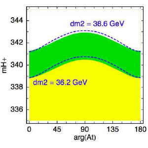
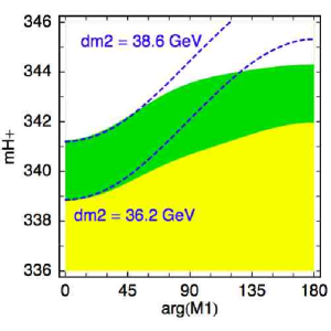
Figure 1: The WMAP allowed bands (green/dark grey) in the a) $m_{H^{+}}-\phi_{t}$ and b) $m_{H^{+}}-\phi_{1}$ plane for Scenario 1. Contours of constant mass differences ${\rm dm2}=\Delta m_{{\tilde{\chi}^{0}_{1}}h_{2}}$ are also displayed. In the yellow (light grey) region $\Omega h^{2}$ is below the WMAP range.

We next vary the phase $\phi_{1}$, keeping $\phi_{t}=0$. This phase changes the neutralino masses and mixings, which in turn determine the couplings of neutralinos to Higgses, Eq. 3. For $m_{H^{+}}=340{\rm\;GeV}$, when increasing $\phi_{1}$, the relic density drops, see Fig. 1b. This is because the mass of the neutralino increases slowly, resulting in a smaller $\Delta m_{{\tilde{\chi}^{0}_{1}}h_{2}}$. If one readjusts either the mass of the neutralino or the mass of the Higgs to have a constant mass difference, we find rather that the relic density increases with $\phi_{1}$. The reason is that for $\phi_{1}=0$ $(g^{S},g^{P})_{h_{2}{\tilde{\chi}^{0}_{1}}{\tilde{\chi}^{0}_{1}}}=(10^{-5},-.056)$ and $(g^{S},g^{P})_{h_{3}{\tilde{\chi}^{0}_{1}}{\tilde{\chi}^{0}_{1}}}=(-.045,10^{-5})$, while for $\phi_{1}=90^{\circ}$, $(g^{S},g^{P})_{h_{2}{\tilde{\chi}^{0}_{1}}{\tilde{\chi}^{0}_{1}}}=(0.047,-.008)$ and $(g^{S},g^{P})_{h_{3}{\tilde{\chi}^{0}_{1}}{\tilde{\chi}^{0}_{1}}}=(-.002,0.043)$. Therefore for $\phi_{1}=0$, $h_{2}$ exchange dominates with a large cross section while for $\phi_{1}=90^{\circ}$ one gets about equal contribution from $h_{2}$ and $h_{3}$ although with a smaller overall cross section. When increasing $\phi_{1}$ further (up to $180^{\circ}$), $h_{2}$ exchange again dominates, however with a coupling to neutralinos smaller by 30% than for $\phi_{1}=0$. Thus one needs a smaller mass splitting $\Delta m_{{\tilde{\chi}^{0}_{1}}h_{2}}$ for $\Omega h^{2}$ to fall within the WMAP range, see Fig. 1b. Moreover, for large phases there is also a sizeable contribution from ${\tilde{\chi}^{0}_{1}}{\tilde{\chi}^{0}_{1}}\rightarrow h_{1}h_{1}$ with a constructive interference between s-channel $h_{3}$ and t-channel neutralino exchange. In Fig. 2 we show the variation of $\Omega h^{2}$ with $\phi_{1}$ while keeping $\Delta m_{{\tilde{\chi}^{0}_{1}}h_{2}}$ fixed. The maximum deviation, which is purely an effect due to shifts in couplings, can reach 50%.

Figure 2: $\Omega h^{2}$ as a function of $\phi_{1}$ in Scenario 1. The value of $M_{1}$ is adjusted so that $\Delta m_{{\tilde{\chi}^{0}_{1}}h_{2}}$ stays constant. The green (grey) band corresponds to the $2\sigma$ WMAP range.

Scenario 1, $\phi_{t}=0$
	$m_{H^{+}}=340$
$\phi_{1}$	0	90	180
${\tilde{\chi}^{0}_{1}}$	147.0	148.7	150.3
$m_{h_{2}}$	331.5	331.5	331.5
$m_{h_{3}}$	332.3	332.3	332.3
$\Omega h^{2}$	0.11	0.087	0.072

Scenario 2, $\phi_{1}=0$
	$m_{H^{+}}=334$		$m_{H^{+}}=305$
$\phi_{t}$	0	90	0	90
${\tilde{\chi}^{0}_{1}}$	149.0	149.0	149.0	149.0
$m_{h_{2}}$	324.4	318.4	294.7	288.2
$m_{h_{3}}$	326.2	328.9	296.5	299.5
$\Omega h^{2}$	0.125	0.044	0.107	0.064

Table 1: Examples of LSP and Higgs masses (in GeV) and the resulting $\Omega h^{2}$ for the two scenarios considered.

4.2 Scenario 2: large Higgs mixing

As second case, we consider a scenario with a large mixing in the Higgs sector. For this we fix $\mu=1$ TeV. All other parameters have the same values as in the first scenario safe for the charged Higgs mass which is set to $m_{H^{+}}=334{\rm\;GeV}$ such that for real parameters the value of the relic density agrees with WMAP, $\Omega h^{2}=0.125$. This mass is lower than in the previous scenario because the Higgsino fraction of the LSP is smaller, so one needs to be closer to the Higgs resonance. For $\phi_{t}\neq 0$ we have a large pseudoscalar/scalar mixing and hence a stronger dependence of $\Omega h^{2}$ on $\phi_{t}$. For $\phi_{t}=0$, $h_{3}$ is the pseudoscalar and gives the dominant contribution to neutralino annihilation while for $\phi_{t}=90^{\circ}$ $h_{2}$ is the pseudoscalar, hence giving the dominant contribution. Consequently in Fig. 3, agreement with WMAP is reached for $\Delta m_{{\tilde{\chi}^{0}_{1}}h_{i}}\sim 25{\rm\;GeV}$ with $h_{i}=h_{3}$ at $\phi_{t}=0$ and $180^{\circ}$, and $h_{i}=h_{2}$ at $\phi_{t}=90^{\circ}$.

 

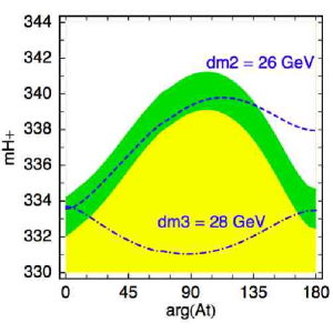
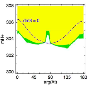
Figure 3: The WMAP allowed bands (green/dark grey) in the $m_{H^{+}}-\phi_{t}$ plane for scenario 2 with a) $m_{H^{+}}\sim 335{\rm\;GeV}$ and b) $m_{H^{+}}\sim 305{\rm\;GeV}$ . Contours of constant mass differences ${\rm dmi}=\Delta m_{{\tilde{\chi}^{0}_{1}}h_{i}}$ are also displayed. In the yellow (light grey) region $\Omega h^{2}$ is below the WMAP range.

When the neutralino mass is very near the two heavy Higgs resonances, one finds another region where the relic density falls within the WMAP range. In the real case one needs $m_{H^{+}}=305$ GeV, giving a mass difference $\Delta m_{{\tilde{\chi}^{0}_{1}}h_{3}}=-1.5{\rm\;GeV}$. Note that annihilation is efficient enough even though one catches only the tail of the pseudoscalar resonance. For the same charged Higgs mass, the mass of $h_{3}$ increases when one increases $\phi_{t}$, so that neutralino annihilation becomes more efficient despite the fact that $h_{3}$ becomes scalar-like and $g^{p}_{{\tilde{\chi}^{0}_{1}}{\tilde{\chi}^{0}_{1}}h_{3}}$ decreases. When $\phi_{t}\sim 75^{\circ}-90^{\circ}$, the coupling $g^{p}_{{\tilde{\chi}^{0}_{1}}{\tilde{\chi}^{0}_{1}}h_{3}}$ becomes very small and one needs $\Delta m_{{\tilde{\chi}^{0}_{1}}h_{3}}=0-1.5{\rm\;GeV}$ to achieve agreement with WMAP, see Fig. 3b. Here we are in the special case where $m_{h_{2}}<2m_{{\tilde{\chi}^{0}_{1}}}\leq m_{h_{3}}$, so that only $h_{3}$ contributes significantly to the relic density. This feature is very specific to this choice of parameters. Even for constant values of $\Delta m_{{\tilde{\chi}^{0}_{1}}h_{3}}=-1.5{\rm\;GeV}$ we get an increase in $\Omega h^{2}$ relative to the $\phi_{t}=0$ case by almost an order of magnitude. This is however far less than the shifts of two orders of magnitude found for fixed values of $m_{H^{+}}$. Note that there is also a small contribution from $h_{2}$ exchange but no significant interference with t-channel diagrams.

5 CONCLUSIONS

The predictions for the relic density of dark matter in the MSSM with CP violation can differ significantly from the ones in the CP conserving case. Some of these effects are simply due to shifts in neutralino and/or Higgs masses. However, one also has phase dependences due to shifts in the couplings of neutralinos and Higgs as well as, in specific cases, due to interferences between several contributions. Removing kinematical effects, we find a maximal deviation of $\Omega h^{2}$ of one order of magnitude. We have here only showed results for the case where the neutralinos annihilate via Higgs exchange. A systematic investigation of the different scenarios of neutralino annihilation (the cases of wino, Higgsino or mixed gaugino-Higgsino LSP, as well as the case of coannihilation with stops or staus) including CP violation is underway.

Acknowledgements

We thank J.S. Lee for his help with CPsuperH and W. Porod for discussions. This work was supported in part by GDRI-ACPP of CNRS and by grants from the Russian Federal Agency for Science, NS-1685.2003.2 and RFBR-04-02-17448. A. P. acknowledges the hospitality of CERN and LAPTH where some of the work contained here was performed. S.K. is supported by an APART (Austrian Programme for Advanced Research and Technology) grant of the Austrian Academy of Sciences. She also acknowledges the financial support of CERN for the participation at the Les Houches Workshop.

Part 8 Light scalar top quarks

C. Balázs^∗, M. Carena, A. Finch, A. Freitas, S. Kraml, T. Lari, A. Menon, C. Milsténe, S. Moretti, D.E. Morrissey, H. Nowak, G. Polesello, A.R. Raklev, C.H. Shepherd-Themistocleous, A. Sopczak^∗ and C.E.M. Wagner
^∗ editors of this part.

1 INTRODUCTION

Most of the matter in the Universe consists of baryons and non-luminous (dark) matter. The amount of these components are typically predicted independently from each other. In this section, we discuss the collider implications of a supersymmetric scenario that provides a common origin for both major components of matter. A cornerstone of this scenario is the assumption that the baryon asymmetry of the Universe is generated via electroweak baryogenesis. This assumption, in its minimal form, leads to a light scalar top quark, 100 GeV $\;\raisebox{-3.87495pt}{$\textstyle\stackrel{{\scriptstyle\textstyle<}}{{\sim}}$}\;m_{{\tilde{t}}_{1}}\;\raisebox{-3.87495pt}{$\textstyle\stackrel{{\scriptstyle\textstyle<}}{{\sim}}$}\;m_{t}$. If this light scalar top is found at colliders it can be a smoking gun signature of electroweak baryogenesis.

After highlighting the basics and the consequences of the electroweak baryogenesis mechanism in the Minimal Supersymmetric extension of the Standard Model (MSSM), in section 2 the viability that the MSSM simultaneously provides the measured baryon asymmetry and dark matter abundance is summarized.

Then, in section 3 a new method is presented to discover a baryogenesis motivated light scalar top, decaying dominantly into $c\tilde{\chi}^{0}_{1}$, at the LHC. The principal idea is to exploit the Majorana nature of the gluino, which implies that gluinos do not distinguish between $t\tilde{t}_{1}^{*}$ and $\bar{t}\tilde{t}_{1}$ combinations. This leads to like-sign top quarks in events of gluino pair production followed by gluino decays into top and stop.

This is followed by section 4 where a detailed analysis based on a parametrized simulation of the ATLAS detector is presented. A benchmark model is studied in the framework of the MSSM, with a scalar top quark lighter than the top quark, yielding a final state similar to the one for $t\bar{t}$ production. It is demonstrated that a signal for the stop can be extracted in this case, and the kinematic features of the stop decay can be studied. A technique to subtract the Standard Model background based on the data is developed to achieve this result.

If scalar tops are light enough and are subject to large mixing effects, in the context of the MSSM, they may be produced at the LHC in pairs and in association with the lightest Higgs boson (decaying into bottom quark pairs). For the case in which top squarks are lighter than top quarks, they typically decay into charmed quarks and undetectable neutralinos. Thus the overall emerging signature is naturally composed of four isolated jets, two of which may be tagged as $b$-jets and two as $c$-jets, accompanied by sizable missing transverse energy. Two MSSM scenarios are considered in section 5, for which we investigate the behaviour of kinematic variables that could possibly be employed in the experimental selection of such events.

Finally, scalar top quark studies at a Linear collider are presented in section 6. The cosmologically interesting scenario with small mass difference between the scalar top and the neutralino has been addressed in particular. The ILC will be able to explore this region efficiently. The simulation is based on a fast and realistic detector simulation. The scenario of small mass differences is a challenge for c-quark tagging with a vertex detector. A vertex detector concept of the Linear Collider Flavor Identification (LCFI) collaboration, which studies CCD detectors for quark flavor identification, is implemented in the simulations. The study extends simulations for large mass differences (large visible energy).

2 BARYOGENSIS AND DARK MATTER

2.1 Overview of electroweak baryogenesis

The cosmological energy density of both main components of matter, baryons and dark matter, is known with a remarkable precision. Recent improvements of the astrophysical and cosmological data, most notably due to the Wilkinson Microwave Anisotropy Probe (WMAP) [3], have determined the baryon density of the Universe (in units of the critical density $\rho_{c}=3H_{0}^{2}/(8\pi G_{N})$) to be

$$\Omega_{B}h^{2}=0.0224\pm{0.0009},$$ (1)

with $h=0.71^{+0.04}_{-0.03}$. (Here $H_{0}=h\times 100\leavevmode\nobreak\ km/s/Mpc$ is the present value of the Hubble constant, and $G_{N}$ is Newton’s constant.) According to the observations, the baryon density is dominated by baryons while anti-baryons are only secondary products in high energy processes. The source of this baryon–anti-baryon asymmetry is one of the major puzzles of particle physics and cosmology.

Assuming that inflation washes out any initial baryon asymmetry after the Big Bang, there should be a dynamic mechanism to generate the asymmetry after inflation. Any microscopic mechanism for baryogenesis must fulfill the three Sakharov requirements [100]:

• baryon number (B) violation,

• CP violation, and

• departure from equilibrium (unless CPT is violated [101]).

All three requirements are satisfied in both the SM and the MSSM during the electroweak phase transition. This is the basis for electroweak baryogenesis (EWBG) [102, 103, 104, 105, 106]. While electroweak baryogenesis is viable in the MSSM, SM processes cannot generate a large enough baryon asymmetry during the electroweak phase transition.

Baryon number violation occurs in the SM and the MSSM due to quantum transitions between inequivalent SU(2) vacua that violate $(B\!+\!L)$ [107]. These transitions are exponentially suppressed at low temperatures in the electroweak broken phase [108, 109], but become active at high temperatures when the electroweak symmetry is restored [110, 111, 112, 113, 114]. In the absence of other charge asymmetries, like $(B\!-\!L)$, they produce baryons and anti-baryons such that the net baryon number relaxes to zero, and so do not by themselves generate a baryon asymmetry [115].

If the electroweak phase transition is first order, bubbles of broken phase nucleate within the symmetric phase as the Universe cools below the critical temperature. These provide the necessary departure from equilibrium. EWBG then proceeds as follows [116]. CP violating interactions in the bubble walls generate chiral charge asymmetries which diffuse into the symmetric phase in front of the walls. There, sphaleron transitions, which are active in the symmetric phase, convert these asymmetries into a net baryon number. This baryon number then diffuses into the bubbles where the electroweak symmetry is broken. The chiral charges produced in the bubble wall are able to diffuse into the symmetric phase, where they are approximately conserved, but not into the broken phase, where they are not.

Sphaleron transitions within the broken phase tend to destroy the baryon number generated outside the bubble. To avoid this, the sphaleron transitions within the broken phase must be strongly suppressed. This is the case provided the electroweak phase transition is strongly first order [117],

$$v(T_{c})/T_{c}\;\raisebox{-3.87495pt}{$\textstyle\stackrel{{\scriptstyle\textstyle>}}{{\sim}}$}\;1,$$ (2)

where $v(T_{c})$ denotes the Higgs vacuum expectation value at the critical temperature $T_{c}$.

The strength of the electroweak phase transition may be determined by examining the finite temperature effective Higgs boson potential. The Higgs vacuum expectation value at the critical temperature is inversely proportional to the Higgs quartic coupling, related to the Higgs mass. For sufficiently light Higgs bosons, a first-order phase transition can be induced by the loop effects of light bosonic particles, with masses of the order of the weak scale and large couplings to the Higgs fields. The only such particles in the SM are the gauge bosons, and their couplings are not strong enough to induce a first-order phase transition for a Higgs mass above the LEP-2 bound [118, 119, 120].

Within the MSSM, there are additional bosonic degrees of freedom which can make the phase transition more strongly first-order. The most important contribution comes from a light stop, which interacts with the Higgs field with a coupling equal to the top-quark Yukawa. In addition, a light stop has six degrees of freedom, three of colour and two of charge, which further enhances the effect on the Higgs potential. Detailed calculations show that for the mechanism of electroweak baryogenesis to work, the lightest stop mass must be less than the top mass but greater than about 120 GeV to avoid colour-breaking minima. Simultaneously, the Higgs boson involved in breaking the electroweak symmetry must be lighter than 120 GeV [121, 122, 123, 124, 125, 126, 127, 128, 129, 130, 131, 132], and only slightly above the present experimental bound [133],

$$m_{h}\;\raisebox{-3.87495pt}{$\textstyle\stackrel{{\scriptstyle\textstyle>}}{{\sim}}$}\;114\leavevmode\nobreak\ \mbox{GeV},$$ (3)

which is valid for a SM Higgs boson.

The combined requirements of a first-order electroweak phase transition, strong enough for EWBG, and a Higgs boson mass above the experimental limit severely restrict the allowed values of the stop parameters. To avoid generating too large a contribution to $\Delta\rho$, the light stop must be mostly right-handed. Since the stops generate the most important radiative contribution to the Higgs boson mass in the MSSM [134, 135, 136], the other stop must be considerably heavier in order to raise the Higgs boson mass above the experimental bound, Eq. (3). For the stop soft supersymmetry breaking masses, this implies [127]

$$m_{U_{3}}^{2}\;\raisebox{-3.87495pt}{$\textstyle\stackrel{{\scriptstyle\textstyle<}}{{\sim}}$}\;0,$$ (4)

$$m_{Q_{3}}^{2}\;\raisebox{-3.87495pt}{$\textstyle\stackrel{{\scriptstyle\textstyle>}}{{\sim}}$}\;(1\leavevmode\nobreak\ {\rm TeV})^{2}.$$

where $U_{3}$ ($Q_{3}$) is the soft mass of the third generation electroweak singlet up-type (doublet) scalar quarks at the electroweak scale. A similar balance is required for the combination of soft SUSY breaking parameters defining the stop mixing, $X_{t}=|A_{t}-\mu^{*}/\tan{\beta}|/m_{Q_{3}}$, and $\tan\beta$. Large values of these quantities tend to increase the Higgs mass at the expense of weakening the phase transition or the amount of baryon number produced. The allowed ranges have been found to be [127]

$$\leavevmode\nobreak\ \leavevmode\nobreak\ \leavevmode\nobreak\ 5\;\raisebox{-3.87495pt}{$\textstyle\stackrel{{\scriptstyle\textstyle<}}{{\sim}}$}\;\tan{\beta}\;\raisebox{-3.87495pt}{$\textstyle\stackrel{{\scriptstyle\textstyle<}}{{\sim}}$}\;10,$$ (5)

$$0.3\;\raisebox{-3.87495pt}{$\textstyle\stackrel{{\scriptstyle\textstyle<}}{{\sim}}$}\;|A_{t}-\mu^{*}/\tan{\beta}|/m_{Q_{3}}\;\raisebox{-3.87495pt}{$\textstyle\stackrel{{\scriptstyle\textstyle<}}{{\sim}}$}\;0.5.$$

A strong electroweak phase transition is only a necessary condition for successful EWBG. In addition, a CP violating source is needed to generate a chiral charge asymmetry in the bubble walls. Within the MSSM, the dominant source is produced by the charginos, and is proportional to $\Im(\mu\,M_{2})$ [137, 138, 139, 140]. For this source to be significant, the charginos must be abundant, which requires that they are not much heavier than the temperature of the plasma, $T\sim T_{c}$. This translates into the following bounds:

$$|\arg(\mu\,M_{2})| \textstyle\stackrel{{\scriptstyle\textstyle>}}{{\sim}} 0.1,$$ (6)

$$\mu,M_{2} \textstyle\stackrel{{\scriptstyle\textstyle<}}{{\sim}} 500\leavevmode\nobreak\ {\rm GeV}.$$

These conditions are relevant to the abundance of neutralino dark matter, since the masses and mixing in the neutralino (and chargino) sector are strongly affected by the value of the soft gaugino masses ($M_{i}$) and the higgsino mass parameter ($\mu$) at the weak scale.

The need for a large CP violating phase, Eq. (6), implies that particular attention has to be given to the violation of the experimental bounds on the electric dipole moments (EDM) of the electron, neutron, and ¹⁹⁹Hg atom since phases enhance the EDM’s. The leading contributions arise at the one loop level, and they all are mediated by an intermediate first or second generation sfermion. They become negligible if these sfermions are very heavy, $m_{\tilde{f}}\;\raisebox{-3.87495pt}{$\textstyle\stackrel{{\scriptstyle\textstyle>}}{{\sim}}$}\;10$ TeV. Such large masses have also only a very small effect on EWBG. At the two loop level, if $\arg(\mu\,M_{2})\neq 0$, there is a contribution involving an intermediate chargino and Higgs boson [141, 142]. Since EWBG requires that this phase be non-zero and that the charginos be fairly light, the two loop contribution is required for sufficient EWBG is to be successful. Thus, EDM limits strongly constrain the EWBG mechanism in the MSSM. Similarly, the branching ratio for $b\to s\gamma$ decays is also sensitive to this phase, and therefore imposes a further constraint on the EWBG mechanism.

2.2 Neutralino dark matter and electroweak baryogenesis

From the observations of the Wilkinson Microwave Anisotropy Probe (WMAP) [3], in agreement with the Sloan Digital Sky Survey (SDSS) [143], the dark matter density of the Universe can be deduced as

$$\Omega_{CDM}h^{2}=0.1126^{+0.0161}_{-0.0181},$$ (7)

at $95\%$ CL. Since the SM cannot account for this, new physics has to be invoked to explain dark matter. This new physics has to accommodate non- standard, non-baryonic, massive, weakly interacting particles that make up the observable dark matter. Low energy supersymmetry provides a consistent solution to the origin of dark matter and it has been extensively studied in the literature in different scenarios of supersymmetry breaking [144, 145, 146, 147, 148, 149, 150]. In this summary, only the case when the lightest neutralinos make up all or part of the observed dark matter is considered in the MSSM.

In order to assess the viability of simultaneous generation of the observed baryon–anti-baryon asymmetry and dark matter, we focus on the narrow parameter region of the MSSM defined by equations (3)-(6) of the previous section. As established earlier, in this parameter region electroweak baryogenesis is expected to yield the observed amount of baryon density of the Universe. It is also assumed that the lightest neutralino is lighter than the light stop so that it is stable. To further simplify the analysis, we assume that the gaugino mass parameters $M_{1}$ and $M_{2}$ are related by the standard unification relation, $M_{2}=(g_{2}^{2}/g_{1}^{2})\,M_{1}\simeq 2\,M_{1}$. The first and second generation sfermion soft masses are taken to be very large, $m_{\tilde{f}}\;\raisebox{-3.87495pt}{$\textstyle\stackrel{{\scriptstyle\textstyle>}}{{\sim}}$}\;10$ TeV, to comply with the electron electric dipole moment (EDM) constraints in the presence of sizable phases. Only a phase that is directly related to electroweak baryogenesis (EWBG) is introduced, namely $\arg(\mu)$ and for convenience we set the phases of $A_{f}$ equal and opposite to it. For simplicity, we neglect the mixing between CP-even and CP-odd Higgs bosons due to these phases.

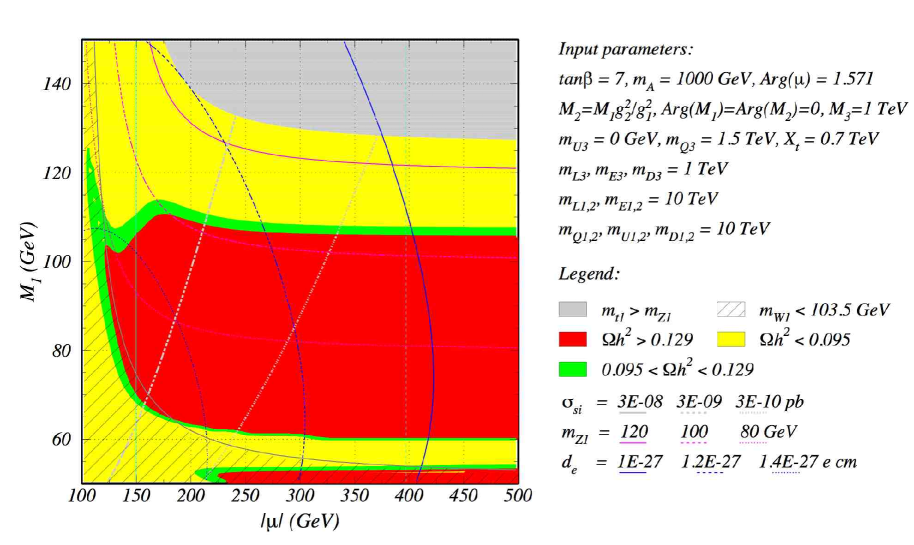
Figure 1: Neutralino relic density as a function of $M_{1}$ vs. $|\mu|$ for $m_{A}=1000$ GeV and $\arg(\mu)=\pi/2$.

The relic abundance of neutralinos is computed as described in [91], as shown in Fig. 1. This plot shows the typical dependence of the neutralino relic density on $|\mu|$ and $M_{1}$ for value of the ratio of the Higgs vacuum expectation values $\tan\beta=7$, pseudoscalar mass $m_{A}=1000$ GeV, and $\arg({\mu})=\pi/2$. The green (medium gray) bands show the region of parameter space where the neutralino relic density is consistent with the $95\%$ CL limits set by WMAP data. The regions in which the relic density is above the experimental bound and excluded by more than two standard deviations are indicated by the red (dark gray) areas. The yellow (light gray) areas show the regions of parameter space in which the neutralino relic density is less than the WMAP value. An additional source of dark matter, unrelated to the neutralino relic density, would be needed in these regions. Finally, in the (medium-light) gray region at the upper right the lightest stop becomes the LSP, while in the hatched area at the lower left corner the mass of the lightest chargino is lower than is allowed by LEP data .

The region where the relic density is too high consists of a wide band in which the lightest neutralino has mass between about 60 and 105 GeV and is predominantly bino. Above this band, the mass difference between the neutralino LSP and the light stop is less than about 20-25 GeV, and stop- neutralino coannihilation as well as stop-stop annihilation are very efficient in reducing the neutralino abundance. There is an area below the disallowed band in which the neutralino mass lies in the range 40-60 GeV, and the neutralino annihilation cross-section is enhanced by resonances from s-channel $h$ and $Z$ exchanges.

The relic density is also quite low for smaller values of $|\mu|$. In these regions, the neutralino LSP acquires a significant Higgsino component allowing it to couple more strongly to the Higgs bosons and the $Z$. This is particularly important in the region near $(|\mu|,M_{1})=(175,110)$ GeV where the neutralino mass becomes large enough that annihilation into pairs of gauge bosons through s-channel Higgs and $Z$ exchange and t-channel neutralino and chargino exchange is allowed, and is the reason for the dip in the relic density near this point. Since the corresponding couplings to the gauge bosons depend on the Higgsino content of the neutralino, these decay channels turn off as $|\mu|$ increases. For higher $M_{1}$ values, the lightest neutralino and chargino masses are also close enough that chargino-neutralino coannihilation and chargino-chargino annihilation substantially increase the effective cross section.

As suggested by universality $M_{2}=(g_{2}^{2}/g_{1}^{2})M_{1}$ is used in Fig. 1. Thus, smaller values of $M_{1}$ and $\mu$ are excluded by the lower bound on the chargino mass from LEP data , as indicated by the hatched regions in the figures. This constraint becomes much less severe for larger values of the ratio $M_{2}/M_{1}$. We also find that increasing this ratio of gaugino masses (with $M_{1}$ held fixed) has only a very small effect on the neutralino relic density.

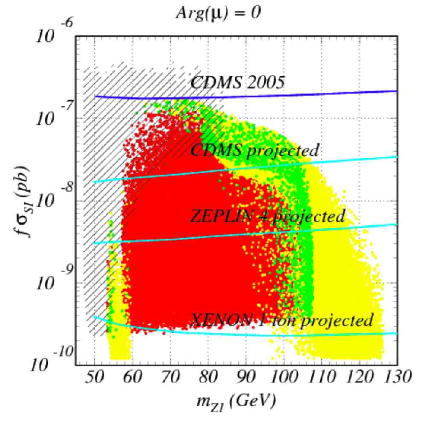
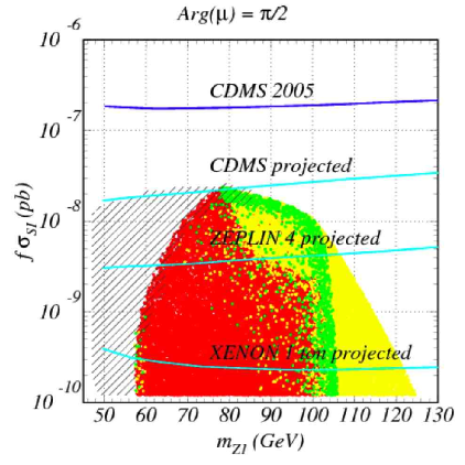
Figure 2: Spin independent neutralino-proton elastic scattering cross sections as a function of the neutralino mass for $\arg(\mu)=0$ (left) and $\arg(\mu)=\pi/2$ (right). The lower solid (cyan) lines indicate the projected sensitivity of CDMS, ZEPLIN and XENON, respectively.

The search for weakly interacting massive particles is already in progress via detection of their scattering off nuclei by measuring the nuclear recoil. Since neutralinos are non-relativistic they can be directly detected via the recoiling off a nucleus in elastic scattering. There are several existing and future experiments engaged in this search. The dependence of the neutralino-proton scattering cross section on the phase of $\mu$ has been examined as shown in Fig. 2. A random scan over the following range of MSSM parameters is conducted:

$$-(80\leavevmode\nobreak\ {\rm GeV})^{2}<m_{\tilde{U}_{3}}^{2}<0,\leavevmode\nobreak\ \leavevmode\nobreak\ \leavevmode\nobreak\ 100<|\mu|<500\leavevmode\nobreak\ {\rm GeV},\leavevmode\nobreak\ \leavevmode\nobreak\ \leavevmode\nobreak\ 50<M_{1}<150\leavevmode\nobreak\ {\rm GeV},$$

$$200<m_{A}<1000\leavevmode\nobreak\ {\rm GeV},\leavevmode\nobreak\ \leavevmode\nobreak\ \leavevmode\nobreak\ 5<\tan\beta<10.$$ (8)

The result of the scan, projected to the neutralino-proton scattering cross section versus neutralino mass plane, is shown by Fig. 2. The function $f\sigma_{SI}$ is plotted, where $f$ accounts for the diminishing flux of neutralinos with their decreasing density [151].

For models marked by yellow (light gray) dots the neutralino relic density is below the $2\sigma$ WMAP bound, while models represented by green (medium gray) dots comply with WMAP within $2\sigma$. Models that are above the WMAP value by more than $2\sigma$ are indicated by red (dark gray) dots. The hatched area is excluded by the LEP chargino mass limit of 103.5 GeV. The top solid (blue) line represents the 2005 exclusion limit by CDMS [152]. The lower solid (cyan) lines indicate the projected sensitivity of the CDMS, ZEPLIN [153] and XENON [154] experiments.

Presently, the region above the (blue) top solid line is excluded by CDMS. In the near future, for $\arg(\mu)=0$, CDMS will probe part of the region of the parameter space where the WMAP dark matter bound is satisfied. The ZEPLIN experiment will start probing the stop-neutralino coannihilation region together with the annihilation region enhanced by s-channel $A$ resonances. Finally, XENON will cover most of the relevant parameter space for small phases. Prospects for direct detection of dark matter tend to be weaker for large values of the phase of $\mu$, $\arg(\mu)\simeq\pi/2$.

Large phases, however, induce sizable corrections to the electron electric dipole moment. The EDM experiments are sensitive probes of this model [91]. Presently the experimental upper limit is

$$|d_{e}|<1.6\times 10^{-27}\;e\,cm,$$ (9)

at $90\%$ CL. One- and two loop contributions with $\mathcal{O}(1)$ phases, containing an intermediate first generation slepton or charginos and Higgs bosons, respectively, are likely larger than this limit. The one loop diagrams are suppressed by choosing high first and second generation sfermion masses in this work. The two loop corrections are suppressed by large $m_{A}$ or small $\tan\beta$. The range of $d_{e}$ values obtained in our scan are consistent with the the current electron EDM bound and EWBG. On the other hand, for $m_{A}<1000$ GeV, about an order of magnitude improvement of the electron EDM bound, $|d_{e}|<0.2\times 10^{-27}\;e\,cm$, will be sufficient to test this baryogenesis mechanism within the MSSM.

In summary, the requirement of a consistent generation of baryonic and dark matter in the MSSM leads to a well-defined scenario, where, apart from a light stop and a light Higgs boson, neutralinos and charginos are light, sizeable CP violating phases, and moderate values of $5\;\raisebox{-3.87495pt}{$\textstyle\stackrel{{\scriptstyle\textstyle<}}{{\sim}}$}\;\tan\beta\;\raisebox{-3.87495pt}{$\textstyle\stackrel{{\scriptstyle\textstyle<}}{{\sim}}$}\;10$ are expected. These properties will be tested in a complementary way by the Tevatron, the LHC and a prospective ILC, as well as through direct dark-matter detection experiments in the near future. The first tests of this scenario will probably come from electron EDM measurements, stop searches at the Tevatron and Higgs searches at the LHC within the next few years.

2.3 Baryogenesis inspired benchmark scenarios

The previous sections outlined a scenario in which the measured dark matter abundance and baryon asymmetry of the Universe can simultaneously be achieved in the context of the MSSM. For the detailed exploration of the collider phenomenology in this scenario, we follow the common strategy of selecting and analysing individual parameter space points, or benchmark points. Some of the representative parameters of the selected points, which we call Les Houches scalar top (LHS) benchmark points, are presented in Table 1. The benchmark points are defined taken into account the discussion of the the parameter values presented in the previous section.

All benchmark points are selected such that the baryon asymmetry of the Universe and the relic density of neutralinos is predicted to be close to the one measured by WMAP and pass all known low energy, collider and astronomy constraints. The most important of these are the SUSY particle masses, the electron EDM, $B(b\to s\gamma)$, and direct WIMP detection. A crucial constraint is the LEP 2 Higgs boson mass limit of $m_{h}>114.4$ GeV. In the calculations of the supersymmetric spectrum and the baryon asymmetry, tree level relations are used except for the Higgs mass, which is calculated at the one loop level. In the parameter region of interest, the one loop calculation results in about 6-8 GeV lower lightest Higgs mass than the two loop one [155, 156]. Thus, if the soft supersymmetric parameters defining the benchmark points are used in a two loop calculation, the resulting lightest Higgs mass is found to be inconsistent with LEP 2. A two loop level consistency with the LEP 2 limit can be achieved only when a baryon asymmetry calculation becomes available using two loop Higgs boson masses.

The main difference between the benchmark points lies in the mechanism that ensures that the neutralino relic density also complies with WMAP. Keeping the unification motivated ratio of the gaugino mass parameters $M_{2}/M_{1}$ close to 2 (together with the baryogenesis required $100\;\raisebox{-3.87495pt}{$\textstyle\stackrel{{\scriptstyle\textstyle<}}{{\sim}}$}\;|\mu|\;\raisebox{-3.87495pt}{$\textstyle\stackrel{{\scriptstyle\textstyle<}}{{\sim}}$}\;500$ GeV) induces a lightest neutralino with mostly bino admixture. A bino typically overcloses the Universe, unless there is a special situation that circumvents this. For example, as in the supergravity motivated minimal scenario mSUGRA, neutralinos can coannihilate with sfermions, resonant annihilate via Higgs bosons, or acquire a sizable Higgsino admixture in special regions of the parameter space. This lowers the neutralino density to a level that is consistent with the observations.

	LHS-1	LHS-2	LHS-3	LHS-4
$m_{{\tilde{Q},\tilde{U},\tilde{D}}_{1,2}}$	10000	10000	10000	4000
$m_{{\tilde{Q}}_{3}}$	1500	1500	1500	4200
$m_{{\tilde{U}}_{3}}^{2}$	0	0	0	$-99^{2}$
$m_{{\tilde{D}}_{3}}$	1000	1000	1000	4000
$m_{{\tilde{L}}_{1,2}}$	10000	10000	10000	2000
$m_{{\tilde{L}}_{3}}$	1000	1000	1000	2000
$m_{{\tilde{E}}_{1,2}}$	10000	10000	10000	200
$m_{{\tilde{E}}_{3}}$	1000	1000	1000	200
$A_{b}$	0	0	0	0
$A_{t}$	$-650\times e^{-i\pi/2}$	$-643\times e^{-i\pi/2}$	$-676\times e^{-i\pi/2}$	$-$1050
$A_{e,\mu,\tau}$	0	0	0	5000$\times e^{i\pi/2}$
$M_{1}$	110	60	110	112.6
$M_{2}$	220	121	220	225.2
$|\mu|$	350	400	165	320
$\arg(\mu)$	$\pi/2$	$\pi/2$	$\pi/2$	0.2
$\tan(\beta)$	7	7	7	5
$m_{A}$	1000	1000	1000	800
$m_{{\tilde{t}}_{1}}$	137	137	137	123
$m_{{\tilde{t}}_{2}}$	1510	1510	1510	4203
$m_{{\tilde{e}}_{1}}$	9960	9960	9960	204
$m_{{\tilde{e}}_{2}}$	10013	10013	10013	2000
$m_{{\tilde{\chi}}^{0}_{1}}$	106	58.1	89.2	107
$m_{{\tilde{\chi}}^{0}_{2}}$	199	112	145	196
$m_{{\tilde{\chi}}^{+}_{1}}$	197	111	129	194
$m_{{\tilde{\chi}}^{+}_{2}}$	381	419	268	358
$m_{h}$	116	116	116	117
$Br({\tilde{t}}_{1}\to{\tilde{\chi}}^{0}_{1}c)$	1	0	0	1
$Br({\tilde{t}}_{1}\to{\tilde{\chi}}^{\pm}_{1}b)$	0	1	1	0
$\Omega_{{\tilde{\chi}}^{0}_{1}}h^{2}$	0.10	0.11	0.11	0.11

Table 1: Les Houches scalar top (LHS) benchmark points motivated by baryogenesis and neutralino dark matter. Parameters with mass dimensions are given in GeV units. The detailed definition of the LHS benchmarks, in SLHA format [92], can be downloaded from http://www.hep.anl.gov/balazs/Physics/LHS/.

Benchmark point LHS-1 features strong stop-neutralino coannihilation which lowers the relic density of neutralinos close to the WMAP central value. Sizable coannihilation only occurs when the mass difference between the neutralino and stop is small (less than about 30-40%). It is shown in the following sections that a small neutralino-stop mass gap poses a challenge for the Tevatron and the LHC while the ILC can cover this region efficiently.

At benchmark LHS-2 resonant annihilation of neutralinos via s-channel Higgs resonances lowers the neutralino abundance to the measured level. In this case, the neutralino mass must be very close to half of the lightest Higss boson mass. This point features a stop that, given enough luminosity, can be discovered at the Tevatron due to the large difference between the stop and the neutralino masses. Even the heavier stop can possibly be produced at the LHC together with the third generation sleptons. On the other hand, since the resonance feature, the lightest Higgs boson can decay into neutralinos, which reduces its visible width, and can make its discovery more challenging.

Point LHS-3 satisfies the WMAP relic density constraint partly because the lightest neutralino acquires some wino admixture and because it is coannihilating with the lightest stop and chargino. The multiple effects lowering the relic density allow for a little larger neutralino-stop mass gap than in LHS-1. This point has a neutralino-stop mass gap that makes it detectable at the Tevatron and the LHC.

LHS-4, a variation of LHS-1, is defined in detail in Ref. [157]. Here the small neutralino-stop mass difference makes the light stop inaccessible at the Tevatron and the LHC. On the other hand, the ILC could measure the parameters with precision. The discovery potential of this point is discussed in detail in Section 6

In summary, the four benchmark points offer various challenges for the three colliders. The Tevatron could resolve the stop quark in points LHS-2 and LHS-3, where the ${\tilde{t}}_{1}$ decays into ${\tilde{\chi}}_{1}^{\pm}b$, but not in LHS-1 and LHS-4, where it decays into ${\tilde{\chi}}_{1}^{0}c$ with a small phase space. The LHC on the other hand may explore LHS-1 via the method described in 3, and LHS-2 as described in 4. In principle these methods are also applicable for LHS-4 and LHS-3; the small mass differences at these points, however, make the analysis much more difficult. In LHS-1, LHS-2 and LHS-3 the LHC can pair produce the heavier stop, which is needed to pin down the stop sector so crucial for baryogenesis. At the ILC, one can perform precision measurements of the light stop as shown in section 6. Moreover, the -ino sector including the important phase(s) can be measured precisely (see [40] and references therein).

3 SAME-SIGN TOPS AS SIGNATURE OF LIGHT STOPS AT THE LHC

If the lighter of the two stops, $\tilde{t}_{1}$, has a mass $m_{\tilde{t}_{1}}\;\raisebox{-3.87495pt}{$\textstyle\stackrel{{\scriptstyle\textstyle<}}{{\sim}}$}\;m_{t}$ as motivated by baryogenesis [127, 158, 159, 160], gluino decays into stops and tops will have a large branching ratio. Since gluinos are Majorana particles, they do not distinguish between $t\tilde{t}_{1}^{*}$ and $\bar{t}\tilde{t}_{1}$ combinations. Pair-produced gluinos therefore give

$$\tilde{g}\tilde{g}\to t\bar{t}\,\tilde{t}_{1}\tilde{t}_{1}^{*},\;tt\,\tilde{t}_{1}^{*}\tilde{t}_{1}^{*},\;\bar{t}\bar{t}\,\tilde{t}_{1}\tilde{t}_{1}$$ (10)

and hence same-sign top quarks in half of the gluino-to-stop decays. For $m_{\tilde{t}_{1}}-m_{\tilde{\chi}^{0}_{1}}<m_{W}$, the $\tilde{t}_{1}$ further decays into $c\tilde{\chi}^{0}_{1}$. If, in addition, the $W$ stemming from $t\to bW$ decays leptonically, a signature of two $b$ jets plus two same-sign leptons plus jets plus missing transverse energy is expected:

$$pp\to\tilde{g}\tilde{g}\to bb\,l^{+}l^{+}\>({\rm or}\>\bar{b}\bar{b}\,l^{-}l^{-})+{\rm jets\>}+\not\!\!E_{T}\,.$$ (11)

This is a quite distinct peculiar signature, which will serve to remove most backgrounds, both from SM and Supersymmetry. Even though $\tilde{t}_{1}$ pair production has the dominant cross section, it leads to a signature of two $c$-jets and missing transverse energy, which is of very limited use. Thus the same-sign top signature is of particular interest in our scenario. In this contribution, we lay out the basics of the analysis; for a detailed description see [161].

To investigate the use of our signature, Eq. (11), for discovering a light $\tilde{t}_{1}$ at the LHC we define a MSSM benchmark point ‘LST-1’ with $m_{\tilde{g}}=660$ GeV, $m_{\tilde{t}_{1}}=150$ GeV and $m_{\tilde{\chi}^{0}_{1}}=105$ GeV. The other squarks (in particular the sbottoms) are taken to be heavier than the gluinos. This considerably suppresses the SUSY background, and gluinos decay to about 100% into $t\tilde{t}_{1}$. For the neutralino to have a relic density within the WMAP bound, we choose $m_{A}=250$ GeV. The MSSM parameters of LST-1 and the corresponding masses, calculated with SuSpect 2.3 [62], are given in Tables 2 and 3 (as for the LHS points, the SUSY-breaking parameters are taken to be onshell.). The relic density computed with micrOMEGAs [5, 6] is $\Omega h^{2}=0.105$.

$M_{1}$	$M_{2}$	$M_{3}$	$\mu$	$\tan(\beta)$
110	220	660	300	7
$m_{A}$	$A_{t}$	$A_{b}$	$A_{\tau}$
250	$-670$	$-500$	100
$m_{\tilde{L}_{1,2}}$	$m_{\tilde{L}_{3}}$	$m_{\tilde{Q}_{1,2}}$	$m_{\tilde{Q}_{3}}$
250	250	1000	1000
$m_{\tilde{E}_{1,2}}$	$m_{\tilde{E}_{3}}$	$m_{\tilde{U}_{1,2}}$	$m_{\tilde{D}_{1,2}}$	$m_{\tilde{U}_{3}}$	$m_{\tilde{D}_{3}}$
250	250	1000	1000	100	1000
$\alpha_{\mathrm{e}m}^{-1}(m_{Z})^{\overline{\mathrm{MS}}}$	$G_{F}$	$\alpha_{s}(m_{Z})^{\overline{\mathrm{MS}}}$	$m_{Z}$	$m_{b}(m_{b})^{\overline{\mathrm{MS}}}$	$m_{t}$	$m_{\tau}$
127.91	$1.1664\times 10^{-5}$	0.11720	91.187	4.2300	175.0	1.7770

Table 2: Input parameters for the LST-1 scenario [masses in GeV]. Unless stated otherwise, the SM masses are pole masses. The SUSY-breaking parameters are taken to be onshell.

$\tilde{d}_{L}$	$\tilde{u}_{L}$	$\tilde{b}_{1}$	$\tilde{t}_{1}$	$\tilde{e}_{L}$	$\tilde{\tau}_{1}$	$\tilde{\nu}_{e}$	$\tilde{\nu}_{\tau}$
1001.69	998.60	997.43	149.63	254.35	247.00	241.90	241.90
$\tilde{d}_{R}$	$\tilde{u}_{R}$	$\tilde{b}_{2}$	$\tilde{t}_{2}$	$\tilde{e}_{R}$	$\tilde{\tau}_{2}$
1000.30	999.40	1004.56	1019.26	253.55	260.73
$\tilde{g}$	$\tilde{\chi}^{0}_{1}$	$\tilde{\chi}^{0}_{2}$	$\tilde{\chi}^{0}_{3}$	$\tilde{\chi}^{0}_{4}$	$\tilde{\chi}^{\pm}_{1}$	$\tilde{\chi}^{\pm}_{2}$
660.00	104.81	190.45	306.06	340.80	188.64	340.09
$h$	$H$	$A$	$H^{\pm}$
118.05	251.52	250.00	262.45

Table 3: SUSY mass spectrum [in GeV] for the LST-1 scenario. For the squarks and sleptons, the first two generations have identical masses.

3.1 Event generation

We have generated SUSY events and $t\bar{t}$ background equivalent to $30\leavevmode\nobreak\ \mathrm{fb}^{-1}$ of integrated luminosity with PYTHIA 6.321 [17] and CTEQ 5L parton distribution functions [47]. This corresponds to about three years of data-taking at the LHC at low luminosity. The cross sections for the Supersymmetry processes at NLO are given in Table 4. We have also generated additional SM background in five logarithmic $p_{T}$ bins from $p_{T}=50$ GeV to $4000$ GeV, consisting of $5\times 10^{4}$ of $W$+jet, $Z$+jet, and $WW/WZ/ZZ$ production events and $1.5\times 10^{5}$ QCD $2\rightarrow 2$ events per bin.

	$\sigma(\tilde{t}_{1}\tilde{t}_{1})$	$\sigma(\tilde{g}\tilde{g})$	$\sigma(\tilde{g}\tilde{q})$	$\sigma(\tilde{\chi}^{0}_{2}\tilde{\chi}^{\pm}_{1})$	$\sigma(\tilde{\chi}^{\pm}_{1}\tilde{\chi}^{\mp}_{1})$	$\sigma(\tilde{q}\tilde{q})$	$\sigma(\tilde{q}\tilde{q}^{*})$	$\sigma(\tilde{\chi}^{\pm}_{1}\tilde{g})$	$\sigma(t\bar{t})$
LST-1	$280$	$5.39$	$4.98$	$1.48$	$0.774$	$0.666$	$0.281$	$0.0894$	$737$

Table 4: Cross sections (in pb) at NLO for the most important Supersymmetric processes for LST-1 parameters, computed with Prospino2 [162] at $\sqrt{s}=14$ TeV. For comparison, we also give the $t\bar{t}$ NLO cross section taken from [15].

Detector simulation are performed with the generic LHC detector simulation AcerDET 1.0 [163]. This expresses identification and isolation of leptons and jets in terms of detector coordinates by azimuthal angle $\phi$, pseudo-rapidity $\eta$ and cone size $\Delta R=\sqrt{(\Delta\phi)^{2}+(\Delta\eta)^{2}}$. We identify a lepton if $p_{T}>5$ (6) GeV and $|\eta|<2.5$ for electrons (muons). A lepton is isolated if it is a distance $\Delta R>0.4$ from other leptons and jets, and the transverse energy deposited in a cone $\Delta R=0.2$ around the lepton is less than $10$ GeV. Jets are reconstructed from clusters by a cone-based algorithm and are accepted if the jet has $p_{T}>15$ GeV in a cone $\Delta R=0.4$. The jets are recalibrated using a flavour-independent parametrization, optimized to give a scale for the dijet decay of a light Higgs. The $b$-tagging efficiency and light jet rejection are set according to the $p_{T}$ parametrization for a low luminosity environment, given in [164].

3.2 Signal isolation

The following cuts are applied:

• two same-sign leptons ($e$ or $\mu$) with $p^{\mathrm{lep}}_{T}>20$ GeV.

• at least four jets with $p^{\mathrm{jet}}_{T}>50$ GeV, of which two are $b$-tagged.

• $\not{\!\!E}_{T}>100$ GeV.

• The top quark content in the events is explored by demanding two combinations of the two hardest leptons and $b$-jets that give invariant masses $m_{bl}<160$ GeV, which is consistent with a top quark.

The effects of these cuts are shown in Table 5 where “2lep 4jet” is after detector simulation and cuts on two reconstructed and isolated leptons and four reconstructed jets; “2b” is the number of events left after the $b$-jet cut, assuming a $b$-tagging efficiency of 43%; “$\not{\!\!E}_{T}$” is the cut on missing transverse energy and “SS” the requirement of two same-sign leptons. These cuts constitute the signature of Eq. (11). The same-sign cut is of central importance in removing the SM background, which at this point consists only of $t\bar{t}$ events. The cuts on transverse momentum and top content “2$t$” are used to further reduce the background. We find that the gluino pair production, with leptonic top decay, is easily separated from both SM and SUSY backgrounds.

Cut	2lep 4jet	$p_{T}^{\mathrm{lep}}$	$p_{T}^{\mathrm{jet}}$	2b	$\not\!\!E_{T}$	2$t$	SS
Signal
$\tilde{g}\tilde{g}\to t\bar{t}\,\tilde{t}_{1}\tilde{t}_{1}^{*},\;tt\,\tilde{t}_{1}^{*}\tilde{t}_{1}^{*},\;\bar{t}\bar{t}\,\tilde{t}_{1}\tilde{t}_{1}$	10839	6317	4158	960	806	628	330
Background
SUSY	1406	778	236	40	33	16	5
SM	25.3M	1.3M	35977	4809	1787	1653	12

Table 5: Number of events after cumulative cuts for $30\leavevmode\nobreak\ \mathrm{fb}^{-1}$ of integrated luminosity.

We have assumed vanishing flavour-changing neutral currents (FCNCs), so that the anomalous couplings in $tgc$ and $tgu$ vertices are effectively zero, i.e.  there is no significant same-sign top production by FCNCs. To investigate other possible backgrounds we have used MadGraph II with the MadEvent event generator [165, 166]. The search has been limited to parton level, as we find no processes that can contribute after placing appropriate cuts. We have investigated the SM processes that can mimic a same-sign top pair by mis-tagging of jets or the production of one or more additional leptons, as well as inclusive production of same-sign top pairs. In particular we have investigated the diffractive scattering $qq\to W^{\pm}q^{\prime}W^{\pm}q^{\prime}$ and the production of a top pair from gluon radiation in single $W$ production $qq^{\prime}\to t\bar{t}W^{\pm}$. We have also checked the production of $t\bar{t}l^{+}l^{-}$, $t\bar{t}t\bar{t}$, $t\bar{t}t\bar{b}$, $t\bar{t}b\bar{t}$, $tW^{-}tW^{-}$, $\bar{t}W^{+}\bar{t}W^{+}$ and $W^{\pm}W^{\pm}b\bar{b}jj$.Cuts on leptons and quarks have been placed as given above, and two lepton-quark pairs are required to be consistent with top decays. We also require neutrinos from the $W$ decays to give the needed missing energy. After these cuts and detector geometry cuts of $\Delta R>0.4$ and $|\eta|<2.5$ for all leptons and quarks, we find the cross sections of these processes to be too small, by at least an order of magnitude, to make a contribution at the integrated luminosity considered.

3.3 Mass determination

Having isolated the signal, it will be important to measure the properties of the sparticles to confirm that the decay indeed involves a light scalar top. Since the neutralino and the neutrino in the top decay represent missing energy and momentum, reconstruction of a mass peak is impossible. The well studied alternative to this, see e.g. [167, 168, 169, 170, 171], is to use the invariant-mass distributions of the SM decay products. Their endpoints can be given in terms of the SUSY masses, and these equations can then in principle be solved to give the masses.

In this scenario there are two main difficulties. First, there are four possible endpoints: $m_{bl}^{\max}$, $m_{bc}^{\max}$, $m_{lc}^{\max}$ and $m_{blc}^{\max}$, of which the first simply gives a relationship between the masses of the $W$ and the top, and the second and third are linearly dependent, so that we are left with three unknown masses and only two equations. Second, because of the information lost with the escaping neutrino, the distributions of interest all fall very gradually to zero. Determining exact endpoints in the presence of background, while taking into account smearing from the detector, effects of particle widths, etc., will be very difficult. The shape of the invariant-mass distributions are shown, for some arbitrary normalization, in Fig. 3.

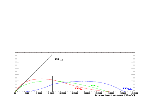
Figure 3: Invariant-mass distributions for LST-1 at generator level. These distributions only take into account the kinematics of the decay.

We have attacked the second problem by extending the endpoint method and deriving the complete shapes of the invariant-mass distributions for $m_{bc}$ and $m_{lc}$. The resulting expressions, and their derivation, are too extensive to be included here, but can be found in [161]. Fitting to the whole distribution of invariant mass greatly reduces the uncertainty involved in endpoint determination, and has the possibility of giving additional information on the masses. One could also imagine extending this method to include spin effects in the distribution, to get a handle on the spins of the SUSY particles involved .

In fitting the $m_{bc}$ and $m_{lc}$ distributions, we start from the isolated gluino pair production events of Section 3.2. However, in some of these events one or both of the $W$ decay to a tau lepton, which in turn decays leptonically; these are an additional, irreducible background to the signal distributions. The $b$-jets and leptons are paired through the cut on two top-quark candidates. A comparison with Monte Carlo information from the event generation shows that this works well in picking the right pairs. The issue remains to identify the $c$-quark-initiated jets and to assign these them to the correct $b$-jet and lepton pair. The precision of this endpoint determination is limited by systematical uncertainties.

Different strategies can be used for picking the $c$-jets. Because of the strong correlation between the tagging of $b$- and $c$-jets, one could use an inclusive $b/c$-jet tagging where the two types of jets would be separated by their $b$-tagging likelihoods, and the requirement of top candidates in the event. A thorough investigation of this strategy will require a full simulation study, using realistic $b$-tagging routines. The strategy that we follow here is, instead, to accept a low $b$-tagging efficiency to pick two $b$-jets and reject most $c$-jets. The likelihoods in the $b$-tagging routine could then help to pick the correct $c$-jets from the remaining jets. In this fast simulation study we are restricted to a simple statistical model of the efficiency of making this identification and we assume a $20\%$ probability of identifying a $c$-jet directly from the $b$-tagging likelihood. For events where we have missed one or both of the $c$-jets, they are selected as the two hardest remaining jets with $p_{T}^{\mathrm{jet}}<100$ GeV. This upper bound on transverse momentum is applied because the stop is expected to be relatively light if our signal exists, and it avoids picking jets from the decay of heavy squarks. The $c$-jet candidates are paired to the top candidates by their angular separation in the lab frame, and by requiring consistency with the endpoints of the two invariant-mass distributions we are not looking at. For example, to construct the $m_{bc}$ distribution, we demand consistency with the endpoints $m_{lc}^{\max}$ and $m_{blc}^{\max}$ . Events with no consistent combinations of $c$-jets and top-quark candidates are rejected.

The fit functions for $m_{bc}$ and $m_{lc}$ can in principle be used to determine both of the two linearly independent parameters

$$(m_{bc}^{\max})^{2}=\frac{(m_{t}^{2}-m_{W}^{2})(m_{\tilde{t}_{1}}^{2}-m_{\tilde{\chi}_{1}^{0}}^{2})(m_{1}^{2}+m_{2}^{2})}{2m_{t}^{2}m_{\tilde{t}_{1}}^{2}}\quad\textrm{and}\quad a=\frac{m_{2}^{2}}{m_{1}^{2}},$$ (12)

where

$$m_{1}^{2}=m_{\tilde{g}}^{2}-m_{t}^{2}-m_{\tilde{t}_{1}}^{2}\quad\textrm{and}\quad m_{2}^{4}=m_{1}^{4}-4m_{t}^{2}m_{\tilde{t}_{1}}^{2}.$$ (13)

We typically have $m_{t}m_{\tilde{t}_{1}}\ll m_{\tilde{g}}^{2}$ for light stops, so that $a\approx 1$. In our model the nominal value is $a=0.991$. The distributions are sensitive to such values of $a$ only at very low invariant masses. Because of the low number of events, no sensible value can be determined from a fit; we therefore set $a=1$. The fit quality and value of $m_{bc}^{\max}$ is found to be insensitive to the choice of $a$ for $a\;\raisebox{-3.87495pt}{$\textstyle\stackrel{{\scriptstyle\textstyle>}}{{\sim}}$}\;0.980$.

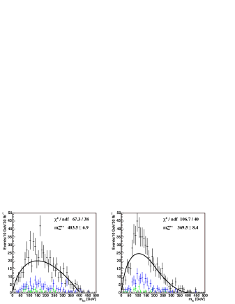
Figure 4: Invariant-mass distributions with $20\%$ $c$-tagging efficiency after $b$-tagging. The left plot shows $m_{bc}$ (black), the right plot shows $m_{lc}$ together with a fit of the calculated distribution. Also shown are the contributions from the SM background (green) and the SUSY background (blue). The SUSY background consists mostly of events with one or more taus.

The results of the fits to $m_{bc}^{\max}$ are shown in Fig. 4. The combined result of the two distributions is $m_{bc}^{\max}=389.8\pm 5.3$ GeV, to be compared with the nominal value of $391.1$ GeV. The somewhat large $\chi^{2}$ values of the fits indicate that there are some significant systematical errors. However, if this is compared to the same fit with no $c$-tagging, we find large improvements in both fit quality and distance from the nominal value. The analysis can be optimized using more detailed information from the $b$-quark tagging.

In summary, we have investigated a baryogenesis-motivated scenario of a light stop ($m_{\tilde{t}_{1}}\;\raisebox{-3.87495pt}{$\textstyle\stackrel{{\scriptstyle\textstyle<}}{{\sim}}$}\;m_{t}$), with $\tilde{t}_{1}\to c\tilde{\chi}^{0}_{1}$ as the dominant decay mode. In this scenario, pair production of $\tilde{t}_{1}$ leads to a signature of two jets and missing transverse energy, which will be difficult to be used for the discovery of $\tilde{t}_{1}$ at the LHC. We have hence proposed a method using stops stemming from gluino decays: in gluino pair production, the Majorana nature of the gluino leads to a peculiar signature of same-sign top quarks in half of the gluino-to-stop decays. For the case in which all other squarks are heavier than the gluino, we have shown that the resulting signature of $2b$’s + 2 same-sign leptons + jets $+\not{\!\!E}_{T}$ can easily be extracted from the background and serve as a discovery channel for a light $\tilde{t}_{1}$. We have also demonstrated the measurement of a relationship between the gluino, stop and LSP masses. Taken together with a determination of other invariant-mass endpoints, and a measurement of the SUSY mass scale from the effective mass scale of events, this may be sufficient to approximately determine the masses of the SUSY particles involved, in particular the light stop. Last but not least we have checked that the same-sign top signal remains robust for higher gluino masses, for the case $m_{\tilde{b}}<m_{\tilde{g}}$, as well as in the stop co-annihilation region with a small mass difference between the $\tilde{t}_{1}$ and the LSP. See [161] for more details.

4 DETECTION OF A LIGHT STOP SQUARK WITH THE ATLAS DETECTOR AT THE LHC

It has been recently pointed out that SUSY models with a very light stop squark, lighter than the top quark, not excluded by existing accelerator searches, can have an important impact for cosmology [127, 160, 91].

Little work had been devoted to date to explore the potential of the LHC experiments for the discovery of light stop squarks. In the framework of the 2005 Les Houches Workshop it was therefore decided to address this issue by studying the detectability of the stop at the LHC in two benchmark models. For both of these models the stop quark has a mass of 137 GeV, and for the first, easier, model the two-body decay of the stop squark into a chargino and a $b$ quark is open. For the second model the chargino is heavier than the stop, which has therefore to decay either in the 4-body mode $W^{*}b{\tilde{\chi}_{1}^{0}}$ or through a loop to $c{\tilde{\chi}_{1}^{0}}$.

An exploratory study is presented of the first of the two models, where we address in detail the ability of separating the stop signal from the dominant SM backgrounds. The parameters of the examined model correspond to that of the LHS-2 benchmark point.

4.1 Simulation parameters

For the model under study all the masses of the first two generation squarks and sleptons are set at 10 TeV, and the gaugino masses are related by the usual gaugino mass relation $M_{1}:M_{2}=\alpha_{1}:\alpha_{2}$. The remaining parameters are thus defined:

$$M_{1}=60.5\leavevmode\nobreak\ {\rm GeV}\;\;\;\mu=400\leavevmode\nobreak\ {\rm GeV}\;\;\;\tan\beta=7\;\;\;M_{3}=950\leavevmode\nobreak\ {\rm GeV}$$

$$m(Q_{3})=1500\leavevmode\nobreak\ {\rm GeV}\;\;\;m({\tilde{t}}_{R})=0\leavevmode\nobreak\ {\rm GeV}\;\;\;m({\tilde{b}}_{R})=1000\leavevmode\nobreak\ {\rm GeV}\;\;\;A_{t}=-642.8\leavevmode\nobreak\ {\rm GeV}$$

The resulting relevant masses are $m({\tilde{t}}_{1})=137$ GeV, $m({\tilde{\chi}}^{\pm}_{1})=111$ GeV, $m({\tilde{\chi}_{1}^{0}})=$58 GeV. The ${\tilde{t}}_{1}$ decays with 100% branching ratio into ${\tilde{\chi}}^{\pm}_{1}b$, and ${\tilde{\chi}}^{\pm}_{1}$ decays with 100% branching ratio into an off-shell $W$ and ${\tilde{\chi}}^{0}_{1}$. The final state signature is therefore similar to the one for $t\bar{t}$ production: 2 $b$-jets, $E_{T}^{miss}$ and either 2 leptons ($e,\mu$) (4.8% branching ratio) or 1 lepton and 2 light jets (29% BR).

The signal cross-section, calculated with the CTEQ5L structure functions is 280 pb at leading order. The NLO result, calculated with the PROSPINO [173] program is 412 pb. This corresponds to approximately half of the cross-section for top quark production.
For the signal a softer kinematics of the visible decay products is expected, compared to the top, since the mass difference between the stop and the invisible ${\tilde{\chi}_{1}^{0}}$ at the end of the decay chain is about 80 GeV. We analyze here the semi-leptonic channel, where only one of the two ${\tilde{t}}_{1}$ legs has a lepton in the final state. We apply the standard cuts for the search of the semileptonic top channel as applied in [174], but with softer requirements on the kinematics:

• one and only one isolated lepton ($e$, $\mu$), $p_{T}^{l}>20$ GeV.

• $E_{T}^{miss}>20$ GeV.

• at least four jets with $P_{T}(J_{1},J_{2})>35$ GeV and $P_{T}(J_{3},J_{4})>25$ GeV.

• exactly two jets in the events must be tagged as $b$-jets. They both must have $p_{T}>20$ GeV. The standard ATLAS b-tagging efficiency of 60% for a rejection factor of 100 on light jets is assumed.

A total of 600k SUSY events were generated using HERWIG 6.5 [11, 12], and 1.2M $t\bar{t}$ events using PYTHIA 6.2 [175]. This corresponds to a statistics of about 2.5 fb^-1 for the LO cross-sections and about $1.8$ fb^-1 for the NLO cross-sections. The only additional background considered for this exploratory study was the associated production of a W boson with two $b$ jets and two non-$b$ jets. This is the dominant background for top searches at the LHC. We generated this process with ALPGEN [176]. The cross-section for the kinematic cuts applied at generation is 34 pb for $W$ decaying to both $e$ and $\mu$. A total of about $60000$ events were generated for this background. For this exploratory study we just generated the process $Wbbjj$, which should allow us to have an idea whether this background will strongly affect the analysis. A more accurate estimate of this background should be performed by generating all of the $Wbb$+(1,..n) jets with the appropriate matching to the parton shower. The generated events are then passed through ATLFAST, a parametrized simulation of the ATLAS detector [18].

4.2 Analysis

After the described selection cuts the efficiency for the $t\bar{t}$ background is 3.3%, for $Wbbjj$ 3.1%, and for the signal 0.47%, yielding a background which is about 15 times larger than the signal.
An improvement of the signal/background ratio can be obtained by requiring on the minimum invariant mass of all the non-b jets $p_{T}>25$ GeV in the event. The distribution for signal and background is shown in Fig. 5.

 

Figure 5: Minimum invariant mass distributions (in GeV) of two non-b jets for signal (left) and background (right).

A clear peak for the W mass is visible for the top background, whereas the invariant mass for the signal should be smaller than about 54 GeV, which is the mass difference between the ${\tilde{\chi}}^{\pm}$ and the ${\tilde{\chi}}^{0}_{1}$. In this analysis we are searching for the possible evidence of a light stop, for which the decay through a resonant $W$ is kinematically not allowed. It is therefore possible to significantly improve the signal/background ratio by selecting the events where $m_{jj}<60$ GeV. The signal/background ratio improves to 1/10, with a loss of a bit more than half the signal. This cut could bias the kinematic distribution for the signal, which has a priori an unknown kinematics. We have therefore repeated the analysis for a cut at 70 GeV as a systematic check, obtaining equivalent results. Figure 6 shows the $m(bjj)_{\rm min}$ distribution after this cut, i.e. the invariant mass for the combination of a b-tagged jet and the two non-b jets yielding the minimum invariant mass. If the selected jets result from the decay of the stop, the invariant mass should have an end point at about 79 GeV, whereas the corresponding end-point should be at 175 GeV for the top background. The presence of the stop signal is therefore visible as a shoulder in the distribution compared to the pure top contribution. A significant contribution from $Wbb$ is present, without a particular structure.

 

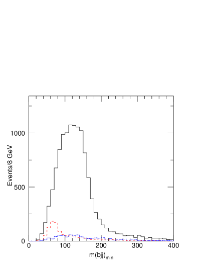
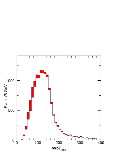
Figure 6: Left: minimum $bjj$ invariant mass distributions (in GeV) for top background (full black line), $Wbb$ background (dot-dashed blue line), signal (dashed red line). Right: same distribution, showing the signal contribution (gray) summed to the background.

Likewise, the variable $m(bl)_{min}$ has an end point at about 66 GeV for the signal and at 175 GeV for the top background, as shown in Fig. 7. The same shoulder structure is observable. We need therefore to predict precisely the shape of the distributions for the top background in order to subtract it from the experimental distributions and extract the signal distributions.

 

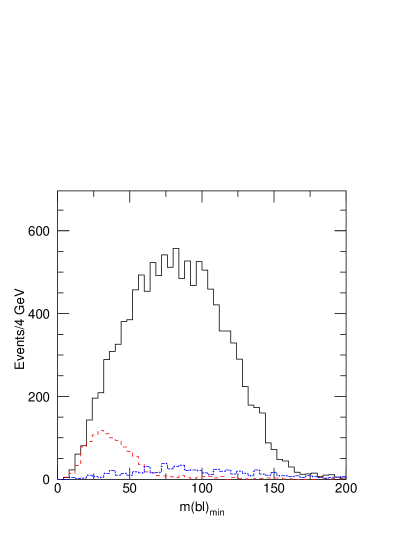
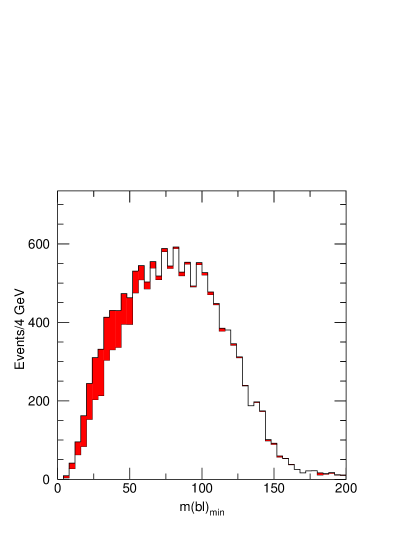
Figure 7: Left: minimum $bl$ invariant mass distributions (in GeV) for top background (full black line), $Wbb$ background (dot-dashed blue line), signal (dashed red line). Right: same distribution, showing the signal contribution (gray) summed to the background.

The top background distributions can be estimated from the data themselves by exploiting the fact that we select events where one of the $W$ from the top decays decays into two jets and the other decays into lepton neutrino. One can therefore select two pure top samples, with minimal contribution from non-top events by applying separately hard cuts on each of the two legs.

• Top sample 1: the best reconstructed $bl\nu$ invariant mass is within 15 GeV of 175 GeV, and $m(bl)_{min}>60$ GeV in order to minimize the contribution from the stop signal. The neutrino longitudinal momentum is calculated by applying the $W$ mass constraint.

• Top sample 2: the best reconstructed $bjj$ mass is within 10 GeV of 175 GeV.

 

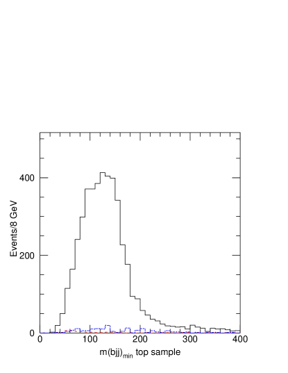
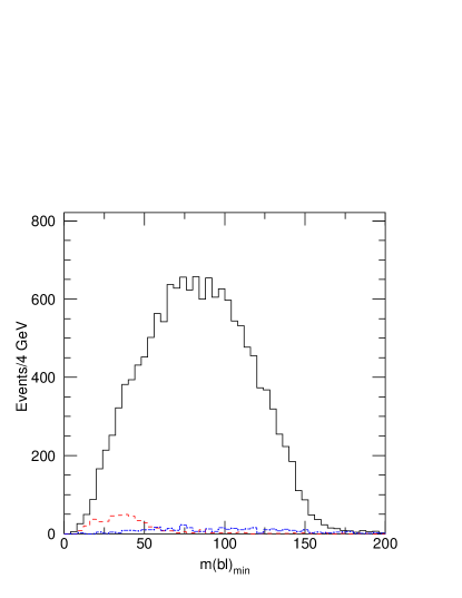
Figure 8: Left: minimum $bjj$ invariant mass distribution (in GeV) for top background (full black line), $Wbb$ background (dot-dashed blue line), signal (dashed red line) for top sample 1. Right: minimum $bl$ invariant mass distribution (in GeV) for top background (full black line), $Wbb$ background (dot-dashed blue line), signal (dashed red line) for top sample 2.

The distributions of $m(bjj)_{\rm min}$ ($m(bl)_{min}$) for signal and background are shown in Fig. 8 left (right plot) for top sample 1 (top sample 2), respectively. Only a small amount of signal and $Wbb$ background is present in the top samples, and in particular the signal is reduced essentially to zero for masses above 80 GeV.

We assume that we will be able to predict the $Wbb$ background through a combination of Monte Carlo and the study of $Zbb$ production in the data, and we subtract this background both from the observed distributions and from the top samples. More work is required to assess the uncertainty on this subtraction. Given the fact that this background is smaller than the signal, and it has a significantly different kinematic distribution, we expect that a 10-20% uncertainty will not affect the conclusions of the present analysis.

 

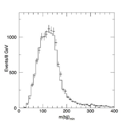
Figure 9: Left: minimum $bjj$ invariant mass distribution (in GeV) for background (full line) and rescaled top sample 1 (points with errors). Right: minimum $bl$ invariant mass distribution (in GeV) for background (full line) and rescaled top sample 2 (points with errors).

For top sample 1, the top selection is performed by applying severe cuts on the lepton leg, it can therefore be expected that the minimum $bjj$ invariant mass distribution, which is built from jets from the decay of the hadronic side be essentially unaffected by the top selection cuts. This is shown in the left plot of Fig. 9 where the minimum $bjj$ invariant mass distribution, after subtraction of the residual $Wbb$ background is compared to the distribution for a pure top sample. The top sample 1 is rescaled in such a way that the integral of the two distributions is the same in the higher mass part of the spectrum, where essentially no signal is expected. The agreement is quite good, clearly good enough to allow the extraction of the stop signal.

A similar result is observed for the minimum $bl$ invariant mass and top sample 2, as shown on the right plot of Fig. 9.

 

Figure 10: Left: minimum $bjj$ invariant mass distribution (in GeV) after the subtraction procedure (points with errors) superimposed to the original signal distribution (full line). Right: minimum $bl$ invariant mass distribution (in GeV) after the subtraction procedure (points with errors) superimposed to the original signal distribution (full line).

The rescaled $m(bjj)_{\rm min}$ ($m(bl)_{min}$) for top sample 1 (2) respectively, can then be subtracted from the observed distributions, and the results are shown in Fig. 9 superimposing the corresponding expected distributions for the signal. As discussed above, we have subtracted the $Wbb$ background from the observed distributions.

In both distributions the expected kinematic structure is observable, even with the very small statistics generated for this analysis, corresponding to little more than one month of data taking at the initial luminosity of $10^{33}$ cm^-1s^-1.

Further work, outside the scope of this initial exploration, is needed on the evaluation of the masses of the involved sparticles through kinematic studies of the selected samples.

In summary, a preliminary detailed analysis of a SUSY model with a stop squark lighter than the top quark decaying into a chargino and a $b$-jet was performed. It was shown that for this specific model after simple kinematic cuts a signal/background ratio of about 1/10 can be achieved. A new method, based on the selection of pure top samples to subtract the top background has been presented. The method makes it possible to observe the kinematic structure of the stop decays, and hence to extract some of the model parameters. This analysis can yield a clear signal for physics beyond the SM already for 1-2 fb^-1, and is therefore an excellent candidate for an early discovery at the LHC.

5 HIGGS BOSON PRODUCTION IN ASSOCIATION WITH LIGHT STOPS AT THE LHC

5.1 Top squark and Higgs boson associated production

As already stressed in previous Les Houches proceedings [177], because of their large Yukawa couplings (proportional to $m_{t}$), top quarks and their Supersymmetric (SUSY) counterparts, top squarks (or stops, for short), play an important rôle in the mechanism of Electro-Weak Symmetry Breaking (EWSB) and hence in defining the properties of the Higgs bosons. For example, the contribution of the top quarks and top squarks in the radiative corrections to the mass of the lightest Higgs boson, $h$, can push the maximum $m_{h}$ value up to $135$ GeV, hence well beyond the tree-level result ($m_{h}<m_{Z}$) and outside the ultimate reach of LEP-2 and the current one of Run2 at Tevatron. Because of a large $m_{t}$, the mixing in the stop sector is also important, as large values of the mixing parameter $\tilde{A}_{t}=A_{t}+\mu/\tan\beta$ can increase the $h$ boson mass for a given value of $\tan\beta$. Finally, naturalness arguments suggest that the SUSY particles that couple substantially to Higgs bosons (indeed, via large Yukawa couplings) could be relatively light. For the case of stop quarks, the lightest stop mass eigenstate, $\tilde{t}_{1}$, could be lighter than the top quark itself.

At the LHC, a light stop with large couplings to Higgs bosons can contribute to both $h$ production in the main channel, the gluon–gluon fusion mechanism $gg{\to}h$ (and similarly, in the $h\to\gamma\gamma$ decay) [178, 179, 180, 181, 182, 183] (destructively in fact, at one-loop level), and in the subleading associated production of stops and Higgs, $q\bar{q}/gg\to\tilde{t}_{1}\tilde{t}_{1}h$ [184, 185, 186, 187, 188]. (The latter, thanks to the combination of an increased phase space and large stop-Higgs couplings, can become a discovery mode of a light Higgs boson at the LHC). We expand here on the works of Refs. [184, 185, 186, 187, 188] which were limited to inclusive analyses, by investigating the decay phenomenology of such light squark and Higgs states for two specific MSSM scenarios. These scenarios correspond to benchmark points LHS-1 and LHS-2.

5.2 Top squark and Higgs boson decays

The adopted MSSM scenarios correspond to the two configurations of parameters already discussed in this part of the report. They can be identified as follows:

1. $(\mu,M_{1})=(400,60)$ GeV, $\Omega_{{\tilde{\chi}}_{1}^{0}}h^{2}=0.105$,

2. $(\mu,M_{1})=(350,110)$ GeV, $\Omega_{{\tilde{\chi}}_{1}^{0}}h^{2}=0.095$.

For the purpose of analysing the kinematics of the decay products of the Higgs boson and the scalar top quarks, the quantities of relevance are the stop and Higgs boson masses as well as the mass difference between top, squarks, and the lightest SUSY particle, $\chi_{1}^{0}$ (the lightest neutralino). As for both MSSM points the only decay channel available to $\tilde{t}_{1}$ states is $\tilde{t}_{1}\to c\chi_{1}^{0}$. The larger $m_{\tilde{t}_{1}}-m_{\chi_{1}^{0}}$ the more energetic the charmed jet emerging from the decay, thus favouring its tagging efficiency. The $h$ boson invariably decays into $b\bar{b}$ pairs, with a branching ratio of about 84%. Hence, the final signature consists of four (or more) jets, two of which are $b$-jets and two others $c$-jets, plus missing transverse energy.

The relevant masses for the two MSSM points considered are:

1. $m_{\tilde{t}_{1}}=112$ GeV, $m_{\chi_{1}^{0}}=58$ GeV, $m_{h}=116$ GeV,

2. $m_{\tilde{t}_{1}}=118$ GeV, $m_{\chi_{1}^{0}}=106$ GeV, $m_{h}=116$ GeV.

The inclusive cross sections for the two points are 248 and 209 fb, respectively, as computed by HERWIG [11] in default configuration. The HERWIG event generation uses the MSSM implementation described in [12] with input files generated via the ISAWIG interface [189]. In order to realistically define the kinematics of the final state and study some possible selection variables, we interface the Monte Carlo (MC) event generator with a suitable detector simulation (based on a typical LHC experiment). After squark and Higgs decays, parton shower, hadronisation and heavy hadron decays, we require to isolate exactly four jets. Then, for the mere purpose of identifying the four jets and studying their behaviour in relation to the decaying heavy objects, we sample over all possible combinations of di-jet invariant masses and isolate the one closest to the input $m_{h}$ value. Apart from occasional mis-assignments, this efficiently isolates the two jets coming from the $h$ decay. The remaining two jets are bound to emerge from the two top squark decays. Evidently, in the context of a experimental selections, flavour-tagging techniques will be exploited, as the actual value of $m_{h}$ will be unknown. Finally, the missing transverse momentum is reconstructed by balancing it against the overall jet transverse momentum (after detector effects). We present the following distributions in Fig. 11:

• the average transverse momentum distribution of top squarks: $p_{T}({\rm ave})$;

• the minimum trans. momentum distribution of top squarks: $p_{T}({\rm max})$;

• the maximum trans. momentum distribution of top squarks: $p_{T}({\rm max})$;

• the average trans. momentum distribution of charm[bottom] jets: $q_{T}(ave)[E_{T}({\rm ave})]$;

• the minimum trans. momentum distribution of charm[bottom] jets: $q_{T}(min)[E_{T}({\rm min})]$;

• the maximum trans. momentum distribution of charm[bottom] jets: $q_{T}(max)[E_{T}({\rm max})]$;

• the missing trans. momentum distribution: $q_{T}({\rm miss})$;

• the trans. momentum distribution of the Higgs boson (from the two jets best reconstructing $m_{h}$): $q_{T}({\rm Higgs})$;

• the invariant mass of the two jets best reconstructing $m_{h}$: $m_{bb}$.

The first three spectra have been obtained at parton level, while the others at detector level. The detector effects have been emulated by Gaussian smearing on the lepton/photon and hadron tracks, according to $\sigma(E)/E={\rm res}/\sqrt{(}E)$, with resolution ${\rm res=res_{EM}}=0.1$ and ${\rm res_{had}}=0.5$ for the Electro-Magnetic (EM) and hadronic calorimeters, respectively. A cone jet algorithm is applied to select the four jets by imposing $\Delta R^{j}>0.7$ and $p_{T}^{j}>5$ GeV. While the cut on azimuth/pseudorapidity differences does emulate real detector performances the one on transverse momentum is clearly far too low. However, the main purpose of the simulation at this stage is to evaluate potential efficiencies of real LHC detectors by which the above cross sections should be multiplied in order to have a realistic number of detectable events. Thus, as much as possible of the phase space ought to be sampled, compatibly with the jet definition requirements. (For the same reason, individual jets are collected within the wide pseudorapidity range $|\eta^{j}|<5$.) In this respect, it is obvious from the figure that the main source of lost signal events would be the distributions in transverse momentum of the $c$-jets, particularly for point 2, for which the aforementioned mass difference is very small. Moreover, the missing transverse momentum distributions peak at 50–60 GeV (somewhat softer for point 2, as expected), a value comfortably larger than typical background distributions yielding four (or more) jets in the detector but no leptons. Finally, apart from a low transverse energy tail due to misidentified $b$-jets (that may well appear if flavour tagging techniques rejection efficiencies were poor), one should expect the vast majority of $b$-jets emerging from $h$ decays to pass standard detector thresholds. The distributions at parton level have been given for comparison with the results presented in the literature referred to earlier.

Figure 11: Differential distributions in the variables described in the text. Normalisation is arbitrary. Point 1(2) is denoted by a solid(dashed) line.

In summary, on the basis of the above MC simulation, assuming that $b$- and $c$-jets can be collected starting from $p_{T}^{j}=30$ GeV, and if one also requires $E_{T}^{\rm miss}>40$ GeV, four-jet selection efficiencies should be around 50%(10%) for point 1(2). Above the $p_{T}$ cut LHC detectors have large jet reconstruction efficiencies. Typical b tagging efficiencies are around 50%, but charm tagging efficiencies will be lower than this. Given the inclusive cross sections and the above reconstruction efficiencies (not including tagging efficiencies), this leaves of order 13,000(2,500) signal events with 100 fb^-1 luminosity. This is a comfortable starting point in order to refine a suitable selection for both MSSM configurations. We are planning to pursue a full detector analysis, also investigating higher jet multiplicities, in presence of additional cuts on the jet system. Of course, at that stage, backgrounds will have to be considered. However, a multi-jet plus missing transverse energy signal (with chiefly no energetic leptons) emerging from rather heavy particle decays (so jets are naturally separated) may offer several handles to eventually extract a significant signal-to-background rate. In addition, trigger considerations will be of primary importance to the signal selection. The mentioned analysis is now in progress.

6 SCALAR TOP QUARK AT A LINEAR COLLIDER

At a future International Linear Collider (ILC) the production and decay of scalar top quarks (stops) is particularly interesting for the development of the vertex detector as only two c-quarks and missing energy (from undetected neutralinos) are produced for light stops:

$$\rm e^{+}e^{-}\to\tilde{t}_{1}\,\bar{\tilde{t}}_{1}\to c\,\tilde{\chi}^{0}_{1}\,\bar{c}\,\tilde{\chi}^{0}_{1}.$$

The scalar top Linear Collider studied have been recently reviewed [190].

6.1 SPS-5 (Large visible energy): Vertex detector design variations

The development of a vertex detector for a Linear Collider is large a challenge. A key aspect is the distance of the innermost layer to the interaction point, which is related to radiation hardness and beam background. Another key aspect is the material absorption length which determines the multiple scattering. The optimization of the vertex detector tagging performance is a further aspect. While at previous and current accelerators (e.g. SLC, LEP, Tevatron) b-quark tagging has revolutionized many searches and measurements, c-quark tagging will be very important at a future Linear Collider. Therefore, c-quark tagging could be a benchmark for vertex detector developments.

An analysis for large visible energy has been performed (large mass difference) for the SPS-5 parameter point (ISAJET) with $\mbox{$m_{\rm\tilde{\rm t}_{1}}$}=220.7$ GeV, ${{m_{\mathchoice{\displaystyle\raise 1.72218pt\hbox{$\displaystyle\tilde{\chi}{{}^{0}_{1}}$}}{\textstyle\raise 1.72218pt\hbox{$\textstyle\tilde{\chi}{{}^{0}_{1}}$}}{\scriptstyle\raise 0.90417pt\hbox{$\scriptstyle\tilde{\chi}{{}^{0}_{1}}$}}{\scriptscriptstyle\raise 0.64583pt\hbox{$\scriptscriptstyle\tilde{\chi}{{}^{0}_{1}}$}}}}}=120$ GeV and $\mbox{$\cos\theta_{\rm\tilde{t}}$}=0.5377$. For 25% (12%) efficiency 3800 (1800) signal events and 5400 (170) background events without c-quark tagging remain, while the background is reduced to 2300 (68) events with c-quark tagging.

The vertex detector absorption length is varied between normal thickness (TESLA TDR) and double thickness. In addition, the number of vertex detector layers is varied between 5 layers (innermost layer at 1.5 cm as in the TESLA TDR) and 4 layers (innermost layer at 2.6 cm). For SPS-5 parameters the following number of background events remain:

Thickness	layers	12% signal efficiency	25% signal efficiency
Normal	5 (4)	68 (82)	2300 (2681)
Double	5 (4)	69 (92)	2332 (2765)

As a result, a significant larger number of background events is expected if the first layer of the vertex detector is removed. The distance of the first layer to the interaction point is also an important aspect from the accelerator physics (beam delivery) perspective. The interplay between the beam delivery and vertex detector design in regard to critical tolerances like hardware damage of the first layer and occupancy (unable to use the data of the first layer) due to beam background goes beyond the scope of this study and will be addressed in the future.

No significant increase in the expected background is observed for doubling the thickness of the vertex detector layers. A first study with small visible energy shows a very similar result [191] as described for larger visible energy.

6.2 SPS-5 (Large visible energy): Comparison of mass determinations

The precision in the scalar top mass determination at a Linear Collider is crucial and four methods are compared for the SPS-5 parameter point [192]. Two of the methods rely on accurate cross section measurements, the other two use kinematic information from the observed jets.

A high signal sensitivity is achieved with an Iterative Discriminant Analysis (IDA) method [193]. The signal to background ratio is 10 or better. The expected size of the signal is between one thousand and two thousand events in 500 $\mathrm{\,fb}^{-1}$ luminosity at a Linear Collider with $\sqrt{s}=500$ GeV [194]. These methods are used: a) beam polarization [195], b) threshold scan, c) end point method, and d) minimum mass method [196]. The results of these methods and basics characteristics are compared in Table 6.

Table 6: Comparison of precision for scalar top mass determination

Method	$\Delta_{\textstyle m}$ (GeV)	Luminosity	Comment
Polarization	0.57	$2\times 500\mathrm{\mathrm{\,fb}}^{-1}$	no theory errors included
Threshold scan	1.2	$300\mathrm{\,fb}^{-1}$	right-handed $\rm e^{-}$ polarization
End point	1.7	$500\mathrm{\,fb}^{-1}$
Minimum mass	1.5	$500\mathrm{\,fb}^{-1}$	assumes ${{m_{\mathchoice{\displaystyle\raise 1.72218pt\hbox{$\displaystyle\tilde{\chi}{{}^{0}_{1}}$}}{\textstyle\raise 1.72218pt\hbox{$\textstyle\tilde{\chi}{{}^{0}_{1}}$}}{\scriptstyle\raise 0.90417pt\hbox{$\scriptstyle\tilde{\chi}{{}^{0}_{1}}$}}{\scriptscriptstyle\raise 0.64583pt\hbox{$\scriptscriptstyle\tilde{\chi}{{}^{0}_{1}}$}}}}}$ known

6.3 Small visible energy studies

In this section, the production of light stops at a 500 GeV Linear Collider is analyzed, using high luminosity ${\cal L}=500{\rm\ fb}^{-1}$ and polarization of both beams. The signature for stop pair production at an $\rm e^{+}e^{-}$ collider is two charm jets and large missing energy. For small $\Delta m$, the jets are relatively soft and separation from backgrounds is very challenging. Backgrounds arising from various Standard Model processes can have cross-sections that are several orders of magnitude larger than the signal, so that even small jet energy smearing effects can be important. Thus, it is necessary to study this process with a realistic detector simulation. Signal and background events are generated with Pythia 6.129 [17], including a scalar top signal generation [197] previously used in Ref. [194]. The detector simulation is based on the fast simulation Simdet [198], describing a typical ILC detector.

In the first step a pre-selection is applied [157]. The signal is characterized by large missing energy and transverse momentum from the two neutralinos, whereas for most backgrounds the missing momentum occurs from particles lost in the beam pipe. Therefore, cuts on the thrust angle $\theta_{\rm Thrust}$, the longitudinal momentum $p_{\rm long,tot}$, the visible energy $E_{\rm vis}$ and the total invariant mass $m_{\rm inv}$ are effective on all backgrounds.

Table 7: Background event numbers and $\rm\tilde{t}_{1}\bar{\tilde{t}}_{1}$ signal efficiencies (in %) for various $m_{\rm\tilde{t}_{1}}$ and $\Delta m$ (in GeV) after pre-selection and after several selection cuts [157]. In the last column the expected event numbers are scaled to a luminosity of 500 fb^-1.

		After							Scaled to
Process	Total	presel.	cut 1	cut 2	cut 3	cut 4	cut 5	cut 6	500 fb-1
$\rm W^{+}W^{-}$	210,000	2814	827	28	25	14	14	8	145
$\rm ZZ$	30,000	2681	1987	170	154	108	108	35	257
$\rm We\nu$	210,000	53314	38616	4548	3787	1763	1743	345	5044
$\rm eeZ$	210,000	51	24	20	11	6	3	2	36
$\rm q\bar{q}$, $\rm q\neq t$	350,000	341	51	32	19	13	10	8	160
$\rm t\bar{t}$	180,000	2163	72	40	32	26	26	25	38
2-photon	$3.2\times 10^{6}$	1499	1155	1140	144	101	0	0	$<164$
$m_{\rm\tilde{t}_{1}}=140:$
$\;\Delta m=20$	50,000	68.5	48.8	42.1	33.4	27.9	27.3	20.9	9720
$\;\Delta m=40$	50,000	71.8	47.0	40.2	30.3	24.5	24.4	10.1	4700
$\;\Delta m=80$	50,000	51.8	34.0	23.6	20.1	16.4	16.4	10.4	4840
$m_{\rm\tilde{t}_{1}}=180:$
$\;\Delta m=20$	25,000	68.0	51.4	49.4	42.4	36.5	34.9	28.4	6960
$\;\Delta m=40$	25,000	72.7	50.7	42.4	35.5	28.5	28.4	20.1	4925
$\;\Delta m=80$	25,000	63.3	43.0	33.4	29.6	23.9	23.9	15.0	3675
$m_{\rm\tilde{t}_{1}}=220:$
$\;\Delta m=20$	10,000	66.2	53.5	53.5	48.5	42.8	39.9	34.6	2600
$\;\Delta m=40$	10,000	72.5	55.3	47.0	42.9	34.3	34.2	24.2	1815
$\;\Delta m=80$	10,000	73.1	51.6	42.7	37.9	30.3	30.3	18.8	1410

Based on the above results from the experimental simulations, the discovery reach of a 500 GeV $\rm e^{+}e^{-}$ collider can be estimated (Fig. 12). The signal efficiencies for the parameter points in Fig. 12 are interpolated to cover the whole parameter region. Then, the signal rates $S$ are computed by multiplying the efficiency $\epsilon$ obtained from the simulations with the production cross-section for each point $(m_{\rm\tilde{t}_{1}},m_{\tilde{\chi}^{0}_{1}})$. Together with the number of background events $B$, this yields the significance $S/\sqrt{S+B}$. The gray (green) area in the figure corresponds to the $5\sigma$ discovery region, $S/\sqrt{S+B}>5$.

 

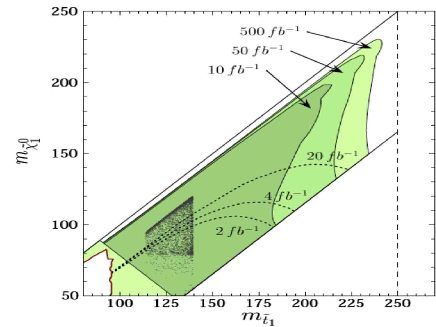
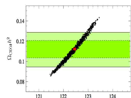
Figure 12: Left: discovery reach of Linear Collider with 500 fb^-1 luminosity at $\sqrt{s}=500$ GeV for production of light stop quarks, $\rm e^{+}e^{-}\to\tilde{t}_{1}\,\bar{\tilde{t}}_{1}\to c\tilde{\chi}^{0}_{1}\,\bar{c}\,\tilde{\chi}^{0}_{1}$. The results are given in the stop vs. neutralino mass plane (in GeV). In the gray shaded region, a 5$\sigma$ discovery is possible. The region where $m_{\tilde{\chi}^{0}_{1}}>m_{\rm\tilde{t}_{1}}$ is inconsistent with a neutralino as Lightest Supersymmetric Particle (LSP), while for $m_{\rm\tilde{t}_{1}}>m_{\rm W}+m_{\rm b}+m_{\tilde{\chi}^{0}_{1}}$ the three-body decay $\rm\tilde{t}_{1}\to W^{+}\bar{b}\tilde{\chi}^{0}_{1}$ becomes accessible and dominant. In the light shaded corner to the lower left, the decay of the top quark into a light stop and neutralino is open. The dark gray dots indicate the region consistent with baryogenesis and dark matter [160]. Also shown are the parameter region excluded by LEP searches [199] (white area in the lower left) and the Tevatron light stop reach [200] (dotted lines) for various integrated luminosities. Also, the discovery reach for different luminosities is shown. Right: computation of dark matter relic abundance $\Omega_{\rm CDM}h^{2}$ taking into account estimated experimental uncertainties for stop, chargino, neutralino sector measurements at future colliders. The black dots corresponds to a scan over the 1$\sigma$ ($\Delta\chi^{2}\leq 1$) region allowed by the expected experimental errors, as a function of the measured stop mass, with the red star indicating the best-fit point. The horizontal shaded bands show the 1$\sigma$ and 2$\sigma$ constraints on the relic density measured by WMAP.

As evident from the figure, the ILC can find light stop quarks for mass differences down to $\Delta m\sim{\cal O}(5\,\,\mathrm{GeV})$, beyond the stop-neutralino coannihilation region. The figure shows also the reach which can be achieved with small total luminosities.

6.4 Stop parameter determination

The discovery of light stops would hint toward the possibility of electroweak baryogenesis and may allow the coannihilation mechanism to be effective. In order to confirm this idea, the relevant supersymmetry parameters need to be measured accurately. In this section, the experimental determination of the stop parameters will be discussed. The mass and its uncertainty has been determined with the polarization method: $m_{\rm\tilde{t}}=122.5\pm 1.0$ GeV.

The mass of the heavier stop $\rm\tilde{t}_{2}$ is too large to be measured directly, but it is assumed that a limit of $m_{\rm\tilde{t}_{2}}>1000$ GeV can be set from collider searches. Combining the stop parameter measurements with corresponding data from the neutralino and chargino sector [157] allows to compute the neutralino dark matter abundance from expected experimental Linear Collider results in the MSSM. All experimental errors are propagated and correlations are taken into account by means of a $\chi^{2}$ analysis. The result of a scan over 100000 random points within the expected experimental uncertainties for this small $\Delta m$ scenario is shown in Fig. 12. The horizontal bands depict the relic density as measured by WMAP [3], which is at 1$\sigma$ level $0.104<\Omega_{\rm CDM}h^{2}<0.121$.

The collider measurements of the stop and chargino/neutralino parameters constrain the relic density to $0.100<\Omega_{\rm CDM}h^{2}<0.124$ at the 1$\sigma$ level, with an overall precision comparable to the direct WMAP determination.

In summary, scalar top quark production and decay at a Linear Collider have been studied with a realistic detector simulation with focus on the c-tagging performance of a CCD vertex detector. The SIMDET simulation includes a CCD vertex detector (LCFI Collaboration). The tagging of c-quarks reduces the background by about a factor 3 in the $\rm c\tilde{\chi}^{0}_{1}\bar{c}\tilde{\chi}^{0}_{1}$ channel. Thus, scalar top processes can serve well as a benchmark reaction for the vertex detector performance.

Dedicated simulations with SPS-5 parameters are performed. The expected background depends significantly on the detector design, mostly on the radius of the inner layer. Similar results have been obtained from simulations of small mass differences between scalar top and neutralino.

For the scalar top mass determination four methods are compared and the polarization method gives the highest precision. The other methods are also important as they contribute to determine the properties of the scalar top quark. For example, the scalar character of the stops can be established from the threshold cross section scan.

A new study for small mass difference, thus small visible energy, shows that a Linear Collider has a large potential to study the scalar top production and decay, in particular in this experimentally very challenging scenario.

From detailed simulations together with estimated errors for measurements in the neutralino and chargino sector [157], the expected cosmological dark matter relic density can be computed. The precision at a Linear Collider will be similar to the current precision of WMAP. The uncertainty in the dark matter prediction from a Linear Collider is dominated by the measurement of scalar top quark mass.

7 CONCLUSIONS

New developments in scalar top studies have been discussed and four sets of Les Houches Scalar top (LHS) benchmarks sets have been defined. The strong cosmological motivation for light scalar top quarks has been review and relevant aspects for the collider searches have been emphasised. The search for scalar top quarks and measuring their properties will be an important task at future colliders. The experimental simulations show that like-sign top signatures could be detected as signals for scalar top production at the LHC. In a second LHC study it has been shown that light scalar tops could be observed already with low luminosity, possibly after a few months of data- taking. For the future Linear Collider aspects of the detector design have been addressed with c-quark tagging as a benchmark for the vertex detector optimization. Different methods of scalar top masses reconstruction have been compared and for cosmological interesting parameter region, the ILC could achieve a similar precision on the relic dark matter density as the current WMAP measurements. Both at the LHC and the ILC, scalar top studies continue to be an active and progressing field of research.

Acknowledgements

Research at the HEP Division of ANL is supported in part by the US DOE, Division of HEP, Contract W-31-109-ENG-38. Fermilab is operated by Universities Research Association Inc. under contract no. DE-AC02-76CH02000 with the DOE.

S.K. is supported by an APART (Austrian Programme of Advanced Research and Technology) grant of the Austrian Academy of Sciences. She also acknowledges the financial support of CERN for the participation at the Les Houches 2005 Workshop. A.R. is supported by the Norwegian Research Council.

T.L and G.P. thank members of the ATLAS Collaboration for helpful discussions. T.L and G.P. have made use of ATLAS physics analysis and simulation tools which are the result of collaboration-wide efforts.

A.S. acknowledges the support from PPARC and Lancaster University grants.

The authors are grateful to the Les Houches workshop organisers for their invitation and support throughout. We also thank S. Heinemeyer and G. Weiglein for useful suggestions.

Part 9 Identifying nonminimal neutralinos in combined LHC and ILC analyses

S. Hesselbach, F. Franke, H. Fraas and G. Moortgat-Pick

1 INTROCUCTION

The Next-to-minimal Supersymmetric Standard Model NMSSM is the simplest extension of the MSSM by an additional Higgs singlet field. It contains five neutralinos $\tilde{\chi}^{0}_{i}$, the mass eigenstates of the photino, zino and neutral higgsinos, and two charginos $\tilde{\chi}^{\pm}_{i}$, being mixtures of wino and charged higgsino. The neutralino/chargino sector depends at tree level on six parameters: the U(1) and SU(2) gaugino masses $M_{1}$ and $M_{2}$, the ratio $\tan\beta$ of the vacuum expectation values of the doublet Higgs fields, the vacuum expectation value $x$ of the singlet field and the trilinear couplings $\lambda$ and $\kappa$ in the superpotential, where the product $\lambda x=\mu_{\rm eff}$ replaces the $\mu$-parameter of the MSSM [201, 202, 203, 204]. The additional fifth neutralino may significantly change the phenomenology of the neutralino sector. In scenarios where the lightest supersymmetric particle is a nearly pure singlino, the existence of displaced vertices may lead to a particularly interesting experimental signature [205, 206, 207, 208] which allows the distinction between the models. If however, only a part of the particle spectrum is kinematically accessible this distinction may become challenging. In this contribution we analyze an NMSSM scenario where the Higgs sector and mass and cross section measurements in the neutralino sector do not allow to distinguish the models, but only a combined analysis of LHC and ILC data.

2 STARTING POINT: NMSSM SCENARIO

We start with an NMSSM scenario with the parameters

$$M_{1}=360\leavevmode\nobreak\ \mbox{\rm GeV},\quad M_{2}=147\leavevmode\nobreak\ \mbox{\rm GeV},\quad\tan\beta=10,\quad\lambda=0.5,\quad x=915\leavevmode\nobreak\ \mbox{\rm GeV},\quad\kappa=0.2.$$ (1)

and the following gaugino/higgsino masses and eigenstates:

$$m_{\tilde{\chi}^{0}_{1}}=138\leavevmode\nobreak\ \mbox{\rm GeV},\quad\quad\tilde{\chi}^{0}_{1}=(-0.02,+0.97,-0.20,+0.09,-0.07),$$ (2)

$$m_{\tilde{\chi}^{0}_{2}}=337\leavevmode\nobreak\ \mbox{\rm GeV},\quad\quad\tilde{\chi}^{0}_{2}=(+0.62,+0.14,+0.25,-0.31,+0.65),$$ (3)

$$m_{\tilde{\chi}^{0}_{3}}=367\leavevmode\nobreak\ \mbox{\rm GeV},\quad\quad\tilde{\chi}^{0}_{3}=(-0.75,+0.04,+0.01,-0.12,+0.65),$$ (4)

$$m_{\tilde{\chi}^{0}_{4}}=468\leavevmode\nobreak\ \mbox{\rm GeV},\quad\quad\tilde{\chi}^{0}_{4}=(-0.03,+0.08,+0.70,+0.70,+0.08),$$ (5)

$$m_{\tilde{\chi}^{0}_{5}}=499\leavevmode\nobreak\ \mbox{\rm GeV},\quad\quad\tilde{\chi}^{0}_{5}=(+0.21,-0.16,-0.64,+0.62,+0.37),$$ (6)

where the neutralino eigenstates are given in the basis $(\tilde{B}^{0},\tilde{W}^{0},\tilde{H}^{0}_{1},\tilde{H}^{0}_{2},\tilde{S})$. As can be seen from Eqs. (3) and (4), the particles $\tilde{\chi}^{0}_{2}$ and $\tilde{\chi}^{0}_{3}$ have a rather strong singlino admixture. This scenario translates at the $e^{+}e^{-}$ International Linear Collider (ILC) with $\sqrt{s}=500$ GeV into the experimental observables of Table 1 for the measurement of the masses and production cross sections for several polarization configurations of the light neutralinos and charginos. We assume mass uncertainties of $\mathcal{O}(1-2\%)$, a polarization uncertainty of $\Delta P_{e^{\pm}}/P_{e^{\pm}}=0.5\%$ and one standard deviation statistical errors. The masses and cross sections in different beam polarization configurations provide the experimental input for deriving the supersymmetric parameters within the MSSM using standard methods [26, 27]. Note that beam polarization may be crucial for distinguishing the two models [209, 210, 211].

Table 1: Masses with 1.5% ($\tilde{\chi}^{0}_{2,3}$, $\tilde{e}_{L,R}$, $\tilde{\nu}_{e}$) and 2% ($\tilde{\chi}^{0}_{1}$, $\tilde{\chi}^{\pm}_{1}$) uncertainty and cross sections with an error composed of the error due to the mass uncertainties, polarization uncertainty of $\Delta P_{e^{\pm}}/P_{e^{\pm}}=0.5\%$ and one standard deviation statistical error based on $\int{\cal L}=100$ fb^-1, for both unpolarized beams and polarized beams with $(P_{e^{-}},P_{e^{+}})=(\mp 90\%,\pm 60\%)$, in analogy to the study in [75].

$\scriptstyle m_{\tilde{\chi}^{0}_{1}}=138\pm 2.8$ GeV		$\sigma(e^{+}e^{-}\to\tilde{\chi}^{\pm}_{1}\tilde{\chi}^{\mp}_{1})$/fb		$\sigma(e^{+}e^{-}\to\tilde{\chi}^{0}_{1}\tilde{\chi}^{0}_{2})$/fb
$\scriptstyle m_{\tilde{\chi}^{0}_{2}}=337\pm 5.1$ GeV	$(P_{e^{-}},P_{e^{+}})$	$\sqrt{s}=400$ GeV	$\sqrt{s}=500$ GeV	$\sqrt{s}=500$ GeV
$\scriptstyle m_{\tilde{\chi}^{\pm}_{1}}=139\pm 2.8$ GeV	Unpolarized	$323.9\pm 33.5$	$287.5\pm 16.5$	$4.0\pm 1.2$
$\scriptstyle m_{\tilde{e}_{L}}=240\pm 3.6$ GeV	$(-90\%,+60\%)$	$984.0\pm 101.6$	$873.9\pm 50.1$	$12.1\pm 3.8$
$\scriptstyle m_{\tilde{e}_{R}}=220\pm 3.3$ GeV	$(+90\%,-60\%)$	$13.6\pm 1.6$	$11.7\pm 1.2$	$0.2\pm 0.1$
$\scriptstyle m_{\tilde{\nu}_{e}}=226\pm 3.4$ GeV

3 SUPERSYMMETRIC PARAMETER DETERMINATION AT THE ILC

For the determination of the supersymmetric parameters in the MSSM straightforward strategies have been worked out even if only the light neutralinos and charginos $\tilde{\chi}^{0}_{1}$, $\tilde{\chi}^{0}_{2}$ and $\tilde{\chi}^{\pm}_{1}$ are kinematically accessible at the first stage of the ILC [26, 27].

Using the methods described in in [212, 213] we derive constraints for the parameters $M_{1}$, $M_{2}$, $\mu$ and $\tan\beta$ in two steps. First, the measured masses and cross sections at two energies in the chargino sector constrain the chargino mixing matrix elements $U_{11}^{2}$ and $V_{11}^{2}$. Adding then mass and cross section measurements in the neutralino sector allows to constrain the parameters

$$M_{1} = 377\pm 42\mbox{ GeV},$$ (7)

$$M_{2} = 150\pm 20\mbox{ GeV},$$ (8)

$$\mu = 450\pm 100\mbox{ GeV},$$ (9)

$$\tan\beta = [1,30].$$ (10)

Since the heavier neutralino and chargino states are not produced, the parameters $\mu$ and $\tan\beta$ can only be determined with a considerable uncertainty.

With help of the determined parameter ranges, Eqs. (7)–(10), the masses of heavier charginos and neutralinos can be calculated:

$$m_{\tilde{\chi}^{0}_{3}}=[352,555]\mbox{ GeV},\quad\quad m_{\tilde{\chi}^{0}_{4}}=[386,573]\mbox{ GeV},\quad\quad m_{\tilde{\chi}^{\pm}_{2}}=[350,600]\mbox{ GeV}.$$ (11)

In Fig. 1 (left panel) the masses of $\tilde{\chi}^{0}_{3}$ and $\tilde{\chi}^{0}_{4}$ are shown as a function of its gaugino admixture for parameter points within the constraints of Eqs. (7)–(10). Obviously, the heavy neutralino $\tilde{\chi}^{0}_{3}$ should be almost a pure higgsino within the MSSM prediction. These predicted properties of the heavier particles can now be compared with mass measurements of SUSY particles at the LHC within cascade decays [75].

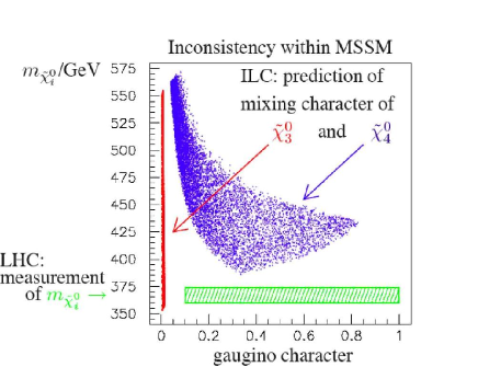
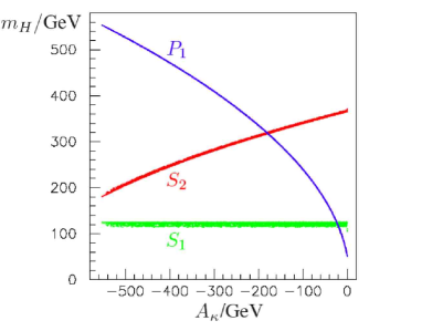
Figure 1: Left: Predicted masses and gaugino admixture for the heavier neutralinos $\tilde{\chi}^{0}_{3}$ and $\tilde{\chi}^{0}_{4}$ within the consistent parameter ranges derived at the ILC₅₀₀ analysis in the MSSM and measured mass $m_{\tilde{\chi}^{0}_{i}}=367\pm 7$ GeV of a neutralino with sufficiently high gaugino admixture in cascade decays at the LHC. We took a lower bound of sufficient gaugino admixture of about 10% for the heavy neutralinos, cf. [214, 215]. Right: The possible masses of the two light scalar Higgs bosons, $m_{S_{1}}$, $m_{S_{2}}$, and of the lightest pseudoscalar Higgs boson $m_{P_{1}}$ as function of the trilinear Higgs parameter $A_{\kappa}$ in the NMSSM. In our chosen scenario, $S_{1}$ is MSSM-like and $S_{2}$ and $P_{1}$ are heavy singlet-dominated Higgs particles.

The Higgs sector of the NMSSM [216, 217] depends on two additional parameters, the trilinear soft scalar mass parameters $A_{\lambda}$ and $A_{\kappa}$. The Higgs bosons with dominant singlet character may escape detection in large regions of these parameters, thus the Higgs sector does not allow the identification of the NMSSM. A scan with NMHDECAY [218] in our scenario, Eq. (1), over $A_{\lambda}$ and $A_{\kappa}$ results in parameter points which survive the theoretical and experimental constraints in the region $2740\leavevmode\nobreak\ \textrm{GeV}<A_{\lambda}<5465$ GeV and $-553\leavevmode\nobreak\ \textrm{GeV}<A_{\kappa}<0$. For $-443\leavevmode\nobreak\ \textrm{GeV}<A_{\kappa}<-91$ GeV the second lightest scalar ($S_{2}$) and the lightest pseudoscalar ($P_{1}$) Higgs particle have very pure singlet character and are heavier than the mass difference $m_{\tilde{\chi}^{0}_{3}}-m_{\tilde{\chi}^{0}_{1}}$, hence the decays of the neutralinos $\tilde{\chi}^{0}_{2}$ and $\tilde{\chi}^{0}_{3}$, which will be discussed in the following, are not affected by $S_{2}$ and $P_{1}$. The dependence of the masses of $S_{1}$, $S_{2}$ and $P_{1}$ on $A_{\kappa}$ is illustrated in Fig. 1 (right panel). The mass of the lightest scalar Higgs $S_{1}$, which has MSSM-like character in this parameter range, depends only weakly on $A_{\kappa}$ and is about 124 GeV. The masses of $S_{3}$, $P_{2}$ and $H^{\pm}$ are of the order of $A_{\lambda}$. For $A_{\kappa}<-443$ GeV the smaller mass of the $S_{2}$ and a stronger mixing between the singlet and MSSM-like states in $S_{1}$ and $S_{2}$ might allow a discrimination in the Higgs sector while for $A_{\kappa}>-91$ GeV the existence of a light pseudoscalar $P_{1}$ may give first hints of the NMSSM [219]. For our specific case study we choose $A_{\lambda}=4000$ GeV and $A_{\kappa}=-200$ GeV, which leads to $m_{S_{2}}=311$ GeV, $m_{P_{1}}=335$ GeV.

We emphasize that although we started with an NMSSM scenario where $\tilde{\chi}^{0}_{2}$ and $\tilde{\chi}^{0}_{3}$ have large singlino admixtures, the MSSM parameter strategy does not fail and the experimental results from the ILC₅₀₀ with $\sqrt{s}=400$ GeV and $500$ GeV lead to a consistent parameter determination in the MSSM. Hence in the considered scenario the analyses at the ILC₅₀₀ or LHC alone do not allow a clear discrimination between MSSM and NMSSM. All predictions for the heavier gaugino/higgsino masses are consistent with both models. However, the ILC₅₀₀ analysis predicts an almost pure higgsino-like state for $\tilde{\chi}^{0}_{3}$ and a mixed gaugino-higgsino-like $\tilde{\chi}^{0}_{4}$, see Fig. 1 (left panel). This allows the identification of the underlying supersymmetric model in combined analyses at the LHC and the ILC${}_{650}^{{\cal L}=1/3}$.

4 COMBINED LHC AND ILC ANALYSIS

In our original NMSSM scenario, Eq. (1), the neutralinos $\tilde{\chi}^{0}_{2}$ and $\tilde{\chi}^{0}_{3}$ have a large bino-admixture and therefore appear in the squark decay cascades. The dominant decay mode of $\tilde{\chi}^{0}_{2}$ has a branching ratio $BR(\tilde{\chi}^{0}_{2}\to\tilde{\chi}^{\pm}_{1}W^{\mp})\sim 50\%$, while for the $\tilde{\chi}^{0}_{3}$ decays $BR(\tilde{\chi}^{0}_{3}\to\tilde{\ell}^{\pm}_{L,R}\ell^{\mp})\sim 45\%$ is largest. Since the heavier neutralinos, $\tilde{\chi}^{0}_{4}$, $\tilde{\chi}^{0}_{5}$, are mainly higgsino-like, no visible edges from these particles occur in the cascades. It is expected to see the edges for $\tilde{\chi}^{0}_{2}\to\tilde{\ell}^{\pm}_{R}\ell^{\mp}$, $\tilde{\chi}^{0}_{2}\to\tilde{\ell}^{\pm}_{L}\ell^{\mp}$, $\tilde{\chi}^{0}_{3}\to\tilde{\ell}^{\pm}_{R}\ell^{\mp}$ and for $\tilde{\chi}^{0}_{3}\to\tilde{\ell}^{\pm}_{L}\ell^{\mp}$. With a precise mass measurement of $\tilde{\chi}^{0}_{1}$,$\tilde{\chi}^{0}_{2}$, $\tilde{\ell}_{L,R}$ and $\tilde{\nu}$ from the ILC₅₀₀ analysis, a clear identification and separation of the edges of the two gauginos at the LHC is possible without imposing specific model assumptions. We therefore assume a precision of about 2% for the measurement of $m_{\tilde{\chi}^{0}_{3}}$, in analogy to [214, 215]:

$$m_{\tilde{\chi}^{0}_{3}}=367\pm 7\mbox{ GeV}.$$ (12)

The precise mass measurement of $\tilde{\chi}^{0}_{3}$ is compatible with the mass predictions of the ILC₅₀₀ for the $\tilde{\chi}^{0}_{3}$ in the MSSM but not with the prediction of the small gaugino admixture, see Fig. 1 (left panel). The $\tilde{\chi}^{0}_{3}$ as predicted in the MSSM would not be visible in the decay cascades at the LHC. The other possible interpretation of the measured neutralino as the $\tilde{\chi}^{0}_{4}$ in the MSSM is incompatible with the cross section measurements at the ILC. We point out that a measurement of the neutralino masses $m_{\tilde{\chi}^{0}_{1}}$, $m_{\tilde{\chi}^{0}_{2}}$, $m_{\tilde{\chi}^{0}_{3}}$ which could take place at the LHC alone is not sufficient to distinguish the SUSY models since rather similar mass spectra could exist [212, 213]. Therefore the cross sections in different beam polarization configurations at the ILC have to be included in the analysis.

The obvious inconsistency of the combined results from the LHC and the ILC₅₀₀ analyses and the predictions for the missing chargino/neutralino masses could motivate the immediate use of the low-luminosity but higher-energy option ILC${}_{650}^{{\cal L}=1/3}$ in order to resolve model ambiguities even at an early stage of the experiment and outline future search strategies at the upgraded ILC at 1 TeV. This would finally lead to the correct identification of the underlying model. The expected polarized and unpolarized cross sections, including the statistical error on the basis of one third of the luminosity of the ILC₅₀₀, are given in Table 2. The neutralino $\tilde{\chi}^{0}_{3}$ as well as the higgsino-like heavy neutralino $\tilde{\chi}^{0}_{4}$ and the chargino $\tilde{\chi}^{\pm}_{2}$ are now accessible at the ILC${}^{{\cal L}=1/3}_{650}$. The cross sections together with the precisely measured masses $m_{\tilde{\chi}^{0}_{4}}$ and $m_{\tilde{\chi}^{\pm}_{2}}$ would constitute the observables necessary for a fit of the NMSSM parameters. In order to archive this the fit program Fittino [220] will be extended to include also the NMSSM [221].

Table 2: Expected cross sections for the associated production of the heavier neutralinos and charginos in the NMSSM scenario for the ILC${}^{{\cal L}=1/3}_{650}$ option with one sigma statistical error based on $\int{\cal L}=33$ fb^-1 for both unpolarized and polarized beams.

	$\scriptstyle\sigma(e^{+}e^{-}\to\tilde{\chi}^{0}_{1}\tilde{\chi}^{0}_{j})/$fb at $\scriptstyle\sqrt{s}=650$ GeV			$\scriptstyle\sigma(e^{+}e^{-}\to\tilde{\chi}^{\pm}_{1}\tilde{\chi}^{\mp}_{2})/$fb
	$\scriptstyle j=3$	$\scriptstyle j=4$	$\scriptstyle j=5$	at $\scriptstyle\sqrt{s}=650$ GeV
Unpolarized beams	$\scriptstyle 12.2\pm 0.6$	$\scriptstyle 5.5\pm 0.4$	$\scriptstyle\leq 0.02$	$\scriptstyle 2.4\pm 0.3$
$\scriptstyle(P_{e^{-}},P_{e^{+}})=(-90\%,+60\%)$	$\scriptstyle 36.9\pm 1.1$	$\scriptstyle 14.8\pm 0.7$	$\scriptstyle\leq 0.07$	$\scriptstyle 5.8\pm 0.4$
$\scriptstyle(P_{e^{-}},P_{e^{+}})=(+90\%,-60\%)$	$\scriptstyle 0.6\pm 0.1$	$\scriptstyle 2.2\pm 0.3$	$\scriptstyle\leq 0.01$	$\scriptstyle 1.6\pm 0.2$

5 CONCLUSIONS

We have presented an NMSSM scenario where the measurement of masses and cross sections in the neutralino and chargino sector as well as measurements in the Higgs sector do not allow a distinction from the MSSM at the LHC or at the ILC₅₀₀ with $\sqrt{s}=500$ GeV alone. Precision measurements of the neutralino branching ratio into the lightest Higgs particle and of the mass difference between the lightest and next-to-lightest SUSY particle may give first evidence for the SUSY model but are difficult to realize in our case. Therefore the identification of the underlying model requires precision measurements of the heavier neutralinos by combined analyses of LHC and ILC and the higher energy but lower luminosity option of the ILC at $\sqrt{s}=650$ GeV. This gives access to the necessary observables for a fit of the underlying NMSSM parameters.

Acknowledgements

S.H. and G.M.-P. thank the organizers of Les Houches 2005 for the kind invitation and the pleasant atmosphere at the workshop. We are very grateful to G. Polesello and P. Richardson for constructive discussions. S.H. is supported by the Göran Gustafsson Foundation. This work is supported by the European Community’s Human Potential Programme under contract HPRN-CT-2000-00149 and by the Deutsche Forschungsgemeinschaft (DFG) under contract No. FR 1064/5-2.

Part 10 Electroweak observables and split SUSY at future colliders

J. Guasch and S. Peñaranda

1 INTRODUCTION

Recently, the scenario of Split SUSY has been proposed [222, 223, 224]. In this scenario, the SUSY-breaking scale is much heavier than the electroweak scale, and there is a hierarchy between the scalar superpartners and the fermionic partners of the Standard Model (SM) particles. Except for one Higgs-boson, all scalar particles (squarks, sleptons and extra Higgs particles) are heavy, ${\cal O}(10^{9}\,\,\mathrm{GeV})$, while the fermions (gauginos and higgsinos) are kept at the electroweak scale. Only the SM spectrum, including one Higgs scalar, and gauginos and higgsinos remain. The rest of the Minimal Supersymmetric Standard Model (MSSM) spectrum decouples [225, 226]. This scenario implies the existence of an “unnatural” fine-tuning, such that the Higgs-boson vacuum expectation value can be kept at the observed electroweak scale. Assuming this fine-tuning effect, some of the remaining problems in SUSY models are solved: there is no flavour-changing neutral current problem, and the mediating proton decay problem has been eliminated. On the other hand, keeping gauginos and higgsinos at the electroweak scale, gauge unification is preserved and the neutralino is a good candidate for dark matter. Phenomenological implications of Split SUSY have been extensively discussed during the last year (see e.g. [227]).

In this work we focus on the precision electroweak (EW) observables, specifically on $M_{W}$, $\sin^{2}\theta_{\mathrm{eff}}$, and their correlations. We compare the predictions in Split SUSY with the SM and the MSSM, and study the feasibility of measuring the contributions of Split SUSY at future colliders: the Large Hadron Collider (LHC) and the International $e^{+}e^{-}$ Linear Collider (ILC) – for further details see Ref. [228].

Previous works on precision EW observables in Split SUSY exist. Reference [229] analyzes the $S$, $T$, $U$ parameter expansions, as well as corrections from non-zero momentum summarized in $Y$, $V$, $W$ parameters [230, 231, 232]. They found that the precision electroweak data are compatible with the Split SUSY spectrum for the values of gaugino and higgsino masses above the direct collider limits. Reference [233] studies Split SUSY corrections to precision observables including LEP2 data. The authors of Refs.[229, 233] focus on the analysis of current experimental data, performing a $\chi^{2}$ fit, and finding whether Split SUSY fits better current experimental data than the SM. Our work focusses on the possibility of detecting the deviations induced by Split SUSY in the future measurements of $M_{W}$ and $\sin^{2}\theta_{\mathrm{eff}}$.

2 $M_{W}$ AND $\sin^{2}\theta_{\mathrm{eff}}$ ELECTROWEAK PRECISION OBSERVABLES

The analysis of virtual effects of the non-standard particles on new physics models to precision observables requires a high precision of the experimental results as well as of the theoretical predictions. The leading order radiative corrections to the observables under study can be written as

$$\delta M_{W}\approx\frac{M_{W}}{2}\frac{\cos^{2}\theta_{W}}{\cos^{2}\theta_{W}-\sin^{2}\theta_{W}}\Delta\rho,\quad\delta\sin^{2}\theta_{\mathrm{eff}}\approx-\frac{\cos^{2}\theta_{W}\sin^{2}\theta_{W}}{\cos^{2}\theta_{W}-\sin^{2}\theta_{W}}\Delta\rho\,,$$ (1)

$\theta_{W}$ being the weak mixing angle, and $\Delta\rho={\Sigma_{Z}(0)}/{M_{Z}^{2}}-{\Sigma_{W}(0)}/{M_{W}^{2}}$, with $\Sigma_{Z,W}(0)$ the unrenormalized $Z$ and $W$ boson self-energies at zero momentum. Beyond the $\Delta\rho$ approximation, the shifts in these two observables are given in terms of the $\delta(\Delta r)$ quantity. The computation of $\Delta r$ in Split SUSY reduces to the computation of gauge bosons self-energies.

For our computation, we have used ZFITTER [234, 235] for the SM prediction. The MSSM contributions to $\Delta r$ have been taken from Ref. [236, 237, 238, 239], and we have used FeynArts/FormCalc/LoopTools [240, 241, 242, 243, 244, 245] for the vertex contributions to $\sin^{2}\theta_{\mathrm{eff}}$. The Higgs-boson mass is computed according to Ref. [223] for Split SUSY, and using the leading $m_{t}$, $m_{b}\tan\beta$ approximation for the MSSM [246, 247, 248, 249]. The Split SUSY/MSSM contributions to $\Delta r$ are added to the ZFITTER computation, and we proceed in an iterative way to compute $M_{W},\sin^{2}\theta_{W}$. As for the input parameters, we have used $M_{Z}=91.1876\,\,\mathrm{GeV}$, $\alpha^{-1}(0)=137.0359895$ [48], $\Delta\alpha^{5}_{\rm had}(M_{Z})=0.02761\pm 0.00036$ [250] (corresponding to $\alpha^{-1}(M_{Z})=128.936$), $\alpha_{s}(M_{Z})=0.119\pm 0.003$ [250]. For the top-quark mass, we use the latest combination of RunI/II Tevatron data: $m_{t}=172.7\pm 2.9\,\,\mathrm{GeV}$ [251].

The parameter space of Split SUSY is formed by the higgsino mass parameter $\mu$, the electroweak gaugino soft-SUSY-breaking mass parameters $M_{1}$ and $M_{2}$ (we use the GUT mass relation $M_{1}=M_{2}\,5/3\,\tan^{2}\theta_{W}$), the gluino soft-SUSY-breaking mass $M_{g}$, the ratio between the vacuum expectation values of the two Higgs doublets $\tan\beta=v_{2}/v_{1}$, and the scale of the scalar particles masses $\tilde{m}$. The scalar mass scale ($\tilde{m}$) lays between the EW scale ($\sim 1\,\,\mathrm{TeV}$) and the unification scale ($\sim 10^{16}\,\,\mathrm{GeV}$), current limits from gluino cosmology set an upper bound $\tilde{m}\lesssim 10^{9}\,\,\mathrm{GeV}$ [252]. In our computation the gluino mass ($M_{g}$) and the scalar scale ($\tilde{m}$) enter the Higgs-boson mass computation, the latter defining the matching scale with the SUSY theory, and the former through the running of the top quark Yukawa coupling. For definiteness, we will use $\tilde{m}=10^{9}\,\,\mathrm{GeV}$, while $M_{g}$ is let free.

3 RESULTS

Now we focus on the comparison for $M_{W}$ and $\sin^{2}\theta_{\mathrm{eff}}$ predictions from different models with the present data and the prospective experimental precision. The results for the SM, the MSSM and Split SUSY predictions are given in Fig. 1, in the $M_{W}$–$\sin^{2}\theta_{\mathrm{eff}}$ plane. The top-quark mass is varied in the $3\sigma$ range of the experimental determination. Predictions are shown together with the experimental results for $M_{W}$ and $\sin^{2}\theta_{\mathrm{eff}}$ ($M_{W}=80.410\pm 0.032\,\,\mathrm{GeV}\,,\,\sin^{2}\theta_{\mathrm{eff}}=0.231525\pm 0.00016$) and the prospective accuracies at present (LEP2, SLD, Tevatron) and at the next generations of colliders (LHC, ILC, GigaZ) [253, 254]. Our results agree with previous ones for the SM and the MSSM predictions given in [255, 256, 257].

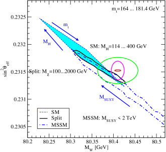
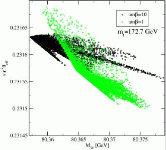
(a)	(b)

Figure 1: a) SM, MSSM and Split SUSY predictions for $M_{W}$ and $\sin^{2}\theta_{\mathrm{eff}}$. The ellipses are the experimental results for $M_{W}$ and $\sin^{2}\theta_{\mathrm{eff}}$ and the prospective accuracies at LEP2/SLD/Tevatron (large ellipse), LHC/ILC (medium ellipse) and GigaZ (small ellipse). b) Prediction of $M_{W}$ and $\sin^{2}\theta_{\mathrm{eff}}$ from a parameter scan in the Split SUSY parameter space with $m_{t}=172.7\,\,\mathrm{GeV}$ and $\tan\beta=1$ (green/light-grey area) and $\tan\beta=10$ (black area).

We have performed a Monte Carlo scan of the parameter space of the different models, taking into account experimental limits on new particles, to find the allowed region in the $M_{W}$–$\sin^{2}\theta_{\mathrm{eff}}$ plane for each model. The results are shown in Fig. 1a. The allowed regions are those enclosed by the different curves. The arrows show the direction of change in these regions as the given parameters grow. The shaded region corresponds to the SM prediction, and it arises from varying the mass of the SM Higgs-boson, from $114\,\,\mathrm{GeV}$ [133] to $400\,\,\mathrm{GeV}$. The region enclosed by the dash-dotted curve corresponds to the MSSM. The SUSY masses are varied between $2\,\,\mathrm{TeV}$ (upper edge of the area) and close to their experimental lower limit $m_{\chi}\gtrsim 100\,\,\mathrm{GeV}$, $m_{\tilde{f}}\gtrsim 150\,\,\mathrm{GeV}$ (lower edge of the band). The overlap region between SM and MSSM corresponds to the region where the Higgs-boson is light, i.e. in the MSSM allowed region $m_{h^{0}}<140\,\,\mathrm{GeV}$ [257], all superpartners being heavy [255, 256]. The Split SUSY region is enclosed by the black line in this figure. The computed Higgs-boson mass varies in the range $m_{H}^{\rm split}\sim 110$–$153\,\,\mathrm{GeV}$. As expected, we found overlap regions between Split SUSY and both the SM and the MSSM. Moreover, we see that most of the region predicted by Split SUSY for $M_{W}$ and $\sin^{2}\theta_{\mathrm{eff}}$ overlaps with predictions already given by the SM and the MSSM.

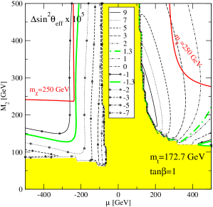
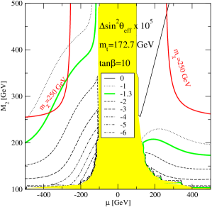
(a)	(b)
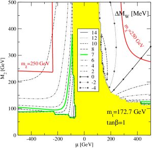
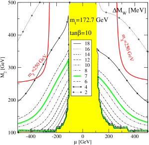
(c)	(d)

Figure 2: The shifts $\Delta\sin^{2}\theta_{\mathrm{eff}}$ and $\Delta M_{W}$ in the $[M_{2}$–$\mu]$ plane for $m_{t}=172.7\,\,\mathrm{GeV}$ and for $\tan\beta=1$ (a, c) and $\tan\beta=10$ (b, d). The shaded region corresponds to $m_{\chi}<100\,\,\mathrm{GeV}$. Also shown is the line corresponding to a lightest chargino mass $m_{\chi}=250\,\,\mathrm{GeV}$. The gluino mass is taken to be $M_{g}=500\,\,\mathrm{GeV}$.

From now on, we focus on the differences between SM and Split SUSY predictions. To assess the importance of the Split SUSY contributions, we must compare these with the present and future experimental uncertainties and SM theoretical errors. The current experimental uncertainties are [258, 259]

$$\Delta M_{W}^{\rm exp,today}\approx 34\,\,\mathrm{MeV},\qquad\Delta\sin^{2}\theta_{\mathrm{eff}}^{\rm exp,today}\approx 17\times 10^{-5}\,;$$ (2)

the expected experimental precision for the LHC is [260]

$$\Delta M_{W}^{\rm LHC}\approx 15\mbox{--}20\,\,\mathrm{MeV}\,\,;$$ (3)

and at GigaZ one expects [261, 262, 263, 264, 253]

$$\Delta M_{W}^{\rm exp,future}\approx 7\,\,\mathrm{MeV},\qquad\Delta\sin^{2}\theta_{\mathrm{eff}}^{\rm exp,future}\approx 1.3\times 10^{-5}\leavevmode\nobreak\ .$$ (4)

On the other hand, the theoretical intrinsic uncertainties in the SM computation are [257]:

$$\Delta M_{W}^{\rm th,today,SM}\approx 4\,\,\mathrm{MeV}, \Delta\sin^{2}\theta_{\mathrm{eff}}^{\rm th,today,SM}\approx 5\times 10^{-5}\leavevmode\nobreak\ ,$$

$$\Delta M_{W}^{\rm th,future,SM}\approx 2\,\,\mathrm{MeV}, \Delta\sin^{2}\theta_{\mathrm{eff}}^{\rm th,future,SM}\approx 2\times 10^{-5}\leavevmode\nobreak\ .$$ (5)

Figure 1b shows the result of the parameter scan in Split SUSY for two values of $\tan\beta$. The effective leptonic weak mixing angle, $\sin^{2}\theta_{\mathrm{eff}}$, always decreases when $\tan\beta=10$ but, on the contrary, its value increases when $\tan\beta=1$ for some specific set of values of the other parameters, in particular when $\mu>0$ (see below). The correction to $\sin^{2}\theta_{\mathrm{eff}}$ is positive for small values of $\tan\beta$ and $\mu>0$. The corrections to $M_{W}$ are positive over a large range of the parameter space. When $\tan\beta=1$ and $\mu>0$ we can also get negative corrections. For values of $\tan\beta>10$ the above conclusions remain unchanged.

In Fig. 2 we show the shifts $\Delta\sin^{2}\theta_{\mathrm{eff}}$ and $\Delta M_{W}$ in the $[M_{2}$–$\mu]$ plane. The shifts in the variables are defined as: $\Delta X\equiv X^{\rm Split\ SUSY}-X^{\rm SM}$, where the SM computation is performed using the Higgs-boson mass predicted by Split SUSY. The Split-SUSY-induced shifts are $|\Delta\sin^{2}\theta_{\mathrm{eff}}|<10\times 10^{-5}$ and $|\Delta M_{W}|<20\,\,\mathrm{MeV}$; as for today’s data (2) they are smaller than the experimental error, and the data cannot discriminate between the SM and Split SUSY. The same conclusion applies to the accuracy reached at the LHC (3). However, the shifts are larger than the experimental accuracy of GigaZ (4) in certain regions of the parameter space. For $\tan\beta=1$, the shift in $|\Delta\sin^{2}\theta_{\mathrm{eff}}|$ is larger than $1.3\times 10^{-5}$ for most of the explored region for $\mu>0$ and for the region with $\mu<0$: $\mu\gtrsim-250\,\,\mathrm{GeV}$ or $M_{2}\lesssim 150\,\,\mathrm{GeV}$ (Fig. 2a). At $\tan\beta=10$ (Fig. 2b), $|\Delta\sin^{2}\theta_{\mathrm{eff}}|$ is larger than the future experimental accuracy (4) in a small region $M_{2}\lesssim 175$–$200\,\,\mathrm{GeV}$ for $\mu>0$, and a large region $M_{2}\lesssim 200$–$500\,\,\mathrm{GeV}$ for $\mu<0$. As far as $M_{W}$ is concerned, the LHC measurement (3) could only be useful in a small corner of the parameter space for $\mu<0$, $\tan\beta\;\raisebox{-3.00003pt}{$\stackrel{{\scriptstyle\displaystyle>}}{{\sim}}$}\;10$. The GigaZ measurement (4) does not help for $\tan\beta=1$, $\mu>0$. For $\tan\beta=1$, $\mu<0$ there exists a small region for $M_{2}\lesssim 110\,\,\mathrm{GeV}$ or $\mu>-110\,\,\mathrm{GeV}$. For larger $\tan\beta$, the region of sensitivity is much larger. Summarizing the results of Fig. 2:

• Positive shifts of $\sin^{2}\theta_{\mathrm{eff}}$ are only possible at small $\tan\beta\simeq 1$ and $\mu>0$. They are large, and correlated with small and negative shifts of $M_{W}$. These large shifts are possible even for large values of the chargino masses ($m_{\chi}>250\,\,\mathrm{GeV}$).

• For $\tan\beta\simeq 1$, $\mu<0$ large negative shifts in $\sin^{2}\theta_{\mathrm{eff}}$ are possible, correlated with positive shifts in $M_{W}$, but $\sin^{2}\theta_{\mathrm{eff}}$ is the most sensitive of those observables.

• For large $\tan\beta\gtrsim 10$ and $\mu>0$, the sensitivity region is confined to small $M_{2}\lesssim 275$–$375\,\,\mathrm{GeV}$, with the largest shift provided by $\sin^{2}\theta_{\mathrm{eff}}$ for $\mu\gtrsim 300\,\,\mathrm{GeV}$, and by $M_{W}$ otherwise.

• Finally, for large $\tan\beta\gtrsim 10$ and $\mu<0$, the largest sensitivity is provided by $\sin^{2}\theta_{\mathrm{eff}}$; it can reach GigaZ sensitivities even for moderate chargino masses ($m_{\chi}\approx 250\,\,\mathrm{GeV}$).

We would like to stress that the results for negative $\mu$ are quite different from those of positive $\mu$. As Fig. 2 shows, changing the sign of $\mu$ can change the sign and the absolute value of the shifts significantly.

The results of the difference between Split SUSY and SM predictions in the $M_{W}$–$\sin^{2}\theta_{\mathrm{eff}}$ plane are displayed in Fig. 3, together with the expected error ellipses of the future colliders (3) and (4) centered at the SM value. We can see that the shift $\Delta M_{W}$ can be up to $23\,\,\mathrm{MeV}$ at its maximum and it is impossible to discriminate between models at present. However, future experiments could be probed with the future precision on $M_{W}$. On the other hand, the shifts $\Delta\sin^{2}\theta_{\mathrm{eff}}$ can easily reach values $\pm 2\times 10^{-5}$, which is larger than both the expected experimental errors and the anticipated theoretical accuracies (5).

We observe from Fig. 1a that the current SM prediction of $M_{W}$–$\sin^{2}\theta_{\mathrm{eff}}$ would need a positive shift on both observables (together with a large value of $m_{t}$) to be closer to the central experimental value. Figs. 2, 3 show that the general trend of the Split SUSY contributions is a negative correlation of the shifts on both observables. The region providing ($\Delta M_{W}>0$, $\Delta\sin^{2}\theta_{\mathrm{eff}}>0$) is actually small and the largest region corresponds to ($\Delta M_{W}>0$, $\Delta\sin^{2}\theta_{\mathrm{eff}}<0$) –c.f. Fig. 3. Of course, small deviations from the general trend are important, and Refs. [229, 233] show that there are points of the parameter Split SUSY space that fit better than the SM the experimental value of the electroweak precision observables.

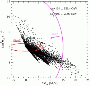
Figure 3: Shifts of the differences between Split SUSY and SM predictions for $M_{W}$ and $\sin^{2}\theta_{\mathrm{eff}}$, scanning over the parameter space. Also shown are the ellipses for the prospective accuracies at LHC/ILC (large ellipse) and GigaZ (small ellipse).

4 CONCLUSIONS

We find that the shifts induced in Split SUSY models are smaller than present experimental accuracies (2), and no conclusion can be drawn with respect to the validity of this model. With the anticipated LHC accuracy on $M_{W}$, a small corner of the parameter space can be explored. However, only with the GigaZ option of the ILC would the experiment be sensitive to the Split SUSY corrections to these observables. In this option, the effective leptonic mixing angle ($\sin^{2}\theta_{\mathrm{eff}}$) is the most sensitive of the two observables. For moderate and large $\tan\beta$, the lightest chargino must be relatively light, $m_{\chi}\lesssim 250\,\,\mathrm{GeV}$, and will already have been detected either at the LHC or the ILC before the GigaZ era. The observables provide, however, a high-precision test of the model. An interesting case is a scenario with low $\tan\beta\simeq 1$ and positive $\mu$, where large shifts in $\sin^{2}\theta_{\mathrm{eff}}$ are expected, even for large values of the chargino masses.

Acknowledgements

The work of S.P. has been supported by the European Union under contract No. MEIF-CT-2003-500030, and that of J.G. by a Ramon y Cajal contract from MEC (Spain) and in part by MEC and FEDER under project 2004-04582-C02-01 and Generalitat de Catalunya project 2005SGR00564. S.P. is thankful for the warm hospitality at Les Houches 2005.

Part 11 Split supersymmetry with Dirac gaugino masses

K. Benakli

1 INTRODUCTION

Our knowledge of physics at energies above the electroweak scale leaves the door open to different ideas (extra-dimensions, compositeness…). The only constraints come on the LEP precision measurements and mathematicla consistency. Fortunately, there are a few observations which can serve as guidelines for building extensions to the Standard Model (SM), as the necessity of a Dark Matter (DM) candidate and the fact that LEP data favor the unification of the three gauge couplings. Both find natural realization in specific supersymmetric models as the Minimal Supersymetric Standard Model (MSSM). Supersymmetry is also welcome as it naturally arises in string theory, which provides a framework for incorporating the gravitational interaction in our quantum picture of the universe.

The failure to find a dynamical explanation of the very tiny dark energy in the universe, as indicated by recent observations, raises questions on our understanding of the notion of “naturalness”. It raises the possibility that even the gauge hierarchy problem is not solved by a symmetry. Supersymmetry could be present at very high energies and its breaking could lead to a hierarchy between the masses of the different superpartners such as in the so-called split supersymmetry scenario [222, 223]. One of its imprtant features is that even making squarks and sleptons heavy, it is possible to keep successful unification and the existence of a DM candidate. Moreover, constraints related to its complicated scalar sector disappear.

Implementing this idea in string theory has been discussed in [265]. In this work we show that there is an economical string-inspired brane models that allows for unification of gauge couplings at scales safe from proton decay problems and provides us with a natural dark matter candidate.

This work is based on [266].

2 MAIN FEATURES OF THE MODEL

The starting point of the construction is a supersymmetric extension of the standard model. This differs from the minimal extension (MSSM) and is as follows:

• Gauge bosons arise in $N=2$ or $N=4$ supermultiplets which are decomposed, for each gauge group factor $G_{a}$, into one $N=1$ vector superfield $W_{a}$ and one or three chiral adjoint superfields $A_{a}$, respectively.

• Quarks and leptons belong to $N=1$ chiral multiplets.

• Pairs of Higgs doublets originate as $N=1$ chiral multiplets for light Binos Dirac masses and in $N=2$ supersymmetry hypermultiplets otherwise, as we will explain below.

These features have a natural realization in brane constructions: Gauge bosons emerge as massless modes living on the bulk of a stack of coincident branes. Quarks and leptons are identified with massless modes localized at point-like brane intersections. The Higgs doublets are localized in two tori where branes intersect, while they propagate freely in the third torus where the two brane stacks are parallel.

We will asume that supersymmetry is broken by a $D$-term. This is achieved in the brane construction through deforming brane intersections with a small angle $\Theta$ leading to the $D$-term $\langle D\rangle=\Theta M_{S}^{2}$ associated to a corresponding magnetized $U(1)$ factor with superfield strength ${\mathcal{W}}$(see for example [267]). Here, $M_{S}$ is the string scale. This results in soft masses:

• A tree-level mass $m_{0}\propto\sqrt{\Theta}M_{S}$ for squarks and sleptons localized at the deformed intersections. All other scalars acquire in general high masses of order $m_{0}$ by one loop radiative corrections. However an appropriate fine-tuning is needed in the Higgs sector to keep $n_{H}$ doublets light.

• A Dirac mass [268] is induced through the dimension-five operator,

  $$\frac{a}{M_{S}}\int d^{2}\theta{\mathcal{W}}\,W^{a}A_{a}\ \Rightarrow m^{D}_{1/2}\sim a\frac{m_{0}^{2}}{M_{S}}\,,$$ (1)

where $a$ accounts for a possible loop factor.

Actually, this operator (1) might not be present at tree-level and needs to be generated through a loop diagram. In this case, we assume the existence of a “messenger “ sector with the following properties:

• The messenger states form $N=2$ hypermultiplets with a supersymmetric mass $M_{X}$.

• the scalars have masses $M^{2}_{X}\pm m_{0}^{2}$ where the splitting is induced by the supersymmetry breaking.

At one-loop a Dirac gaugino mass is induced:

$$m^{D}_{1/2}\sim\alpha\frac{M_{X}}{M_{s}}\times\frac{m_{0}^{2}}{M_{s}}$$ (2)

where $\alpha$ is the corresponding gauge coupling. An explicit computation in string models gives at first order in $\frac{m_{0}^{2}}{M_{s}^{2}}$ [269]:

$$m_{1/2}^{D}\sim\alpha\frac{m_{0}^{2}}{M_{s}}\int_{0}^{\infty}\frac{dt}{t}\sum_{n}\left({nR_{5}M_{s}}+\frac{M_{X}}{M_{s}}\right)e^{-2\pi t({nR_{5}M_{s}}+\frac{M_{X}}{M_{s}})^{2}}$$ (3)

where the $n=0$ sector reproduces the field theory results.

An important feature is that this mass does not break $R$-symmetry and provides a way out to difficulties with generating gaugino masses for split supersymmetry models.

3 CONSTRAINTS FROM UNIFICATION

For the purpose of studying the unification of gauge couplings some simplifications are in order. First we assume equality of gluinos with winos masses $m^{D}_{1/2}$ and we assume universality of all scalar mass $m_{0}$, except for $n_{H}$ Higgs doublets that remain light at the electroweak scale. Moreover, we use $M_{S}\sim M_{GUT}$ and take $a$ between $1/100\leq a\leq 1$. Our results are given in Table 1.

	$n_{H}$	$a$	$M_{GUT}$	$m_{0}$	$m_{1/2}^{D}$
$N=2$	$1$	$1$	$2.8\times 10^{18}$	$4.5\times 10^{12}$	$7.2\times 10^{6}$
	$1$	$1/100$	$3.8\times 10^{18}$	$3.2\times 10^{13}$	$2.7\times 10^{6}$
	$2$	$1$	$4.5\times 10^{16}$	$1.1\times 10^{13}$	$2.7\times 10^{9}$
	$2$	$1/100$	$4.5\times 10^{16}$	$8.6\times 10^{13}$	$1.6\times 10^{9}$
$N=4$	$1$	$1$	$9.7\times 10^{18}$	$8.5\times 10^{15}$	$7.4\times 10^{12}$
	$1$	$1/100$	$10^{19}$	$6.8\times 10^{16}$	$3.4\times 10^{12}$
	$2$		—	—	—

Table 1: Values for the unification scale $M_{GUT}$, scalar masses $m_{0}$ and Dirac gaugino masses $m_{1/2}^{D}$ in GeV for $N=2,4$ supersymmetric gauge sector, $n_{H}=1,2$ light Higgses, and varying the loop factor $a$.

The results are always stable under the variation of the loop factor $a$. While the number of parameters seems enough to always insure unification, the required values are not always realistic and (perfect) one-loop unification is for instance not possible for $N=4$ and $n_{h}=2$. This might be achieved in refined analysis which would take into account different threshold corrections, as well as the contribution from the messenger sector described above, when present. In fact, these effects can be important for models with low $M_{X}$ or with large compactification volume.

Nice features of the results are: (i) the unification scale lies at values which make the model safe of problems with proton decay, (ii) for $n_{H}=1$ it is compatible with simultaneous unification with gravitationnal interactions without resorting to unknown large threshold corrections.

4 CONSTRAINTS ON BINO MASSES FROM DARK MATTER

The masses of Binos are not constrained by unification requirements, but by the assumption that the neutralino provides an important fraction of the observed dark matter in the universe. Quasi-Dirac Higgsinos interact inelastically with matter via vector-like couplings and direct detection experiments put a lower bound on their mass of order 50 TeV. Pure higgsinos can not make a good dark matter.

A sizeable mixing with Binos must be introduced through the EW symmetry breaking. This is of order $m_{W}^{2}/m_{1/2}^{D}$ and implies an upper bound on the Dirac Bino mass of about $10^{5}$ GeV. Only the case with $N=2$, $n_{H}=1$ case is close to this value. For the other cases one needs a big supression factor is needed. One can play with the factor $M_{X}/M_{s}$ in (3), however in that case it is necessary to ensure that the messenger sector does not modify the unification results. This can be achieved for instance if these states form complete representations of $SU(5)$. Moreover, the Higgs should be in $N=1$ multiplets only in order to destroy the Dirac nature of the Higgsino mass.

We can instead ask that no $m_{1/2}^{D}$ is generated for Binos, but only for the other gauginos. For instance, this is obtained when the messenger sector carry no hypercharge. In this case we use instead Majorana masses generated at two-loop and corresponding to the dimension-seven effective operator [270]:

$$\frac{b^{2}}{M_{S}^{3}}\int d^{2}\theta{\mathcal{W}}^{2}{\rm Tr}W^{2}\Rightarrow m_{1/2}^{M}\sim b^{2}\frac{m_{0}^{4}}{M_{S}^{3}}\,,$$ (4)

where $b$ is a loop factor. This gives $m^{M}_{1/2}\sim 5\times 10^{6}$ GeV for the $N=4$ $n_{H}=1$ model and $m^{M}_{1/2}\sim 100$ GeV for the $N=2$ $n_{H}=2$ model. For the $N=2$ $n_{H}=1$ case, $m^{M}_{1/2}\sim 10$ keV is too small and a Bino Dirac mass is necessary.

5 HIGGSINOS AND NEUTRALINOS MASSES

In the cases with $n_{H}=1$ and $N=4$ or $N=2$, $\mu$ is an independent parameter. It can be associated with the separation of the branes in the torus where they are parallel. The dark matter candidate is mainly a Higgsino mixing with a much heavier Bino . The relic density reproduces the actual WMAP results for $\mu\sim 1.1$ TeV.

Instead, for the $N=2$ $n_{H}=2$ the Higgsinos are in $N=2$ multiplets and the dimension-seven operator,

$$\frac{c}{M_{S}^{3}}\int d^{2}\theta\mathcal{W}^{2}\overline{D}^{2}{\bar{H}}_{1}{\bar{H}}_{2}\Rightarrow\mu\sim c\frac{m_{0}^{4}}{M_{S}^{3}}\,,$$ (5)

where $c$ is again a loop factor, induces the desired mass (of the same order as $m_{1/2}^{M}$ of Eq. (4)). In fact, masses of this order can be shown to be induced at one-loop by the messenger sector through explicit string computation in D-brane constructions  [269]. Electroweak symmetry breaking leads then to the neutralino mass matrix:

$$\left(\begin{array}[]{cccc}M&0&m_{z}s_{w}c_{\beta}&m_{z}s_{w}s_{\beta}\\ 0&M&-m_{z}s_{w}s_{\beta}&m_{z}s_{w}c_{\beta}\\ m_{z}s_{w}c_{\beta}&-m_{z}s_{w}s_{\beta}&0&-\mu\\ m_{z}s_{w}s_{\beta}&m_{z}s_{w}c_{\beta}&-\mu&0\\ \end{array}\right)$$

in the basis $({\tilde{B}}_{1},{\tilde{B}}_{2},{\tilde{H}}_{1},{\tilde{H}}_{2})$ and where $M=m_{1/2}^{M}$ stands for the Bino Majorana masses. The mass matrix can be diagonalized to obtain:

$$m_{\chi}=1/2\left[(M+\epsilon_{1}\mu)-\epsilon_{2}\sqrt{(M-\epsilon_{1}\mu)^{2}+4m_{z}^{2}s_{w}^{2}}\right]$$ (6)

where the four neutralinos with different mass eigenvalues are labeled by $\epsilon_{1,2}=\pm 1$.

As for  [223], we distinguishe three cases:

• $M\ll\mu$: is exculded as the Bino does not interact strongly enough to annihilate and would overclose the universe.

• $M\gg\mu$: WMAP data require $\mu\sim 1.1$ TeV.

• $M\sim\mu$: the lightest neutralino ($\chi$), a mixture of Higgsinos and Binos, is candidate for dark matter. It allows low values for $\mu$.

Note that the models with $n_{H}=1$ have the minimal content at the electroweak scale to address both unification and dark matter problems. They differ from [271] as we can achieve perfect unification even at one-loop, and at scales high enough to keep the model safe from fast proton decay.

It is possible to check that the life time of the extra states does not further constrain these models. This is easy for the case of $N=2$. There, scalars can decay into gauginos, Dirac gluinos decay through squark loops sufficiently fast and Dirac Winos and Binos decay into Higgses and Higgsinos. Generically only one of thr two Majorana Binos couples to matter, the other remains stable. To avoid this, it was essensial that Higgses arise in $N=2$ hypermultiplets giving rise to the mass matrix (5). The only stable particle is the usual lightest sparticle (LSP). In the $N=4$ model, scalars still decay into gauginos, but we have now two Dirac gluinos, Winos and Binos. Whiloe half of them decay as before, either through scalar loops or into Higgs-Higgsinos, the other half can only decay through string massive states. Their lifetime is then estimated by $\tau\sim\left(M_{S}/10^{13}\,\mbox{GeV}\right)^{4}\,\left(10^{2}\,\mbox{GeV}\,/m_{\tilde{g}}\right)^{5}\tau_{U}$, where $m_{\tilde{g}}$ is the gaugino mass and $\tau_{U}$ is the lifetime of the universe. For gluinos and Winos there is no problem, but Binos are very long lived although still safe, with a life-time of order $\tau_{U}/10$.

6 SOME REMARKS ON THE COLLIDER PHENOMENOLOGY

The signatures at future colliders can be discussed either as a function of the model parameters $(M,\mu)$, or as a function of the low energy observables $(m_{\chi^{\pm}},\Delta m_{\chi})$.

First, the $n_{H}=1$ scenario: $\mu\sim 1.1$ TeV so the new states will be hardly observable at LHC. An $e^{+}e^{-}$ Collider with center of mass energy of around 2.5 TeV will allow to detect a possible signature. Next, the $n_{H}=2$ scenario, the main collider signature is through the production of charginos. Their mass is given by $m_{\chi^{\pm}}=\mu+\delta\mu$, where $\delta\mu\sim\frac{\alpha}{\pi}\mu$ is due to electromagnetic contributions and is of order $300$ to $400$ MeV. The produced charginos will decay into the neutralino, mainly through emission of a virtual $W^{\pm}$ which gives rise to lepton pairs or pions depending on its energy. This decay is governed by the mass difference $\Delta m_{\chi}=m_{\chi^{\pm}}-m_{\chi^{0}}$. Because charginos are produced through EW processes, LHC will mainly be able to explore the case of very light charginos, which exist only in the limited area of the parameter space with $M\sim\mu$. Unlike in low energy supersymmetry, the absence of cascade decays in this case will make it difficult to separate the signal from similar events produced by Standard Model $W^{\pm}$ production processes.

Let us discus the case of $e^{+}e^{-}$ colliders. For most of the $(M,\mu)$ parameter range, $\Delta m_{\chi}$ is small, at most of order a few GeV. Because the value of $\delta\mu$ is not small enough to make the chargino long-lived as to produce visible tracks in the vertex detectors, we have to rely on its decay products. The produced leptons or pions are very soft and it would typically be difficult to disentangle them from the background due to emission of photons from the beam. The strategy is then to look for $e^{+}e^{-}\rightarrow\gamma+{E_{T}\hskip-12.0pt/\hskip 4.0pt}$. A proper cut on the transverse momentum of the photon allows to eliminate the background of missing energy due to emission of $e^{+}e^{-}$ pairs along the beam, as the conservation of transverse momentum implies now a simultaneous detection of electrons or positrons [272]. The best possible scenario is when $M$ and $\mu$ are of the same order since, as soon as $M$ starts to be greater than $\mu$, the Binos quickly decouple and this model converges to the $n_{H}=1$ scenario with $\mu\sim 1.1$ TeV.

With LEP precision measurements, a new era has opened up in the physics beyond the Standard Model. While still waiting for more experimental data, critics have been put forward the beauty of the “ MSSM with electroweak scale superpartners”, it has shaded and its absolute reign ended. New routes are being explored. If no symmetry or dynamical mechanism is invoked to solve the gauge hierarchy problem, then there is no reason today to expect the presence of new signals at the TeV scale outside the Higgs bosons. Our motivation here for supersymmetry is a top-down approach: we assume that it is a symmetry of the fundamental theory in the ultraviolet. We are then tempted to analyze the different routes for its breaking and if they have any phenomenological consequences. This (probably impossible) task is very much simplified if one requires from the theory to contain a dark matter candidate, to predict unification of couplings, and to show (approximative) universality of masses as was illustrated here.

We studied a scenario where supersymmetry is broken through small deformations of intersecting brane angles. Sizable gaugino masses are difficult to generate in these models due to the samllness of R-symmetry breaking. We circumvent this difficulty by considering a split supersymmetry framework with Dirac masses for gauginos. Our results show that we can easily obtain interesting models with the minimal content at the electroweak scale to address both unification and dark matter problems.

Acknowledgements

This work was supported in part by RTN contract MRTN-CT-2004-503369, in part by CICYT, Spain, under contracts FPA2001-1806 and FPA2002-00748, in part by the INTAS contract 03-51-6346 and in part by IN2P3-CICYT under contract Pth 03-1.

Part 12 A search for gluino decays into a b quark pair and a dilepton at the LHC

T. Millet and S. Muanza

1 INTRODUCTION

This letter is devoted to the study of the following gluino cascade decay at the LHC: $\tilde{g}\rightarrow\tilde{b}_{1}\bar{b}\rightarrow b\bar{b}\tilde{\chi}^{0}_{2}\rightarrow b\bar{b}+\ell^{+}\ell^{-}+\tilde{\chi}^{0}_{1}$. Our signal is defined as follows: the production process envisaged is: $pp\rightarrow\tilde{q}\tilde{g}$ and the squark decay channel considered is: $\tilde{q}\rightarrow q+\tilde{\chi}^{0}_{1}$.

We expect a double advantage from the later choice. On one hand this process has a sufficiently large leading order (LO) cross section since it is proportional to $\alpha_{S}^{2}$. On the other hand the $\tilde{q}\rightarrow q+\tilde{\chi}^{0}_{1}$ decay can have a large branching ratio and give a clean signature in the $\tilde{q}$ decay hemisphere.

This leads to a complex topology with a hard and isolated jet from the squark decay on top of the rich gluino decay yielding 2 b-jets, a clean dilepton and large missing transverse energy ($\hbox to0.0pt{\kern 2.5pt/\hss}E_{T}$).

We aimed at reconstructing the gluino cascade decay in two steps: first for the signal alone, secondly including the background of both the Standard Model processes and the SUSY processes. To goal is to evaluate on this more realistic approach degrades the measure of sparticle mass differences that we can derive from this signal. We’ll essentially concentrate on the signal reconstruction in this first step of the study.

We produced Monte Carlo samples of the signal and background processes using the Pythia 6.325[17] event generator. The later is interfaced to the LHAPDF 4.2[273] and the TAUOLA 2.6[274] programs. These provide respectively the proton parton density functions and an accurate description of tau decays and polarization. We performed a fast simulation the ATLAS detector response using ATLFAST [18].

Section 2 describes the signal properties. Section 3 details the online and offline event selection. The sparticle mass reconstruction is presented at section 4.

2 SIGNAL PROPERTIES

2.1 Choice of a mSUGRA Point

We chose the following point in the mSUGRA parameter space to illustrate our signal properties:

$$\begin{cases}m_{0}=200\ {\rm GeV}\cr m_{1/2}=175\ {\rm GeV}\cr A_{0}=1000\ {\rm GeV}\cr\tan\beta=3\cr\mu>0\end{cases}$$

This corresponds to the mass spectrum and the decay modes displayed in Fig1.

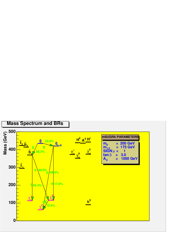
Figure 1: Mass spectrum and decay modes for the chosen mSUGRA point

The signal production cross section times branching ratios is: $\sigma(\tilde{q}\tilde{g}\rightarrow q+2b+2\ell+2\tilde{\chi}^{0}_{1})=1.58$pb. It should be noted that for this point the total SUSY inclusive cross section is O(200pb) and that it may produce a significant ”SUSY background” that has to be accounted for on top of the usual Standard Model background.

3 EVENT SELECTION

3.1 Online Selection

The level 3 trigger, also known as High Level Trigger[275], was crudely simulated by updating the ATLFAST trigger cuts. Fig.2 shows the distribution of the online selected events as a function of the trigger menus.

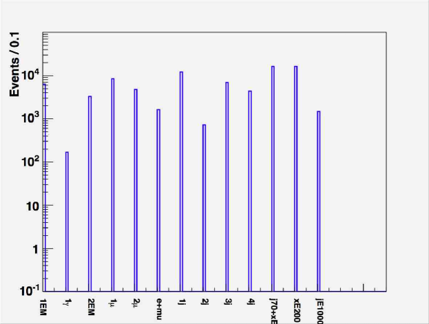
Figure 2: The different trigger menus used for the online selection

We can see that about the third of the selected events pass a menu of the 3 following categories: the leptons menus, the jets menus and the $\hbox to0.0pt{\kern 2.5pt/\hss}E_{T}$ menus. The overall efficiency of the signal obtained with an ”or” of these trigger menus is 99.7$\%$.

3.2 Preselection

The preselection aims at rejecting most of the QCD background whilst keeping the highest signal efficiency. The cuts applied at this level define the studied topology. They are obviously defined as additional requirements with respect to the online selection and defined as follows:

$$\begin{cases}\rm exactly\ 2\ isolated\ leptons\ (with\ opposite\ signs\ and\ same\ flavor)\cr\rm p_{T}(e^{\pm})>5\ {\rm GeV},p_{T}(\mu^{\pm})>6\ {\rm GeV}\cr|\eta(\ell^{\pm})|<2.5\cr{\rm at\ least\ 3\ jets}\cr p_{T}(jets)>10\ {\rm GeV}\cr|\eta(jets)|<5.0\cr\hbox to0.0pt{\kern 2.5pt/\hss}E_{T}>100\ {\rm GeV}\end{cases}$$

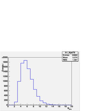
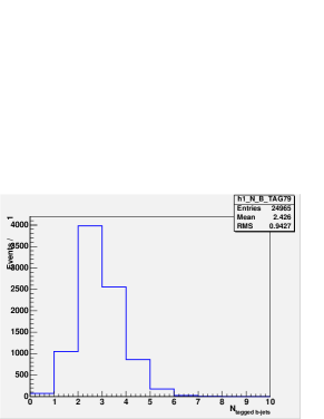
Figure 3: Untagged (left) and b-tagged (right) jet mutiplicities after the preselection

Fig.3 shows the total number of reconstructed jets (left) as well as the number of b-tagged jets. For the later an efficiency of 60$\%$ was used for jet actually coming from a b quark fragmentation whereas a rejection factor of about 7 and 100 was used for jet from c quarks and light flavor quarks respectively. These values, as well as correction factors depending on the jet $p_{T}$ are taken from the ATLFAST-B program. The signal efficiency after applying these preselection cuts is: $\epsilon(\rm signal)=49.3\%$.

3.3 Double-Tag Analysis

Though it’s in principle possible to perform this signal search requiring only 1 b-tagged jet in the events, we directly required 2 b-tagged jets in order to facilitate the jets combinatorics between the squark and the gluino hemispheres. Therefore we used the simple strategy of assigning to the gluino hemisphere both the dilepton and the 2 leading b-tagged jets. The leading non b-tagged jet was systematically assigned to the squark hemisphere. This leads us to adopt the following additional cuts with respect to the preselection requirements:

$$\begin{cases}\rm at\ least\ 2\ b-tagged\ jets\cr\rm p_{T}(jet_{1},jet_{2},jet_{3})>50,30,20\ GeV\end{cases}$$

The signal efficiency after applying these final cuts is: $\epsilon(\rm signal)=14.7\%$. So for an integrated luminosity of $\int\cal L\rm dt=10\ fb^{-1}$ one still expects more than 2400 signal events.

4 MASS RECONSTRUCTION

4.1 $\tilde{\chi}^{0}_{2}$ Reconstruction

We reconstructed the dilepton invariant mass and could determine this way the kinematical edge which is an estimator of the $m(\tilde{\chi}^{0}_{2})-m(\tilde{\chi}^{0}_{1})$ mass difference. This is displayed at different levels of the event selection on Fig.4.

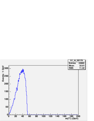
Figure 4: $\tilde{\chi}^{0}_{2}$ mass reconstruction

We can see that the bad combinations that appear beyong the kinematical edge are rare after the preselection and even more so after the final selection, though no special treatment was applied to remove the leptons that come from a B or C hadron semi-leptonic decay.

One notes that the kinematical edge points near the expected value of 54 GeV for our signal point. No fits and no uncertainty estimates on the actual value derived from this histogram are made so far.

4.2 $\tilde{b}_{1}$ Reconstruction

We reconstructed the $m(\tilde{b}_{1})-m(\tilde{\chi}^{0}_{1})$ mass difference by calculating the 3-body invariant mass of the dilepton and one of the 2 leading b-tagged jets. There are obviously wrong combinations that enter the distribution in Fig.5. But we are exclusively interested the largest value of the 2 combinations where we indeed see a kinematical edge.

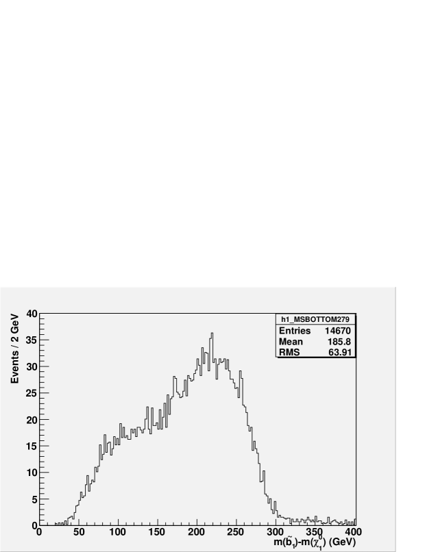
Figure 5: $\tilde{b}_{1}$ mass reconstruction

Again, one notes that the edge points near the expected value of 309 GeV for our signal point.

4.3 $\tilde{g}$ Reconstruction

Finally we reconstruct the $m(\tilde{g})-m(\tilde{\chi}^{0}_{1})$ mass difference by calculating the 4-body invariant mass obtained with the dilepton and the 2 leading b-tagged jets.

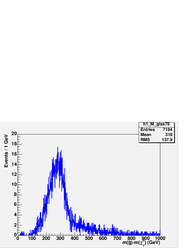
Figure 6: $\tilde{g}$ mass reconstruction

There one sees that the edge points slightly higher than the expected value of 360 GeV for our signal point.

5 CONCLUSIONS AND PROSPECTS

5.1 Conclusions

We have shown that the $pp\rightarrow\tilde{q}+\tilde{g}\rightarrow q+\tilde{b}_{1}\bar{b}\rightarrow q+\tilde{\chi}^{0}_{1}+b\bar{b}\tilde{\chi}^{0}_{2}\rightarrow q+b\bar{b}+\ell^{+}\ell^{-}+2\tilde{\chi}^{0}_{1}$ is a quite interesting process to search for and to study at the LHC. By looking at the signal alone, it seems feasible to reconstruct the following mass differences using the classical kinematical edges: $m(\tilde{\chi}^{0}_{2})-m(\tilde{\chi}^{0}_{1})$, $m(\tilde{b}_{1})-m(\tilde{\chi}^{0}_{1})$ and $m(\tilde{g})-m(\tilde{\chi}^{0}_{1})$.

5.2 Prospects

This study will be continued with the addition of both the Standard Model and the SUSY backgrounds. First of all the signal significance will be calculated with the current final cuts and the cuts will be adjusted if necessary. The effect of the background processes on the sparticle mass reconstruction will be estimated.

Acknowledgements

We would like to thank the IPN Lyon and the IN2P3 for their financial support.

Part 13 Sensitivity of the LHC to CP violating Higgs bosons

R.M. Godbole, D.J. Miller, S. Moretti and M.M. Muhlleitner

1 INTRODUCTION

Whereas in the Standard Model (SM) CP violating effects are tiny, extensions of the SM, such as 2-Higgs doublet models, exhibit new sources of CP violation which can lead to sizeable effects in the Higgs sector [276, 97, 277]. In minimal supersymmetric theories, which are specific realizations of 2-Higgs doublet models, two complex Higgs doublets have to be introduced to remove anomalies. After three of the Higgs doublet components have been absorbed to provide masses to the electroweak gauge bosons, the remaining five components give rise to a quintet of physical Higgs boson states. In a CP-conserving theory, besides two charged Higgs bosons, there are two CP-even neutral Higgs fields and one CP-odd neutral state. In case of CP violation in the Higgs sector the neutral Higgs bosons mix to give three Higgs states with indefinite CP quantum numbers. While the prospects of establishing the CP quantum number of a spin 0 state at the upcoming colliders are quite good, determination of the CP mixing, should the state have an indefinite CP quantum number, is not very easy (See [278] for example for a recent summary).

In this note we present observables which are sensitive to CP violation in order to investigate the sensitivity of the LHC to CP violation in the Higgs sector. We then show preliminary results and give an outlook of the ongoing project.

2 THE DISTRIBUTIONS SENSITIVE TO CP VIOLATION

We exploit the Higgs decays to $Z$ boson pairs to determine spin and parity of the Higgs boson. The Higgs boson is produced in gluon fusion at the LHC, and the $Z$ bosons subsequently decay into fermion pairs

$$gg\to H\to ZZ\to(f_{1}\bar{f_{1}})(f_{2}\bar{f}_{2})$$ (1)

This process includes clean $\mu^{+}\mu^{-}$ and $e^{+}e^{-}$ decay channels for isolating the signal from the background and allowing a complete reconstruction of the kinematical configuration with good precision [279, 280, 281].

In Ref.[282] it has been shown that a model-independent analysis can be performed if supplemented by additional angular correlation effects in gluon gluon fusion. To this end helicity methods have been applied to generalize the Higgs coupling to $Z$ bosons to arbitrary spin and parity. The most general vertex for a spin-0 Higgs boson in a CP non conserving theory can then be written as

$$\frac{igM_{Z}}{\cos\theta_{W}}[\,ag_{\mu\nu}+\frac{b}{M_{Z}^{2}}p_{\mu}p_{\nu}+i\frac{c}{M_{Z}^{2}}\epsilon_{\mu\nu\alpha\beta}p^{\alpha}k^{\beta}\,]$$ (2)

with $p=p_{Z_{1}}+p_{Z_{2}}$, $k=p_{Z_{1}}-p_{Z_{2}}$, $p_{Z_{1}}$ and $p_{Z_{2}}$ being the four-momenta of the two $Z$ bosons, respectively, and $\theta_{W}$ denoting the electroweak mixing angle. The coefficients $a,b,c$ depend on the theory, where $c\neq 0$ is indicative of CP violation. The tree level Standard Model case is recovered for $a=1$ and $b=c=0$. Note that this choice of vertex is gauge invariant for this process. Any gauge dependence in the $Z$ propagators is trivially cancelled when contracted with the conserved lepton currents.

In the following we present the invariant mass distribution and the azimuthal angular distribution of the Higgs decay width into two $Z$ bosons. The azimuthal angle $\phi$ is defined as the angle between the planes of the fermion pairs stemming from the $Z$ boson decays, cf. Fig. 1.

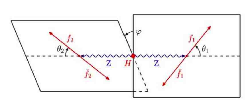
Figure 1: The definition of the polar angles ${\theta_{i}}$ ($i=1,2$) and the azimuthal angle $\varphi$ for the sequential decay $H\rightarrow Z^{(*)}Z\rightarrow(f_{1}\bar{f}_{1})(f_{2}\bar{f}_{2})$ in the rest frame of the Higgs particle.

Fig. 2 left shows the invariant mass distribution for a Higgs boson of 150 GeV, decaying into a pair of virtual and real $Z$ bosons. We compare the distribution for a certain choice of the parameters $a,b,c$ in the coupling given in Eq. (2) to the SM result. Fig. 2 right presents the azimuthal angular distribution for a Higgs particle of 280 GeV decaying in pair of real $Z$ bosons, again compared to the Standard Model. As can be inferred from the figures, the distributions show a distinct behaviour for different models, encouraging further investigation of the angular observables with respect to the sensitivity of the LHC to CP violation in the Higgs sector.

     

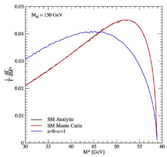
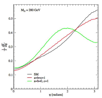
Figure 2: The differential invariant mass distribution [left] and the azimuthal angular distribution [right] for $M_{H}=150$ GeV and $M_{H}=280$ GeV, respectively. The parameterization corresponds to the parameterization of the $HZZ$ vertex given in Eq. (2).

3 SENSITIVITY OF THE LHC TO CP VIOLATION

In order to get a first estimate of the sensitivity of the LHC to CP violation in the Higgs sector the cross section of the process given in

 

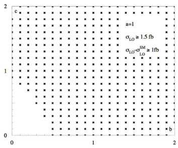
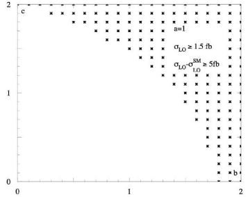
Figure 3: The sensitivity of the LHC to CP violation represented in the [$b,c$] plane for $a=1$, $M_{H}=150$ GeV for two different sensitivity criteria.

Eq. (1) has been calculated for a Higgs boson mass of 150 GeV as a function of the parameters $b$ and $c$. The parameter $a$ has been chosen equal to the SM value, i.e. $a=1$. For simplicity we choose the Higgs coupling to the gluons to be the same as in the SM. The Higgs production cross section in gluon fusion has been calculated with the program HIGLU [283] which includes the QCD corrections at next-to-leading order. Again for simplicity, in the calculation of the branching ratio of the Higgs boson, we adopt the SM $HWW$ coupling and only modify the $HZZ$ coupling. Furthermore, it has been assumed that the cuts applied to reduce the background alter the cross section in the same way as in the SM case, i.e. by about a factor 10 for an integrated luminosity of 100 fb^-1 [279]. Since the ATLAS study, where this number has been taken from, is done for a LO gluon fusion cross section, the following results are presented for the LO production for reasons of consistency. NLO corrections would alter the production section by about a factor 2 before cuts. In Fig. 3 we present the scatter plots in be $[b,c]$ plane representing the points which fulfill the sensitivity criteria we adopt. In order to have large enough significances (at least $\makebox[0.0pt][l]{\raisebox{2.0pt}{$\scriptstyle{>}$}}\raisebox{-2.0pt}{$\scriptstyle{\sim}$}5$) the total cross section is required to be larger than 1.5 fb. Furthermore, the difference between the cross section including the general CP violating $HZZ$ coupling should differ from the SM cross section by more than 1(5) fb. Our sensitivity criteria, for $gg\to H\to Z^{*}Z^{*}\to(l^{+}l^{-})(l^{+}l^{-})$ , are

$$\sigma^{b,c\neq 0}>1.5\;\mbox{fb}\quad\quad\mbox{(}l=e,\mu\mbox{)}$$ (3)

$$|\sigma^{b,c\neq 0}-\sigma^{\mbox{\small SM}}|>1(5)\;\mbox{fb}$$

Fig. 3 shows the sensitivity areas in the $[b,c]$ plane according to the criteria Eq. (3) in case the difference to the SM result exceeds 1 fb (left) and 5 fb (right). In the former case the sensitivity area is almost covered by the LHC.

4 OUTLOOK

In the next step we will confront our results obtained for the LHC sensitivity with proposed CP violating models in the literature and we will refine the experimental side of the analysis. We will furthermore investigate to which extent the LHC will be sensitive to CP violation in the various distributions presented in section 2. The analysis will as well be extended to the most general case, i.e. to spin 1 and spin 2 particle couplings to $ZZ$ in order to be as model-independent as possible. The resulting program PHIZZ will be made available to the experimental community for more detailed studies.

Part 14 Testing the scalar mass universality of mSUGRA at the LHC

S. Kraml, R. Lafaye, T. Plehn and D. Zerwas

If supersymmetry is realised in nature, sparticle masses will be measured from measurements of kinematic endpoints [167, 284] in cascade decays like $\tilde{q}_{L}\to q\tilde{\chi}^{0}_{2}\to ql^{\pm}\tilde{l}_{R}^{\mp}\to ql^{\pm}l^{\mp}\tilde{\chi}^{0}_{1}$ at the LHC. The optimal next step would then be to extract the SUSY breaking parameters at the electroweak scale in a global fit and extrapolate them to the GUT scale [285, 53] to test their high-scale boundary conditions. A complete MSSM fit may, however, have too many parameters compared to the number of observables available at the LHC. This has been shown recently using new fitting tools such as Fittino [54, 53] and SFitter [56]. The alternative procedures will then be to determine the underlying parameters either by fixing a sufficient number of parameters (those the least sensitive to the avaialable measurements) to a defined value or in top-down fits of particular models of SUSY breaking. Such top-down fits, see e.g. [284], are in fact quite popular in benchmark studies within the minimal supergravity (mSUGRA) model, in which the SUSY-breaking gaugino, scalar and trilinear parameters $m_{1/2}$, $m_{0}$ and $A_{0}$, respectively, each obey universal boundary conditions at the GUT scale,

However, as we discuss in this contribution, care has to be taken not to draw too strong conclusions from just a mSUGRA fit. As a matter of fact, the determination of the common scalar mass, $m_{0}$, is dominated by the precise measurement of the endpoint of the $l^{\pm}l^{\mp}$ invariant mass $m_{ll}^{max}$ —in other words by the $\tilde{\chi}^{0}_{1}$, $\tilde{\chi}^{0}_{2}$ and $\tilde{l}_{R}$ mass differences. Kinematic endpoints involving jets, which give the squark and gluino masses, are measured about an order of magnitude less precisely than $m_{ll}^{max}$. Moreover, in the renormalization group running, the squark mass parameters are driven by $m_{1/2}$ with a large coefficient and are hence much less sensitive to $m_{0}$ than the slepton masses:

$$m_{\tilde{L}}^{2}\sim m_{0}^{2}+0.5\,m_{1/2}^{2}\,, m_{\tilde{E}}^{2}\sim m_{0}^{2}+0.15\,m_{1/2}^{2}\,,$$ (1)

$$m_{\tilde{Q}}^{2}\sim m_{0}^{2}+6.3\,m_{1/2}^{2}\,, m_{\tilde{U}\!,\tilde{D}}^{2}\sim m_{0}^{2}+5.8\,m_{1/2}^{2}\,.$$ (2)

Additionally the error on $m_{0}$ is proportional to the product of the error on sfermion mass and the sfermion mass itself. Thus for a squark mass typically three times as large as a slepton mass, the relative experimental error on the squark mass measurement must be an order of magnitude more precise than the measurement of the slepton mass to obtain the same sensitivity, which is difficult to achieve. For these reasons, measurements of squarks have little influence on the fit of a universal $m_{0}$.

While the assumption of a universal $m_{0}$ simplifies the model a lot, there is no strong theoretical basis for this. When embedded in a higher gauge group, sparticles which come in the same multiplet have equal masses. This is for example the case for squarks and sleptons in SU(5) or SO(10) GUTs. Non-universal scalar masses are also heavily constrained by flavour-changing neutral currents (FCNC), at least for the first and second generation. However, there may be non-universal D-terms and/or GUT-scale threshold corrections, and the FCNC constraints are much less severe for the third generation. Last but not least, there is no sound theoretical argument whatsoever for the universality of the mass-squared terms, $m_{H_{1,2}}^{2}$, of the Higgs fields. (If it is given up, $\mu$ and $m_{A}$ become free parameters of the model.) For these reasons, and because of it’s important phenomenological implications, the assumption of scalar-mass universality should be treated with caution.

In this contribution, we study the implications of relaxing the scalar-mass universality of mSUGRA in the top-down parameter determination. To this aim, we assume the perspective LHC edge measurements at SPS1a according to [75]. In general, several of the LHC measurements of SPS1a with an integrated luminsoity of 300 fb^-1 are dominated by the systematic error on the knowledge of the energy scale, which is 1% for jets and 0.1% for leptons (electrons and muons). For the light Higgs mass, $m_{h^{0}}$, we assume an experimental error of 250 MeV and a theoretical error of 3 GeV [156]. We then use SFITTER [56, 55] to determine the parameters for non-universal SUGRA scenarios. The results are summarized in Table 1. First, as a reminder, case A shows the results of a strict mSUGRA fit [55], which leads to a ${\cal O}(1\%)$ accuracy on $m_{0}$, $m_{1/2}$ and $\tan\beta$, and $\sim 20$ GeV accuracy on $A_{0}$. Note that as poited out in [55] the fit to the edge variables gives a much better result than the fit to the extracted SUSY masses. Next, for case B, we have relaxed the universality between slepton, squark and Higgs mass parameters, treating $m_{0}(\tilde{l})$, $m_{0}(\tilde{q})$ and $m_{H}^{2}=m_{H_{1}}^{2}=m_{H_{2}}^{2}$ as independent parameters. As expected, the scalar-mass parameter of the squarks, $m_{0}(\tilde{q})$, turns out to be an order of magnitude less well dertermined than that of the sleptons, $m_{0}(\tilde{l})$. The Higgs mass parameters have a very large $\sim 100\%$ errror in this case. The precision on $\tan\beta$ and $A_{0}$ also degrades, for $\tan\beta$ by a factor of 1.6 and for $A_{0}$ by a factor of 2.6 (from 21 GeV to 54 GeV). Finally, in case C we have assumed universal scalar masses for sleptons and squarks of the first two generations ($\tilde{l},\tilde{q}$), but treated those of the third generation and of the Higgs fields as free parameters. The resulting errors on $m_{0}(\tilde{t},\tilde{b})$ and $m_{0}(\tilde{l},\tilde{q})$ are more or less similar to case B, but that on $m_{H}^{2}$ becomes almost 200% and $m_{0}(\tilde{\tau})$, relying almost only on the $\tau\tau$ invariant mass edge measurement, remains undetermined. Also the error on $A_{0}$ increases to 75 GeV.

Parameter	value	(A)	(B)	(C)	(D)
$\tan\beta$	10	1.5	2.4	2.4	2.1
$m_{1/2}$	250	1.1	1.6	1.3	1.3
$m_{0}$	100	1.4	–	–	–
$m_{0}(\tilde{l})$	100	–	1.4	–	–
$m_{0}(\tilde{q})$	100	–	16	–	–
$m_{0}(\tilde{l},\tilde{q})$	100	–	–	1.5	1.5
$m_{0}(\tilde{t},\tilde{b})$	100	–	–	20	17
$m_{0}(\tilde{\tau})$	100	–	–	200	200
$m_{H}^{2}$	10000	–	11000	20000	15000
$A_{0}$	$-100$	21	54	75	63

Table 1: (A) Parameter errors obtained with a fit of mSUGRA to LHC edge and threshold measurements at SPS1a. (B) Same as A but relaxing the universality between $\tilde{l}$, $\tilde{q}$ and Higgs mass terms. (C) Same as A but relaxing the universality between the 1st/2nd and the 3rd generation of squarks and sleptons, and the Higgs mass terms. (D) Same as D adding $m_{A}$ measurement (400 GeV) with a 40 GeV uncertainty.

We have also studied the influence of particular measurements on the fit. The measurement of the sbottom masses, for instance, is of course crucial for the determination of $m_{0}(\tilde{t},\tilde{b})$. In addition, it also has an important impact on the determination of $\tan\beta$ and $A_{0}$: without the sbottom measurement, the error on $\tan\beta$ increases by about a factor of 2 and that on $A_{0}$ by about a factor of 4 in cases B and C. The influence of $m_{h}$ is small in these cases because of its 3 GeV theoretical uncertainty. The pseudoscalar mass $m_{A}$, on the other hand, would have an important influence. A measurement of $m_{A}$ at the level of 10% would mainly improve the error on $\tan\beta$. This is shown as case D in Table 1. In order to determine $m_{H}^{2}$, one would need to obtain a better uncertainty on the Higgs masses and to know the $\mu$ parameter in addition.

In summary, at SPS1a, with the anticipated measurements at the LHC with 300 fb^-1, the universality of the scalar mass parameters of squarks and sleptons at the GUT scale can be tested to the level of 10%–20%. Moreover, with the standard measurements, there is no sensitivity to the GUT-scale values of the scalar mass parameters of the Higgs fields. The scalar-mass parameters of the squark and Higgs sectors also have an important influence on the fit results of $\tan\beta$ and $A_{0}$.

Acknowledgements

We thank the organisers and conveners of the Les Houches 2005 workshop for creating a very pleasant and inspiring working atmosphere. S.K. is supported by an APART (Austrian Programme of Advanced Research and Technology) grant of the Austrian Academy of Sciences. She also acknowledges financial support of CERN for the participation at this workshop.

blabla

TOOLS

Part 15 A repository for beyond-the-Standard-Model tools

P. Skands, P. Richardson, B. C. Allanach, H. Baer, G. Bélanger, M. El Kacimi, U. Ellwanger, A. Freitas, N. Ghodbane, D. Goujdami, T. Hahn, S. Heinemeyer, J.-L. Kneur, G. Landsberg, J. S. Lee, M. Mühlleitner, T. Ohl, E. Perez, M. Peskin, A. Pilaftsis, T. Plehn, W. Porod, H. Przysiezniak, A. Pukhov, D. Rainwater, J. Reuter, S. Schumann, S. Sherstnev, M. Spira and S. Tsuno

1 INTRODUCTION

The physics programme at present and future colliders is aimed at a truly comprehensive exploration of the TeV scale. On the theoretical side, recent years have seen the emergence of an impressive variety of proposals for what physics may be uncovered by these machines in just a few years. The ideas range from hypotheses of new fundamental matter (e.g. right-handed neutrinos) or forces ($\mathrm{Z}^{\prime}$ models), to new space-time symmetries (supersymmetry), or even new spatial dimensions — at times with singularly spectacular consequences, such as the possible production of microscopic black holes.

In the wake of many of these proposals, developments of computerised calculations of mass spectra, couplings, and experimental observables, have taken place. For others, such tools are yet to be created. Let it be stressed that this is not a point of only theoretical or phenomenological interest. Experiments and analyses are not constructed purely with mechanical tools. Theoretical predictions, for expected signal strengths as well as background levels, constitute a crucial part of the optimisation of both detectors, triggers, and analysis strategies. It is therefore essential to have access to tools for calculating observables for as wide a range of phenomenological signatures as possible.

The present brief overview and associated web repository aims to assess the present situation and facilitate the information gathering process for people wishing to perform phenomenological calculations in scenarios of physics beyond the Standard Model. We hope this may serve also to stimulate further work in the field. In Section 2, we first present a brief index of codes organised by physics topic. Next, in Section 3, a full, alphabetical overview is given, describing the contents of the repository at the time of writing. Other recent overviews of BSM-related physics tools can be found in [286, 287, 288, 289].

2 TOOLS BY PHYSICS TOPIC

This section is merely intended as an index, useful for finding out which tools exist for a given physics scenario. The main repository is then described in alphabetical order in the next section.

Supersymmetry

• CalcHEP: MSSM tree-level matrix element generator. Phase space integration and event generation. Extensions possible.

• CompHEP: MSSM tree-level matrix element generator. Phase space integration and event generation. Extensions possible.

• CPsuperH: Higgs phenomenology in the MSSM with explict CP Violation.

• FeynHiggs: MSSM Higgs sector including explicit CP-violation (masses, couplings, branching ratios, and cross sections).

• Herwig: Event generator for the MSSM (with and without RPV). Interface to Isajet.

• ILCslepton: NLO cross-sections for slepton production in $\mathrm{e}^{+}\mathrm{e}^{-}$ and $\mathrm{e}^{-}\mathrm{e}^{-}$ collisions.

• HDecay: MSSM Higgs decay widths including loop effects.

• Isajet: MSSM event generator. MSSM mass and coupling spectrum, decay widths. Checks against experimental constraints.

• micrOMEGAs: MSSM (work on CPV in progress) and NMSSM dark matter relic density.

• NMHDecay: NMSSM mass spectrum plus couplings and decay widths of all Higgs bosons. Checks against experimental constraints.

• O’Mega: MSSM tree-level matrix element generator. Extensions possible.

• Prospino: SUSY-NLO cross sections at hadron colliders.

• Pythia: MSSM event generator. RPV decays. Extensions to R-hadrons and NMSSM available.

• SDecay: MSSM decay widths including loop effects.

• Sherpa: MSSM event generator.

• SoftSusy: MSSM mass and coupling spectrum.

• SPheno: MSSM mass and coupling spectrum, decay widths, and $\mathrm{e}^{+}\mathrm{e}^{-}$ cross sections.

• SuSpect: MSSM mass and coupling spectrum.

• SUSY-MadGraph: MSSM Matrix Elements.

• Susygen3: MSSM event generator (with and without RPV).

Extra Dimensions

• Charybdis: Black hole production in hadron-hadron collisions.

• Herwig: Resonant graviton production in hadron-hadron collisions.

• micrOMEGAs: Dark matter relic density. UED and warped extra dimensions being implemented.

• Pandora/Pandora-Pythia: ADD extra dimensions. Work in progress: UED.

• Pythia: RS graviton excitations.

• Pythia_UED: Universal Extra Dimensions.

• Sherpa: ADD extra dimensions.

• TrueNoir: Black hole production.

Extra Gauge Bosons, $\mathrm{Z}^{\prime}/\mathrm{W}^{\prime}$ models.

• Pandora/Pandora-Pythia: $\mathrm{Z}^{\prime}$ models.

• Pythia: $\mathrm{Z}^{\prime}$ and $\mathrm{W}^{\prime}$ models.

Other Exotics

• O’Mega: Anomalous triple and quartic gauge couplings. Extensions possible.

• Gr@ppa.Leptoquark: Leptoquark event generator for $\mathrm{p}\mathrm{p}$ and $\mathrm{p}\bar{\mathrm{p}}$ collisions.

• Pythia: Technicolor, doubly charged Higgs bosons, excited fermions, anomalous couplings, leptoquarks, fourth generation fermions.

3 TOOLS BY ALPHABET

We here give a detailed alphabetical list of the tools present in the repository at the time these proceedings went to press. Note that the preceding section contains a useful list of tools by topic, i.e. which tools are relevant for extra dimensions, which ones for Z’ etc.

CalcHEP

Contact Person: A. Pukhov, pukhov@lapp.in2p3.fr

Web Page: http://theory.sinp.msu.ru/$\sim$pukhov/calchep.html

CalcHEP is a program for symbolic calculation of matrix elements and generation of C-codes for subsequent numerical calculations. The model has to be defined in tems of lists of variables, constraints, particles and list of vertices. Various BSM can be implemented and investigated. In partiqular CalcHEP links to SuSpect, Isajet, SoftSusy, and SPheno for MSSM. It also contains a Monte Carlo generator for unweighted events and a simple program which passes these events to Pythia. CalcHEP is a menu driven system with context help facility and is accompanied by a manual. At the same time CalcHEP can be used in the non-interactive regime as a generator of matrix elements for other programs. In this mode it is implemented in micrOMEGAs for automatic generation of matrix elements of annihilation and co-annihilation of super-particles. Restrictions: tree level matrix elements, not more than 6 particles in initial/final states. The last restriction is caused by modern computer facilities and by the implemented method of calculation (squared amplitudes). But for calculation of separate diagrams it was successfuly used for 2$\to$5 and 2$\to$6 processes.

Charybdis

Contact Person: P. Richardson, Peter.Richardson@durham.ac.uk

Web Page: www.ippp.dur.ac.uk/montecarlo/leshouches/generators/charybdis/

Charybdis simulates black hole production in hadron-hadron collisions using a geometric approximation for the cross section together with Hawking evaporation of the black hole using the correct grey-body factors. It is described in more detail in [290].

CompHEP

Contact Person: Sasha Sherstnev, sherstnv@theory.sinp.msu.ru

Web Page: http://theory.sinp.msu.ru/comphep

The CompHEP package was created for calculation of multiparticle final states in collision and decay processes. The main idea in CompHEP was to enable one to go directly from the lagrangian to the cross sections and distributions effectively, with the high level of automation. The officially supported models are SM (in two gauges), unconstrained MSSM (in two gauges), MSSM with SUGRA and Gauge-Mediated SUSY breacking machanisms. The special program LanHEP allows new BSM models to be implemented to CompHEP.

CPsuperH

Contact Persons: J. S. Lee, jslee@hep.man.ac.uk
A. Pilaftsis, pilaftsi@mail.cern.ch

Web Page: http://www.hep.man.ac.uk/u/jslee/CPsuperH.html

CPsuperH [97] is a newly-developed computational package that calculates the mass spectrum, couplings and branching ratios of the neutral and charged Higgs bosons in the Minimal Supersymmetric Standard Model with explicit CP violation [291, 292, 293, 294, 93]. The program is based on recent renormalization-group-improved diagrammatic calculations that include dominant higher-order logarithmic and threshold corrections, b-quark Yukawa-coupling resummation effects and Higgs-boson pole-mass shifts [295, 296, 297, 298, 299].

The code CPsuperH is self-contained (with all subroutines included), is easy and fast to run, and is organized to allow further theoretical developments to be easily implemented. The fact that the masses and couplings of the charged and neutral Higgs bosons are computed at a similar high-precision level makes it an attractive tool for Tevatron, LHC and LC studies, also in the CP-conserving case.

FeynHiggs

Contact Person: T. Hahn, hahn@mppmu.mpg.de
S. Heinemeyer, Sven.Heinemeyer@cern.ch

Web Page: http://www.feynhiggs.de

FeynHiggs is a program for computing MSSM Higgs-boson masses and related observables, such as mixing angles, branching ratios, couplings and production cross sections, including state-of-the-art higher-order contributions (also for the case of explicit CP-violation). The centerpiece is a Fortran library for use with Fortran and C/C++. Alternatively, FeynHiggs has a command-line, Mathematica, and Web interface. The command-line interface can process, besides its native format, files in SUSY Les Houches Accord format. FeynHiggs is an open-source program and easy to install. A web-based interface is available at www.feynhiggs.de/fhucc . For further information, see also [300, 155, 277, 156, 74].

GR@PPA.Leptoquark

Contact Person: S. Tsuno, Soushi.Tsuno@cern.ch

Web Page: http://atlas.kek.jp/physics/nlo-wg/index.html

GR@PPA event generator for Leptoquark model. The code generates unweighted events for scalar or vector type Leptoquark models. The Leptoquarks are generated, and decayed into quark and lepton(neutrino) so that the decay properties of the final particles are correctly handled. In the vector Leptoquark production, two anomalous couplings are included in the interaction vertices. The decay mode depends on the model induced in the unified theory. The program thus keeps flexibility for the Leptoquark decay. The details description can be found on the web page, where also the model file which contains the Leptoquark interaction for the Grace system is available.

HDecay

Contact Person: M. Spira, Michael.Spira@psi.ch

Web Page: http://people.web.psi.ch/spira/hdecay/

HDecay [301] calculates the branching ratios and total widths of SM and MSSM Higgs bosons.

Herwig

Contact Person: P. Richardson, Peter.Richardson@durham.ac.uk

Web Page: http://hepwww.rl.ac.uk/theory/seymour/herwig/

Herwig [11] is a general purpose event generator for the simulation of Hadron Emission Reactions With Interfering Gluons. The main concentration is on the simulation of the Standard Model although SUSY (with and without RPV [302]) is implemented together with resonant gravition production in hadron-hadron collisions.

ILCslepton

Contact Person: A. Freitas, afreitas@physik.unizh.ch

Web Page: http://theory.fnal.gov/people/freitas/

The programs calculate the complete electroweak one-loop corrections to slepton production in $\mathrm{e}^{+}\mathrm{e}^{-}$ and $\mathrm{e}^{-}\mathrm{e}^{-}$ collisions (i.e. at ILC). Besides the virtual loop corrections, real photon radiation is included in order to provide a finite and well-defined result. For the sake of consistent renormalization, the programs take the MSSM soft breaking parameters at an arbritary scale as input; it is not possible to use masses and mixing angles as input parameters. The available codes allow the computation of the total and angular differential cross-sections for selectron, smuon and sneutrino production. For more information, see [303, 304].

Isajet

Contact Person: H. Baer, baer@hep.fsu.edu

Web Page: http://www.phy.bnl.gov/$\sim$isajet/

Simulates $\mathrm{p}\mathrm{p}$, $\bar{\mathrm{p}}\mathrm{p}$, and $\mathrm{e}^{+}\mathrm{e}^{-}$ interactions at high energies. Calculates SUSY and Higgs spectrum along with SUSY and Higgs 2 and 3 body decay branching fractions. Evaluates neutralino relic density, neutralino-nucleon scattering cross sections, $\mathrm{Br}(\mathrm{b}\to\mathrm{s}\gamma)$, $(g-2)_{\mu}$, $\mathrm{Br}(\mathrm{B}_{\mathrm{s}}->\mu^{+}\mu^{-})$.

micrOMEGAs

Contact Persons: G. Bélanger, F. Boudjema, A. Pukhov, A. Semenov, micro.omegas@lapp.in2p3.fr

Web Page: http://lappweb.in2p3.fr/lapth/micromegas/index.html

micrOMEGAs is a code that calculates the relic density of the dark matter in supersymmetry. All annihilation and coannihilation processes are included. The cross-sections, extracted from CalcHEP, are calculated exactly using loop-corrected masses and mixings as specified in the SUSY Les Houches Accord. Relativistic formulae for the thermal average are used and care is taken to handle poles and thresholds by adopting specific integration routines. In the MSSM, the input parameters can be either the soft SUSY parameters or the parameters of a SUGRA model specified at the GUT scale. In the latter case, a link with Suspect, Softsusy, Spheno and Isajet allows to calculate the supersymmetric spectrum, Higgs masses, as well as mixing matrices. Higher-order corrections to Higgs couplings to quark pairs including QCD as well as some SUSY corrections are implemented. Cross-sections for any 2$\to$2 process as well as partial decay widths for two-body final states are provided. Cross-sections for neutralino annihilation at v$\sim$0, relevant for indirect detection of neutralinos, are automatically computed. In the MSSM, routines calculating $(g-2)_{\mu}$, $\mathrm{Br}(\mathrm{b}\to\mathrm{s}\gamma)$, $\mathrm{Br}(\mathrm{B}_{\mathrm{s}}\to\mu^{+}\mu^{-})$ are also included. micrOMEGAs can be extended to other models by specifying the corresponding model file in the CalcHEP notation.

NMHDecay

Contact Person: U. Ellwanger, ellwanger@th.u-psud.fr

Web Page: http://www.th.u-psud.fr/NMHDECAY/nmhdecay.html

The Fortran code NMHDecay computes the sparticle masses and masses, couplings and decay widths of all Higgs bosons of the NMSSM in terms of its parameters at the electroweak (SUSY breaking) scale: the Yukawa couplings $\lambda$ and $\kappa$, the soft trilinear terms $A_{\lambda}$ and $A_{\kappa}$, and $\tan(\beta)$ and $\mu_{\mathrm{eff}}=\lambda<S>$. The computation of the Higgs spectrum includes the leading two loop terms, electroweak corrections and propagator corrections. Each point in parameter space is checked against negative Higgs bosons searches at LEP, including unconventional channels relevant for the NMSSM. A link to a NMSSM version of MicrOMEGAs allows to compute the dark matter relic density, and a rough (lowest order) calculation of the BR($\mathrm{b}\to\mathrm{s}\gamma$) is perfromed. One version of the program uses generalized SLHA conventions for input and output. For further information, see also [218, 305].

O’Mega

Contact Person: T. Ohl, ohl@physik.uni-wuerzburg.de
J. Reuter, juergen.reuter@desy.de

Web Page: http://theorie.physik.uni-wuerzburg.de/$\sim$ohl/omega/

O’Mega constructs [306] optimally factorized tree-level scattering amplitudes (starting from 2$\to$4 processes, the expressions are much more compact and numerically stable than naive sums of Feynman diagrams). Officially supported models are the Standard Model and the complete MSSM (since version 0.10, of November 2005). Users can add new interactions (e.g. anomalous triple and quartic gauge couplings are part of the distributed version).

Complete automatized event generation for the LHC and the ILC is possible in concert with WHiZard.

Pandora

Contact Person: M. Peskin, mpeskin@slac.stanford.edu

Web Page: http://www-sldnt.slac.stanford.edu/nld/new/
Docs/Generators/PANDORA.htm

Pandora is a parton-level physics simulation for $\mathrm{e}^{+}\mathrm{e}^{-}$ linear colliders, including polarization and beam effects. Pandora comes with an interface, Pandora-Pythia, that hadronizes events with Pythia and decays polarized taus with tauola. The current distribution (Pandora 2.3) includes an implementation of the ADD extra dimension model ($\mathrm{e}^{+}\mathrm{e}^{-}\to\gamma\mathrm{G}$ and virtual graviton exchange in $\mathrm{e}^{+}\mathrm{e}^{-}\to\mathrm{f}\bar{\mathrm{f}}$, $\mathrm{W}^{+}\mathrm{W}^{-}$, $\mathrm{Z}\mathrm{Z}$, $\gamma\gamma$), and a two-parameter $\mathrm{Z}^{\prime}$ model. We are currently working on inclusion of more general $\mathrm{Z}^{\prime}$ models and inclusion of UED production and decay.

Prospino

Contact Person: T. Plehn, tilman.plehn@cern.ch

Web Page: http://pheno.physics.wisc.edu/$\sim$plehn

For most applications the uncertainty in the normalization of Monte Carlos for the production of two supersymmetric particles is large. The reason are large SUSY and SUSY-QCD corrections to the cross section. Prospino2 is the tool you can to use to normalize your total rates. Some distributions are available on request. For detailed information on the production processes included, on papers available for more information, and on downloading and running the code, please see the web pages.

Pythia

Contact Person: P. Skands, skands@fnal.gov

Web Page: http://www.thep.lu.se/$\sim$torbjorn/Pythia.html

In the context of tools for extra dimensions, Pythia contains cross sections for the production of Randall-Sundrum graviton excitations, with the parton showers corrected to RS+jet matrix elements for hard jet radiation [307]. Pythia can also be used for a number of other BSM physics scenarios, such as Technicolor [308], $\mathrm{Z}^{\prime}$/$\mathrm{W}^{\prime}$ [309] (including interference with $\mathrm{Z}/\gamma$ and $\mathrm{W}$ bosons), Left–Right symmetry (Higgs triplets), leptoquarks, compositeness and anomalous couplings (including excited quarks and leptons), and of course a large variety of SUSY signals and scenarios (for $R$-hadrons see [310]; for RPV see [311, 312]; for the NMSSM see [313]). Interfaces to SLHA, Isajet, and FeynHiggs are available. For further information, see the Pythia manual [46], Chapter 8, and the Pythia update notes, both available on the Pythia web page.

Pythia_UED

Contact Person: H. Przysiezniak, helenka@lapp.in2p3.fr
M. El Kacimi D. Goujdami

Web Page: http://wwwlapp.in2p3.fr/$\sim$przys/PythiaUED.html

A generator tool which uses Pythia to produce events in the UED (Universal Extra Dimensions) model of Appelquist, Cheng and Dobrescu [314], with one extra dimension and additional gravity mediated decays [315].

SDecay

Contact Person: M. Mühlleitner, muehl@lapp.in2p3.fr

Web Page: http://lappweb.in2p3.fr/pg-nomin/muehlleitner/SDECAY/

Calculates the 2- and 3-body decays and loop-induced decays of the supersymmetric particles including the QCD corrections to the decays involving coloured particles and the dominant electroweak effects to all decay modes.

Sherpa

Contact Person: S. Schumann, F. Krauss, sherpa@theory.phy.tu-dresden.de

Web Page: http://www.sherpa-mc.de/

Sherpa [316] is a multi-purpose Monte Carlo event generator that is able to simulate high-energetic collisions at lepton and hadron colliders. The physics programme of Sherpa covers: 1) The description of hard processes in the framework of the Standard Model, the Minimal Supersymmetric Standard Model and the ADD model of large extra dimensions using tree level matrix elements provided by its internal matrix element generator Amegic++ [317, 318]. 2) Multiple QCD bremsstrahlung from initial and final state partons. 3) The consistent merging of matrix elements and parton showers according to the CKKW prescription. 4) Jet fragmentation and hadronisation provided by an interface to Pythia. 5) The inclusion of hard underlying events.

Softsusy

Contact Person: B. C. Allanach, B.C.Allanach@damtp.cam.ac.uk

Web Page: http://allanach.home.cern.ch/allanach/softsusy.html

This code provides a SUSY spectrum in the MSSM consistent with input low energy data, and a user supplied high energy constraint (eg minmal SUGRA). It is written in C++ with an emphasis on easy generalisability. Full three-family couplings and renormalisation group equations are employed, as well as one-loop finite corrections a la Bagger, Matchev, Pierce and Zhang. It can produce SUSY Les Houches Accord compliant output, and therefore link to Monte-Carlos (eg Pythia) or programs that calculate decays, (e.g. SDecay). If you use SOFTSUSY to write a paper, please cite [319], which is the SOFTSUSY manual. The version on the electronic hep-ph/ archive will be updated with more recent versions. To run SOFTSUSY, you should only need standard C++ libraries. CERNLIB and NAGLIB are not required. The code has been successfully compiled so far using g++ on SUN, DEC ALPHA and PC systems (linux, sun UNIX and OSF). It is supposed to be standard ANSI compatible C++ (and does not contain any templates).

SPheno

Contact Person: W. Porod, porod@ific.uv.es

Web Page: http://www-theorie.physik.unizh.ch/$\sim$porod/SPheno.html

Solves the SUSY RGEs at the 2-loop level for various high scale models. The obtained parameters are used to calculate the SUSY and Higgs spectrum using the complete 1-loop formulas and in case of the Higgs bosons in addition the 2-loop corrections due to Yukawa interactions. This spectrum is used to calculate SUSY and Higgs decay branching ratios and the production of these particles in e+ e- annihilation.

SuSpect

Contact Person: J.-L. Kneur, jean-loic.kneur@lpta.univ-montp2.fr

Web Page: http://www.lpta.univ- montp2.fr/users/kneur/Suspect/

Calculates the SUSY and Higgs particle spectrum in the general MSSM or more constrained high energy SUSY models. It includes the renormalization group evolution between low and high energy scales at the full two-loop level, and the calculation of the physical particle masses with one-loop radiative corrections (plus leading two-loop corrections for the Higgs bosons). It also provides several optional input/output parameter choices, and some calculations or checks of experimentally or theoretically constrained quantities (e.g. $g_{\mu}-2$, BR($\mathrm{b}\to\mathrm{s}\gamma$), consistent electroweak symmetry breaking, “fine-tuning” information, etc.)

SUSY-MadGraph

Contact Person: T. Plehn, tilman.plehn@cern.ch
D. Rainwater, rain@pas.rochester.edu

Web Page: http://www.pas.rochester.edu/$\sim$rain/smadgraph/smadgraph.html
http://pheno.physics.wisc.edu/$\sim$plehn/smadgraph/smadgraph.html

Generates Fortran code for MSSM matrix elements, which use the HELAS library. MSSM here means R-parity conserving, no additional CP violation, and two Higgs doublets. A corresponding event generator based on MadEvent is under construction.

Susygen3

Contact Person: N. Ghodbane, ghodbane@cern.ch
E. Perez, eperez@hep.saclay.cea.fr

Web Page: http://lyoinfo.in2p3.fr/susygen/susygen3.html

Susygen 3.0 is a Monte Carlo program designed for computing distributions and generating events for MSSM sparticle production in $\mathrm{e}^{+}\mathrm{e}^{-}$ , $\mathrm{e}^{\pm}\mathrm{p}$ and $\mathrm{p}\mathrm{p}$ ($\mathrm{p}\bar{\mathrm{p}}$) collisions. The Supersymmetric (SUSY) mass spectrum may either be supplied by the user, or can alternatively be calculated in different models of SUSY breaking: gravity mediated supersymmetry breaking (SUGRA), and gauge mediated supersymmetry breaking (GMSB). The program incorporates the most important production processes and decay modes, including the full set of R-parity violating decays, and the decays to the gravitino in GMSB models. Single sparticle production via a R-parity violating coupling is also implemented. The hadronisation of the final state is performed via an interface to Pythia.

TrueNoir

Contact Person: G. Landsberg, landsberg@hep.brown.edu

Web Page: http://hep.brown.edu/users/Greg/TrueNoir/index.htm

A Monte Carlo package, TrueNoir, has been developed for simulating production and decay of the black holes at high-energy colliders. This package is a plug-in module for the Pythia [17] Monte Carlo generator. It uses a euristic algorithm and conservation of barion and lepton numbers, as well as the QCD color, to simulate the decay of a black hole in a rapid-decay approximation. While the limitations of this approach are clear, further improvements to this generator are being worked on. In the meantime, it provides a useful qualitative tool to study the detector effects and other aspects of the BH event reconstruction. At the present moment, the generator works for $\mathrm{e}^{+}\mathrm{e}^{-}$ and $\mathrm{p}\bar{\mathrm{p}}$ collisions. The proton-proton collisions are being added; their characteristic is not expected to differ much from those in $\mathrm{p}\bar{\mathrm{p}}$ interactions, so the user is advised to use the $\mathrm{p}\bar{\mathrm{p}}$ mode to generate events at the LHC or VLHC until further notice.

4 OUTLOOK

We present an overview of the tools available in a newly created web repository for Beyond-the-Standard Model physics tools, at the address:
http://www.ippp.dur.ac.uk/montecarlo/BSM/

Most of these tools focus on supersymmetry, but there is a growing number of tools for more ‘exotic’ physics becoming available as well. With a series of at least 3 workshops directly focussing on tools in 2006, and with the Les Houches activities picking up again in 2007, we anticipate that this list will be expanded considerably before the turn-on of the LHC in 2007. For the year 2006, the main tools-oriented workshops are:

1. MC4BSM, Fermilab, Mar 20-21, 2006.
                     http://theory.fnal.gov/mc4bsm/

2. Tools 2006, Annecy, Jun 26-28, 2006.
                     http://lappweb.in2p3.fr/TOOLS2006/

3. MC4LHC, CERN, Jul 17 - 26, 2006.

Acknowledgements

The authors are grateful to the organizers of the “Physics at TeV Colliders” workshop, Les Houches, 2005. Many thanks also to A. de Roeck (CERN) for tireless efforts to encourage this project. Work supported by by Universities Research Association Inc., and the US Department of Energy, contract numbers DE-AC02-76CH03000 and DE–AC02–76SF00515. W.P. is supported by a MCyT Ramon y Cajal contract.

Part 16 Status of the SUSY Les Houches Accord II project

B.C. Allanach, C. Balázs, G. Bélanger, F. Boudjema, D. Choudhury, K. Desch, U. Ellwanger, P. Gambino, R. Godbole, J. Guasch, M. Guchait, S. Heinemeyer, C. Hugonie, T. Hurth^∗, S. Kraml, J. Lykken, M. Mangano, F. Moortgat, S. Moretti, S. Penaranda, W. Porod, A. Pukhov, M. Schumacher, L. Silvestrini, P. Skands, P. Slavich, M. Spira, G. Weiglein and P. Wienemann
^∗ Heisenberg Fellow.

1 INTRODUCTION

Supersymmetric extensions of the Standard Model rank among the most promising and well-explored scenarios for New Physics at the TeV scale. Given the long history of supersymmetry and the number of both theorists and experimentalists working in the field, several different conventions for defining supersymmetric theories have been proposed over the years, many of which have come into widespread use. At present, therefore, there is not one unique definition of supersymmetric theories which prevails. Rather, different conventions are adopted by different groups for different applications. In principle, this is not a problem. As long as everything is clearly and completely defined, a translation can always be made between two sets of conventions, call them A and B.

However, the proliferation of conventions does have some disadvantages. Results obtained by different authors or computer codes are not always directly comparable. Hence, if author/code A wishes to use the results of author/code B in a calculation, a consistency check of all the relevant conventions and any necessary translations must first be made – a tedious and error-prone task.

To deal with this problem, and to create a more transparent situation for non-experts, the original SUSY Les Houches Accord (SLHA1) was proposed [92]. This accord uniquely defines a set of conventions for supersymmetric models together with a common interface between codes. The most essential fact is not what the conventions are in detail (they largely resemble those of [320]), but that they are complete and unambiguous, hence reducing the problem of translating between conventions to a linear, rather than a quadratic, dependence on the number of codes involved. At present, these codes can be categorised roughly as follows (see [321, 322] for a quick review and online repository):

• Spectrum calculators [323, 319, 35, 62], which calculate the supersymmetric mass and coupling spectrum, assuming some (given or derived) SUSY breaking terms and a matching to known data on the Standard Model parameters.

• Observables calculators [162, 324, 300, 325, 6, 326, 218]; packages which calculate one or more of the following: collider production cross sections (cross section calculators), decay partial widths (decay packages), relic dark matter density (dark matter packages), and indirect/precision observables, such as rare decay branching ratios or Higgs/electroweak observables (constraint packages).

• Monte-Carlo event generators [11, 17, 46, 327, 328, 329, 289, 330], which calculate cross sections through explicit statistical simulation of high-energy particle collisions. By including resonance decays, parton showering, hadronisation, and underlying-event effects, fully exclusive final states can be studied, and, for instance, detector simulations interfaced.

• SUSY fitting programs [54, 56] which fit MSSM models to collider-type data.

At the time of writing, the SLHA1 has already, to a large extent, obliterated the need for separately coded (and maintained and debugged) interfaces between many of these codes. Moreover, it has provided users with input and output in a common format, which is more readily comparable and transferable. Finally, the SLHA convention choices are also being adapted for other tasks, such as the SPA project [331]. We believe therefore, that the SLHA project has been useful, solving a problem that, for experts, is trivial but oft-encountered and tedious to deal with, and which, for non-experts, is an unnecessary head-ache.

However, SLHA1 was designed exclusively with the MSSM with real parameters and $R$-parity conservation in mind. Some recent public codes [302, 311, 319, 312, 35, 305] are either implementing extensions to this base model or are anticipating such extensions. It therefore seems prudent at this time to consider how to extend SLHA1 to deal with more general supersymmetric theories. In particular, we will consider the violation of $R$-parity, flavour violation and CP-violating phases in the MSSM. We will also consider the next-to-minimal supersymmetric standard model (NMSSM).

For the MSSM, we will here restrict our attention to either CPV or RPV, but not both. For the NMSSM, we extend the SLHA1 mixing only to include the new states, with CP, $R$-parity and flavour still assumed conserved.

Since there is a clear motivation to make the interface as independent of programming languages, compilers, platforms etc, as possible, the SLHA1 is based on the transfer of three different ASCII files (or potentially a character string containing identical ASCII information, if CPU-time constraints are crucial): one for model input, one for spectrum calculator output, and one for decay calculator output. We believe that the advantage of platform, and indeed language independence, outweighs the disadvantage of codes using SLHA1 having to parse input. Indeed, there are tools to assist with this task [332].

Much care was taken in SLHA1 to provide a framework for the MSSM that could easily be extended to the cases listed above. The conventions and switches described here are designed to be a superset of the original SLHA1 and so, unless explicitly mentioned in the text, we will assume the conventions of the original SLHA1 [92] implicitly. For instance, all dimensionful parameters quoted in the present paper are assumed to be in the appropriate power of GeV.

2 MODEL SELECTION

To define the general properties of the model, we propose to introduce global switches in the SLHA1 model definition block MODSEL, as follows. Note that the switches defined here are in addition to the ones in [92].

BLOCK MODSEL

Switches and options for model selection. The entries in this block should consist of an index, identifying the particular switch in the listing below, followed by another integer or real number, specifying the option or value chosen:
     : (Default=0) Choice of particle content. Switches defined are:
  : MSSM.
  : NMSSM. As defined here.

     : (Default=0) $R$-parity violation. Switches defined are:
  : $R$-parity conserved. This corresponds to the SLHA1.
  : $R$-parity violated. The blocks defined in Section 3.1 should be present.

     : (Default=0) CP violation. Switches defined are:
  : CP is conserved. No information even on the CKM phase is used. This corresponds to the SLHA1.
  : CP is violated, but only by the standard CKM phase. All extra SUSY phases assumed zero.
  : CP is violated. Completely general CP phases allowed. If flavour is not simultaneously violated (see below), imaginary parts corresponding to the entries in the SLHA1 block EXTPAR can be given in IMEXTPAR (together with the CKM phase). In the general case, imaginary parts of the blocks defined in Section 3.2 should be given, which supersede the corresponding entries in EXTPAR.

     : (Default=0) Flavour violation. Switches defined are:
  : No (SUSY) flavour violation. This corresponds to the SLHA1.
  : Flavour is violated. The blocks defined in Section 3.2 should be present.

3 GENERAL MSSM

3.1 R-Parity Violation

We write the superpotential of $R$-parity violating interactions in the notation of [92] as

$$W_{RPV} = \epsilon_{ab}\left[\frac{1}{2}\lambda_{ijk}L_{i}^{a}L_{j}^{b}\bar{E}_{k}+\lambda^{\prime}_{ijk}L_{i}^{a}Q_{j}^{bx}\bar{D}_{kx}-\kappa_{i}L_{i}^{a}H_{2}^{b}\right]$$ (1)

$$+\frac{1}{2}\lambda^{\prime\prime}_{ijk}\epsilon^{xyz}\bar{U}_{ix}\bar{D}_{jy}\bar{D}_{kz},$$

where $x,y,z=1,\ldots,3$ are fundamental SU(3)_C indices and $\epsilon^{xyz}$ is the totally antisymmetric tensor in 3 dimensions with $\epsilon^{123}=+1$. In eq. (1), $\lambda_{ijk},\lambda^{\prime}_{ijk}$ and $\kappa_{i}$ break lepton number, whereas $\lambda^{\prime\prime}_{ijk}$ violate baryon number. To ensure proton stability, either lepton number conservation or baryon number conservation is usually still assumed, resulting in either $\lambda_{ijk}=\lambda^{\prime}_{ijk}=\kappa_{i}=0$ or $\lambda^{\prime\prime}_{ijk}=0$ for all $i,j,k=1,2,3$.

The trilinear $R$-parity violating terms in the soft SUSY-breaking potential are

$$V_{3,\mathrm{RPV}} = \epsilon_{ab}\left[(T)_{ijk}{\tilde{L}}_{iL}^{a}{\tilde{L}}_{jL}^{b}{\tilde{e}}^{*}_{kR}+(T^{\prime})_{ijk}{\tilde{L}}_{iL}^{a}{\tilde{Q}}_{jL}^{b}{\tilde{d}}^{*}_{kR}\right]$$ (2)

$$+\epsilon_{xyz}(T^{\prime\prime})_{ijk}{\tilde{u}}_{iR}^{x*}{\tilde{d}}_{jR}^{y*}{\tilde{d}}_{kR}^{z*}+\mathrm{h.c.}$$

$T,T^{\prime}$ and $T^{\prime\prime}$ may often be written as

$$\frac{T_{ijk}}{\lambda_{ijk}}\equiv A_{\lambda,ijk},\qquad\frac{T_{ijk}^{\prime}}{\lambda_{ijk}}\equiv A_{\lambda^{\prime},ijk},\qquad\frac{T_{ijk}^{\prime\prime}}{\lambda_{ijk}}\equiv A_{\lambda^{\prime\prime},ijk};\qquad\mathrm{no\leavevmode\nobreak\ sum\leavevmode\nobreak\ over\leavevmode\nobreak\ }i,j,$$ (3)

The additional bilinear soft SUSY-breaking potential terms are

$$V_{RPV2}=-\epsilon_{ab}D_{i}{\tilde{L}}_{iL}^{a}H_{2}^{b}+{\tilde{L}}_{iaL}^{\dagger}m_{{\tilde{L}}_{i}H_{1}}^{2}H_{1}^{a}+\mathrm{h.c.}$$ (4)

and are all lepton number violating.

When lepton number is broken, the sneutrinos may acquire vacuum expectation values (VEVs) $\langle{\tilde{\nu}}_{e,\mu,\tau}\rangle\equiv v_{e,\mu,\tau}/\sqrt{2}$. The SLHA1 defined the VEV $v$, which at tree level is equal to $2m_{Z}/\sqrt{g^{2}+{g^{\prime}}^{2}}\sim 246$ GeV; this is now generalised to

$$v=\sqrt{v_{1}^{2}+v_{2}^{2}+v_{\mathrm{e}}^{2}+v_{\mu}^{2}+v_{\tau}^{2}}\leavevmode\nobreak\ .$$ (5)

The addition of sneutrino VEVs allow various different definitions of $\tan\beta$, but we here choose to keep the SLHA1 definition $\tan\beta=v_{2}/v_{1}$. If one rotates the fields to a basis with zero sneutrino VEVs, one must take into account the effect upon $\tan\beta$.

3.1.1 Input/Output Blocks

For $R$-parity violating parameters and couplings, the input will occur in BLOCK RV#IN, where the ’#’ character should be replaced by the name of the relevant output block given below (thus, for example, BLOCK RVLAMBDAIN would be the input block for $\lambda_{ijk}$). Default inputs for all $R$-parity violating couplings are zero. The inputs are given at scale $M_{\mathrm{input}}$, as described in SLHA1, and follow the output format given below, with the omission of Q= .... The dimensionless couplings $\lambda_{ijk},\lambda_{ijk}^{\prime},\lambda^{\prime\prime}_{ijk}$ are included in the SLHA2 conventions as BLOCK RVLAMBDA, RVLAMBDAP, RVLAMBDAPP Q= ... respectively. The output standard should correspond to the FORTRAN format

(1x,I2,1x,I2,1x,I2,3x,1P,E16.8,0P,3x,’#’,1x,A).

where the first three integers in the format correspond to $i$, $j$, and $k$ and the double precision number to the coupling itself. $A_{ijk},A^{\prime}_{ijk},A^{\prime\prime}_{ijk}$ are included as BLOCK RVA, RVAP, RVAPP Q= ... in the same conventions as $\lambda_{ijk},\lambda^{\prime}_{ijk},\lambda^{\prime\prime}_{ijk}$ (except for the fact that they are measured in GeV). The bilinear superpotential and soft SUSY-breaking terms $\kappa_{i}$, $D_{i}$, and $m_{{\tilde{L}}_{i}H_{1}}^{2}$ are contained in BLOCK RVKAPPA, RVD, RVMLH1SQ Q= ... respectively as

(1x,I2,3x,1P,E16.8,0P,3x,’#’,1x,A).

in FORTRAN format. Sneutrino VEV parameters $v_{i}$ are given as BLOCK SNVEV Q= ... in an identical format, where the integer labels 1=$e$, 2=$\mu$, 3=$\tau$ respectively and the double precision number gives the numerical value of the VEV in GeV. The input and output blocks for $R$-parity violating couplings are summarised in Table 1.

Table 1: Summary of $R$-parity violating SLHA2 data blocks. Input/output data are denoted by $i$ for an integer, $f$ for a floating point number. See text for precise definition of the format.

Input block	Output block	data
RVLAMBDAIN	RVLAMBDA	$i$ $j$ $k$ $\lambda_{ijk}$
RVLAMBDAPIN	RVLAMBDAP	$i$ $j$ $k$ $\lambda^{\prime}_{ijk}$
RVLAMBDAPPIN	RVLAMBDAPP	$i$ $j$ $k$ $\lambda^{\prime\prime}_{ijk}$
RVKAPPAIN	RVKAPPA	$i$ $\kappa_{i}$
RVAIN	RVA	$i$ $j$ $k$ $A_{ijk}$
RVAPIN	RVAP	$i$ $j$ $k$ $A^{\prime}_{ijk}$
RVAPPIN	RVAPP	$i$ $j$ $k$ $A^{\prime\prime}_{ijk}$
RVDIN	RVD	$i$ $D_{i}$
RVSNVEVIN	RVSNVEV	$i$ $v_{i}$
RVMLH1SQIN	RVMLH1SQ	$i$ $m_{{\tilde{L}}_{i}H_{1}}^{2}$

As for the $R$-conserving MSSM, the bilinear terms (both SUSY breaking and SUSY respecting ones, and including $\mu$) and the VEVs are not independent parameters. They become related by the condition of electroweak symmetry breaking. Thus, in the SLHA1, one had the possibility either to specify $m_{H_{1}}^{2}$ and $m_{H_{2}}^{2}$ or $\mu$ and $m_{A}^{2}$. This carries over to the RPV case, where not all the input parameters in Tab. 1 can be given simultaneously. At the present time we are not able to present an agreement on a specific convention/procedure here, and hence restrict ourselves to merely noting the existence of the problem. An elaboration will follow in the near future.

3.1.2 Particle Mixing

The mixing of particles can change when $L$ is violated. Phenomenological constraints can often mean that any such mixing has to be small. It is therefore possible that some programs may ignore the mixing in their output. In this case, the mixing matrices from SLHA1 should suffice. However, in the case that mixing is considered to be important and included in the output, we here present extensions to the mixing blocks from SLHA1 appropriate to the more general case.

In general, the neutrinos mix with neutralinos. This requires a change in the definition of the 4 by 4 neutralino mixing matrix $N$ to a 7 by 7 matrix. The Lagrangian contains the (symmetric) neutralino mass matrix as

$$\mathcal{L}^{\mathrm{mass}}_{{\tilde{\chi}}^{0}}=-\frac{1}{2}{\tilde{\psi}^{0}}{}^{T}{\mathcal{M}}_{\tilde{\psi}^{0}}\tilde{\psi}^{0}+\mathrm{h.c.}\leavevmode\nobreak\ ,$$ (6)

in the basis of 2–component spinors $\tilde{\psi}^{0}=$ $(\nu_{e},\nu_{\mu},\nu_{\tau},-i\tilde{b},-i\tilde{w}^{3},\tilde{h}_{1},\tilde{h}_{2})^{T}$. We define the unitary 7 by 7 neutralino mixing matrix $N$ (block RVNMIX), such that:

$$-\frac{1}{2}{\tilde{\psi}^{0}}{}^{T}{\mathcal{M}}_{\tilde{\psi}^{0}}\tilde{\psi}^{0}=-\frac{1}{2}\underbrace{{\tilde{\psi}^{0}}{}^{T}N^{T}}_{{{\tilde{\chi}}^{0}}{}^{T}}\underbrace{N^{*}{\mathcal{M}}_{\tilde{\psi}^{0}}N^{\dagger}}_{\mathrm{diag}(m_{{\tilde{\chi}}^{0}})}\underbrace{N\tilde{\psi}^{0}}_{{\tilde{\chi}}^{0}}\leavevmode\nobreak\ ,$$ (7)

where the 7 (2–component) generalised neutralinos ${\tilde{\chi}}_{i}$ are defined strictly mass-ordered, i.e. with the 1^st,2^nd,3^rd lightest corresponding to the mass entries for the PDG codes 12, 14, and 16, and the four heaviest to the PDG codes 1000022, 1000023, 1000025, and 1000035.

Note! although these codes are normally associated with names that imply a specific flavour content, such as code 12 being $\nu_{\mathrm{e}}$ and so forth, it would be exceedingly complicated to maintain such a correspondence in the context of completely general mixing, hence we do not make any such association here. The flavour content of each state, i.e. of each PDG number, is in general only defined by its corresponding entries in the mixing matrix RVNMIX. Note, however, that the flavour basis is ordered so as to reproduce the usual associations in the trivial case (modulo the unknown flavour composition of the neutrino mass eigenstates).

In the limit of CP conservation, the default convention is that $N$ be a real symmetric matrix and the neutralinos may have an apparent negative mass. The minus sign may be removed by phase transformations on $\tilde{\chi}^{0}_{i}$ as explained in SLHA1 [92].

Charginos and charged leptons may also mix in the case of $L$-violation. In a similar spirit to the neutralino mixing, we define

$$\mathcal{L}^{\mathrm{mass}}_{{\tilde{\chi}}^{+}}=-\frac{1}{2}{\tilde{\psi}^{-}}{}^{T}{\mathcal{M}}_{\tilde{\psi}^{+}}\tilde{\psi}^{+}+\mathrm{h.c.}\leavevmode\nobreak\ ,$$ (8)

in the basis of 2–component spinors $\tilde{\psi}^{+}=$ $({e^{\prime}}^{+},{\mu^{\prime}}^{+},{\tau^{\prime}}^{+},-i\tilde{w}^{+},\tilde{h}_{2}^{+})^{T}$, $\tilde{\psi}^{-}=$ $({e^{\prime}}^{-},$ ${\mu^{\prime}}^{-},$ ${\tau^{\prime}}^{-},$ $-i\tilde{w}^{-},$ $\tilde{h}_{1}^{-})^{T}$ where $\tilde{w}^{\pm}=(\tilde{w}^{1}\mp\tilde{w}^{2})/\sqrt{2}$, and the primed fields are in the weak interaction basis.

We define the unitary 5 by 5 charged fermion mixing matrices $U,V$, blocks RVUMIX, RVVMIX, such that:

$$-\frac{1}{2}{\tilde{\psi}^{-}}{}^{T}{\mathcal{M}}_{\tilde{\psi}^{+}}\tilde{\psi}^{+}=-\frac{1}{2}\underbrace{{\tilde{\psi}^{-}}{}^{T}U^{T}}_{{{\tilde{\chi}}^{-}}{}^{T}}\underbrace{U^{*}{\mathcal{M}}_{\tilde{\psi}^{+}}V^{\dagger}}_{\mathrm{diag}(m_{{\tilde{\chi}}^{+}})}\underbrace{V\tilde{\psi}^{+}}_{{\tilde{\chi}}^{+}}\leavevmode\nobreak\ ,$$ (9)

where $\tilde{\chi}_{i}^{\pm}$ are defined as strictly mass ordered, i.e. with the 3 lightest states corresponding to the PDG codes 11, 13, and 15, and the two heaviest to the codes 1000024, 1000037. As for neutralino mixing, the flavour content of each state is in no way implied by its PDG number, but is only defined by its entries in RVUMIX and RVVMIX. Note, however, that the flavour basis is ordered so as to reproduce the usual associations in the trivial case.

In the limit of CP conservation, $U,V$ are be chosen to be real by default.

CP-even Higgs bosons mix with sneutrinos in the limit of CP symmetry. We write the neutral scalars as $\phi^{0}_{i}\equiv\sqrt{2}\mathrm{Re}\left\{(H_{1}^{0},H_{2}^{0},{\tilde{\nu}}_{e},{\tilde{\nu}}_{\mu},{\tilde{\nu}}_{\tau})^{T}\right\}$

$${\mathcal{L}}=-\frac{1}{2}{\phi^{0}}^{T}{\mathcal{M}}_{\phi^{0}}^{2}\phi^{0}$$ (10)

where ${\mathcal{M}}_{\phi^{0}}^{2}$ is a 5 by 5 symmetric mass matrix.

One solution is to define the unitary 5 by 5 mixing matrix $\aleph$ (block RVHMIX) by

$$-{\phi^{0}}{}^{T}{\mathcal{M}}_{\phi^{0}}^{2}\phi^{0}=-\underbrace{{\phi^{0}}{}^{T}{\mathbf{\aleph}}^{T}}_{{{\Phi}^{0}}{}^{T}}\underbrace{{\mathbf{\aleph}}^{*}{\mathcal{M}}_{\phi^{0}}^{2}\aleph^{\dagger}}_{\mathrm{diag}(m_{{\Phi}^{0}}^{2})}\underbrace{{\mathbf{\aleph}}\phi^{0}}_{{\Phi}^{0}}\leavevmode\nobreak\ ,$$ (11)

where $\Phi^{0}\equiv(H^{0},h^{0},{\tilde{\nu}}_{1},{\tilde{\nu}}_{2},{\tilde{\nu}}_{3})$ are the mass eigenstates (note that we have here labeled the states by what they should tend to in the $R$-parity conserving limit, and that this ordering is still under debate, hence should be considered preliminary for the time being).

CP-odd Higgs bosons mix with the imaginary components of the sneutrinos: We write these neutral pseudo-scalars as $\bar{\phi}^{0}_{i}\equiv\sqrt{2}\mathrm{Im}\left\{(H_{1}^{0},H_{2}^{0},{\tilde{\nu}}_{e},{\tilde{\nu}}_{\mu},{\tilde{\nu}}_{\tau})^{T}\right\}$

$${\mathcal{L}}=-\frac{1}{2}{{\bar{\phi}}^{0}}{}^{T}{\mathcal{M}}_{{\bar{\phi}}^{0}}^{2}{\bar{\phi}}^{0}$$ (12)

where ${\mathcal{M}}_{\bar{\phi}^{0}}^{2}$ is a 5 by 5 symmetric mass matrix. We define the unitary 5 by 5 mixing matrix $\bar{\aleph}$ (block RVAMIX) by

$$-{\bar{\phi}^{0}}{}^{T}{\mathcal{M}}_{\bar{\phi}^{0}}^{2}\bar{\phi}^{0}=-\underbrace{{\bar{\phi}^{0}}{}^{T}{\bar{\aleph}}^{T}}_{{{\bar{\Phi}}^{0}}{}^{T}}\underbrace{{\bar{\aleph}}^{*}{\mathcal{M}}_{\bar{\phi}^{0}}^{2}{\bar{\aleph}}^{\dagger}}_{\mathrm{diag}(m_{{\bar{\Phi}}^{0}}^{2})}\underbrace{{\bar{\aleph}}\bar{\phi}^{0}}_{{\bar{\Phi}}^{0}}\leavevmode\nobreak\ ,$$ (13)

where $\bar{\Phi}^{0}\equiv(G^{0},A^{0},{\tilde{\nu}}_{1},{\tilde{\nu}}_{2},{\tilde{\nu}}_{3})$ are the mass eigenstates. $G^{0}$ denotes the Goldstone boson. As for the CP-even sector this specific choice of basis ordering is still preliminary.

If the blocks RVHMIX, RVAMIX are present, they supersede the SLHA1 ALPHA variable/block.

The charged sleptons and charged Higgs bosons also mix in the 8 by 8 mass squared matrix ${\mathcal{M}}^{2}_{\phi^{\pm}}$ by an 8 by 8 unitary matrix $C$ (block RVLMIX):

$${\mathcal{L}}=-\underbrace{(h_{1}^{-},{h^{+}_{2}}^{*},\tilde{e}_{L_{i}},\tilde{e}_{R_{j}})C^{T}}_{(G^{-},H^{-},{\tilde{e}}_{\alpha})}\underbrace{C^{*}{\mathcal{M}}^{2}_{\phi^{\pm}}C^{T}}_{\mathrm{diag}({\mathcal{M}}^{2}_{\Phi^{\pm}})}C^{*}\left(\begin{array}[]{c}{h_{1}^{-}}^{*}\\ h_{2}^{+}\\ \tilde{e}_{L_{k}}^{*}\\ \tilde{e}_{R_{l}}^{*}\end{array}\right)\,$$ (14)

where in eq. (14), $i,j,k,l\in\{1,2,3\}$, $\alpha,\beta\in\{1,\ldots,6\}$, $G^{\pm}$ are the Goldstone bosons and the non-braced product on the right hand side is equal to $(G^{+},H^{+},{\tilde{e}}_{\beta})$.

There may be contributions to down-squark mixing from $R$-parity violation. However, this only mixes the six down-type squarks amongst themselves and so is identical to the effects of flavour mixing. This is covered in Section 3.2 (along with other forms of flavour mixing).

3.2 Flavour Violation

3.2.1 The Super CKM basis

Within the minimal supersymmetric standard model (MSSM), there are two new sources of flavour changing neutral currents (FCNC), namely 1) contributions arising from quark mixing as in the SM and 2) generic supersymmetric contributions arising through the squark mixing. These generic new sources of flavour violation are a direct consequence of a possible misalignment of quarks and squarks. The severe experimental constraints on flavour violation have no direct explanation in the structure of the unconstrained MSSM which leads to the well-known supersymmetric flavour problem.

The Super CKM basis of the squarks [333] is very useful in this context because in that basis only physically measurable parameters are present. In the Super CKM basis the quark mass matrix is diagonal and the squarks are rotated in parallel to their superpartners. Actually, once the electroweak symmetry is broken, a rotation in flavour space (see also Sect.III in [334])

$$D^{\,o}\ =\ V_{d}\,D\,,\hskip 22.76228ptU^{\,o}\ =\ V_{u}\,U\,,\hskip 22.76228pt\bar{D}^{o}=\ U_{d}^{\ast}\,\bar{D}\,,\hskip 22.76228pt\bar{U}^{o}=\ U_{u}^{\ast}\,\bar{U}\,,$$ (15)

of all matter superfields in the superpotential

$$W\ =\ \epsilon_{ab}\left[\left(Y_{D}\right)_{ij}H_{1}^{a}Q_{i}^{b\,o}\bar{D}_{j}^{\,o}+\left(Y_{U}\right)_{ij}H_{2}^{b}Q_{i}^{a\,o}\bar{U}_{j}^{\,o}-\mu H_{1}^{a}H_{2}^{b}\,,\right]$$ (16)

brings fermions from the current eigenstate basis $\{d_{L}^{o},u_{L}^{o},d_{R}^{o},u_{R}^{o}\}$ to their mass eigenstate basis $\{d_{L},u_{L},d_{R},u_{R}\}$:

$$d_{L}^{o}=V_{d}d_{L}\,,\hskip 22.76228ptu_{L}^{o}=V_{u}u_{L}\,,\hskip 22.76228ptd_{R}^{o}=U_{d}d_{R}\,,\hskip 22.76228ptu_{R}^{o}=U_{u}u_{R}\,,$$ (17)

and the scalar superpartners to the basis $\{\tilde{d}_{L},\tilde{u}_{L},\tilde{d}^{*}_{R},\tilde{u}^{*}_{R}\}$. Through this rotation, the Yukawa matrices $Y_{D}$ and $Y_{U}$ are reduced to their diagonal form $\hat{Y}_{D}$ and $\hat{Y}_{U}$:

$$(\hat{Y}_{D})_{ii}=(U_{d}^{\dagger}Y_{D}V_{d})_{ii}=\sqrt{2}\frac{m_{d\,i}}{v_{1}}\,,\hskip 28.45274pt(\hat{Y}_{U})_{ii}=(U_{u}^{\dagger}Y_{U}V_{u})_{ii}=\sqrt{2}\frac{m_{u\,i}}{v_{2}}\,.$$ (18)

Tree-level mixing terms among quarks of different generations are due to the misalignment of $V_{d}$ and $V_{u}$ which can be expressed via the CKM matrix $V_{\mathrm{CKM}}=V_{u}^{\dagger}V_{d}$ [335, 336]; all the vertices $\bar{u}_{L\,i}$–$d_{L\,j}$–$W^{+}$ and $\bar{u}_{L\,i}$–$d_{R\,j}$–$H^{+}$, $\bar{u}_{R\,i}$–$d_{L\,j}$–$H^{+}$ ($i,j=1,2,3$) are weighted by the elements of the CKM matrix. This is also true for the supersymmetric counterparts of these vertices, in the limit of unbroken supersymmetry.

In this basis the squark mass matrices are given as:

$${\cal M}_{\tilde{u}}^{2} = \left(\begin{array}[]{cc}V_{\mathrm{CKM}}{\hat{m}_{\tilde{Q}}}^{2}V_{\mathrm{CKM}}^{\dagger}+m^{2}_{u}+D_{u\,LL}&v_{2}{\hat{T}}_{U}-\mu^{*}m_{u}\cot\beta\\[4.34857pt] v_{2}{\hat{T}}_{U}^{\dagger}-\mu m_{u}\cot\beta&{\hat{m}}^{2}_{\tilde{u}}+m^{2}_{u}+D_{u\,RR}\\ \end{array}\right)\,\,,$$ (21)

$${\cal M}_{\tilde{d}}^{2} = \left(\begin{array}[]{cc}{\hat{m}_{\tilde{Q}}}^{2}+m^{2}_{d}+D_{d\,LL}&v_{1}{\hat{T}}_{D}-\mu^{*}m_{d}\tan\beta\\[4.34857pt] v_{1}{\hat{T}}_{D}^{\dagger}-\mu m_{d}\tan\beta&{\hat{m}}^{2}_{\tilde{d}}+m^{2}_{d}+D_{d\,RR}\\ \end{array}\right)\,\,.$$ (24)

where we have defined the matrix

$${\hat{m}_{Q}}^{2}\equiv V^{\dagger}_{d}m^{2}_{\tilde{Q}}V_{d}$$ (25)

where $m^{2}_{\tilde{Q}}$ is given in the electroweak basis of [92]. The matrices $m_{u,d}$ are the diagonal up-type and down-type quark masses and $D_{f,LL,RR}$ are the D-terms given by:

$$D_{f\,LL,RR}=\cos 2\beta\,m_{Z}^{2}\left(T_{f}^{3}-Q_{f}\sin^{2}\theta_{W}\right){{\mathchoice{\rm 1\mskip-4.0mul}{\rm 1\mskip-4.0mul}{\rm 1\mskip-4.5mul}{\rm 1\mskip-5.0mul}}}_{3}\,,$$ (26)

which are also flavour diagonal.

3.2.2 Lepton Mixing

The authors regret that there is not yet a final agreement on conventions for the charged and neutral lepton sectors in the presence of flavour violation. We do not, however, perceive this as a large problem, and expect to remedy this omission in the near future.

3.2.3 Explicit proposal for SLHA

We take eq. (18) as the starting point. In view of the fact that higher order corrections are included, one has to be more precise in the definition. In the SLHA [92], we have agreed to use $\overline{\mathrm{DR}}$ parameters. We thus propose to define the super-CKM basis in the output spectrum file as the one, where the u- and d-quark Yukawa couplings, given in the $\overline{\mathrm{DR}}$ scheme, are diagonal. The masses and the VEVs in eq. (18) must thus be the running ones in the $\overline{\mathrm{DR}}$ scheme.

For the explicit implementation one has to give, thus, the following information:

• $(\hat{Y}_{U})_{ii}^{\overline{\mathrm{DR}}}$, $(\hat{Y}_{D})_{ii}^{\overline{\mathrm{DR}}}$: the diagonal $\overline{\mathrm{DR}}$ Yukawas in the super-CKM basis, with $\hat{Y}$ defined by eq. (18), at the scale $Q$, see [92]. Note that although the SLHA1 blocks provide for off-diagonal elements, only the diagonal ones will be relevant here, due to the CKM rotation.

• $V_{\mathrm{CKM}}$: the $\overline{\mathrm{DR}}$ CKM matrix at the scale $Q$, in the PDG parametrisation [48] (exact to all orders). Will be given in the new block VCKM Q=..., with entries:
       : $\theta_{12}$ (the Cabibbo angle)
       : $\theta_{23}$
       : $\theta_{13}$
       : $\delta_{13}$
  Note that the three $\theta$ angles can all be made to lie in the first quadrant by appropriate rotations of the quark phases.

• $(\hat{m}^{2}_{\tilde{Q}})_{ij}^{\overline{\mathrm{DR}}}$, $(\hat{m}^{2}_{\tilde{u}})_{ij}^{\overline{\mathrm{DR}}}$, $(\hat{m}^{2}_{\tilde{d}})_{ij}^{\overline{\mathrm{DR}}}$: the squark soft SUSY-breaking masses in the super-CKM basis, with $\hat{m}_{Q}$ defined by eq. (25). Will be given in the new blocks MSQ Q=..., MSU Q=..., MSD Q=...

• $(\hat{T}_{U})_{ij}^{\overline{\mathrm{DR}}}$ and $(\hat{T}_{D})_{ij}^{\overline{\mathrm{DR}}}$: The squark soft SUSY-breaking trilinear couplings in the super-CKM basis, see [92].

• The squark masses and mixing matrices should be defined as in the existing SLHA1, e.g. extending the $\tilde{t}$ and $\tilde{b}$ mixing matrices to the 6$\times$6 case. Will be given in the new blocks USQMIX and DSQMIX, respectively.

A further question is how the SM in the model input file shall be defined. Here we propose to take the PDG definition: the light quark masses $m_{u,d,s}$ are given at 2 GeV, $m_{c}(m_{c})^{\overline{\mathrm{MS}}}$, $m_{b}(m_{b})^{\overline{\mathrm{MS}}}$ and $m_{t}^{\mathrm{on-shell}}$. The latter two quantities are already in the SLHA1. The others can easily be added to the block SMINPUTS.

Finally, we need of course the input CKM matrix. Present CKM studies do not define precisely the CKM matrix because the electroweak effects that renormalise it are highly suppressed and generally neglected. We therefore assume that the CKM elements given by PDG (or by UTFit and CKMFitter, the main collaborations that extract the CKM parameters) refer to SM $\overline{\mathrm{MS}}$ quantities defined at $Q=m_{Z}$, to avoid any possible ambiguity. Analogously to the RPV parameters, we specify the input CKM matrix in a separate input block VCKMINPUTS, with the same format as the output block VCKM above.

3.3 CP Violation

When adding CP violation to mixing matrices and MSSM parameters, the SLHA1 blocks are understood to contain the real parts of the relevant parameters. The imaginary parts should be provided with exactly the same format, in a separate block of the same name but prefaced by IM. The defaults for all imaginary parameters will be zero. Thus, for example, BLOCK IMAU, IMAD, IMAE, Q= ... would describe the imaginary parts of the trilinear soft SUSY-breaking scalar couplings. For input, BLOCK IMEXTPAR may be used to provide the relevant imaginary parts of soft SUSY-breaking inputs. In cases where the definitions of the current paper supersedes the SLHA1 input and output blocks, completely equivalent statements apply.

The Higgs sector mixing changes when CP symmetry is broken, since the CP-even and CP-odd Higgs states mix. Writing the neutral scalars as $\phi^{0}_{i}\equiv\sqrt{2}(\mathrm{Re}\left\{H_{1}^{0}\right\},$ $\mathrm{Re}\left\{H_{2}^{0}\right\},$ $\mathrm{Im}\left\{H_{1}^{0}\right\},$ $\mathrm{Im}\left\{H_{2}^{0}\right\})$ we define the unitary 4 by 4 mixing matrix $S$ (blocks CVHMIX and IMCVHMIX) by

$$-{\phi^{0}}{}^{T}{\mathcal{M}}_{\phi^{0}}^{2}\phi^{0}=-\underbrace{{\phi^{0}}{}^{T}{S}^{T}}_{{{\Phi}^{0}}{}^{T}}\underbrace{{S}^{*}{\mathcal{M}}_{\phi^{0}}^{2}{S}^{\dagger}}_{\mathrm{diag}(m_{{\Phi}^{0}}^{2})}\underbrace{{S}\phi^{0}}_{{\Phi}^{0}}\leavevmode\nobreak\ ,$$ (27)

where $\Phi^{0}\equiv(G^{0},H_{1}^{0},H_{2}^{0},H_{3}^{0})$ are the mass eigenstates. $G^{0}$ denotes the Goldstone boson. We associate the following PDG codes with these states, in strict mass order regardless of CP-even/odd composition: $H_{1}^{0}$: 25, $H_{2}^{0}$: 35, $H_{3}^{0}$: 36. That is, even though the PDG reserves code 36 for the CP-odd state, we do not maintain such a labeling here, nor one that reduces to it. This means one does have to exercise some caution when taking the CP conserving limit.

Whether and how to include the mixing in the charged Higgs sector (specifying the make-up of $(G^{+},H^{+})$ in terms of their $(H_{1}^{+},H_{2}^{+})$ components) has not yet been agreed upon.

4 THE NEXT-TO-MINIMAL SUPERSYMMETRIC STANDARD MODEL

4.1 Conventions

In the notation of SLHA1 the conventions for the Lagrangian of the CP conserving NMSSM are as follows: The NMSSM specific terms in the superpotential $W$ are given by

$$W=-\epsilon_{ab}\lambda{S}{H}^{a}_{1}{H}^{b}_{2}+\frac{1}{3}\kappa{S}^{3}\ .$$ (28)

Hence a VEV $\left<S\right>$ of the singlet generates an effective $\mu$ term $\mu_{\mathrm{eff}}=\lambda\left<S\right>$. (Note that the sign of the $\lambda$ term in eq. (28) coincides with the one in [305, 218] where the Higgs doublet superfields appear in opposite order.) The new soft SUSY-breaking terms are

$$V_{\mathrm{soft}}=m_{\mathrm{S}}^{2}|S|^{2}+(-\epsilon_{ab}\lambda A_{\lambda}{S}{H}^{a}_{1}{H}^{b}_{2}+\frac{1}{3}\kappa A_{\kappa}{S}^{3}+\mathrm{h.c.})\ .$$ (29)

The input parameters relevant for the Higgs sector of the NMSSM (at tree level) are

$$\lambda,\ \kappa,\ A_{\lambda},\ A_{\kappa},\ \tan\!\beta\ =\ \left<H_{2}\right>/\left<H_{1}\right>,\ \mu_{\mathrm{eff}}=\lambda\left<S\right>\ .$$ (30)

One can choose sign conventions such that $\lambda$ and $\tan\beta$ are positive, while $\kappa$, $A_{\lambda}$, $A_{\kappa}$ and $\mu_{\mathrm{eff}}$ must be allowed to have either sign.

4.2 Input/Output Blocks

The BLOCK MODSEL should contain the switch 3 (corresponding to the choice of the model) with value 1, as attributed to the NMSSM already in SLHA1. The BLOCK EXTPAR contains the NMSSM specific SUSY and soft SUSY-breaking parameters. The new entries are:

61		for $\lambda$
62		for $\kappa$
63		for $A_{\lambda}$
64		for $A_{\kappa}$
65		for $\mu_{\mathrm{eff}}=\lambda\left<S\right>$

Note that the meaning of the switch 23 (the MSSM $\mu$ parameter) is maintained which allows, in principle, for non zero values for both $\mu$ and $\mu_{\mathrm{eff}}$. The reason for choosing $\mu_{\mathrm{eff}}$ rather than $\left<S\right>$ as input parameter 65 is that it allows more easily to recover the MSSM limit $\lambda$, $\kappa\to 0$, $\left<S\right>\to\infty$ with $\lambda\left<S\right>$ fixed.

Proposed PDG codes for the new states in the NMSSM (to be used in the BLOCK MASS and the decay files, see also Section 5) are

45		for the third CP-even Higgs boson,
46		for the second CP-odd Higgs boson,
1000045		for the fifth neutralino.

4.3 Particle Mixing

In the CP-conserving NMSSM, the diagonalisation of the $3\times 3$ mass matrix in the CP-even Higgs sector can be performed by an orthogonal matrix $S_{ij}$. The (neutral) CP-even Higgs weak eigenstates are numbered by $\phi^{0}_{i}\equiv\sqrt{2}\mathrm{Re}\left\{(H_{1}^{0},H_{2}^{0},S)^{T}\right\}$.  If $\Phi_{i}$ are the mass eigenstates (ordered in mass), the convention is $\Phi_{i}=S_{ij}\phi^{0}_{j}$. The elements of $S_{ij}$ should be given in a BLOCK NMHMIX, in the same format as the mixing matrices in SLHA1.

In the MSSM limit ($\lambda$, $\kappa\to 0$, and parameters such that $h_{3}\sim S_{R}$) the elements of the first $2\times 2$ sub-matrix of $S_{ij}$ are related to the MSSM angle $\alpha$ as

$$S_{11}\sim \cos\alpha\ ,\qquad S_{21}\sim\sin\alpha\ ,$$

$$S_{12}\sim -\sin\alpha\ ,\qquad S_{22}\sim\cos\alpha\ .$$

In the CP-odd sector the weak eigenstates are $\bar{\phi}^{0}_{i}\equiv\sqrt{2}\mathrm{Im}\left\{(H_{1}^{0},H_{2}^{0},S)^{T}\right\}$. We define the orthogonal 3 by 3 mixing matrix $P$ (block NMAMIX) by

$$-{\bar{\phi}^{0}}{}^{T}{\mathcal{M}}_{\bar{\phi}^{0}}^{2}\bar{\phi}^{0}=-\underbrace{{\bar{\phi}^{0}}{}^{T}{P}^{T}}_{{{\bar{\Phi}}^{0}}{}^{T}}\underbrace{{P}{\mathcal{M}}_{\bar{\phi}^{0}}^{2}{P}^{T}}_{\mathrm{diag}(m_{{\bar{\Phi}}^{0}}^{2})}\underbrace{{P}\bar{\phi}^{0}}_{{\bar{\Phi}}^{0}}\leavevmode\nobreak\ ,$$ (31)

where $\bar{\Phi}^{0}\equiv(G^{0},A^{0}_{1},A^{0}_{2})$ are the mass eigenstates ordered in mass. $G^{0}$ denotes the Goldstone boson. Hence, $\bar{\Phi}_{i}=P_{ij}\bar{\phi}^{0}_{j}$. (Note that some of the $P_{ij}$ are redundant since $P_{11}=\cos\beta$, $P_{12}=-\sin\beta$, $P_{13}=0$, and the present convention does not quite coincide with the one in [218] where redundant information has been omitted. An updated version of [305] will include the SLHA2 conventions.)

If NMHMIX, NMAMIX blocks are present, they supersede the SLHA1 ALPHA variable/ block.

The neutralino sector of the NMSSM requires a change in the definition of the 4 by 4 neutralino mixing matrix $N$ to a 5 by 5 matrix. The Lagrangian contains the (symmetric) neutralino mass matrix as

$$\mathcal{L}^{\mathrm{mass}}_{{\tilde{\chi}}^{0}}=-\frac{1}{2}{\tilde{\psi}^{0}}{}^{T}{\mathcal{M}}_{\tilde{\psi}^{0}}\tilde{\psi}^{0}+\mathrm{h.c.}\leavevmode\nobreak\ ,$$ (32)

in the basis of 2–component spinors $\tilde{\psi}^{0}=$ $(-i\tilde{b},$ $-i\tilde{w}^{3},$ $\tilde{h}_{1},$ $\tilde{h}_{2},$ $\tilde{s})^{T}$. We define the unitary 5 by 5 neutralino mixing matrix $N$ (block NMNMIX), such that:

$$-\frac{1}{2}{\tilde{\psi}^{0}}{}^{T}{\mathcal{M}}_{\tilde{\psi}^{0}}\tilde{\psi}^{0}=-\frac{1}{2}\underbrace{{\tilde{\psi}^{0}}{}^{T}N^{T}}_{{{\tilde{\chi}}^{0}}{}^{T}}\underbrace{N^{*}{\mathcal{M}}_{\tilde{\psi}^{0}}N^{\dagger}}_{\mathrm{diag}(m_{{\tilde{\chi}}^{0}})}\underbrace{N\tilde{\psi}^{0}}_{{\tilde{\chi}}^{0}}\leavevmode\nobreak\ ,$$ (33)

where the 5 (2–component) neutralinos ${\tilde{\chi}}_{i}$ are defined such that their absolute masses (which are not necessarily positive) increase with $i$, cf. SLHA1.

5 PDG CODES AND EXTENSIONS

Listed in Table 2 are the PDG codes for extended Higgs sectors and Standard Model particles, extended to include the NMSSM Higgs sector. Table 3 contains the codes for the spectrum of superpartners, extended to include the extra NMSSM neutralino as well as a possible mass splitting between the scalar and pseudoscalar sneutrinos. Note that these extensions are not officially endorsed by the PDG at this time — however, neither are they currently in use for anything else. Codes for other particles may be found in [337, chp. 33].

Table 2: SM fundamental particle codes, with extended Higgs sector. Names in parentheses correspond to the MSSM labeling of states.

Code	Name	Code	Name	Code	Name
1	d	11	e-	21	g
2	u	12	$\nu_{e}$	22	$\gamma$
3	s	13	$\mu^{-}$	23	$Z^{0}$
4	c	14	$\nu_{\mu}$	24	$W^{+}$
5	b	15	$\tau^{-}$
6	t	16	$\nu_{\tau}$
25	$H^{0}_{1}$ ($h^{0}$)	35	H${}^{0}_{2}$ ($H^{0}$)	45	$H^{0}_{3}$
36	$A^{0}_{1}$ ($A^{0}$)	46	$A^{0}_{2}$
37	$H^{+}$	39	G (graviton)

Table 3: Sparticle codes in the extended MSSM. Note that two mass eigenstate numbers are assigned for each of the sneutrinos $\tilde{\nu}_{iL}$, corresponding to the possibility of a mass splitting between the pseudoscalar and scalar components.

Code	Name	Code	Name	Code	Name
1000001	${\tilde{d}}_{L}$	1000011	${\tilde{e}}_{L}$	1000021	$\tilde{g}$
1000002	${\tilde{u}}_{L}$	1000012	${\tilde{\nu}}_{1{\mathrm{e}}L}$	1000022	$\chi^{0}_{1}$
1000003	${\tilde{s}}_{L}$	1000013	${\tilde{\mu}}_{L}$	1000023	$\chi^{0}_{2}$
1000004	${\tilde{c}}_{L}$	1000014	${\tilde{\nu}}_{1{\mu}L}$	1000024	$\chi^{\pm}_{1}$
1000005	${\tilde{b}}_{1}$	1000015	${\tilde{\tau}}_{1}$	1000025	$\chi^{0}_{3}$
1000006	${\tilde{t}}_{1}$	1000016	${\tilde{\nu}}_{1{\tau}L}$	1000035	$\chi^{0}_{4}$
		1000017	${\tilde{\nu}}_{2{\mathrm{e}}L}$	1000045	$\chi^{0}_{5}$
		1000018	${\tilde{\nu}}_{2{\mu}L}$	1000037	$\chi^{\pm}_{2}$
		1000019	${\tilde{\nu}}_{2{\tau}L}$	1000039	${\tilde{G}}$ (gravitino)
2000001	${\tilde{d}}_{R}$	2000011	${\tilde{e}}_{R}$
2000002	${\tilde{u}}_{R}$
2000003	${\tilde{s}}_{R}$	2000013	${\tilde{\mu}}_{R}$
2000004	${\tilde{c}}_{R}$
2000005	${\tilde{b}}_{2}$	2000015	${\tilde{\tau}}_{2}$
2000006	${\tilde{t}}_{2}$

6 CONCLUSION AND OUTLOOK

This is a preliminary proof-of-concept, containing a summary of proposals and agreements reached so far, for extensions to the SUSY Les Houches Accord, relevant for CP violation, $R$-parity violation, flavour violation, and the NMSSM. These proposals are not yet final, but should serve as useful starting points. A complete writeup, containing the finalised agreements, will follow at a later date. Several other aspects, which were not entered into here, are foreseen to also be included in the long writeup, most importantly agreements on a way of parametrising theoretical uncertainties, on passing inclusive cross section information, and on a few other minor extensions of SLHA1.

Acknowledgements

The majority of the agreements and conventions contained herein resulted from the workshops “Physics at TeV Colliders”, Les Houches, France, 2005, and “Flavour in the Era of the LHC”, CERN, 2005–2006. B.C.A. and W.P. would like to thank enTapP 2005, Valencia, Spain, 2005 for hospitality offered during working discussions of this project. This work has been partially supported by PPARC and by Universities Research Association Inc. under Contract No. DE-AC02-76CH03000 with the United States Department of Energy. W.P. is supported by a MCyT Ramon y Cajal contract.

Part 17 Pythia_UED : a Pythia-based generator tool for universal extra dimensions at the LHC

M. ElKacimi, D. Goujdami and H. Przysiezniak

1 INTRODUCTION

Extra dimensions accessible to Standard Model fields are of interest for various reasons. They could allow gauge coupling unification [338], and provide new mechanisms for supersymmetry breaking [339] and the generation of fermion mass hierarchies [340]. It has also been shown that extra dimensions accessible to the observed fields may lead to the existence of a Higgs doublet [341].

In the UED model, the SM lives in $4+\delta$ space-time dimensions. This effective theory is valid below some scale $\Lambda$ (cutoff scale). The compactification scale is $1/R<\Lambda$ for the $\delta$ extra spatial dimensions. To avoid fine-tuning the parameters in the Higgs sector, $1/R$ should not be much higher than the electroweak scale.

Lower bounds can be set on $1/R$ from precision electroweak observables [342, 343, 344, 345]. In the case of a single extra dimension ($\delta=1$), using the upper bound on isospin breaking effects, Appelquist etal. [314] find: ${1/R}\geq 300\$ GeV. As well, the loop expansion parameter $\epsilon_{3}$ becomes of order unity, indicating breakdown of the effective theory, at roughly 10 TeV. The present limit from direct non-detection is ${1/R}\geq 300$ GeV, for one extra dimension [314]. Appelquist etal. also show that for more than one extra dimension ($\delta\geq 2$), the T (isospin breaking) and S (electroweak gauge bosons mixing) parameters and other electroweak observables become cutoff dependent. For $\delta=2$, the lower bound on $1/R$ is approximately 400 to 800 GeV, for $\Lambda R=2$ to 5. For $\delta\geq 3$, the cutoff dependence is more severe and no reliable estimate is possible in this case.

The UED phenomenology shows interesting parallels to supersymmetry. Every SM field has Kaluza Klein (KK) partners. The lowest level KK excitations carry a conserved quantum number, KK parity, which guarantees that the lightest KK particle (LKP) is stable. Heavier KK modes cascade decay to the LKP by emitting soft SM particles. The LKP escapes detection, resulting in missing energy signals, unless some other mechanism enables it to decay.

2 THE UED MODEL DESCRIPTION

2.1 Momentum and KK number conservation

One can consider the case of a massless field propagating in a single, compactified, circular extra dimension of radius R ( $\mathrm{TeV}^{-1}$ sized). This theory is equivalently described by a four dimensional theory with a tower of states (KK excitations) with tree level masses $m_{n}=n/R$. The integer $n$ corresponds to the quantized momentum $p_{5}$ in the compact dimension and becomes a quantum number (KK number) under a $U(1)$ symmetry in the 4D description. The tree level dispersion relation of a 5D massless particle is fixed by Lorentz invariance of the tree level Lagrangian $E^{2}=\vec{p}^{2}+p_{5}^{2}=\vec{p}^{2}+m_{n}^{2}$, where $\vec{p}\$ is the momentum in the usual three spatial directions. Ignoring branes and orbifold fixed points, KK number is a good quantum number and is preserved in all interactions and decays. It is also straightforward to include electroweak symmetry breaking masses, such that the KK mass relation is given by :

$$m_{n}^{KK}=(m_{n}^{2}+m_{SM}^{2})^{1/2}=(n^{2}/R^{2}+m_{SM}^{2})^{1/2}$$ (1)

where $m_{SM}$ stands for the SM particle mass.

The key element of this model is the conservation of momentum in the extra dimensions, which becomes, after compactification, conservation of the KK number (also called KK momentum) in the equivalent 4D theory. There may be some boundary terms that break the KK number conservation (see Section 3.1), but the KK parity is preserved. There are hence no vertices involving only one non-zero KK mode, and non-zero KK modes may be produced at colliders only in groups of two or more.

2.2 The Lagrangian

The notation $x^{\alpha}$, $\alpha=0,1,...,3+\delta$ is used for the coordinates of the $4+\delta$ dimensional space-time, while $x^{\mu}$, $\mu=0,1,2,3$ and $y^{a}$, $a=1,...,\delta$ correspond respectively to the usual non-compact space-time coordinates and to the extra dimensions coordinates. From Appelquist etal. [314], the $4+\delta$ dimensional Lagrangian is given by:

$${\cal L}(x^{\mu}) = \int d^{\delta}y\Bigl{\{}-\sum_{i=1}^{3}\frac{1}{2{\hat{g}}^{2}_{i}}Tr\bigl{[}F_{i}^{\alpha\beta}(x^{\mu},y^{a})F_{i\ \alpha\beta}(x^{\mu},y^{a})\bigr{]}+{\cal L}_{\mathrm{H}iggs}(x^{\mu},y^{a})$$ (2)

$$+ i\bigl{(}\bar{\cal Q},\bar{\cal U},\bar{\cal D}\bigr{)}(x^{\mu},y^{a})\bigl{(}\Gamma^{\mu}D_{\mu}+\Gamma^{3+a}D_{3+a}\bigr{)}\bigl{(}{\cal Q},{\cal U},{\cal D}\bigr{)}^{\dagger}(x^{\mu},y^{a})$$

$$+ \bigl{[}\bar{\cal Q}(x^{\mu},y^{a})\bigl{(}\hat{\lambda}_{\cal U}{\cal U}(x^{\mu},y^{a})i\sigma_{2}H^{*}(x^{\mu},y^{a})+\hat{\lambda}_{\cal D}{\cal D}(x^{\mu},y^{a})H(x^{\mu},y^{a})\bigr{)}$$

$$+{\mathrm{h}.c.}\bigr{]}\Bigr{\}}$$

where $F_{i}^{\alpha\beta}$ are the $4+\delta$ dimensional gauge field strenghts associated with the $SU(3)_{C}\times SU(2)_{W}\times U(1)_{Y}$ group, while $D_{\mu}=\partial/\partial x^{\mu}-{\cal A}_{\mu}$ and $D_{3+a}=\partial/\partial y^{a}-{\cal A}_{3+a}$ are the covariant derivatives with ${\cal A}_{\alpha}=-i\sum_{i=1}^{3}{\hat{g}}_{i}{\cal A}^{r}_{\alpha i}T^{r}_{i}$ being the $4+\delta$ dimensional gauge fields. ${\cal L}_{\mathrm{H}iggs}$ contains the kinetic term for the $4+\delta$ dimensional Higgs doublet H, and the Higgs potential. The fields $\cal Q$ (doublet), $\cal U$ and $\cal D$ (singlets) correspond to the $4+\delta$ dimensional quarks, for which the zero modes are given by the SM quarks.

In order to derive the 4D Lagrangian, the compactification of the extra dimensions has to be specified. For $\delta=1$, the UED choice [314] is an $S^{1}/Z_{2}$ orbifold. A description of the compactification is given by a one-dimensional space with coordinate $0\leq y\leq\pi R$, and boundary conditions such that each field or its derivative with respect to $y$ vanish at the orbifold fixed points $y=0,\pm\pi R$.

The Lagrangian together with the boundary conditions completely specifies the theory. The momentum conservation in the extra dimensions, implicitly associated with the Lagrangian above, is preserved by the orbifold projection. However, obtaining chiral fermions in 4 dimensions from a 5D ($\delta=1$) theory is only possible with additional breaking of 5D Lorentz invariance. This is done by imposing orbifold boundary conditions on fermions in the bulk. This will be described in Section 3.1.

2.3 KK particle spectrum for one extra dimension

For one extra dimension ($\delta=1$), at each KK level ($n=1,2,...$) one will find a set of fields including the $SU(3)_{C}\times SU(2)_{W}\times U(1)_{Y}$ gauge fields, three generations of vector-like quarks and leptons, a Higgs doublet, and $\delta=1$ scalar in the adjoint representations of the gauge. In the SM, the quark multiplets for the $i$th generation are :

$${\cal Q}^{SM}_{i}(x)=\Biggl{(}\begin{array}[]{l}u_{i}(x)\\ d_{i}(x)\end{array}\Biggr{)}_{L}\ ,\ {\cal U}^{SM}_{i}(x)=u_{i}^{R}(x),\ {\cal D}^{SM}_{i}(x)=d_{i}^{R}(x).$$ (5)

In $4+1$ dimensions, the $i$th generation fermion doublets ${\cal Q}_{i}$ (quarks) and ${\cal L}_{i}$ (leptons), and singlets ${\cal U}_{i}$, ${\cal D}_{i}$ (quarks) and ${\cal E}_{i}$ (lepton) are four-component and contain both chiralities (left and right) when reduced to $3+1$ dimensions. Under the $S^{1}/Z_{2}$ orbifold symmetry, ${\cal Q}_{L}$, ${\cal U}_{R}$, ${\cal D}_{R}$, ${\cal L}_{L}$, ${\cal E}_{R}$ are even such that they have zero modes associated with the SM fermions. The fermions with opposite chirality, ${\cal Q}_{R}$, ${\cal U}_{L}$, ${\cal D}_{L}$, ${\cal L}_{R}$, ${\cal E}_{L}$ are odd, and their zero modes are projected out. The mass eigenstates ${{\cal U}^{\prime}}_{i}^{n}$ and ${{\cal Q}^{\prime}}_{i}^{n}$ have the same mass $(m_{n}^{2}+m_{i}^{2})^{1/2}$.

The weak eigenstate neutral gauge bosons mix level by level in the same way as the neutral $SU(2)_{W}$ and hypercharge gauge bosons in the SM. The corresponding mass eigenstates, $Z_{\mu}^{i}$ and $A_{\mu}^{i}$ have masses $(m_{n}^{2}+m_{\mathrm{Z}}^{2})^{1/2}$ and $m_{n}$ respectively. The heavy gauge bosons have interactions with one zero-mode quark and one n-mode quark, identical to the SM interactions of the zero-modes.

Each non-zero KK mode of the Higgs doublet $H^{n}$ includes a charged Higgs and a neutral CP-odd scalar of mass $m_{n}$, and also a neutral CP even scalar of mass $(m_{n}^{2}+m_{\mathrm{H}}^{2})^{1/2}$. The interactions of the KK Higgs and gauge bosons may also be obtained from the corresponding SM interactions of the zero-modes by replacing two of the fields at each vertex with their $n$th KK mode.

The mass spectrum at each KK level is highly degenerate except for particles with large zero mode masses ($t,\ W,\ Z,\ h$).

3 KK DECAYS AND THE MINIMAL UED MODEL

If the KK number conservation is exact, some of the KK excitations of the SM particles will be stable. Such heavy stable charged particles will cause cosmological problems if a significant number of them survive at the time of nucleosynthesis [346, 347]. They would combine with other nuclei to form heavy hydrogen atoms. Searches for such heavy isotopes put strong limits on their abundance. Various cosmological arguments exclude these particles with masses in the range of 100 GeV to 10 TeV, unless a low scale inflation dilutes their abundance.

The cosmological problems can be avoided if there exist KK-number violating interactions such that non-zero KK states can decay. For example, loop corrections can give important contributions to the masses of the KK particles [348, 41], inducing mass splittings which provoke cascade decays.

3.1 Radiative corrections and KK number violation

The full Lagrangian of the theory comprises both bulk and boundary interactions [348, 41]. In the case of one extra dimension ($\delta=1$), the bulk interactions preserve the 5th dimensional momentum (KK number) and the associated radiative corrections are well defined and finite. For the fermionic fields, they are zero, while for the gauge fields, they are actually negative and of order $\alpha/R$. On the other hand, the boundary interactions are localized on the fixed points of the $S^{1}/Z_{2}$ orbifold and do not respect 5D Lorentz invariance. The coefficients of these terms depend on the fundamental theory at the Planck scale, and they are unknown in the low energy regime. The contributions to these terms coming from one loop corrections in the bulk are logarithmically divergent, and it is thus necessary to introduce a cutoff scale $\Lambda$.

If the localized boundary terms are ignored, the mass of the $n$-th KK mode is simply $(n^{2}/R^{2}+m_{SM}^{2})^{1/2}$ as we have seen, and all particle masses are higly degenerate. If these terms are included, in particular the localized kinetic terms, the near-degeneracy of KK modes at each level is lifted, the KK number conservation is broken down to a KK parity, and possible new flavor violation is introduced. The boundary loop corrections are typically of order 10% for the strongly interacting particles, and of order of a few % for the leptons and electroweak gauge bosons. The corrections to the masses are such that $m_{g_{n}}>m_{Q_{n}}>m_{q_{n}}>m_{W_{n}}>m_{Z_{n}}>m_{L_{n}}>m_{\ell_{n}}>m_{\gamma_{n}}>$, where upper (lower) case fermions represent the doublets (singlets). Figure 1 shows the spectrum and the possible decay chains of the first set of KK states after taking into account the radiative corrections [348, 41], for $1/R=500$ GeV.

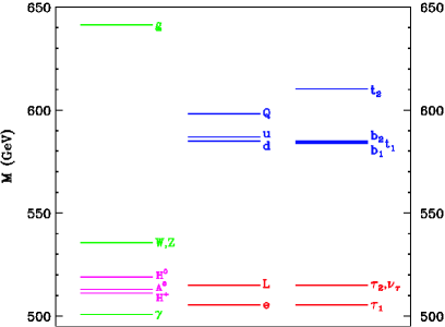
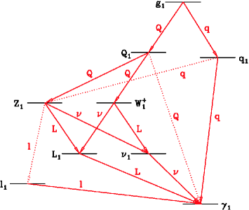
Figure 1: The mass spectrum (left) and the possible decay chains (right) of the first level KK states after taking into account the radiative corrections to the masses [348, 41], for $1/R=500$ GeV. The upper (lower) case fermions represent the doublets (singlets).

3.2 Minimal UED scenario

The minimal UED scenario has only one extra dimension ($\delta=1$). The assumption is made that all boundary terms are negligible at some scale $\Lambda>R^{-1}$. This is completely analogous to the case of the Minimal SUSY SM (MSSM) where one has to choose a set of soft SUSY breaking couplings at some high scale before studying the phenomenology. The choice of boundary couplings may be viewed as analogous to the simplest minimal SUGRA boundary condition: universal scalar and gaugino masses. The minimal UED (MUED) model is extremely predictive, and has only three free parameters:

$$\{R,\Lambda,m_{\mathrm{H}}\}$$

where $m_{\mathrm{H}}$ is the mass of the SM Higgs boson.

The lightest KK particle (LKP) $\gamma_{1}$ (n=1 KK state of the SM photon) is a mixture of the first KK mode $B_{1}$ of the $U(1)_{Y}$ gauge boson $B$ and the first KK mode $W_{1}^{0}$ of the $SU(2)_{W}$ $W^{3}$ gauge boson. The corresponding Weinberg angle $\theta_{1}$ is much smaller than $\theta_{W}$ of the SM, so that the $\gamma_{1}$ is mostly $B_{1}$ and $Z_{1}$ is mostly $W_{1}^{0}$. The spectrum is still quite degenerate, such that the SM particles emitted from these mass splitting decays will be soft. Each level 1 KK particle has an exact analogue in SUSY: $B_{1}\leftrightarrow$ bino, $g_{1}\leftrightarrow$ gluino, $Q_{1}(q_{1})\leftrightarrow$ left-handed (right-handed) squark, etc. The cascade decays of the level 1 KK modes will terminate in the LKP. Just like the neutralino LSP is stable in $R$-parity conserving SUSY, the LKP in MUEDs is stable due to KK parity conservation.

The branching ratios for the different level 1 KK particles are given below, where upper (lower) case fermions represent the doublets (singlets):

$$B(\mathrm{g_{1}\rightarrow Q_{1}Q_{0}})\simeq B(\mathrm{g_{1}\rightarrow q_{1}q_{0}}) \simeq 0.5$$

$$B(\mathrm{q_{1}\rightarrow Z_{1}q_{0}})\simeq\sin^{2}\theta_{1} \simeq 10^{-2}-10^{-3}$$

$$B(\mathrm{q_{1}\rightarrow\gamma_{1}q_{0}})\simeq\cos^{2}\theta_{1} \simeq 1$$

$$B(\mathrm{Q_{1}\rightarrow W_{1}^{\pm}Q_{0}^{\prime}}) \simeq 0.65$$

$$B({Q_{1}\rightarrow Z_{1}Q_{0}}) \simeq 0.33$$

$$B(\mathrm{Q_{1}\rightarrow\gamma_{1}Q_{0}}) \simeq 0.02$$

$$B(\mathrm{W_{1}^{\pm}\rightarrow\nu_{1}L_{0}^{\pm}})=B(\mathrm{W_{1}^{\pm}\rightarrow L_{1}^{\pm}\nu_{0}}) \simeq 1/6\ \mathrm{(for\ each\ generation)}$$

$$B(\mathrm{Z_{1}\rightarrow\nu_{1}\bar{\nu}_{0}})=B(\mathrm{Z_{1}\rightarrow L_{1}^{\pm}L_{0}^{\mp}}) \simeq 1/6\ \mathrm{(for\ each\ generation)}$$

$$B(\mathrm{L_{1}^{\pm}\rightarrow\gamma_{1}L_{0}^{\pm}}) = 1$$

$$B(\mathrm{\nu_{1}\rightarrow\gamma_{1}\nu_{0}}) = 1$$

If they are heavy enough and the phase space is open, the KK Higgs bosons can decay into the KK W and Z bosons or into the KK top and bottom quarks. If they are lighter, their tree-level 2-body decays will be suppressed and they will decay as $\mathrm{H_{1}}\rightarrow\gamma_{1}H_{0}$, or $\mathrm{H_{1}\rightarrow\gamma_{1}\gamma}$ through a loop.

4 GRAVITY MEDIATED DECAYS

We have seen that radiative corrections lift the KK mass degeneracy, and thus induce cascade decays. In addition, some mechanisms can provide for KK decays through gravity mediated interactions [315]. In the latter, the level 1 KK particle decays into its SM equivalent plus a KK graviton. It is interesting to study the phenomenology of a model where both mechanisms occur. If the mass splitting widths of the first level KK excitations are much larger than the gravity mediated widths, the quark and gluon KK excitations cascade down to the LKP ($\gamma_{1}$), which then produces a photon plus a KK graviton. The experimental signal is a striking two photon plus missing energy event.

In the MUED context, the 4+1 dimensional space in which the SM fields propagate may be a thick brane embedded in a space of N $\mathrm{eV}^{-1}$ sized dimensions where only gravitons propagate [315]. The KK excitations can then decay into SM particles plus gravitons going out of the thick brane, and the unbalanced momentum in the extra dimensions can be absorbed by this brane. The lifetime depends on the stength of the coupling to the graviton going out of the brane and the density of its KK modes. Using the decay widths from Macesanu, McMullen and Nandi [349, 350], as well as the KK mass spectrum of the graviton from Beauchemin and Azuelos [351, 352], these type of decays are also considered in the following analysis.

5 Pythia-BASED GENERATOR TOOL

The aim of the work started during the Les Houches 2005 Workshop was to implement the Minimal UED scenario with gravity mediated decays in a generator for future use in the context of the LHC. Some results are shown here for proton-proton collisions at a centre-of-mass energy of 14 TeV. The MUED model, where all SM fields propagate into one ($\delta=1$) TeV^-1 sized extra dimension, embedded in a space of N eV^-1 sized dimensions (where only the graviton propagates), is implemented in the generator tool described below. Hence, mass splitting decays as well as gravity mediated decays are possible.

5.1 Production processes, cross sections and decays

To begin with, the CompHep code [353] with UED implementation [44, 354] was used, where the pair production of KK particles at the LHC is properly described. The generated events (four-vectors of the hard process) were fed into a modified Pythia, where already existing Pythia processes and particles were replaced by those of the KK particle spectrum.

The model was then implemented inside Pythia, as separate new particles as well as new production and decay processes. Table 1 lists the production processes found inside Pythia_UED, where $\mathrm{g}_{1}$ and $\mathrm{Q_{1}}$ ($\mathrm{q_{1}}$) are respectively the first level KK gluon and quark doublet (singlet). The matrix elements of these processes are implemented, as are the masses and widths of the particles, including the one-loop radiative corrections [349, 350].

ISUB	Process	Production source
302	$\mathrm{gg\rightarrow g_{1}g_{1}}$	gg
305	$\mathrm{gg\rightarrow Q_{1}\bar{Q}_{1},q_{1}\bar{q}_{1}}$
303	$\mathrm{gq\rightarrow g_{1}Q_{1},g_{1}q_{1}}$	gq
304	$\mathrm{qq^{\prime}\rightarrow Q_{1}Q_{1}^{\prime},q_{1}q_{1}^{\prime}}$	qq
306	$\mathrm{q\bar{q}\rightarrow Q_{1}\bar{Q}_{1},q_{1}\bar{q}_{1}}$
307	$\mathrm{qq^{\prime}\rightarrow Q_{1}\bar{q}_{1}^{\prime}}$
308	$\mathrm{q\bar{q}^{\prime}\rightarrow Q_{1}\bar{Q}_{1}^{\prime},q_{1}\bar{q}_{1}^{\prime}}$
309	$\mathrm{q\bar{q}^{\prime}\rightarrow Q_{1}Q_{1}^{\prime},q_{1}q_{1}^{\prime}}$
310	$\mathrm{q\bar{q}^{\prime}\rightarrow Q_{1}\bar{Q}_{1}^{\prime},q_{1}\bar{q}_{1}^{\prime}}$

Table 1: Level 1 KK pair production processes, grouped into initial state gg, gq and qq.

The cross-sections versus $M_{KK}=1/R$ are shown in Figure 2 and are in very good agreement with those of Beauchemin and Azuelos [351].

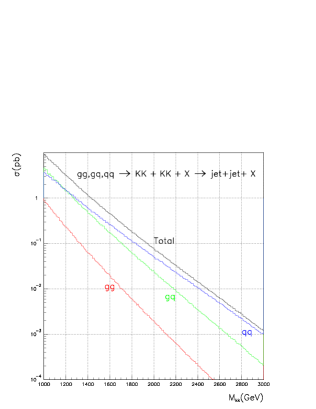
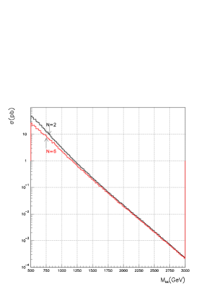
Figure 2: Cross sections for proton-proton collisions and $\mathrm{E_{cm}}=$14 TeV (at the LHC). On the left are shown the cross sections versus $M_{KK}=1/R$ for the production of KK quark pairs. The KK excitations have been forced to decay via gravity mediated decays [$\mathrm{Q_{1}(q_{1})\rightarrow Q(q)+Graviton}$] 100% of the time. The number of $\mathrm{e}V^{-1}$ sized extra dimensions is N=2. Two final state jets are identified with $E_{Tj}>250$ GeV and $E_{j}>$250 GeV. The contributions from the different sources are shown separately: gg, gq and qq. On the right are shown the cross sections for N=2 and 6, where both decay mechanisms are turned on (mass splitting and gravity mediated). Two final state photons are identified with $E_{T\gamma}>200$ GeV.

The mass splitting and gravity mediated decay widths from [348, 41, 355] which are implemented in Pythia_UED are shown in Figure 3.

Figure 3: On the left, the mass splitting decay widths versus $M_{KK}=1/R$ are shown for the level 1 KK excitations of vector bosons : (a)$\mathrm{g_{1}}$, (b) $\mathrm{W_{1}^{\pm}}$ and (c) $\mathrm{Z_{1}}$. The gravity mediated decay widths are shown for (1) N=2 and (2) N=6. On the right, the mass splitting decay widths are shown for the level 1 KK excitations of fermions : (c) $\mathrm{Q_{1}}$, (d) $\mathrm{q_{1}}$ and (e) $\mathrm{L_{1}}$. Again, the gravity mediated decay widths are shown for (1) N=2 and (2) N=6.

5.2 User advice

From the http://wwwlapp.in2p3.fr/$\mathbf{\sim}$przys/PythiaUED.html web page, the pythia_ued_med.tar.gz file can be found, and must be unzipped (i.e. gunzip *.tar.gz) and then untarred (i.e. tar -cvf *.tar). In the main directory, one finds the main routine pkkprod.f, the makefile, and a script comp_exec which compiles or executes pkkprod.f. All other original or modified Pythia routines are in the directory pythia62_ued_rep. In the job_batch directory, a script enables to start KK production jobs.

Various flags can be set in the ued.ini file. This is where the production process can be chosen, as well as the number of eV^-1 sized extra dimensions (N), the values of $1/R$ and $\Lambda$, the flag for turning ON (or OFF) the mass splitting decays, etc. Note that the KK lifetimes are implemented and the vertex information is available.

5.3 Future work

Using the code and model described above, events have been generated and passed through a fast simulation of the ATLAS detector. Preliminary studies have been performed. We are now in the process of producing fully simulated events, in order to study non-pointing photons in the gravity mediated MUED model. These results will be compared with GMSB (Gauge Mediated SUSY Breaking) two photon signals.

6 CONCLUSION AND OUTLOOK

In the context of the LHC, all signals from level 1 KK states can mock SUSY, but identifying the actual nature of the new physics, if it is seen, will be rather challenging. Precision measurements will have to be performed elsewhere than at the LHC. This means that if new physics is seen, the LHC may not be able to disentangle all possible theoretical scenarios which match the data.

Nonetheless, three features could distinguish the MUEDs scenario from ordinary SUSY: the spins will be different, MUEDs do not have analogues of the heavy Higgs bosons of the MSSM, and the signature for MUEDs would be the presence of higher level KK modes.

Acknowledgements

We would like to thank the Les Houches organisation for enabling us to begin this work and for financial support. We thank the following for financial support: Calorimétrie électromagnétique à argon liquide d’ATLAS GDRI between IN2P3/CNRS, the universities Joseph Fourier of Grenoble, of Méditerranée of Aix-Marseille II, and of Savoie, the Moroccan CNRST and KTH Sweden, and the PAI MA/02/38. We thank K. Matchev for useful email exchanges, and K. Matchev and K. Kong for the CompHep-UED code. We thank C.Macesanu for the masses and widths code (radiative corrections and gravity mediated) and for useful email exchanges. And finally, we thank G.Azuelos and P.H.Beauchemin for valuable discussions and inspiration.

Part 18 Les Houches squared event generator for the NMSSM

A. Pukhov and P. Skands

1 INTRODUCTION

With the Tevatron in operation and with the advent of a new generation of colliders on the horison, the LHC and ILC, the exploration of the TeV scale is close at hand. Among the attractive opportunities for a discovery of physics beyond the Standard Model (SM), would be the observation of heavy particles predicted by supersymmetric extensions of the SM (for reviews, see e.g. [356, 357]). The Minimal Supersymmetric Standard Model (MSSM) has been extensively studied, both theoretically and experimentally. Non-minimal SUSY extensions, however, have received less attention. The simplest of them, the Next-to-Minimal Supersymmetric Standard Model (NMSSM, see e.g. [358]), contains one additional supermultiplet, which is a singlet under all the Standard Model gauge groups. From the theoretical point of view the NMSSM solves the naturalness problem, or $\mu$ problem, which plagues the MSSM [359]. From the experimental point of view the NMSSM gives us one additional heavy neutralino and two additional Higgs particles. Moreover, in particular for Higgs physics, the NMSSM can imply quite different ranges of allowed mass values [216] as well as different experimental signatures [219], as compared to the MSSM.

2 NMSSM iN CalcHEP

CalcHEP version 2.4 can be download from
http://theory.sinp.msu.ru/~pukhov/calchep.html
It contains an implementation of the NMSSM [360] and also the NMHDecay code [218, 305]. Apart from the normal range of MSSM parameters (given at the weak scale) the model contains five additional parameters $\lambda$, $\kappa$, $A_{\lambda}$, $A_{\kappa}$, and $\mu_{\mathrm{eff}}=\lambda\left<S\right>$ which describe the Higgs sector, see [218]. For particle codes etc we adopt the conventions of NMHDecay [218]. These conventions are also being adopted for the extension of the SUSY Les Houches Accord [92, 9], reported on elsewhere in these proceedings [361].

CalcHEP [96] is an interactive menu driven program. It allows the user to specify processes, generate and compile the corresponding matrix elements, and to launch the obtained executable. In the given case, CalcHEP launches the nmhdecay_slha code which reads the SLHA input parameter file slhainp.dat, preliminarily prepared by CalcHEP, then calculates the spectrum and writes the SLHA output to a file, spectr.dat. The original SLHA input and output conventions [92] have in this case been suitably extended to include the NMSSM, see [218, 305, 361].

Finally, the program allows to check the spectrum against a large variety of experimental constraints, using NMHDecay. Any constraints that are not satisfied are listed in BLOCK SPINFO in the output spectr.dat file mentioned above. The CalcHEP variable NMHok also displays the number of broken constraints.

3 THE EVENT GENERATION FRAMEWORK

3.1 Hard Scattering

Partonic $2\to N$ events can be generated by CalcHEP using its menu system, and can be stored in a file, by default called events_N.txt. This file contains information about total cross section, Monte Carlo numbers of particles involved, initial energies of beams, partonic distribution functions, and color flows for each event. The first step is thus to generate such a file, containing a number of partonic events for subsequent further processing by a parton shower and hadronisation generator, in our case Pythia [17, 46]. For the interface, we make use of the Les Houches generator accord [362] — see below for details on the implementation.

3.2 Resonance Decays

If the partonic final state passed to Pythia contains heavy unstable particles, a (series of) resonance decay(s) should then follow. However, since Pythia does not internally contain any of the matrix elements relevant to decays involving the new NMSSM states, these partial widths must also first be calculated by some other program, and then be passed to Pythia together with the event file. For this purpose, we use the SUSY Les Houches Accord [92, 9, 361], which includes a possibility to specify decay tables, whereby information on the total width and decay channels of any given particle can be transferred between codes.

Both CalcHEP and NMHDecay can be used to generate such decay tables. For NMHDecay, this file decay.dat is generated automatically, but at present it is limited to the widths and branchings for the Higgs sector only. In the case of CalcHEP the user should start a new session to generate the SLHA file. Here the types of particles are not restricted, but since CalcHEP works exclusively at tree level, Higgs decays to $\mathrm{g}\mathrm{g}$ and $\gamma\gamma$ are absent.

Using the externally calculated partial widths (see below for details on the implementation), we then use the phase space generator inside Pythia, for a particle with appropriate spin, but using an otherwise flat phase space.

3.3 Interface to Pythia

After generating the LHA partonic event file and the SLHA spectrum and decay file, the final step is thus reading this into Pythia and start generating events. The utile\ directory of CalcHEP contains an example main program callPYTH.f which shows how to use CalcHEP’s event2pyth.c routine for reading the event files into Pythia. The most important statements to include are:

C...Specify LHA event file and SLHA spectrum+decay file
      eventFile=’events_1.txt’
      slhafile=’decay.dat’
C...Set up PYTHIA to use SLHA input.
      IMSS(1)=11
C...Open SLHA file
      OPEN(77,FILE=slhafile,STATUS=’OLD’,ERR=100)
C...Tell PYTHIA which unit it is on, both for spectrum and decays
      IMSS(21)=77
      IMSS(22)=77
C...Switch on NMSSM
      IMSS(13)=1
C...Initialize
      NEVMAX=initEvents(eventFile)
      CALL PYINIT(’USER’,’ ’,’ ’,0D0)

To compile everything together, use a linking like the following:

  cc -c event2pyth.c
  f77 -o calcpyth callPYTH.f event2pyth.o pythia6326.f

3.4 Parton Showering, Hadronisation, and Underlying Event

After resonance decays, the event generation proceeds inside Pythia completely as for any other process, i.e. controlled by the normal range of switches and parameters relevant for external processes, see e.g. the recent brief overview in [363]. Specifically, two different shower models are available for comparison, one a virtuality-ordered parton shower and the other a more recently developed transverse-momentum-ordered dipole shower, with each accompanied by its own distinct underlying-event model, see [364, 365] and [366, 367], respectively, and references therein.

At the end of the perturbative stage, at a typical resolution scale of about 1 GeV, the parton shower activity is cut off, and a transition is made to a non–perturbative description of hadronisation, the Pythia one being based on the Lund string model (see [368]). Finally, any unstable hadrons produced in the fragmentation are decayed, at varying levels of sophistication, but again with the possibility of interfacing external packages for specific purposes, such as $\tau$ and $\mathrm{B}$ decays.

4 PRACTICAL DEMONSTRATION

For illustration, we consider Higgs strahlung at the ILC, i.e. the process $\mathrm{e}^{+}\mathrm{e}^{-}\to\mathrm{Z}\mathrm{H}_{1}^{0}$. We concentrate on the difficult scenario discussed in [369], where the lightest Higgs decays mainly to pseudoscalars, and where the pseudoscalars are so light that they cannot decay to $\mathrm{b}$ quarks. As a concrete example of such a scenario, we take “point 1” in [219], with slight modifications so as to give the same phenomenology with NMHDecay version 2.0, with the parameters and masses given in Tab. 1.

pars:	$m_{\mathrm{t}}$	$\mu_{\mathrm{eff}}$	$\lambda$	$\kappa$	$\tan\beta$	$m_{0}$	$M_{1}$	$M_{2}$	$M_{3}$	$A_{\mathrm{b},\mathrm{t},\tau}$	$A_{\lambda}$	$A_{\kappa}$
[GeV]∗	175	-520	0.22	-0.1	5	1000	100	200	700	1500	-700	-2.8

spectrum:	$m_{\mathrm{A}^{0}_{1}}$	$m_{\mathrm{H}^{0}_{1}}$	$m_{\tilde{\chi}^{0}_{1}}$	$m_{\tilde{\chi}^{0}_{2},\tilde{\chi}^{+}_{1}}$	$m_{\tilde{\chi}^{0}_{3}}$	$m_{\mathrm{A}^{0}_{2}}$	$m_{\tilde{\chi}^{0}_{4},\tilde{\chi}^{+}_{2}}$	$m_{\tilde{\chi}^{0}_{5}}$	$m_{\tilde{\mathrm{g}}}$	rest
[GeV]	9.87	89.0	101	200	459	477	530	540	789	$\sim$ 1000

BR’s:	$\mathrm{H}^{0}_{1}\to$	$\mathrm{A}^{0}_{1}\mathrm{A}^{0}_{1}$	$\mathrm{b}\bar{\mathrm{b}}$	$\tau^{+}\tau^{-}$	$\gamma\gamma$	$\mathrm{A}^{0}_{1}\to$	$\tau^{+}\tau^{-}$	$\mathrm{g}\mathrm{g}$	$\mathrm{c}\bar{\mathrm{c}}$	$\mathrm{s}\bar{\mathrm{s}}$
		0.92	0.07	0.006	$8\times 10^{-6}$		0.76	0.21	0.02	0.01

Table 1: Parameters, mass spectrum, and $\mathrm{H}_{1}^{0}/\mathrm{A}_{1}^{0}$ branching ratios larger than 1%, for an NMSSM benchmark point representative of the phenomenology discussed in [369], using NMHDecay 2.0. ${}^{*}:$ in appropriate power of GeV.

We use CalcHEP to compute the basic $\mathrm{e}^{+}\mathrm{e}^{-}\to\mathrm{Z}\mathrm{H}_{1}^{0}$ scattering, NMHDecay to calculate the $\mathrm{H}_{1}^{0}$ and $\mathrm{A}_{1}^{0}$ decay widths, and Pythia for generating the $\mathrm{Z}^{0}$, $\mathrm{H}_{1}^{0}$, and $\mathrm{A}_{1}^{0}$ decays as well as for subsequent $\tau$ decays, bremsstrahlung, and hadronisation.

We generate 30000 events at the $\mathrm{e}^{+}\mathrm{e}^{-}\to\mathrm{Z}^{0}\mathrm{H}^{0}_{1}$ level, at $\sqrt{s}=500$ GeV corresponding to about $500\leavevmode\nobreak\ \mathrm{fb}^{-1}$ of integrated luminosity. Out of these, we select events with 4 tauons in the final state (with $p_{\perp}>5$ GeV) and where the $\mathrm{Z}$ does not decay to neutrinos. The plot in Fig. 1 shows simultaneously the invariant mass distributions of $\tau^{+}\tau^{-}$ (solid, green) $\tau^{+}\tau^{-}\tau^{+}\tau^{-}$ (dot-dashed, red), and $\mathrm{b}\bar{\mathrm{b}}$ (dashed, blue) for these events.

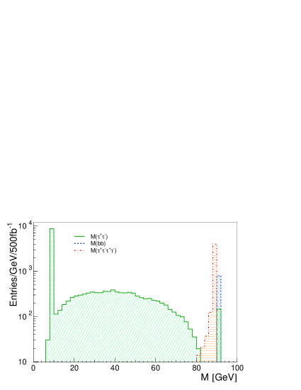
Figure 1: Invariant masses for 2-$\tau$ (solid, green), $\mathrm{b}\bar{\mathrm{b}}$ (dashed, blue), and 4-$\tau$ (dot-dashed, red) combinations in $\mathrm{e}^{+}\mathrm{e}^{-}\to\mathrm{H}_{1}^{0}\mathrm{Z}^{0}$ events at $\sqrt{s}=500$ GeV, requiring 4 tauons with $p_{\perp}>5$ GeV in the final state and $\mathrm{Z}^{0}\to$ visible.

Of course, experiments do not observe tauons and $\mathrm{b}$ quarks directly; this plot is merely meant to illustrate that the expected resonance peaks appear where they should: firstly, a large $\tau^{+}\tau^{-}$ peak at the $\mathrm{A}^{0}$ mass, and a smaller one at the $\mathrm{Z}^{0}$ mass. Secondly, a $\mathrm{b}\bar{\mathrm{b}}$ peak also at the $\mathrm{Z}^{0}$ mass and finally the 4-$\tau$ peak at the $\mathrm{H}^{0}_{1}$ mass.

5 CONCLUSION

We present a framework intended for detailed studies of the collider phenomenology of NMSSM models. We combine three codes developed independently to obtain a full-fledged event generator for the NMSSM, including hard scattering, resonance decays, parton showering, and hadronisation. The interface itself is fairly straightforward, relying on standards developed at previous Les Houches workshops.

Moreover, it seems clear that this application should only be perceived as a first step. With slight further developments, a more generic framework seems realisable, which could greatly facilitate the creation of tools for a much broader range of beyond the Standard Model physics scenarios. In particular we would propose to extend the SLHA spectrum and decay file structures to include all the information that defines a particle — specifically its spin, colour and electric quantum numbers, in addition to its mass and decay modes. This would make it possible for a showering generator to handle not just the particles it already knows about, but also more generic new states.

Acknowledgements

We are grateful to U. Ellwanger for many helpful suggestions, including the NMSSM parameters used for the benchmark point. Many thanks also to the organizers of the Physics at TeV Colliders workshop, Les Houches, 2005. This work was supported by Universities Research Association Inc. under Contract No. DE-AC02-76CH03000 with the United States Department of Energy.

Part 19 The MSSM implementation in SHERPA

S. Schumann

1 INTRODUCTION

SHERPA [316] is a multi-purpose Monte Carlo event generator that is able to simulate high-energetic collisions at lepton and hadron colliders. The code is publicly available and can be downloaded from http://www.sherpa-mc.de.

The physics programme of SHERPA covers:

• The description of hard processes in the framework of the Standard Model, the Minimal Supersymmetric Standard Model and the ADD model of large extra dimensions using tree level matrix elements provided by the matrix element generator AMEGIC++ [370, 371, 318].

• Multiple QCD bremsstrahlung from initial and final state partons taken care of by the parton shower program APACIC++ [372].

• The merging of matrix elements and parton showers according to the CKKW prescription [373].

• Jet fragmentation and hadronisation provided by an interface to corresponding PYTHIA routines.

• The inclusion of hard underlying events similar to the description in [364].

In the following the spot will solely be on aspects related to the implementation of the MSSM in SHERPA.

2 THE MSSM IMPLEMENTATION

The central part of the MSSM implementation in SHERPA is the extension of the internal matrix element generator AMEGIC++ to cover the Feynman rules of the physics model. For this task the very general set of Ref. [374] for the $R$-parity conserving MSSM has been implemented. These Feynman rules allow for a general form of flavour mixing in the SUSY sector and permit the inclusion of CP violating parameters. Beyond this they include finite masses and Yukawa couplings for all the three fermion generations. From these Feynman rules AMEGIC++ automatically constructs all the Feynman diagrams contributing to a given process in the tree-level approximation. The generated Feynman diagrams then get translated into helicity amplitudes that are written into library files. In conjunction appropriate phase space mappings are generated, and stored as library files as well, which are used during integration and the procedure of event generation. Note that no narrow-width approximation or the like is assumed, the amplitudes contain all the resonant as well as non-resonant contributions that may contribute. Due to the usage of exact Feynman diagrams the algorithm includes spin-correlations in the most natural way. To unambiguously fix the relative signs amongst Feynman diagrams involving Majorana spinors the algorithm described in [375] has been implemented. For the negative mass eigenvalues appearing in the diagonalisation of the neutralino mixing matrix the helicity formalism allows to directly take them into account in the propagators and spinor products used. This way a redefinition of the neutralino fields and couplings can be avoided.

To calculate the couplings of the Feynman rules the program needs to be supplemented with a full set of weak-scale parameters. Since version SHERPA-1.0.7 this can be done using a SUSY Les Houches Accord [92] conform file whose parameters are translated to the conventions of [374] by the program.

3 CONCLUSIONS

The SHERPA generator with the MSSM implemented as described above provides a powerful tool for the description of supersymmetric processes at lepton and hadron colliders, see for instance [376, 289, 317]. It allows for the realistic description of multi-particle final states related to sparticle production processes by fully taking into account off-shell effects as well as non-resonant contributions and thereby preserving all spin correlations present.

At present the incorporation of interactions originating from bilinearly broken $R$-parity is ongoing. The helicity formalism used within AMEGIC++ is currently extended to cover spin-$3/2$ particles as well. Upon completion this will then allow for the simulation of supersymmetric processes involving gravitinos.

Part 20 High precision calculations in the MSSM Higgs sector with FeynHiggs2.3

T. Hahn, S. Heinemeyer, W. Hollik, H. Rzehak and G. Weiglein

1 INTRODUCTION

The search for the lightest Higgs boson is a crucial test of Supersymmetry (SUSY) which can be performed with the present and the next generation of accelerators. Especially for the Minimal Supersymmetric Standard Model (MSSM) a precise prediction for the masses of the Higgs bosons and their decay widths in terms of the relevant SUSY parameters is necessary in order to determine the discovery and exclusion potential of the Tevatron, and for physics at the LHC and the ILC. In the case of the MSSM with complex parameters (cMSSM) the task is even more involved. Several parameters can have non-vanishing phases. These are the Higgs mixing parameter $\mu$, the trilinear couplings $A_{f}$, $f=t,b,\tau,\ldots$, and the gaugino masses $M_{1}$, $M_{2}$, $M_{3}\equiv m_{\tilde{g}}$ (the gluino mass parameter). Furthermore the neutral Higgs bosons are no longer ${\cal CP}$-eigenstates, but mix with each other once loop corrections are taken into account [291].

$$(h,H,A)\to(h_{1},h_{2},h_{3})\leavevmode\nobreak\ \leavevmode\nobreak\ \leavevmode\nobreak\ {\rm with}\leavevmode\nobreak\ \leavevmode\nobreak\ \leavevmode\nobreak\ m_{h_{1}}\leq m_{h_{2}}\leq m_{h_{3}}\,.$$ (1)

The input parameters within the Higgs sector are then (besides the Standard Model (SM) ones) $\tan\beta$, the ratio of the two vacuum expectation values, and the mass of the charged Higgs boson, $M_{H^{\pm}}$.

2 THE CODE FeynHiggs

FeynHiggs [300, 155, 156] is a Fortran code for the computation of masses and mixing angles in the MSSM with real or complex parameters. The calculation of the higher-order corrections is based on the Feynman-diagrammatic approach [277]. At the one-loop level, it consists a complete evaluation of the self-energies (with a hybrid $\overline{\rm{MS}}$ /on-shell scheme renormalization). At the two-loop level all existing corrections from the real MSSM have been included (see Ref. [156] for a review), supplemented by the resummation of the leading effects from the (scalar) $b$ sector including the full phase dependence. As a new feature the Higgs masses are determined from the complex propagator matrix.

Besides the evaluation of the Higgs-boson masses and mixing angles, the program also includes the estimation of the theory uncertainties of the Higgs masses and mixings due to missing higher-order corrections. The total uncertainty is the sum of deviations from the central value, $\Delta X=\sum_{i=1}^{3}|X_{i}-X|$ with $X=\{M_{h_{1},h_{2},h_{3},H^{\pm}},U_{ij}\}$, where the $X_{i}$ are obtained by:

• $X_{1}$: varying the renormalization scale (entering via the $\overline{\rm DR}$ ren.) within $1/2m_{t}\leq\mu\leq 2m_{t}$,

• $X_{2}$: using $m_{t}^{\rm pole}$ instead of the running $m_{t}$ in the two-loop corrections,

• $X_{3}$: using an unresummed bottom Yukawa coupling, $y_{b}$, i.e. an $y_{b}$ including the leading ${\cal O}(\alpha_{s}\alpha_{b})$ corrections, but not resummed to all orders.

Furthermore FeynHiggs2.3 contains the computation of all relevant Higgs-boson decay widths and hadron collider production cross sections. These are in particular:

• the total width for the three neutral and the charged Higgs bosons,

• the couplings and branching ratios of the neutral Higgs bosons to

  • SM fermions $h_{i}\to\bar{f}f$,

  • SM gauge bosons (possibly off-shell), $h_{i}\to\gamma\gamma,ZZ^{*},WW^{*},gg$,

  • gauge and Higgs bosons, $h_{i}\to Zh_{j}$, $h_{i}\to h_{j}h_{k}$,

  • scalar fermions, $h_{i}\to\tilde{f}^{\dagger}\tilde{f}$,

  • gauginos, $h_{i}\to\tilde{\chi}^{\pm}_{k}\tilde{\chi}^{\mp}_{j}$, $h_{i}\to\tilde{\chi}^{0}_{l}\tilde{\chi}^{0}_{m}$,

• the couplings and branching ratios of the charged Higgs boson to

  • SM fermions, $H^{-}\to\bar{f}f^{\prime}$,

  • a gauge and Higgs boson, $H^{-}\to h_{i}W^{-}$,

  • scalar fermions, $H^{-}\to\tilde{f}^{\dagger}\tilde{f}^{\prime}$,

  • gauginos, $H^{-}\to\tilde{\chi}^{-}_{k}\tilde{\chi}^{0}_{l}$,

• the neutral Higgs-boson production cross-sections at the Tevatron and the LHC for all relevant channels.

For comparisons with the SM, the following quantities are also evaluated for SM Higgs bosons with the same mass as the three neutral MSSM Higgs bosons:

• the total decay widths,

• the couplings and BRs of a SM Higgs boson to SM fermions,

• the couplings and BRs of a SM Higgs boson to SM gauge bosons (possibly off-shell),

• the production cross-sections at the Tevatron and the LHC for all relevant channels.

For constraining the SUSY parameter space, the following electroweak precision observables are computed (see Ref. [257] and references therein),

• the $\rho$-parameter up to the two-loop level that indicates disfavored scalar top and bottom masses

• the anomalous magnetic moment of the muon.

Finally, FeynHiggs2.3 possesses some further features:

• Transformation of the input parameters from the $\overline{\rm{DR}}$ to the on-shell scheme (for the scalar top and bottom parameters), including the full ${\cal O}(\alpha_{s})$ and ${\cal O}(\alpha_{t,b})$ corrections.

• Processing of SUSY Les Houches Accord (SLHA) data [92, 332]. FeynHiggs2.3 reads the output of a spectrum generator file and evaluates the Higgs boson masses, brachning ratios etc. The results are written in the SLHA format to a new output file.

• Predefined input files for the SPS benchmark scenarios [45] and the Les Houches benchmarks for Higgs-boson searches at hadron colliders [377] are included.

• Detailed information about the features of FeynHiggs2.3 are provided in man pages and a manual.

3 INSTALLATION AND USE

The installation process is straightforward and should take no more than a few minutes:

• Download the latest version from www.feynhiggs.de and unpack the tar archive.

• The package is built with ./configure and make. This creates the library libFH.a and the command-line frontend FeynHiggs.

• To build also the Mathematica frontend MFeynHiggs, invoke make all.

• make install installs the files into a platform-dependent directory tree, for example
  i586-linux/{bin,lib,include}.

• Finally, remove the intermediate files with make clean.

FeynHiggs2.3 has four modes of operation,

• Library Mode: Invoke the FeynHiggs routines from a Fortran or C/C++ program linked against the libFH.a library.

• Command-line Mode: Process parameter files in native FeynHiggs or SLHA format at the shell prompt or in scripts with the standalone executable FeynHiggs.

• WWW Mode: Interactively choose the parameters at the FeynHiggs User Control Center (FHUCC) and obtain the results on-line.

• Mathematica Mode: Access the FeynHiggs routines in Mathematica via MathLink
  (MFeynHiggs).

3.1 Library Mode

The core functionality of FeynHiggs2.3 is implemented in a static Fortran 77 library libFH.a. All other interfaces are ‘just’ frontends to this library.

In view of Fortran’s lack of symbol scoping, all internal symbols have been prefixed to make symbol collisions very unlikely. Also, the library contains only subroutines, no functions, which simplifies the invocation. In Fortran, no include files are needed except for access to the coupling structure (FHCouplings.h). In C/C++, a single file CFeynHiggs.h must be included once for the prototypes. Detailed debugging output can be turned on at run time.

The library provides the following functions:

• FHSetFlags sets the flags for the calculation.

• FHSetPara sets the input parameters directly, or
  FHSetSLHA sets the input parameters from SLHA data.

• FHSetDebug sets the debugging level.

• FHGetPara retrieves (some of) the MSSM parameters calculated from the input parameters, e.g.  the sfermion masses.

• FHHiggsCorr computes the corrected Higgs masses and mixings.

• FHUncertainties estimates the uncertainties of the Higgs masses and mixings.

• FHCouplings computes the Higgs couplings and BRs.

• FHConstraints evaluates further electroweak precision observables.

These functions are described in detail on their respective man pages in the FeynHiggs package.

3.2 Command-line Mode

The FeynHiggs executable is a command-line frontend to the libFH.a library. It is invoked at the shell prompt as
   FeynHiggs inputfile [flags] [scalefactor]
where

• inputfile is the name of a parameter file (see below).

• flags is an (optional) string of integers giving the flag values, e.g.  40030211.

• scalefactor is an optional factor multiplying the renormalization scale.

FeynHiggs understands two kinds of parameter files:

• Files in SUSY Les Houches Accord (SLHA) format. In this case FeynHiggs adds the Higgs masses and mixings to the SLHA data structure and writes the latter to a file inputfile.fh.

  In fact, FeynHiggs tries to read each file in SLHA format first, and if that fails, falls back to its native format.

• Files in its native format, for example

    MT         174.3
    MB         4.7
  

    MSusy      500
    MA0        200
    Abs(M_2)   200
    Abs(MUE)   1000
    TB         5
    Abs(Xt)    1000
    Abs(M_3)   800
  

  Complex quantities can be given either in terms of absolute value Abs(X) and phase Arg(X), or as real part Re(X) and imaginary part Im(X). Abbreviations, summarizing several parameters (such as MSusy) can be used, or detailed information about the various soft SUSY-breaking parameters can be given. Furthermore, it is possible to define loops over parameters, to scan parts of parameter space.

  The output is written in a human-readable form to the screen. It can also be piped through the table filter to yield a machine-readable version appropriate for plotting etc. For example,

    FeynHiggs inputfile flags | table TB Mh0 > outputfile
  

  creates outputfile with two columns, $\tan\beta$ and $m_{h^{0}}$. The syntax of the output file is given as screen output.

3.3 WWW Mode

The FeynHiggs User Control Center (FHUCC) is a WWW interface to the command-line executable FeynHiggs. To use the FHUCC, point your favorite Web browser at

www.feynhiggs.de/fhucc.

3.4 Mathematica Mode

The MFeynHiggs executable provides access to the FeynHiggs functions from Mathematica via the MathLink protocol. After starting Mathematica, install the package with
   In[1]:= Install["MFeynHiggs"]
which makes all FeynHiggs subroutines available as Mathematica functions.

Part 21 micrOMEGAs2.0 and the relic density of dark matter in a generic model

G. Bélanger, F. Boudjema, A. Pukhov and A. Semenov

1 INTRODUCTION

Precision cosmological measurements have recently provided very powerful tests on the physics beyond the standard model. In particular the WMAP measurement of the relic density of dark matter [2, 3] now provides some of the most stringent constraints on supersymmetric models with R-parity conservation. The large number of existing studies on the impact of a measurement of the relic density on models of new physics have concentrated on the minimal supersymmetric standard model[85] and especially on mSUGRA, an underlying model defined at the high scale [4, 8, 84, 86, 87]. Furthermore, all the publicly available codes, including the 3 state-of-the art codes micrOMEGAs[5, 6], DarkSUSY[326] and IsaTools[378] that compute the relic density of dark matter, also only work within the context of the general MSSM or high scale models such as mSUGRA. On the other hand, one can show, based on general arguments [379], that reasonable values for the relic density can be obtained in any model with a stable particle which is weakly interacting. Candidates for dark matter then go far beyond the much studied neutralino-LSP in supersymmetric models. Explicit examples include a model with universal extra dimensions [380, 381], models with warped extra dimensions[382], or little Higgs models [383]. Furthermore, studies of relic density of dark matter in some generalizations of the MSSM such as the MSSM with CP violation[91, 89] or the NMSSM which contains an extra singlet [360, 384] or even the MSSM with an extra U(1)[385], all emphasize the presence of new channels that can lead to a reasonable value of the relic density of dark matter where it was not possible within the MSSM. In all these models, a discrete symmetry like R-parity conservation ensures the stability of the lightest odd particle(LOP) .

Considering the wealth of models with suitable dark matter candidates, it becomes interesting to provide a tool to calculate the relic density of dark matter in an arbitrary model. Since micrOMEGAs is based on CalcHEP [96] a program that automatically calculates cross sections in a given model, it becomes in principle straightforward to make the corresponding adaptation of the micrOMEGAs  code. Here we briefly review the relic density calculation before discussing the implementation of new models in micrOMEGAs2.0, including the MSSM and NMSSM as examples.

2 CALCULATION OF RELIC DENSITY

A relic density calculation entails solving the evolution equation for the abundance of the dark matter, $Y(T)$, defined as the number density divided by the entropy density, (here we follow closely the approach in [386, 387])

$$\frac{dY}{dT}=\sqrt{\frac{\pi g_{*}(T)}{45}}M_{p}<\sigma v>(Y(T)^{2}-Y_{eq}(T)^{2})$$ (1)

where $g_{*}$ is an effective number of degree of freedom [386], $M_{p}$ is the Planck mass and $Y_{eq}(T)$ the thermal equilibrium abundance. $<\sigma v>$ is the relativistic thermally averaged annihilation cross-section. The dependence on the specific model for particle physics enters only in this cross-section which includes all channels for annihilation and coannihilation,

$$<\sigma v>=\frac{\sum\limits_{i,j}g_{i}g_{j}\int\limits_{(m_{i}+m_{j})^{2}}ds\sqrt{s}K_{1}(\sqrt{s}/T)p_{ij}^{2}\sigma_{ij}(s)}{2T\big{(}\sum\limits_{i}g_{i}m_{i}^{2}K_{2}(m_{i}/T)\big{)}^{2}}\;,$$ (2)

where $g_{i}$ is the number of degree of freedom, $\sigma_{ij}$ the total cross section for annihilation of a pair of R-parity odd particles with masses $m_{i}$, $m_{j}$ into some R-parity even particles, and $p_{ij}(\sqrt{s})$ is the momentum (total energy) of the incoming particles in their center-of-mass frame.

Integrating Eq. 1 from $T=\infty$ to $T=T_{0}$ leads to the present day abundance $Y(T_{0})$ needed in the estimation of the relic density,

$$\Omega_{LSP}h^{2}=\frac{8\pi}{3}\frac{s(T_{0})}{M_{p}^{2}(100{\rm(km/s/Mpc)})^{2}}M_{LSP}Y(T_{0})=2.742\times 10^{8}\frac{M_{LSP}}{GeV}Y(T_{0})$$ (3)

where $s(T_{0})$ is the entropy density at present time and $h$ the normalized Hubble constant.

In the framework of the MSSM, the computation of all annihilation and coannihilation cross-sections are done exactly at tree-level. For this we rely on CalcHEP [96], a generic program which once given a model file containing the list of particles, their masses and the associated Feynman rules describing their interactions, computes any cross-section in the model. To generalize this program to other particle physics models one only needs to replace the calculation of the thermally averaged annihilation cross-section for the stable particle that plays the role of dark matter. This can be done easily after specifying the new model file into CalcHEP. Then to solve numerically the evolution equation and calculate $\Omega h^{2}$ one uses the standard micrOMEGAs  routines.

In order that the program finds the list of processes that need to be computed for the effective annihilation cross-section, one needs to specify the analogous of R-parity and assign a parity odd or even to all particles. The lightest odd particle will then be identified to the dark matter candidate. All possible processes will be identified and computed automatically, imposing R-parity conservation. The program will then look automatically for poles, such as Higgses or Z’, and thresholds and adapt the integration routines for higher accuracies in these specific regions.

Another advantage of our approach based on a generic program like CalcHEP is that one can compute in addition any cross-sections or decay widths in the new model considered. In particular, tree-level cross-sections for $2\rightarrow 2$ processes and 2-body decay widths of particles are available. Furthermore the cross-sections times relative velocity, $\sigma v$, for neutralino annihilation at $v\rightarrow 0$ and the yields for $\gamma,e^{+},\bar{p}$, relevant for indirect detection of neutralinos, are also automatically computed.

3 micrOMEGAs2.0

3.1 MSSM

A public version for relic density calculations in the MSSM has been available for a few years and has been upgraded to micrOMEGAs1.3 [6], which most importantly incorporates some higher-order effects. For one we use loop corrected superparticle masses and mixing matrices. These masses and mixing matrices, as specified in the SUSY Les Houches Accord (SLHA)[92], are then used to compute exactly all annihilation/coannihilation cross-sections. This can be done whether the input parameters are specified at the weak scale or at the GUT scale in the context of SUGRA models or the like. In the last case, loop corrections are obtained from one of the public codes which calculate the supersymmetric spectrum using renormalization group equations (RGE) [62, 319, 35, 7]. Higher order corrections to the Higgs masses are also calculated by one of the spectrum calculators. QCD corrections to Higgs partial widths are included as well as the important SUSY corrections, the $\Delta m_{b}$ correction, that are relevant at large $\tan\beta$. These higher-order corrections also affect directly the Higgs-$q\overline{q}$ vertices and are taken into account in all the relevant annihilation cross-sections. External routines that provide constraints on supersymmetric models such as $(g-2)_{\mu}$, $\delta\rho$, $b\rightarrow s\gamma$ and $B_{s}\rightarrow\mu^{+}\mu^{-}$ are also included.

3.2 NMSSM

The NMSSM is the simplest extension of the MSSM with one extra singlet. A new model file was implemented into CalcHEP and as in the MSSM, an improved effective potential for the Higgs sector was defined. The parameters of this potential are derived from the physical masses and mixing matrices that are provided by an external program, here NMHDECAY [218]. Some experimental and theoretical constraints on the model are also checked by NMHDECAY. The input parameters of the model and more details on the model are described in Ref. [360]. The new functions specific to the NMSSM are given in the Appendix.

3.3 Other models

In general, to implement a new model the user only needs to include the CalcHEP model files in the sub directory work/models. More precisely the model must include four files that specify the list of particles(prtcls1.mdl), the independent variables(vars1.mdl), the Lagrangian with all vertices(lgrng1.mdl) and all internal functions(func1.mdl). Note that to automatize as much as possible the procedure for creating a new model, it is possible to use a program like LanHEP[95], which starts from a Lagrangian in a human readable format and derives all the necessary Feynman rules . Alternatively the user can write by hand the model files of the new model. A complete CalcHEP model might also require additional internal functions, these should be included in the directory lib. Examples of such specific functions already provided in the MSSM include, routines to calculate the supersymmetric spectrum starting from a reduced set of parameters defined at the GUT scale or routines to calculate constraints, such as $b\rightarrow s\gamma$. Slight modifications to the standard CalcHEP model files are necessary. A * before the masses and widths of R-parity odd particles must be inserted in the relevant file as well as a ! before the widths of particles that can appear in s-channel in any of the (co)-annihilation processes. The latter is to enabled automatic width calculation.

All other files and subdirectories are generated automatically and do not need to be modified by the user. They contain, in addition to temporary files, the libraries of matrix elements generated by CalcHEP. By default the list of R-parity odd particles will be constructed and will include all particles whose name starts by ~. This list is stored in odd_particles.c and can be modified by the user. While executing the Makefile, a call to CalcHEP will generate all processes of the type

$$\sim\chi_{i}\sim\chi_{j}\rightarrow X,Y$$

where $\sim\chi_{i}$ designates all R-parity odd particle and X,Y all R-parity even particles. In practice only processes involving the LOP as well as those particles for which $m_{\chi_{i}}<1.5m_{LOP}$. As in previous versions of micrOMEGAs , new processes are compiled and added only when necessary, in run-time.

3.4 Installation

micrOMEGAs  can be obtained at
                 http://wwwlapp.in2p3.fr/lapth/micromegas

together with some instructions on how to install and execute the program. The name of the file downloaded should be micromegas_2.0.tgz. After unpacking the code one only needs to launch the micro_make command. For using the MSSM or NMSSM version the user must first go to the appropriate directory. The executable is generated by the command make main=main.c for any of the main programs provided.

To create a new model, one has to launch the command micromake NewModel which will create the directory NewModel containing two directories, /work and /lib as well as two sample main programs to calculate the relic density, omg.c,omg.F. A Makefile is also generated by this call.

4 CONCLUSION

micrOMEGAs2.0 is a new and versatile tool to calculate the relic density of dark matter in a generic model of particle physics that contains some analog of R-parity to ensure the stability of the lightest particle. The existing versions of micrOMEGAs  for the MSSM and the NMSSM have been implemented in this framework. We have briefly described here how this could be extended to other models. Examples of other models that are being implemented in micrOMEGAs  are the MSSM model with CP violation, the model with Universal Extra dimensions as well as the warped extra dimension model with stable Kaluza-Klein particle.

Acknowledgements

This work was supported in part by GDRI-ACPP of CNRS and by grants from the Russian Federal Agency for Science, NS-1685.2003.2 and RFBR-04-02-17448. We thank C. Balazs, S. Kraml, C. Hugonie, G. Servant, W. Porod for useful discussions and for testing parts of this program.

blabla

NON-SUSY BSM

Part 22 NON SUSY BSM

C. Grojean

The legacy of LEP/SLC is an impressive triumph of human endeavor with the validation of the quantum nature of the Standard Model (SM) to its highest accuracy. Still, and despite all expectations, it leaves us with the most pressing question: How do elementary particles acquire a mass? How is electroweak symmetry broken? The usual SM Higgs mechanism jeopardizes our current understanding of the SM at the quantum level and electroweak precision measurements seriously contrive any extension beyond it. Better than a long introduction, the following tautology reveals that an understanding of the dynamics of electroweak symmetry breaking (EWSB) is still missing

Why is EW symmetry broken?

because the Higgs potential is unstable at the origin

Why is the Higgs potential unstable at the origin?

because otherwise EW symmetry wouldn’t be broken

One should understand that the SM Higgs mechanism is only a description of EWSB and not an explanation of it since in particular there is no dynamics to explain the instability at the origin. The hierarchy problem tells us that it is less and less natural that no new particles emerge as we explore higher and higher energy. At the same time, however, electroweak precision measurements severely constrain the existence of such new particles. These constraints are nowadays so severe that the minimal supersymmetric standard model considered for a long time as the paradigm of BSM physics does not appear more natural than 1 in 100, in the absence of any anthropic selection. At the eve of LHC, this pang of conscience could have been quite discouraging. On the contrary it has stimulated the creativity of the BSM physicists and in the last few years numerous new ideas have emerged both on the phenomenological and the theoretical sides.

Non-susy BSM benchmark models popped up: by now ADD and RS models have become unavoidable for any student starting his/her PhD. The real achievement of these models was to bring new tools to address old problems. Any paradigm cannot be a solution and benchmark scenarios daily evolve to incorporate new features that make them more and more realistic: the original ADD and RS models have been considerably amended in their up to-date incarnations.

These proceedings are an introductory collection to new models that emerged in the past few years as well as a tentative identification of experimental signatures.

Part 23 presents models with TeV size extra dimensions accessible to all SM particles. Part 24 elaborates on models with TeV size extra dimensions in which the SM fermions are localized close to the boundaries of the extra dimensions. Part 25 addresses the issue of Dark Matter in models with extra dimensions and relates the existence of a DM candidate to a symmetry that ensures the proton stability.

Part 26 introduces models where the Higgs appears as a component of the gauge field along an extra dimension. Higher dimensional gauge invariance then forbids any local mass counter term in the Higgs potential which is thus finite and calculable.

Part 27 presents Little Higgs models that make the Higgs a pseudo-Goldstone boson. The radiative corrections in the Higgs potential are now severely constrained by a Peccei–Quinn shift symmetry. Part 28 carries on a Monte Carlo study of the Littlest Higgs model and evaluates the discovery potential at LHC. Any Little Higgs model predicts the existence of a top partner to cancel the divergent contribution to the Higgs mass from the top loop. Part 29 proposes to look at the polarization of the third generation family to pin down the properties of the top partner.

Part 30 is a general analysis of a Higgs sector that would contain charged scalars, as it is the case in Little Higgs models and other models. A careful selection of variables has to be used to separate the signal from the background.

Part 31 looks for the diphoton production in the RS model as a result of the KK graviton interactions.

Part 32 presents Higgsless models where EWSB is triggered by boundary condition rather than by a usual Higgs mechanism. It is shown that the tower of massive KK gauge bosons unitarizes the scattering amplitude of longitudinal polarized gauge bosons. Finally Part 33 examines, with a full detector simulation, the reconstruction of $WZ$ resonances in a Higgsless model as well as in a chiral lagrangian model.

The workshop was an ideal opportunity to gather model builders and experimentalists. Back home, these proceedings should help us to work closer together.

Part 23 Universal extra dimensions at hadron colliders

B.A. Dobrescu

The Standard Model is a quantum field theory that has an $SU(3)\times SU(2)\times U(1)$ gauge symmetry and an $SO(1,3)$ Lorentz symmetry. The possibility that the Lagrangian describing nature has a larger gauge symmetry has very often been studied. However, it is also very interesting to study the possibility that the Lagrangian has an extended Lorentz symmetry. The most obvious extended Lorentz symmetry is $SO(1,3+n)$ with $n\geq 1$ an integer. This implies that all Standard Model particles propagate in $n$ extra spatial dimensions endowed with a flat metric. These are called universal extra dimensions [314], and lead to a phenomenology completely different than extra dimensions accessible only to gravity or only to bosons (see the chapter on “Models with localized fermions”).

Given that no extra dimensions have been observed yet, they must be compactified with a size smaller than the resolution of current experiments. Compactification implies that the extended Lorentz symmetry is broken by the boundary conditions down to the $SO(1,3)$ Lorentz symmetry, although an additional subgroup may also be preserved.

Any quantum field propagating in a space with boundaries is a superposition of a discrete set of states of definite momentum. Therefore, the $(4+n)$-dimensional fields may be expanded in terms of 4-dimensional fields, called Kaluza-Klein (KK) modes, with definite momentum along the extra dimensions. The search in collider experiments of KK modes having a spectrum and interactions consistent with a certain compactification is the best way of checking the existence of extra dimensions.

An important feature of the Standard Model is that its fermions are chiral, which means that the left- and right-handed components of any Dirac fermion have different gauge quantum numbers. This imposes a constraint on the compactification of universal extra dimensions, because the simplest compactifications, on a circle or a torus, always lead to non-chiral (“vectorlike”) fermions. The chirality of the four-dimensional fermions has to be introduced by the boundary conditions.

Gauge theories in more than four spacetime dimensions are nonrenormalizable. This is not a problem as long as there is a range of scales where the higher-dimensional field theory is valid. For gauge couplings of order unity, as in the Standard model, the range of scales is of the order of $(4\pi)^{2/n}$, so that only low values of $n$ are interesting. Furthermore, the low energy observables get corrections from loops with KK modes. The leading corrections are finite in the $n=1$ case and logarithmically divergent for $n=2$, while for $n\geq 3$ they depend quadratically or stronger on the cut-off. Therefore, the effects of the unknown physics above the cut-off scale can be kept under control only for $n=1$ and $n=2$.

The majority of phenomenological studies related to universal extra dimensions have concentrated on the $n=1$ case. The extra dimension is an interval (see Figure 1), and the boundary conditions at its end points determine the spectrum of KK modes.

Figure 1: The extra dimension of coordinate $y$ extends from $y=0$ to $y=\pi R$.

The Kaluza-Klein modes of a Standard Model particle of mass $m_{0}$ form a tower of four-dimensional particles of masses

$$M_{j}=\sqrt{m_{0}^{2}+\frac{j^{2}}{R^{2}}}\leavevmode\nobreak\ ,$$ (1)

where $j\geq 0$ is an integer called the KK number. The $j=0$ states are called zero-modes; their wave functions are flat along the extra dimension. The zero-modes are identified with the usual Standard Model particles.

A five-dimensional gauge boson has five components: $A_{\mu}(x^{\nu},y)$, $\mu,\nu=0,1,2,3$, and $A_{y}(x^{\nu},y)$ which corresponds to the polarization along the extra dimension. The coordinates $x^{\nu}$ refer to the usual four spacetime dimensions, and $y$ is the coordinate along the extra dimension, which is transverse to the non-compact ones. From the point of view of the four-dimensional theory, $A_{y}(x^{\nu},y)$ is a tower of spinless KK modes. The boundary conditions are given by

$$\frac{\partial}{\partial y}A_{\mu}(x^{\nu},0)=\frac{\partial}{\partial y}A_{\mu}(x^{\nu},\pi R)=0\leavevmode\nobreak\ ,$$

$$A_{y}(x,0)=A_{y}(x,\pi R)=0\leavevmode\nobreak\ .$$ (2)

Solving the field equations with these boundary conditions yields the following KK expansions:

$$A_{\mu}(x^{\nu},y)=\frac{1}{\sqrt{\pi R}}\left[A_{\mu}^{(0)}(x^{\nu})+\sqrt{2}\sum_{j\geq 1}A_{\mu}^{(j)}(x^{\nu})\cos\left(\frac{jy}{R}\right)\right]\leavevmode\nobreak\ ,$$

$$A_{y}(x^{\nu},y)=\sqrt{\frac{2}{\pi R}}\sum_{j\geq 1}A_{y}^{(j)}(x^{\nu})\sin\left(\frac{jy}{R}\right)\leavevmode\nobreak\ .$$ (3)

The zero-mode $A_{\mu}^{(0)}(x^{\nu})$ is one of the $SU(3)\times SU(2)\times U(1)$ gauge bosons. Note that $A_{y}(x^{\nu},y)$ does not have a zero-mode. In the unitary gauge, the $A_{y}^{(j)}(x^{\nu})$ KK modes are the longitudinal components of the heavy spin-1 KK modes $A_{\mu}^{(j)}(x^{\nu})$.

In the case of a fermion whose zero-mode is left-handed, the boundary conditions are as follows

$$\frac{\partial}{\partial y}\chi_{L}(x^{\mu},0) = \frac{\partial}{\partial y}\chi_{L}(x^{\mu},\pi R)=0\leavevmode\nobreak\ ,$$

$$\chi_{R}(x^{\mu},0) = \chi_{R}(x^{\mu},\pi R)=0\leavevmode\nobreak\ .$$ (4)

The ensuing KK decomposition is given by

$$\chi=\frac{1}{\sqrt{\pi R}}\left\{\chi_{L}^{(0)}(x^{\mu})+\sqrt{2}\sum_{j\geq 1}\left[\chi_{L}^{(j)}(x^{\mu})\cos\left(\frac{\pi jy}{L}\right)+\chi_{R}^{(j)}(x^{\mu})\sin\left(\frac{\pi jy}{L}\right)\right]\right\}\leavevmode\nobreak\ .$$ (5)

The spectrum consists of equally spaced KK levels (of mass $j/R$), and on each level the KK modes for all Standard Model particles are approximately degenerate. The degeneracy is lifted by loop corrections [348] and electroweak symmetry breaking. The lightest KK particle is the first KK mode of the photon, and the heaviest particles at each level are the KK modes of the gluon and quarks.

Momentum conservation along the extra dimension is broken by the boundary conditions, but a remnant of it is left intact. This is reflected in a selection rule for the KK-numbers of the particles participating in any interaction. A vertex with particles of KK numbers $j_{1},\ldots,j_{p}$ exists at tree level only if $j_{1}\pm\ldots\pm j_{p}=0$ for a certain choice of the $\pm$ signs. This selection rule has important phenomenological implications. First, it is not possible to produce only one KK 1-mode at colliders. Second, tree-level exchange of KK modes does not contribute to currently measurable quantities. Therefore, the corrections to electroweak observables are loop suppressed, and the limit on $1/R$ from electroweak measurements is rather weak, of the order of the electroweak scale [314].

The 1-modes may be produced in pairs at colliders. At the Tevatron and the LHC, pair production of the colored KK modes has large cross sections [349, 388] as long as $1/R$ is not too large. The colored KK modes suffer cascade decays [41] like the one shown in Figure 2. Note that at each vertex the KK-number is conserved, and the $\gamma^{(1)}$ escapes the detector. The signal is $\ell^{+}\ell^{-}\ell^{\pm}+2j+/{\!\!E}_{T}$. However, the approximate degeneracy of the KK modes implies that the jets are rather soft, and it is challenging to distinguish them from the background. The leptons are also soft, but usually pass some reasonably chosen cuts. Using the Run I data from the Tevatron, the CDF Collaboration [389] searched for the $3\ell+/{\!\!\!E}_{T}$ signal and has set a limit of $1/R>280$ GeV at the 95% CL. The much larger Run II data set, will lead to a substantially improved limit, or alternatively, has a fair chance of leading to a discovery.

Figure 2: CDF analysis of $3\ell+/{\!\!\!E}_{T}$ (soft leptons).

If a signal is seen at the Tevatron or LHC, then it is important to differentiate the UED models from alternative explanations, such as superpartner cascade decays [41]. Measuring the spins at the LHC would provide an important discriminant, but such measurements are challenging [43, 390]. A more promising way is to look for second level KK modes. These can be pair produced as the first level modes. However, unlike the first level modes, the second level modes may decay into Standard Model particles. Such decays occur at one loop, via diagrams such as the one shown in Figure 3.

Figure 3: One-loop induced coupling of a 2-mode to two zero-modes.

Note that in the presence of loop corrections, the selection rule for KK numbers of the particles interacting at a vertex becomes $j_{1}\pm\ldots\pm j_{p}=0$ mod 2. This implies the existence of an exact $Z_{2}$ symmetry: the KK parity $(-1)^{j}$ is conserved. Its geometrical interpretation is invariance under reflections with respect to the middle of the $[0,\pi R]$ interval. Given that the lightest particle with $j$ odd is stable, the $\gamma^{(1)}$ is a promising dark matter candidate. For $1/R$ in the 0.5 to 1.5 TeV range the $\gamma^{(1)}$ relic density fits nicely the dark matter density [381, 391, 392, 380]. This whole range of compactification scales will be probed at the LHC [41].

Another consequence of the loop-induced coupling of a 2-mode to two zero-modes is that the 2-mode can be singly produced in the $s$-channel [41]. The typical signal will be the cascade decay shown in Figure 4, followed by $\gamma^{(2)}$ decay into hard leptons. The reach of the LHC in this channel has been analyzed in Ref. [44].

Figure 4: $s$-channel production of the level-2 gluon followed by cascade decay, and $\gamma^{(2)}$ decays to $e^{+}e^{-}$ and $\mu^{+}\mu^{-}$.

Even though the KK-parity is well motivated by dark matter, one may consider additional interactions that violate it. A review of the collider phenomenology in that case is given in Ref. [393].

The phenomenology of two universal extra dimensions ($n=2$) has been less thoroughly studied, although this is the best motivated case. The global $SU(2)_{W}$ gauge anomaly cancels only in the case where the number of quark and lepton generations is a multiple of three [394]. Moreover, the simplest chiral compactification of two dimensions, called the “chiral square” [395], preserves a discrete symmetry which is a subgroup of the 6D Lorentz group, such that proton decay is adequately suppressed even when baryon number is maximally violated at the TeV scale [396].

The Feynman rules for gauge theories in two universal dimensions compactified on the chiral square are given in Ref. [397]. The KK modes are labelled by two KK numbers, $(j,k)$, with $j\geq 1$, $k\geq 0$. The KK parity of this compactification is $(-1)^{j+k}$. The gauge bosons in six dimensions include two scalar fields which are the polarizations along the two extra dimensions. At each KK level, a linear combination of the two scalars is eaten by the spin-1 KK mode, while the other linear combination remains as a physical real scalar field. Given that the gauge bosons belong to the adjoint representation of the gauge groups, these physical scalars are referred to as “spinless adjoints”. The cross sections for KK pair production are different than in the $n=1$ case due to the presence of the spinless adjoints. The decay modes of the KK states are also different than in the $n=1$ case because of the different mass splittings among KK modes. Of particular interest are the $(1,1)$ states, which can be produced in the $s$-channel and have a mass of only $\sqrt{2}/R$. The collider phenomenology of two universal extra dimensions is currently explored [398].

Part 24 Kaluza–Klein states at the LHC in models with localized fermions

E. Accomando and K. Benakli

1 INTRODUCTION

Despite the remarkable success of the Standard Model (SM) in describing the physical phenomena at the energies probed at present accelerators, some of its theoretical aspects are still unsatisfactory. One of the lacking parts concerns understanding the gravitational interactions as they destroy the renormalizability of the theory. Furthermore, these quantum gravity effects seem to imply the existence of extended objects living in more than four dimensions. This raises many questions, as:

Is it possible that our world has more dimensions than those we are aware of? If so, why don’t we see the other dimensions? Is there a way to detect them?

Of course, the answer to the last question can only come for specific class of models as it depends on the details of the realization of the extra-dimensions and the way known particles emerge inside them. The examples discussed in this review are the pioneer models described in Refs. [339, 399, 400, 401, 402], when embedded in the complete and consistent framework given in [403, 404]. We focus on such a scenario as our aim is to understand the most important concepts underlying extra-dimension physics, and not to display a collection of hypothetical models.

Within our framework, two fundamental energy scales play a major role. The first one, $M_{s}=l_{s}^{-1}$, is related to the inner structure of the basic objects of the theory, that we assume to be elementary strings. Their point-like behavior is viewed as a low-energy phenomena; above $M_{s}$, the string oscillation modes get excited making their true extended nature manifest. The second important scale, $R^{-1}$, is associated with the existence of a higher dimensional space. Above $R^{-1}$ new dimensions open up and particles, called Kaluza-Klein (KK) excitations, can propagate in them.

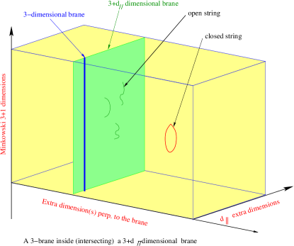
Figure 1: Geometrical representation of models with localized fermions.

2 MINIMAL MODELS WITH LOCALIZED FERMIONS

In a pictorial way, gravitons and SM particles can be represented as in Fig. 1. In particular, in the scenario we consider:

• the gravitons, depicted as closed strings, are seen to propagate in the whole higher-dimensional space, 3+$d_{\parallel}$+$d_{\perp}$. Here, 3+$d_{\parallel}$ defines the longitudinal dimension of the big brane drawn in Fig. 1, which contains the small 3-dimensional brane where the observed SM particles live. The symbol $d_{\perp}$ indicates instead the extra-dimensions, transverse to the big brane, which are felt only by gravity.

• The SM gauge-bosons, drawn as open strings, can propagate only on the (3+$d_{\parallel}$)-brane.

• The SM fermions are localized on the 3-dimensional brane, which intersects the (3+$d_{\parallel}$)-dimensional one. They do not propagate on extra-dimensions (neither $d_{\parallel}$ nor $d_{\perp}$), hence they do not have KK-excitations.

The number of extra-dimensions, $D=d_{\parallel}$,$d_{\perp}$ or $d_{\parallel}$+$d_{\perp}$, which are compactified on a $D$-dimensional torus of volume $V=(2\pi)^{D}R_{1}R_{2}\cdots R_{D}$, can be as big as six [404] or seven [405] dimensions. Assuming periodic conditions on the wave functions along each compact direction, the states propagating in the $(4+D)$-dimensional space are seen from the four-dimensional point of view as a tower of states having a squared mass:

$$M^{2}_{KK}\equiv M^{2}_{\vec{n}}=m_{0}^{2}+\frac{n_{1}^{2}}{R_{1}^{2}}+\frac{n_{2}^{2}}{R_{2}^{2}}+\cdots+\frac{n_{D}^{2}}{R_{D}^{2}}\,,$$ (1)

with $m_{0}$ the four-dimensional mass and $n_{i}$ non-negative integers. The states with $\sum_{i}n_{i}\neq 0$ are called KK-states. Assuming that leptons and quarks are localized is quite a distinctive feature of this class of models, giving rise to well defined predictions. An immediate consequence of the localization is that fermion interactions do not preserve the momenta in the extra-dimensions. One can thus produce single KK-excitations, for example via $f\bar{f^{\prime}}\rightarrow V_{KK}^{(n)}$ where $f,f^{\prime}$ are fermions and $V_{KK}^{(n)}$ represents massive KK-excitations of $W,Z,\gamma,g$ gauge-bosons. Conversely, gauge-boson interactions conserve the internal momenta, making the self-interactions of the kind $VV\rightarrow V_{KK}^{(n)}$ forbidden. The experimental bounds on KK-particles that we summarize in the following, as well as the discovery potential of the LHC, depend very sensitively on the assumptions made.

Electroweak measurements can place significant limits on the size of the extra-dimensions. KK-excitations might affect low-energy observables through loops. Their mass can thus be constrained by fits to the electroweak precision data [406, 344, 342, 407, 408, 409, 410]. In particular, the fit to the measured values of $M_{W}$, $\Gamma_{ll}$ and $\Gamma_{had}$ has led to $R^{-1}\geq$ 3.6 TeV.

3 WHAT CAN BE EXPECTED FROM THE LHC?

The possibility to produce gauge-boson KK-excitations at future colliders was first suggested in Ref. [401]. Unfortunately, from the above-mentioned limits, the discovery at the upgraded Tevatron is already excluded (see for instance [411]). Also expectations of a spectacular explosion of new resonances at the LHC are sorely disappointed. In the most optimistic case, the LHC will discover just the first excitation modes.

The only distinctive key from other possible non-standard models with new gauge-bosons would be the almost identical mass of the KK-resonances of all gauge bosons. Additional informations would be however needed to bring clear evidence for the higher-dimensional origin of the observed particle. Despite the interpretation difficulties, detecting a resonance would be of great impact.

We could also be in the less favorable case in which the mass of the KK-particles is bigger than the energy-scale probed at the LHC. In this unfortunate but likely scenario, the indirect effect of such particles would only consists in a slight increase of the events at high energies compared to the SM predictions. In this case, the luminosity plays a crucial role. In the last few years, several analysis have been performed in order to estimate the possible reach of the LHC (see for example [401, 411, 412, 413, 345, 414, 415, 416, 349]).

The three classes of processes where the new KK-resonances could be observed are:

• $pp\rightarrow l^{+}l^{-}$,

• $pp\rightarrow l\nu_{l}$, where $l\nu_{l}$ is for $l^{+}\nu_{l}+\bar{\nu}_{l}l^{-}$,

• $pp\rightarrow q\bar{q}$, where $q=u,d,s,c,b$.

The first class can be mediated by the KK-excitations of the electroweak neutral gauge-bosons, $Z_{KK}^{(n)}$ and $\gamma_{KK}^{(n)}$, while the second one can contain the charged $W_{KK}^{(n)}$ gauge-boson modes. Finally, the third class can receive contributions from all electroweak gauge-bosons plus the KK-modes $g_{KK}^{(n)}$ of the gluons.

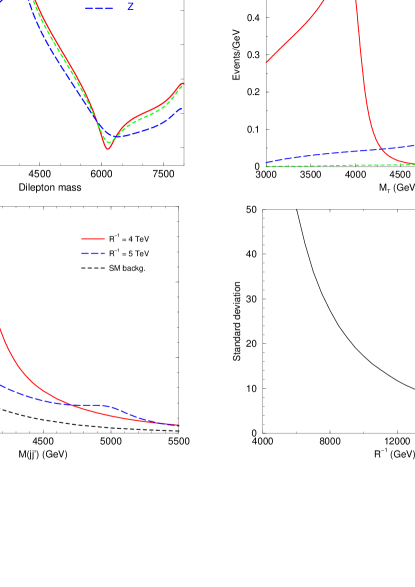
Figure 2: (a) Resonances of the first KK-excitation modes of $Z$ and $\gamma$ gauge-bosons. (b) Resonances of the first KK-excitation mode of the $W$-boson. (c) Resonances of the first KK-excitation mode of the gluon. (d) Under-hreshold effects due to the presence of $g_{KK}^{(n)}$, given in terms of the number of standard deviations from the SM predictions. The results have been obtained for the LHC with $\sqrt{s}$=14 TeV and L=100 fb^-1.

Typically, one can expect a kind of signal as given in Fig. 2. In the case where both outgoing particles are visible, a natural observable is the invariant mass of the fermion pair. Distributions in such a variable are shown in the upper and lower left-side plots, which display the interplay between $Z_{KK}^{(n)}$ and $\gamma_{KK}^{(n)}$ resonances, and the peaking structure due to $g_{KK}^{(n)}$, respectively. In presence of a neutrino in the final state, one can resort to the transverse mass distribution in order to detect new resonances. This is shown in the upper right-side plot of Fig. 2 for the charged-current process with $W_{KK}^{(n)}$ exchange. Owing to the PDFs, the effective center-of-mass (CM) energy of the partonic processes available at the LHC is not really high. The discovery limits of the KK-resonances are thus rather modest, $R^{-1}\leq$ 5-6 TeV. This estimate finds confirmation in more detailed ATLAS and CMS analyses [417]. Taking into account the present experimental bounds, there is no much space left. Moreover, the resonances due to the gluon excitations have quite large widths owing to the strong coupling value. They are thus spread and difficult to detect already for compactification scales of the order of 5 TeV.

But, what represents a weakness in this context can become important for indirect searches. The large width, ranging between the order of a few hundreds GeV for the KK-excitations of the electroweak gauge-bosons and the TeV-order for the KK-modes of the gluons, can give rise to sizeable effects even if the mass of the new particles is larger than the typical CM-energy available at the LHC. This is illustrated in the lower right-side plot of Fig. 2, where the number of standard deviations quantifies the discrepancy with the SM predictions, coming from $g_{KK}^{(n)}$ contributions. The under-threshold effects are driven by the tail of the broad Breit-Wigner, which can extend over a region of several TeV, and are dominated by the interference between SM and KK amplitudes. They thus require to have non-suppressed SM contributions. Their size, of a few-per-cent order for large compactification radii, can become statistically significant according to the available luminosity. In the extreme case of Fig. 2, we have a KK-gluon with mass $M_{1}=R^{-1}$=20 TeV and width $\Gamma_{1}\simeq$2 TeV. Assuming a luminosity L=100$fb^{-1}$, the interference terms give rise to an excess of about 2000 events. Similar conclusions hold for the indirect search of the KK-excitations of the electroweak gauge-bosons. At 95% confidence level, the LHC could exclude values of compactification scales up to 12 and 14 TeV from the $Z_{KK}^{(n)}+\gamma_{KK}^{(n)}$ and $W_{KK}^{(n)}$ channels, respectively. The indirect search is exploited in the ATLAS and CMS joint analysis of Ref. [417].

4 GOING BEYOND MINIMAL

We have carried the discussion above for the case of one extra-dimension with all fermions localized on the boundaries. One can depart from this simple situation in many ways:

• More extra-dimensions

  New difficulties arise for $D\geq 2$: the sum over KK propagators diverges [399]. A simple regularization is to cut off the sum of the KK states at $M_{s}$. This would be natural if the extra-dimension were discrete, however in our model we assumed translation invariance of the background geometry (before localizing any objects in it). String theory seems to choose a different regularization [399, 418]. In fact the interaction of $A^{\mu}(x,\vec{y})=\sum_{{\vec{n}}}{\cal A}^{\mu}_{\vec{n}}(x)\exp{i\frac{n_{i}y_{i}}{R_{i}}}$ with the current density $j_{\mu}(x)$, associated to the massless localized fermions, is described by the effective Lagrangian:

  $$\int d^{4}x\,\,\,\,\sum_{{\vec{n}}}e^{-\ln{\delta}\sum_{i}\frac{n_{i}^{2}l_{s}^{2}}{2R_{i}^{2}}}\,\,\,\,\,j_{\mu}(x)\,{\cal A}^{\mu}_{\vec{n}}(x)\,,$$ (2)

  which can be written after Fourier transformation as

  $$\int d^{4}y\,\int d^{4}x\,\,\,\,(\frac{1}{l_{s}^{2}2\pi\ln{\delta}})^{2}e^{-\frac{{\vec{y}}^{2}}{2l_{s}^{2}\ln{\delta}}}\,j_{\mu}(x)\,A^{\mu}(x,\vec{y})\,.$$ (3)

  This means that the localized fermions are felt as a Gaussian distribution of charge $e^{-\frac{{\vec{y}}^{2}}{2\sigma^{2}}}j_{\mu}(x)$ with a width $\sigma=\sqrt{\ln{\delta}}\,l_{s}\sim 1.66\,l_{s}$. Here we used $\delta=16$ corresponding to a $Z_{2}$ orbifolding. The couplings of the massive KK-excitations to the localized fermions are then given by:

  $$g_{{\vec{n}}}={\sqrt{2}}\sum_{{\vec{n}}}e^{-\ln{\delta}\sum_{i}\frac{n_{i}^{2}l_{s}^{2}}{2R_{i}^{2}}}g_{0}$$ (4)

  where the factor ${\sqrt{2}}$ stands for the relative normalization of the massive KK wave function ($\cos(\frac{n_{i}y_{i}}{R_{i}})$) with respect to the zero mode, and $g_{0}$ represents the coupling of the corresponding SM gauge-boson.

  The amplitudes depend on both $R$ and $M_{s}$ and thus, as phenomenological consequence, all bounds depend on both parameters (see [411]).

• Localized kinetic and/or mass terms for bulk fields

  Let us denote by $S_{0}(p,R,M_{s})$ the sum of all tree-level boson propagators weighted by a factor $\delta^{-\frac{{\vec{n}}^{2}}{R^{2}M_{s}^{2}}}$ from the interaction vertices. For simplicity we take $m_{0}=0$, and define $\delta S_{0}$ by

  $$S_{0}(p,R,M_{s})=\frac{1}{p^{2}}+\delta S_{0}\ .$$ (5)

  In order to confront the theory with experiment, it is necessary to include a certain number of corrections. The obvious one is a resummation of one-loop self-energy correction to reproduce the gauge coupling of the massless vector-bosons. Here we parametrize these effects as two kinds of bubbles to be resummed:

  • the first, denoted as ${\cal B}_{bulk}$ represents the bulk corrections. This bubble preserves the KK-momentum,

  • the second, denoted as ${\cal B}_{bdary}$ represents the boundary corrections. This bubble does not preserve the KK momentum. In fact, this can represent a boundary mass term or tree-level coupling, but also localized one-loop corrections due to boundary states [399] or induced by bulk states themselves [419].

  Here, two simplifications have been made: (a) the corrections are the same for all KK-states, and (b) the boundary corrections arise all from the same boundary. This results in the corrected propagator [399]:

  $$S_{corr}(p,R,M_{s})=\frac{S_{0}}{1-{\cal B}_{bulk}-{\cal B}_{bdary}-p^{2}\delta S_{0}{\cal B}_{bdary}}\ .$$ (6)

  If we define the “renormalized coupling” as $g^{2}(p^{2})=\frac{g^{2}}{1-{\cal B}_{bulk}-{\cal B}_{bdary}}$, the result is

  $$g^{2}S_{corr}=g^{2}(p^{2})S_{0}-\delta S_{0}\frac{g^{2}(1-p^{2}\delta S_{0}){\cal B}_{bdary}}{(1-{\cal B}_{bulk}-{\cal B}_{bdary})(1-{\cal B}_{bulk}-{\cal B}_{bdary}p^{2}\delta S_{0})}\ .$$ (7)

  The first term in Eq.(7) is the contribution that was taken into account in all phenomenological analysis, the second is the correction which depends crucially on the size of ${\cal B}_{bdary}$.

• Spreading interactions in the extra dimensions

  In the simplest scenario, all SM gauge-bosons propagate in the same compact space. However, one may think that the three factors of the SM gauge-group can arise from different branes, extended in different compact directions. In this case, $d_{\parallel}$ TeV-dimensions might be longitudinal to some brane and transverse to others. As a result, only some of the gauge-bosons can exhibit KK-excitations. Such a framework is discussed in [411].

These are simplest extensions of the work we presented above. The experimental limits depend now on many parameters $M_{s},{\cal B}_{bdary},...$ in addition to the different size of the compactification space felt by the gauge-bosons.

Part 25 Kaluza–Klein dark matter: a review

G. Servant

1 INTRODUCTION

The dominant matter component of our Universe is non-baryonic. The recently published WMAP results [3], combined with ACBAR, CBI and 2dFGRS, lead to precise estimates of the baryonic, matter and total densities : $\Omega_{b}h^{2}=0.0224\pm 0.0009$, $\Omega_{m}h^{2}=0.135\pm 0.009$ and $\Omega_{tot}=1.02\pm 0.02$. One of the most interesting aspects of the dark matter puzzle is that it is likely to be related to new physics at the TeV scale. Indeed, particles with weak scale size interactions and a mass at the electroweak breaking scale (WIMPs) are typically predicted to have the good relic density today to account for dark matter, provided that they are stable. The favorite WIMP candidate to date is the Lightest Supersymmetric Particle (LSP) and neutralinos are certainly the most extensively studied example.

2 DARK MATTER CANDIDATES FROM EXTRA DIMENSIONS

Alternative models for physics beyond the Standard Model (SM) that make use of extra dimensions rather than supersymmetry to solve the gauge hierarchy problem, have been studied in the last few years. It is now legitimate to ask whether extra dimensions have anything to do with the dark matter puzzle. Among the new ingredients of extra dimensional theories are the Kaluza-Klein (KK) excitations of SM particles as well as the radion, the scalar degree of freedom related to the size of extra dimensions. If the extra-dimensional model contains branes, there are also possibly branons, which are associated to brane fluctuations. All of them look like natural candidates for dark matter. Let us start with KK particles. The idea that they could form the dark matter is very tempting. However, it turns out that this is not so easy to achieve. Indeed, in most extra-dimensional models, there are no stable KK states, all being able to decay into SM particles. So the next question is: What are the new symmetries available in extra dimensional contexts which could make a KK mode stable? A new dimension means a new conserved momentum along the extra dimension. This leads to the so-called KK parity, a discrete symmetry which remains unbroken in some specific class of extra dimensional models named Universal Extra Dimensions (UED) [314]. As a result, the Lightest KK particle (LKP) is stable. We can also ask whether there is anything comparable to what happens with supersymmetric dark matter. In this case, the symmetry which guarantees the stability of the LSP has been primarily postulated to get rid of the proton decay problem in the MSSM. The proton decay problem arises also in extra dimensional theories specifically if the cut-off scale is near the TeV scale. It is interesting to investigate whether the symmetry one assumes to get rid of the proton decay can lead to a stable particle, like in susy. We will indeed present such solution in the context of warped GUT models where the DM particle is called the LZP. The LKP and the LZP are presently the two main proposals for WIMP KK dark matter. We will present them in more detail in the next sections. Before doing that, let us review other (non-wimp) possibilities which have been mentioned in the literature.

For a particle to be stable, either it has large couplings to SM particles and there must be a symmetry to guarantee its stability– this is the case of wimps like the LSP, the LKP and the LZP which will be presented below– or it interacts so weakly that its lifetime is longer than the age of the universe, this is the case of light particles with only gravitational couplings like the radion in ADD [403] or TeV flat extra dimensions. We go through the various possibilities in the next subsections. The situation is summarized in Table 1.

		$\bullet$ radion dark matter $m\sim$ meV
ADD models	only gravity in bulk	$\bullet$ KK graviton dark matter $m\sim$ meV
$R\sim$ meV-1 (flat)		(both finely-tuned)
		$\bullet$ branon dark matter
		(not original ADD, hierarchy pbs remain)
	$\rightarrow$ gauge bosons in bulk	$\bullet$ radion dark matter $m\sim$ meV
TeV-1 dim.		(finely-tuned); KK graviton is unstable
$R\sim$ TeV-1 (flat)
		$\bullet$ radion dark matter $m\sim$ meV
	$\rightarrow$ all SM fields in bulk	(finely-tuned)
	“Universal Extra Dimensions”	$\bullet$ KK dark matter $m\sim$ TeV
		$\rightarrow$ WIMP or SuperWIMP
	AdS a la Randall-Sundrum	$\bullet$ radion is unstable
Warped
geometries	if GUT in the bulk   $\longrightarrow$	$\bullet$ KK dark matter
$R\sim M_{Pl}^{-1}$		$m\sim$ few GeV–few TeV
but $M_{KK}\sim$ TeV		$\rightarrow$ WIMP

Table 1: Dark matter candidates in three main classes of extra dimensional models

2.1 KK graviton

2.1.1 In ADD

The KK graviton of ADD, with a meV mass, is stable on cosmological scales (each KK graviton couples only with $1/M_{Pl}$) and could be a DM candidate. It would not be a wimp and the correct relic density cannot be obtained via the standard thermal calculation. To get the correct relic density requires fine-tuning either in initial conditions for inflation or in the reheat temperature of the universe, otherwise, KK gravitons would overclose the universe. In addition, there are strong astrophysical constraints on the ADD scenario.

2.1.2 In UED: SuperWIMP KK graviton

The situation is different in UED models where the right relic abundance can be obtained naturally. The idea is that the standard cold relic abundance is obtained for the next lightest KK particle (NLKP), which is a WIMP (a KK hypercharge gauge boson in UED with $\sim$TeV mass) and the NLKP later decays into the LKP which is the KK graviton. That way, the KK graviton, which has a TeV mass and only a gravitational coupling can still acquire the right abundance as given by the standard thermal relic calculation. This scenario has been intensively studied by Feng et al [420, 421, 422].

Finally, let us mention that in Randall-Sundrum models, KK gravitons have a TeV mass and interact strongly so they cannot play the role of dark matter.

2.2 Radion

The radion in ADD has typically the same mass and same coupling as the KK graviton and also suffers from an overclosure problem. As for models with TeV extra dimensions, there is also typically an overclosure problem. Solving it requires modifying the assumptions on the compactification scheme. Details of radion cosmology have been studied in [423]. The radion overclosure problem does not apply in Randall-Sundrum where the radion has large interactions and large mass so that it decays fast.

2.3 Branons

Branons correspond to brane fluctuations. They control the coordinate position of our brane in the extra dimensions.Those fields can be understood as the goldstone boson arising from spontaneous breaking of translational invariance by the presence of the brane. They get massive by the explicit breaking of the symmetry. The possibility that branons could be dark matter has been investigated in [424, 425]. In this context, the SM lives on a 3D brane embedded in a higher dimensional (D=4+N) space-time where the fundamental scale of gravity $M_{D}$ is lower than the Planck scale. In the original ADD proposal, $M_{D}$ was the TeV scale. The authors of branon dark matter work in a general brane world scenario with arbitrary fundamental scale (larger than the TeV scale). The branon degree of freedom cannot be neglected when the brane tension scale $f$ is much smaller than $M_{D}$, which means that we live on a non rigid brane. Branon interactions with particles living on the brane can be computed as a function of $f$, $N$ and the branon mass $M$. Couplings of KK modes to the fields confined on the brane are exponentially suppressed by the fluctuation of the brane [426]. As $f$ is very small, the KK mode contributions become invisible from our world and the only remaining degrees of freedom are the branons. The gravitational interaction on the brane conserves parity and terms in the effective Lagrangian with an odd number of branons are forbidden. As a consequence, branons are stable. Constraints in the region of parameters made by $N$, $M_{D}$, $M$ and $f$ have been derived. We refer the reader to [424, 425] for details and references.

2.4 KK “photon”

As it will be presented in the next section, in the class of models with Universal Extra Dimensions [314], the Lightest KK Particle (LKP) is stable. For $\sim$TeV^-1 sized extra dimensions, the LKP can act as a WIMP. It was identified as the first KK excitation of the photon. To be precise, it is not really a KK photon because the Weinberg angle for KK modes is very small [348]. It is essentially the KK hypercharge gauge boson: $B^{(1)}$. Relic density [381, 427, 428, 380, 392], direct [391, 429] and indirect detection [391, 430, 431, 432, 433, 434, 435] studies of this candidate have all been carried out in the last few years. Constraints on these models from radion cosmology have also been studied [423].

2.5 KK neutrino

The possibility that the LKP is a KK $\nu_{L}$ rather than a KK photon in UED was also studied in [381, 429]. This case is excluded experimentally by direct detection experiments because of the large coupling of $\nu_{L}^{(1)}$ to the Z gauge boson, leading to much too large elastic scattering of the KK neutrino with nucleons.

It could also be that the LKP is the KK excitation of a RH neutrino. To behave as a WIMP, such particle should interact with TeV KK gauge bosons like in Left Right gauge theories such as Pati-Salam or $SO(10)$. This possibility was investigated in details in the context of warped geometries and more specifically in the context of warped Grand Unified Theories (GUTs) [436, 382]. It will be presented in section 4.

To summarize, so far, KK particles arise as stable viable WIMPs in two frameworks : In Universal Extra Dimensions and in some warped geometries à la Randall-Sundrum. We will discuss these two possibilities in more details now.

3 THE LKP IN UNIVERSAL EXTRA DIMENSIONS

In models with Universal Extra Dimensions (UED) [314] which are explained earlier in these proceedings, all SM fields propagate in flat toroidal extra dimensions, unlike models with Large Extra Dimensions à la ADD. Translation invariance along an extra dimension is only broken by the orbifold imposed to recover a chiral SM spectrum. Still, there is a remnant discrete symmetry called KK parity, $(-1)^{n}$, where $n$ is the KK number. This symmetry insures that interaction vertices cannot involve an odd number of odd-KK states and, therefore, a vertex with two SM particles (with $n=0$) and one KK state (with $n=1$) is forbidden. As a result, the Lightest KK Particle (LKP) with $n=1$ cannot decay into SM particles and is stable. Note that for KK parity to be an exact symmetry, one has to assume that the boundary lagrangians at the two orbifold fixed points are symmetric.

In contrast with supersymmetry where the mass spectrum is largely spread so that at most a few additional particles participate in coannihilation processes with the LSP, in Minimal UED (MUED), the mass spectrum of KK particles is rather degenerate and there are many coannihilation processes. The KK mass splittings are essentially due to radiative corrections. Those were computed in [348]. The spectrum of KK masses depends also on the values of boundary terms at the cut-off scale, which are not fixed by known SM physics. In this sense, the values of the KK masses can be taken arbitrary and the UED scenario has a multitude of parameters. The authors of [348] assumed that the boundary terms vanish (this is the so-called MUED hypothesis). In this case, the LKP is the KK hypercharge gauge boson $B^{(1)}$.

The viability and relic density of the LKP were first analyzed in [381] with some simplifying assumption about the KK spectrum. Only one co-annihilation channel was considered (involving the KK right-handed electron). Ref. [380, 392] include all coannihilation channels with KK fermions and KK gauge bosons and look at the effect of each channel separately. The net result is that even if the new coannihilations are Boltzmann suppressed their effect is still significant because the cross sections are mediated by weak or strong interactions while the cross sections studied so far were purely hypercharge-mediated processes. Their conclusion is that in MUED, the LKP mass should be within 500-600 GeV while in non-minimal UED models, freedom in the KK mass spectrum allows an LKP as heavy as 2 TeV. For an analysis taking into account the effects of second level KK modes see [427, 428]. The effect of coannihilation with the KK Higgs was studied in [437]. Shortly after the appearance of [380, 392], Ref. [438] came out where they derive a strong constraint on the KK scale of MUED models from precision EW observables ($>$ 700 GeV). This seems to exclude MUED KK dark matter but KK dark matter survives in non-minimal UED models, where the KK mass can be as large as 2 TeV.

To conclude this section, note that the cases where the LKP is a KK $Z$ or KK $H$ remain to be analysed. The interesting D=6 case has not been investigated either. We refer to the proceedings by B. Dobrescu for references on the collider phenomenology of UED. We now move to direct detection constraints.

3.1 Direct and indirect detection

Direct detection of the $B^{(1)}$ LKP has been studied in germanium, sodium iodine and xenon detectors [429, 391]. It does not appear as the most promising way to probe $B^{(1)}$ dark matter as is summarized in fig.2.

Figure 1: Leading Feynman graphs for effective $B^{(1)}$-quark scattering through the exchange of a KK quark (both $q^{(1)}_{L}$ and $q^{(1)}_{R}$) and through the exchange of a zero-mode Higgs boson.

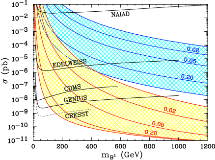
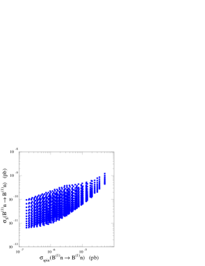
Figure 2: Left figure is from [391]: Predicted spin-dependent (dark-shaded, blue) and spin-independent (light-shaded, red) proton cross sections. The predictions are for $m_{h}=120$ Gev and $0.01\leq\Delta=(m_{q^{1}}-m_{B^{1}})/m_{B^{1}}\leq 0.5$, with contours for specific intermediate $\Delta$ labeled. Right figure is from [429]: Predictions for $B^{(1)}$-nucleon cross sections in the spin-dependent – spin-independent plane where three parameters are varied: $m_{B^{(1)}}$ in the 600-1200 GeV range, $\Delta$ in the 5-15 $\%$ range and $m_{h}$ in the 100-200 GeV range. We cannot expect a spin-independent cross section larger than $10^{-9}$ pb if we remain in this most likely region of parameter space.

Indirect detection through gamma-rays [391, 431, 433, 434, 435], neutrinos and synchrotron flux [431], positrons [391, 432], antiprotons [443] or through antideuterons [444] has also been considered. The neutrino spectrum from LKP annihilation in the Sun was investigated in [432]. An interesting feature of KK dark matter is, in constrast with the neutralino, that annihilation into fermions is not helicity suppressed and there can be a direct annihilation into $e^{+}e^{-}$ leading to a very valuable positron signal from LKP annihilation into the galactic halo [391].

4 THE LZP IN WARPED GUTS

The interest in the phenomenology of extra dimensions over the last few years has been motivated by the goal of understanding the weak scale. The only extra-dimensional geometry which really addresses the hierarchy problem is the Randall-Sundrum geometry. Particle physics model building in this framework has been flourishing and a favorite class of models has emerged: that where all SM fields propagate in the bulk of AdS₅, except for the Higgs (or alternative physics responsible for electroweak symmetry breaking) which is localized on the IR brane. In addition, the electroweak gauge group should be extended to $SU(2)_{L}\times SU(2)_{R}\times U(1)$. Those models were embedded into a GUT in Refs. [436, 382] and it is in this context that a viable dark matter appears: A stable KK fermion can arise as a consequence of imposing proton stability in a way very reminiscent to R-parity stabilizing the LSP in supersymmetric models. The symmetry is called $Z_{3}$ and is a linear combination of baryon number and $SU(3)$ color. As soon as baryon number is promoted to be a conserved quantum number, the following transformation becomes a symmetry:

$$\Phi\rightarrow e^{2\pi i\left(B-\frac{n_{c}-\bar{n}_{c}}{3}\right)}\Phi$$ (1)

where $B$ is baryon-number of a given field $\Phi$ (proton has baryon-number $+1$) and $n_{c}$ ($\bar{n}_{c}$) is its number of colors (anti-colors). This symmetry actually exists in the SM but SM particles are not charged under it since only colored particles carry baryon number in the SM. In Refs. [436, 382], and more generally in higher dimensional GUTs, baryon number can be assigned in such a way that there exists exotic KK states with the gauge quantum numbers of a lepton and which carry baryon number as well as KK quarks which carry non-standard baryon number. These particles carry a non-zero $Z_{3}$ charge. The lightest of these, called the Lightest $Z_{3}$ Particle (LZP), is stable since it cannot decay into SM particles.

So, who is the LZP? We recall that in extra-dimensional GUTs, there is a need for a replication of GUT multiplets to avoid fast proton decay. Zero modes (SM particles) come from different GUT multiplets. Consequently, in a given multiplet, there are KK modes without the corresponding zero-modes. The mass spectrum of KK fermions is determined by their bulk mass, called $c$ in Planck mass units, and the boundary conditions (BC) at the TeV and Planck brane. All KK modes of a given multiplet have the same $c$. The $c$ parameter also fixes the localization of the wave function of the zero modes. BC are commonly modelled by either Neumann ($+$) or Dirichlet ($-$) BC in orbifold compactifications. 5D fermions lead to two chiral fermions in 4D, one of which only gets a zero mode to reproduce the chiral SM fermion. SM fermions are associated with ($++$) BC (first sign is for Planck brane, second for TeV brane). The other chirality is ($--$) and does not have zero mode. In the particular case of the breaking of the grand unified gauge group to the SM, Dirichlet boundary conditions are assigned on the Planck brane for fermionic GUT partners which do not have zero modes, they have ($-+$) boundary conditions. When computing the KK spectrum of $(-+)$ fermions one finds that for $c<1/2$ the lightest KK fermion is lighter than the lightest KK gauge boson. For the particular case $c<-1/2$, the mass of this KK fermion is exponentially smaller than that of the gauge KK mode! Fig. 3 shows the mass of the lightest ($-+$) KK fermion as a function of $c$ and for different values of the KK gauge boson mass $M_{KK}$. There is an intuitive argument for the lightness of the KK fermion: for $c\ll 1/2$, the zero-mode of the fermion with $(++)$ boundary condition is localized near the TeV brane. Changing the boundary condition to $(-+)$ makes this “would-be” zero-mode massive, but since it is localized near the TeV brane, the effect of changing the boundary condition on the Planck brane is suppressed, resulting in a small mass for the would-be zero-mode.

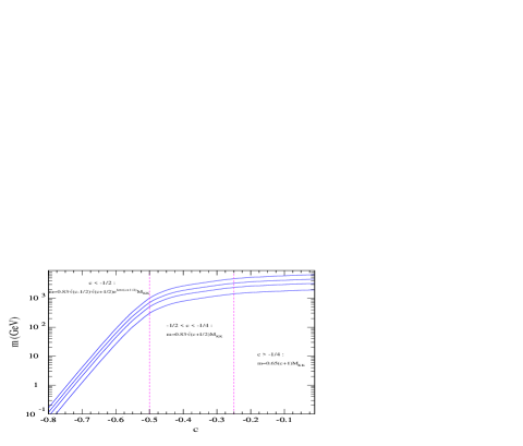
Figure 3: Mass of the lightest KK fermion as a function of its $c$ parameter for different values of the KK gauge boson mass. From bottom to top, $M_{KK}=$3, 5, 7, 10 TeV. For large and negative $c$, the KK fermion can be infinitely light. For KK fermions belonging to the GUT multiplet containing the RH top, $c\sim-1/2$.

We have just seen that in warped GUT models, there is not a single KK scale since the scale for KK fermions can be different from the scale of KK gauge bosons. Now, among the light KK fermions, the one which is the lightest is the one with the smallest $c$ parameter. This means that the lightest KK fermion will come from the GUT multiplet which contains the top quark. Indeed, the top quark, being the heaviest SM fermion, is the closest to the TeV brane. This is achieved by requiring a negative $c$. Thus, all $(-+)$ KK fermions in the GUT multiplet containing the SM top quark are potentially light. Mass splittings between KK GUT partners of the top quark can have various origins, in particular due to GUT breaking in the bulk as discussed in [436, 382]. There is large freedom here and the identification of the LZP comes from phenomenological arguments: Indeed, the only massive elementary Dirac fermion (with a mass in the 1 GeV - 1 TeV range) which could be a viable dark matter candidate is the neutrino. If such a neutrino had the same coupling to the $Z$ as in the SM, however, it would be excluded by direct detection experiments. Its coupling to the $Z$, therefore, must be suppressed. Thus, we are left with the possibility of a KK Right-Handed (RH) neutrino. In models where the electroweak gauge group is extended to $SU(2)_{L}\times SU(2)_{R}\times U(1)$, the RH neutrino has gauge interactions in particular with the additional $Z^{\prime}$. Nevertheless, its interactions with ordinary matter are feeble because they involve the additional gauge bosons which have a large mass ($M_{KK}\mathrel{\hbox to0.0pt{\lower 4.0pt\hbox{\hskip 1.0pt$\sim$}\hss}\raise 1.0pt\hbox{$>$}}3$ TeV). This opens the possibility of a weakly interacting Dirac RH neutrino. In principle, the LZP is not necessarily the lightest KK particle. There might be lighter KK modes but which are unstable because they are not charged under $Z_{3}$. In practise though, and in the models of [436, 382], the RH neutrino LZP turns out to be the lightest KK particle due to various phenomenological constraints.

In summary, the LZP is a Kaluza–Klein fermion, which is a four-component spinor and vector-like object. As explained in great detail in Ref. [382], it can be naturally very light, much lighter than the KK scale of Randall-Sundrum models, namely $M_{KK}\mathrel{\hbox to0.0pt{\lower 4.0pt\hbox{\hskip 1.0pt$\sim$}\hss}\raise 1.0pt\hbox{$>$}}$ 3 TeV. This is because the RH chirality is localized near the TeV brane while the LH one is near the Planck brane. The overlap of wave functions is small, resulting in a small Dirac KK mass. Its lightness is related to the top quark’s heaviness but not entirely fixed by it, so that LZPs in the mass range of approximately 20 GeV to a few TeV can be considered. We refer to the LZP as if it were a chiral fermion because only the RH chirality has significant interactions and the other chirality decouples. In addition, the LZP has the same gauge quantum numbers as the RH neutrino of $SO(10)$ or Pati–Salam. As a result, we refer to it as a “Dirac RH neutrino”.

Via the AdS/CFT correspondence, the Randall-Sundrum scenario is dual to a 4D composite Higgs scenario, in which the unification of gauge couplings has recently been studied [446]. In this case, the LZP maps to some low-lying hadron at the composite scale. We also point out that in Refs. [436, 382], the strong coupling scale is close to the curvature scale so that ${\cal O}(1)$ variations in calculations are expected. Results of [436, 382] should therefore be considered as representative rather than a complete description.

4.1 Relic Density

An interesting feature of warped GUT models is that GUT states such as $X,Y$ gauge bosons appear at the TeV scale (via the KK excitations). In $SO(10)$, there are also the $X^{\prime},Y^{\prime}$, $X_{s}$, $Z^{\prime}$, etc. that the LZP can couple to. The LZP couples to the TeV KK gauge bosons of $SO(10)$. In addition, when electroweak symmetry is broken, $Z-Z^{\prime}$ mixing induces a coupling of the RH neutrino to the SM $Z$ gauge boson. This coupling is suppressed by $(M_{Z}/M_{Z^{\prime}})^{2}$. If $M_{Z^{\prime}}\sim$ few TeV (the mass of KK gauge bosons is set by $M_{KK}$), the size of this coupling will typically be ideal for a WIMP. There is actually a second source for the $Z$-LZP coupling, which we will not discuss here but refer the reader to Ref. [382] for a detailed explanation. The point is that there is enough freedom in the model under consideration to treat the LZP-$Z$ coupling as an almost arbitrary parameter.

For LZPs lighter than approximately 100 GeV, LZP annihilations proceed dominantly via s-channel $Z$-exchange and annihilations to light quarks, neutrinos and charged leptons are important. For larger masses, annihilation via the t-channel exchange of $X_{s}$ into top quarks or via s-channel $Z^{\prime}$ exchange into $t\overline{t}$, $b\overline{b}$, $W^{+}W^{-}$ and $Zh$ dominates. LZPs can generate the observed quantity of dark matter thermally in two mass ranges: near the $Z$-resonance ($m_{\rm{LZP}}\approx$ 35-50 GeV) and for considerably heavier masses ($m_{\rm{LZP}}\mathrel{\hbox to0.0pt{\lower 4.0pt\hbox{\hskip 1.0pt$\sim$}\hss}\raise 1.0pt\hbox{$>$}}$ several hundred GeV) [436, 382]. Several approximations were made in the relic density calculation of [436, 382], like using the non-relativistic expansion, neglecting the annihilation via s-channel Higgs exchange as well as co-annihilation with KK $\tau^{\prime}_{R}$ . A more precise calculation is being carried out using the COMPHEP model for warped GUTs and associated with MICROMEGAS [447].

Annihilations can vary from one Dirac RH neutrino dark matter model to another, depending on whether, at large LZP mass, annihilations take place via s-channel $Z^{\prime}$ exchange only or also via a t-channel $X_{s}$–type gauge boson. On the other hand, the elastic scattering cross section is mainly model-independent (determined by the LZP -$Z$ coupling).

4.2 Direct and indirect Detection

Concerning elastic scattering, as is well-known for a Dirac neutrino, the spin independent elastic scattering cross section via a t-channel Z exchange has the form

$$\sigma_{SI}\propto\left[Z(1-4\sin^{2}\theta_{\rm{W}})-(A-Z)\right]^{2}.$$ (2)

Since $4\sin^{2}\theta_{\rm{W}}\approx 1$, the coupling to protons is suppressed. Nevertheless, scattering off target nuclei puts the strongest constraints on the $M_{KK}$ scale. As reported in [436, 382], the prospects for LZP direct detection are extremely good and we expect that all the interesting region of parameter space in this model will be probed by near future direct detection experiments.

Indirect detection prospects for the LZP have been studied through three channels in [448]: First, the prospects for detecting high-energy neutrinos produced through annihilations of LZPs in the Sun are very encouraging. Annihilations of light LZPs in the Galactic Halo also generate positrons very efficiently. Finally, LZP annihilations near the Galactic center may provide an observable flux of gamma-rays not considerably different than for the case of annihilating neutralinos. [443] also studied the production of antiprotons from LZP annihilations and [444] looked at antideuteron fluxes.

4.3 Collider searches

The literature on warped phenomenology so far has dealt with a single KK scale $\mathrel{\hbox to0.0pt{\lower 4.0pt\hbox{\hskip 1.0pt$\sim$}\hss}\raise 1.0pt\hbox{$>$}}$ 3 TeV, making it difficult to observe KK states in RS at high-energy colliders. This is because most of the work on the phenomenology of Randall-Sundrum geometries have focused on a certain type of boundary conditions for fermionic fields. In section 15 of [436, 382], we emphasize the interesting consequences for collider phenomenology of boundary conditions which do not lead to zero modes but on the other hand may lead to very light observable Kaluza-Klein states. It is clear that in the models of [436, 382], all the KK states in the GUT multiplet containing the top quark can be very light thus can be produced at Tevatron or LHC. Something very interesting in this model is the multi $W$ final state which can be produced with a large cross section (as illustrated in Fig. 4). Some processes can lead to 6 $W$’s in the final state. A COMPHEP code for this model has been written to generate these processes and will soon become available. LHC prospects for some of these signatures are being studied [449].

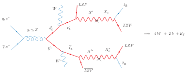
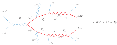
Figure 4: Production of KK quark $b^{\prime}_{L}$ and KK lepton $\tau^{\prime}_{L}$.

5 COMPARISONS BETWEEN THE LSP, LKP ad LZP

Table 2 gives a brief comparison of the LSP, LKP and LZP. For a more detailed comparison, see the last section of [448].

	LKP	LZP	LSP
Set up	Universal Extra Dimensions	Warped GUTs	SUSY
Nature of	Gauge boson	Dirac fermion	Majorana fermion
dark matter particle
	KK parity: consequence of	$Z_{3}$: imposed	R-parity: imposed
Symmetry	geometry if ones assumes	to protect	to protect
	equal boundary lagrangians	proton stability	proton stability
	${(-1)}^{n}$	$\displaystyle B-\frac{n_{c}-\overline{n}_{c}}{3}$	${(-1)}^{3(B-L)+2S}$
Mass range	$\sim$ 600-1000 GeV	20 GeV-few TeV	$\sim$ 50 GeV-1 TeV
Annihilation cross	s-wave	s-wave	p-wave
section into fermions			helicity-suppressed
Favourite detection	$\bullet$LHC	$\bullet$Direct detection	$\bullet$LHC
	$\bullet$Indirect detection	$\bullet$LHC
		$\bullet$Indirect detection

Table 2: Comparison between the wimp dark matter candidates discussed in this review.

6 CONCLUSION

Alternatives to SUSY dark matter exist and viable examples arise from extra dimensional models. Because of their simplicity, models with Universal Extra Dimensions have attracted much attention. The Minimal UED (MUED) model is an ideal benchmark model and a good starting point as far as the testability of extra dimensional models is concerned. Discriminating between MUED and SUSY at colliders is an active field of study. Most of the interest in UED is due to the possibility of a stable KK particle and in particular to the LKP as dark matter. Direct and indirect detection of the LKP have been investigated. On the other hand, UED do not particularly solve the hierarchy problem. Extra dimensional models with warped geometry do so. Among the Randall-Sundrum realizations, those with the SM fields living in the bulk are the most appealing. In this framework, the EW sector is extended to $SU(2)_{L}\times SU(2)_{R}\times U(1)$. In this report, we have reviewed a GUT embedding of this gauge structure, which we believe leads to a very rich and peculiar phenomenology. For instance, it is possible that the symmetry imposed to prevent proton decay leads to a stable KK particle which can act as dark matter. Note that independently from the existence of a stable KK mode, warped GUTs possess interesting features and there is still a lot to be done as far as phenomenological exploration of RS models with SM in the bulk is concerned.

Part 26 The Higgs boson as a gauge field

G. Cacciapaglia

1 INTRODUCTION

In the Standard Model of particle physics, the breaking of the electroweak symmetry is generated by a scalar field, the Higgs. The minimal Higgs sector consists of a doublet of the weak SU(2)_L: a suitable potential for such scalar will induce a vacuum expectation value for it that will break the gauge symmetry and give a mass both to the weak gauge bosons, the $W$ and $Z$, and to the matter fermions. This description is very successful from the experimental point of view: even though we do not have direct measurements in this sector, precision tests of the SM seem to be consistent with the presence of a relatively light Higgs, with mass between $115$ GeV and $\sim 300$ GeV. The lower bound comes from direct searches at LEP, while the upper bound comes from the loop effects of the Higgs to precision observables [450].

Notwithstanding this success, the Higgs mechanism is still unsatisfactory from a theoretical point of view. First of all, the potential is somehow put by hand and is not calculable for the Higgs boson is not protected by any symmetry. Moreover, from an effective theory point of view, the potential is unstable: loop corrections will induce a dependence on some new physics that appears at high energies. For instance, the mass term is quadratically sensitive to such new physics scale: the bounds on the Higgs mass would require this scale to be around $1$ TeV. This scale is much lower that the expected UV scales, like the Planck mass where quantum gravity becomes relevant, at $10^{16}$ TeV, or Grand Unification scales, around $10^{11}\div 10^{13}$ TeV. Unless a huge fine tuning is advocated, the SM contains a hierarchy between such scales. Moreover, building a model with new physics at a TeV is very difficult, because of bounds coming from precision observables: higher order operators, that will generically be generated by such new physics, pose a bound on the new physics scale around $5\div 10$ TeV  [451].

A very appealing idea, utilizing extra dimensions, is to identify the Higgs boson as the component along some extra spatial dimension of a gauge boson, and it was first proposed in Refs. [452, 453, 454]. In this way, the symmetry breaking does not come from a fundamental scalar of the theory, thus improving the stability of the mechanism. Moreover, gauge invariance in the extra dimensional theory will highly constrain the potential, forbidding for instance a mass term. Now, the loop contributions to the mass term will be insensitive to the cutoff of the theory, thus to the UV physics, and they may be responsible for EWSB. The crucial point here is that such contributions are finite and calculable! Due to gauge invariance itself, the EW scale will also be protected with respect to the UV cutoff. The simplest possibility is to work in 5 dimensions: in this case there is only one extra component

$$A_{M}=(A_{\mu},A_{5})\,.$$ (1)

The minimal requirements on the bulk gauge group $\mathcal{G}$ is that it has to contain the SM gauge group $\mathcal{G}\in$ SU(2)${}_{L}\times$U(1)_Y, and a doublet of SU(2)_L, to be identified with the Higgs, is embedded in the adjoint representation. The gauge group $\mathcal{G}$ is broken by an orbifold projection to the SM one $\mathcal{H}$ assigning different parities (or boundary conditions) to the gauge bosons of different generators. This corresponds to 

$$\begin{array}[]{rl}A^{a}_{\mu}(-y)=A^{a}_{\mu}(y)&\mbox{if}\,a\in\mathcal{H}\,,\\ A^{b}_{\mu}(-y)=-A^{b}_{\mu}(y)&\mbox{if}\,b\in\mathcal{G}/\mathcal{H}\,.\end{array}$$ (2)

For the $A_{5}$ component, 5D Lorentz invariance imposes opposite parities. Thus, there is a zero mode only along the broken generators: these are the only physical scalars in the spectrum, as all the massive modes of $A_{5}$ can be gauged away, and will play the role of the longitudinal modes of the massive vector bosons. In other words, the Higgs doublet has to be contained in $A_{5}^{b}$. The gauge transformations, at linear level, reads:

$$A_{\mu}\rightarrow A_{\mu}+\partial_{\mu}\lambda(x,x_{5})+i[\lambda(x,x_{5}),A_{\mu}]\,,$$ (3)

$$A_{5}\rightarrow A_{5}+\partial_{5}\lambda(x,x_{5})+i[\lambda(x,x_{5}),A_{5}]\,.$$ (4)

This symmetry is enough to ensure that it is not possible to write down a tree level potential for $A_{5}$ in the bulk. Indeed, the only invariant is the energy stress tensor

$$F_{MN}=\partial_{M}A_{N}-\partial_{N}A_{M}+ig[A_{M},A_{N}]\,;$$ (5)

being antisymmetric, $F_{55}=0$. The situation is more subtle on the fixed points of the orbifold: the gauge transformation parameter $\lambda$, has the same parities of the gauge fields $A_{\mu}$. Thus, for the broken generators, $\lambda$ is odd: this means that on the fixed point $x_{\star}$

$$A_{5}^{b}(x_{\star})\rightarrow A_{5}^{b}(x_{\star})+\partial_{5}\lambda^{b}(x_{\star}).$$ (6)

This incomplete gauge transformation, however, is enough to forbid a potential localized on the fixed points.

This argument can be generalized to more extra dimensions. The first difference is that a potential is allowed by gauge invariance: indeed, $F_{ij}$, where $i$ and $j$ are along the extra dimensions, is gauge invariant. In particular a quartic term may be generated at tree level. However, it is generically possible to write a linear term in the energy stress tensor on the fixed points: this will generate tadpoles for the scalars, so that one has to choose the orbifold projection in order to forbid them [456, 457].

While this mechanism offers great simplicity and elegance, building a realistic model is very difficult. The main problems are the lightness of the Higgs and of the top quark. Regarding the top, the Yukawas are generated via the gauge coupling itself, so it is generically hard to engineer a Yukawa of order 1 from a small gauge coupling. Regarding the Higgs mass, it turns out to be too small, below the value currently excluded by LEP, because the quartic scalar interaction term is generated at one loop. Since the entire potential (mass and quartic) is loop generated, the potential will also generically prefer large values of the Higgs vacuum expectation value (VEV) relative to the compactification scale so that the scale of new physics stays dangerously low. It is interesting to note that a deconstructed version of this mechanism [458] led to the idea of Little Higgs models. The symmetry protecting the Higgs mass is now a discrete shift symmetry, and the construction is much less constrained by the absence of 5D Lorentz invariance. In Little Higgs models, this idea has been pushed further: in this case the symmetry is protecting the Higgs mass at one loop, but allows a quartic coupling at tree level [459].

Several models, both in 5 (see Refs. [460, 461, 462, 463, 464, 465, 466]) and 6 (see Refs. [467, 468, 469]) dimensions have been proposed in the literature, in the context of flat extra dimensions. Another interesting development is to embed the same idea in a warped extra dimension [470] as in Refs. [471, 472, 446, 473]. The nice thing is that the warping enhances both the Higgs and top mass. However, the non trivial background will also induce corrections to electroweak precision observables that constitute the strongest constraint on this models. Interestingly, a correspondence fist developed in the string context allows to relate these theories to 4 dimensional ones, in particular to strongly coupled conformal theories (CFTs), where conformality is broken at the resonance scale. From this point of view, the Higgs is a composite particle of the CFT, like in the Georgi-Kaplan theories in Refs. [474, 475, 476, 477].

In the next sections we will briefly discuss the main features and differences of models in flat and warped space. For simplicity we will focus on two simple examples, nice for their simplicity and minimality: the SU(3)_w model in 5D of Ref. [463] in flat space, and the minimal composite Higgs model of Ref. [472]. However, the properties highlighted here are common to all the models proposed in the literature.

2 FLAT SPACE

As already mentioned above, we need to embed the SM electroweak gauge group, SU(2)${}_{L}\times$U(1)_Y, into a larger bulk gauge group, that contains a doublet of SU(2) in the adjoint representation. This group is broken to the SM one by an orbifold projection: in this way, at energies below the compactification scale, only the SM gauge symmetry is unbroken. A more general breaking of the symmetry can be achieved using boundary conditions: however in the following we will insist on the orbifold projection. The reason is the absence of tree level corrections to electroweak precision observables: in this case, a zero mode like the $W$ and $Z$ is orthogonal to all the massive KK modes of other fields. If the Higgs vev is constant along the extra dimension, as it is the case in flat space, it will not induce mixings between the zero modes and the KK modes: this is the source of universal corrections. If the symmetry breaking is not given by an orbifold parity, but by boundary conditions, the orthogonality argument does not work any more. We will comment more on this issue later.

The simplest choice is to enlarge the weak group to SU(3)_w, and break it to SU(2)${}_{L}\times$U(1)_Y on the orbifold $S^{1}/Z_{2}$: an analysis of all the rank 2 groups can be found in Ref. [468]. The adjoint of SU(3) decomposes into (3, 0) + (2, 1/2) + (2, -1/2) + (1, 0). After the orbifold projection, the only (massless) scalar left in the theory is a complex doublet with hypercharge $1/2$, that we identify with the SM Higgs $H_{5}$. As already mentioned, this scalar will not have any potential at tree level: however, loops will induce a potential that is insensitive to the UV cutoff, and thus calculable. For the moment we will assume that such potential will induce a VEV for the Higgs, thus breaking the electroweak symmetry. We can use SU(2) transformations to align the VEV, analogously to the SM case, and parametrize it

$$\langle H_{5}\rangle=\sqrt{2}\left(\begin{array}[]{c}0\\ \alpha/R\end{array}\right)\,.$$ (7)

It is now straightforward to compute the spectrum of the gauge bosons: we find

$$M_{Wn}=\frac{n+\alpha}{R}\,,\quad M_{Zn}=\frac{n+2\alpha}{R}\,,\quad M_{\gamma n}=\frac{n}{R}\,,$$ (8)

where $n\in Z$, and we want to identify the lightest state in each tower with the SM gauge bosons, the photon, the $W$ and the $Z$. Let us first point out that the spectrum is invariant if we shift $\alpha$ by an integer, and if we change its sign. In other words, the physical range for $\alpha$ is $[0,1/2]$ and all other vacua outside this range are equivalent, as the radiatively induced potential will respect the same symmetries. Another important feature is that $M_{Z}$ turns out to be twice the $W$ mass: this is a consequence of the gauge group SU(3) that predicts $\theta_{W}=\pi/3$. One possible way to fix it is to add localized gauge kinetic terms: SU(3) being broken on the boundaries, such terms can be different for the SU(2) and U(1) and, if large enough, can dominate and fix the correct value of $\sin\theta_{W}$. However, this scenario is equivalent to a warped extra dimension: integrating out a slice of the warped space near the Planck brane, where the warping is small, will mimic the localized kinetic terms, while the remaining space will be almost flat. We will discuss the warped case in the next section: the main drawback is that it suffers from tree level corrections to the precision observables [473]. Another possibility is to extend the gauge group with an extra U(1)_X. In this case, if the bulk fermions are charged, only the combination of the two U(1)’s proportional to the hypercharge is anomaly free, and the orthogonal gauge boson will develop a mass [467]. Alternatively, one can use boundary conditions to break U(1)${}_{w}\times$U(1)${}_{X}\to$ U(1)_Y, for instance by twisting the BC on one of the two branes, such that no zero mode is left in the scalar sector .

The next problem is how to generate a mass for the SM matter fields. If we added bulk fermions, with chiral zero modes thanks to the orbifold projection, the Higgs VEV would generate a spectrum similar to that in (8): all the light modes would have masses larger than the $W$ mass, where the exact relation depends on group theory factors arising from the fermion representations. Indeed, gauge invariance forces the Higgs to couple to bulk fields and with strength determined by the 5D gauge coupling $g_{5}$. There are two possible solutions: one is to include odd masses for these fermions, that will localize the zero modes toward the two fixed points. As modes with different chirality will be localized toward different points, this mechanism will reduce the overlaps between the wave functions, and generate hierarchies between the various Yukawa couplings. Another possibility, adopted in [468, 456] is to localize the SM fermions on the fixed points, and then mix them with massive bulk fields that will induce an effective Yukawa coupling a la Froggatt-Nielsen. In this case, the mass for the light fermions can be given either by small mixings, or by a large bulk mass that will exponentially suppress the effective Yukawa. In the latter case, with order 1 masses, it is possible to explain the hierarchies in the Yukawa sector [456, 466]. The flavour structure of the theory for the first two generations has been studied in Ref. [478].

The main problem in the fermion sector is then how to explain the heaviness of the top: indeed a bulk field will generically couple to the Higgs with the gauge coupling, predicting a fermion mass of order $m_{W}$. A possible way to fit the top is to embed it in a large representation, such that the effective Yukawa is enhanced by a group theory factor. This possibility has been exploited in Ref. [465]: the authors find that the minimal representation of SU(3)_w is a symmetric $\bf\bar{15}$. This choice would predict $m_{t}=2m_{W}$ at tree level: QCD corrections might enhance the pole mass to a realistic value. The main drawback of this possibility is that the largish representation will lower the scale where the extra dimensional theory becomes strongly coupled. For the $\bf\bar{1}5$, using Naive Dimensional Analysis, we can estimate such scale to $2\div 3\times 1/R$. Moreover, the presence of a triplet of SU(2) in the decomposition of the $\bf\bar{1}5$ will introduce tree level correction to the coupling of the $b_{l}$ with the $Z$. Such corrections come from the mixing with the zero mode of the triplet and not from the effect of the KK modes. Removing the zero mode with a localized mass will induce mixing with the KK modes: this corrections can be translated into a bound on the compactification scale $1/R>4\div 5$ TeV. Another possibility pursued in Ref. [466] is to explicitly break Lorentz invariance along the extra dimension. In this case, each fermion will effectively feel a different length, thus removing the relation between the top and the $W$ masses. The strong coupling scale is also lowered, but in a less dramatic way. However, in this case, the Lorentz breaking will induce a UV cutoff sensitivity in the Higgs potential at higher loop level. In Ref. [466] the authors focus their attention on the flavour problem: again corrections to $Zb_{l}\bar{b}_{l}$ and 4 fermion operators induced from the gauge boson resonances [407, 479] pose a bound on the scale $1/R$ of few TeV.

Once the field content in the bulk is specified, it is possible to compute the Higgs potential as it is finite. Their spectrum, as a function of the Higgs VEV $\alpha$, generically takes the form:

$$m_{n}^{2}=M^{2}+\frac{(n+\xi\alpha)^{2}}{R^{2}}\,,\quad n\in Z\,,$$ (9)

where $\xi$ is determined by the representation of the field. We can use the Higgs-dependent spectrum to compute the full one-loop potential, using the Coleman-Weinberg formula: after summing over the KK modes [467], we find

$$V_{eff}(\alpha)=\frac{\mp 1}{32\pi^{2}}\frac{1}{(\pi R)^{4}}\mathcal{F}_{\kappa}(\alpha)\,,$$ (10)

where the signs stand for bosons/fermions and

$$\mathcal{F}_{\kappa}(\alpha)=\frac{3}{2}\sum_{n=1}^{\infty}\frac{e^{-\kappa n}\cos(2\pi\xi\alpha n)}{n^{3}}\left(\frac{\kappa^{2}}{3}+\frac{\kappa}{n}+\frac{1}{n^{2}}\right)\,,$$ (11)

where $\kappa=2\pi MR$. The contribution of fields with large bulk mass is exponentially suppressed. Moreover, the leading contribution is given by

$$\pm\cos 2\pi\xi\alpha\,.$$ (12)

While bosons will not break the gauge symmetry, the fermion contribution will induce a VEV

$$\alpha_{min}=\frac{1}{2\xi}\,.$$ (13)

From the formula for the $W$ mass it follows that the compactification scale is given by

$$\frac{1}{R}=2\xi m_{W}\,.$$ (14)

Thus, generically the mass of the resonances is too low, unless a very large representation is included in the theory, thus lowering the strong coupling scale to unacceptable values. A possible way out is to consider cancellations between different bulk fields: it would be crucial to have fields that give a positive contribution to the Higgs mass, like a boson. A scalar would be radiatively unstable, however a bulk fermion with twisted boundary conditions, or anti periodic along the extra dimension, will have the same effect [462, 464]. Indeed, the spectrum is given by

$$m_{n}^{2}=M^{2}+\frac{(n+1/2+\xi\alpha)^{2}}{R^{2}}\,,\quad n\in Z\,.$$ (15)

The contribution to the effective potential is given by the previous formulas, with $\xi\alpha\rightarrow\xi\alpha+1/2$. As

$$\cos(2\pi n(\xi\alpha+1/2))=(-1)^{n}\cos(2\pi n\xi\alpha)\,,$$

the twisted parity approximately flips the overall sign of the contribution. In this way, we can get positive contributions to the Higgs mass arising from fermions. In Ref. [465], the authors propose a minimal model where such cancellation does occur: they only consider bulk fermions that give mass to the third generations. The presence of twisted fermions ensures that the scale $1/R$ can be naturally raised up to $\sim 20m_{W}$, without a parametric fine tuning.

Another generic problem is the value of the Higgs mass: being the potential loop induced, it is loop suppressed with respect to the $W$ mass. However, the presence of several bulk fermions is enough to raise it above the direct LEP bound. In the model of Ref. [465], the fermions associated with the third generation are enough to push the Higgs mass up to $\sim 150$ GeV, the precise value depending on the choice of representations. In the Lorentz violating model of Ref. [466], the same mechanism enhancing the top mass works for the Higgs: in other words, the Higgs mass is set by the scale of the top resonances, and not the gauge boson ones. In this way, Higgses as heavy as few hundred GeV are possible.

A final comment regards the bounds on the scale $1/R$ in this kind of models. As already mentioned, the flatness of the Higgs VEV generically ensures the absence of tree level universal corrections, because it does not mix the bulk zero modes with the KK resonances. However, such corrections will be introduced back by large terms localized on the fixed points, that have the phenomenologically important role of getting rid of unwanted zero modes left over after the orbifold projection. In the specific model we discuss here, the triplet in the top $\bf\bar{15}$ corrects $Zb\bar{b}$, and the extra U(1) induces a $\rho$ parameter and further corrections to $Zb\bar{b}$ [465]. Such corrections bound $1/R>4\div 5$ TeV, thus requiring a moderate fine tuning in the potential. Another similar bound comes from four fermion operators, induced by the coupling of the localized light fermions with the KK resonances [407, 479]: however, this bound depends on the light generations, that do not play a crucial role in the electroweak symmetry breaking mechanism.

3 WARPED SPACE: A COMPOSITE HIGGS

A different approach to the one described in the above section is to work with a warped extra dimension, like the one described by Randall and Sundrum in Ref. [470]. The metric is not a trivial extension of Minkowski, but can be written in a conformal way as

$$ds^{2}=\frac{1}{(kz)^{2}}\left(dx_{\mu}dx^{\mu}-dz^{2}\right)\,,$$ (16)

where the extra coordinate $z$ ranges in the interval $[L_{0},L_{1}]$. The meaning of the warping is clear: the unit length defined by $ds^{2}$, or alternatively the energy scale, depends on the position along the extra dimension. If $L_{0}\sim 1/k$, then the energy scale on the endpoint $L_{1}$ is reduced (warped) by a factor of $kL_{1}$. Generically, the scale $k\sim 1/L_{0}$ is taken to be equal to the cutoff of the theory, usually the Planck mass, while the scale $1/L_{1}$ is of order the electroweak scale. This setup allows to explain geometrically the large hierarchy between the two scales [470].

A very interesting aspect of this background is the presence of a duality, conjectured in string theory [480, 481, 482, 483], that draws a correspondence with a 4 dimensional theory: we will very briefly sketch the main properties of this 4D theory, that will be useful to illustrate the 5D model building. This theory is a strongly coupled conformal field theory (CFT), where the conformality is broken at a scale $\mu_{IR}$: this means that the spectrum will contain a tower of weakly coupled “mesons” with masses proportional to such scale. We can also add elementary fields, external to the conformal sector, and couple them with the strongly coupled sector. The idea is that the SM gauge bosons and fermions  are the elementary fields, and the breaking of the electroweak symmetry is generated by the quasi-conformal sector: in other words, the Higgs is a composite state of the strong sector, like in the models presented by Georgi and Kaplan in Refs [474, 475, 476, 477]. The holographic dual of this theory is a theory defined on a RS background: the elementary fields are the values of the 5D fields on the $L_{0}$ brane, that we will call Planck brane. In particular, the gauge symmetries of the elementary sector will be the only unbroken gauge groups on the Planck brane. On the other hand, the global symmetries of the conformal sector are translated into gauge symmetries in the bulk and on the $L_{1}$ brane, the TeV brane. The scale $\mu_{IR}$ where conformality is broken, corresponds to the warped energy scale on the TeV brane. The two theories are equivalent, meaning that they share the same physical properties: the only advantage of the 5D interpretation is that it is weakly coupled, up to a scale a few times higher that $\mu_{IR}$, and some properties, like the composite Higgs potential and VEV, are calculable.

Another advantage of using a warped space is that both the Higgs and top masses are enhanced with respect to the flat case. The Higgs VEV profile along the extra dimension is determined by the geometry, and in this case it will be linear in the coordinate $z$. This means that a field localized toward the TeV brane has a larger overlap with the Higgs, thus its mass is enhanced. As a consequence, the top has to live near the TeV brane, thus being a composite state in the 4D interpretation. However, the non trivial profile for the Higgs VEV also generates mixing between zero modes and KK modes, in the 4D language between the elementary fields and the composite states. These mixings will induce corrections to the couplings with fermions at tree level, in particular oblique and non oblique corrections. Thus, EWPT will be the strongest bound on the parameter space of this theory. The third generation also plays an important role: the heaviness of the top requires it to be a composite state. However, this will also imply large deviations in the couplings of bottom and top with the weak gauge bosons. The $Zb\bar{b}$ coupling and loop corrections to the $\rho$ parameter coming from the mass splitting between top and bottom will also severely constrain the model.

A model of warped Gauge-Higgs unification was proposed in Ref. [472]. The SM weak gauge group is extended to a SO(5)${}_{w}\times$U(1)_B-L in the bulk. It is broken to the SM SU(2)${}_{L}\times$U(1)_Y on the Planck brane, such that the SM gauge bosons are indeed fields external to the CFT. On the TeV brane SO(5) is broken to SO(4) $\sim$ SU(2)${}_{L}\times$SU(2)_R. The adjoint representation of the bulk group will contain a 4 of SO(4), namely a complex bidoublet of SU(2)${}_{L}\times$SU(2)_R: the scalar zero mode arising from the $A_{5}$ component is then identified with the SM Higgs boson. It is crucial the presence of a custodial symmetry in the bulk and TeV brane [484]: in the 4D interpretation it means that the CFT sector is invariant, so it will not induce large corrections to the $\rho$ parameter at tree level, ensuring the correct relation between the $W$ and $Z$ masses. Fermions are added as complete SO(5) representations, one for each SM fermion, and boundary conditions will select a zero mode only for the component with the correct quantum numbers . A mass term in the bulk controls the localization of such zero modes, thus the overlap with the Higgs VEV. The more localized on the Planck brane, the smaller the effective Yukawa coupling: in this way it is possible to generate the hierarchies in the fermion yukawa sector [485, 486]. The 4D interpretation makes this behaviour more clear: the light fields are elementary fields with a small mixing with the composite sector, that couples directly with the Higgs boson [487]. However, the heaviness of the top requires that at least the right-handed part is a composite, thus localized on the TeV brane.

Once the field content is specified, it is possible to compute exactly the potential for the Higgs [472]. The leading contributions are given by $\sin$ and $\cos$ functions, and can be parametrized as:

$$V(h)\sim\alpha\cos\frac{h}{f_{\pi}}-\beta\sin^{2}\frac{h}{f_{\pi}}\,,$$ (17)

where $h$ is the Higgs field, $f_{\pi}$ is the decay constant of the CFT resonances, in the 5D language $f_{\pi}=2/\sqrt{g_{5}^{2}k}\,1/L_{1}$. The $W$ mass is given by:

$$M_{W}=\frac{g^{2}}{2}v^{2}\,,\quad\mbox{where}\quad v=\epsilon f_{\pi}=f_{\pi}\sin\frac{<h>}{f_{\pi}}=246\mbox{GeV}\,.$$ (18)

The parameter $\epsilon$ is crucial in these models: it controls the size of the extra dimension $L_{1}$ in terms of the SM weak scale, and the size of the tree level corrections. Using the approximate formula in Eq. 17, it is given by:

$$\epsilon\sim\sqrt{1-\left(\frac{\alpha}{2\beta}\right)^{2}}\,,$$ (19)

thus in order to have a small VEV with respect to the new physics scale $f_{\pi}$ some fine tuning in the potential is required, as in the flat case. The corrections to electroweak precision observables will also depend on $\epsilon$ thus constraining its size: $S\sim\epsilon^{2}$, $T\sim\epsilon^{6}$, while from the third generation $\delta g_{Zb_{l}\bar{b}_{l}}\sim\epsilon^{2}$, $T_{\mbox{1-loop}}\sim\epsilon^{2}$. The precise bound on $\epsilon$ depends on other parameters, especially the ones involved in the third generation sector. A very detailed analysis has been performed in Ref. [473]: they find that universal corrections only requires $\epsilon\leq 0.4\div 0.5$, values that can be obtained without any significant fine tuning in the potential. However, if one includes the constraints from the third generation, both $Zb\bar{b}$ and loop corrections to $\rho$, $\epsilon\leq 0.2$ is required. Such corrections might be removed if the third generation is introduced in a non minimal way, as discussed in Ref. [473].

An interesting prediction of this model is the lightness of the Higgs. In all the numerical examples studied in Ref. [473] the authors find $m_{H}\leq 140$ GeV. Moreover, the model predicts the presence of resonances of gauge bosons and fermions at a scale that depends from the value of $\epsilon$: it can be as low as $2$ TeV if the bounds from the third generation are removed, thus being accessible at LHC. However, the corrections to $Zb\bar{b}$ constrain the new particles above $4$ TeV. Thus model also contains a nice feature: unification of the 3 SM gauge couplings at a level comparable to the supersymmetric model [446]. This feature does not depend on the details of the strong sector, but only to the composite nature of the Higgs and the right-handed top.

4 CONCLUSIONS

We have described a mechanism that protects the Higgs potential from divergent radiative corrections using the gauge symmetry in extra dimensions. The Higgs is indeed the component of a gauge field along the extra direction. After the orbifold breaking, a shift symmetry will highly constrain the potential at tree level, ensuring its finiteness. In particular, in the presence of only one extra dimension, the potential is completely radiative and calculable. The presence of bulk fermions will then induce a non trivial minimum and thus drive electroweak symmetry breaking. In the literature, two main direction has been pursued: flat and warped extra dimensions. The nice property of the flat background is that the Higgs VEV is constant in the extra coordinate, thus potentially avoiding tree level corrections to precision observables coming from the mixing between KK levels. However, it is generically hard to get a realistic spectrum: the scale of new physics results too light, and the Higgs and top masses are too small. A possible way to enhance the scale $1/R$ is to allow cancellations in the potential, using anti periodic fermions: in this way, scales above a TeV scan be obtained without fine tuning. To enhance the top mass, it is possible either to embed it into a largish representation of the bulk gauge group, or to break explicitly the Lorentz invariance along the extra dimension. This also allows to get a heavy enough top. In the warped case, the distorted background enhance the masses naturally, via different wave function overlaps. However, the Higgs VEV is not flat anymore and tree level corrections will bound the model. In both cases, the size of the extra dimension, i.e. the scale of the KK resonances, is constrained to be larger that $4\div 5$ TeV, thus being unobservable at LHC.

Acknowledgements

This research is supported by the NSF grant PHY-0355005.

Part 27 Little Higgs models: a Mini-Review

M. Perelstein

1 INTRODUCTION

In this contribution, we will review the Little Higgs (LH) models, an interesting new class of theories of electroweak symmetry breaking (EWSB) that recently attracted considerable attention. While these models do not involve new dimensions of space, the key insight that led to their construction, the “collective symmetry breaking” mechanism, was gleaned by Arkani-Hamed, Cohen and Georgi [458] from a study of five-dimensional theories through the application of the dimensional deconstruction approach [488].

Precision electroweak data prefer a light Higgs boson: $m_{h}\mathrel{\mathchoice{\lower 2.5pt\vbox{\halign{$\mathsurround 0pt\displaystyle\hfil#\hfil$\cr<\crcr\sim\crcr}}}{\lower 2.5pt\vbox{\halign{$\mathsurround 0pt\textstyle\hfil#\hfil$\cr<\crcr\sim\crcr}}}{\lower 2.5pt\vbox{\halign{$\mathsurround 0pt\scriptstyle\hfil#\hfil$\cr<\crcr\sim\crcr}}}{\lower 2.5pt\vbox{\halign{$\mathsurround 0pt\scriptscriptstyle\hfil#\hfil$\cr<\crcr\sim\crcr}}}}245$ GeV at 95% c.l., assuming no other new physics [48]. A satisfactory theory of EWSB must contain a mechanism to stabilize the Higgs mass against radiative corrections. One intriguing possibility is that the Higgs is a composite particle, a bound state of more fundamental constituents held together by a new strong force [489, 474]. This scenario relates the weak scale to the confinement scale of the new strong interactions, which is generated via dimensional transmutation and can be naturally hierarchically smaller than the Planck scale. However, since precision electroweak data rule out new strong interactions at scales below about 10 TeV, an additional mechanism is required to stabilize the “little hierarchy” between the Higgs mass and the strong interaction scale. In analogy with the pions of QCD, the lightness of the Higgs could be explained if it were a Nambu-Goldstone boson (NGB) corresponding to a spontaneously broken global symmetry of the new strongly interacting sector. Gauge and Yukawa couplings of the Higgs, as well as its self-coupling, must violate the global symmetry explicitly: an exact NGB only has derivative interactions. Quantum effects involving these interactions generate a mass term for the Higgs. In a generic model, the dominant effect comes from one-loop quadratically divergent part of the Coleman-Weinberg (CW) potential, and its large size makes the models phenomenologically unacceptable: either the Higgs is too heavy to fit the data, or the strong coupling scale is too low. Little Higgs models avoid this difficulty by incorporating the collective symmetry breaking mechanism, which enforces the cancellation of the quadratically divergent one-loop contributions to the Higgs mass, making a light composite Higgs compatible with the 10 TeV strong interaction scale. The cancellation is due to a set of new TeV-scale particles (typically gauge bosons and vector-like quarks) predicted by the LH models. If these models are realized in nature, the LHC experiments should be able to discover these particles and study their properties extensively.

2 LITTLEST HIGGS MODEL

Many LH models have been proposed in the literature; as an example, let us briefly review the ”Littlest Higgs” model [459], which provides one of the most economical implementations of the idea and forms the basis for most phenomenological analyses. Consider a model with an $SU(5)$ global symmetry, spontaneously broken down to an $SO(5)$ subgroup, at a scale $f\sim 1$ TeV, by a vacuum condensate in the symmetric tensor representation:

$$\Sigma_{0}=\left(\begin{array}[]{ccc}0&0&\leavevmode\hbox{\small 1\normalsize\kern-3.30002pt1}\\ 0&1&0\\ \leavevmode\hbox{\small 1\normalsize\kern-3.30002pt1}&0&0\end{array}\right),$$ (1)

where 11 is a 2$\times$2 identity matrix. The model contains 14 massless NGB fields $\pi^{a}$, one for each broken generator $X^{a}$. At energy scales below $\Lambda\sim 4\pi f$, the NGB interactions are independent of the details of the physics giving rise to the condensate and can be described by an $SU(5)/SO(5)$ non-linear sigma model (nl$\sigma$m), in terms of the sigma field $\Sigma(x)=e^{2i\Pi/f}\Sigma_{0}$, where $\Pi=\sum_{a}\pi^{a}(x)X^{a}$. An $[SU(2)\times U(1)]^{2}$ subgroup of the $SU(5)$ is weakly gauged. The gauged generators are embedded in such a way that gauging each $SU(2)\times U(1)$ factor leaves an $SU(3)$ subgroup of the global symmetry unbroken:

$$Q_{1}^{a}=\left(\begin{array}[]{ccc}\sigma^{a}/2&0&0\\ 0&0&0\\ 0&0&0\end{array}\right),\ \ \ Q_{2}^{a}=\left(\begin{array}[]{ccc}0&0&0\\ 0&0&0\\ 0&0&-\sigma^{a*}/2\end{array}\right),$$ (8)

$$Y_{1}={\rm diag}(3,3,-2,-2,-2)/10\,, Y_{2}={\rm diag}(2,2,2,-3,-3)/10\leavevmode\nobreak\ .$$ (9)

At the scale $f$, the condensate $\Sigma_{0}$ breaks the full gauge group down to the diagonal $SU(2)\times U(1)$, identified with the SM electroweak group. Four gauge bosons, $W_{H}^{\pm},W_{H}^{3}$ and $B_{H}$, acquire TeV-scale masses by absorbing four of the NGB fields. The remaining NGBs decompose into a weak doublet, identified with the SM Higgs $H$, and a weak triplet $\Phi$:

$$\Pi=\left(\begin{array}[]{ccc}*&H&\Phi\\ H^{\dagger}&*&H^{T}\\ \Phi&H^{*}&*\end{array}\right),$$ (10)

where asterisks denote eaten fields. At the quantum level, gauge interactions induce a Coleman-Weinberg potential for the NGBs. However, the Higgs is embedded in such a way that the subset of global symmetries preserved by each $SU(2)\times U(1)$ gauge factor would be sufficient to ensure the exact vanishing of its potential. Both gauge factors, acting collectively, are needed to break enough symmetry to induce a non-zero CW potential for $H$: any diagram contributing to this potential must involve at least one power of a gauge coupling from each factor. One loop diagrams satisfying this criterion are at most logarithmically divergent; the usual one-loop quadratic divergence in the Higgs mass does not appear. The same collective symmetry breaking approach can be used to eliminate the large contribution to the Higgs mass from the top quark loops: the top Yukawa arises from two terms in the Lagrangian, each of which by itself preserves enough global symmetry to keep the Higgs exactly massless. Implementing this idea requires the introduction of a new vector-like fermion, the $T$ quark, with mass $m_{T}\sim f$ and the quantum numbers of the SM $t_{R}$. It is interesting that, in contrast to SUSY, the cancellations in the LH model involve particles of the same spin: the divergence due to the SM top loop is cancelled by $T$ loops, while the divergence due to the SM gauge bosons is cancelled by the loops of $W_{H}$ and $B_{H}$. The leading contribution to the CW potential from top loops has the form

$$m_{h}^{2}=-3\frac{\lambda_{t}^{2}m_{T}^{2}}{8\pi^{2}}\log\frac{\Lambda^{2}}{m_{T}^{2}}\ ,$$ (11)

and has the correct sign to trigger EWSB. The contributions from gauge and scalar loops have the opposite sign, but are typically smaller than (11) due to the large top Yukawa; the two-loop contributions are subdominant. The triplet $\Phi$ is not protected by the collective symmetry breaking mechanism, and acquires a TeV-scale mass at one loop. An $H^{\dagger}\Phi H$ coupling is also generated at this scale, producing an order-one Higgs quartic coupling when $\Phi$ is integrated out. Thus, the model provides an attractive picture of radiative EWSB, with the required hierarchies $v\sim f/(4\pi)\sim\Lambda/(4\pi)^{2}$ emerging naturally.

The Littlest Higgs model is remarkably predictive, describing the TeV-scale new physics with only a small number of free parameters. The model contains two $SU(2)$ gauge couplings, two $U(1)$ couplings, and two couplings in the top Yukawa sector; however, in each case, one combination of the two is fixed by the requirement to reproduce the SM $g$, $g^{\prime}$, and $y_{t}$. This leaves three independent parameters; it is convenient to use three mixing angles, $\psi$, $\psi^{\prime}$, and $\alpha$, respectively. These angles, along with the scale $f$, determine the masses and couplings of the new states; for example,

$$M(W_{H})\,=\,\frac{g}{\sin 2\psi}\,f\,,\leavevmode\nobreak\ \leavevmode\nobreak\ M(B_{H})\,=\,\frac{g^{\prime}}{\sqrt{5}\sin 2\psi^{\prime}}\,f\,,\leavevmode\nobreak\ \leavevmode\nobreak\ M(T)\,=\,\frac{\sqrt{2}\lambda_{t}}{\sin 2\alpha}\,f.$$ (12)

Two additional parameters, coefficients $a$ and $a^{\prime}$ from the quadratically divergent part of the one-loop CW potential, are required to describe the weak triplet sector.

3 LITTLEST HIGGS PHENOMENOLOGY

The LH model succeeded in pushing the strong coupling scale up to the phenomenologically acceptable values around 10 TeV, at the expense of introducing new particles at the TeV scale. The presence of these particles affects precision electroweak observables, and their properties are constrained by data. These constraints have been worked out in detail in Refs. [490, 491, 492, 493] and in Refs. [232, 494, 495] where the constraints from LEP2 experiments have been included. Unfortunately, it was found that the simplest version of the model outlined above is strongly disfavored by data: the symmetry breaking scale is bounded by $f>4$ TeV at 95% c.l. in the “best-case” scenario, and the bound is even stronger for generic parameters. Such a high $f$ would require a substantial amount of fine tuning to maintain the lightness of the Higgs, largely destroying the original motivation for the LH model. The corrections to observables are predominantly generated by the tree-level exchanges of heavy gauge bosons and the non-zero vacuum expectation value (vev) of the weak triplet $\Phi$; both these effects violate the custodial $SU(2)$ symmetry. The gauge boson contribution is dominated by the $B_{H}$, whose mass is typically well below the scale $f$, see Eq. (12). The simplest way to alleviate the situation is to reduce the gauge group to $SU(2)\times SU(2)\times U(1)_{Y}$, abandoning the collective symmetry breaking mechanism in the $U(1)$ sector. This eliminates the $B_{H}$ boson, and consistent fits for $f$ as low as 1 TeV can be obtained [496, 497], albeit only in a rather small region of the parameter space as shown in Fig. 1. Due to the small value of the SM $U(1)_{Y}$ coupling, the uncanceled contribution to the Higgs mass from this sector does not introduce significant fine tuning.

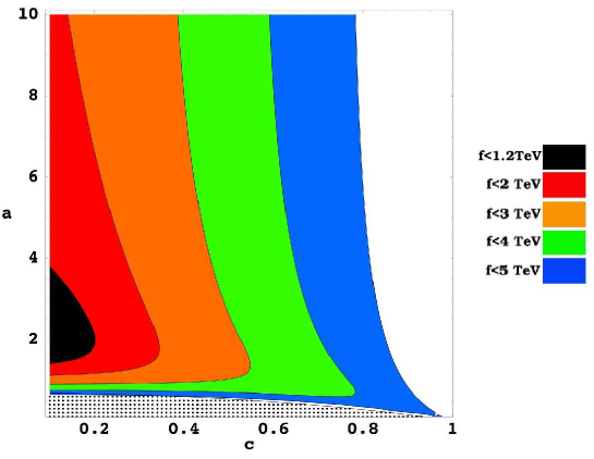
Figure 1: Contour plot of the allowed values of $f$ in the $SU(5)/SO(5)$ Littlest Higgs model with an $SU(2)\times SU(2)\times U(1)$ gauged subgroup, as a function of the parameters $c\equiv\cos\theta$ and $a$. The gray shaded region at the bottom is excluded by requiring a positive triplet mass. From Ref. [496].

The study of the LHC signatures of the Littlest Higgs model has been initiated in Refs. [498, 497, 499]; a detailed study including realistic detector simulations has been subsequently performed by the ATLAS collaboration [500]. In the preferred parameter range, the heavy $SU(2)$ gauge bosons $W_{H}^{\pm}$ and $W_{H}^{3}$ are expected to be copiously produced at the LHC by the Drell-Yan process. Their decays into lepton pairs provide a very clear signature, with the reach in this channel extending to $M(W_{H})\approx 5$ TeV for typical parameters (see Fig. 2). Other decay channels include quark pairs, which could be used to test the universality of the $W_{H}$ couplings to the fermions predicted by the model, as well as gauge boson and gauge boson-Higgs pairs, e.g. $W_{H}^{3}\rightarrow W^{+}W^{-},Zh$. The latter channels are extremely interesting because the LH model makes a clean prediction for their branching ratios,

$${\rm Br}(W_{H}^{3}\rightarrow Zh)\,=\,{\rm Br}(W_{H}^{3}\rightarrow W^{+}W^{-})\,=\,\frac{\cot^{2}2\psi}{2\cot\psi}\,{\rm Br}(W_{H}^{3}\rightarrow\ell^{+}\ell^{-}).$$ (13)

This prediction is a direct consequence of the collective symmetry breaking mechanism, and can be used to probe this mechanism experimentally [499, 501]. This requires an independent measurement of the mixing angle $\psi$, which can be obtained from the $W_{H}$ production cross section if its mass is known. The prediction can also be tested with high precision at the ILC, even running below the $W_{H}$ production threshold [502].

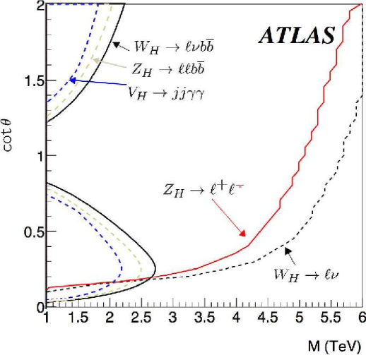
Figure 2: Accessible regions, in the $M(W_{H})-\cot\psi$ plane, for $5\sigma$ discovery at the LHC with 300 fb^-1 integrated luminosity. From Ref. [500].

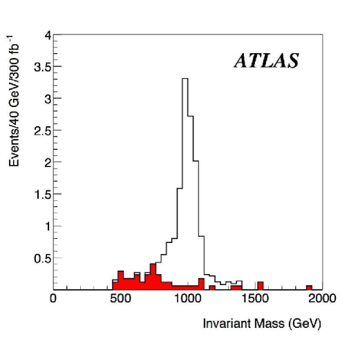
Figure 3: Invariant mass of the $Zt$ pair, reconstructed from the $\ell^{+}\ell^{-}\ell^{\pm}\nu b$ final state. The signal (white) is $T\rightarrow Zt$, computed for $M_{T}=1$ TeV, $\tan\alpha=1$, and Br$(T\rightarrow Zt)=25$%. The background (red) is dominated by $tbZ$. From Ref. [500].

The $T$ quark can be pair-produced via $q\bar{q},gg\rightarrow T\bar{T}$, or singly produced via $Wb\rightarrow T$. For most of the relevant parameter range, energy is at a premium and the single production dominates. The decays of the $T$ can be understood using the Goldstone boson equivalence theorem: in the $M_{T}\gg v$ limit, it is easy to show that

$$\Gamma(T\rightarrow th)=\Gamma(T\rightarrow tZ^{0})=\frac{1}{2}\Gamma(T\rightarrow bW^{+})\,=\,\frac{\lambda_{T}^{2}M_{T}}{64\pi}\,,$$ (14)

where $\lambda_{T}=\lambda_{t}\tan\alpha$. Additional decay modes, involving the TeV-scale gauge bosons of the Littlest Higgs model, may be kinematically allowed and contribute to the total $T$ width: for example, if the $B_{H}$ boson is present and light, the decay $T\rightarrow tB_{H}$ may be possible. All three SM decay modes in Eq. (14)provide characteristic signatures for the discovery of the $T$ at the LHC. A detailed study of the LHC discovery potential in each decay mode has been preformed by the ATLAS collaboration [500]. The $Wb$ signal, reconstructed via the $\ell\nu b$ final state, was found to be the most promising, with the $5\sigma$ discovery reach of 2000 (2500) GeV for $\tan\alpha=1$ (2) and 300 fb^-1 integrated luminosity. The $Zt$ channel, reconstructed using leptonic $Z$ decays and $t\rightarrow Wb\rightarrow\ell\nu b$, provides a clean signature with small backgrounds, as shown in Fig. 3. However, the discovery reach is somewhat below that for the $Wb$ mode due to smaller statistics: 1050 (1400) GeV with $\tan\alpha=1$ (2) and 300 fb^-1. The $ht$ mode is more challenging, but if the $T$ quark is observed in other channels and its mass is known, the $ht$ signal can be separated from background and used to check the decay pattern in Eq. (14). The cancellation of one-loop divergences in the LH model hinges on the relation

$$\frac{m_{T}}{f}=\frac{\lambda_{t}^{2}+\lambda_{T}^{2}}{\lambda_{T}}\ .$$ (15)

Once the $T$ quark is discovered, a measurement of its mass and production cross section, together with the determination of $f$ from the study of the $W_{H}$ bosons, can be used to test the relation [497].

4 LITTLEST HIGGS WITH T PARITY

While reducing the gauge group provides one possible solution to the difficulty experienced by the Littlest Higgs model in fitting the electroweak data, a more elegant solution has been proposed by Cheng and Low [503, 504]. They enlarge the symmetry structure of the models by introducing an additional discrete symmetry, dubbed “T parity” in analogy to R parity in the minimal supersymmetric standard model (MSSM). T parity can be implemented in any LH models based on a product gauge group, including the Littlest Higgs [505]. The parity explicitly forbids any tree-level contribution from the heavy gauge bosons to the observables involving only SM particles as external states. It also forbids the interactions that induce the triplet vev. As a result, corrections to precision electroweak observables are generated exclusively at loop level, the constraints are generically much weaker than in the tree-level case [506], and values of $f$ as low as 500 GeV are allowed, as illustrated in Fig. 4. The main disadvantage of these models, compared to the original Littlest Higgs, is the larger number of new particles at the TeV scale: consistent implementation of T parity requires the presence of a T-odd Dirac fermion partner for each SM weak doublet fermion. These particles are expected to be within the reach of the LHC: constraints from four-fermion operators place an upper bound on their mass, $M(f_{-})$, in units of TeV:

$$M_{\rm TeV}(f_{-})<4.8f^{2}_{\rm TeV}\,,$$ (16)

where a flavor-diagonal and universal T-odd mass has been assumed [506].

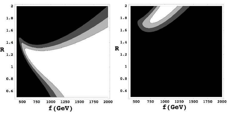
Figure 4: Exclusion contours in terms of the parameter $R\equiv\tan\alpha$ and the symmetry breaking scale $f$, in the Littlest Higgs model with T parity. In the left panel, the contribution of the T-odd fermions is neglected; in the right panel, this contribution is included assuming that it has the maximal size consistent with the constraint from four-fermion interactions, Eq. (16). From Ref. [506].

Collider phenomenology of the Littlest Higgs model with T parity was considered in Ref. [507]. While the gauge boson spectrum is similar to the original Littlest Higgs, the phenomenology is drastically different due to the fact that the TeV-scale gauge bosons are T-odd. Since all SM particles are T-even, the heavy gauge bosons must be pair-produced. The $B_{H}$ gauge boson, whose presence is obligatory in this model, is quite light, $M(B_{H})=g^{\prime}f/\sqrt{5}\approx 0.16f$, and is typically the lightest T-odd particle (LTP). Conserved T parity renders the LTP stable, and events with $W_{H}$ or $B_{H}$ production will be characterized by large missing energy or transverse momentum carried away by the two LTPs. In this sense, the signatures are very similar to SUSY models with conserved R parity or UED models with conserved Kaluza-Klein parity, raising an interesting question of how these models can be distinguished experimentally at the LHC and the ILC. One potential discriminator in the model considered in [506, 507] is the heavy top $T_{+}$, which is T-even and can be produced singly and decay via the channels listed in Eq. (14); however, T parity models with no TeV-scale T-even particles have also been constructed [508].

In analogy to SUSY neutralino, the stable LTP can play the role of a weak scale dark matter candidate, providing additional motivation for the models with T parity [507, 509].

5 OTHER LITTLE HIGGS MODELS

Starting with the “moose” model of Ref. [458], many models of EWSB incorporating the collective symmetry breaking mechanism have been constructed. These can be divided into two classes: the “product-group” models, including the Littlest Higgs along with the models in Refs. [510, 511, 512, 513], and the “simple-group” models of Refs. [514, 515, 516]. The salient phenomenological features of models within the same class are expected to be similar [501]. The simplest simple-group model, the $SU(3)$ model of [514], embeds the Higgs into an $[SU(3)/SU(2)]^{2}$ non-linear sigma model, with an $SU(3)\times U(1)$ gauged subgroup broken down to the SM $SU(2)\times U(1)$ at low energies. At the TeV scale, the model contains a set of five gauge bosons, $X^{\pm}$, $Y^{0}_{1,2}$, and $Z^{\prime}$, as well as a large number of new fermions, since all SM doublets need to be extended to complete representations of the $SU(3)$ group. Precision electroweak constraints on this model and its $[SU(4)/SU(3)]^{4}$ extension have been considered in Refs. [496, 515]. The LHC phenomenology of the $SU(3)$ model has been studied in Ref. [501], which also outlined the measurements which would need to be performed to discriminate between the product-group and simple-group models.

The non-linear sigma models of the LH theories break down at the 10 TeV scale, and need to be supplemented by a more fundamental description. Such description can involve new strongly coupled physics [517, 518], but may also be weakly coupled [519]. However, it is unlikely that the LHC experiments will be able to discern the physics beyond the nl$\sigma$m.

6 CONCLUSIONS

In this chapter, we have briefly reviewed the Little Higgs models, which provide an attractive scenario combining dynamical stabilization of the weak-Planck hierarchy by dimensional transmutation with the radiative EWSB. We concentrated on the Littlest Higgs model, two versions of which (a model with a single gauged $U(1)$ factor and a T-parity symmetric model) provide acceptable fits to precision electroweak data without significant fine tuning. The models make interesting predictions which can be tested at the LHC. More work is required in order to ensure that the LHC experiments maximize their potential in searching for the predicted signatures; to this end, it would be useful to systematically incorporate the LH model into the standard Monte Carlo packages such as PYTHIA and HERWIG.

Due to length limitations, many aspects of Little Higgs model-building and phenomenology could not be covered in this section; for more information and a comprehensive collection of references, we refer the interested reader to the recent review articles [520, 521].

Acknowledgements

This research is supported by the NSF grant PHY-0355005.

Part 28 Testing the Littlest Higgs model in $\Phi^{++}$ pair production at LHC

A. Hektor, M. Kadastik, K. Kannike, M. Müntel and M. Raidal

1 INTRODUCTION

The main motivation of the Large Hadron Collider (LHC) experiments is to reveal the secrets of electroweak symmetry breaking. If the standard model (SM) Higgs boson will be discovered, the question arises what stabilizes its mass against the Planck scale quadratically divergent radiative corrections. The canonical answer to this question is supersymmetry which implies very rich phenomenology of predicted sparticles in the future collider experiments.

More recently another possibility of formulating the physics of electroweak symmetry breaking, called the little Higgs, was proposed [488, 522, 458]. In those models the SM Higgs boson is a pseudo Goldstone mode of a broken global symmetry and remains light, much lighter than the other new modes of the model which have masses of order the symmetry breaking scale ${\cal O}(1)$ TeV. In order to cancel one-loop quadratic divergences to the SM Higgs mass a new set of heavy gauge bosons $W^{\prime},\,Z^{\prime}$ with the SM quantum numbers identical to $W\,Z,$ and a vectorlike heavy quark pair $T,\,\bar{T}$ with charge 2/3 must be introduced. Notice that those fields are put in by hand in order to construct a model with the required properties. However, the minimal model based on the $SU(5)/SO(5)$ global symmetry, the so-called littlest Higgs model [459], has a firm prediction from the symmetry breaking pattern alone: the existence of another ${\cal O}(1)$ TeV pseudo Goldstone boson $\Phi$ with the $SU(2)_{L}\times U(1)_{Y}$ quantum numbers $\Phi\sim(3,2).$

Interestingly, the existence of triplet Higgs $\Phi$ might also be required to generate Majorana masses to the left-handed neutrinos [523]. Non-zero neutrino masses and mixing is presently the only experimentally verified signal of new physics beyond the SM. In the triplet neutrino mass mechanism [524], which we assume in this work, the neutrino mass matrix is generated via

$$(m_{\nu})_{ij}=(Y_{\Phi})_{ij}v_{\Phi},$$ (1)

where $(Y_{\Phi})_{ij}$ are the Majorana Yukawa couplings of the triplet to the lepton generations $i,j=e,\mu,\tau$ which are described by the Lagrangian

$$L=i\bar{\ell}^{c}_{Li}\tau_{2}Y_{\Phi}^{ij}(\tau\cdot\Phi)\ell_{Lj}+h.c.,$$ (2)

and $v_{\Phi}$ is the effective vacuum expectation value of the neutral component of the triplet induced via the explicit coupling of $\Phi$ to the SM Higgs doublet $H$ as $\mu\Phi^{0}H^{0}H^{0}$. Here $\mu$ has a dimension of mass. In the concept of seesaw $\mu\sim M_{\Phi},$ and the smallness of neutrino masses is attributed to the very high scale of triplet mass $M_{\Phi}$ via the smallness of $v_{\Phi}=\mu v^{2}/M_{\Phi}^{2},$ where $v=174$ GeV. However, in the littlest Higgs model the triplet mass scale is ${\cal O}(1)$ TeV which alone cannot suppress $v_{\Phi}.$ Therefore in this model $\mu\ll M_{\Phi}$, which can be achieved, for example, via shining as shown in ref. [525, 526]. In that case $v_{\Phi}\sim{\cal O}(0.1)$ eV. We remind also that $v_{\Phi}$ contributes to the SM oblique corrections, and the precision data fit $\hat{T}<2\cdot 10^{-4}$ [494] sets an upper bound $v_{\Phi}\leq 1.2$ GeV on that parameter.

The cross section of the single $\Phi^{++}$ production via the $WW$ fusion process [527] $qq\to q^{\prime}q^{\prime}\Phi^{++}$ scales as $\sim v_{\Phi}^{2}.$ In the context of the littlest Higgs model this process, followed by the decays $\Phi^{++}\to W^{+}W^{+},$ was studied in ref. [498, 501, 500]. The detailed ATLAS simulation of this channel shows [500] that in order to observe $1$ TeV $\Phi^{++},$ one must have $v_{\Phi}>29$ GeV. This is in conflict with the precision physics bound $v_{\Phi}\leq 1.2$ GeV as well as with the neutrino data. Therefore the $WW$ fusion channel is not experimentally promising for the discovery of the doubly charged Higgs.

In this work we perform a Monte Carlo analyses of the Drell-Yan pair production [528, 527] $pp\to\Phi^{++}\Phi^{--}$ of the doubly charged Higgs boson followed by the leptonic decays $\Phi^{\pm\pm}\to 2\ell^{\pm}$ in a typical LHC experiment. We assume that neutrino masses come from the coupling to the triplet Higgs which fixes the $\Phi^{++}$ leptonic branching ratios. Due to the smallness of $v_{\Phi}$ we can neglect the decays to $WW.$ The advantages of this process are the following.

1. The production cross section is known, it does not depend on the unknown model parameters.

2. The decay $\Phi^{++}\to\ell^{+}\ell^{+}$ is lepton number violating and allows to reconstruct $\Phi^{++}$ invariant mass from the same charged leptons rendering the SM background very small in the signal region.

3. The known neutrino mixing Eq.(1) predicts the branching ratios as $BR(\Phi^{++}\to\mu^{+}\mu^{+})=BR(\Phi^{++}\to\tau^{+}\tau^{+})=BR(\Phi^{++}\to\mu^{+}\tau^{+})=1/3.$ We assume that neutrinos have a normal hierarchy which implies negligible decay rates to the electron final states.

We consider only the muon final states which are the easiest to observe at the LHC environment. We have generated the production process and the leptonic decays of $\Phi^{\pm\pm}$ as well as the relevant background processes using PYTHIA Monte Carlo generator [17], and analyzed both the $2\mu^{+}2\mu^{-}$ and $2\mu^{\pm}$ final states. We have used the default set of PYTHIA parameters (parton structure functions, gauge couplings etc.) except that we fix the $\Phi^{++}$ branching ratios via $Y_{\Phi}^{\mu\mu}=\sqrt{2}Y_{\Phi}^{\mu\tau}=Y_{\Phi}^{\tau\tau}=1.$ Rescaling of those couplings to satisfy data from the searches for lepton flavour violating processes [527, 529] does not affect our results. We also comment on the results of our analyses if this assumption is relaxed and $BR(\Phi^{++}\to\mu^{+}\mu^{+})=1.$

2 FOUR MUON FINAL STATES

$$\begin{array}[]{|c|c|c|c|c|}\hline\cr\hline\cr\mbox{Process}&\mbox{N of expected}&S1&S2&S3\\ &\mbox{events }&p_{T}>75\;(50)\mbox{ GeV}&\eta<2.5&2\mu^{+}2\mu^{-}\\ \hline\cr\mbox{background}&&&&\\ ZZ\to 2\mu^{+}2\mu^{-}&177&12\;(42)&9.5\;(30)&0.7\;(3.0)\\ t\bar{t}\to 2\mu^{+}2\mu^{-}&1.3\cdot 10^{8}&1.1\cdot 10^{4}\;(6\cdot 10^{4})&1\cdot 10^{4}\;(5.8\cdot 10^{4})&0\;(4.5)\\ b\bar{b}\to 2\mu^{+}2\mu^{-}&2.8\cdot 10^{10}&1.1\cdot 10^{4}\;(1.1\cdot 10^{5})&7.1\cdot 10^{3}\;(8.5\cdot 10^{4})&0\;(0)\\ \hline\cr\mbox{signal}&&&&\\ M_{\Phi}=200\mbox{ GeV}&2\cdot 10^{4}&5849\;(9182)&5340\;(8129)&818\;(1723)\\ M_{\Phi}=500\mbox{ GeV}&512&298\;(330)&287\;(314)&81\;(97)\\ M_{\Phi}=1000\mbox{ GeV}&15&9.7\;(10.1)&9.5\;(9.8)&3.1\;(3.3)\\ \hline\cr\hline\cr\end{array}$$ (13)

Table 1: The number of expected background and signal events for the integrated luminosity $300\;fb^{-1},$ and the number of $\Phi^{\pm\pm}$ candidates from the $2\mu^{+}2\mu^{-}$ final states passing each cut. For the signal events we have taken $BR(\Phi^{++}\to\mu^{+}\mu^{+})=1/3.$

Considering the four muon final states $2\mu^{+}2\mu^{-}$ as the experimental signature for the process $pp\to\Phi^{++}\Phi^{--}$ we have reconstructed the invariant mass of two like-sign muons,

$$m^{2}_{I}=(p_{1}^{\pm}+p_{2}^{\pm})^{2},$$ (14)

with the four-momentas $p_{1,2}.$ Since the like-sign signal muons originate from the same doubly charged Higgs boson, the invariant mass peak will measure the Higgs mass, $m_{I}=M_{\Phi}.$ The four muon signature is the cleanest and the most robust one. The background arises mostly from the $Z^{0}Z^{0},$ $b\bar{b},$ and $t\bar{t}$ production and their muonic decay. Because those particles are lighter than $\Phi$ (the present bound from Tevatron is $M_{\Phi}\geq 136$ GeV [530, 531]) the background muons must be softer and should not give an invariant mass peak. To enhance the signal over background we have applied three selection rules as follows. S1: all muons with transverse momentum smaller than 75 GeV (50 GeV) are neglected. The larger (smaller) $p_{T}$ cut is appropriate for the heavier (lighter) Higgs boson. S2: only the muons with pseudorapidity $\eta<2.5$ are detectable at CMS or ATLAS and only those are selected. S3: only the events with 2 positive and 2 negative muons are selected.

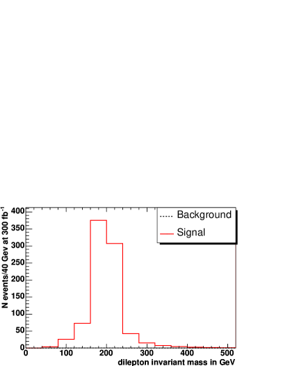
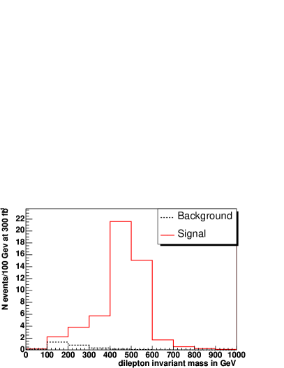
Figure 1: Distribution of the invariant mass of two like-sign muons after all cuts for the $2\mu^{+}2\mu^{-}$ final state in the case of $M_{\Phi}=200$ GeV (left panel) and $M_{\Phi}=500$ GeV (right panel) for $p_{T}>75$ GeV. The background is almost invisible.

We have generated with PYTHIA Monte Carlo the datasets of $2.8\cdot 10^{7}$ $b\bar{b},$ $t\bar{t}$ and $10^{6}$ $ZZ$ events for the background, and the datasets of $5\cdot 10^{5}$ signal events with $M_{\Phi}=200,\;500,\;1000$ GeV. We have applied the selection rules described above and rescaled the results taking into account the cross section of the particular process. In Table 1 we present the expected number of background and signal events as well as the numbers of $\Phi^{\pm\pm}$ candidates passing each selection rule. We assume the total integrated luminosity to be $300fb^{-1}$. The most effective cut is the $p_{T}$ cut and therefore applied first. As one can see, the background is almost eliminated, especially for the cut $p_{T}>75$ GeV. In Fig. 1 we plot the histogram for the invariant mass distribution of the like-sign muons passing all the cuts for $M_{\Phi}=200$ GeV and $M_{\Phi}=500$ GeV. The SM background is represented by black dashed line and the signal by red solid line. For those values of $M_{\Phi}$ the significance $S/\sqrt{B}$ is huge.

For the mass $M_{\Phi}=1$ TeV one expects only $\sim 3$ signal candidates although the total number of produced $\Phi^{\pm\pm}$ is 30. Strong signal suppression occurs is because the probability for both $\Phi^{\pm\pm}$ to decay to two muons is 1/9. The expected background is 0.7 (7.5) fake Higgs candidates depending on the $p_{T}$ cut, but the background occurs at low invariant mass. Three Poisson distributed signal events with zero background at very high invariant mass constitutes the discovery of $\Phi^{++}$ at 95% C.L. However, if $BR(\Phi^{++}\to\mu^{+}\mu^{+})=1$ we expect to get 25.9 Higgs candidates for $M_{\Phi}=1$ TeV. In this case the LHC mass reach extends up to 1.2 TeV.

3 TWO MUON FINAL STATES

$$\begin{array}[]{|c|c|c|c|c|c|c|}\hline\cr\hline\cr\mbox{Process}&\mbox{N expected}&S1&S2&S3&S4&S5\\ &\mbox{ }&2\mu^{\pm}&p_{T}^{jet}>20\mbox{ GeV}&\eta<2.5&\phi<2.5&p_{T}>50\mbox{ GeV}\\ \hline\cr\mbox{background}&&&&&&\\ b\bar{b}&2.8\cdot 10^{10}&9.4\cdot 10^{8}&2.6\cdot 10^{7}&2.5\cdot 10^{6}&1.2\cdot 10^{6}&0\\ t\bar{t}&1.3\cdot 10^{8}&1.4\cdot 10^{7}&3.6\cdot 10^{5}&1.7\cdot 10^{5}&1\cdot 10^{5}&4.4\\ WW&2.7\cdot 10^{4}&1022&885&335&204&0\\ WZ&106&111&110&62&35&1.7\\ Z\to 2\mu&1.5\cdot 10^{7}&8.6\cdot 10^{5}&6.6\cdot 10^{5}&2.6\cdot 10^{5}&1.5\cdot 10^{5}&12.8\\ Z\to 2\tau&2.5\cdot 10^{6}&1.4\cdot 10^{5}&1.1\cdot 10^{5}&4.5\cdot 10^{4}&2.6\cdot 10^{4}&0\\ ZZ&177&369&363&207&115&7.5\\ \mbox{total}&&&&&&26.4\\ \hline\cr\mbox{signal}&&&&&&\\ M_{\Phi}=200\mbox{ GeV}&2\cdot 10^{4}&1.6\cdot 10^{4}&1.6\cdot 10^{4}&1.3\cdot 10^{4}&8513&5832\\ M_{\Phi}=500\mbox{ GeV}&512&401&389&356&225&199\\ M_{\Phi}=1000\mbox{ GeV}&15&11&11&10&6&5.7\\ \hline\cr\hline\cr\end{array}$$ (30)

Table 2: The number of expected background and signal events for the integrated luminosity $300\;fb^{-1},$ and the number of $\Phi^{\pm\pm}$ candidates from the $2\mu^{\pm}$ final states passing each cut. For the signal events we have taken $BR(\Phi^{++}\to\mu^{+}\mu^{+})=1/3.$

In order to increase the LHC mass reach for $\Phi^{\pm\pm}$ discovery we also study the two like-sign muon final states. Although in this case one can identify more signal event candidates, also the background is larger. The dominant background processes giving $2\mu^{\pm}$ final states are listed in Table 2. Because the Monte Carlo generated data sets contain also additional muons from secondary processes we must also include the processes like $Z^{0}\to\mu^{+}\mu^{-}$ to the background. Combining one of the $Z$ decay products with the secondary muon we get the fake signal which has to be eliminated. The $t\bar{t},$ $b\bar{b},$ $ZZ$ background and the signal datasets are the same as in the $4\mu$ study, in addition we have generated new background datasets of $10^{6}$ events.

To minimize the background we use the following selection rules. S1: event is counted only if it contains at least one like-sign muon pair. S2: event is rejected if it contains a quark with $p_{T}^{jet}>20$ GeV. This corresponds to the jet veto and reduces the background from hadronic processes. S3: only muons with the pseudorapidity $\eta<2.5$ are observable in CMS or ATLAS experiments. S4: we require an opening angle between the two like-sign muons to be $\phi<2.5.$ S5: only muons with $p_{T}>50$ GeV are taken and the events with at least one like-sign muon pair are selected. The number of events passing each selection rule are given in Table 2. The total number of estimated background is 26 events which is larger than in the four muon case. But also the signal is more prominent.

To see the invariant mass distribution of the like-sign muons we plot in Fig. 2 the histograms for the signal (red solid) and background (dashed black) for $M_{\Phi}=500$ GeV (left panel) and $M_{\Phi}=1000$ GeV (right panel). As one can see, the invariant mass of background muons is smaller than the one of signal. Taking only the events with invariant mass $m_{I}>300$ GeV one can get background free experimental signal of $\Phi^{++}$. In this channel the doubly charged Higgs with the mass $M_{\Phi}=1050$ GeV can be discovered. Again, if $BR(\Phi^{++}\to\mu^{+}\mu^{+})=1$ we expect to get 15.9 Higgs candidates instead of 5.7, and LHC can reach 1.1 TeV $\Phi^{++}$.

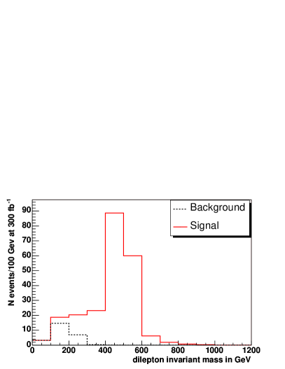
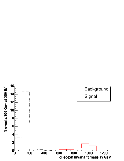
Figure 2: Distribution of the invariant mass of two like-sign muons passing all the cuts for the $2\mu^{\pm}$ final state in the case of $M_{\Phi}=500$ GeV (left panel) and $M_{\Phi}=1000$ GeV (right panel).

4 CONCLUSIONS

We have carried out Monte Carlo study of doubly charged Higgs pair production followed by the leptonic decays at the LHC experiments. Since the single $\Phi^{++}$ production is strongly suppressed, this is the only potentially observable channel at LHC. In addition, we have assumed that triplet Higgs also generates the observed neutrino masses which fixes the $\Phi^{++}$ leptonic decay branching ratios from neutrino data. We have generated the signal as well as the background processes for both four muon and two muon final states with PYTHIA Monte Carlo, and analyzed how to reduce maximally the SM background. Our results are plotted in Fig. 1 and Fig. 2 which show that the invariant mass distribution of the like-sign muon pairs allows to discover the doubly charged Higgs with the mass $M_{\Phi}=1050$ GeV. Relaxing our assumption about branching ratios, and assuming $BR(\Phi^{++}\to\mu^{+}\mu^{+})=1,$ the LHC discovery reach for $\Phi^{++}$ increases to $M_{\Phi}=1.2$ TeV

Our results can be improved by including the tau-lepton reconstruction to the analyses. The background can further be reduced via vetoing the b-tagged events and by reconstructing $Z$ and $t$, and neglecting leptons from their decays. Nevertheless, since the signal is so robust and clean, our results show that this is not necessary for $M_{\Phi}<1$ TeV.

Acknowledgements

We thank S. Lehti, A. Nikitenko and A. Strumia for useful discussions and for the technical advice. This work is partially supported by ESF grant No 6140, by EC I3 contract No 026715 and by the Estonian Ministry of Education and Research. The calculations are performed in Estonian Grid [532] and Baltic Grid.

Part 29 Polarization and spin correlation effects in third family resonances

G. Azuelos, B. Brelier, D. Choudhury, P.-A. Delsart, R.M. Godbole, S.D. Rindani, R.K. Singh and K. Wagh

1 INTRODUCTION

The properties and interactions of quarks and leptons belonging to the third family are still relatively poorly measured. The question arises, therefore, if they are just a copy of those of the first two families. The universality of interactions is a natural prediction of the Standard model (SM), but the number of generations and the relative masses in the model seem completely ad hoc. Serious constraints have been set on the universality of couplings of the first two generations, but for the third, it is less well tested. There are, in fact, reasons to believe that different electroweak and/or strong couplings might apply in this case. For example, although the LEP precision measurements are generally in very good agreement with the SM, the forward-backward asymmetry at the $Z$ pole, in the $b\bar{b}$ channel is 2.8 standard deviations away from the fitted value [450].

A study of properties of the third generation of fermions is of utmost importance from a theoretical standpoint as well. The Higgs mechanism of Spontaneous Symmetry Breaking is the only aspect of the Standard Model (SM) which still lacks direct verification. The large mass of the third generation fermions and their consequent large couplings to the Higgs boson motivate a detailed study of their properties and couplings to the gauge bosons and Yukawa couplings to the Higgs bosons. As a matter of fact, such studies are a focus of all the collider-based investigations which wish to probe/establish the Higgs mechanism. Furthermore, any alternative to the Higgs mechanism almost certainly involves the top quark [533]. Many theories beyond the SM incorporate a special role for the top quark, because of its high mass, $m_{t}\sim v/\sqrt{2}$, where $v$ is the vacuum expectation value (vev) of the SM Higgs fields. The well known problem of the instability of the Higgs boson mass to radiative corrections is solved in Supersymmetry by cancellation of the divergent contribution due to particle loops by the corresponding contribution from the sparticle loops. To cancel the dominant top quark contribution, without the use of Supersymmetry, some models, such as the Little Higgs model [534, 458], predict the existence of an additional heavy isosinglet quark, a heavy top, which could then generally mix with the SM top quark. In Technicolor models, bosons from an extended gauge group can provide mass to the light fermions, but only a fraction of the top mass can thus be explained, and one must resort to a topcolor assisted Technicolor model (TC2) [535] to understand the observed high mass of the top. For these reasons, it will be important to measure with precision the coupling constants of this mysterious quark.

The large mass of the $t$ implies that its life time is shorter than the hadronization time scale and thus the decay products maintain the memory of the polarization of the parent (anti)quark. This is normally reflected in the energy and the angular distribution of the decay lepton as well as in the correlation between the two leptons [536]. Similarly the polarization of the $\tau$ lends itself to a measurement through the energy distribution of the decay pions even at a hadronic collider [537, 538, 539]. Any anomalous interactions that the third generation fermions may have, if chirality or parity violating, may give rise to net polarization of the produced fermion. In the Higgs sector, the effects are also enhanced due to the large mass of these fermions. The possibility of exploiting the polarization of the top to probe new physics at hadron colliders [540], in the continuum $t\bar{t}$ pair production [541, 542] as well as single top production [543, 544, 545] has been subject of many studies. Studies in the context of the resonant $t\bar{t}$ production such as in Higgs decay [546] or due to s-channel exchange of a spin-2 KK graviton in the Extra Dimensional Models [547] have also been performed. The use of final state particle polarization in the probe of new physics at the LHC is currently gathering momentum as many experimental strategies continue being sharpened. In this note, we explore the possibility of using the polarization of the third family fermions produced in the decay of narrow spin-1 resonances at the LHC. In general, resonances of electroweak or strong interaction nature, of different spins, are predicted in a variety of models: (i) $Z^{\prime}$ in a Left-Right symmetric model, or in E(6) Grand Unified theory [548], (ii) $Z_{H}$ in the Little Higgs model [534, 458], (iii) Kaluza-Klein states of a graviton, in models with large extra dimensions [403], (iv) Kaluza-Klein states of the $Z$ and $\gamma$ in TeV^-1-size models of extra dimensions [549] or in (v) Higgsless models [550], (vi) $\eta_{8},\pi_{T}$ in Technicolor models, in particular TC2 models [535], or (vii) axigluons in chiral colour models [551], etc. The Tevatron has looked for such resonances and an intriguing excess of events in $t\bar{t}$ invariant mass distributions is seen [552, 553]. If such a resonance is found at future colliders, a theoretical interpretation will require a measurement of all its properties. Some obvious observables are the cross section, the width, the branching ratios to the different fermions, and forward-backward asymmetries in their decays. Here, we examine the resolving power of another observable, namely the polarization of the decay products, when such a measurement is possible, i.e. from resonance decays to $\tau\bar{\tau}$ and $t\bar{t}$.

The present study is at generator level. It aims to explore the differences between theoretical models for a future more realistic experimental analysis. The differences shown here will certainly be considerably attenuated by detector resolutions and efficiencies. In the first section we present results of a study of the tau polarization and the spin correlations in the process $Z^{\prime}\to\tau\bar{\tau}$ with a $Z^{\prime}$ with different assumed couplings. We then discuss the predictions for polarization of the $t$ in the decay of the resonance, in a particular model, the Littlest Higgs model [498]. Following this, we explore possible observables one could construct in the case of the $t\bar{t}$ pair produced resonantly. More detailed studies with the variables we have constructed and the spin-spin correlations between the decay leptons as well as the $t\bar{t}$ still remain. So do the investigations into other representative models of a Vector resonance like an axigluon [551] where the production rates will be higher, still remain to be pursued.

2 SPIN CORRELATIONS IN $Z^{\prime}\to\tau\bar{\tau}$

To study tau polarization and spin correlations in the process $Z^{\prime}\to\tau\bar{\tau}$, the program Tauola [554] was modified to include a $Z^{\prime}$ resonance. The changes were very simple: it was sufficient to add the case where the parent of a $\tau$ was a $Z^{\prime}$ and clone the $Z/\gamma$ treatment for the calculation of the probability of longitudinal polarization combinations of the $\tau$ leptons, at the level of the amplitudes, thus ensuring that all interferences are taken into account.

We have evaluated the following spin sensitive observables, as suggested in [555], for the case, expected to be the most sensitive, of $\tau\to\pi\nu$ (more generally, to include leptonic decay or three-prong decays, one can replace the $\pi$ by the system of charged particles from the decay of the $\tau$):

1. the $\pi$ energy spectrum, relative to the $\tau$ energy, in the laboratory frame: $z_{\pm}=p_{\pi^{\pm}}/E_{\tau}$,

2. the distribution of number of events as a function of the $\pi^{+}\pi^{-}$ Energy-Energy correlation variable $z_{s}$. After evaluating $a=z_{+}^{\mathrm{measured}}-z_{-}^{\mathrm{measured}}$, this variable $z_{s}$ is defined as the signed part of the surface area in the 2-parameter phase space {$z_{+}$, $z_{-}$} between lines $z_{+}$ = $z_{-}$ and $z_{+}$ = $z_{-}+a$ (the sign of the $a$ should be taken).

3. the $\pi^{+}\pi^{-}$ invariant mass.

In order to evaluate the sensitivity to couplings, a vector resonance, $Z^{\prime}$, of mass 1 TeV, was considered under different coupling scenarios: (i) Standard Model-like couplings, (ii) $\sin^{2}\theta_{W}=0$ (which could find some justification [556] in the Higgsless model) and (iii) a right-handed $Z^{\prime}$, as well as (iv) a case with no $\tau$ polarization. Effects of initial or final state radiation are included, but it must be stressed that no detector effects are applied, except for a lower $p_{T}$ cut of 30 GeV and a pseudo-rapidity cut of $|\eta|<2.5$ on the emitted $\pi$’s. The distributions obtained represent, therefore, parton-level distributions, where reconstruction efficiencies or resolutions have not been taken into account. The reconstruction of a $\tau$-pair resonance is possible at the LHC, in spite of the presence of neutrinos in the final state. Neglecting the mass of the $\tau$ leptons and making the approximation that the neutrino transverse momenta are in the same direction as the $\tau$ itself: with the measurement of $p_{T}^{miss}$ and momentum vectors of the charged decay products, there are enough constraints to reconstruct fully the kinematics [557]. The method, however, has a singularity when the two $\tau$’s are exactly back to back, which occurs when the resonance is very heavy, and essentially produced at rest. It must be expected, therefore, that the sensitivities obtained above at parton level will be considerably degraded when applied at detector reconstruction level. This will be the subject of a future study.

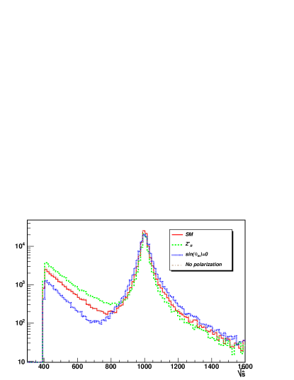
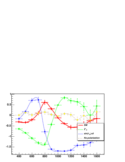
Figure 1: (a) The $Z^{\prime}$ resonance and the Drell-Yan background. Colors and line styles as shown. (b) $z_{-}$: normalized slope of the distribution of $E_{\pi^{-}}/E_{\tau^{-}}$ in the laboratory frame, as a function of the invariant mass of the two $\tau$’s.

Fig. 1$(a)$ shows the shape of the resonance in the different scenarios, together with the Drell-Yan continuum ($Z/\gamma$ s-channel contribution and interferences) whereas Fig. 1$(b)$ shows the slope of the $z_{-}$ distribution as a function of the invariant mass of the two $\tau$’s. The interference region of the Drell-Yan and $Z^{\prime}$ resonance is particularly sensitive to its couplings.

It is interesting to compare the distribution of the normalized $\pi\pi$ invariant mass in the presence of the $Z^{\prime}$ with that for the SM Drell-Yan tail, in the interference region. As can be seen the shape of the $\pi\pi$ invariant mass distribution, shown in Fig. 2 is not much altered by the presence of a $Z^{\prime}$ resonance with SM couplings, but changes very significantly for the other cases studied, with different couplings.

  

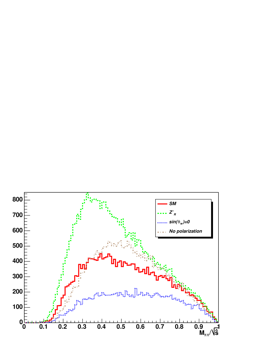
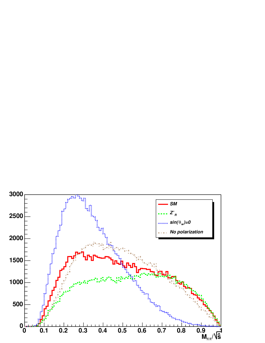
Figure 2: Invariant mass of the two pions from $\tau\bar{\tau}$ decay. Left panel: in the Drell-Yan region ($\sqrt{\hat{s}}<800$ GeV); Right panel: in the $Z^{\prime}$resonance region ($\sqrt{\hat{s}}>800$ GeV)

Fig. 3$(a)$ shows the sensitivity to the couplings of the Forward-Backward asymmetry in the decay of the $Z^{\prime}$, defined as

$$A_{FB}=\frac{N_{+}-N_{-}}{N_{+}+N_{-}}$$

where $N_{\pm}$ is the number of events where, the $\tau^{\pm}$, in the cm frame of the $Z^{\prime}$, has the same $p_{z}$ direction as that of the $Z^{\prime}$, in the laboratory frame. The $Z^{\prime}$ direction is strongly correlated with the direction of the quark, and anticorrelated with that of the antiquark, from which it was produced. The distribution of the variable $z_{s}$, shown in Fig. 3(b), is only sensitive to the vector nature of the resonance. The case with no polarization of the $\tau$’s would lead to a perfectly flat distribution if no cuts had been applied.

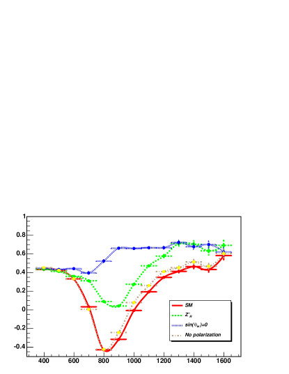
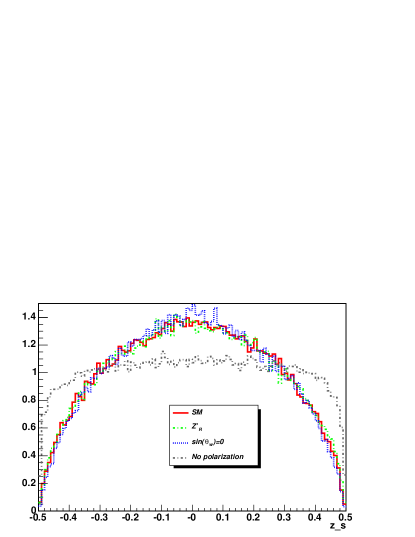
Figure 3: (a) Forward-Backward asymmetry as a function of the invariant mass of the two $\tau$’s. (b) Distribution in the $z_{s}$ variable defined in the text.

It is interesting to note that in the Littlest Higgs model [498] which we consider below for the $t\bar{t}$ case, one expects the decay $\tau$’s to be completely left handed polarized as opposed to about $40\%$ expected for a $Z^{\prime}$ with the SM couplings. So that even with a moderately good determination of the $\tau$ polarization, one can have good discriminatory power for models.

3 $t\bar{t}$ RESONANCE

Contrary to the $\tau\tau$ case above, the background for a $t\bar{t}$ resonance follows from a strong interaction process from the colliding protons ($gg\to t\bar{t}$ and $qq\to t\bar{t}$) at the LHC and can therefore dominate the signal. Nevertheless, even with a low signal/background ratio, if the mass of the resonance is known from observation in some other channel, one could be sensitive [558] to the presence of a resonance and could hope to detect a variation in the spin effects around that mass. It must be noted that the backgrounds will be much more manageable at the ILC.

3.1 EXPECTED POLARIZATION IN THE LITTLEST HIGGS MODEL

Rather than consider a generic $Z^{\prime}$, we choose to demonstrate our results for a specific choice, namely the vector resonance expected in the Littlest Higgs model [498]. For such a choice of $Z_{H}$, the fermionic couplings can be parametrized in terms of the electroweak coupling $g$ and a single mixing angle $\theta$, namely

$$(v_{f},a_{f})=\pm(g\ \cot\theta/4,-g\ \cot\theta/4)\quad\mbox{for}\ T_{3}=\pm 1/2$$ (1)

Phenomenological consistency demands that $1/10\leq\cot\theta\leq 2$. The theory has two mass scales $v$ and $f$ which respectively are the vevs of the electroweak and the heavy Higgs. The mass of the $Z_{H}$ is a linear function of the higher scale $f$ and is larger than $m_{W}(2f/v)$. In our analysis, we consider a mass range of $500\ {\rm GeV}\leq m_{Z_{H}}\leq 1500\ {\rm GeV}$. The decay width of the $Z_{H}$ is determined uniquely in terms of its mass and $\cot\theta$, and is dominated by the partial decay widths into the fermions, on account of its coupling to the SM gauge bosons being suppressed by a relative factor of $v/f\approx 1/20$ [498]. For the range of parameters that we are interested in, $\Gamma(Z_{H})\>\raisebox{-2.15277pt}{$\stackrel{{\scriptstyle\textstyle<}}{{\sim}}$}\>15\ {\rm GeV}$ with the higher values reached only for $\cot\theta\sim 2$.

With the introduction of the $Z_{H}$, the top-pair production process receives an additional $s$-channel contribution. Given that the axial coupling of the $Z_{H}$ is non-zero (Eq.1), clearly this diagram would contribute unequally to the production of $\overline{t_{L}}t_{L}$ vs. $\overline{t_{R}}t_{R}$ pairs and $\overline{t_{L}}t_{R}$ vs. $\overline{t_{R}}t_{L}$ pairs (note that the subscripts $L,R$ refer here to helicity and not chirality). It thus becomes interesting to consider the expected polarization for the $t\bar{t}$ system defined through

$$P_{t} = \frac{\sigma(t_{L})-\sigma(t_{R})}{\sigma(t_{L})+\sigma(t_{R})}$$ (2)

Clearly, the contribution of the new gauge boson would be most apparent around the $Z_{H}$ peak in the invariant-mass distribution of the top-pair. This is illustrated in Fig. 4, for both the total cross section as well as for the difference of the cross-sections for the right and left handed polarized top quarks. The latter does have a non-zero value even within the SM (on account of the contribution of the ordinary $Z$), but is magnified by a few orders close to the $Z_{H}$ peak. Understandably, this magnification is far less muted for the total cross section as the latter, within the SM, is dominated by the strong interaction contribution.

Figure 4: $d\sigma/dq$ as a function of the invariant mass $q$ of the $t\bar{t}$ system. The upper (lower) panel shows the sum (difference) of the cross-sections for the right and left handed polarized top, for $M_{Z^{\prime}}$=1000 GeV and $\cot{\theta}$=2.0. We have used the MRST(LO) 2001 parametrisation of the parton densities [559]and have used the $Q^{2}=q^{2}$.

To enhance the sensitivity, we concentrate on a $t\bar{t}$ sample centred around the resonance, restricting ourselves to $|m_{t\bar{t}}-m_{Z_{H}}|\leq dm$, where $dm=\max(10,3\Gamma_{Z_{H}})$. On imposition of this condition, we find that the polarization given by Eq. 2 can be as large as 24% while the SM prediction for the same is of the order $10^{-2}\%$. The contours of the expected polarization $P_{t}$ are shown in Fig. 5$(a)$.

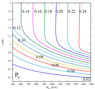
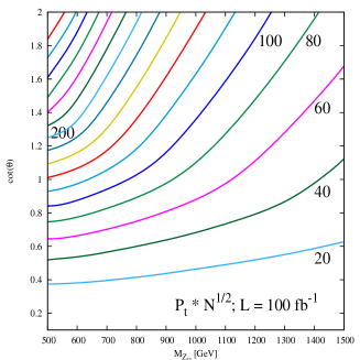
Figure 5: (a) Contours of expected polarization for the $\bar{t}t$ pair (See Eq.2) in the $m_{Z_{H}}$–$\cot\theta$ plane. (b) Contours of statistical significance for the degree of polarization assuming an integrated luminosity of $100\ {\rm fb}^{-1}$.

Note that $P_{t}$ increases with the mass $m_{Z_{H}}$ for a fixed value of coupling $\cot\theta$. On the other hand, the rates decrease with the increasing invariant mass $m_{t\bar{t}}$, thereby pulling down the sensitivity. A measure of the statistical significance is given by the ratio $P_{t}/\delta P_{t}$, and in Fig. 5$(b)$, we show the contours for the same for an integrated luminosity of 100 fb^-1. It should be noted that we have used the rates for the $t\bar{t}$ production for estimating the sensitivity and in any realistic measurement the sensitivity is expected to go down. For example, the asymmetries constructed in terms of angular distributions/correlations of the decay leptons from top-quarks will suffer a reduction in statistics due to the branching ratios and realistic angular cuts will further reduce the useful number of events. Note also that one might gain by a factor of $\sqrt{2}$ in the senstivity by considering either of the $t\,(\bar{t})$ to decay. Even if the abovementioned reduction factor is as large as 10, one may still have sensitivity to a heavy neutral gauge boson $Z_{H}$ over large part of the parameter space shown in Fig. 5$(b)$. We note that the resonance signal may be difficult to see at the LHC (an example of $Z_{H}\to t\bar{t}$ reconstruction at the LHC can be found in [560]), but the polarization effects may nevertheless be measurable.

3.2 TOP POLARIMETRY

Our main objective is to explore experimentally viable variables sensitive to the top quark polarization. Clearly, if such variables can be constructed out of lepton distributions alone, they would be more robust in the context of the LHC. To begin with, we consider distributions of lepton observables in the laboratory frame since these are most easily measured experimentally. They will, however, be sensitive to the rapidity distribution of the $Z^{\prime}$. The analysis of distributions in the center of mass frame of the hard scattering will be the subject of a further study. The energy distribution of the leptons in the laboratory frame is shown in Fig. 6. Although the normalized distributions do show a difference between the two cases of a net left polarization for the top and that with a net right polarization, it is difficult to construct a suitable variable that would be relatively free of normalization uncertainties of the cross-section predictions.

Since the sensitivity of the lepton energy distribution to $P_{t}$ is low, we next consider their angular distributions for, as has been shown in Refs.[561, 562, 563], these are independent of any anomalous contributions from top decay ($tbW$) vertex. Thus, these could constitute potent and robust probes of the parent top polarization. An obvious candidate is the forward backward asymmetry in the distribution of leptons, with the polar angle being measured with respect to the boost direction of the $t\bar{t}$ center of mass frame. However, this variable turns out to be only very mildly sensitive to the magnitude of top quark polarization but almost insensitive to the sign of polarization. This, in a large part, is due to the cancellation of the effect between the products of diagonal and off diagonal terms of production and decay density matrices. Similar is the case for the distribution in the angle between top quark and lepton in the laboratory. While this variable has sensitivity to both the sign and magnitude of the top quark polarization, it involves the detailed construction of the top momentum and the consequent sensitivity is marginal.

      

Figure 6: Normalized lepton distributions for a $Z^{\prime}$ mass of 500 GeV and different couplings of the $Z^{\prime}$. Also shown are the corresponding curves for the SM. (a) the energy $E_{l}$ and (b) the azimuthal angle $\phi_{l}$.

Finally, we consider the azimuthal angle of the decay lepton, $\phi_{l}$, measured with respect to the plane defined by the top-quark direction and the axis along which the protons collide. Note that the direction of the momentum of the parton center-of-mass frame is irrelevant. It can be shown that the dependence on $\phi_{l}$ comes only through $\cos(\phi_{l})$ and hence will be symmetric under a change $\phi_{l}$ to $2\pi-\phi_{l}$. The $\phi_{l}$ dependence is controlled by the spins of the particles and the boosts involved. The distribution is peaked near $\phi_{l}=0,\pi$ due to the kinematic effect of the boost in going from the $t$ rest frame to the laboratory frame. The height of this peak is sensitive to the $t$ polarization. Thus the distribution in $\phi_{l}$ could provide a probe of $t$ polarization. The distribution presented in Fig. 6$(b)$ shows that it is sensitive not only to the magnitude but also to the sign of top-quark polarization. This prompts us to construct an asymmetry by contrasting events with a lepton in either of $1^{st}$ & $4^{th}$ quadrants (i.e. $0\leq\phi_{l}<\frac{\pi}{2}$ or $\frac{3\pi}{2}\leq\phi_{l}<2\pi$) with those with a lepton in either of $2^{nd}$ & $3^{rd}$ quadrants (i.e. $\frac{\pi}{2}\leq\phi_{l}<\frac{3\pi}{2}$), or in other words,

$$A \equiv \frac{\sigma(1,4)-\sigma(2,3)}{\sigma(1,4)+\sigma(2,3)}$$ (3)

For ease of analysis, it is useful to construct an observable $O$ of the form

$$O = A_{Z^{\prime}}-A_{SM}$$ (4)

with the consequent sensitivity $S$ to the observable $O$ being given by

$$S = O\left(\frac{\sigma_{Z^{\prime}}*L}{1-A_{SM}^{2}}\right)^{\frac{1}{2}}$$ (5)

In other words, $S$ is just the significance level of $O$ being different from zero. We calculate $O$ and $S$ over the allowed region of $\cot{\theta}$ and $M_{Z^{\prime}}$ values for the Littlest Higgs Model. The results displayed in Figs. 7 for $M_{Z^{\prime}}$ ¡ $1000\>\rm GeV$ show that $O$ reflects well the degree of polarization of the top-quark That they are not exactly the same is but a consequence of kinematical effects as mentioned in the captions of Figs. 7.

   

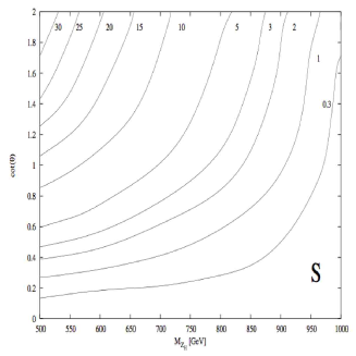
Figure 7: (a) The observable $O$ as a function of $\cot{\theta}$ and $M_{Z^{\prime}}$. As can be seen from Fig. 5, for constant $M_{Z^{\prime}}$ the observable follows the same trends as the top-quark polarization. However, there are some kinematical effects which lead to different trends for constant couplings and varying $M_{Z^{\prime}}$, as compared to top-quark polarization. (b) The sensitivity $S$ for the observable $O$ as a function of $\cot{\theta}$ and $M_{Z^{\prime}}$. As can be seen from Fig. 5($b)$, $S$ follows the same trends as top-quark polarization sensitivity.

3.3 SPIN SPIN CORRELATIONS

As mentioned already, the spin-spin correlations between the $t$ and $\bar{t}$ and the consequent correlations between the decay leptons will also carry this spin information. Top polarization in the continuum $t\bar{t}$ process from $gg$ or $qq$ fusion has been implemented in the generators Toprex [564] and AcerMc [564]. Production via a scalar resonance (Higgs) has also been implemented. As mentioned earlier, studies also exist for the effect of a Spin 2, KK graviton. We quote here one of the observables of top spin correlations, following [565], where, for simplicity, we assume a decay $t\bar{t}\to W^{+}bW^{-}\bar{b}\to e^{+}\nu bq\bar{q}^{\prime}b$:

1. the correlation in angular distribution of the two top quarks:

   $$\frac{1}{N}\frac{d^{2}N}{d\cos\theta_{1}\leavevmode\nobreak\ d\cos\theta_{2}}=\frac{1}{4}(1+B_{1}\cos\theta_{1}+B_{2}\cos\theta_{2}-C\cos\theta_{1}\cos\theta_{2})$$ (6)

   where $\theta_{1}$ ($\theta_{2}$) are respectively the angles between the direction of the $e^{+}$ ($e^{-}$) in the rest frames of $t$ ($\bar{t}$,) and the direction of the $t$ ($\bar{t}$) in the rest frame of the $t\bar{t}$ system.

2. the distribution of the opening angle $\Phi$ between the two leptons

   $$\frac{1}{N}\frac{dN}{d\cos\Phi}=\frac{1}{2}(1-D\cos\Phi)$$ (7)

Such studies applied to a $Z^{\prime}$ with arbitrary couplings still need to be implemented.

4 CONCLUSIONS

Resonances involving third generation fermions can reveal valuable information on effects beyond the Standard Model. Here, studies of polarization and spin correlation observables for heavy $\tau\bar{\tau}$ and $t\bar{t}$ resonances at the LHC have been performed at parton level and other observables have yet to be evaluated. These initial studies show that there is some sensitivity to the couplings of such resonances. More work needs to be done, however, to evaluate in more realistic scenarios, involving detector simulation and reconstruction effects, the possibility of using these observables in determining the couplings of these resonances to the $\tau$ leptons and $t$ quarks.

Acknowledgements

We thank Z. Was for helpful discussions. RG, SDR and RKS wish to acknowledge partial support from the IndoFrench Centre for Cooperation in Advanced Research (IFCPAR) under project number IFC/3004-B/2004.

Part 30 Charged Higgs boson studies at the Tevatron and LHC

V. Bunichev, L. Dudko, S. Hesselbach, S. Moretti, S. Perries, J. Petzoldt, A. Pompoš, J. Rathsman and A. Sopczak

1 INTRODUCTION

The importance of charged Higgs boson searches at future colliders has in the recent years been emphasized [566, 567, 568, 177] for LEP, a future International Linear Collider (ILC), the Tevatron and the Large Hadron Collider (LHC), as the detection of the charged Higgs boson would be a definite signal for the existence of New Physics going beyond the Standard Model (SM) [569, 570]. The charged Higgs boson states are naturally accommodated in non-minimal Higgs scenarios, like the Two-Higgs Doublet Models (2HDMs). A Supersymmetric version of the latter is the Minimal Supersymmetric Standard Model (MSSM). It is a Type II 2HDM with specific relations among neutral and charged Higgs boson masses and couplings, dictated by Supersymmetry (SUSY) [571].

The Tevatron collider at Fermilab is currently in its second stage of operation, so-called Run 2, with a higher center-of-mass (CM) energy of $\sqrt{s}=1.96$ TeV. This machine will be the first one to probe charged Higgs boson masses in the mass range up to $m_{H^{\pm}}\sim m_{t}$ [568]. Starting from 2008, the LHC at CERN will be in a position to confirm or rule out the existence of such a particle over a very large portion of both the 2HDM and MSSM parameter space, $m_{H^{\pm}}\lower 3.01385pt\hbox{$\;\stackrel{{\scriptstyle\textstyle<}}{{\sim}}\;$}400$ GeV, depending on $\tan\beta$ (see the reviews [572, 573, 574]).

At present, a lower bound on the charged Higgs boson mass exists from LEP [575], $m_{H^{\pm}}\lower 3.01385pt\hbox{$\;\stackrel{{\scriptstyle\textstyle<}}{{\sim}}\;$}m_{W}$, independently of the charged Higgs boson decay Branching Ratios (BRs). This limit is valid within any Type II 2HDM whereas, in the low $\tan\beta$ region (below about 3), an indirect lower limit on $m_{H^{\pm}}$ can be derived in the MSSM from the one on $m_{A}$ (the mass of the pseudoscalar Higgs state of the model): $m_{H^{\pm}}^{2}\approx m_{W}^{2}+m_{A}^{2}\lower 3.01385pt\hbox{$\;\stackrel{{\scriptstyle\textstyle>}}{{\sim}}\;$}(130\leavevmode\nobreak\ \mathrm{GeV})^{2}$.

If the charged Higgs boson mass $m_{H^{\pm}}$ satisfies $m_{H^{\pm}}<m_{t}-m_{b}$, where $m_{t}$ is the top quark mass and $m_{b}$ the bottom quark mass, $H^{\pm}$ particles could be produced in the decay of on-shell (i.e., $\Gamma_{t}\to 0$) top (anti-)quarks $t\rightarrow bH^{+}$, the latter being in turn produced in pairs via $gg$ fusion and $q\bar{q}$ annihilation. This approximation was the one customarily used in event generators when $m_{H^{\pm}}\lower 3.01385pt\hbox{$\;\stackrel{{\scriptstyle\textstyle<}}{{\sim}}\;$}m_{t}$. Throughout this paper we adopt the same notation as in Ref. [576]: charged Higgs production is denoted by $q\bar{q}$, $gg\rightarrow t\bar{t}\rightarrow tbH^{\pm}$ if due to (anti-)top decays and by $q\bar{q}$, $gg\rightarrow tbH^{\pm}$ if further production diagrams are included. Owing to the large top decay width ($\Gamma_{t}\simeq 1.5$ GeV) and due to the additional diagrams which do not proceed via direct $t\bar{t}$ production [577, 578, 579], charged Higgs bosons could also be produced at and beyond the kinematic top decay threshold. The importance of these effects in the so-called ‘threshold’ or ‘transition’ region ($m_{H^{\pm}}\approx m_{t}$) was emphasized in previous Les Houches proceedings [580, 581] as well as in Refs. [576, 582, 583, 584] and the calculations of Refs. [577, 578] (based on the appropriate $q\bar{q},gg\to tbH^{\pm}$ description) are now implemented in HERWIG [585, 11, 13, 12] and PYTHIA [586, 17, 16, 46, 587]. (A comparison between the two generators was carried out in Ref. [576].) For any realistic simulation of $H^{\pm}$ production with $m_{H^{\pm}}\lower 3.01385pt\hbox{$\;\stackrel{{\scriptstyle\textstyle>}}{{\sim}}\;$}m_{t}$ the use of these implementations is of paramount importance. In addition, in the mass region near the top quark mass, a matching of the calculations for the $q\bar{q},\leavevmode\nobreak\ gg\rightarrow tbH^{\pm}$ and $gb\rightarrow tH^{\pm}$ processes might be required [587].

A charged Higgs boson with $m_{H^{\pm}}\lower 3.01385pt\hbox{$\;\stackrel{{\scriptstyle\textstyle<}}{{\sim}}\;$}m_{t}$ decays predominantly into a $\tau$ lepton and a neutrino. For large values of $\tan\beta$ ($\;\stackrel{{\scriptstyle\textstyle>}}{{\sim}}\;$ 5), the ratio of the vacuum expectation values of the two Higgs doublets, the corresponding branching ratio is near 100%. For $m_{H^{\pm}}\lower 3.01385pt\hbox{$\;\stackrel{{\scriptstyle\textstyle>}}{{\sim}}\;$}m_{t}$, $H^{\pm}\to\tau\nu$ is overwhelmed by $H^{\pm}\to tb$, but the latter is much harder to disentangle from background than the former. The associated top quark decays predominantly into a $W$ boson, or at times a second charged Higgs boson, and a $b$ quark. The reaction

$$q\bar{q},gg\to tbH^{\pm}\leavevmode\nobreak\ \leavevmode\nobreak\ \leavevmode\nobreak\ (t\to bW)\leavevmode\nobreak\ \leavevmode\nobreak\ \leavevmode\nobreak\ (H^{\pm}\to\tau^{\pm}\nu_{\tau})$$ (1)

is then a promising channel to search for the charged Higgs boson at both the Tevatron (where the dominant production mode is $q\bar{q}$) and the LHC (where $gg$ is the leading subprocess). If the $H^{\pm}\to\tau\nu$ decay channel is used to search for Higgs bosons, then a key ingredient in the signal selection process should be the exploration of decay distributions that are sensitive to the spin nature of the particle yielding the $\tau$ lepton ($H^{\pm}$ or $W^{\pm}$), as advocated in Refs. [538, 588, 589, 590] (see also [591, 592]).

It is the purpose of this contribution to outline the possible improvements that can be achieved at the Tevatron and LHC in the search for charged Higgs bosons, with mass below, near or above $m_{t}$, when both the appropriate description of the Higgs production process and polarization effects are used to sharpen the $H^{\pm}\to\tau\nu$ signature.

2 EXPERIMENTAL SIMULATION AT THE TEVATRON ENERGY

We start by studying charged Higgs production $q\bar{q},gg\to tbH^{\pm}$ with subsequent decays $t\to bW$, $H^{\pm}\to\tau^{\pm}\nu_{\tau}$ at the FNAL Tevatron with $\sqrt{s}=1.96$ TeV. In the following we analyse hadronic decays of the $W$ boson and $\tau$ lepton ($W\to q\bar{q}^{\prime}$, $\tau\to\mathrm{hadrons}+\nu_{\tau}$), which results in the signature $2b+2j+\tau_{\mathrm{jet}}+\not\!P_{t}$ (2 $b$ jets, 2 light jets, 1 $\tau$ jet and missing transverse momentum). The most important background process is $q\bar{q},gg\to t\bar{t}$ with the subsequent decays $t\to bW^{+}$ and $\bar{t}\to\bar{b}W^{-}$, one $W$ boson decaying hadronically ($W\to q\bar{q}^{\prime}$) and one leptonically ($W\to\tau\nu_{\tau}$), which results in the same final state particles as for the expected signal.

The signal process $q\bar{q},gg\to tbH^{\pm}$ is simulated with PYTHIA [586, 17, 16, 46] using the implementation described in [587], in order to take the effects in the transition region into account. The subsequent decays $t\to bW$, $W\to q\bar{q}^{\prime}$ and $H^{\pm}\to\tau^{\pm}\nu_{\tau}$ are carried out within PYTHIA, whereas the tau leptons are decayed externally with the program TAUOLA [554, 593], which includes the complete spin structure of the $\tau$ decay. The background process $q\bar{q},gg\to t\bar{t}$ is also simulated with PYTHIA with the built-in subroutines for $t\bar{t}$ production. Here, the decays of the top quarks and $W$ bosons are performed within PYTHIA and that of the $\tau$ lepton within TAUOLA.

The momentum of the final $b$ and light quarks from the PYTHIA event record is taken as the momentum of the corresponding jet, whereas for the $\tau$ jet the sum of all non-leptonic final state particles as given by TAUOLA is used. The energy resolution of the detector is emulated through a Gaussian smearing $(\Delta(P_{t})/P_{t})^{2}=(0.80/\sqrt{P_{t}})^{2}$ of the transverse momentum $P_{t}$ for all jets in the final state, including the $\tau$ jet [568]. The $\tau$-spin information affects both the energy and the angular distribution of the $\tau$ decay products. As a basic cut the transverse momenta of these final jets are required to be larger than $5$ GeV. The missing transverse momentum $\not\!P_{t}$ is constructed from the transverse momenta of all visible jets (including the visible $\tau$ decay products).

The signal and background processes have been simulated for $\tan\beta=30$ and $m_{H^{\pm}}=80,100$ and $160$ GeV with PYTHIA, version 6.325. As shown in [576], the signal cross section $tbH^{\pm}$ agrees with the one from the top-decay approximation $t\bar{t}\to tbH^{\pm}$ for charged Higgs boson masses up to about 160 GeV. For this to be true the same factorization and renormalization scales have to be used, as well as the same scale for the running $b$ quark mass. In this study we have used the factorization scale $(m_{t}+m_{H^{\pm}})/4$ [587], the renormalization scale $m_{H^{\pm}}$, and the running $b$ quark mass has been evaluated at $m_{H^{\pm}}$ for both the signal and the background for consistency. This results in a dependence of the background calculations on $\tan\beta$ and $m_{H^{\pm}}$. However, the cross sections have then been rescaled with a common factor such that the total $t\bar{t}$ cross section is $\sigma^{\rm prod}_{t\bar{t}}=5220$ fb [594]. The resulting cross sections into the final state with the signature $2b+2j+\tau_{\mathrm{jet}}+\not\!P_{t}$ for signal and background are given in Table 1 before ($\sigma^{\rm th}$) and after ($\sigma$) applying the basic cut $P_{t}^{\rm jet}>5$ GeV. For the three signal masses, the $tbH^{\pm}$ and $t\bar{t}\to tbH^{\pm}$ cross section calculations agree numerically. The cross section $\sigma^{\rm th}$ for the background is given by

$$\sigma^{\rm th}=\sigma^{\rm prod}_{t\bar{t}}2BR(t\to bW^{+})^{2}BR(W\to jj)BR(W\to\tau\nu)BR(\tau\to\nu+\mathrm{hadrons}),$$ (2)

whereas the signal is given by

$$\sigma^{\rm th}=\sigma^{\rm prod}_{tbH^{\pm}}BR(t\to bW^{+})BR(W\to jj)BR(H^{+}\to\tau\nu)BR(\tau\to\nu+\mathrm{hadrons}),$$ (3)

or alternatively, in the top-decay approximation, by

$$\sigma^{\rm th}=\sigma^{\rm prod}_{t\bar{t}}2BR(t\to bH^{+})BR(t\to bW^{+})BR(W\to jj)\hskip 28.45274pt$$

$$BR(H^{+}\to\tau\nu)BR(\tau\to\nu+\mathrm{hadrons}).$$ (4)

Table 1: Tevatron cross sections of background $q\bar{q},gg\to t\bar{t}$ and signal $q\bar{q},gg\to tbH^{\pm}$ for $\tan\beta=30$ and $m_{H^{\pm}}=80,100$ and $160$ GeV into the final state $2b+2j+\tau_{\mathrm{jet}}+\not\!P_{t}$ before ($\sigma^{\rm th}$) and after ($\sigma$) the basic cut of $P_{t}>5$ GeV for all jets after smearing of the momenta as decribed in the text has been applied.

	$q\bar{q},gg\to t\bar{t}$	$q\bar{q},gg\to tbH^{\pm}$
	$m_{H^{\pm}}=80$ GeV	$m_{H^{\pm}}=80$ GeV	$m_{H^{\pm}}=100$ GeV	$m_{H^{\pm}}=160$ GeV
$\sigma^{\rm th}$ (fb)	354	538	413	38
$\sigma$ (fb)	312	508	392	34

The kinematic selection variables are shown in Figs. 1–9 for a simulation at the Tevatron energy of 1.96 TeV and a 80 GeV charged Higgs boson. For this mass the kinematic signal distributions are very similar to those of the SM $t\bar{t}$ background. The distributions of signal and background are normalized such that the maximum value in both distributions coincide, in order to make small differences better visible. The different spin of the charged Higgs boson and the $W$ boson has only a small effect on most of the event variables. A significant difference however occurs in the $P_{t}$ distribution of the $\tau$ jet, so that this variable can be further explored to distinguish between signal and background.

The kinematic selection is based on the method of so-called “Optimal Observables” [581] (page 69), which provide the universal procedure to find the complete set of kinematic variables needed to separate one physics process from another. Based on this method we can distinguish three possible classes of variables for the analysis. They are:

• Singular variables. In the case of $m_{H^{\pm}}=80$ GeV exactly the same ‘singularities’ in phase space are expected for the $tbH^{\pm}$ signal and $t\bar{t}$ background. Thus, no variable of this class can help to disentangle the former from the latter. For other Higgs mass values the position of the singularities will instead change and we can use this class of variables for the separation of signal and background events.

• Threshold variables. Owing to the same reason of equal $H^{\pm}$ and $W$ masses, no variables of this class are useful to distinguish between mass degenerate signal and background, since the energy thresholds are the same in the two processes. For $m_{H^{\pm}}\neq m_{W}$, some scope exists.

• Spin variables. In the signal process the spin-0 Higgs particle produces the tau-lepton while in the background the tau arises from the decay of the spin-1 $W$ vector boson. We can then expect that some of the variables of this class can help us to separate the two processes. There are no universal answers on how to choose these variables and each particular choice requires a phenomenological study to determine the optimal basis where the effects of spin correlations are most significant. On one hand, the scalar Higgs boson will decay isotropically and no correlations between production and decay process are expected. On the other hand, for the background spin correlations between the production and the decay of a $W$ should be manifest, due to the vectorial nature of the gauge boson. It is precisely the exploration of these correlations that should offer the possibility of distinguishing signal from background.

In Figs. 1–9 we can identify distributions of different variables from the first two classes. Here, the signal and background spectra are almost identical for the chosen Higgs boson mass. The next step is to investigate the spin variables. An an example of spin dependent variable we take the $P_{t}$ distribution of the tau lepton (Fig. 1, Left). Here, differences between the $H^{\pm}$ and $W$ spectra are visible. Thus, the generated event sample is suitable for further studies of the spin dependent properties of the signal and background reactions considered.

A unique feature of the $2b+2j+\tau_{\mathrm{jet}}+\not\!P_{t}$ signature in particle detectors is the presence of the tau lepton. When searching experimentally for the charged Higgs boson signal, not only the magnitude of the production cross section is important, but also the efficiency of identifying the tau lepton in the hadronic environment plays a crucial role. Since tau leptons have a very short life time ($\sim 10^{-6}$ s), they decay within the detectors and only can be identified through their decay products. In about 35% of the cases they decay leptonically and in about 65% hadronically. Both of these decay modes are usually addressed in the charged Higgs boson searches by employing dedicated tau lepton triggers. Their properties can be derived by studying f.i. $Z\to\tau^{+}\tau^{-}$ events [595]. In particular, the following aspects are taken into account for charged Higgs boson searches:

• Trigger efficiencies: this is the fraction of tau leptons passing the requirements of various levels of triggering. At the DØ experiment they are typically 70-90%.

• Geometrical acceptance: as the detectors are not $4\pi$ steradian hermetic, only tau leptons whose decay products are inside the sensitive regions can be detected. This fraction of tau leptons is referred to as the geometrical acceptance. At DØ it is typically around 85%.

• Reconstruction efficiency: detectors have various thresholds only above which they are able to measure physical quantities, or only above which the signal to noise ratio is acceptable. About 80% of the time the tau decays in such a way that it leaves a substantial energy in the calorimeters. With a carefully chosen energy cut on the tau energy and clustering to minimize background contamination of the signal, the reconstruction efficiency can be increased. At DØ this is typically between 60-85%.

• Tracking efficiency: each tau decay mode produces at least one charged particle. Precise tracking devices are often one of the most limiting factors in reconstructing events. Therefore, it is important to determine the fraction of the reconstructed tau clusters that match a track in the tracking device. This fraction is referred to as the tracking efficiency. At DØ it is typically about 85%.

• Selection efficiencies: it is common to isolate with preselection cuts a sample of events with a given purity of real tau leptons from the processes of interest before starting fine tuning the process of how to maximize the signal extraction from background. The fraction of events preselected into such a sample is called preselection efficiency. This can vary significantly and a typical value for DØ is about 65% for the purity of 95%.

 

Figure 1: Left: $P_{t}$ of the tau-jet. Right: $\eta$ distribution of the tau-jet.

 

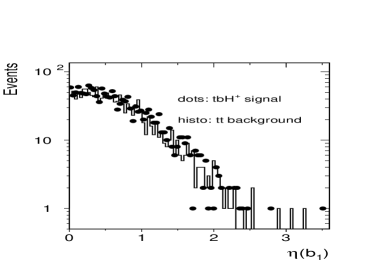
Figure 2: Left: $\eta$ distribution of leading (most energetic) $b$ quark jet. Right: $\eta$ distribution of second (least energetic) $b$ quark jet.

 

Figure 3: Left: $\eta$ distribution of leading light quark jet. Right: $\eta$ distribution of second light quark jet.

 

Figure 4: Left: spatial distance $d(\tau,b_{1})=\sqrt{(\phi(\tau)-\phi(b_{1}))^{2}+(\eta(\tau)-\eta(b_{1}))^{2}}$, where $\phi$ (in rad) is the azimuthal angle, between tau and leading $b$ quark jet. Right: spatial distance $d(\tau,b_{2})$ between tau and second $b$ quark jet.

 

Figure 5: Left: spatial distance $d(\tau,j_{1})$ between tau and leading light quark quark jet. Right: spatial distance $d(\tau,j_{2})$ between tau and second light quark jet.

 

Figure 6: Left: $H$ distribution per event, where $H=H({\rm jets})+P_{t}(\tau)$. Right: $H({\rm jets}$), where $H({\rm jets})=\sum P^{\rm jet}_{t}$.

 

Figure 7: Left: invariant mass of $b$ quark jets. Right: invariant mass of light quark jets.

 

Figure 8: Left: invariant mass of two light quark jets and the leading $b$ quark jet. Right: invariant mass of two light quark jets and the second $b$ quark jet.

 

Figure 9: Left: $S_{\mathrm{hat}}=\sqrt{(p_{\Sigma}^{4})^{2}-(\vec{p}_{\Sigma})^{2}}$ distribution, where $p_{\Sigma}=p_{b_{1}}+p_{b_{2}}+p_{j_{1}}+p_{j_{2}}+p_{\tau}$. Right: missing $p_{t}$ of the event.

3 OUTLOOK AT THE LHC

As at the Tevatron, the search strategies at the LHC depend on the charged Higgs boson mass. If $m_{H^{\pm}}<m_{t}-m_{b}$ (latter referred to as a light Higgs boson), the charged Higgs boson can be produced in top (anti-)quark decay. The main source of top (anti-)quark production at the LHC is $t\bar{t}$ pair production ($\sigma_{t\bar{t}}=850$ pb at NLO) [596]. For the whole ($\tan\beta,m_{A}$) parameter space there is a competition between the $bW^{\pm}$ and $bH^{\pm}$ channels in top decay keeping the sum $\mathrm{BR}(t\to bW^{+})+\mathrm{BR}(t\to bH^{+})$ at almost unity. The top quark decay to $bW^{\pm}$ is however the dominant mode for most of the parameter space. Thus, the best way to search for a (light) charged Higgs boson is by requiring that the top quark produced in the $tbH^{\pm}$ process decays to a $W$. While in the case of $H^{\pm}$ decays $\tau$’s will be tagged via their hadronic decay producing low-multiplicity narrow jets in the detector, there are two different $W$ decays that can be explored. The leptonic signature $b\bar{b}H^{\pm}W^{\mp}\to b\bar{b}\tau\nu l\nu$ provides a clean selection of the signal via the identification of the lepton $l=e,\mu$ but the charged Higgs transverse mass cannot be reconstructed because of the presence of two neutrinos with different origin. In this channel charged Higgs discovery will be determined by the observation of an excess of such events over SM expectations through a simple counting experiment. In the case of hadronic decays $b\bar{b}H^{\pm}W^{\mp}\to b\bar{b}\tau\nu jj$ the transverse mass can instead be reconstructed since all neutrinos are arising from the charged Higgs boson decay. This allows for an efficient separation of the signal and the main $t\bar{t}\to b\bar{b}W^{\pm}W^{\mp}\to b\bar{b}\tau\nu jj$ background (assuming $m_{H^{\pm}}\lower 3.01385pt\hbox{$\;\stackrel{{\scriptstyle\textstyle>}}{{\sim}}\;$}m_{W}$). The absence of a lepton ($e$ or $\mu$) provides a less clean environment but the use of the transverse mass makes it possible to reach the same mass discovery region as in the previous case and also to extract the charged Higgs boson mass. Both these channels show that after an integrated luminosity of 30 fb^-1 the discovery could be possible up to a mass of 150 GeV for all tan$\beta$ values in both ATLAS and CMS [597, 598].

If the charged Higgs is heavier than the top quark, the dominant channels are $H^{\pm}\to\tau\nu$ and $H^{\pm}\to tb$. They have both been studied by ATLAS and CMS [599, 600, 601, 602]. The charged Higgs bosons are produced in the $pp\to tbH^{\pm}$ channel. For the $H^{\pm}\to tb$ decay, a charged Higgs boson can be discovered up to high masses ($m_{H^{\pm}}\sim 400$ GeV) in the case of very large $\tan\beta$ values and this reach cannot be much improved because of the large multi-jet environment. For the $H^{\pm}\to\tau\nu$ decay mode this reach is larger due to a cleaner signal despite a lower branching ratio. In this case the 5$\sigma$ reach ranges from $\tan\beta=20$ for $m_{H^{\pm}}=200$ GeV to $\tan\beta=30$ for $m_{H^{\pm}}=400$ GeV.

For the LHC, signal and background events have been simulated in the same way as for the Tevatron as explained in Sec. 2, using PYTHIA, version 6.325, with the factorization scale $(m_{t}+m_{H^{\pm}})/4$, the renormalization scale $m_{H^{\pm}}$, and the running $b$-quark mass evaluated at $m_{H^{\pm}}$. Table 2 lists the resulting theoretical cross sections, and the cross sections with the basic cut $P_{t}^{\rm jet}>5$ GeV applied. The LHC rates allow for the discovery to be less challenging than at the Tevatron in the region $m_{H^{\pm}}\sim m_{W^{\pm}}$, yet the separation of signal events from background remains crucial for the measurement of the charged Higgs mass.

Table 2: LHC cross sections of background $q\bar{q},gg\to t\bar{t}$ and signal $q\bar{q},gg\to tbH^{\pm}$ for $\tan\beta=30$ and $m_{H^{\pm}}=80,100$ and $160$ GeV into the final state $2b+2j+\tau_{\mathrm{jet}}+\not\!P_{t}$ before ($\sigma^{\rm th}$) and after ($\sigma$) the basic cut of $P_{t}>5$ GeV for all jets after smearing of the momenta as decribed in the text has been applied.

	$q\bar{q},gg\to t\bar{t}$	$q\bar{q},gg\to tbH^{\pm}$
	$m_{H^{\pm}}=80$ GeV	$m_{H^{\pm}}=80$ GeV	$m_{H^{\pm}}=100$ GeV	$m_{H^{\pm}}=160$ GeV
$\sigma^{\rm th}$ (pb)	44.9	73.1	51.1	4.4
$\sigma$ (pb)	40.0	68.8	47.8	4.0

The LHC kinematic distributions are shown in detail in Figs. 10–18. The choice of variables is identical to the one for the Tevatron and allows for a one-to-one comparison, the differences being due to a change in CM energy (and to a somewhat lesser extent, leading partonic mode). The main differences with respect to Figs. 1–9 are that all the $\eta$ distributions extend to larger values and that the various invariant masses have longer high energy tails. As for similarities, it should be noted that the effect of the spin differences between $W$ and $H^{\pm}$ events can only be explored for the $P_{t}$ spectrum of the $\tau$ jet. These observations lead to the conclusion that the same method of “Optimal Observables” can be used to separate signal from background at both the Tevatron and the LHC.

 

Figure 10: Left: $P_{t}$ of the tau-jet. Right: $\eta$ distribution of the tau-jet.

 

Figure 11: Left: $\eta$ distribution of leading $b$ quark jet. Right: $\eta$ distribution of second $b$ quark jet.

 

Figure 12: Left: $\eta$ distribution of leading light quark jet. Right: $\eta$ distribution of second light quark jet.

 

Figure 13: Left: spatial distance $d(\tau,b_{1})=\sqrt{(\phi(\tau)-\phi(b_{1}))^{2}+(\eta(\tau)-\eta(b_{1}))^{2}}$, where $\phi$ (in rad) is the azimuthal angle, between tau and leading $b$ quark jet. Right: spatial distance $d(\tau,b_{2})$ between tau and second $b$ quark jet.

 

Figure 14: Left: spatial distance $d(\tau,j_{1})$ between tau and leading light quark quark jet. Right: spatial distance $d(\tau,j_{2})$ between tau and second light quark jet.

 

Figure 15: Left: $H$ distribution per event, where $H=H({\rm jets})+P_{t}(\tau)$. Right: $H({\rm jets}$), where $H({\rm jets})=\sum P^{\rm jet}_{t}$.

 

Figure 16: Left: invariant mass of $b$ quark jets. Right: invariant mass of light quark jets.

 

Figure 17: Left: invariant mass of two light quark jets and the leading $b$ quark jet. Right: invariant mass of two light quark jets and the second $b$ quark jet.

 

Figure 18: Left: $S_{\mathrm{hat}}=\sqrt{(p_{\Sigma}^{4})^{2}-(\vec{p}_{\Sigma})^{2}}$ distribution, where $p_{\Sigma}=p_{b_{1}}+p_{b_{2}}+p_{j_{1}}+p_{j_{2}}+p_{\tau}$. Right: missing $p_{t}$ of the event.

4 CONCLUSIONS

The discovery of charged Higgs bosons can shed light on the possible existence of a Higgs mechanism beyond the SM. We have studied charged Higgs boson topologies produced at the current Tevatron and the future LHC energies. While sizable differences between signal and background are expected whenever $m_{H^{\pm}}\neq m_{W}$, near the current mass limit of about $m_{H^{\pm}}\approx 80$ GeV the kinematic spectra are very similar between SM $t\bar{t}$ decays and those involving charged Higgs bosons. For this mass spin information will however help to distinguish between signal and background. Characteristic differences of the kinematic distributions between signal and background at both the Tevatron and LHC were discussed and the method of “Optimal Observables” has been emphasized as a generic analysis tool explorable at both accelerators. Future studies will address the spin correlation issue in more detail. Independent of the kinematic behavior, the identification of a hadronic tau-lepton will be an experimental challenge in an environment with typically four jets being present.

Acknowledgements

We would like to thank the Les Houches conference organizers for their kind invitation and Johan Alwall for fruitful discussions.

Part 31 Diphoton production at the LHC in the RS model

S. Ferrag, O. Jinnouchi and K. Sridhar

The past decade has been a phase of intense theoretical activity in the area of extra space dimensions and the resurgence of interest in the physics of extra dimensions is due to the new paradigm of brane-worlds. For high energy physics this new pardigm is exciting because it provides fresh perspectives to the solution of the hierarchy problem and also suggests the discovery of new physics at TeV-scale colliders.

In an attempt to find a genuine solution to the hierarchy problem Randall and Sundrum discovered a model now known in the literature as the Randall-Sundrum model or the RS model [470]. In the RS model, one starts with a five-dimensional spacetime where the fifth dimension $\phi$ is compactified on a ${\bf S}^{1}/{\bf Z^{2}}$ orbifold with a radius $R_{c}$ such that $R_{c}^{-1}$ is somewhat smaller than $M_{P}$, the Planck length. Two D3-branes called the Planck brane and the TeV brane are located at $\phi=0,\ \pi$, the orbifold fixed points and the SM fields are localised on the TeV brane. With a five-dimensional metric of the form

$$ds^{2}=e^{-{\cal K}R_{c}\phi}\eta_{\mu\nu}dx^{\mu}dx^{\nu}\leavevmode\nobreak\ +\leavevmode\nobreak\ R_{c}^{2}d\phi^{2}.$$ (1)

the model provides a novel solution to the hierarchy problem. Here $K$ is a mass scale related to the curvature. The warp factor acts as a conformal factor for the fields localised on the brane and mass factors get rescaled by this factor. So $M_{P}=10^{19}$ GeV for the Planck brane at $\phi=0$ gets rescaled to $M_{P}{\rm exp}(-KR_{c}\pi)$ for the TeV brane at $\phi=\pi$. The warp factor generates $\frac{M_{P}}{M_{EW}}\sim 10^{15}$ by an exponent of order 30 and solves the hierarchy problem. In order to solve the dynamical problem of stabilising $R_{c}$ against quantum fluctuations a scalar field in the bulk [603, 604, 605, 606] with a stabilising potential is introduced.

On compactification of the fifth dimension, a tower of massive Kaluza-Klein (KK) excitations of the graviton, $h^{(\vec{n})}_{\mu\nu}$, result on the TeV brane where it interacts with the SM particles by:

$${\cal L}_{int} = -\frac{1}{\overline{M}_{P}}T^{\mu\nu}(x)h^{(0)}_{\mu\nu}(x)-\frac{e^{\pi{\cal K}R_{c}}}{\overline{M}_{P}}\sum_{1}^{\infty}T^{\mu\nu}(x)h^{(n)}_{\mu\nu}(x)\ ,$$ (2)

where $\overline{M}_{P}=M_{P}/\sqrt{8\pi}$ is the reduced Planck mass and $T^{\mu\nu}$ is the energy-momentum tensor for the SM particles. The masses of the $h^{(\vec{n})}_{\mu\nu}$ are given by

$$M_{n} = x_{n}{\cal K}\leavevmode\nobreak\ e^{-\pi{\cal K}R_{c}}$$ (3)

where the $x_{n}$ are the zeros of the Bessel function $J_{1}(x)$ of order unity [605, 606]. The resulting masses of the KK gravitons are not evenly spaced but appear at the Bessel zeroes. The graviton zero-mode couples with a $1/\overline{M}_{P}$ strength and essentially decouples but the couplings of the massive gravitons are enhanced by the exponential $e^{\pi{\cal K}R_{c}}$ leading to interactions of electroweak strength.

The basic parameters of the RS model are

$$m_{0} = {\cal K}e^{-\pi{\cal K}R_{c}}$$

$$c_{0} = {\cal K}/M_{P}$$ (4)

where $m_{0}$ is a scale of the dimension of mass and sets the scale for the masses of the KK excitations, and $c_{0}$ is an effective coupling. It is expected that the parameter $c_{0}$ lies in the range [0.01, 0.1]. The upper bound on $c_{0}$ results from requiring that ${\cal K}$ is not too large so as to avoid strong curvature effects and the lower bound ensures that ${\cal K}$ is not too small as compared to $\overline{M}_{P}$, since that would introduce a new hierarchy. Values of $m_{0}$ are determined in terms of ${\cal K}R_{c}\sim 10$, so that $m_{0}$ ranging from about a 100 GeV to a TeV are possible. Again, avoidance of strong curvature effects suggests that the mass of the first RS graviton is not too much more than a TeV.

Because of the fact that the zero mode decouples, it is only the heavier modes one can hope to detect in experiments. In the fortuitous circumstance that these modes are within the reach of high-energy experiments, interesting effects like resonance production can be observed, with the resonance decaying within the detectors. If this is not the case and if the the gravitons are heavier then the best strategy will be to look for the virtual effects of the gravitons on observables measured in high-energy collider experiments.

In this paper, we study the virtual effects of the exchange of spin-2 KK modes, in the RS model, in diphoton production at the LHC. The cross-sections for the $q\bar{q}\rightarrow\gamma\gamma$ and $gg\rightarrow\gamma\gamma$ subprocesses are [607, 608]:

$$\frac{d\hat{\sigma}}{d\hat{t}}(q\bar{q}\rightarrow\gamma\gamma) = \frac{2\pi\alpha^{2}Q_{q}^{4}}{3\hat{s}^{2}}\frac{1+{\rm cos}^{2}\theta^{*}}{1-{\rm cos}^{2}\theta^{*}}$$ (6)

$$+\frac{\alpha Q_{q}^{2}}{96\pi}{\rm Re}[C(x_{s})](1+{\rm cos}^{2}\theta^{*})+\frac{s^{2}}{24576\pi}|C(x_{s})|^{2}(1-{\rm cos}^{4}\theta^{*}),$$

and

$$\frac{d\hat{\sigma}}{d\hat{t}}(gg\rightarrow\gamma\gamma) = +\frac{s^{2}}{65536\pi}|C(x_{s})|^{2}(1+6{\rm cos}^{2}\theta^{*}+{\rm cos}^{4}\theta^{*}).$$ (7)

The SM box contribution $gg\rightarrow\gamma\gamma$ can be neglected because even though at the LHC, this box contribution is somewhat increased because of the initial gluon flux but, as shown in Ref. [608], in spite of this increase this contribution is an order of magnitude smaller than the SM $q\bar{q}\rightarrow\gamma\gamma$ contribution for diphoton invariant mass of 500 GeV and is more than two orders of magnitude smaller for diphoton invariant mass greater than about 1750 GeV. On the other hand, the new physics effects dominate in the large invariant mass bins and, therefore, in the invariant mass region of interest the SM box contribution is negligible even for the case of the LHC.

In the above equations, ${\rm cos}\theta^{*}$ is the scattering angle in the partonic c.m. frame, $x_{s}\equiv\frac{\sqrt{\hat{s}}}{m_{0}}$ and $C(x)$ is defined as

$$C(x) = \frac{32\pi c_{0}^{2}}{m_{0}^{4}}\lambda(x)$$ (8)

with

$$\lambda(x_{s}) = m_{0}^{2}\sum_{n}\frac{1}{\hat{s}-M_{n}^{2}+iM_{n}\Gamma_{n}}\ .$$ (9)

and the $M_{n}$ are the masses of the individual resonances and the $\Gamma_{n}$ are the corresponding widths. The graviton widths are obtained by calculating their decays into final states involving SM particles. This gives

$$\Gamma_{n}=m_{0}c_{0}^{2}x_{n}^{3}\Delta_{n}$$ (10)

where

$$\Delta_{n}=\Delta_{n}^{\gamma\gamma}+\Delta_{n}^{gg}+\Delta_{n}^{WW}+\Delta_{n}^{ZZ}+\sum_{\nu}\Delta_{n}^{\nu\nu}+\sum_{l}\Delta_{n}^{ll}+\sum_{q}\Delta_{n}^{qq}+\Delta_{n}^{HH}$$ (11)

and each $\Delta_{n}^{aa}$ is a numerical coefficient arising in the decay $h^{n}\to a\bar{a}$. For the partial width $\Delta_{n}^{HH}$, we have fixed $M_{H}=250$ GeV in our numerical studies. We point out that our results are very insensitive to the choice of $M_{H}$.

Given the masses and the widths of the individual graviton resonances, we have to sum over all the resonances to get the value of $\lambda(x_{s})$. We perform this sum numerically, using the fact that the higher zeros of the Bessel function become evenly-spaced.

The above sub-process cross sections are privately implemented in the matrix element of the PYTHIA [46] code in conjunction with the Standard Model diphoton production sup-processes, $q\bar{q}\rightarrow\gamma\gamma$ and $gg\rightarrow\gamma\gamma$. The interference of newly implemented graviton resonances with the Standard Model processes are then inevitably taken into account in this study. In the first part of the study, events including the graviton resonance masses from lowest to higher are produced. The generated events are passed through the ATLAS fast detector simulation (ATLFAST [18]) and the resonance widths and positions for several sets of parameters are assessed under 100fb^-1 integrated luminosity. In the second part, our study is devoted for illustrating the physics potential rearch, where the production and measurements of only the lightest gravition resonance is considered under 10fb^-1 luminisity, simulating the early LHC period. In this study, the center of mass energy of LHC (14TeV) is assumed, parametrizations of the CTEQ6M parton distribution function [47] are used throughout the study. ATLFAST, ver.2.53 is used to give the realistic estimation of the resonance measurements. The standard detector response parameters are used. Particularly for photon detection, the kinetic acceptance of Et $>50$ GeV and $|\eta|<2.5$ is assumed. The isolatetd photons are separated by $\Delta R>0.4$ from other clusters and Et $<10$ GeV in a cone $\Delta R=0.2$ around the photon is required. Identification efficiency are assumed to be 1.0. Followings are the first part of the fast simulation study, aiming at getting the characteristics of the distributions implemented RS resonances. Figure 1 and fig. 2 show the diphoton invariant mass distribution, $d\sigma/dM$, and the angle distribution, $d\sigma/d\cos\theta^{*}$, respectively. Three sets of the basic RS model parameters, $(m_{0},c_{0})$ = (150GeV, 0.01), (150GeV,0.03), (300GeV,0.01), are chosen and shown with different colored lines, along with the Standard Model diphoton distribution (in black). In the invariant mass plot, as expected from the equations above, the $m_{0}$ parameter has a direct relation to the resonance position, while the $c_{0}$ has a strong correlation to the width of the resonances. The interference term contributions are expected to be enhanced around the resonance, however size of the interferences are found to be fairly small, and it will be hard to observe experimentally.

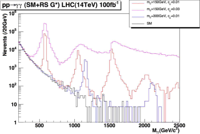
Figure 1: Diphoton invariant mass distributions for arbitrary selected RS model parameters and Standard Model as a reference. Vertical axis represents number of events expected at 100 $fb^{-1}$

In the angle distribution, the shape is clearly distinguished from the Standard Model distribution. The RS model resonances contribute to more in central ($\theta^{*}\sim 0$) than SM in the particle scattering c.m. frame.

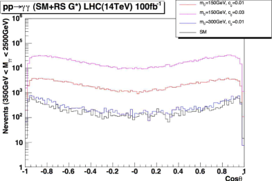
Figure 2: Angle distributions for the sets of RS model parameters and Standard Model as a reference. Note that $M_{\gamma\gamma}$ cut is applied for event selection (2500GeV$>M_{\gamma\gamma}>$350GeV).

In the second part, the physics discovery reach is assessed upon the assumed integrated luminosity of 10 fb^-1 at LHC ATLAS. The RS model parameter space (the region $m_{0}=0.005-0.05$, $c_{0}=$150-1000GeV) is surveyed and the signal significance for the each point is estimated. Only the lightest invariant mass resonance is considered here. The number of events of signal and background are estimated by fitting the invariant mass distribution with the function, Standard Model + Resonance, in more specific, $f(M)=P_{0}\cdot M^{-P_{1}}+P_{2}\cdot M\cdot\mbox{Breit Wigner}(M,P_{3},P_{4})$, where $P_{0}$ and $P_{1}$ are fixed by fitting the pure Standard Model distribution in order to reduce the instability of the resonance fit. $P_{2}$ represents the scale correction parameter for the resonance, $P_{3}$, $P_{4}$ are the mean and width values of Breit Wigner function respectively. Figure 3 shows the typical fit result at $m_{0}=300$ GeV, $c_{0}=0.01$ point. The signal region is defined as the $\pm 3\sigma$ from the Breit Wigner centroid. The number of events within this region ($N_{obs}$) and the expected background level from Standard Model ($N_{SM}$) are used to estimate the signal significance, $N_{signal}/\sqrt{N_{BG}}$, where $N_{signal}=N_{obs}-N_{SM}$ and $N_{BG}=N_{SM}$. In case the resonance width is too thin ($\sigma<5GeV$), $\pm 15$ GeV is used instead of $\pm 3\sigma$ cut. In the domain where $m_{0}>600$ GeV, a fit procedure becomes very unstable due to the small resonance signal. As a practical solution, the region $\pm 100$ GeV from the expected resonance position ($m_{0}\times 3.83$) is used instead.

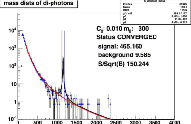
Figure 3: Typical fitting result defined as in the context. Standard Model contribution is fixed during the fitting procedure, and shown as the smooth red curve in the plot. Data points are normalized to $10fb^{-1}$, drawn with blue points. Breit Wigner fit is drawn with black function. Parallel blue vertical lines are the integral region ($\pm 3\sigma$) for the significance estimation.

Figure 4 is the contour distribution of the basic RS model parameters, $m_{0},c_{0}$ showing the signal significance in Z-axis with logarithmic scale. The boundary, $S/\sqrt{B}=3$, is presented with a thick black curve, showing the physics descovery reach at 10 fb^-1 luminosity.

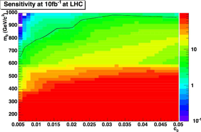
Figure 4: Signal significance distribution in $m_{0}-c_{0}$ parameter phase space. The black curve shows the expected discovery sensitivity boundary ($S/\sqrt{B}=3$).

To summarize, we have investigated the effects of the interactions of the spin-2 Kaluza-Klein modes with SM fields in diphoton production at the LHC, in the context of the Randall-Sundrum model. Process cross-section is implemented in PYTHIA code, and detector effect is simulated with ATLFAST. Interference term between KK resonances and Standard Model process is found to be negligible. Signal significance is estimated using the invariant mass distributions of the photon pair. $S/\sqrt{B}=3$ reach at 10 fb^-1 integrated luminosity is extracted from the $m_{0}-c_{0}$ parameter phase space.

Part 32 Higgsless models of electroweak symmetry breaking

G. Cacciapaglia

1 INTRODUCTION

The main theoretical prejudice against field theories with fundamental scalars, like the Higgs boson in the Standard Model, is the instability of their mass. If there is not any symmetry protecting it, the radiative corrections to the mass parameter will be proportional to the cutoff, or to the scale where new physics has to be added to the theory. Thus, unless a large fine tuning is invoked, the SM description of EWSB is not satisfactory. The most radical approach to this problem is to built a theory where there is not any light scalar in the low energy spectrum, or Higgsless models.

If we remove the Higgs from the SM, the first problem we run into is the scattering of the longitudinally polarized $W$ bosons: the tree level amplitude grows like the energy square and at some energy scale (around $1.8$ TeV in the SM) we lose control of the perturbation expansion. The role of the Higgs is to cancel such divergent term. Historically, the first approach was to assume that strong coupling indeed occurs around $1$ TeV, and that it is the strong dynamics itself to induce the gauge symmetry breaking: this is the idea of technicolour. However, these models have serious problems in accommodating the electroweak precision tests performed at LEP in the last decade: generically they predict large deviations, and the lack of calculability does not allow to decide if this scenario is definitely ruled out. Is it possible to build a Higgsless model where the loss of perturbative control occurs at energies larger that a TeV? The easiest possibility is to add a massive vector particle, with mass in the TeV range, that cancels the quadratically growing term in the scattering amplitude. However, the scattering amplitude of the new heavy boson will grow quadratically in the energy again, thus incurring in a strong coupling regime at a higher energy than before. If we want to keep playing this game, we can add another massive vector boson, and so on. The cancellation of the growing terms in the amplitude will impose sum rules on the couplings and masses of the new heavy states. For instance, from the $W_{L}\,W_{L}$ scattering:

$$g_{WWWW} = e^{2}+g_{WWZ}^{2}+\sum_{k}g_{WWk}^{2}\,;$$ (1)

$$g_{WWWW} = \frac{3}{4}\left(g_{WWZ}^{2}\frac{M_{Z}^{2}}{M_{W}^{2}}+\sum_{k}g_{WWk}^{2}\frac{M_{k}^{2}}{M_{W}^{2}}\right)\,.$$ (2)

The first sum rule ensures the cancellation of a term growing with the fourth power of the energy, whose cancellation in the SM is ensured by gauge invariance that relates the couplings. In Refs. [609, 610, 611, 612, 613, 614, 615, 616], it has been shown that these sum rules are automatically satisfied in Yang-Mills theories in extra dimensional spaces, where the gauge symmetries are broken by suitable boundary conditions. Namely, one can impose that the gauge fields associated with the broken generators vanish on the boundaries of the extra dimension, so that all the modes associated with such fields are massive. It is also possible to write 4 dimensional theories with the same property: these are the so called moose models, or deconstructed extra dimensions [488]. The idea is to latticize the extra dimension, and replace it with a finite number of replicas of the gauge group. Scalar links will provide the breaking of the $N$ gauge groups. Higgsless models have been proposed both in the 5 dimensional case in Refs. [550, 617, 618], and further studied in Refs. [619, 620, 621, 622, 556, 623, 624, 625], and in 4 dimensions in Refs. [626, 627, 628] (see also Refs. [629, 630, 631, 632, 633, 634, 635, 636, 637, 638, 639, 640, 641, 642]). In the rest of this review, we will focus on the extra dimensional attempts, however, the same conclusions apply to the 4 dimensional models. The only difference is that the deconstructed models are less constrained, as they explicitly violate 5D Lorentz invariance.

1.1 A ONE PAGE MINICOURSE IN EXTRA DIMENSIONS

If we were to consider the existence of an extra spatial dimension, in order to hide it at low energies we need to compactify it, so that it will be negligible at energies below its typical length. The simplest way to imagine it, is to think in terms of an interval. Any field $\Phi$ will also depend on the extra coordinate $z$: we can reduce the theory to a 4 dimensional one if we Fourier expand the fields in the extra component, namely

$$\Phi(x_{\mu},z)=\sum_{k}f_{k}(z)\phi_{k}(x_{\mu})\,;$$ (3)

where a 4D field $\phi_{k}$ is associated to each frequency of the interval. The mass $m_{k}$ of these infinite fields will be determined by the boundary conditions at the interval endpoints, and are like the energy required to excite that particular frequency.

In order to make this statement more clear, we will focus on a simple gauge theory in a flat extra dimension. In this case, the 5D vector has an extra component along the extra direction

$$A=(A_{\mu},A_{5})\,.$$ (4)

However, not all the modes in the 4D scalar $A_{5}$ are physical: indeed they can be gauged away, and they will play the role of the longitudinal modes of the massive vectors resulting from the 4D reduction described above. The simplest boundary condition that can be imposed on this system are Neumann, namely the vanishing of the derivative along the extra component on the interval endpoints $\partial_{5}A_{\mu}=0$. These BCs allows for a constant solution $f_{0}=\mbox{const}$, that corresponds to a massless vector . From the 4D point of view, the bulk gauge symmetry is unbroken. The massive states will have masses given by $n/L$, $L$ being the length of the interval and $n$ an integer.

Another possibility is to impose Dirichlet BCs for the vector components: in this case the flat solution is not allowed and all the vector states are massive. This signals that the gauge symmetry is also broken in 4D. However, the choice of BCs is not completely arbitrary, as not all the possibilities will lead to a unitary theory: the sum rules advocated above will be satisfied only for a healthy choice. It turns out that healthy BCs come from a spontaneous breaking of the symmetry on the boundaries. In order to see it, we can add to the theory a scalar degree of freedom localized on one of the two endpoints, and assume that it will develop a vacuum expectation value as for the SM Higgs. The Neumann BC will be modified to:

$$\partial_{5}A_{\mu}\pm g^{2}\frac{v^{2}}{4}A_{\mu}=0\,,$$ (5)

where $v$ is the VEV and the sign corresponds to the choice of endpoint. For small VEV, the mass of the gauge boson is proportional to $gv$. However, in the limit of large $v$, the mass of the first massive state is given by $1/(2L)$: this corresponds to switching the BC to Dirichlet BCs. If we play this trick on both the endpoints, the first state will have mass $1/L$, however in this case the BCs for $A_{5}$ will allow for a scalar massless state that cannot be gauged away. Indeed, we are breaking the symmetry twice, with two separate Higgs sectors: thus only one combination of the two resulting goldstone bosons is eaten by the massive vectors, the other one is a physical massless scalar.

2 THE MODEL

We will consider the model proposed in Refs. [550, 623]: a SU(2)${}_{L}\times$SU(2)${}_{R}\times$U(1)_B-L gauge theory on a AdS₅ background, i.e. one extra dimension with a warped metric [470]. The conformally flat metric on AdS can be parametrized as:

$$ds^{2}=\left(\frac{R}{z}\right)^{2}\left(\eta_{\mu\nu}dx^{\mu}dx^{\nu}-dz^{2}\right)\,,$$ (6)

where the extra coordinate $z$ is on the interval $[R,R^{\prime}]$. The curvature $R$ is usually assumed to be of order $1/M_{Pl}$, but in this case it will be a free adjustable parameter. The physical interpretation of this metric is that the unit length, or equivalently the energy scale, depends on the position in the extra dimension. On the $z=R$ endpoint, the Planck brane, it is of order $1/R$, while on the $z=R^{\prime}$ endpoint, the TeV brane, it is warped down to the smaller scale $1/R^{\prime}$, that we will assume to be of order the weak scale. The bulk gauge symmetry is broken on the boundaries of the extra dimension: on the Planck brane we will preserve the SM gauge group, so that the breaking pattern is SU(2)${}_{R}\times$U(1)${}_{B-L}\to$ U(1)_Y. On the TeV brane, on the other hand, we will break the two SU(2)’s to the diagonal one SU(2)${}_{L}\times$SU(2)${}_{R}\to$SU(2)_D . As already mentioned, the breaking is realized imposing Dirichlet BC’s for the broken generators . If we call $g_{5}$ and $\tilde{g}_{5}$ the gauge couplings of the two SU(2)’s and of the U(1), the BC’s are [550]:

$${\rm at}\ z=R^{\prime}: \left\{\begin{array}[]{l}\partial_{z}(A^{L\,a}_{\mu}+A^{R\,a}_{\mu})=0\,,\\ A^{L\,a}_{\mu}-A^{R\,a}_{\mu}=0,\ \partial_{z}B_{\mu}=0\,;\end{array}\right.$$ (9)

$${\rm at}\ z=R: \left\{\begin{array}[]{l}\partial_{z}A^{L\,a}_{\mu}=0\,,\\ \partial_{z}(g_{5}B_{\mu}+\tilde{g}_{5}A^{R\,3}_{\mu})=0\,,\\ \tilde{g}_{5}B_{\mu}-g_{5}A^{R\,3}_{\mu}=0\,.\end{array}\right.$$ (13)

where $A^{L}$, $A^{R}$ and $B$ are the gauge fields respectively of SU(2)_L, SU(2)_R and U(1)_B-L. These boundary conditions allow to expand the gauge fields as follows:

$$\left\{\begin{array}[]{rcl}A_{\mu}^{L3}&=&\frac{1}{g_{5}}a_{0}\gamma_{\mu}+\sum_{k=1}^{\infty}\psi_{k}^{(L3)}(z)Z_{\mu}^{(k)}(x)\,,\\ A_{\mu}^{R3}&=&\frac{1}{g_{5}}a_{0}\gamma_{\mu}+\sum_{k=1}^{\infty}\psi_{k}^{(R3)}(z)Z_{\mu}^{(k)}(x)\,,\\ A_{\mu}^{B}&=&\frac{1}{\tilde{g}_{5}}a_{0}\gamma_{\mu}+\sum_{k=1}^{\infty}\psi_{k}^{(B)}(z)Z_{\mu}^{(k)}(x)\,;\end{array}\right.\quad\left\{\begin{array}[]{rcl}A_{\mu}^{L\pm}&=&\sum_{k=1}^{\infty}\psi_{k}^{(L\pm)}(z)W_{\mu}^{(k)\pm}(x)\,,\\ A_{\mu}^{R\pm}&=&\sum_{k=1}^{\infty}\psi_{k}^{(R\pm)}(z)W_{\mu}^{(k)\pm}(x)\,;\end{array}\right.$$ (14)

where the wave functions are combinations of Bessel functions (due to the bulk equation of motion), and the BC’s will fix the spectrum. Note the presence of a flat massless state: this corresponds to the gauge boson of the unbroken U(1)_em, the photon. We also want to identify the lightest massive states, namely $W^{(1)}$ and $Z^{(1)}$, with the SM $W$ and $Z$.

The main reason for working in this non trivial background is twofold: first of all the warping allows to split the masses of the first resonance, that we want to identify with the $W$ and $Z$ bosons, and the other KK states. Indeed, we find that:

$$M_{W}^{2}\sim\frac{1}{{R^{\prime}}^{2}\log\frac{R^{\prime}}{R}}\,,\qquad M_{KK}\sim\frac{\mu}{R^{\prime}}\,,$$ (15)

$\mu$ being the zeros of Bessel functions (for the first resonance $\mu\sim 2.4$). So, the scale of the KK masses is given by the energy scale on the TeV brane $1/R^{\prime}$, while the $W$ mass is split with respect to the mass of the resonances by the $\log$ of the two scales $R$ and $R^{\prime}$. Another important reason is the presence of a custodial symmetry in the bulk and on the TeV brane [484]: this implies that the relation between the $W$ and $Z$ mass is preserved at leading order in the log expansion, and corrections to the $\rho$ parameter are very small. This protection would not occur if we formulated the theory in flat space. The $Z$ mass is given by:

$$M_{Z}^{2}\sim\frac{g_{5}^{2}+2\tilde{g}_{5}^{2}}{g_{5}^{2}+\tilde{g}_{5}^{2}}\frac{1}{{R^{\prime}}^{2}\log\frac{R^{\prime}}{R}}=\frac{M_{W}^{2}}{\cos^{2}\theta_{w}}\,.$$ (16)

The coupling of the photon, allows to identify the 4D SM gauge couplings as functions of the 5D parameters:

$$\frac{1}{g^{2}} = \frac{R\log\frac{R^{\prime}}{R}}{g_{5}^{2}}\,,$$ (17)

$$\frac{1}{{g^{\prime}}^{2}} = R\log\frac{R^{\prime}}{R}\,\left(\frac{1}{g_{5}^{2}}+\frac{1}{\tilde{g}_{5}^{2}}\right)\,.$$ (18)

At this point the theory has only 4 parameters: the two energy scales $R$ and $R^{\prime}$, and the two bulk gauge couplings. The only free parameter, not fixed by the SM, is the scale of the resonances $M^{\prime}$. For the moment we will allow this scale to be between $500$ GeV and $1$ TeV, the reason for this choice will be clear later when we discuss the unitarity bounds.

The major stumbling block for any theory beyond the SM is the level of corrections to Electroweak Precision measurements, mainly performed by LEP1 at the Z pole, and by LEP2 [450, 643]. In the following we will focus on the old parametrization by Peskin and Takeuchi [644]: in universal theories the corrections to Z pole observables can be described by only 3 parameters, called $S$, $T$ and $U$. Another kind of corrections are given by 4-fermi operators induced at tree level by the exchange of the massive gauge bosons, and we will comment on them separately . The parameter $U$ is generically small, corresponding to a higher order operator in the effective lagrangean, so we will neglect it. The parameter $T$ can be directly related to the corrections to the relation between the $W$ and $Z$ mass: as already mentioned, the custodial symmetry built in this model will protect this parameter from large corrections. Thus, the parameter $S$ is the worrisome one. In order to compute it, we must specify the fermion content of the theory, as it also depends on the couplings between gauge bosons and light fermions. The simplest choice is to localize the light fermions on the Planck brane [618, 621]: the reason is that the SM gauge group is unbroken there, so we will not introduce non-standard couplings, and eventual flavour changing neutral currents will be suppressed by a large scale $1/R$. In this limit, the leading contribution to $S$ is given by:

$$S\sim\frac{6\pi}{g^{2}\log\frac{R^{\prime}}{R}}=\frac{6\pi}{g^{2}}\,\left(2.4\frac{M_{W}}{M^{\prime}}\right)^{2}\sim 1.9\left(\frac{1\,\mbox{TeV}}{M^{\prime}}\right)^{2}\,.$$ (19)

This value is large and positive, similar to the one found in traditional technicolour theories, and it is too big compared with the experimental limit $|S|\leq 0.3$. A more complete analysis of this model, including the effect of localized terms, shows that precision data highly disfavour the model with localized fermions [232].

The solution to this problem is to relax the assumptions of localized fermions, as proposed in Refs. [623, 628] and further studied in Refs. [625, 636, 637, 638]: this will also have another crucial beneficial effect regarding the direct bounds on light gauge bosons. It has been known for a long time in Randall-Sundrum (RS) models with a Higgs that the effective $S$ parameter is large and negative [645] if the fermions are localized on the TeV brane as originally proposed [470]. When the fermions are localized on the Planck brane the contribution to $S$ is positive, and so for some intermediate localization the $S$ parameter vanishes, as first pointed out for RS models by Agashe et al.[484]. The reason for this is fairly simple. Since the $W$ and $Z$ wave functions are approximately flat, and the gauge KK mode wave functions are orthogonal to them, when the fermion wave functions are also approximately flat the overlap of a gauge KK mode with two fermions will approximately vanish. Since it is the coupling of the gauge KK modes to the fermions that induces a shift in the $S$ parameter, for approximately flat fermion wave functions the $S$ parameter must be small. Note that not only does reducing the coupling to gauge KK modes reduce the $S$ parameter, it also weakens the experimental constraints on the existence of light KK modes. This case of delocalized bulk fermions is not covered by the no–go theorem of [232], since there it was assumed that the fermions are localized on the Planck brane.

In order to quantify these statements, it is sufficient to consider a toy model where all the three families of fermions are massless and have a universal delocalized profile in the bulk [623]. We first briefly review the bulk equation of motion in AdS₅. In 5D fermions are vector-like, so that they contain both a left- and right-handed component:

$$\Psi=\left(\begin{array}[]{c}\chi\\ {\psi}\end{array}\right)\leavevmode\nobreak\ ,$$ (20)

where the boundary conditions can be chosen such that there is a zero mode either in the left–handed (lh) or in the right–handed (rh) component. The wave function of the zero mode will be determined by the bulk mass term, that we parametrize by $c$ in units of $R$. If the zero mode is lh, the solution of the bulk equations of motion is:

$$\chi_{0}=A_{0}\left(\frac{z}{R}\right)^{2-c}\,.$$ (21)

Studying the above profile, it’s easy to show that lh (rh) fermions are localized on the Planck brane if $c>1/2$ ($c<-1/2$), else on the TeV brane, while for $c=1/2$ ($c=-1/2$) the profile is flat.

Now, the gauge couplings of the fermions will depend on the parameter $c$ through the bulk integral of the gauge boson wave functions. For a lh fermion, that transforms under the bulk gauge group as a $2_{L}\times 1_{R}\times q_{B-L}$ representation, it reads:

$$a_{0}\,Q\,\gamma_{\mu}+g_{5}\,\mathcal{I}_{l}^{L\mp}(c)\,T_{L\pm}W^{\mp}_{\mu}+g_{5}\,\mathcal{I}_{l}^{(L3)}(c)\,\left(T_{L3}+\frac{\tilde{g}_{5}\,\mathcal{I}_{l}^{(B)}(c)}{g_{5}\,\mathcal{I}_{l}^{(L3)}(c)}\,\frac{Y}{2}\right)Z_{\mu}\leavevmode\nobreak\ ,$$ (22)

where we have used that $Y/2=Q_{B-L}$ (for $SU(2)_{R}$ singlets) and the electric charge is defined as $Q=Y/2+T_{L3}$, and:

$$\mathcal{I}^{X}_{l}(c)=A_{0}^{2}\,\int_{R}^{R^{\prime}}dz\left(\frac{R}{z}\right)^{2\,c}\,\phi_{1}^{X}(z)\leavevmode\nobreak\ .$$ (23)

Only the electric charge does not depend on the fermion profile, as the massless photon is flat along the extra dimension. However, the couplings to the $W$ and $Z$ are affected in a universal way: the corrections can be cast into the definition of the oblique parameters and yield an effective shift of $S$.

In order to do that, we have to impose the following matching condition between the 4D couplings and the 5D parameters of the theory:

$$\tan^{2}\theta_{W}=\frac{{g^{\prime}}^{2}}{g^{2}}=-\frac{\tilde{g}_{5}\,\mathcal{I}_{l}^{(B)}(c_{L})}{g_{5}\,\mathcal{I}_{l}^{(L3)}(c_{L})}\leavevmode\nobreak\ ,$$ (24)

while the matching of the electric charge remains unaffected:

$$\frac{1}{e^{2}}=\frac{1}{a_{0}^{2}}=\left(\frac{1}{\tilde{g}_{5}^{2}}+\frac{2}{g_{5}^{2}}\right)R\log\frac{R^{\prime}}{R}\leavevmode\nobreak\ .$$ (25)

Now, we can recalculate $S$ taking into account this shift: in the limit where $c\sim 1/2$, so that the fermion profile is almost flat, the leading contributions to $S$ are:

$$S=\frac{2\pi}{g^{2}\,\log\frac{R^{\prime}}{R}}\left(1+(2c-1)\,\log\frac{R^{\prime}}{R}+\mathcal{O}\left((2c-1)^{2}\right)\right)\leavevmode\nobreak\ .$$ (26)

In the flat limit $c=1/2$, $S$ is already suppressed by a factor of 3 with respect to the Planck brane localization case. Moreover, the leading terms cancel out for:

$$c=\frac{1}{2}-\frac{1}{2\,\log\frac{R^{\prime}}{R}}\,.$$ (27)

As already mentioned, the other beneficial effect is that the flatness of the light fermion profiles suppresses the couplings with the KK modes of the gauge bosons. This allows to have light modes, in the above mentioned range $500$ GeV $\div$ $1$ TeV, without generating large 4-fermi operators. The presence of light KK modes is crucial however for the unitarization of the longitudinal $W$ and $Z$ scattering amplitudes [619, 622]: indeed, if their mass is above a TeV, their effect enters too late, and the theory loses its perturbative control at a too low scale. In order to have an estimate of such scale we can use 5D naive dimensional analysis [623]. If we estimate the loop amplitude generated by a 5D diagram, it will be given by:

$$\frac{g_{5}^{2}}{24\pi^{3}}E\,,$$ (28)

where it grows with the energy because the coupling is not dimensionless: we need to add an energy dependence to fix the correct dimensions of the amplitude. At the energy where such contribution is of order one, so the loop contributions are comparable with tree level effects, we lose perturbative control on the theory. This scale is given by :

$$\Lambda_{NDA}\sim\frac{24\pi^{3}}{g_{5}^{2}}\frac{R}{R^{\prime}}\sim\frac{24\pi^{3}}{g^{2}}\frac{1}{R^{\prime}\log\frac{R^{\prime}}{R}}\sim\frac{24\pi^{3}}{g^{2}}\,2.4\,\frac{M_{W}^{2}}{M^{\prime}}\,.$$ (29)

As you can see, the smaller $M^{\prime}$, the higher the scale where the theory is not under control . If $M^{\prime}$ is in the range $0.5\div 1$ TeV, the cut off scale is $5\div 10$ TeV: this range is safe enough to protect the theory from incalculable effects.

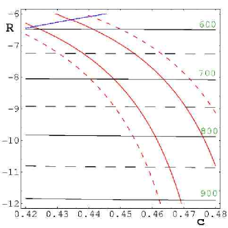
Figure 1: Parameter space region preferred by EWPT: the red lines are the bounds on $|S|\leq 0.25$ ($0.5$ for the dashed lines). Above the blue line, $T$ becomes larger than $0.25$. In black, we also show contour lines for the first KK mass (in GeV), that can be directly related to the strong coupling scale of the model.

In Figure 1 we plotted the preferred parameter space of the theory, choosing as free parameters $c$ and the “Planck” scale $1/R$. The red lines are the bound from $S$: as you can see $S$ prefers a particular value of $c$. Too small values of $1/R$ will induce back a large $T$ parameter (blue line), so that $M^{\prime}\geq 500$ GeV. We also checked that in all the plotted region the effect of 4-fermi operators is negligible.

3 CHALLENGES FOR A MODEL BUILDER

In the previous section we showed how it is possible to cook up a model of Electroweak Symmetry breaking without a Higgs boson. However, before claiming that we have a complete model, there are some more issues that a model builder should address. It is important however to notice that such problems are not related to the electroweak symmetry breaking mechanism itself, but they are more a consequence of the extra dimensional embedding that, as we will see, imposes some generic constraints if we want to introduce fermions in a consistent way.

The first problem arises in the flavour sector. As we already mentioned, a reason for localizing the light generations near the Planck brane is that corrections to Flavour Changing Neutral Currents, coming from higher order operators, should be suppressed by a large scale, of order $1/R$ rather than the strong coupling scale estimated in the previous section. Measurements, indeed, constraint new physics effects to be suppressed by a scale of order $100\div 1000$ TeV. If we delocalize the light fermions, such scale is red shifted to a dangerously low one. In order to escape such bounds, we need to implement a flavour symmetry in the bulk and on the TeV brane. Moreover, the mechanism that generates masses for the fermion themselves will induce some distortions in the wave functions, thus modifying in a non universal way the couplings with the SM gauge bosons. A very brief discussion of these effects can be found in Ref. [623, 628], but a complete study is still missing.

A more serious problem arises when we try to introduce the third family, in particular there is a tension between the heaviness of the top and the coupling of the left-handed $b_{l}$ with the $Z$ boson, that has been measured with a high precision. In a nutshell, the problem is that the $b_{l}$ lives in the same doublet as the $t_{l}$: thus in order to give a large mass to the top, we will inevitably induce large modifications in the wave function of the $b_{l}$. In order to understand the origin of this problem, we need to briefly describe the mechanism that generates masses for fermions [445]. For the third generation quarks, for example, the minimal field content is a SU(2)_L doublet and a SU(2)_R doublet in the bulk:

$$\left(\begin{array}[]{c}\chi_{tL}\\ {\psi}_{tL}\\ \chi_{bL}\\ {\psi}_{bL}\end{array}\right)\ \ \ \left(\begin{array}[]{c}\chi_{tR}\\ {\psi}_{tR}\\ \chi_{bR}\\ {\psi}_{bR}\end{array}\right),$$ (30)

where the $\psi$’s are right handed 4D Weyl spinors, while the $\chi$’s are left handed 4D Weyl spinors. In order to get the correct spectrum, one needs to make sure that the boundary conditions of the $L$ and $R$ fields are different, for example by imposing $(+,+)$ boundary conditions on the $\chi_{tL,bL}$ and $\psi_{tR,bR}$ fields, in order to obtain approximate zero modes, and consequently applying the opposite $(-,-)$ boundary conditions to the remaining fields. A Dirac mass

$$M_{D}R^{\prime}(\chi_{tL}\psi_{tR}+\chi_{bL}\psi_{bR})$$ (31)

can be added on the TeV brane. Due to the remaining $SU(2)_{D}$ gauge symmetry the same term has to be added for top and bottom quarks. The necessary splitting between top and bottom can then be achieved by modifying the BC’s on the Planck brane, where the SU(2)_R is broken: for instance we can add a large brane induced kinetic term for $\psi_{bR}$ [618].

For $c_{L}\sim 0.5$ (or larger) it is impossible to obtain a heavy enough top quark mass. The reason is that for $M_{D}R^{\prime}\gg 1$ the light mode mass saturates at

$$m_{top}^{2}\sim\frac{2}{R^{\prime 2}\log\frac{R^{\prime}}{R}}\,,$$ (32)

which gives for this case $m_{top}\leq\sqrt{2}M_{W}$. Thus one needs to localize the top and the bottom quarks closer to the TeV brane. However, even in this case a sizable Dirac mass term on the TeV brane is needed to obtain a heavy enough top quark. The consequence of this mass term is the boundary condition for the bottom quarks

$$\chi_{bR}=M_{D}R^{\prime}\,\chi_{bL}.$$ (33)

This implies that if $M_{D}R^{\prime}\sim 1$ then the left handed bottom quark has a sizable component also living in an $SU(2)_{R}$ multiplet, which however has a coupling to the $Z$ that is different from the SM value. Thus there will be a large deviation in the $Zb_{l}\bar{b}_{l}$.

A possible way out would be to increase the scale $1/R^{\prime}$: in this way a small $M_{D}R^{\prime}$ should be enough to reproduce the top mass without also inducing large mixings in the b sector [623, 628]. However, in the simple realization the scale of $1/R^{\prime}$ is related to the $W$ mass. A possibility studied in Ref. [624] is to introduce two $R^{\prime}$ scales, one related to the $W$ mass and one to the top mass: this is possible introducing two AdS spaces and matching them on the Planck brane. However, in this scenario a strong coupling will necessarily arise in the top sector, thus affecting the predictive power of the model in the top sector.

Another interesting possibility would be to realize the custodial symmetry in a different way. So far, we assumed that the right-handed components of the top and bottom form a doublet of SU(2)_R. An alternative would be to assume that the $t_{r}$ is a singlet, and the left-handed doublet is part of a bidoublet of SU(2)${}_{L}\times$SU(2)_R. In this way it is possible to write different SU(2)_D invariant masses for the top and bottom on the TeV brane. However, the new BC’s will also give rise to a lighter top, so that it is necessary to localize the fields more closely to the TeV brane.

Another generic problem arising from the large value of the top-quark mass in models with warped extra dimensions comes from the isospin violations in the KK sector of the top and the bottom quarks [472]. If the spectrum of the top and bottom KK modes is not sufficiently degenerate, the loop corrections involving these KK modes to the $T$-parameter could be large. However, the precise value of these corrections crucially depends on how the third generation is realized.

Finally, we should note that this tension in the top sector is really a consequence of the extra dimensional setup. In the deconstructed model of Refs. [642] this problem can be easily solved modifying the couplings of fermions in different points of the lattice points. From the extra dimensional point of view, this would correspond to terms that are not 5D Lorentz invariant.

4 PHENOMENOLOGY AND COLLIDER SIGNATURE

Many different realizations of Higgsless models have been proposed in the literature, differing in the way fermions are introduced and if formulated in an extra dimensional framework or in deconstruction or moose theories. Such models would lead to different experimental signatures. However, the fundamental mechanism that leads to a delay in the scale where the strong coupling breaks the electroweak symmetry is common to all of these models. A model independent prediction is the presence of massive vector bosons that will couple with the $W$ and $Z$ and contribute to the unitarization of the longitudinal mode scattering via sum rules like the ones in Eqs. (1) and (2). Thus, it is possible to identify some signatures at colliders that are typical of Higgsless models, and can be used to probe and discriminate this proposal with respect to other models.

We will again concentrate on the extra dimensional realization of the Higgsless mechanism described above, but the featured pointed here can be easily extended to all the other proposals. In order to have an efficient unitarization, namely a large enough scale of strong coupling, we need the first resonances to be below $1$ TeV. Moreover, their couplings with the SM $W$ and $Z$ have to obey the sum rules: generically the sum rules are satisfied with a high precision by the inclusion of only the first (few) resonances. Another common feature, required by the smallness of oblique corrections, the $S$ parameter, is the smallness of the couplings with the light SM fermions. This observation allows to simplify the phenomenology of the model: indeed we can neglect the couplings with the light fermions, that are model dependent, and only consider the couplings with the gauge bosons. A crucial prediction is again the sum rules: it would be important to measure precisely enough the masses and couplings and check the sum rules. A preliminary study in this direction has been performed in Ref. [647]. The authors focus on the $W-Z$ scattering, because it is easier to measure at hadron colliders. In this channel similar sum rules apply:

$$g_{WWZZ} = g_{WWZ}^{2}\,+\,\sum_{k}g_{WZk}^{2},$$ (34)

$$(g_{WWZZ}-g_{WWZ}^{2})(M_{W}^{2}+M_{Z}^{2})+g_{WWZ}^{2}\,\frac{M_{Z}^{4}}{M_{W}^{2}} = \sum_{k}g_{WZk}^{2}\,\left[3(M^{\pm}_{k})^{2}-\frac{(M_{Z}^{2}-M_{W}^{2})^{2}}{(M^{\pm}_{k})^{2}}\right]\,.$$ (35)

This channel is more appealing because it predicts the presence of charged resonances, and the final state is more easily disentangled from the background.

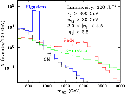
Figure 2: The number of events per 100 GeV bin in the $2j+3l+\nu$ channel at the LHC with an integrated luminosity of 300 fb^-1 and cuts as indicated in the figure. The different histograms correspond to the Higgsless model (blue) with a resonance at $700$ GeV, and two ”unitarization” models: Padé (red) and K-matrix (green). (From Ref. [647])

In Figure 2 we show the number of events expected in a 300 fb^-1 LHC data sample, as a function of the $WZ$ invariant mass $m_{WZ}$. The Higgsless model should be easily seen via a narrow resonance. For comparison, they also studied two unitarization models, relying on strong coupling at a TeV scale. The analysis in the paper shows that, assuming that the production channel is only via gauge boson fusion, LHC at full luminosity should be able to probe all the interesting mass scales for the resonances.

However, at LHC it will not be possible to measure the couplings in order to check the sum rules. A more sophisticated analysis should also include the couplings to the fermions: indeed the Drell-Yan production mechanism should be much more effective. Moreover, the decay channel of the $Z^{\prime}$ in dileptons should make very easy to discover such resonances. As already stresses, such statements depend on the fermion content: as you can see from Figure 1, the smallness of the $S$ parameters highly constraints the parameter space. Thus, if we stick with this minimal model, it should be possible to predict the couplings with fermions, and thus include this effect into the analysis. A combination in the measurements of the decay channels into dileptons and gauge bosons may allow to measure the couplings even at LHC.

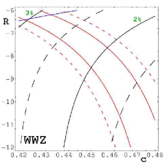
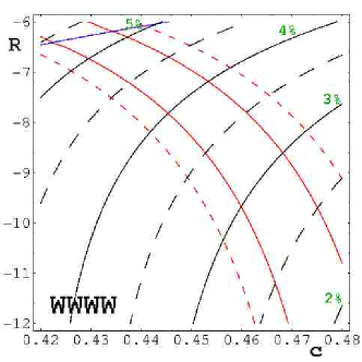
Figure 3: Deviations in the $WWZ$ (left) and $WWWW$ (right) gauge couplings in the Higgsless model as a function of $c$ and $R$. The red and blue lines are the regions preferred by $S$ and $T$, as in Figure 1. The percentage deviation (w.r.t. the SM values) are negative.

Another interesting prediction of Higgsless models is the presence of anomalous 4- and 3-boson couplings. Indeed, in the SM the sum rules canceling the terms growing with the fourth power of the energy are already satisfied by gauge invariance. In order to accommodate the contribution of the new states, the couplings between SM gauge bosons have to be corrected. Assuming that the sum rules are satisfied by the first level it is easy to evaluate such deviations:

$$\frac{\delta g_{WWZ}}{g_{WWZ}}\sim-\frac{1}{2}\frac{M_{W}^{2}}{{M_{Z}^{\prime}}^{2}}-2\Delta\,,\frac{\delta g_{WWWW}}{g_{WWWW}}\sim-\frac{3}{4}\frac{M_{W}^{2}}{{M_{Z}^{\prime}}^{2}}-2\Delta\,;$$ (36)

where $g_{WW1}^{2}/g_{WWWW}\sim 1/4M_{W}^{2}/M_{Z^{\prime}}^{2}+\Delta$ in order to satisfy the second sum rule in Eq. 2.

In Figure 3 we plotted the deviations in the $WWWW$ and $WWZ$ gauge couplings in the Higgsless model described in these proceedings: the red lines encircle the preferred region by EWPTs (as in Figure 1). As you can see, a deviation of order $-1\div 3$ % is expected in the trilinear gauge couplings. This deviation is close to the present experimental bound, coming by measurements at LEP, and might be probed by LHC. A linear collider (ILC) will surely be able to measure such deviations: here we stress again that such deviations are a solid predictions of the Higgsless mechanism and are independent on the details of the specific Higgsless model we are interested in.

5 CONCLUSIONS

The most radical alternative to the SM Higgs mechanism is a theory where gauge symmetry breaking takes place without a scalar particle. In this case, the scattering amplitude of longitudinal modes is unitarized by the presence of a tower of massive vector bosons. Such mechanism naturally arises in extra dimensional theories, where the gauge symmetry breaking is induced by the boundary conditions of gauge fields. The most realistic of such models is embedded in a warped background, thus ensuring a splitting between the $W$ and $Z$ masses and the masses of the resonances. A custodial symmetry is necessary in the bulk in order to protect the $\rho$ parameter from large tree level corrections. Flat zero mode fermions also ensure the smallness of the other oblique correction, and a quasi-decoupling with the resonances. The latter property allows for light resonances, light enough to unitarize the theory up to $5\div 10$ TeV and still allowed by direct and indirect searches. The main challenge for model builders is to consistently include the third generation. The problem is a tension between a large top quark and small corrections to the coupling of the left-handed bottom with the $Z$ boson. Moreover, the weak isospin violation in this sector might induce unacceptably large one loop contributions to the $\rho$ parameter. We also mentioned some possibilities to overcome these problems.

It is also possible to write a deconstructed version of Higgsless theories: the main features are the same as in the extra dimensional realization. The main difference being that the absence of 5D Lorentz invariance allows to have a heavy enough top.

Notwithstanding some theoretical problems of these models, the Higgsless mechanism leads to precise and model independent signatures. In particular, the gauge boson resonances that enter the unitarization of $W$ and $Z$ scattering would be detected at LHC. Moreover, deviations in the tri-boson couplings are also required by the sum rules at a level near the present bounds.

Acknowledgements

This research is supported by the NSF grant PHY-0355005.

Part 33 Resonant vector boson scattering at high mass at the LHC

G. Azuelos, P-A. Delsart and J. Idárraga

1 INTRODUCTION

In the absence of a light Higgs boson, either from the Standard Model (SM), from supersymmetry (MSSM), or from a Little Higgs model, electroweak symmetry breaking (EWSB) must find its origin in some strongly interacting sector. Since the Goldstone bosons (GB) breaking the symmetry become the longitudinal components of the gauge bosons, the study of longitudinal vector boson ($V_{L}$) scattering in the TeV region could reveal valuable information, hopefully in the form of new resonances which should then be discovered at the LHC. Previous ATLAS studies with full simulation can be found in [648, 649]. This note summarizes the main conclusions from an analysis of WZ resonances with a more realistic, full detector simulation [650], performed in the framework of the so-called Data-Challenge 2 exercise of the ATLAS collaboration.

Dynamical EWSB is realized in many models, among which (i) models of technicolor, where a new QCD-like gauge interaction is introduced, along with chiral symmetry breaking producing the required GB’s; extended, multiscale, top-color assisted models of technicolor are required to give mass to the fermions, including the top quark, while avoiding FCNC effects (for a review, see [533, 651]); (ii) Little Higgs models [534, 458], where a light Higgs is present as a pseudo-GB resulting from the breaking of some specific higher symmetries, (iii) higgsless models [550], where EWSB results from boundary conditions at branes located in a warped fifth space dimension, and (iv) string interactions. More generically, a Chiral Lagrangian (ChL) model [652, 653, 654] of EWSB provides a low energy effective description of electroweak interactions. It is built as a covariant momentum (derivative) expansion of GB fields, respecting the chiral symmetry $SU(2)_{L}\times SU(2)_{R}$.

Here, we consider a 1.15 TeV resonance resulting from a chosen set of ChL parameters and a 700 GeV resonance from the Higgsless model.

2 Signals and backgrounds

The chiral Lagrangian, in its expansion to fourth order, consists of one term of dimension 2 completely determined by the symmetry requirement and other interaction terms, of dimension four, with arbitrary coefficients, serving as parameters of the model (see the explicit form of the Lagrangian, for example, in [655, 654]). Among the dimension-four terms, five of them describe vector boson scattering, but only two of them, with coefficients $a_{4}$ and $a_{5}$, are important if one assumes that custodial symmetry is conserved. The parameters $a_{4}$ and $a_{5}$, together with the unitarization assumption, determine therefore the phenomenology of high energy longitudinal vector boson scattering, and can lead to the presence or absence of resonances, as predicted by specific models. The partial waves can be calculated and, since the effective Lagrangian is not renormalizable, a unitarization procedure must be assumed. Here, we adopt the Inverse Amplitude Method (IAM), as described in [655]. It gives an excellent description of pion scattering at low energies [656]. To generate Monte Carlo samples of this signal, we have modified process 73 of PYTHIA ($W_{L}Z_{L}$ scattering), replacing the partial waves by those for vector boson scattering of the ChL model, as given in [260] and choosing the Pade unitarization, equivalent to the IAM. The parameters chosen were $a_{4}=0.00875$ and $a_{5}=-0.00125$, corresponding to point $P2$ of ref [260], with a vector resonance of mass $\sim$1150 GeV and width $\Gamma=85$ GeV.

The signal of the Higgsless model was generated with PYTHIA, using the QCD-like model of process 73, taking as reference a resonance mass of 700 GeV, as in [647, 657]. SM vector boson scattering background was added, choosing $m_{h}=100$ GeV in order to have a negligible contribution from diagrams with Higgs exchange. The normalization of the resonance was obtained by calculating the cross section in the resonance region in a model where s-channel exchange of an additional $W_{1}$ Kaluza-Klein state of the $W$, of mass 700 GeV, was introduced and where the Higgs diagram was removed, as described in [647].

Three cases were studied: (i) $qqWZ\to qqjj\ell\ell$ , (ii) $qqWZ\to qq\ell\nu jj$ and (iii) $qqWZ\to qq\ell\nu\ell\ell$. We discuss here only cases (1) and (3), as the $t\bar{t}$ and $W+j$ backgrounds are very important in the second case. In the ChL and Higgsless models, for the cases studied, the cross sections for $qqWZ$ production are respectively 91.2 fb and 180 fb.

The signals are characterized by the presence of the $W$ and $Z$ in the final state, but also of two high energy jets in the forward and backward directions originating from the primary quarks from which the gauge bosons have been radiated. The backgrounds, therefore, are processes with vector bosons and at least two jets. We have considered the following because of their high cross-section.

• The main irreducible background is from SM $qqWZ$ processes originating from gluon (QCD) or $Z/\gamma$ (QED) exchange diagrams between quarks, with the $W$ and $Z$ radiated from the quarks. The gauge bosons are mostly transverse ($V_{T}$), in this case, and emitted less centrally than in the case of $V_{L}V_{L}$ scattering. This background was generated with MADGraph [166] with some loose cuts: the two jets must have $p_{T}>15$ GeV, pseudorapidity $|\eta|<5$, with separation $|\Delta_{r}(qq)|>3$, where $\Delta_{r}=\sqrt{(\Delta\phi)^{2}+(\Delta\eta)}$, and the invariant mass $m_{qq}>250$ GeV. This leads to a cross section of 4.0 pb for $qqW^{+}Z$ and 1.5 pb for $qqW^{-}Z$.

• $t\bar{t}$ events with $P_{T}^{top}>500$ GeV, generated with (MC@NLO). Although the transverse momentum threshold is very high, the cross section is high ($\sigma=4.13$ pb). The number of events used with full simulation, (18000), was therefore insufficient to assess with good statistical accuracy the importance of this background.

• $W$+4jets events. This background sample was produced with Alpgen [176]. The cross-section is $\sigma=1200$ pb and thus orders of magnitude above the signal.

All the events were fully simulated with Geant4 by the ATLAS collaboration, using ATLAS Rome initial detector layout (and using Athena version 9.0.4). They were digitized with electronic noise but no-pileup. The events were reconstructed with the default settings (Athena 10.0.4) but some extra jet collections were added (see following section).

3 ANALYSIS

Details of the analysis can be found in [650]. Here, we summarize the results, pointing out the main lessons from this full detector simulation study. The analysis was performed within the Athena framework at the level of the Analysis Object Data (AOD). At this level, the potential physics objects (jets, muons, electrons,… ) are reconstructed and one can access their kinematic information as well as some identification or quality criteria.

We chose a set of cuts according to the signal caracteristics described in the introduction of the previous section :

1. identification and quality criteria. We impose an identification criterion (likelihood or a combined IsEM variable) for the electrons. The leptons ($e$’s or $\mu$’s) must have high transverse momentum, 40 GeV and should be isolated, meaning that there should be less than $\sim$6 GeV of cumulated track energy in a 0.7 cone around their track. Once candidate electrons or muons are chosen, jets, reconstructed by various algorithms, are accepted if they do not overlap with an electron and if they have a transverse momentum $p_{T}>15$ GeV.

2. Forward jets. We require the presence of 2 forward jets with opposite directions. We consider a jet as a candidate forward jet if its transverse momentum is greater than 15 GeV, energy greater than 200 GeV and if it satisfies one of the following conditions:

   • It is the jet $j_{1}$ with highest pseudorapidity ($\eta$), but is not also the jet with highest $P_{T}$.

   • $|\eta_{j}|>2.5$

   • The difference $|\eta|$ of this jet and $j_{1}$ is: $\Delta\eta_{jj_{1}}>4$

   This complex selection was chosen in order to define central jets relative to forward jets (rather than with absolute $\eta$ cuts). Other algorithms for tagging the forward jets were considered, but did not result in an overall improvement.

3. central jets Central jets expected from vector bosons are required to have $p_{T}>40$ GeV. They should lie, in $\eta$, between the two forward jets.

4. Vector boson mass. We impose that the mass of the reconstructed W and/or Z be in a $\pm$15 GeV window around the Standard Model value.

5. Central Jet Veto. We reject all events with any excess central jet (with $p_{T}>40$ GeV).

6. $\mathbf{\Delta\phi}$ between vector bosons Due to the high mass of the resonance, it is produced almost at rest and the vector bosons are essentially back-to-back. We impose, therefore, that they be well separated azimuthally: $\Delta\phi_{WZ}>1.0$.

7. Resonance mass. To evaluate the efficiencies of the selection criteria, we imposed a window cut of $\pm$150 GeV (100 GeV for Higgsless case of a resonance at 700 GeV) around the reconstructed mass. The significance of the signal is then estimated from the number of signal ($S$) and background ($B$) events as $S/\sqrt{B}$

One important characterisitic of the signal, for cases 1 and 2, is that the two central jets from the energetic vector boson decays are highly boosted. They have a small opening angle and are often reconstructed as a single jet. To study this effect and account for it, we added to standard reconstruction various sets of jets with different radius size. In general, if only one jet was found, with mass close to the vector boson mass, we required that it be composed of two subjets, when the cone radius was reduced to 0.2. Details can be found in [650].

Preliminary results are shown in Fig 1 for the two signals considered. In both cases, a strong signal is seen, although the shape of the background must be well understood, especially for the Higgsless resonance.

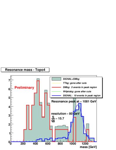
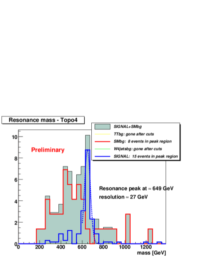
Figure 1: Reconstructed resonances and backgrounds for the ChL model, 1.2 TeV (left) and for the Higgsless model, 700 GeV (right), in the 2-lepton channel. Although no $t\bar{t}$ nor $Wj$ background remains, they cannot be statistically excluded.

3.1 $qqWZ\to qq\ell\nu\ell\ell$

This channel is relatively clean, because of the presence of three leptons, but it is suppressed by the branching ratios. We will therefore consider a signal for an integrated luminosity of 300 fb^-1, for an integrated luminosity of 100 fb^-1.

We apply similar cuts to the case above, with the difference that we require the presence of 3 leptons with $p_{T}>40$ GeV, as well as transverse momentum of $\not{p}_{T}>40$ GeV. The transverse momentum of the neutrino is assumed to be the measured $\not{p}_{T}$ and the longitudinal momentum is constrained by requiring that $m_{\ell\nu}=m_{W}$. We also require that two opposite sign, same flavour leptons have the mass of the $Z$ within 15 GeV. With these cuts, no events remain from $t\bar{t}$ and other backgrounds (except the irreducible SM $qqWZ$ background), although the statistics are insufficient to claim that they are completely eliminated. Figs. 2 shows preliminary results for the ChL and Higgsless models studied here.

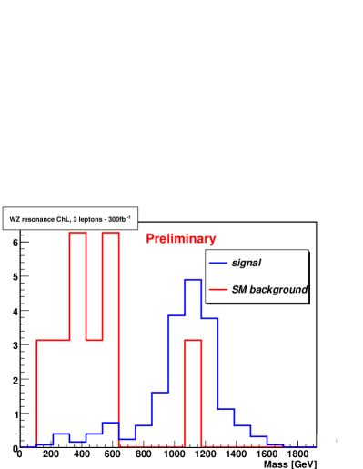
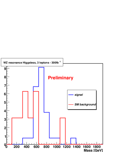
Figure 2: Reconstructed resonances and backgrounds for the ChL model, 1.2 TeV (left) and for the Higgsless model, 700 GeV (right), in the 3-lepton channel, for an integrated luminosity of 300 fb^-1.Although no $t\bar{t}$ nor $Wj$ background remains, they cannot be statistically excluded.

4 CONCLUSION

The reconstruction of high mass $WZ$ resonances arising from a Chiral Lagrangian model and from a Higgsless model have been studied using full detector simulation. Although insufficient statistics were available for background estimation, preliminary results show that, with appropriate cuts, and depending on the parameters of the models, significant signals can be obtained within 1-3 years of data taking at the LHC at nominal luminosity (corresponding to 100-300 fb^-1).

References

- [1] H. Nilles, Phys. Rev. 110 (1984) 1.
- [2] C. L. Bennett et. al., Astrophys. J. Suppl. 148 (2003) 1, [astro-ph/0302207].
- [3] D. N. Spergel et. al.,, WMAP Collaboration Astrophys. J. Suppl. 148 (2003) 175, [astro-ph/0302209].
- [4] J. R. Ellis, K. A. Olive, Y. Santoso, and V. C. Spanos, Phys. Lett. B565 (2003) 176–182, [hep-ph/0303043].
- [5] G. Bélanger, F. Boudjema, A. Pukhov, and A. Semenov, Comput. Phys. Commun. 149 (2002) 103–120, [hep-ph/0112278].
- [6] G. Belanger, F. Boudjema, A. Pukhov, and A. Semenov, hep-ph/0405253.
- [7] F. Paige, S. Protopescu, H. Baer, and X. Tata, hep-ph/0312045.
- [8] H. Baer and C. Balazs, JCAP 0305 (2003) 006, [hep-ph/0303114].
- [9] B. C. Allanach et. al.,, Beyond the Standard Model Working Group Collaboration hep-ph/0402295.
- [10] U. De Sanctis, T. Lari, S. Montesano, and C. Troncon, ATLAS Internal note, in preparation.
- [11] G. Corcella et. al., JHEP 01 (2001) 010, [hep-ph/0011363].
- [12] S. Moretti et. al., JHEP 04 (2002) 028, [hep-ph/0204123].
- [13] G. Corcella et. al., hep-ph/0210213.
- [14] S. Frixione and B. Webber, JHEP 06 (2002) 029, [hep-ph/0204244].
- [15] S. Frixione, P. Nason, and B. Webber, JHEP 08 (2003) 007, [hep-ph/0305252].
- [16] T. Sjöstrand, L. Lonnblad, and S. Mrenna, hep-ph/0108264.
- [17] T. Sjöstrand et. al., Comput. Phys. Commun. 135 (2001) 238–259, [hep-ph/0010017].
- [18] E. Richter-Was, D. Froidevaux, and L. Poggioli, ATL-PHYS-98-131.
- [19] M. Nojiri and Y. Yamada, Phys. Rev. D60 (1999) 015006, [hep-ph/9902201].
- [20] T. Lari, U. Troncon, U. De Sanctis, and S. Montesano,. These proceedings.
- [21] T. Tsukamoto, K. Fujii, H. Murayama, M. Yamaguchi, and Y. Okada, Phys. Rev. D51 (1995) 3153–3171.
- [22] J. L. Feng, M. E. Peskin, H. Murayama, and X. Tata, Phys. Rev. D52 (1995) 1418–1432, [hep-ph/9502260].
- [23] S. Y. Choi, A. Djouadi, H. K. Dreiner, J. Kalinowski, and P. M. Zerwas, Eur. Phys. J. C7 (1999) 123–134, [hep-ph/9806279].
- [24] S. Y. Choi et. al., Eur. Phys. J. C14 (2000) 535–546, [hep-ph/0002033].
- [25] J. L. Kneur and G. Moultaka, Phys. Rev. D61 (2000) 095003, [hep-ph/9907360].
- [26] S. Y. Choi, J. Kalinowski, G. Moortgat-Pick, and P. M. Zerwas, Eur. Phys. J. C22 (2001) 563–579, [hep-ph/0108117].
- [27] S. Y. Choi, J. Kalinowski, G. Moortgat-Pick, and P. M. Zerwas, hep-ph/0202039.
- [28] H. Baer et. al., hep-ph/9503479.
- [29] G. Moortgat-Pick, H. Fraas, A. Bartl, and W. Majerotto, Eur. Phys. J. C7 (1999) 113–122, [hep-ph/9804306].
- [30] G. Moortgat-Pick,.
- [31] G. Moortgat-Pick and H. Fraas, Phys. Rev. D59 (1999) 015016, [hep-ph/9708481].
- [32] G. Moortgat-Pick and H. Fraas, Acta Phys. Polon. B30 (1999) 1999–2011, [hep-ph/9904209].
- [33] G. Moortgat-Pick, A. Bartl, H. Fraas, and W. Majerotto, Eur. Phys. J. C18 (2000) 379–391, [hep-ph/0007222].
- [34] K. Desch, J. Kalinowski, G. Moortgat-Pick, K. Rolbiecki, and J. Stirling, In preparation.
- [35] W. Porod, Comput. Phys. Commun. 153 (2003) 275–315, [hep-ph/0301101].
- [36] W. J. Stirling, Nucl. Phys. B456 (1995) 3–24, [hep-ph/9503320].
- [37] T. Abe et. al.,, American Linear Collider Working Group Collaboration hep-ex/0106056.
- [38] J. A. Aguilar-Saavedra et. al.,, ECFA/DESY LC Physics Working Group Collaboration hep-ph/0106315.
- [39] K. Abe et. al.,, ACFA Linear Collider Working Group Collaboration hep-ph/0109166.
- [40] G. Moortgat-Pick et. al., hep-ph/0507011.
- [41] H.-C. Cheng, K. T. Matchev, and M. Schmaltz, Phys. Rev. D66 (2002) 056006, [hep-ph/0205314].
- [42] A. J. Barr, Phys. Lett. B596 (2004) 205–212, [hep-ph/0405052].
- [43] J. M. Smillie and B. R. Webber, JHEP 10 (2005) 069, [hep-ph/0507170].
- [44] A. Datta, K. Kong, and K. T. Matchev, Phys. Rev. D72 (2005) 096006, [hep-ph/0509246].
- [45] B. C. Allanach et. al., Eur. Phys. J. C25 (2002) 113–123, [hep-ph/0202233].
- [46] T. Sjostrand, L. Lonnblad, S. Mrenna, and P. Skands, hep-ph/0308153.
- [47] H. L. Lai et. al., Eur. Phys. J. C12 (2000) 375–392, [hep-ph/9903282].
- [48] S. Eidelman et. al.,, Particle Data Group Collaboration Phys. Lett. B592 (2004) 1.
- [49] A. Strong, I. Moskalenko, and O. Reimer, Astrophys. J. 613 (2004) 962–976, [astro-ph/0406254].
- [50] W. de Boer et. al., astro-ph/0408272.
- [51] G. Bertone, D. Hooper, and J. Silk, Phys. Rept. 405 (2005) 279–390, [hep-ph/0404175].
- [52] A. Collaboration,.
- [53] P. Bechtle, K. Desch, W. Porod, and P. Wienemann, hep-ph/0511006.
- [54] P. Bechtle, K. Desch, and P. Wienemann, hep-ph/0412012.
- [55] R. Lafaye, T. Plehn, and D. Zerwas, hep-ph/0512028.
- [56] R. Lafaye, T. Plehn, and D. Zerwas, hep-ph/0404282.
- [57] M. Drees and S. P. Martin, hep-ph/9504324.
- [58] J. L. Feng, K. T. Matchev, and T. Moroi, Phys. Rev. Lett. 84 (2000) 2322–2325, [hep-ph/9908309].
- [59] J. L. Feng, K. T. Matchev, and F. Wilczek, Phys. Lett. B482 (2000) 388–399, [hep-ph/0004043].
- [60] A. Datta, A. Djouadi, M. Guchait, and F. Moortgat, Nucl. Phys. B681 (2004) 31–64, [hep-ph/0303095].
- [61] E. L. Berger, T. Han, J. Jiang, and T. Plehn, Phys. Rev. D71 (2005) 115012, [hep-ph/0312286].
- [62] A. Djouadi, J.-L. Kneur, and G. Moultaka, hep-ph/0211331.
- [63] V. D. Barger and C. Kao, Phys. Rev. D60 (1999) 115015, [hep-ph/9811489].
- [64] K. T. Matchev and D. M. Pierce, Phys. Rev. D60 (1999) 075004, [hep-ph/9904282].
- [65] K. T. Matchev and D. M. Pierce, Phys. Lett. B467 (1999) 225–231, [hep-ph/9907505].
- [66] H. Baer, M. Drees, F. Paige, P. Quintana, and X. Tata, Phys. Rev. D61 (2000) 095007, [hep-ph/9906233].
- [67] S. Abel et. al.,, SUGRA Working Group Collaboration hep-ph/0003154.
- [68] W. Beenakker et. al., Phys. Rev. Lett. 83 (1999) 3780–3783, [hep-ph/9906298].
- [69] V. Shiltsev,.
- [70] H. Baer, C.-h. Chen, F. Paige, and X. Tata, Phys. Rev. D50 (1994) 4508–4516, [hep-ph/9404212].
- [71] D. Denegri, W. Majerotto, and L. Rurua, Phys. Rev. D58 (1998) 095010, [hep-ph/9711357].
- [72] H. Baer, C.-h. Chen, M. Drees, F. Paige, and X. Tata, Phys. Rev. D59 (1999) 055014, [hep-ph/9809223].
- [73] H. Baer, T. Krupovnickas, S. Profumo, and P. Ullio, JHEP 10 (2005) 020, [hep-ph/0507282].
- [74] T. Hahn, W. Hollik, S. Heinemeyer, and G. Weiglein, hep-ph/0507009.
- [75] G. Weiglein et. al.,, LHC/LC Study Group Collaboration hep-ph/0410364.
- [76] W. de Boer, M. Herold, C. Sander, and V. Zhukov, Eur. Phys. J. C33 (2004) s981–s983, [hep-ph/0312037].
- [77] W. de Boer, C. Sander, V. Zhukov, A. Gladyshev, and D. Kazakov, astro-ph/0508617.
- [78] V. Berezinsky, V. Dokuchaev, and Y. Eroshenko, astro-ph/0511494.
- [79] A. Strong and I. Moskalenko, astro-ph/9812260.
- [80] W. de Boer and C. Sander, Phys. Lett. B585 (2004) 276–286, [hep-ph/0307049].
- [81] H. V. Peiris et. al., Astrophys. J. Suppl. 148 (2003) 213, [astro-ph/0302225].
- [82] G. Belanger, F. Boudjema, A. Pukhov, and A. Semenov, hep-ph/0210327.
- [83] G. Belanger, S. Kraml, and A. Pukhov, Phys. Rev. D72 (2005) 015003, [hep-ph/0502079].
- [84] U. Chattopadhyay, A. Corsetti, and P. Nath, Phys. Rev. D68 (2003) 035005, [hep-ph/0303201].
- [85] S. Profumo and C. E. Yaguna, Phys. Rev. D70 (2004) 095004, [hep-ph/0407036].
- [86] E. A. Baltz and P. Gondolo, JHEP 10 (2004) 052, [hep-ph/0407039].
- [87] G. Belanger, F. Boudjema, A. Cottrant, A. Pukhov, and A. Semenov, Nucl. Phys. B706 (2005) 411–454, [hep-ph/0407218].
- [88] A. B. Lahanas and D. V. Nanopoulos, Phys. Lett. B568 (2003) 55–62, [hep-ph/0303130].
- [89] T. Nihei and M. Sasagawa, Phys. Rev. D70 (2004) 055011, [hep-ph/0404100].
- [90] M. E. Gomez, T. Ibrahim, P. Nath, and S. Skadhauge, Phys. Rev. D72 (2005) 095008, [hep-ph/0506243].
- [91] C. Balazs, M. Carena, A. Menon, D. E. Morrissey, and C. E. M. Wagner, Phys. Rev. D71 (2005) 075002, [hep-ph/0412264].
- [92] P. Skands et. al., JHEP 07 (2004) 036, [hep-ph/0311123].
- [93] S. Y. Choi, M. Drees, J. S. Lee, and J. Song, Eur. Phys. J. C25 (2002) 307–313, [hep-ph/0204200].
- [94] G. Belanger, F. Boudjema, A. Pukhov, and A. Semenov,. These proceedings.
- [95] A. V. Semenov, hep-ph/0208011.
- [96] A. Pukhov, hep-ph/0412191.
- [97] J. S. Lee et. al., Comput. Phys. Commun. 156 (2004) 283–317, [hep-ph/0307377].
- [98] B. C. Allanach, G. Belanger, F. Boudjema, and A. Pukhov, JHEP 12 (2004) 020, [hep-ph/0410091].
- [99] P. Gondolo and K. Freese, JHEP 07 (2002) 052, [hep-ph/9908390].
- [100] A. D. Sakharov, Pisma Zh. Eksp. Teor. Fiz. 5 (1967) 32–35.
- [101] J. M. Carmona, J. L. Cortes, A. Das, J. Gamboa, and F. Mendez, hep-th/0410143.
- [102] A. G. Cohen, D. B. Kaplan, and A. E. Nelson, Ann. Rev. Nucl. Part. Sci. 43 (1993) 27–70, [hep-ph/9302210].
- [103] M. Quiros, Helv. Phys. Acta 67 (1994) 451–583.
- [104] V. A. Rubakov and M. E. Shaposhnikov, Usp. Fiz. Nauk 166 (1996) 493–537, [hep-ph/9603208].
- [105] A. Riotto and M. Trodden, Ann. Rev. Nucl. Part. Sci. 49 (1999) 35–75, [hep-ph/9901362].
- [106] M. Quiros and M. Seco, Nucl. Phys. Proc. Suppl. 81 (2000) 63–70, [hep-ph/9903274].
- [107] G. ’t Hooft, Phys. Rev. D14 (1976) 3432–3450.
- [108] N. S. Manton, Phys. Rev. D28 (1983) 2019.
- [109] F. R. Klinkhamer and N. S. Manton, Phys. Rev. D30 (1984) 2212.
- [110] D. Bodeker, Phys. Lett. B426 (1998) 351–360, [hep-ph/9801430].
- [111] P. Arnold and L. G. Yaffe, Phys. Rev. D62 (2000) 125014, [hep-ph/9912306].
- [112] P. Arnold, Phys. Rev. D62 (2000) 036003, [hep-ph/9912307].
- [113] G. D. Moore and K. Rummukainen, Phys. Rev. D61 (2000) 105008, [hep-ph/9906259].
- [114] G. D. Moore, Phys. Rev. D62 (2000) 085011, [hep-ph/0001216].
- [115] A. G. Cohen, D. B. Kaplan, and A. E. Nelson, Phys. Lett. B336 (1994) 41–47, [hep-ph/9406345].
- [116] P. Huet and A. E. Nelson, Phys. Rev. D53 (1996) 4578–4597, [hep-ph/9506477].
- [117] A. I. Bochkarev and M. E. Shaposhnikov, Mod. Phys. Lett. A2 (1987) 417.
- [118] K. Jansen, Nucl. Phys. Proc. Suppl. 47 (1996) 196–211, [hep-lat/9509018].
- [119] K. Rummukainen, M. Tsypin, K. Kajantie, M. Laine, and M. E. Shaposhnikov, Nucl. Phys. B532 (1998) 283–314, [hep-lat/9805013].
- [120] K. Rummukainen, K. Kajantie, M. Laine, M. E. Shaposhnikov, and M. Tsypin, hep-ph/9809435.
- [121] M. Carena, M. Quiros, and C. E. M. Wagner, Phys. Lett. B380 (1996) 81–91, [hep-ph/9603420].
- [122] M. Laine, Nucl. Phys. B481 (1996) 43–84, [hep-ph/9605283].
- [123] M. Losada, Phys. Rev. D56 (1997) 2893–2913, [hep-ph/9605266].
- [124] G. R. Farrar and M. Losada, Phys. Lett. B406 (1997) 60–65, [hep-ph/9612346].
- [125] B. de Carlos and J. R. Espinosa, Nucl. Phys. B503 (1997) 24–54, [hep-ph/9703212].
- [126] D. Bodeker, P. John, M. Laine, and M. G. Schmidt, Nucl. Phys. B497 (1997) 387–414, [hep-ph/9612364].
- [127] M. Carena, M. Quiros, and C. E. M. Wagner, Nucl. Phys. B524 (1998) 3–22, [hep-ph/9710401].
- [128] M. Laine and K. Rummukainen, Nucl. Phys. B535 (1998) 423–457, [hep-lat/9804019].
- [129] M. Losada, Nucl. Phys. B537 (1999) 3–31, [hep-ph/9806519].
- [130] M. Losada, Nucl. Phys. B569 (2000) 125–157, [hep-ph/9905441].
- [131] M. Laine and M. Losada, Nucl. Phys. B582 (2000) 277–295, [hep-ph/0003111].
- [132] M. Laine and K. Rummukainen, Nucl. Phys. B597 (2001) 23–69, [hep-lat/0009025].
- [133] R. Barate et. al.,, LEP Working Group for Higgs boson searches Collaboration Phys. Lett. B565 (2003) 61–75, [hep-ex/0306033].
- [134] J. R. Ellis, G. Ridolfi, and F. Zwirner, Phys. Lett. B257 (1991) 83–91.
- [135] Y. Okada, M. Yamaguchi, and T. Yanagida, Prog. Theor. Phys. 85 (1991) 1–6.
- [136] H. E. Haber and R. Hempfling, Phys. Rev. Lett. 66 (1991) 1815–1818.
- [137] M. Carena, M. Quiros, A. Riotto, I. Vilja, and C. E. M. Wagner, Nucl. Phys. B503 (1997) 387–404, [hep-ph/9702409].
- [138] J. M. Cline, M. Joyce, and K. Kainulainen, JHEP 07 (2000) 018, [hep-ph/0006119].
- [139] M. Carena, J. M. Moreno, M. Quiros, M. Seco, and C. E. M. Wagner, Nucl. Phys. B599 (2001) 158–184, [hep-ph/0011055].
- [140] M. Carena, M. Quiros, M. Seco, and C. E. M. Wagner, Nucl. Phys. B650 (2003) 24–42, [hep-ph/0208043].
- [141] D. Chang, W.-F. Chang, and W.-Y. Keung, Phys. Rev. D66 (2002) 116008, [hep-ph/0205084].
- [142] A. Pilaftsis, Nucl. Phys. B644 (2002) 263–289, [hep-ph/0207277].
- [143] M. Tegmark et. al.,, SDSS Collaboration Phys. Rev. D69 (2004) 103501, [astro-ph/0310723].
- [144] R. Arnowitt, B. Dutta, B. Hu, and Y. Santoso, Phys. Lett. B505 (2001) 177–183, [hep-ph/0102344].
- [145] A. Djouadi, M. Drees, and J. L. Kneur, JHEP 08 (2001) 055, [hep-ph/0107316].
- [146] J. R. Ellis, K. A. Olive, Y. Santoso, and V. C. Spanos, Phys. Lett. B588 (2004) 7–16, [hep-ph/0312262].
- [147] J. R. Ellis, K. A. Olive, Y. Santoso, and V. C. Spanos, Phys. Rev. D69 (2004) 095004, [hep-ph/0310356].
- [148] A. B. Lahanas, N. E. Mavromatos, and D. V. Nanopoulos, Int. J. Mod. Phys. D12 (2003) 1529–1591, [hep-ph/0308251].
- [149] J. L. Feng, S. Su, and F. Takayama, Phys. Rev. D70 (2004) 075019, [hep-ph/0404231].
- [150] J. L. Feng, S.-f. Su, and F. Takayama, Phys. Rev. D70 (2004) 063514, [hep-ph/0404198].
- [151] J. R. Ellis, A. Ferstl, and K. A. Olive, Phys. Rev. D63 (2001) 065016, [hep-ph/0007113].
- [152] D. S. Akerib et. al.,, CDMS Collaboration astro-ph/0509259.
- [153] D. B. Cline, H.-g. Wang, and Y. Seo, eConf C010630 (2001) E108, [astro-ph/0108147].
- [154] R. J. Gaitskell,, XENON Collaboration. Prepared for IDM 2004: 5th International Workshop on the Identification of Dark Matter, Edinburgh, Scotland, United Kingdom, 6-10 Sep 2004.
- [155] S. Heinemeyer, W. Hollik, and G. Weiglein, Eur. Phys. J. C9 (1999) 343–366, [hep-ph/9812472].
- [156] G. Degrassi, S. Heinemeyer, W. Hollik, P. Slavich, and G. Weiglein, Eur. Phys. J. C28 (2003) 133–143, [hep-ph/0212020].
- [157] M. Carena, A. Finch, A. Freitas, C. Milsténe, H. Nowak, and A. Sopczak, Phys. Rev. D72 (2005) 115008, [hep-ph/0508152].
- [158] D. Delepine, J. M. Gerard, R. Gonzalez Felipe, and J. Weyers, Phys. Lett. B386 (1996) 183–188, [hep-ph/9604440].
- [159] J. M. Cline and G. D. Moore, Phys. Rev. Lett. 81 (1998) 3315–3318, [hep-ph/9806354].
- [160] C. Balazs, M. Carena, and C. E. M. Wagner, Phys. Rev. D70 (2004) 015007, [hep-ph/0403224].
- [161] S. Kraml and A. R. Raklev, hep-ph/0512284.
- [162] W. Beenakker, R. Hopker, and M. Spira, hep-ph/9611232. See http://pheno.physics.wisc.edu/plehn/.
- [163] E. Richter-Was, hep-ph/0207355.
- [164] ATLAS Collaboration CERN-LHCC-97-16.
- [165] T. Stelzer and W. F. Long, Comput. Phys. Commun. 81 (1994) 357–371, [hep-ph/9401258].
- [166] F. Maltoni and T. Stelzer, JHEP 02 (2002) 044.
- [167] I. Hinchliffe, F. E. Paige, M. D. Shapiro, J. Soderqvist, and W. Yao, Phys. Rev. D55 (1997) 5520–5540, [hep-ph/9610544].
- [168] H. Bachacou, I. Hinchliffe, and F. E. Paige, Phys. Rev. D62 (2000) 015009, [hep-ph/9907518].
- [169] B. C. Allanach, C. G. Lester, M. A. Parker, and B. R. Webber, JHEP 09 (2000) 004, [hep-ph/0007009].
- [170] C. G. Lester, CERN-THESIS-2004-003.
- [171] D. J. Gjelsten, B. K. Miller and P. Osland, JHEP 12 (2004) 003, [hep-ph/0410303].
- [172] D. J. Miller, P. Osland, and A. R. Raklev, hep-ph/0510356.
- [173] W. Beenakker, M. Kramer, T. Plehn, M. Spira, and P. M. Zerwas, Nucl. Phys. B515 (1998) 3–14, [hep-ph/9710451].
- [174] ATLAS Collaboration CERN/LHCC 99-14/15 (1999).
- [175] T. Sjöstrand, Comput. Phys. Commun. 82 (1994) 74–90.
- [176] M. L. Mangano, M. Moretti, F. Piccinini, R. Pittau, and A. D. Polosa, JHEP 07 (2003) 001, [hep-ph/0206293].
- [177] A. Djouadi et. al., hep-ph/0002258.
- [178] B. Kileng, Z. Phys. C63 (1994) 87–98, [hep-ph/9303293].
- [179] B. Kileng, P. Osland, and P. N. Pandita, Z. Phys. C71 (1996) 87–94, [hep-ph/9506455].
- [180] G. L. Kane, G. D. Kribs, S. P. Martin, and J. D. Wells, Phys. Rev. D53 (1996) 213–220, [hep-ph/9508265].
- [181] A. Djouadi, Phys. Lett. B435 (1998) 101–108, [hep-ph/9806315].
- [182] A. Djouadi, Mod. Phys. Lett. A14 (1999) 359–368, [hep-ph/9903382].
- [183] G. Belanger, F. Boudjema, and K. Sridhar, Nucl. Phys. B568 (2000) 3–39, [hep-ph/9904348].
- [184] A. Djouadi, J. L. Kneur, and G. Moultaka, Phys. Rev. Lett. 80 (1998) 1830–1833, [hep-ph/9711244].
- [185] A. Djouadi, J. L. Kneur, and G. Moultaka, Nucl. Phys. B569 (2000) 53–81, [hep-ph/9903218].
- [186] A. Dedes and S. Moretti, Phys. Rev. D60 (1999) 015007, [hep-ph/9812328].
- [187] A. Dedes and S. Moretti, Eur. Phys. J. C10 (1999) 515–535, [hep-ph/9904491].
- [188] A. Dedes and S. Moretti, hep-ph/9909526.
- [189] http://www.hep.phy.cam.ac.uk/richardn/HERWIG/ISAWIG/, and links therein.
- [190] A. Sopczak, Talk ’Scalar Top Quark Studies with Small Visible Energy’, SUSY’05 Conference, Durham, UK.
- [191] C. Milstene and A. Sopczak, contribution to Snowmass LCWS 2005 workshop, ‘LCFI Vertex Detector Design Studies’, Aug. 14-27, 2005.
- [192] A. Finch, H. Nowak, A. Sopczak, “Determination of the Scalar Top Mass at a Linear Collider”, in Proc. of the International Conference on Linear Colliders (LCWS 04), Paris, France, 19-24 April 2004.
- [193] J. Malmgren and K. Johansson, Nucl. Inst. Methods A 403 (1998) 481.
- [194] A. Finch, H. Nowak, A. Sopczak, contributed paper EPS370, Int. Conference on High-Energy Physics (HEP 2003), Aachen, Germany, 17-23 July 2003 [LC Note LC-PHSM-2003-075].
- [195] A. Bartl, H. Eberl, S. Kraml, W. Majerotto, W. Porod, and A. Sopczak, Z. Phys. C76 (1997) 549–560, [hep-ph/9701336].
- [196] J. L. Feng and D. E. Finnell, Phys. Rev. D49 (1994) 2369–2381, [hep-ph/9310211].
- [197] A. Sopczak, in PHYSICS AT LEP2, “Event Generators for Discovery Physics”, CERN Yellow Report CERN 96-01.
- [198] M. Pohl and H. J. Schreiber, hep-ex/0206009.
- [199] LEP2 SUSY Working Group, ALEPH, DELPHI, L3 and OPAL experiments, note LEPSUSYWG/04-02.1.
- [200] R. Demina, J. D. Lykken, K. T. Matchev, and A. Nomerotski, Phys. Rev. D62 (2000) 035011, [hep-ph/9910275].
- [201] F. Franke and H. Fraas, Z. Phys. C72 (1996) 309–325, [hep-ph/9511275].
- [202] F. Franke and H. Fraas, Int. J. Mod. Phys. A12 (1997) 479–534, [hep-ph/9512366].
- [203] F. Franke, H. Fraas, and A. Bartl, Phys. Lett. B336 (1994) 415–422, [hep-ph/9408217].
- [204] S. Y. Choi, D. J. Miller, and P. M. Zerwas, Nucl. Phys. B711 (2005) 83–111, [hep-ph/0407209].
- [205] U. Ellwanger and C. Hugonie, Eur. Phys. J. C13 (2000) 681–690, [hep-ph/9812427].
- [206] S. Hesselbach, F. Franke, and H. Fraas, Phys. Lett. B492 (2000) 140–147, [hep-ph/0007310].
- [207] F. Franke and S. Hesselbach, Phys. Lett. B526 (2002) 370–378, [hep-ph/0111285].
- [208] S. Hesselbach and F. Franke, hep-ph/0210363.
- [209] G. Moortgat-Pick, S. Hesselbach, F. Franke, and H. Fraas, hep-ph/9909549.
- [210] S. Hesselbach, F. Franke, and H. Fraas, hep-ph/0003272.
- [211] S. Hesselbach, F. Franke, and H. Fraas, Eur. Phys. J. C23 (2002) 149–162, [hep-ph/0107080].
- [212] G. Moortgat-Pick, S. Hesselbach, F. Franke, and H. Fraas, JHEP 06 (2005) 048, [hep-ph/0502036].
- [213] G. Moortgat-Pick, S. Hesselbach, F. Franke, and H. Fraas, hep-ph/0508313.
- [214] G. Polesello, J. Phys. G30 (2004) 1185–1199.
- [215] K. Desch, J. Kalinowski, G. Moortgat-Pick, M. M. Nojiri, and G. Polesello, JHEP 02 (2004) 035, [hep-ph/0312069].
- [216] U. Ellwanger and C. Hugonie, Eur. Phys. J. C25 (2002) 297–305, [hep-ph/9909260].
- [217] D. J. Miller, R. Nevzorov, and P. M. Zerwas, Nucl. Phys. B681 (2004) 3–30, [hep-ph/0304049].
- [218] U. Ellwanger, J. F. Gunion, and C. Hugonie, JHEP 02 (2005) 066, [hep-ph/0406215].
- [219] U. Ellwanger, J. F. Gunion, and C. Hugonie, JHEP 07 (2005) 041, [hep-ph/0503203].
- [220] P. Bechtle, K. Desch, and P. Wienemann, hep-ph/0506244.
- [221] P. Bechtle, K. Desch, F. Franke, S. Hesselbach, G. Moortgat-Pick, W. Porod, and P. Wienemann, in progress.
- [222] N. Arkani-Hamed and S. Dimopoulos, JHEP 06 (2005) 073, [hep-th/0405159].
- [223] G. F. Giudice and A. Romanino, Nucl. Phys. B699 (2004) 65–89, [hep-ph/0406088].
- [224] N. Arkani-Hamed, S. Dimopoulos, G. F. Giudice, and A. Romanino, Nucl. Phys. B709 (2005) 3–46, [hep-ph/0409232].
- [225] A. Dobado, M. J. Herrero, and S. Peñaranda, Eur. Phys. J. C7 (1999) 313–339, [hep-ph/9710313].
- [226] A. Dobado, M. J. Herrero, and S. Peñaranda, Eur. Phys. J. C17 (2000) 487–500, [hep-ph/0002134].
- [227] S. Dimopoulos,. Splitting SUSY, talk at the 13th Int. Conf. on Supersymmetry and the Unification of Fundamental Interactions, 18–23 July, 2005, IPPP Durham, UK, http://susy-2005.dur.ac.uk/PLENARY/THU/dimopoulos SUSY2005copy.ppt, and references therein.
- [228] J. Guasch and S. Peñaranda, JHEP 01 (2006) 121, [hep-ph/0508241].
- [229] S. P. Martin, K. Tobe, and J. D. Wells, Phys. Rev. D71 (2005) 073014, [hep-ph/0412424].
- [230] M. E. Peskin and T. Takeuchi, Phys. Rev. D46 (1992) 381–409.
- [231] I. Maksymyk, C. P. Burgess, and D. London, Phys. Rev. D50 (1994) 529–535, [hep-ph/9306267].
- [232] R. Barbieri, A. Pomarol, R. Rattazzi, and A. Strumia, Nucl. Phys. B703 (2004) 127–146, [hep-ph/0405040].
- [233] G. Marandella, C. Schappacher, and A. Strumia, Nucl. Phys. B715 (2005) 173–189, [hep-ph/0502095].
- [234] D. Y. Bardin et. al., hep-ph/9412201.
- [235] D. Y. Bardin et. al., Comput. Phys. Commun. 133 (2001) 229–395, [hep-ph/9908433].
- [236] J. A. Grifols and J. Solà, Nucl. Phys. B253 (1985) 47.
- [237] D. Garcia and J. Solà, Mod. Phys. Lett. A9 (1994) 211–224.
- [238] D. Garcia, R. A. Jiménez, and J. Solà, Phys. Lett. B347 (1995) 309–320, [hep-ph/9410310].
- [239] D. Garcia, R. A. Jiménez, and J. Solà, Phys. Lett. B347 (1995) 321–331, [hep-ph/9410311].
- [240] J. Kublbeck, M. Bohm, and A. Denner, Comput. Phys. Commun. 60 (1990) 165–180.
- [241] T. Hahn, Comput. Phys. Commun. 140 (2001) 418–431, [hep-ph/0012260].
- [242] T. Hahn and C. Schappacher, Comput. Phys. Commun. 143 (2002) 54–68, [hep-ph/0105349].
- [243] T. Hahn and M. Perez-Victoria, Comput. Phys. Commun. 118 (1999) 153–165, [hep-ph/9807565].
- [244] G. J. van Oldenborgh and J. A. M. Vermaseren, Z. Phys. C46 (1990) 425–438.
- [245] T. Hahn,. FeynArts, FormCalc and LoopTools user’s guides, available from http://www.feynarts.de.
- [246] A. Yamada, Z. Phys. C61 (1994) 247–263.
- [247] P. Chankowski, S. Pokorski, and J. Rosiek, Nucl. Phys. B423 (1994) 437–496, [hep-ph/9303309].
- [248] A. Dabelstein, Z. Phys. C67 (1995) 495–512, [hep-ph/9409375].
- [249] A. Dabelstein, Nucl. Phys. B456 (1995) 25–56, [hep-ph/9503443].
- [250] G. Altarelli and M. W. Grunewald, Phys. Rept. 403-404 (2004) 189–201, [hep-ph/0404165].
- [251] CDF Collaboration hep-ex/0507091.
- [252] A. Arvanitaki, C. Davis, P. W. Graham, A. Pierce, and J. G. Wacker, hep-ph/0504210.
- [253] U. Baur et. al., eConf C010630 (2001) P122, [hep-ph/0111314].
- [254] S. Heinemeyer, S. Kraml, W. Porod, and G. Weiglein, JHEP 09 (2003) 075, [hep-ph/0306181].
- [255] S. Heinemeyer and G. Weiglein, hep-ph/0012364.
- [256] S. Heinemeyer and G. Weiglein, hep-ph/0307177.
- [257] S. Heinemeyer, W. Hollik, and G. Weiglein, hep-ph/0412214.
- [258] LEP Collaboration hep-ex/0312023.
- [259] M. W. Grunewald, hep-ex/0304023.
- [260] S. Haywood et. al., hep-ph/0003275.
- [261] R. Hawkings and K. Monig, Eur. Phys. J. direct C1 (1999) 8, [hep-ex/9910022].
- [262] S. Heinemeyer, T. Mannel, and G. Weiglein, hep-ph/9909538.
- [263] J. Erler, S. Heinemeyer, W. Hollik, G. Weiglein, and P. M. Zerwas, Phys. Lett. B486 (2000) 125–133, [hep-ph/0005024].
- [264] J. Erler and S. Heinemeyer, hep-ph/0102083.
- [265] I. Antoniadis and S. Dimopoulos, Nucl. Phys. B715 (2005) 120–140, [hep-th/0411032].
- [266] I. Antoniadis, A. Delgado, K. Benakli, M. Quiros, and M. Tuckmantel, hep-ph/0507192.
- [267] A. Font and L. E. Ibanez, JHEP 03 (2005) 040, [hep-th/0412150].
- [268] P. J. Fox, A. E. Nelson, and N. Weiner, JHEP 08 (2002) 035, [hep-ph/0206096].
- [269] I. Antoniadis, K. Benakli, A. Delgado, M. Quiros, and M. Tuckmantel, hep-th/0601003.
- [270] I. Antoniadis, K. S. Narain, and T. R. Taylor, Nucl. Phys. B729 (2005) 235–277, [hep-th/0507244].
- [271] N. Arkani-Hamed, S. Dimopoulos, and S. Kachru, hep-th/0501082.
- [272] C. H. Chen, M. Drees, and J. F. Gunion, Phys. Rev. Lett. 76 (1996) 2002–2005, [hep-ph/9512230].
- [273] M. R. Whalley, D. Bourilkov, and R. C. Group, hep-ph/0508110.
- [274] S. Jadach, J. H. Kuhn, and Z. Was, Comput. Phys. Commun. 64 (1990) 275–299.
- [275] ATLAS, ATLAS TDR-016.
- [276] S. Y. Choi, J. Kalinowski, Y. Liao, and P. M. Zerwas, Eur. Phys. J. C40 (2005) 555–564, [hep-ph/0407347].
- [277] S. Heinemeyer, Eur. Phys. J. C22 (2001) 521–534, [hep-ph/0108059].
- [278] R. M. Godbole et. al., hep-ph/0404024.
- [279] ATLAS Collaboration Detector and Physics Performance Technical Design Report, CERN-LHCC-99-14 & 15 (1999).
- [280] CMS Collaboration Technical Design Report, CERN-LHCC-97-10 (1997).
- [281] M. Hohlfeld, ATLAS Report, ATL-PHYS-2001-004 (2001).
- [282] S. Y. Choi, D. J. Miller, M. M. Muhlleitner, and P. M. Zerwas, Phys. Lett. B553 (2003) 61–71, [hep-ph/0210077].
- [283] M. Spira, hep-ph/9510347.
- [284] A. Collaboration, CERN-LHCC-99-15.
- [285] G. A. Blair, W. Porod, and P. M. Zerwas, Phys. Rev. D63 (2001) 017703, [hep-ph/0007107].
- [286] M. A. Dobbs et. al., hep-ph/0403045. In Les Houches ’Physics at Tev Colliders 2003’ QCD/SM Working Group: Summary Report.
- [287] P. Z. Skands, hep-ph/0507129.
- [288] S. Heinemeyer et. al., hep-ph/0511332.
- [289] J. Reuter et. al., hep-ph/0512012.
- [290] C. M. Harris, P. Richardson, and B. R. Webber, JHEP 08 (2003) 033, [hep-ph/0307305].
- [291] A. Pilaftsis, Phys. Rev. D58 (1998) 096010, [hep-ph/9803297].
- [292] A. Pilaftsis, Phys. Lett. B435 (1998) 88–100, [hep-ph/9805373].
- [293] S. Y. Choi and J. S. Lee, Phys. Rev. D61 (2000) 015003, [hep-ph/9907496].
- [294] S. Y. Choi, K. Hagiwara, and J. S. Lee, Phys. Rev. D64 (2001) 032004, [hep-ph/0103294].
- [295] A. Pilaftsis and C. E. M. Wagner, Nucl. Phys. B553 (1999) 3–42, [hep-ph/9902371].
- [296] D. A. Demir, Phys. Rev. D60 (1999) 055006, [hep-ph/9901389].
- [297] S. Y. Choi, M. Drees, and J. S. Lee, Phys. Lett. B481 (2000) 57–66, [hep-ph/0002287].
- [298] M. Carena, J. R. Ellis, A. Pilaftsis, and C. E. M. Wagner, Nucl. Phys. B586 (2000) 92–140, [hep-ph/0003180].
- [299] M. Carena, J. R. Ellis, A. Pilaftsis, and C. E. M. Wagner, Nucl. Phys. B625 (2002) 345–371, [hep-ph/0111245].
- [300] S. Heinemeyer, W. Hollik, and G. Weiglein, Comput. Phys. Commun. 124 (2000) 76–89, [hep-ph/9812320].
- [301] A. Djouadi, J. Kalinowski, and M. Spira, Comput. Phys. Commun. 108 (1998) 56–74, [hep-ph/9704448].
- [302] H. K. Dreiner, P. Richardson, and M. H. Seymour, JHEP 04 (2000) 008, [hep-ph/9912407].
- [303] A. Freitas, A. von Manteuffel, and P. M. Zerwas, Eur. Phys. J. C34 (2004) 487–512, [hep-ph/0310182].
- [304] A. Freitas, A. von Manteuffel, and P. M. Zerwas, Eur. Phys. J. C40 (2005) 435–445, [hep-ph/0408341].
- [305] U. Ellwanger and C. Hugonie, hep-ph/0508022.
- [306] M. Moretti, T. Ohl, and J. Reuter, hep-ph/0102195.
- [307] J. Bijnens, P. Eerola, M. Maul, A. Mansson, and T. Sjöstrand, Phys. Lett. B503 (2001) 341–348, [hep-ph/0101316].
- [308] K. Lane and S. Mrenna, Phys. Rev. D67 (2003) 115011, [hep-ph/0210299].
- [309] K. R. Lynch, E. H. Simmons, M. Narain, and S. Mrenna, Phys. Rev. D63 (2001) 035006, [hep-ph/0007286].
- [310] A. C. Kraan, J. B. Hansen, and P. Nevski, hep-ex/0511014.
- [311] P. Z. Skands, Eur. Phys. J. C23 (2002) 173–184, [hep-ph/0110137].
- [312] T. Sjöstrand and P. Z. Skands, Nucl. Phys. B659 (2003) 243, [hep-ph/0212264].
- [313] A. Pukhov and P. Skands,, “Les Houches squared event generator for the NMSSM.” FERMILAB-CONF-05-520-T. These proceedings, 2006.
- [314] T. Appelquist, H.-C. Cheng, and B. A. Dobrescu, Phys. Rev. D64 (2001) 035002, [hep-ph/0012100].
- [315] C. Macesanu, C. D. McMullen, and S. Nandi, Phys. Lett. B546 (2002) 253–260, [hep-ph/0207269].
- [316] T. Gleisberg et. al., JHEP 02 (2004) 056, [hep-ph/0311263].
- [317] K. Hagiwara et. al., hep-ph/0512260.
- [318] T. Gleisberg et. al., JHEP 09 (2003) 001, [hep-ph/0306182].
- [319] B. C. Allanach, Comput. Phys. Commun. 143 (2002) 305–331.
- [320] J. F. Gunion and H. E. Haber, Nucl. Phys. B272 (1986) 1. [Erratum-ibid. B402, 567 (1993)].
- [321] P. Z. Skands, hep-ph/0601103. To appear in the TeV4LHC workshop Physics Landscapes summary report.
-
[322]
P. Skands et. al.,, “A repository for beyond-the-standard-model tools.”
FERMILAB-CONF-05-521-T. These proceedings. See also: