Some Features of the Glasma

Abstract

We discuss high energy hadronic collisions within the theory of the Color Glass Condensate. We point out that the initial electric and magnetic fields produced in such collisions are longitudinal. This leads to a novel string like description of the collisions, and a large Chern-Simons charge density made immediately after the collision. The presence of the longitudinal magnetic field suggests that essential to the description of these collisions is the decay of Chern-Simons charge.

BNL–NT–06/10
hep-ph/0602189

, ,

1 Introduction

High energy hadronic collisions can be described as collisions of sheets of Colored Glass Condensate [1, 2, 3, 4, 5, 6, 7, 8, 9]. The degrees of freedom of the Color Glass Condensate are those of high energy density gluonic fields [10, 11, 12, 13, 14, 15, 16]. Because the physical density of gluons becomes large, the typical separation between gluons is small, and therefore $\alpha_{\mathrm{s}}$ is small. The highly coherent gluons fill the phase space up to the maximal occupation number $\sim 1/\alpha_{\mathrm{s}}$ and can thus be thought of as condensed. Because of their high speed and Lorentz time dilation, the valence degrees of freedom are seen by the low $x$ fields as slowly evolving in lightcone time. Systems which evolve over long time scales compared to natural ones are glasses. Hence the name Color Glass Condensate. It is possible to describe this system from first principles in QCD because the coupling is weak.

The equations which describe the color fields in a high energy hadronic collision have been written down in Refs. [1, 2, 3, 4]. For the case where the rapidity dependence of the fields can be ignored, the equations were numerically solved [5, 6, 7, 8, 9]. A successful phenomenology has been applied to RHIC energy collisions of nuclei and dA collisions [17, 18, 19, 20, 21, 22, 23, 24, 25, 26, 27]. Since then, a literature has developed relating this description to issues such as topological charge generation [28, 29, 30, 31] and plasma instabilities [32, 33, 34, 35, 36, 37].

Topological charge generation is related to a number of non-perturbative phenomena in field theory. In electroweak theory, it leads to the anomalous generation of baryon plus lepton number. In QCD, it is related to the violation of U(1) chiral symmetry, which may ultimately drive the breakdown of the SU(2) chiral symmetry and be responsible for mass generation in QCD. As the topological charge is CP odd, it may also make large CP violating fluctuations in heavy ion collisions [28, 29, 30, 31]. Some indications of these fluctuations have been recently observed by the STAR expertiment [38].

The instabilities may generate the rapid thermalization seen at RHIC. This intermediate matter is highly coherent, and makes the transition from the Color Glass Condensate to the Quark Gluon Plasma. We shall call it the Glasma. This is because the fields are coherent and have strength $1/g$, and so in their interaction with particle degrees of freedom, are $\mathcal{O}(1)$, since the $g$ of interacting with the field is canceled by the $1/g$ from the strength of the field. This enhances the rate at which the system can rearrange in phase space and reach a thermalized distribution.

In this paper, we will discuss some properties of the Glasma. Our intent is not to add anything to the existing mathematical literature concerning the solution to the classical field equations resulting from the collision. In fact, we largely restrict ourselves to the somewhat tame situation where the fields are boost invariant, and we only briefly discuss plasma instabilities.

Our goal is to provide a qualitative and intuitive understanding of the Glasma fields shortly after collisions. This work is an elaboration and interpretation of some of the recent observations of Fries et. al. [39, 40]. The structure we illuminate is amusing. An infinitesimal time after the collision, longitudinal electric and magnetic fields are produced. There are no transverse fields, except on the valence sheets of charge which are the sources for the Glasma field. In fact, infinitesimally after the collision, the charge distribution on these sheets is modified by the addition of sources of color electric and color magnetic charge. (We will discuss more precisely what is the physical approximation which leads to this infinitesimal change, and what is realistic physical time interval involved.)

The physical situation immediately after the collision bears close analogy to string models of high energy collisions [41, 42, 43, 44]. In models such as that advocated by the Lund group, there is a longitudinal electric but no longitudinal magnetic field. It is the decay of these fields which is the essential dynamics of the Glasma, and which ultimately produces the Quark Gluon Plasma. For the Glasma, these fields can decay due to both classical rearrangement of the field, or from quantum pair creation. The classical rearrangement of the field into radiation of gluons with $p_{T}\sim Q_{\mathrm{s}}$ is a highly coherent process and happens on the time scales typical of the inverse separation of the color charges. The quantum process should be a factor of $\alpha_{\mathrm{s}}$ weaker and naively appears to a be a small correction to the classical process. We shall argue that these processes are related. We will discuss the recent proposal by Kharzeev, Levin and Tuchin that such fields are precisely the type which yield exponential distributions in transverse mass [45, 46].

Finally, a longitudinal electric and magnetic field has a non-zero topological charge density $F\widetilde{F}$. We show how this results in a non-zero Chern-Simons charge density. Such a density can seed interesting non-perturbative phenomena associated with chiral symmetry breaking. We also argue that the decay of these fields bears a remarkable resemblance to the picture advocated by Kharzeev, Kovchegov and Levin [30] and by Janik, Shuryak and Zahed [47, 48], which interprets high energy nuclear collisions as the decay of instantons (see also Refs. [49, 50, 51] for a discussion of instantons in deep inelastic scattering).

2 The Classical Equations

For simplicity, we consider collisions at very high energy where the rapidity dependence of the distribution of produced particles can be ignored. We assume the density of produced particles is so large that the typical transverse separation of the produced gluons is very small compared to a Fermi. The typical QCD interaction strength is therefore $\alpha_{\mathrm{s}}\ll 1$.

We separate the degrees of freedom of a fast moving nucleus into large $x$ and small $x$ degrees of freedom. This separation is arbitrary, but leads to an effective Lagrangian for the small $x$ degrees of freedom. The parameters of this Lagrangian are subject to renormalization group evolution which ultimately resolves the ambiguity of the arbitrary scale separation, and determines the parameters of the effective Lagrangian. The fast degrees of freedom are Lorentz contracted and on a sheet, and produce fields which ultimately describe the low $x$ degrees of freedom.

The fields of the single nucleus are the Liénard-Wiechert potentials associated with the color charge distribution. They exist also only in the sheet and for each source of charge are mutually orthogonal electric and magnetic fields which are also perpendicular to the beam direction. It would appear that there is a paradox since the quanta associated with these fields are at small $x$, although the spatial extent of the fields is in the region of the valence quanta with a longitudinal size which is very small. By the uncertainty principle, it would seem that the gluons associated with this field are at large $x$, not small. This paradox is resolved by the fact that the small $x$ quanta are those of the Fourier transform of the vector potential (in lightcone gauge). Although the color electric and color magnetic field exist only within the sheet, the vector potential has a discontinuity at the sheet but exists in the region outside the sheet. This is where the small $x$ gluons are located, so that the large longitudinal spatial extent indeed corresponds to small $x$.

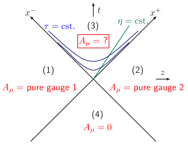
Figure 1: Color fields in spacetime. In regions (1) and (2), where only one of the nuclei has passed by, the field is the pure gauge field of this one nucleus. In region (3) the field is known numerically.

The sheet of color charge is approximated as infinitesimal, but its physical size can be estimated by renormalization group arguments. Let us concentrate on the nucleus moving along the $x^{-}=0$-lightcone. There is a cutoff $\Lambda^{+}$ separating the hard and soft degrees of freedom. The degrees of freedom with $p^{+}\gtrsim\Lambda^{+}$ are described as classical color charges and the ones with $k^{+}\lesssim\Lambda^{+}$ as classical fields, characterized by the saturation scale $Q_{\mathrm{s}}$. The renormalization group equation for this system describes how the distribution of color charges evolves when the cutoff is changed. When $\Lambda^{+}$ changes by a factor $e^{\Delta y}$, the correction to the saturation scale is of order $\alpha_{\mathrm{s}}\Delta y$ and becomes of order one only when $\Delta y\sim 1/\alpha_{\mathrm{s}}$. When studying the soft degrees of freedom around midrapidity $y\sim\eta\sim 0$ we can therefore assume that they are separated from the sources with $p^{+}\gtrsim\Lambda^{+}$ by a rapidity difference $\Delta y\sim 1/\alpha_{\mathrm{s}}$. The characteristic momentum and time scales for these soft modes at $y\sim 0$ are $k^{+}\sim Q_{\mathrm{s}}$ and $\Delta\tau\sim 1/Q_{\mathrm{s}}$. These soft classical fields see hard sources as localized in an interval $\Delta z\sim\Delta x^{-}\sim 1/p^{+}\lesssim e^{-1/\alpha_{\mathrm{s}}}/Q_{\mathrm{s}}$ which, being close to the $x^{-}=0$-lightcone (see Fig. 1), corresponds to a time interval $\Delta\tau\sim e^{-1/\alpha_{\mathrm{s}}}/Q_{\mathrm{s}}$. The smallness, in the weak coupling limit, of this scale $e^{-1/\alpha_{\mathrm{s}}}/Q_{\mathrm{s}}$ compared to the scale $1/Q_{\mathrm{s}}$ of the soft fields is the physical picture approximated by the infinitesimally thin sheet.

For the collision of two nuclei, we imagine working in the center of mass frame. Here the two nuclei can be thought of as sheets of colored glass. The fields associated with the collision are illustrated in Fig.1. We choose the fields to vanish in the backward light cone. On the side light cones, we choose the fields to be two dimensional pure gauge transforms of vacuum,

$$A^{i}_{(1,2)}=\frac{1}{ig}U_{(1,2)}\nabla^{i}U^{\dagger}_{(1,2)}\vspace{-.5cm}$$ (2.1)

The derivatives are two dimensional and transverse in the sheets. The discontinuity of the field at $x^{\pm}=0$ in the backward light cone is determined by the source density on the two sheets,

$$J^{\mu}=\delta^{\mu+}\delta(x^{-})\rho_{1}(\mathbf{x}_{T})+\delta^{\mu-}\delta(x^{+})\rho_{2}(\mathbf{x}_{T})\vspace{-.5cm}$$ (2.2)

In practice, to relate the vector potential to the charge density, one has to spread the charge density out in the longitudinal space, but this does not affect the determination of the solution of the classical field in terms of the vector potentials $A^{i}_{(1,2)}$.

In Fig. 2, the classical color and magnetic fields are shown on the two nuclei before the collision. They are frozen in time and the color electric and color magnetic fields are orthogonal to the beam direction and to one another.

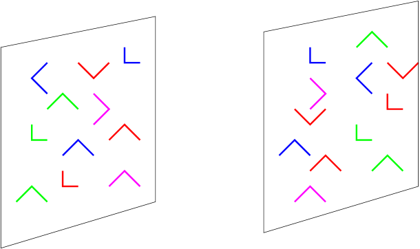
Figure 2: The fields on the two nuclei prior to the collision.

In the forward light cone, there is no solution which is pure gauge. There is therefore particle production and evolution in the forward lightcone. This matter is the Glasma, until it eventually evolves into a thermalized Quark Gluon Plasma. Because the sources, Eq. 2.2, are restricted to the light cone there is a boost invariant solution of the field equations in the forward light cone. It is convenient to work in the $\tau,\eta$ coordinate system and in radial gauge,

$$A_{\tau}=\frac{1}{\tau}\left(x^{+}A^{-}+x^{-}A^{+}\right)=0.\vspace{-.5cm}$$ (2.3)

The field can then be written in terms of $\alpha\equiv A^{\eta}$ and the transverse components as

$$A^{\pm} = \pm x^{\pm}\alpha(\tau,x_{T})$$

$$A^{i} = \alpha_{3}^{i}(\tau,x_{T}).\vspace{-.5cm}$$ (2.4)

The equations of motion for these fields were written explicitly in [1, 2]. As second order partial differential equations they require initial conditions for the fields and the first time derivatives. These boundary conditions at $\tau=0$ are determined by requiring that the Yang Mills equations be solved across the forward lightcone, and are

$$\alpha_{3}^{i}\mid_{\tau=0} = \alpha^{i}_{1}+\alpha^{i}_{2}$$

$$\alpha\mid_{\tau=0} = \frac{ig}{2}\left[\alpha^{i}_{1},\alpha^{i}_{2}\right]$$

$${\partial_{\tau}}\alpha\mid_{\tau=0} = {\partial_{\tau}}\alpha_{3}^{i}\mid_{\tau=0}=0.\vspace{-.5cm}$$ (2.5)

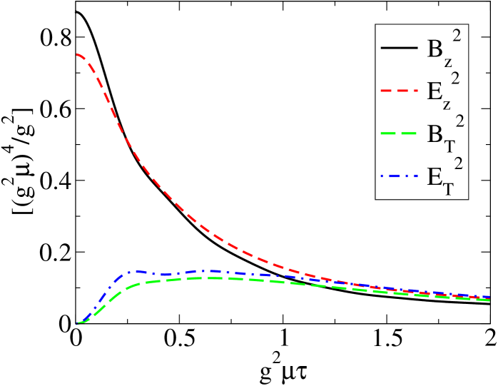
Figure 3: Components of the gauge field, computed numerically on a $512^{2}$-lattice with $g^{2}\mu R_{A}=67.7$.

If one then solves the Yang-Mills equation near the light cone, one finds that the transverse color electric and color magnetic fields vanish as $\tau\rightarrow 0$, but that the longitudinal electric and magnetic fields are non-vanishing [39, 40],

$$E^{z} = ig[\alpha^{i}_{1},\alpha^{i}_{2}]$$

$$B^{z} = ig\epsilon^{ij}[\alpha^{i}_{1},\alpha^{j}_{2}].$$ (2.6)

A plot of the transverse and longitudinal color fields is shown in Fig.3, based on a numerical solution of these equations.

A picture of the fields after the collision is shown in Fig. 4, at a time infinitesimal after the collision. In addition to the fields in the sheet, there are longitudinal electric and magnetic fields, which are random in color with a correlation length scale in the transverse plane of order $\mathcal{O}(1/Q_{\mathrm{s}})$. There are new sources of color electric and magnetic charge on the sheets on which the original fields resided.

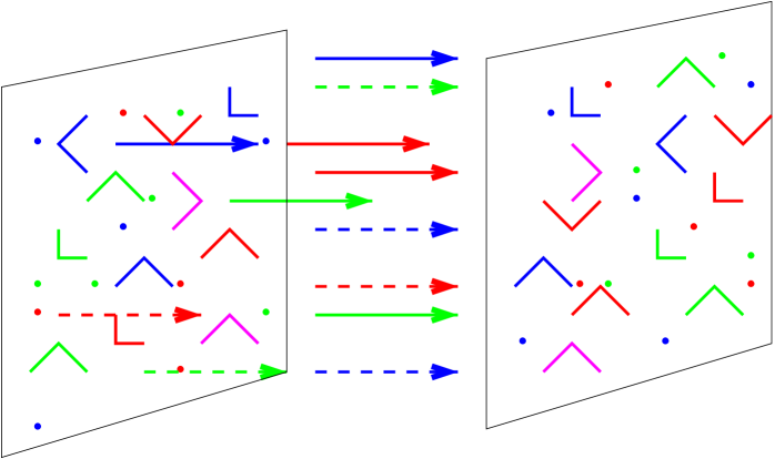
Figure 4: The color electric and magnetic fields after the collision. In addition to the transverse fields on the sheets there is a longitudinal field between them, originating from electric and magnetic charges on the sheets.

The presence of the longitudinal fields is at first sight surprising. How did the longitudinal electric and magnetic field arise? Let us define the chromoelectric and chromomagnetic charge densities by

$$\nabla\cdot\vec{E} = \rho_{\mathrm{electric}}$$

$$\nabla\cdot\vec{B} = \rho_{\mathrm{magnetic}}.\vspace{-.5cm}$$ (2.8)

Because the fields satisfy the nonabelian Gauss law and the Bianchi identity these charge densities have a contribution from the gauge field itself:

$$\rho_{\mathrm{electric}} = ig[A^{i},E^{i}]$$

$$\rho_{\mathrm{magnetic}} = ig[A^{i},B^{i}].\vspace{-.5cm}$$ (2.9)

The source terms turn on instantaneously in the forward light cone. This arises because there are transverse electric and magnetic fields in the sheets, which in the forward light cone are multiplied by a non-vanishing vector potential from the opposing sheet. The induced charge density on one sheet is the negative of that on the other, as it must be to generate the longitudinal magnetic and electric fields and be consistent with Gauss’s law. To be explicit, the nucleus on the $x^{-}=0$ light cone has a gauge potential $A^{i}=\theta(x^{-})\alpha^{i}_{1}(\mathbf{x}_{T})$ and the other nucleus $A^{i}=\theta(x^{+})\alpha^{i}_{2}(\mathbf{x}_{T})$. The cross terms of these two give rise to the opposite charges on the light cones, electric

$$\rho_{\mathrm{electric}}=\frac{ig}{\sqrt{2}}\theta(x^{-})\delta(x^{+})[\alpha^{i}_{1},\alpha^{i}_{2}]+\frac{ig}{\sqrt{2}}\theta(x^{+})\delta(x^{-})[\alpha^{i}_{2},\alpha^{i}_{1}]\vspace{-.5cm}$$ (2.10)

and magnetic

$$\rho_{\mathrm{magnetic}}=\frac{ig}{\sqrt{2}}\theta(x^{-})\delta(x^{+})\epsilon^{ij}[\alpha^{i}_{1},\alpha^{j}_{2}]+\frac{ig}{\sqrt{2}}\theta(x^{+})\delta(x^{-})\epsilon^{ij}[\alpha^{j}_{1},\alpha^{i}_{2}],\vspace{-.5cm}$$ (2.11)

which exactly correspond to the initial longitudinal fields, Eq. (2).

After the collisions, sources of magnetic and electric charge have appeared on the sheets. The valence structure of the nuclei have changed, and there are new sources for the fields. This description is very similar in spirit to the original suggestions for a string based description of heavy ion collisions. These old pictures had only sources of electric charge [41, 42, 43, 44]. The appearance of a longitudinal magnetic field is an entirely new aspect.

In the Lund Monte Carlo model [41], there are longitudinal electric fields induced by a collision, which subsequently decay by quantum pair production. The situation here is similar except for the longitudinal magnetic field and the different length scale in the transverse direction, $1/Q_{\mathrm{s}}$ in stead of $1/\Lambda_{\mathrm{QCD}}$. The other essential difference is that the fields can decay away by classical evolution of the charged Yang-Mills field. There is not a necessity for pair production from quantum effects to quench the fields. We will expand on this later, since, the quantum and classical quenching processes are related in a non-trivial way.

It is interesting to note the structure of the energy momentum tensor $T_{\mu\nu}=\frac{1}{4}g_{\mu\nu}F^{\alpha\beta}F_{\alpha\beta}-F_{\mu}{}^{\alpha}F_{\nu\alpha}$ for this initial condition. It is diagonal and, as always in gauge theory, traceless: $T_{\mu\nu}={\textstyle\frac{1}{2}}(E_{z}^{2}+B_{z}^{2})\times\mathrm{diag}(1,-1,-1,1)$. This can be compared to the standard form for a system with an anisotropy in the $z$-direction: $T_{\mu\nu}=\mathrm{diag}(\epsilon,-p_{\perp},-p_{\perp},-p_{L}),$ where $\epsilon$ is the energy density and $p_{\perp}$ and $p_{L}$ are the transverse and longitudinal pressures. We see that the initial field configuration has negative “longitudinal pressure”. The configuration that is the starting point for studies of isotropization by plasma instabilities, where the diagonal elements of $T_{\mu\nu}$ at $\eta=0$ are $(\epsilon,-\epsilon/2,-\epsilon/2,0)$, is only reached at times $\tau\gtrsim 1/Q_{\mathrm{s}}$ when the classical fields start to behave linearly due to the expansion of the system.

Finally, the non-zero longitudinal electric and magnetic fields implies that the initial conditions have a large density of topological charge $F^{\mu\nu}\widetilde{F}_{\mu\nu}$. Since

$$\partial^{\mu}K_{\mu}=F^{\mu\nu}\widetilde{F}_{\mu\nu}\vspace{-.5cm}$$ (2.12)

there is also a nonzero Chern-Simons current. We will investigate the topology of these configurations in the next section. The physical picture we have of the initial conditions looks quite similar to that proposed by Kharzeev, Kovchegov and Levin [30] and by Janik, Shuryak and Zahed [47, 48], who claimed that high energy collisions might be described by the decay of instanton like configurations, the sphalerons. The decay of these longitudinal electric and magnetic fields is in fact the decay of topological charge.

To thermalize the system, one must first produce quanta associated with the gluon field. In order to be described as quanta, the classical field associated with these quanta must be weak, $A\ll 1/g$. For a mode with momentum $p_{T}$, this occurs in a time of order $\tau\sim 1/p_{T}$. For a time $1/p_{T}\ll\tau\ll 1/(\alpha_{S}p_{T})$, the field has strength $1\ll A\ll 1/g$, and can be treated either classically, or as an ensemble of particles. This follows because, up to oscillations, the field behaves as $1/\sqrt{\tau}$ at late times. For $p_{T}\gg 1/(\alpha_{S}\tau)$, the field is essentially quantum, as the classical field is small compared to the field induced by quantum fluctuations (see [52] for an argument approaching this same limit from the opposite direction, i.e. kinetic theory, and [53, 54] for a more formal argument).

Roughly speaking, the emission of particles occurs during the time interval $1/Q_{\mathrm{s}}\ll\tau\ll 1/(\alpha_{\mathrm{s}}Q_{\mathrm{s}})$. Since $\alpha_{\mathrm{s}}$ varies logarithmically with $Q_{\mathrm{s}}$, the time scale is crudely $1/Q_{\mathrm{s}}$. Nevertheless, this treatment suggests there is an intermediate time scale where either the classical and transport solutions to the evolution of a coupled system of fields and particles may be a good approximation. Above the high momentum end of this matching interval, one should use a hard particle treatment. Below the lower scale of the overlap region, one should use a classical field treatment. For a complete treatment, one should have a floating scale which depends upon time. Modes above this floating scale are hard particles, and those below are soft.

The picture is therefore of classical fields evaporating into gluons, and a system where the hard gluons are interacting with a classical field. The interaction of the hard gluons among themselves is probably not so important during the time interval $1/Q_{\mathrm{s}}\ll\tau\ll 1/(\alpha_{\mathrm{s}}Q_{\mathrm{s}})$ since the characteristic time scale for hard particles to thermalize by interactions among themselves is of order $\tau\sim 1/(\alpha_{\mathrm{s}}^{2}Q_{\mathrm{s}})$, since these interactions involve scattering cross sections. The interaction of the classical field with itself is important, and the characteristic time scale for interaction of the hard fields with the classical fields is also important, since the effects of coupling constant cancel out in the interactions of the hard field with the coherent fields strength $A\sim 1/g$.

It is this system which we refer to as the Glasma.

An issue of current interest is whether or not the boost invariant solution described in the previous section is stable with respect to space-time rapidity dependent fluctuations. There is reasonably strong evidence that the coupled particle–field Glasma system has such instabilities. The issue of the purely classical evolution also has claims that this may be the case [37], but they happen over extremely long time scale, and one may be worried about whether such instabilities reflect the continuum limit.

As we will discuss in Sec. 3, the topological properties of the gauge fields depend crucially on the dimensionality of the system. One would therefore expect that relaxing the strict boost invariance of the field configurations will significantly change the dynamics of the Chern-Simons charge. Perhaps the instability of the boost invariant Glasma and the production of net topological charge might be related.

If the purely classical system is unstable, then one may legitimately worry about the validity of the entire Glasma description. The problem is that if the instability is like that of classical turbulence, then different initial conditions which are separated from one another infinitesimally, will at late times evolve to solutions far apart with $\Delta S\sim S$ . Such a difference in initial conditions might be generated by quantum noise. Their contribution to the path integral will differ by a factor of

$$e^{i\Delta S}\vspace{-.5cm}$$ (2.13)

which is oscillatory. Therefore one would not expect convergence of the glassy sum over initial conditions.

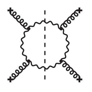
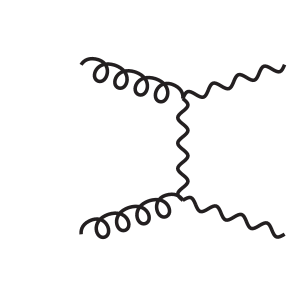
Figure 5: Left: A lowest order (both in the classical field and in the quantum corrections) diagram that contributes to the imaginary part of the effective action. The winding lines represent the classical field, $\mathcal{O}(1/g)$ and the wavy lines the quantum fluctuation, $\mathcal{O}(1)$. Right: The corresponding pair production diagram.

There can also be instabilities with $\Delta S\sim\alpha_{\mathrm{s}}S\ll S$. In addition to the interpretation of the momentum modes of the classical field as gluonic quanta there is quantum radiation. This may be generated by considering the small fluctuations in the classical time dependent background field. The effective action is then obtained by integrating over these fluctuations. At fourth order in the expansion of the effective action in powers of the external field, there is an imaginary part generated, coming from diagrams such as the one in Fig. 5. This imaginary part is precisely pair production. Pair production does not correspond to an instability of the purely classical equations, but to an instability of the classical background field in a quantum mechanical treatment. It remains an effect suppressed by $\alpha_{\mathrm{s}}$ with respect to the classical background and is therefore not a problem for the validity of the glassy description. A consistent computation of this pair production must also include the renormalization group evolution of the classical fields, which contributes at the same order in $\alpha_{\mathrm{s}}$ [55]. Kharzeev, Levin and Tuchin [45, 46] have argued that for fields of the type we have shown exist in the collision of two sheets of colored glass, specifically a pulsed longitudinal electric field, the distribution of produced particles is an exponential in transverse mass, contributing to the early thermalization of the system.

The contribution to the gluon multiplicity from pair production is related to the diagram shown in Fig. 5, where one integrates over one of the legs of the quantum fluctuation field. In this integration the integral over $\Delta y$, the rapidity gap between the produced gluons, diverges (see e.g. Appendix B of [56]). The region $\Delta y\gtrsim 1/\alpha_{\mathrm{s}}$ corresponds to renormalization group evolution of the sources and the genuine quantum correction to gluon production only comes from the region $\Delta y\ll 1/\alpha_{\mathrm{s}}$. To compute the first quantum correction to gluon production one must introduce a cutoff $Y\sim 1/\alpha_{\mathrm{s}}$ in the integration over $\Delta y$. One then integrates over one of the legs in Fig. 5 up to this cutoff. The physical result is independent of $Y$, because the dependence of the gluon multiplicity on $Y$ must be cancelled by the renormalization group evolution of the sources as a function of $Y$. Thus pair production remains suppressed by a power of $\alpha_{\mathrm{s}}$ compared to the background field. This can be contrasted with the calculation of quark pair production [57, 58, 59, 60], where the integral over $\Delta y$ is convergent and the quark multiplicity is directly suppressed by $\alpha_{\mathrm{s}}$ compared to the classical field. Quark pairs, unlike gluons, do not contribute to the renormalization group evolution of the source to this order.

3 Topological Charge

The topological charge density of a gauge field configuration is defined as

$$\frac{\mathrm{d}^{4}\nu}{\mathrm{d}x^{4}}=\frac{g^{2}}{32\pi^{2}}{\rm Tr}\widetilde{F}^{\mu\nu}F_{\mu\nu}=\frac{g^{2}}{8\pi^{2}}{\rm Tr}\vec{E}\cdot\vec{B},\vspace{-.5cm}$$ (3.14)

where $\widetilde{F}^{\mu\nu}={\textstyle\frac{1}{2}}\epsilon^{\mu\nu\rho\sigma}F_{\rho\sigma}$. The charge density is the four-divergence of the topological current, $\widetilde{F}_{a}^{\mu\nu}F^{a}_{\mu\nu}=\partial_{\mu}K^{\mu}$, where

$$K^{\mu}=\epsilon^{\mu\nu\rho\sigma}A^{a}_{\nu}\left(F^{a}_{\rho\sigma}+\frac{g}{3}f^{abc}A^{b}_{\rho}A^{c}_{\sigma}\right).\vspace{-.5cm}$$ (3.15)

Integrating the 0-component of the current over space one can define a topological charge $\nu=\frac{g^{2}}{64\pi^{2}}\int\mathrm{d}^{3}\mathbf{x}K^{0}$. The change in the topological charge between times,

$$\nu(t\to\infty)-\nu(t\to-\infty)=\int\mathrm{d}t\partial_{t}\nu=\frac{g^{2}}{32\pi^{2}}\int\mathrm{d}^{4}x{\rm Tr}\widetilde{F}^{\mu\nu}F_{\mu\nu},\vspace{-.5cm}$$ (3.16)

is a gauge invariant quantity, but the topological current and charge themselves are gauge dependent. It is therefore essential in our case that one cannot transform away the pure gauge contribution at large $\tau$, because such a gauge transformation would introduce in the backward lightcone a nonzero gauge potential $A_{i}$.

Working in the boost invariant case it is more natural to look at the Chern-Simons charge per unit rapidity on a constant proper time surface

$$\frac{\mathrm{d}\nu}{\mathrm{d}\eta}=\frac{g^{2}}{64\pi^{2}}\int\mathrm{d}^{2}\mathbf{x}_{T}\tau K_{\tau}=\frac{g^{2}}{64\pi^{2}}\int\mathrm{d}^{2}\mathbf{x}_{T}\epsilon^{ij}\left[A^{a}_{\eta}\left(F^{a}_{ij}+gf^{abc}A^{b}_{i}A^{c}_{j}\right)+2A^{a}_{i}F^{a}_{j\eta}\right]\vspace{-.5cm}$$ (3.17)

As was pointed out in [31] this expression can be written in a much simpler form when the field configurations are boost invariant. Performing a partial integration one can rearrance Eq. (3.17) as

$$\frac{\mathrm{d}\nu}{\mathrm{d}\eta}=\frac{g^{2}}{32\pi^{2}}\int\mathrm{d}^{2}\mathbf{x}_{T}\epsilon^{ij}A^{a}_{\eta}F^{a}_{ij}=\frac{g^{2}}{16\pi^{2}}\int\mathrm{d}^{2}\mathbf{x}_{T}A^{a}_{\eta}B^{az}.\vspace{-.5cm}$$ (3.18)

The surface term from the partial integration is

$$\frac{g^{2}}{32\pi^{2}}\int\mathrm{d}^{2}\mathbf{x}_{T}\epsilon^{ij}\partial_{j}\left(A^{a}_{i}A^{a}_{\eta}\right)=\frac{g^{2}}{32\pi^{2}}\oint\mathrm{d}x^{i}A^{a}_{i}A^{a}_{\eta}.\vspace{-.5cm}$$ (3.19)

There should be a large topological charge density associated with the Glasma. This is because the Glasma fields at $\tau\to 0^{+}$ have longitudinal $\vec{E}$ and $\vec{B}$ and give nonvanishing $\vec{E}\cdot\vec{B}$. Of course, the typical correlation length in these fields in transverse size is the saturation momentum, and for reasons described below, we expect zero total Chern-Simons charge from these fields. It is interesting that this resembles the situation envisioned by Kharzeev, Kovchegov and Levin [30] and Janik, Shuryak and Zahed [47, 48] in that the production of particles can be thought of as due to the decay of Chern-Simons charge. Presumably, this is somewhat like the situation at finite temperature where one has a density of sphalerons associated with the decay of topological charge. It is amusing here that the topological charge density arises already at the classical level and is $\mathcal{O}(1)$, not $\mathcal{O}(\alpha_{\mathrm{s}})$ as it would be from quantum fluctuations.

For early times the electric and magnetic fields are both longitudinal, and there is a nonzero topological charge density. Note that because $\mathrm{d}/\mathrm{d}\eta=\tau\mathrm{d}/\mathrm{d}z$ the charge density per unit rapidity is zero, but the density per unit $z$ nonzero. The expectation value of the Chern-Simons charge density when averaged over the source color charge densities is zero, but the magnitude of the fluctuations, $\sqrt{\left\langle\left(\mathrm{d}\nu/\mathrm{d}\eta\right)^{2}\right\rangle}$, can be estimated as follows. The system consists of approximately $N=\pi R_{A}^{2}Q_{\mathrm{s}}^{2}$ uncorrelated domains, each having charge $\sim 1$. The sum of these independent charges will fluctuate around zero with magnitude $\sqrt{\left\langle\left(\mathrm{d}\nu/\mathrm{d}\eta\right)^{2}\right\rangle}\sim\sqrt{N}\sim Q_{\mathrm{s}}R_{A}$. This estimate is confirmed by the numerical calculation [31].

For late times $\tau\to\infty$ the field gets weak due to the expansion of the system and the gauge field can be written as a gauge transformation of a solution to the linearized equations of motion [2]. The general such asymptotic form of the solution is:

$$A_{i} = V(\mathbf{x}_{T})\left(\epsilon_{i}(\mathbf{x}_{T},\tau)-\frac{i}{g}\partial_{i}\right)V^{\dagger}(\mathbf{x}_{T})$$

$$A_{\eta} = V(\mathbf{x}_{T})\epsilon(\mathbf{x}_{T},\tau)V^{\dagger}(\mathbf{x}_{T})\vspace{-.5cm}$$ (3.20)

with

$$\epsilon_{i}(\mathbf{x}_{T},\tau) = \int\frac{\mathrm{d}^{2}{\mathbf{k}_{T}}}{(2\pi)^{2}}e^{i{\mathbf{k}_{T}}\cdot\mathbf{x}_{T}}\left[J_{0}(|{\mathbf{k}_{T}}|\tau)h^{J}_{i}({\mathbf{k}_{T}})+N_{0}({\mathbf{k}_{T}}\tau)h^{N}_{i}({\mathbf{k}_{T}})\right]$$

$$\epsilon(\mathbf{x}_{T},\tau) = \int\frac{\mathrm{d}^{2}{\mathbf{k}_{T}}}{(2\pi)^{2}}e^{i{\mathbf{k}_{T}}\cdot\mathbf{x}_{T}}\tau\left[J_{1}(|{\mathbf{k}_{T}}|\tau)h^{J}({\mathbf{k}_{T}})+N_{1}({\mathbf{k}_{T}}\tau)h^{N}({\mathbf{k}_{T}})\right].\vspace{-.5cm}$$ (3.21)

This decomposition between the field and the pure gauge contribution is not unique, but this ambiguity can be removed by requiring that $\epsilon_{i}$ satisfies the transversal Coulomb gauge condition $\partial_{i}\epsilon_{i}=0$. The mode functions $h^{J}_{i}({\mathbf{k}_{T}}),h^{N}_{i}({\mathbf{k}_{T}}),h^{J}({\mathbf{k}_{T}}),h^{N}({\mathbf{k}_{T}})$ are determined by the nonlinear dynamics of the system at early times.

In the lowest order perturbative solution [2] the mode functions are determined only by the initial conditions. Because the Neumann functions $N_{n}$ diverge at the origin, $h^{N}_{i}({\mathbf{k}_{T}})$ and $h^{N}({\mathbf{k}_{T}})$ vanish at in the lowest order. Thus the Chern-Simons charge, Eq. 3.18, for each transverse momentum mode behaves as $J_{0}(|{\mathbf{k}_{T}}|\tau)J_{1}(|{\mathbf{k}_{T}}|\tau)$, giving a zero contribution when averaging over a time period $\tau\gg 1/|{\mathbf{k}_{T}}|$. At higher orders in the source also the Neumann function solutions can be present and $h^{N}_{i}({\mathbf{k}_{T}})$ and $h^{N}({\mathbf{k}_{T}})$ can be finite. Because $J_{0}(|{\mathbf{k}_{T}}|\tau)N_{1}(|{\mathbf{k}_{T}}|\tau)$ and $N_{0}(|{\mathbf{k}_{T}}|\tau)J_{1}(|{\mathbf{k}_{T}}|\tau)$ oscillate around finite values, these terms can give a finite radiative contribution to the topological charge. This higher order radiative contribution is the most likely interpretation for the finite topological charge seen in the numerical calculation [31].

When, as in Ref. [31], the topological charge is computed on a finite lattice with periodic boundary conditions and thus the surface term Eq. (3.19) vanishes exactly. In general it is possible to have a solution where the combination of a covariantly constant longitudinal field $A_{\eta}=V(\mathbf{x}_{T})\epsilon V^{\dagger}(\mathbf{x}_{T})$ with ${\partial_{\tau}}\epsilon=\partial_{i}\epsilon=0$ and the pure gauge component $V(\mathbf{x}_{T})$ give a nonvanishing topological charge. This contribution is not present in the perturbative solution of Ref. [2], because a constant $A_{\eta}$ corresponds to $A^{\eta}$ that diverges at $\tau=0$ and is not allowed by the initial condition. For an arbitrary color charge distribution in the transverse plane the pure gauge fields of the individual nuclei, and thus also the pure gauge fields in the asymptotical solution Eq. (3), vanish only logarithmically for large $\mathbf{x}_{T}$. However the overall color charge of the nucleus must be zero, and thus for distances larger than $1/\Lambda_{\mathrm{QCD}}$ outside the nucleus the color field must die off faster, meaning that the boundary term will vanish.

3.1 Homotopy Groups

The $n$th homotopy group $\pi_{n}(G)$ of a topological space $G$, in our case the gauge or symmetry group, is the group of mappings from the $n$-sphere $S^{n}$ to $G$. The usefulness of homotopy groups in field theory often arises in the following way. Let us presume were are interested in a field theory with symmetry group $G$. When one requires that field configurations in $R^{n}$ approach a constant at large distances, one can view space as the compact group $S^{n}$. The homotopy group $\pi_{n}(G)$ then tells us whether topologically inequivalent field configurations exist. One example is the group $\pi_{2}(\textrm{O(3)})=\mathbb{Z}$, which tells us that in an O(3)-symmetric nonlinear sigma model in 2 dimensions one can construct a topological charge that takes integer values [61]. Another example is the Skyrme model [62, 63], where the solitons of an SU(2) symmetric “pion” field in three dimensions can be interpreted as having integer baryon number, because $\pi_{3}(\textrm{SU(2)})=\mathbb{Z}$. For this same reason the Chern-Simons number of SU(3) in a gauge theory changes by an integer in a nonperturbatively large gauge transformation. The second homotopy group of SU(3), however, is trivial: $\pi_{2}(\textrm{SU(3)})=0$, meaning that for boost invariant two dimensional field configurations one can not construct a topological charge taking integer values.

4 Conclusions

We have in this paper tried to elucidate some known but little appreciated aspects of Glasma, the highly coherent matter making in transition from Color Glass Condensate to Quark Gluon Plasma. It is characterized, in a manner reminiscent of the Lund model, by the decay of a longitudinal electric and magnetic field into particles. This decay can happen both as classical radiation of the field and, quantum pair production from the classical background. We have discussed the relation of these two processes and pointed out that a full computation of the pair production must be done consistently with the renormalization group evolution of the sources.

As the magnetic and electric fields are initially parallel, they correspond to a nonzero Chern-Simons charge density. The evolution of the Glasma can thus be described also as the decay of this Chern-Simons charge.

References

- [1] A. Kovner, L.D. McLerran and H. Weigert, Phys. Rev. D52 (1995) 6231, hep-ph/9502289.
- [2] A. Kovner, L.D. McLerran and H. Weigert, Phys. Rev. D52 (1995) 3809, hep-ph/9505320.
- [3] M. Gyulassy and L.D. McLerran, Phys. Rev. C56 (1997) 2219, nucl-th/9704034.
- [4] Y.V. Kovchegov and D.H. Rischke, Phys. Rev. C56 (1997) 1084, hep-ph/9704201.
- [5] A. Krasnitz and R. Venugopalan, Nucl. Phys. B557 (1999) 237, hep-ph/9809433.
- [6] A. Krasnitz and R. Venugopalan, Phys. Rev. Lett. 84 (2000) 4309, hep-ph/9909203.
- [7] A. Krasnitz and R. Venugopalan, Phys. Rev. Lett. 86 (2001) 1717, hep-ph/0007108.
- [8] A. Krasnitz, Y. Nara and R. Venugopalan, Phys. Rev. Lett. 87 (2001) 192302, hep-ph/0108092.
- [9] T. Lappi, Phys. Rev. C67 (2003) 054903, hep-ph/0303076.
- [10] L.V. Gribov, E.M. Levin and M.G. Ryskin, Phys. Rept. 100 (1983) 1.
- [11] A.H. Mueller and J.W. Qiu, Nucl. Phys. B268 (1986) 427.
- [12] L.D. McLerran and R. Venugopalan, Phys. Rev. D49 (1994) 2233, hep-ph/9309289.
- [13] L.D. McLerran and R. Venugopalan, Phys. Rev. D49 (1994) 3352, hep-ph/9311205.
- [14] L.D. McLerran and R. Venugopalan, Phys. Rev. D50 (1994) 2225, hep-ph/9402335.
- [15] E. Iancu, A. Leonidov and L.D. McLerran, Nucl. Phys. A692 (2001) 583, hep-ph/0011241.
- [16] E. Ferreiro et al., Nucl. Phys. A703 (2002) 489, hep-ph/0109115.
- [17] A. Dumitru and L.D. McLerran, Nucl. Phys. A700 (2002) 492, hep-ph/0105268.
- [18] J.P. Blaizot, F. Gelis and R. Venugopalan, Nucl. Phys. A743 (2004) 13, hep-ph/0402256.
- [19] J.P. Blaizot, F. Gelis and R. Venugopalan, Nucl. Phys. A743 (2004) 57, hep-ph/0402257.
- [20] D. Kharzeev, E. Levin and L. McLerran, Phys. Lett. B561 (2003) 93, hep-ph/0210332.
- [21] J. Jalilian-Marian, Y. Nara and R. Venugopalan, Phys. Lett. B577 (2003) 54, nucl-th/0307022.
- [22] D. Kharzeev, Y.V. Kovchegov and K. Tuchin, Phys. Rev. D68 (2003) 094013, hep-ph/0307037.
- [23] D. Kharzeev, Y.V. Kovchegov and K. Tuchin, Phys. Lett. B599 (2004) 23, hep-ph/0405045.
- [24] R. Baier, A. Kovner and U.A. Wiedemann, Phys. Rev. D68 (2003) 054009, hep-ph/0305265.
- [25] J.L. Albacete et al., Phys. Rev. Lett. 92 (2004) 082001, hep-ph/0307179.
- [26] E. Iancu, K. Itakura and D.N. Triantafyllopoulos, Nucl. Phys. A742 (2004) 182, hep-ph/0403103.
- [27] A. Dumitru, A. Hayashigaki and J. Jalilian-Marian, Nucl. Phys. A765 (2006) 464, hep-ph/0506308.
- [28] D. Kharzeev, R.D. Pisarski and M.H.G. Tytgat, Phys. Rev. Lett. 81 (1998) 512, hep-ph/9804221.
- [29] D. Kharzeev and R.D. Pisarski, Phys. Rev. D61 (2000) 111901, hep-ph/9906401.
- [30] D.E. Kharzeev, Y.V. Kovchegov and E. Levin, Nucl. Phys. A699 (2002) 745, hep-ph/0106248.
- [31] D. Kharzeev, A. Krasnitz and R. Venugopalan, Phys. Lett. B545 (2002) 298, hep-ph/0109253.
- [32] S. Mrowczynski, Phys. Rev. C49 (1994) 2191.
- [33] S. Mrowczynski, Phys. Lett. B393 (1997) 26, hep-ph/9606442.
- [34] P. Arnold, J. Lenaghan and G.D. Moore, JHEP 08 (2003) 002, hep-ph/0307325.
- [35] P. Romatschke and M. Strickland, Phys. Rev. D68 (2003) 036004, hep-ph/0304092.
- [36] P. Romatschke and M. Strickland, Phys. Rev. D70 (2004) 116006, hep-ph/0406188.
- [37] P. Romatschke and R. Venugopalan, Phys. Rev. Lett. 92 (2006) 062302, hep-ph/0510121.
- [38] STAR, I.V. Selyuzhenkov, (2005), nucl-ex/0510069.
- [39] R.J. Fries, J.I. Kapusta and Y. Li, (2005), hep-ph/0511101.
- [40] R.J. Fries, J.I. Kapusta and Y. Li, “Near Field Expansion of the Color Glass Condensate in High Energy Nuclear Collisions,” NUC-MINN-06/2-T, in preparation.
- [41] B. Andersson et al., Phys. Rept. 97 (1983) 31.
- [42] H. Ehtamo, J. Lindfors and L.D. McLerran, Z. Phys. C18 (1983) 341.
- [43] T.S. Biro, H.B. Nielsen and J. Knoll, Nucl. Phys. B245 (1984) 449.
- [44] G. Gatoff, A.K. Kerman and T. Matsui, Phys. Rev. D36 (1987) 114.
- [45] D. Kharzeev and K. Tuchin, Nucl. Phys. A753 (2005) 316, hep-ph/0501234.
- [46] D. Kharzeev, E. Levin and K. Tuchin, (2006), hep-ph/0602063.
- [47] R.A. Janik, E. Shuryak and I. Zahed, Phys. Rev. D67 (2003) 014005, hep-ph/0206005.
- [48] E. Shuryak and I. Zahed, Phys. Rev. D67 (2003) 014006, hep-ph/0206022.
- [49] F. Schrempp, (2005), hep-ph/0507160.
- [50] F. Schrempp and A. Utermann, (2004), hep-ph/0401137.
- [51] F. Schrempp and A. Utermann, Phys. Lett. B543 (2002) 197, hep-ph/0207300.
- [52] R. Baier et al., Phys. Lett. B502 (2001) 51, hep-ph/0009237.
- [53] A.H. Mueller and D.T. Son, Phys. Lett. B582 (2004) 279, hep-ph/0212198.
- [54] S. Jeon, Phys. Rev. C72 (2005) 014907, hep-ph/0412121.
- [55] F. Gelis and R. Venugopalan, (2006), hep-ph/0601209.
- [56] A. Leonidov and D. Ostrovsky, Phys. Rev. D62 (2000) 094009, hep-ph/9905496.
- [57] F. Gelis and R. Venugopalan, Phys. Rev. D69 (2004) 014019, hep-ph/0310090.
- [58] H. Fujii, F. Gelis and R. Venugopalan, Phys. Rev. Lett. 95 (2005) 162002, hep-ph/0504047.
- [59] F. Gelis, K. Kajantie and T. Lappi, Phys. Rev. C71 (2005) 024904, hep-ph/0409058.
- [60] F. Gelis, K. Kajantie and T. Lappi, Phys. Rev. Lett. 96 (2006) 032304, hep-ph/0508229.
- [61] E. Mottola and A. Wipf, Phys. Rev. D39 (1989) 588.
- [62] T.H.R. Skyrme, Proc. Roy. Soc. Lond. A260 (1961) 127.
- [63] G.S. Adkins, C.R. Nappi and E. Witten, Nucl. Phys. B228 (1983) 552.