We study the transverse-momentum distribution of hadrons produced in semi-inclusive deep-inelastic scattering (SIDIS). We consider cross sections for various combinations of polarizations of the initial lepton and nucleon or the produced hadron, for which we perform the resummation of large double-logarithmic perturbative corrections arising at small transverse momentum. We present phenomenological results for the processes $lp\to l\pi X$ with longitudinally polarized leptons and protons. We discuss the impact of the perturbative resummation and of estimated non-perturbative contributions on the corresponding cross sections and their spin asymmetry. Our results should be relevant for ongoing studies in the COMPASS experiment at CERN, and for future experiments at the proposed eRHIC collider at BNL.

1 Introduction

Our knowledge about the structure of hadrons has been vastly improved by experiments with polarized high-energy lepton beams scattering off polarized nucleon targets. Spin observables in deeply-inelastic lepton-nucleon collisions allow us to extract the spin-dependent parton distributions of the nucleon. At the same time, they challenge our understanding of the reaction mechanism within QCD, and our ability to perform reliable theoretical calculations of the relevant cross sections for each process and kinematic region of interest.

Of particular interest in this respect are observables in semi-inclusive deeply-inelastic scattering (SIDIS), $lp\to lhX$, for which a hadron $h$ is detected in the final state. Depending on the type of hadron considered, various different aspects of nucleon structure may be probed. Two current lepton scattering experiments, HERMES at DESY and COMPASS at CERN, employ this method extensively. Measurements of spin asymmetries for longitudinally polarized beam and target, integrated over all transverse momenta of the produced hadron, have served to allow conclusions about the helicity-dependent up, down, and strange quark and anti-quark distributions in the nucleon [1]. It has also been recognized that distributions in the hadron’s transverse momentum can be of great interest, in particular when the nucleon target is transversely polarized [2]. The associated experimental investigations by HERMES [3], COMPASS [4], the SMC [5], and CLAS [6] have been remarkably productive and have opened windows on novel QCD phenomena such as the Sivers [7] and Collins [8] effects. It is hoped that experiments at a possibly forthcoming polarized electron-proton collider, eRHIC, would carry on and extend these studies [9].

Theoretically, the most interesting kinematic regime is characterized by large virtuality $Q^{2}$ of the photon exchanged in the DIS process, and relatively small transverse momentum, $q_{T}\ll Q$. This regime also provides for the bulk of the events in experiment. It is precisely here, for example, that effects related to intrinsic transverse momenta of partons in the nucleon may become visible, potentially offering new insights into nucleon structure. At the same time, the theoretical analysis of hard-scattering in this regime is fairly involved, but well-understood. In particular, the emission of gluons from the DIS Born process $\gamma^{\ast}q\to q$ also leads to non-vanishing transverse-momentum of the final-state hadron and needs to be taken into account appropriately. It is the goal of this paper to present state-of-the-art calculations for the transverse-momentum dependence of some SIDIS observables. For this study, we will focus entirely on the set of leading-twist double-spin reactions,

$${\rm(i)} \quad e+p\rightarrow e+\pi+X\;,$$ (1)

$${\rm(ii)} \quad e+\vec{p}\rightarrow e+\vec{\Lambda}+X\;,$$

$${\rm(iii)} \quad e+{p}^{\uparrow}\rightarrow e+{\Lambda}^{\uparrow}+X\;,$$

$${\rm(iv)} \quad\vec{e}+\vec{p}\rightarrow e+\pi+X\;,$$

$${\rm(v)} \quad\vec{e}+p\rightarrow e+\vec{\Lambda}+X\;.$$

Here arrows to the right (upward arrows) denote longitudinal (transverse) polarization. Needless to say that the final-state pion could be replaced by any hadron. The same is true for the $\Lambda$, as long as the observed hadron is spin-1/2 and its polarization can be detected experimentally. In our study, we will make use of several ingredients available in the literature. In an earlier publication [10], two of us presented results for the $2\to 3$ partonic reactions $lq\to lqg$ and $lg\to lq\bar{q}$, for all polarizations of interest. In the perturbative expansion and using collinear factorization, these processes are the first to yield a non-vanishing transverse momentum of the produced hadron. In terms of the strong coupling $\alpha_{s}$ they are of order ${\cal O}(\alpha_{s})$. We therefore refer to them as “leading order (LO)” processes for the hadron transverse-momentum distribution. They are expected to be adequate (at least qualitatively) for achieving a good theoretical description at large transverse momentum, $q_{T}\sim Q$. In the unpolarized case, the complete next-to-leading (NLO) (${\cal O}(\alpha_{s}^{2})$) corrections to the $q_{T}$-distribution have been calculated [11, 12, 13] which will lead to an improvement of the theoretical calculation at large $q_{T}$. 

At low transverse momentum, $q_{T}\ll Q$, fixed-order calculations are bound to fail. The reason for this is well understood: when $q_{T}\to 0$, gluon emission is inhibited, and the cancellation of infra-red singularities between real and virtual diagrams in the perturbative series leaves behind logarithmic remainders of the form

$$\alpha_{S}^{k}\,\frac{\ln^{m}\left(Q^{2}/q_{T}^{2}\right)}{q_{T}^{2}}$$ (2)

in the cross section $d\sigma/dq_{T}^{2}$ at the $k$th order of perturbation theory, where $m=1,\ldots,2k-1$. Ultimately, when $q_{T}\ll Q$, $\alpha_{s}$ will not be useful anymore as the expansion parameter in the perturbative series since the logarithms will compensate for the smallness of $\alpha_{s}$. Accordingly, in order to obtain a reliable estimate for the cross section, one has to sum up (“resum”) the large logarithmic contributions to all orders in $\alpha_{s}$. Techniques for this resummation are well established, starting with pioneering work mostly on the Drell-Yan process in the late 1970’s to mid 1980’s [18, 19, 20, 21, 22]. The “Collins-Soper-Sterman” (CSS) formalism [22] has become the standard method for $q_{T}$ resummation. It is formulated in impact-parameter ($b$) space, which guarantees conservation of the soft-gluon transverse momenta. The formalism has also been applied to the unpolarized SIDIS cross section [23, 24], and it was found [24] that data for $q_{T}$ distributions from the HERA $ep$ collider [25, 26] are satisfactorily described.

Resummations at small transverse momentum $q_{T}$ have also been developed for spin observables. In Refs. [27, 28] the CSS formalism was applied to longitudinal and transverse double-spin asymmetries in the Drell-Yan process. Early resummation studies on $q_{T}$-distributions in jet production in polarized DIS were performed in [29]. In Ref. [30, 31] leading-logarithmic (LL) resummation effects were investigated for spin asymmetries that involve transverse-momentum dependent distributions, in particular the Collins functions mentioned above. In Ref. [32], resummation formulas for polarized SIDIS were derived, based on a factorization theorem at low transverse momentum [33]. A main result of [32] is that the CSS evolution equation is the same for the spin-dependent cases as in the unpolarized one. Knowing the expression for the unpolarized resummed cross section, and the complete polarized LO cross sections [10], it is then relatively straightforward to determine the resummed expressions for the polarized case. These will be provided in explicit form in this paper, for the cases listed in (1). We shall present results corresponding to resummation to next-to-leading logarithmic (NLL) accuracy, which corresponds to resummation of the towers with $2k-1,2k-2,2k-3$ in (2). We shall also present numerical estimates for the reaction $\vec{e}\vec{p}\to e\pi X$ at COMPASS and eRHIC, in order to study the general features of the resummation and its impact on the cross sections and the spin asymmetry. We note that in the numerical evaluation one needs to specify a recipe for treating the integration over the impact parameter at very large $b\sim 1/\Lambda_{\rm QCD}$, in order to avoid the Landau pole present in the resummed expression. This is closely related to non-perturbative effects generated by resummation [22, 34, 35, 36, 37, 38, 39]. We will use two different methods for treating the large $b$-region.

We stress that we will not address single-transverse spin phenomena in this paper like those related to the Sivers and Collins effects mentioned above. For these, the analysis of QCD radiative effects is rather more involved [31] than for the double-spin case we consider, in particular regarding the connection of the behavior at small and large transverse momentum $q_{T}$ [40]. Also, as we shall see below, the $q_{T}$-differential cross section in general contains terms depending on the angle $\phi$ between the hadron and lepton planes. We shall only consider the resummation of the $\phi$-independent pieces in the cross section, which dominate at small $q_{T}$. It is an interesting topic by itself to study the resummation of the terms that depend on $\phi$ [41].

The remainder of this paper is organized as follows: Section 2 provides all formulas needed for the $q_{T}$-differential SIDIS cross section, at LO and for the NLL resummed case. In section 3, we present numerical estimates for $\vec{e}\vec{p}\to e\pi X$ at COMPASS and eRHIC, based on the resummation formulas. We discuss in particular the effect of the resummation on the spin asymmetry. We also study the impact of the treatment of the large-$b$ region and of non-perturbative corrections on the resummed cross sections and the spin asymmetry. We conclude in Sec. 4. In the Appendix, we list the complete $O(\alpha_{s})$ cross sections for the processes in (1), correcting some typos in [10].

2 The $q_{T}$-differential SIDIS cross section

2.1 Kinematics

We are interested in the cross section for the process

$$\vec{l}(k)+A(p_{A},S_{A})\rightarrow l(k^{\prime})+B(p_{B},S_{B})+X\;,$$ (3)

where $S_{A},S_{B}$ are the spin vectors for the initial nucleon and the produced final-state hadron, which can be longitudinal or transverse, as indicated in (1). The lepton can be unpolarized or longitudinally polarized; transverse-spin effects for the lepton are suppressed by $m_{l}/Q$ because of chirality conservation at the lepton-photon vertex and hence are negligible. From now on, we will for definiteness take hadron $A$ to be a proton and the lepton $l$ to be an electron. We define five Lorentz invariants, denoted $S_{ep},x_{bj},Q^{2},z_{f}$, and $q_{T}^{2}$, to describe the process. The center of mass energy squared, $S_{ep}$, for the initial electron and the proton is

$$S_{ep}=(p_{A}+k)^{2}\simeq 2p_{A}\cdot k\;,$$ (4)

ignoring masses. The conventional DIS variables are defined in terms of the virtual photon momentum $q=k-k^{\prime}$ as

$$x_{bj}={Q^{2}\over 2p_{A}\cdot q}\;,\qquad Q^{2}=-q^{2}=-(k-k^{\prime})^{2}\;,$$ (5)

and they may be determined experimentally by observing the scattered electron. For the final-state hadron $B$, we introduce the scaling variable

$$z_{f}={p_{A}\cdot p_{B}\over p_{A}\cdot q}\;.$$ (6)

Finally, we define the “transverse” component of $q$, which is orthogonal to both $p_{A}$ and $p_{B}$:

$$q_{t}^{\mu}=q^{\mu}-{p_{B}\cdot q\over p_{A}\cdot p_{B}}p_{A}^{\mu}-{p_{A}\cdot q\over p_{A}\cdot p_{B}}p_{B}^{\mu}\;.$$ (7)

$q_{t}$ is a space-like vector, and we denote its magnitude by

$$q_{T}=\sqrt{-q_{t}^{2}}\;.$$ (8)

To completely specify the kinematics, we need to choose a reference frame. We shall work in the so-called hadron frame [42, 43], which is the Breit frame of the virtual photon and the initial proton:

$$q^{\mu} = (0,0,0,-Q)\;,$$ (9)

$$p_{A}^{\mu} = \left({Q\over 2x_{bj}},0,0,{Q\over 2x_{bj}}\right)\;.$$ (10)

Further, in this frame the outgoing hadron $B$ is taken to be in the $xz$ plane:

$$p_{B}^{\mu}={z_{f}Q\over 2}\left(1+{q_{T}^{2}\over Q^{2}},{2q_{T}\over Q},0,{q_{T}^{2}\over Q^{2}}-1\right)\;.$$ (11)

As one can see, the transverse momentum of hadron $B$ is in this frame given by $z_{f}q_{T}$. This is true for any frame in which the 3-momenta of the virtual photon and the initial proton are collinear. By introducing the angle $\phi$ between the hadron plane and the lepton plane, the lepton momentum can be parameterized as

$$k^{\mu}={Q\over 2}\left(\cosh\psi,\sinh\psi\cos\phi,\sinh\psi\sin\phi,-1\right)\;,$$ (12)

and one finds

$$\cosh\psi={2x_{bj}S_{eA}\over Q^{2}}-1\;.$$ (13)

For the case (iii) in (1) [$ep^{\uparrow}\to e\Lambda^{\uparrow}X$] when the initial proton is transversely polarized and the transverse polarization of an outgoing spin-1/2 hadron is observed, we need to parameterize the spin vectors $S_{A\perp}$ and $S_{B\perp}$ to lie in the planes orthogonal to $\vec{p}_{A}$ and $\vec{p}_{B}$, respectively. In the hadron frame, they can be written as

$$S_{A\perp}^{\mu} = (0,\cos\Phi_{A},\sin\Phi_{A},0)\;,$$

$$S_{B\perp}^{\mu} = (0,\cos\Theta_{B}\cos\Phi_{B},\sin\Phi_{B},-\sin\Theta_{B}\cos\Phi_{B})\;,$$ (14)

so that $\Phi_{A,B}$ are the azimuthal angles of $S_{A,B\perp}$ around $\vec{p}_{A,B}$ as measured from the hadron plane and $\Theta_{B}$ is the polar angle of $\vec{p}_{B}$ measured with respect to $\vec{p}_{A}$. One finds:

$$\cos\Theta_{B}={q_{T}^{2}-Q^{2}\over q_{T}^{2}+Q^{2}},\qquad\sin\Theta_{B}={2q_{T}Q\over q_{T}^{2}+Q^{2}}\;.$$ (15)

We note that the polarization state depends on the frame we choose. For example, a state that is transversely polarized in the hadron frame becomes a mixture of longitudinally polarized and transversely polarized states in the laboratory frame where the initial electron and proton are collinear. With the above definitions, the cross section for (3) can be expressed in terms of $S_{ep}$, $x_{bj}$, $Q^{2}$, $z_{f}$, $q_{T}^{2}$ and $\phi$ in the hadron frame. Note that $\phi$ is invariant under boosts in the $\vec{q}$-direction, so that is the same in the hadron frame and, for example, in the photon-proton center-of-mass frame.

2.2 Structure of the lowest-order cross section

The complete set of the $O(\alpha_{s})$ spin-dependent partonic cross sections for large-$q_{T}$ hadron production in SIDIS have been derived in Ref. [10]. They are obtained from the Feynman diagrams for the reactions $lq\to lqg$ and $lg\to lq\bar{q}$. For completeness, and for the reader’s convenience, we list them in the Appendix. Here we summarize the main characteristics of the hadronic cross section.

The cross section can be decomposed into several pieces with different $\phi$-dependences:

$${d^{5}\sigma\over dQ^{2}dx_{bj}dz_{f}dq_{T}^{2}d\phi}=\sigma_{0}+{\rm cos}(\phi)\sigma_{1}+{\rm cos}(2\phi)\sigma_{2}\;,$$ (16)

for processes (i) and (ii) in (1),

$${d^{5}\sigma\over dQ^{2}dx_{bj}dz_{f}dq_{T}^{2}d\phi}=\sigma_{0}+{\rm cos}(\phi)\sigma_{1}\;,$$ (17)

for (iv) and (v), and

$${d^{5}\sigma_{T}\over dQ^{2}dx_{bj}dz_{f}dq_{T}^{2}d\phi}=\cos(\Phi_{A}-\Phi_{B}-2\phi)\sigma_{0}^{T}+\cos(\Phi_{A}-\Phi_{B}-\phi)\sigma_{1}^{T}+\cos(\Phi_{A}-\Phi_{B})\sigma_{2}^{T}\;,$$ (18)

for (iii). In the hadron frame, $\sigma_{0}$ and $\sigma_{0}^{T}$ in these decompositions behave as $\alpha_{s}\ln\left(Q^{2}/q_{T}^{2}\right)/q_{T}^{2}$ at small $q_{T}$. This is the manifestation of the large logarithmic corrections described in the Introduction at this order. At yet higher orders, corrections as large as $\alpha_{S}^{k}\,\ln^{2k}\left(Q^{2}/q_{T}^{2}\right)/q_{T}^{2}$ in the cross section arise. In the following, we will study the NLL resummation of these large logarithmic corrections within the CSS formalism. We note that the other components of the cross sections in Eqs. (16)-(18) are less singular as $q_{T}\to 0$: $\sigma_{1}$ and $\sigma_{1}^{T}$ behave as $\alpha_{s}\ln\left(Q^{2}/q_{T}^{2}\right)/q_{T}$, and $\sigma_{2}$ and $\sigma_{2}^{T}$ as $\alpha_{s}\ln\left(Q^{2}/q_{T}^{2}\right)$. These pieces too, however, receive large higher-order corrections at small $q_{T}$ [23] and would need to be resummed [41]. In this paper we will only focus on the resummation for $\sigma_{0}$ and $\sigma_{0}^{T}$.

2.3 Asymptotic part of the lowest-order cross section

We will now discuss the behavior of the cross sections at small $q_{T}$ in more detail. This is a first step in arriving at the resummed cross section. Following [23, 24], we write the cross section at $O(\alpha_{s})$ as

$${d^{5}\sigma^{\rm LO}\over dQ^{2}dx_{bj}dz_{f}dq_{T}^{2}d\phi}={d^{5}\sigma^{\rm asymp}\over dQ^{2}dx_{bj}dz_{f}dq_{T}^{2}d\phi}+Y(S_{ep},Q,q_{T},x_{bj},z_{f})\;,$$ (19)

where the first term on the right-hand-side is the “asymptotic” part in $\sigma_{0}$ and $\sigma_{0}^{T}$ containing the pieces that are singular as $\ln\left(Q^{2}/q_{T}^{2}\right)/q_{T}^{2}$ or $1/q_{T}^{2}$ at small $q_{T}$, while $Y$ collects the remainder which is at most logarithmic as $q_{T}\to 0$. It is straightforward to derive the asymptotic part of the LO unpolarized SIDIS cross section from the expressions in the Appendix. One finds:

$${d^{5}\sigma^{\rm asymp}\over dQ^{2}dx_{bj}dz_{f}dq_{T}^{2}d\phi} = {\alpha_{em}^{2}\alpha_{s}\over 8\pi x_{bj}^{2}S_{ep}^{2}Q^{2}}\,{\cal A}_{1}\,\frac{2Q^{2}}{q_{T}^{2}}\,\sum_{q,\bar{q}}\,e_{q}^{2}\left[2f_{q}(x_{bj},\mu)D_{q}(z_{f},\mu)\left(C_{F}\ln\left({Q^{2}\over q_{T}^{2}}\right)-{3\over 2}C_{F}\right)\right.$$

$$+\,\left\{f_{q}(x_{bj},\mu)\otimes P^{\,in,(0)}_{qq}+f_{g}(x_{bj},\mu)\otimes P_{qg}^{\,in,(0)})\right\}D_{q}(z_{f},\mu)\,$$

$$+\;f_{q}(x_{bj},\mu)\left\{P_{qq}^{\,out,(0)}\otimes D_{q}(z_{f},\mu)+P_{gq}^{\,out,(0)}\otimes D_{g}(z_{f},\mu)\right\}\Bigg{]}\;,$$ (20)

where $\alpha_{em}$ is the electromagnetic coupling constant, $e_{q}$ the fractional quark charge, and $C_{F}=4/3$. ${\cal A}_{1}$ is defined in (A.2). In Eq. (20), $f_{q}(x,\mu)$ and $f_{g}(x,\mu)$ denote, respectively, the unpolarized quark and gluon distribution functions for the proton at scale $\mu$, and $D_{q}(z,\mu)$ and $D_{g}(z,\mu)$ are quark and gluon fragmentation functions for the produced hadron. Furthermore, for the unpolarized cross section, the $P_{ij}^{\,in,(0)}$ and $P_{ij}^{\,out,(0)}$ are identical, and they are equal to the customary LO unpolarized splitting functions: $P_{ij}^{\,in,(0)}=P_{ij}^{\,out,(0)}\equiv P_{ij}^{(0)}$, where

$$P_{qq}^{(0)}(x) = C_{F}\left[{1+x^{2}\over(1-x)_{+}}+{3\over 2}\delta(1-x)\right]\;,$$

$$P_{gq}^{(0)}(x) = C_{F}{1+(1-x)^{2}\over x}\;,$$

$$P_{qg}^{(0)}(x) = T_{R}\,\left[x^{2}+(1-x)^{2}\right]\;.$$ (21)

Here, $T_{R}=1/2$, and the “+”-prescription in the first line acts in an integral from $x$ to 1 as

$$\int_{x}^{1}dy\frac{f(y)}{(1-y)_{+}}=\int_{x}^{1}dy\frac{f(y)-f(1)}{1-y}+f(1)\ln(1-x)\;,$$ (22)

for any suitably regular function $f$. Finally, the symbol $\otimes$ denotes convolutions of the forms

$$f_{q}(x_{bj},\mu)\otimes P_{qq}^{\,in(0)}\equiv\int_{x_{bj}}^{1}{dx\over x}f_{q}(x,\mu)P_{qq}^{\,in,(0)}\left(\frac{x_{bj}}{x}\right)\;,$$

$$P_{qq}^{\,out,(0)}\otimes D_{q}(z_{f},\mu)\equiv\int_{z_{f}}^{1}{dz\over z}P_{qq}^{\,out,(0)}(z)D_{q}\left(\frac{z_{f}}{z},\mu\right)\;.$$ (23)

For the other processes listed in (1), the asymptotic parts are obtained in the same manner from the cross sections given in Appendix A. They can be cast in the form (20) with the following replacements:

(ii) $e\vec{p}\to e\vec{\Lambda}X$:

$$f_{q}\to\Delta f_{q},\qquad f_{g}\to\Delta f_{g},\qquad D_{q}\to\Delta D_{q},\qquad D_{g}\to\Delta D_{g}\;,$$ (24)

where the $\Delta f_{q}$, $\Delta f_{g}$ and $\Delta D_{q}$, $\Delta D_{g}$ denote the helicity-dependent quark and gluon parton densities and fragmentation functions, respectively (for definitions, see [2]). Furthermore,

$$P_{ij}^{\,in,(0)}\to\Delta P_{ij}^{(0)}\;,\quad P_{ij}^{\,out,(0)}\to\Delta P_{ij}^{(0)}\;,$$ (25)

with

$$\Delta P_{qq}^{(0)}(x)=P_{qq}^{(0)}(x)\;,\quad\Delta P_{gq}^{(0)}(x)=C_{F}\left[2-x\right]\;,\quad\Delta P_{qg}^{(0)}(x)=T_{R}\left[2x-1\right]\;.$$ (26)

(iii) $e{p}^{\uparrow}\to e{\Lambda}^{\uparrow}X$:

$${\cal A}_{1}\to\sinh^{2}\psi\cos(\Phi_{A}-\Phi_{B}-2\phi)\;,$$

$$f_{q}\to\delta f_{q}\;,\qquad f_{g}\to 0\;,\qquad D_{q}\to\delta D_{q}\;,\qquad D_{g}\to 0\;,$$

$$P_{qq}^{\,in,(0)}\to\delta P_{qq}^{(0)}\;,\qquad P_{qq}^{\,out,(0)}\to\delta P_{qq}^{(0)}\;.$$ (27)

Here, the $\delta f_{q}$ and $\delta D_{q}$ denote the transversity distribution and fragmentation functions, respectively. As is well-known, gluons do not contribute to transversity at leading twist [2]. The LO transversity splitting function is given by

$$\delta P_{qq}^{(0)}(x)=C_{F}\left[{2x\over(1-x)_{+}}+{3\over 2}\delta(1-x)\right].$$ (28)

(iv) $\vec{e}\vec{p}\to e{\Lambda}X$:

$${\cal A}_{1}\to{\cal-A}_{6}\;,\qquad f_{q}\to\Delta f_{q}\;,\qquad f_{g}\to\Delta f_{g}\;,$$

$$P_{ij}^{\,in,(0)}\to\Delta P_{ij}^{(0)}\;,\qquad P_{ij}^{\,out,(0)}\to P_{ij}^{(0)}\;.$$ (29)

(v) $\vec{e}{p}\to e\vec{\Lambda}X$:

$${\cal A}_{1}\to{\cal-A}_{6}\;,\qquad D_{q}\to\Delta D_{q}\;,\qquad D_{g}\to\Delta D_{g}\;,$$

$$P_{ij}^{\,in,(0)}\to P_{ij}^{(0)}\;,\qquad P_{ij}^{\,out,(0)}\to\Delta P_{ij}^{(0)}\;.$$ (30)

2.4 NLL resummed cross section

Resummation of the small-$q_{T}$ logarithms is achieved in impact-parameter ($b$) space, where the large corrections exponentiate. In $b$-space, the leading logarithms $\alpha_{S}^{k}\,\ln^{2k-1}\left(Q^{2}/q_{T}^{2}\right)/q_{T}^{2}$ turn into $\alpha_{s}^{k}\ln^{2k}(bQ/b_{0})$, where $b_{0}=2{\mathrm{e}}^{-\gamma_{E}}$ with $\gamma_{E}$ being the Euler constant. Subleading logarithms are down by one or more powers of $\ln(bQ/b_{0})$. In the following, we will present the resummation formulas for the processes (i)-(v) in (1) we are interested in, based on the CSS formalism [22] (see also [23, 24, 32]). We will make some standard choices [22] for the parameters and scales in that formalism, which render the resulting expressions as simple and transparent as possible.

For the unpolarized resummed cross one has

$${d\sigma^{res}\over dx_{bj}dz_{f}dQ^{2}dq_{T}^{2}d\phi}={\pi\alpha_{em}^{2}\over 2x_{bj}^{2}S_{ep}^{2}}\,{\cal A}_{1}\int{d^{2}\vec{b}\over(2\pi)^{2}}\,{\mathrm{e}}^{i\vec{b}\cdot\vec{q}_{T}}\,W(b,Q,x_{bj},z_{f})\;,$$ (31)

where the $b$-space expression for the resummed cross section $W$ is given by

$$W(b,Q,x_{bj},z_{f})=\!\!\!\!\!\!\sum_{\begin{array}[]{c}j=q,\bar{q}\\ i,k=q,\bar{q},g\end{array}}\!\!\!\!\!\!\!\!\!e_{j}^{2}\,\left[f_{i}(x_{bj},b_{0}/b)\otimes C_{ji}^{\,in}\right]\,\times\,{\mathrm{e}}^{S(b,Q)}\times\left[C_{kj}^{\,out}\otimes D_{k}(z_{f},b_{0}/b)\right]\;,$$ (34)

the convolutions being defined as in Eqs. (23). As indicated, the scale in the parton distributions is given by $\mu=b_{0}/b$. We will return to this in the next subsection.

The Sudakov form factor $S(b,Q)$ in Eq. (34) reads

$$S(b,Q)=-\int_{b_{0}^{2}/b^{2}}^{Q^{2}}{dk_{T}^{2}\over k_{T}^{2}}\left[A\left(\alpha_{s}(k_{T})\right)\ln\left({Q^{2}\over k_{T}^{2}}\right)+B\left(\alpha_{s}(k_{T})\right)\right]\;,$$ (35)

where the functions $A$ and $B$ have perturbative expansions of the form

$$A\left(\alpha_{s}\right)=\sum_{k=1}^{\infty}A_{k}\left({\alpha_{s}\over\pi}\right)^{k}\;,\quad B\left(\alpha_{s}\right)=\sum_{k=1}^{\infty}B_{k}\left({\alpha_{s}\over\pi}\right)^{k}.$$ (36)

For the resummation at NLL, one needs the coefficients $A_{1,2}$ and $B_{1}$, which read [34, 44]:

$$A_{1}=C_{F}\;,\quad A_{2}=\frac{1}{2}\;C_{F}\left[C_{A}\left(\frac{67}{18}-\frac{\pi^{2}}{6}\right)-\frac{5}{9}N_{f}\right]\;,\quad B_{1}=-\frac{3}{2}C_{F}\;,$$ (37)

The functions $C_{ij}^{\,in}$ and $C_{ij}^{\,out}$ in Eq. (34) are also perturbative. Their expansions read

$$C^{\,in/out}_{ij}(x,\alpha_{s}(\mu)) = \sum_{k=0}^{\infty}C^{\,in/out,(k)}_{ij}(x)\left({\alpha_{s}(\mu)\over\pi}\right)^{k}\;.$$ (38)

Here $\mu$ is a renormalization scale of order $Q$. The LO coefficients are given by

$$C^{\,in,(0)}_{qq^{\prime}}(x) = \delta_{qq^{\prime}}\delta(1-x)\;,\qquad C^{\,out,(0)}_{qq^{\prime}}(z)=\delta_{qq^{\prime}}\delta(1-z)\;,$$

$$C^{\,in,(0)}_{qg} = C^{\,out,(0)}_{gq}=0\;.$$ (39)

The first-order coefficients $C^{\,in/out,(1)}_{ij}$ could be obtained by expanding Eq. (34) to $O(\alpha_{s})$, performing an inverse Fourier transform, and comparing to the fixed-order (${\cal O}(\alpha_{s})$) $q_{T}$ distribution. The asymptotic part we have given in Eq. (20) alone is not sufficient for this because it does not contain the contributions $\propto\delta^{2}(\vec{q}_{T})$ at ${\cal O}(\alpha_{s})$. Fortunately, the coefficients are known in the literature, and have a very transparent structure in the $\overline{\mathrm{MS}}$ scheme [24, 43] (see also work on the coefficients in the related Drell-Yan case in [21, 34, 45]). One has:

$$C^{\,in,(1)}_{ij}(x)=-{1\over 2}P^{\,in,\epsilon}_{ij}(x)+\delta_{ij}{\cal C}_{\delta}\delta(1-x)\;,$$ (40)

$$C^{\,out,(1)}_{ij}(z)=-{1\over 2}P^{\,out,\epsilon}_{ij}(z)+\ln(z)P_{ij}^{out,(0)}(z)+\delta_{ij}{\cal C}_{\delta}\delta(1-z)\;.$$ (41)

Here the $P^{\,in,\epsilon}_{ij}(x)$, $P^{\,out,\epsilon}_{ij}(x)$ are the terms $\propto\epsilon$ in the LO splitting functions in $d=4-2\epsilon$ dimensions, $P_{ij}^{\,in/out,(0)}(x,\epsilon)$, and are defined through

$$P_{ij}^{\,in/out,(0)}(x,\epsilon)=P_{ij}^{in/out,(0)}(x)+\epsilon P_{ij}^{\,in/out,\epsilon}(x)\;.$$ (42)

The usual splitting functions in $d=4$ dimensions have been given above in Eqs. (21). One has [46]

$$P_{qq}^{\,\epsilon}(x)=-C_{F}\left[1-x-\frac{1}{2}\delta(1-x)\right]\;,\;\;\;P_{qg}^{\,\epsilon}(x)=-2T_{R}x(1-x)\;,\;\;\;P_{gq}^{\,\epsilon}(x)=-C_{F}x\;.$$ (43)

Furthermore, the coefficient ${\cal C}_{\delta}$ in Eqs. (40),(41) arises from hard virtual corrections. It is therefore only present for the case $ij=qq$, where ${\cal C}_{\delta}=-7C_{F}/4$. Finally, for the “final-state” coefficient $C^{\,out,(1)}_{ij}$ there is an extra contribution $\propto\ln z$ [24, 43] times the LO splitting function. It is of kinematic origin and contributed by the phase space for collinear gluon radiation off the quark leg in the final state [49].

With this, the formulas for the resummation of the unpolarized SIDIS cross section in $b$-space are complete. It is now straightforward to extend them to the various spin-dependent cross sections in (1). The Sudakov form factors are entirely related to soft-gluon emission and hence are spin-independent and the same in each case [32]. For each process, we first need to make the appropriate replacements as described above in Eqs. (24)-(30). In addition, we obtain the respective coefficients $C_{ij}^{\,in/out,(1)}$ from Eqs. (40),(41), substituting appropriately all splitting functions, and also the $P_{ij}^{\,in/out,\epsilon}$ by the $\propto\epsilon$ terms in the $d=4-2\epsilon$-dimensional versions of the LO splitting functions that (24)-(30) direct us to use. For this we need the $\propto\epsilon$ terms in the spin-dependent splitting functions. For longitudinal polarization we have [47]

$$\Delta P_{qq}^{\,\epsilon}(x)=-C_{F}\left[1-x-\frac{1}{2}\delta(1-x)\right]\;,$$

$$\Delta P_{qg}^{\,\epsilon}(x)=-2T_{R}(1-x)\;,\;\;\Delta P_{gq}^{\,\epsilon}(x)=2C_{F}(1-x)\;.$$ (44)

In case of transversity, the splitting function in $4-2\epsilon$ dimensions is for $x<1$ identical to that in four dimensions [48], so that

$$\delta P_{qq}^{\,\epsilon}(x)=\frac{C_{F}}{2}\delta(1-x)\;.$$ (45)

The coefficient ${\cal C}_{\delta}$ for the case $ij=qq$ in Eqs. (40),(41) is the same for all polarized cases, since it comes from virtual diagrams.

Knowledge of the coefficients $A_{1,2}$, $B_{1}$ and $C_{ij}^{(0),(1)}$ in Eqs. (31),(34) is sufficient for the resummation to NLL accuracy. For consistency, we also need to use the two-loop expression for the strong running coupling, and the NLO evolution for the parton densities and fragmentation functions. Let us finally give an explicit formula for the NLL expansion of the Sudakov form factor. Defining

$$L=\ln\left(1+Q^{2}b^{2}/b_{0}^{2}\right)\;,$$ (46)

and choosing the renormalization scale $\mu$, we have [50]:

$$S(Q,b)={1\over\alpha_{s}(\mu)}f_{0}(\alpha_{s}(\mu)L)+f_{1}(\alpha_{s}(\mu)L)\;,$$ (47)

where

$$f_{0}(y) = {A_{1}\over\pi\beta_{0}^{2}}\left[\beta_{0}y+\ln(1-\beta_{0}y)\right],$$ (48)

$$f_{1}(y) = {A_{1}\beta_{1}\over\pi\beta_{0}^{3}}\left[{1\over 2}\ln^{2}(1-\beta_{0}y)+{\beta_{0}y\over 1-\beta_{0}y}+{\ln(1-\beta_{0}y)\over 1-\beta_{0}y}\right]+{B_{1}\over\pi\beta_{0}}\ln(1-\beta_{0}y)$$ (49)

$$+\frac{1}{\pi\beta_{0}}\left[A_{1}\ln\left(\frac{Q^{2}}{\mu^{2}}\right)-{A_{2}\over\pi\beta_{0}}\right]\left[\ln(1-\beta_{0}y)+{\beta_{0}y\over 1-\beta_{0}y}\right]\;,$$

with the coefficients of the QCD $\beta$-function $\beta_{0}=(33-2N_{f})/(12\pi)$ and $\beta_{1}=(153-19N_{F})/(24\pi^{2})$. We observe that as $y\to 0$, $f_{0}(y)={\cal O}(y^{2})$ and $f_{1}(y)={\cal O}(y)$. Note that in Eq. (46) we have followed Ref. [51] to choose $\ln\left(1+Q^{2}b^{2}/b_{0}^{2}\right)$ rather than $\ln\left(Q^{2}b^{2}/b_{0}^{2}\right)$ as the large logarithm in $b$-space. As far as the large-$b$ behavior and NLL resummation are concerned, the two are equivalent, of course. With the choice in (46), however, the Sudakov exponent vanishes at $b=0$, as it should [19, 21, 22], whereas for the other choice it gives large logarithms not only at large $b$ (small $q_{T}$) but also artificially at small $b$ (large $q_{T}$). For further discussion, see [51].

2.5 Evolution of parton distributions and fragmentation
functions

As we have seen in Eq. (34), in the CSS formalism the parton distributions and fragmentation functions are evaluated at the factorization scale $\mu=b_{0}/b$. As discussed in [37], it then becomes a great convenience to treat them in Mellin-moment space, because this enables one to explicitly express their evolution between a large scale $\sim Q$ and $b_{0}/b$. In this way, one avoids the problem normally faced in $q_{T}$ resummation that one needs to call the parton densities or fragmentation functions at scales far below their range of validity (see below), so that some sort of “freezing” (or related prescription) for handling them is required. We also anticipate that below we will choose the impact parameter $b$ to be complex-valued, so that it becomes desirable to separate the complex scale $b_{0}/b$ from the scale at which the parton densities are explicitly evaluated.

To be more specific, we write the resummed cross section as $W(b,Q,x_{bj},z_{f})$ in Eq. (34) as an inverse Mellin transform of moments in $x_{bj}$ and $z_{f}$:

$$W(b,Q,x_{bj},z_{f}) = \!\!\!\!\!\!\sum_{\begin{array}[]{c}j=q,\bar{q}\\ i,k=q,\bar{q},g\end{array}}\!\!\!\!\!\!\!\!\!e_{j}^{2}\,\left({1\over 2\pi i}\right)^{2}\int_{{{\cal C}}_{N}}\,dN\,\int_{{{\cal C}}_{M}}\,dM\,z_{f}^{-M}x_{bj}^{-N}$$ (53)

$$\hskip 42.67912pt\times\,f_{i}^{N}(b_{0}/b)C_{ji}^{\,in,N}{\mathrm{e}}^{S(b,Q)}C_{kj}^{\,out,M}D_{k}^{M}(b_{0}/b)\;,$$

where the moment of each function is defined as

$$f^{N}_{i}(\mu)\equiv\int_{0}^{1}\,x^{N-1}f_{i}(x,\mu)\;,\qquad C^{\,in,N}_{ji}(\alpha_{s}(\mu))\equiv\int_{0}^{1}\,x^{N-1}C^{\,in}_{ji}(x,\alpha_{s}(\mu))\;,$$ (54)

and so forth. The integrations over $N$ and $M$ in Eq. (53) are over contours in the complex plane, to be chosen in such a way that they lie to the right of the rightmost singularities of the parton distributions and the fragmentation functions. In moment space, it is possible to express the moments $f_{i}^{N}(b_{0}/b)$ and $D_{k}^{M}(b_{0}/b)$ by the corresponding moments at scale $\sim Q$. The evolution “factor” between the scales $b_{0}/b$ and $Q$ (which in general is a matrix because of singlet mixing) can be written in closed analytical form and can be expanded to NLL accuracy in $L$. One then only needs the parton densities and fragmentation functions at scale $Q$. For further details, see [37].

2.6 Inverse Fourier transform and non-perturbative corrections

As shown in Eq. (31), the resummed cross section in $q_{T}$-space is obtained by an inverse Fourier transform of $W(b,Q,x_{bj},z_{f})$. This involves an integration over $b=|\vec{b}|$ from 0 to $\infty$. Because of the Landau pole of the perturbative strong coupling in the Sudakov exponent (35) at $k_{T}=\Lambda_{\mathrm{QCD}}$, this integration is ill-defined. In the expansion (47) for the Sudakov form factor, the singularity occurs at $\beta_{0}\alpha_{s}(\mu)L=1$. In other words, the $b$-integration extends over both perturbative ($b\ll 1/\Lambda_{QCD}$) and non-perturbative ($b\leq 1/\Lambda_{QCD}$ or even larger) regions. In order to define a perturbative resummed cross section, a prescription for the $b$ integration is required that avoids the Landau pole. The ambiguity in the perturbative series implied by the presence of the Landau pole corresponds to a non-perturbative correction. One may therefore use resummation to examine the structure of non-perturbative corrections in hadronic cross sections [52]. Typically, for the $q_{T}$-differential Drell-Yan or SIDIS cross sections, one expects Gaussian non-perturbative effects in $b$-space [22, 39]:

$${\mathrm{e}}^{S(b,Q)}\to{\mathrm{e}}^{S(b,Q)-gb^{2}}\;,$$ (55)

where $g$ is a coefficient that may be determined by comparison to data. It will depend in general on $Q$ and on $x_{bj}$ and $z_{f}$. This non-perturbative Gaussian form factor may be thought of to partly incorporate (or, at least, mimic) the effect of smearing due to the partons’ intrinsic transverse momenta.

Several prescriptions for treating the inverse Fourier transform have been proposed in the literature. The earliest one, known as “$b^{\ast}$-prescription” [22, 34], is to prevent $b$ from becoming larger than a certain $b_{\rm max}$ in the Sudakov form factor by replacing $b\to b^{*}=b/\sqrt{1+b^{2}/b_{\rm max}^{2}}$. This evidently introduces a new parameter, $b_{\rm max}$. The prescription was refined recently in [36]. Extensive phenomenological studies using this prescription and a non-perturbative term as in (55) have been carried out in particular for the $q_{T}$-distribution in the Drell-Yan process [34, 36, 35]. The method has also been used in studies of the $q_{T}$-distribution in unpolarized SIDIS [24, 43, 53].

Another method, proposed in [54] and applied to the Drell-Yan cross section in [37], is to deform the $b$ integration in Eq. (31) into a contour in the complex $b$-plane. In this way, the Landau pole is avoided since it lies far out on the real-$b$ axis. This procedure does not introduce any new parameter and is identical to the original $b$-integration in (31) for any finite-order expansion of the Sudakov exponent. For all details of the complex-$b$ prescription, see [37]. This method was also recently used in a study of the transverse-momentum distribution of Higgs bosons at the LHC [51, 55]. In the present paper we will use both the $b^{\ast}$ and the complex-$b$ methods and compare the results and their dependence on the non-perturbative parameters chosen. We note that for the complex-$b$ method the $b$-integral converges even for $g=0$ in Eq. (55), while for the $b^{\ast}$ prescription a (non-perturbative) suppression of the integrand is required [37]. We finally mention that other methods for dealing with the behavior of the resummed exponent at large $b$ have been discussed and used [38]. Also resummations directly in $q_{T}$-space have been studied [56].

2.7 Matching to finite order

In order to obtain an adequate theoretical description also at large $q_{T}\sim Q$, we “match” the resummed cross section to the fixed-order (LO, ${\cal O}(\alpha_{s})$) one. This is achieved by subtracting from the resummed expression in Eq. (31) its expansion to ${\cal O}(\alpha_{s})$,

$${\pi\alpha_{em}^{2}\over 2x_{bj}^{2}S_{ep}^{2}}\,{\cal A}_{1}\int{d^{2}\vec{b}\over(2\pi)^{2}}\,{\mathrm{e}}^{i\vec{b}\cdot\vec{q}_{T}}\,\left[W(b,Q,x_{bj},z_{f})-W(b,Q,x_{bj},z_{f})|_{{\cal O}(\alpha_{s})}\right]\;,$$ (56)

and then adding the full ${\cal O}(\alpha_{s})$ cross section, given by Eq. (19). We use this matching procedure, which avoids any double-counting of higher perturbative orders, in an identical way for the various polarized cross sections.

3 Numerical analysis for $\vec{e}\vec{p}\to e\pi X$

In order to study the effect of resummation on the polarized SIDIS cross section and spin asymmetry, we will perform a numerical calculation for one case considered in (1), $\vec{l}\vec{p}\to l\pi X$. This calculation is relevant for the ongoing COMPASS experiment and for experiments at the proposed polarized $ep$ collider eRHIC. As typical values of the kinematical parameters, we choose $S_{ep}=10^{4}$ GeV², $Q^{2}=100$ GeV², $x_{bj}=0.012$ for eRHIC and $S_{ep}=300$ GeV², $Q^{2}=10$ GeV², $x_{bj}=0.04$ for COMPASS. Clearly, these choices are only meant to represent the typical kinematics; future detailed comparisons to experimental data will likely require to study a much broader range of values. We integrate over $z_{f}>0.2$. Our two sets of the parameters give an identical $\,\cosh\psi\,$ in Eqs. (13) and (A.2). For the NLO parton densities and the fragmentation functions, we use the GRV unpolarized distributions [57], the GRSV “standard” polarized distributions [58], and the pion fragmentation functions by Kretzer [59]. We have each of these available in Mellin-moment space, which is very helpful in the light of the discussion in Subsec. 2.5.

In addition, we will use a simple Gaussian non-perturbative factor as in Eq. (55). We emphasize again the more illustrative character of our study and will therefore choose only some representative values for $g$, in order to investigate the sensitivity of the results to $g$. For the complex-$b$ prescription, we will use $g=0.6,\,0.8$ GeV² for both the eRHIC and the COMPASS cases. The value $g=0.8$ GeV² was found in [37] in the context of the “joint” resummation for $Z$ production at the Tevatron. This value therefore applies to the scale $M_{Z}$. $g$ is expected to have logarithmic dependence on $Q$ [35] and should be smaller at lower energy. This motivates our lower choice of $g=0.6$ GeV². For the $b^{\ast}$ method, we will choose $b_{\rm max}=1/(\sqrt{2}$ GeV$)$ and the values $g=0.8,\,1.3$ GeV² for the eRHIC case and $g=0.4,\,0.8$ GeV² for COMPASS. We note that in the analysis [24, 43] of the HERA data [25, 26] for SIDIS observables, a detailed phenomenological study of non-perturbative effects was performed, using the $b^{\ast}$ prescription. From the energy flow observable in SIDIS it was found that the non-perturbative effects appear to become larger at small $x_{bj}$. If we boldly assumed that the non-perturbative form of [24, 43] also applied for the kinematics and the observable we are considering here, we would find $g\approx 0.4$ GeV² for the COMPASS situation, and $g\approx 1.3$ GeV² at eRHIC. We are also interested in the comparison of the two methods with the same non-perturbative Gaussian, hence the additional choice of $g=0.8$ GeV². Finally, we shall always use the same values of $g$ in the unpolarized and the polarized cases. This assumption is motivated by the fact that the perturbative Sudakov form factors are independent of polarization.

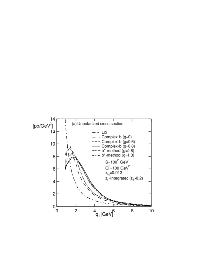
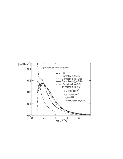
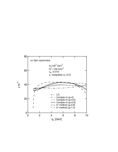
Figure 1: (a) Unpolarized SIDIS cross section for eRHIC kinematics. We show the fixed-order (LO) result, and resummed results for the complex-$b$ method with non-perturbative parameters $g=0$ and $g=0.6,\,0.8$ GeV², and for the $b^{\ast}$ method with $b_{\rm max}=1/(\sqrt{2}$ GeV$)$ and $g=0.8,\,1.3$ GeV². (b) Same for the longitudinally polarized case. (c) Spin asymmetries corresponding to the various cross sections shown in (a) and (b).

Figures 1 (a) and (b), respectively, show the unpolarized and polarized cross sections

$${1\over 2\pi}\int_{0.2}^{z_{f}^{max}}dz_{f}d\phi{d(\Delta)\sigma\over dx_{bj}dz_{f}dQ^{2}dq_{T}d\phi}$$ (57)

for eRHIC kinematics, where $z_{f}^{\rm max}$ is given in Eq. (A.6). Note that we have multiplied by a factor $q_{T}$, as compared to the cross section we considered in (19). The LO cross sections rapidly diverge as $q_{T}\to 0$. For the matched cross section using the complex-$b$ method with $g=0$, one obtains an enhancement at intermediate $q_{T}$ and the expected reduction at small $q_{T}$. The inclusion of the non-perturbative Gaussian form factor makes this tendency stronger. However, the results for different choices of the Gaussian, $g=0.6$ and $0.8$ GeV², are not very different and just have a slightly smaller normalization and are shifted to the right.

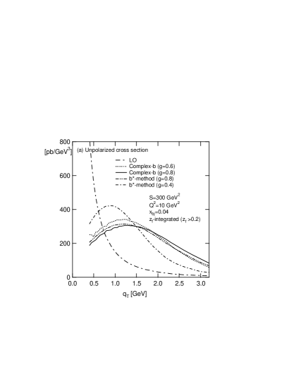
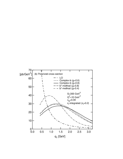
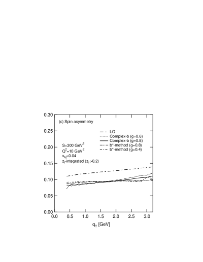
Figure 2: Same as in Figs. 1 (a)-(c), but for COMPASS kinematics. For the $b^{\ast}$ prescription, we have chosen here the non-perturbative parameters $g=0.4,\,0.8$ GeV².

Also shown in these figures are the curves for the $b^{\ast}$ prescription with $b_{\rm max}=1/(\sqrt{2}$ GeV$)$ and $g=0.8$ and $1.3$ GeV². For the eRHIC case, the choice of $g=0.8$ gives a result relatively close to the one with $g=0$ in the complex-$b$ method, while $g=1.3$ gives a result very close to those with $g=0.6$ and $0.8$ in the complex-$b$ method. One should note that these resummed curves all give a very similar $q_{T}$-integrated cross section, close to the full NLO one, due to our choice of $L$ in Eq. (46) and our matching procedure described in the previous subsection [51].

Figure 1 (c) shows the corresponding spin asymmetries, defined by the ratios of the polarized and unpolarized cross sections for all the curves shown in Figs. 1 (a) and (b). Although the effects of resummation and the non-perturbative Gaussians are significant in each cross section, they cancel to a large degree in the spin asymmetry. If one looks in more detail, resummation somewhat enhances the asymmetry compared to LO in the range of small to intermediate $q_{T}$, where also the cross sections shown in Figs. 1 (a) and (b) receive enhancements due to the resummation.

Figures 2 (a)-(c) show the same quantities as Figs.1 (a)-(c), now for the COMPASS kinematics described above. In this case, the complex-$b$ method without Gaussian smearing ($g=0$) turned out to be difficult to control numerically at small $q_{T}$, and we do not show the result for it. We find that resummation leads to a significant enhancement of the cross section at $q_{T}\geq 1$ GeV. In both unpolarized and polarized cross sections, the resummed results we show, for the complex-$b$ method with $g=0.6$ and $0.8$ GeV², and for the $b^{\ast}$ prescription with $b_{\rm max}=1/(\sqrt{2}$ GeV$)$ and $g=0.8$ GeV², turn out to be very similar, while the $b^{\ast}$ prescription with $g=0.4$ GeV² gives a higher peak that is shifted to the left compared to the other three resummed results. All these resummed results give a very similar spin asymmetry for the process $\vec{l}\vec{p}\to l\pi X$ for COMPASS kinematics; we find that resummation just leads to a moderate decrease of the asymmetry.

4 Summary and Conclusions

We have carried out a study of the soft-gluon resummation for the transverse-momentum ($q_{T}$) distribution in semi-inclusive deeply-inelastic scattering. Resummation is crucial at small transverse momenta, $q_{T}\ll Q$, where it takes into account large double-logarithmic corrections to all orders in the strong coupling constant. We have considered all relevant leading-twist double-spin cross sections, focusing on the terms that are independent of the angle between the lepton and the hadron planes, and have presented the resummation formulas for each.

We have performed phenomenological studies for the process $\vec{l}\vec{p}\to l\pi X$ at COMPASS and at a possible future polarized $ep$ collider, eRHIC. Here we have chosen two different prescriptions for treating the region of very large impact parameters in the Sudakov form factor, which is related to the onset of non-perturbative phenomena. We have used simple estimates for the non-perturbative term suggested by the resummed formula. Our results indicate that resummation effects as well as non-perturbative effects cancel to a large extent in the spin asymmetry.

Appendix A Analytic formulas for the LO cross sections

Here we summarize the LO cross section formulas for the processes in (1), which were derived in [10]. The differential cross sections are given by

$${d^{5}\sigma\over dx_{bj}dQ^{2}dz_{f}dq_{T}^{2}d\phi} = {\alpha_{em}^{2}\alpha_{s}\over 8\pi x_{bj}^{2}S_{ep}^{2}Q^{2}}\sum_{k}{\cal A}_{k}\int_{x_{min}}^{1}\,{dx\over x}\int_{z_{min}}^{1}\,{dz\over z}\,\left[f\circ D\circ\widehat{\sigma}_{k}\right]$$ (A.1)

$$\qquad\qquad\qquad\times\,\delta\left({q_{T}^{2}\over Q^{2}}-\left({1\over\widehat{x}}-1\right)\left({1\over\widehat{z}}-1\right)\right)\;,$$

where the ${\cal A}_{k}$ are defined as [10, 42]

$${\cal A}_{1} = 1+\cosh^{2}\psi\;,$$

$${\cal A}_{2} = -2\;,$$

$${\cal A}_{3} = -\cos\phi\sinh 2\psi\;,$$

$${\cal A}_{4} = \cos 2\phi\sinh^{2}\psi\;,$$

$${\cal A}_{6} = -2\cosh\psi\;,$$

$${\cal A}_{7} = 2\cos\phi\sinh\psi\;,$$

$${\cal A}_{8} = -\sin\phi\sinh 2\psi\;,$$

$${\cal A}_{9} = \sin 2\phi\sinh^{2}\psi\;,$$ (A.2)

and the summation over $k$ is $k=1,\ldots,4$ for processes (i) and (ii) in (1), $k=1,\ldots,4,8,9$ for process (iii), and $k=6,7$ for processes (iv) and (v) (see below). $\alpha_{em}=e^{2}/4\pi$ is the QED coupling constant, and we have introduced the variables

$$\widehat{x}={x_{bj}\over x}\;,\qquad\widehat{z}={z_{f}\over z}\;,$$ (A.3)

and

$$x_{min}=x_{bj}\left(1+{z_{f}\over 1-z_{f}}{q_{T}^{2}\over Q^{2}}\right)\;,\qquad z_{min}=z_{f}\left(1+{x_{bj}\over 1-x_{bj}}{q_{T}^{2}\over Q^{2}}\right)\;.$$ (A.4)

For a given $S_{ep}$, $Q^{2}$ and $q_{T}$, the kinematic constraints for $x_{bj}$ and $z_{f}$ are

$${Q^{2}\over S_{ep}}<x_{bj}<1\;,$$ (A.5)

$$0<z_{f}<{1-x_{bj}\over 1-x_{bj}+x_{bj}q_{T}^{2}/Q^{2}}\;.$$ (A.6)

Consequently, $q_{T}$ is limited by

$$0<q_{T}<Q\sqrt{\left({1\over x_{bj}}-1\right)\left({1\over z_{f}}-1\right)}\;.$$ (A.7)

In the hadron frame, the transverse momentum, $p_{T}$, of $p_{B}^{\mu}$ obeys

$$p_{T}=z_{f}q_{T}<z_{f}Q\sqrt{\left({1\over x_{bj}}-1\right)\left({1\over z_{f}}-1\right)}\;.$$ (A.8)

The term $\left[f\circ D\circ\widehat{\sigma}_{k}\right]$ in Eq. (A.1) takes the following form for the processes in (1):

(i) $e+p\rightarrow e+\pi+X$ [60]:

$$\left[f\circ D\circ\widehat{\sigma}_{k}\right] = \sum_{q,\bar{q}}e_{q}^{2}f_{q}(x)D_{q}(z)\widehat{\sigma}^{k}_{qq}+\sum_{q,\bar{q}}e_{q}^{2}f_{g}(x)D_{q}(z)\widehat{\sigma}^{k}_{qg}+\sum_{q,\bar{q}}e_{q}^{2}f_{q}(x)D_{g}(z)\widehat{\sigma}^{k}_{gq}\;,$$ (A.9)

where ($C_{F}=4/3$)

$$\widehat{\sigma}^{1}_{qq} = 2C_{F}\widehat{x}\widehat{z}\left\{{1\over Q^{2}q_{T}^{2}}\left({Q^{4}\over\widehat{x}^{2}\widehat{z}^{2}}+\left(Q^{2}-q_{T}^{2}\right)^{2}\right)+6\right\}\;,$$

$$\widehat{\sigma}^{2}_{qq} = 2\widehat{\sigma}_{4}^{qq}=8C_{F}\widehat{x}\widehat{z}\;,$$

$$\widehat{\sigma}^{3}_{qq} = 4C_{F}\widehat{x}\widehat{z}{1\over Qq_{T}}(Q^{2}+q_{T}^{2})\;,$$ (A.10)

$$\widehat{\sigma}^{1}_{qg} = \widehat{x}(1-\widehat{x})\left\{{Q^{2}\over q_{T}^{2}}\left({1\over\widehat{x}^{2}\widehat{z}^{2}}-{2\over\widehat{x}\widehat{z}}+2\right)+10-{2\over\widehat{x}}-{2\over\widehat{z}}\right\}\;,$$

$$\widehat{\sigma}^{2}_{qg} = 2\widehat{\sigma}^{4}_{qg}=8\widehat{x}(1-\widehat{x})\;,$$

$$\widehat{\sigma}^{3}_{qg} = \widehat{x}(1-\widehat{x}){2\over Qq_{T}}\left\{2(Q^{2}+q_{T}^{2})-{Q^{2}\over\widehat{x}\widehat{z}}\right\}\;,$$ (A.11)

$$\widehat{\sigma}^{1}_{gq} = 2C_{F}\widehat{x}(1-\widehat{z})\left\{{1\over Q^{2}q_{T}^{2}}\left({Q^{4}\over\widehat{x}^{2}\widehat{z}^{2}}+{(1-\widehat{z})^{2}\over\widehat{z}^{2}}\left(Q^{2}-{\widehat{z}^{2}q_{T}^{2}\over(1-\widehat{z})^{2}}\right)^{2}\right)+6\right\}\;,$$

$$\widehat{\sigma}^{2}_{gq} = 2\widehat{\sigma}^{4}_{gq}=8C_{F}\widehat{x}(1-\widehat{z})\;,$$

$$\widehat{\sigma}^{3}_{gq} = -4C_{F}\widehat{x}(1-\widehat{z})^{2}{1\over\widehat{z}Qq_{T}}\left\{Q^{2}+{\widehat{z}^{2}q_{T}^{2}\over(1-\widehat{z})^{2}}\right\}\;.$$ (A.12)

(ii) $e+\vec{p}\rightarrow e+\vec{\Lambda}+X$:

$$\left[f\circ D\circ\widehat{\sigma}_{k}\right] = \sum_{q,\bar{q}}e_{q}^{2}\Delta f_{q}(x)\Delta D_{q}(z)\Delta_{L}\widehat{\sigma}^{k}_{qq}+\sum_{q,\bar{q}}e_{q}^{2}\Delta f_{g}(x)\Delta D_{q}(z)\Delta_{L}\widehat{\sigma}^{k}_{qg}$$ (A.13)

$$\qquad\qquad+\sum_{q,\bar{q}}e_{q}^{2}\Delta f_{q}(x)\Delta D_{g}(z)\Delta_{L}\widehat{\sigma}^{k}_{gq}\;,$$

where

$$\Delta_{L}\widehat{\sigma}^{k}_{qq}=\widehat{\sigma}^{k}_{qq}\qquad(k=1,2,3,4)\;,$$ (A.14)

$$\Delta_{L}\widehat{\sigma}^{1}_{qg} = -{(2\widehat{x}-1)\left\{Q^{4}(\widehat{x}-1)^{2}-q_{T}^{4}\widehat{x}^{2}\right\}\over Q^{2}q_{T}^{2}\widehat{x}(\widehat{x}-1)}\;,$$

$$\Delta_{L}\widehat{\sigma}^{2}_{qg} = \Delta_{L}\widehat{\sigma}_{4}^{gq}=0\;,$$

$$\Delta_{L}\widehat{\sigma}^{3}_{qg} = -{2\left\{Q^{2}(\widehat{x}-1)-q_{T}^{2}\widehat{x}\right\}\over Qq_{T}}\;,$$ (A.15)

$$\Delta_{L}\widehat{\sigma}^{1}_{gq} = 2C_{F}\widehat{x}\widehat{z}\left\{{\widehat{x}-2\over\widehat{x}-1}+{\widehat{x}(\widehat{x}+1)\over(\widehat{x}-1)^{2}}{q_{T}^{4}\over Q^{4}}+{2(2\widehat{x}^{2}-2\widehat{x}+1)\over(\widehat{x}-1)^{2}}{q_{T}^{2}\over Q^{2}}\right\}\;,$$

$$\Delta_{L}\widehat{\sigma}^{2}_{gq} = 2\Delta_{L}\widehat{\sigma}_{4}^{qg}=8C_{F}{\widehat{x}^{2}\widehat{z}\over\widehat{x}-1}{q_{T}^{2}\over Q^{2}}\;,$$

$$\Delta_{L}\widehat{\sigma}^{3}_{gq} = {4C_{F}\widehat{x}\widehat{z}\over(\widehat{x}-1)^{2}}\left\{(\widehat{x}-1)^{2}+{\widehat{x}^{2}q_{T}^{2}\over Q^{2}}\right\}{q_{T}\over Q}\;.$$ (A.16)

(iii) $e+{p}^{\uparrow}\rightarrow e+{\Lambda}^{\uparrow}+X$:
For this process, it is more transparent to write the cross section by including the factors ${\cal A}_{k}$ in (A.1):

$$\sum_{k=1,\cdots,4,8,9}{\cal A}_{k}\left[f\circ D\circ\widehat{\sigma}_{k}\right]\equiv\sum_{q,\bar{q}}e_{q}^{2}\delta f_{q}(x)\delta D_{q}(z)\delta\widehat{\sigma}^{qq}\;,$$ (A.17)

where

$$\delta\widehat{\sigma}^{qq} = 4C_{F}\left[\left(1+\cosh^{2}\psi\right)\cos(\Phi_{A}-\Phi_{B})-{Q\over q_{T}}\sinh 2\psi\,\cos(\Phi_{A}-\Phi_{B}-\phi)\right.$$ (A.18)

$$\left.+{Q^{2}\over q_{T}^{2}}\sinh^{2}\psi\,\cos(\Phi_{A}-\Phi_{B}-2\phi)\right]\;.$$

Here the terms with ${\cal A}_{3}$ and ${\cal A}_{8}$ in Eq. (A.1) have been combined to give the $\cos(\Phi_{A}-\Phi_{B}-\phi)$ term in (A.18). Likewise, those with ${\cal A}_{4,9}$ give the term with $\cos(\Phi_{A}-\Phi_{B}-2\phi)$.

(iv) $\vec{e}+\vec{p}\rightarrow e+\pi+X$:

$$\left[f\circ D\circ\widehat{\sigma}_{k}\right] = \sum_{q,\bar{q}}e_{q}^{2}\Delta f_{q}(x)D_{q}(z)\Delta_{LO}\widehat{\sigma}^{k}_{qq}+\sum_{q,\bar{q}}e_{q}^{2}\Delta f_{g}(x)D_{q}(z)\Delta_{LO}\widehat{\sigma}^{k}_{qg}$$ (A.19)

$$\qquad\qquad+\sum_{q,\bar{q}}e_{q}^{2}\Delta f_{q}(x)D_{g}(z)\Delta_{LO}\widehat{\sigma}^{k}_{gq}\;,$$

where

$$\Delta_{LO}\widehat{\sigma}^{6}_{qq} = -2C_{F}\left\{\left({1\over\widehat{x}\widehat{z}}+\widehat{x}\widehat{z}\right){Q^{2}\over q_{T}^{2}}-{\widehat{x}\widehat{z}q_{T}^{2}\over Q^{2}}\right\}\;,$$

$$\Delta_{LO}\widehat{\sigma}^{7}_{qq} = -4C_{F}\widehat{x}\widehat{z}{Q^{2}-q_{T}^{2}\over Qq_{T}}\;,$$ (A.20)

$$\Delta_{LO}\widehat{\sigma}^{6}_{qg} = {2\widehat{x}-1\over\widehat{x}}\left(2\widehat{x}+{\widehat{x}-1\over\widehat{z}^{2}}{Q^{2}\over q_{T}^{2}}\right)\;,$$

$$\Delta_{LO}\widehat{\sigma}^{7}_{qg} = {2Q\over q_{T}}{(\widehat{x}-1)(2\widehat{z}-1)\over\widehat{z}}\;,$$ (A.21)

$$\Delta_{LO}\widehat{\sigma}^{6}_{gq} = {2C_{F}\widehat{z}\over\widehat{x}-1}\left\{{1\over\widehat{z}^{2}}-(\widehat{x}-1)^{2}+{\widehat{x}^{4}\over(\widehat{x}-1)^{2}}{q_{T}^{4}\over Q^{4}}\right\}\;,$$

$$\Delta_{LO}\widehat{\sigma}^{7}_{gq} = {4C_{F}\widehat{x}\widehat{z}\over\widehat{x}-1}\left(1-{\widehat{x}\over\widehat{z}}\right){q_{T}\over Q}\;.$$ (A.22)

(v) $\vec{e}+{p}\rightarrow e+\vec{\Lambda}+X$:

$$\left[f\circ D\circ\widehat{\sigma}_{k}\right] = \sum_{q,\bar{q}}e_{q}^{2}f_{q}(x)\Delta D_{q}(z)\Delta_{OL}\widehat{\sigma}^{k}_{qq}+\sum_{q,\bar{q}}e_{q}^{2}f_{g}(x)\Delta D_{q}(z)\Delta_{OL}\widehat{\sigma}^{k}_{qg}$$ (A.23)

$$\qquad\qquad+\sum_{q,\bar{q}}e_{q}^{2}f_{q}(x)\Delta D_{g}(z)\Delta_{OL}\widehat{\sigma}^{k}_{gq}\;,$$

where

$$\Delta_{OL}\widehat{\sigma}^{6,7}_{qq}=\Delta_{LO}\widehat{\sigma}^{6,7}_{qq}\;,$$ (A.24)

$$\Delta_{OL}\widehat{\sigma}^{6}_{qg} = {2\widehat{x}^{2}-2\widehat{x}+1\over\widehat{x}\widehat{z}}\left(\widehat{x}+(\widehat{x}-1){Q^{2}\over q_{T}^{2}}\right)\;,$$

$$\Delta_{OL}\widehat{\sigma}^{7}_{qg} = {2Q\over q_{T}}{(\widehat{x}-1)(2\widehat{x}-1)\over\widehat{z}}\;,$$ (A.25)

$$\Delta_{OL}\widehat{\sigma}^{6}_{gq} = {2C_{F}\widehat{z}\over\widehat{x}-1}\left\{{1\over\widehat{z}^{2}}+(\widehat{x}-1)^{2}-{\widehat{x}^{4}\over(\widehat{x}-1)^{2}}{q_{T}^{4}\over Q^{4}}\right\}\;,$$

$$\Delta_{OL}\widehat{\sigma}^{7}_{gq} = -{4C_{F}\widehat{x}\widehat{z}\over\widehat{x}-1}\left(1-{\widehat{x}\over\widehat{z}}\right){q_{T}\over Q}\;.$$ (A.26)

References

• [1] A. Airapetian et al. [HERMES Collaboration], Phys. Rev. Lett.  92 (2004) 012005 [arXiv:hep-ex/0307064]; Phys. Rev. D 71 (2005) 012003 [arXiv:hep-ex/0407032];
S. Platchkov [COMPASS Collaboration], talk given at the “Particles and Nuclei International Conference (PANIC05)”, Santa Fe, New Mexico, October 2005;
for earlier data, see: B. Adeva et al. [Spin Muon Collaboration], Phys. Lett. B 420 (1998) 180 [arXiv:hep-ex/9711008].
• [2] for reviews, see: M. Anselmino, A. Efremov and E. Leader, Phys. Rept.  261 (1995) 1 [Erratum-ibid.  281 (1997) 399];
V. Barone, A. Drago and P. G. Ratcliffe, Phys. Rept.  359 (2002) 1;
S. D. Bass, Rev. Mod. Phys.  77 (2005) 1257 [arXiv:hep-ph/0411005].
• [3] A. Airapetian et al. [HERMES Collaboration], Phys. Rev. Lett.  94 (2005) 012002 [arXiv:hep-ex/0408013];
M. Diefenthaler [HERMES Collaboration], AIP Conf. Proc.  792 (2005) 933 [arXiv:hep-ex/0507013].
• [4] V. Y. Alexakhin et al. [COMPASS Collaboration], Phys. Rev. Lett.  94 (2005) 202002 (2005) [arXiv:hep-ex/0503002].
• [5] D. Adams et al. [Spin Muon Collaboration (SMC)], Phys. Lett. B 336 (1994) 125 (1994);
A. Bravar [Spin Muon Collaboration], Nucl. Phys. A 666 (2000) 314.
• [6] H. Avakian [CLAS Collaboration], talk presented at the RBRC workshop “Single-Spin Asymmetries”, Brookhaven National Laboratory, Upton, New York, June 1-3, 2005.
• [7] D. W. Sivers, Phys. Rev. D 41 (1990) 83; Phys. Rev. D 43 (1991) 261.
• [8] J. C. Collins, Nucl. Phys. B 396 (1993) 161 [arXiv:hep-ph/9208213].
• [9] A. Deshpande, R. Milner, R. Venugopalan and W. Vogelsang, Ann. Rev. Nucl. Part. Sci.  55 (2005) 165 [arXiv:hep-ph/0506148].
• [10] Y. Koike and J. Nagashima, Nucl. Phys. B 660 (2003) 269 [arXiv:hep-ph/0302061].
• [11] P. Aurenche, R. Basu, M. Fontannaz and R. M. Godbole, Eur. Phys. J. C 34 (2004) 277 [arXiv:hep-ph/0312359].
• [12] A. Daleo, D. de Florian and R. Sassot, Phys. Rev. D 71 (2005) 034013 [arXiv:hep-ph/0411212].
• [13] B. A. Kniehl, G. Kramer and M. Maniatis, Nucl. Phys. B 711 (2005) 345 [Erratum-ibid. B 720 (2005) 231] [arXiv:hep-ph/0411300].
• [14] F. E. Close and R. G. Milner, Phys. Rev. D 44 (1991) 3691;
L. L. Frankfurt et al., Phys. Lett. B 230 (1989) 141;
X. D. Ji, Phys. Rev. D 49 (1994) 114 [arXiv:hep-ph/9307235].
• [15] D. de Florian, C.A. Garcia Canal and R. Sassot, Nucl. Phys. B 470 (1996) 195 [arXiv:hep-ph/9510262];
D. de Florian and R. Sassot, Nucl. Phys. B 488 (1997) 367 [arXiv:hep-ph/9610362].
• [16] D. de Florian, M. Stratmann and W. Vogelsang, Phys. Rev. D 57 (1998) 5811 [arXiv:hep-ph/9711387].
• [17] A. Daleo, C. A. Garcia Canal and R. Sassot, Nucl. Phys. B 662 (2003) 334 [arXiv:hep-ph/0303199];
A. Daleo and R. Sassot, Nucl. Phys. B 673 (2003) 357 [arXiv:hep-ph/0309073].
• [18] Y. L. Dokshitzer, D. Diakonov and S. I. Troian, Phys. Lett. B 79 (1978) 269.
• [19] G. Parisi and R. Petronzio, Nucl. Phys. B 154 (1979) 427.
• [20] J. C. Collins and D. E. Soper, Nucl. Phys. B 193 (1981) 381 [Erratum-ibid. B 213 (1983) 545]; Nucl. Phys. B 197 (1982) 446.
• [21] G. Altarelli, R. K. Ellis, M. Greco and G. Martinelli, Nucl. Phys. B 246 (1984) 12.
• [22] J. C. Collins, D. E. Soper and G. Sterman, Nucl. Phys. B 250 (1985) 199.
• [23] R. Meng, F. I. Olness and D. E. Soper, Phys. Rev. D 54 (1996) 1919 [arXiv:hep-ph/9511311].
• [24] P. Nadolsky, D. R. Stump and C. P. Yuan, Phys. Rev. D 61 (2000) 014003 [Erratum-ibid. D 64 (2001) 059903] [arXiv:hep-ph/9906280]; Phys. Rev. D 64 (2001) 114011 [arXiv:hep-ph/0012261]; Phys. Lett. B 515 (2001) 175 [arXiv:hep-ph/0012262].
• [25] I. Abt et al. [H1 Collaboration], Z. Phys. C 63 (1994) 377;
S. Aid et al. [H1 Collaboration], Z. Phys. C 70 (1996) 609 [arXiv:hep-ex/9602001]; S. Aid et al. [H1 Collaboration], Z. Phys. C 72 (1996) 573 [arXiv:hep-ex/9608011];
I. Abt et al. [H1 Collaboration], Phys. Lett. B 328 (1994) 176;
C. Adloff et al. [H1 Collaboration], Nucl. Phys. B 485 (1997) 3 [arXiv:hep-ex/9610006];
S. Aid et al. [H1 Collaboration], Phys. Lett. B 356 (1995) 118 [arXiv:hep-ex/9506012];
C. Adloff et al. [H1 Collaboration], Eur. Phys. J. C 12 (2000) 595 [arXiv:hep-ex/9907027].
• [26] M. Derrick et al. [ZEUS Collaboration], Z. Phys. C 70 (1996) 1 [arXiv:hep-ex/9511010];
J. Breitweg et al. [ZEUS Collaboration], Phys. Lett. B 481 (2000) 199 [arXiv:hep-ex/0003017].
• [27] A. Weber, Nucl. Phys. B 382 (1992) 63; Nucl. Phys. B 403 (1993) 545.
• [28] H. Kawamura, J. Kodaira, H. Shimizu and K. Tanaka, arXiv:hep-ph/0512137.
• [29] A. Weber, DO-TH-92-28 (Thesis, Dortmund University, unpublished).
• [30] D. Boer, Phys. Rev. D 62 (2000) 094029 [arXiv:hep-ph/0004217].
• [31] D. Boer, Nucl. Phys. B 603 (2001) 195 [arXiv:hep-ph/0102071].
• [32] A. Idilbi, X. D. Ji, J. P. Ma and F. Yuan, Phys. Rev. D 70 (2004) 074021 [arXiv:hep-ph/0406302].
• [33] X. D. Ji, J. P. Ma and F. Yuan, Phys. Lett. B 597 (2004) 299 [arXiv:hep-ph/0405085].
• [34] C. T. H. Davies and W. J. Stirling, Nucl. Phys. B 244 (1984) 337.
• [35] C. T. H. Davies, B. R. Webber and W. J. Stirling, Nucl. Phys. B 256 (1985) 413;
P. B. Arnold and R. P. Kauffman, Nucl. Phys. B 349 (1991) 381;
G. A. Ladinsky and C. P. Yuan, Phys. Rev. D 50 (1994) 4239 [arXiv:hep-ph/9311341];
F. Landry, R. Brock, G. Ladinsky and C. P. Yuan, Phys. Rev. D 63 (2001) 013004 [arXiv:hep-ph/9905391];
F. Landry, R. Brock, P. M. Nadolsky and C. P. Yuan, Phys. Rev. D 67 (2003) 073016 [arXiv:hep-ph/0212159];
C. Balazs and C. P. Yuan, Phys. Rev. D 56 (1997) 5558 [arXiv:hep-ph/9704258].
• [36] A. V. Konychev and P. M. Nadolsky, arXiv:hep-ph/0506225.
• [37] A. Kulesza, G. Sterman and W. Vogelsang, Phys. Rev. D 66 (2002) 014011 [arXiv:hep-ph/0202251].
• [38] J. W. Qiu and X. F. Zhang, Phys. Rev. D 63 (2001) 114011 [arXiv:hep-ph/0012348].
• [39] for further discussion, see also: S. Tafat, JHEP 0105 (2001) 004 [arXiv:hep-ph/0102237].
• [40] X. D. Ji, J. W. Qiu, W. Vogelsang and F. Yuan, in preparation.
• [41] D. Boer and W. Vogelsang, in preparation.
• [42] R. Meng, F. Olness and D. Soper, Nucl. Phys. B 371 (1992) 79.
• [43] for a clear discussion, see also: P. M. Nadolsky, arXiv:hep-ph/0108099.
• [44] J. Kodaira and L. Trentadue, Phys. Lett. B 112 (1982) 66; Phys. Lett. B 123 (1983) 335.
• [45] D. de Florian and M. Grazzini, Phys. Rev. Lett.  85 (2000) 4678 [arXiv:hep-ph/0008152]; Nucl. Phys. B 616 (2001) 247 [arXiv:hep-ph/0108273].
• [46] R. K. Ellis, D. A. Ross and A. E. Terrano, Nucl. Phys. B 178 (1981) 421.
• [47] W. Vogelsang, Nucl. Phys. B 475 (1996) 47 [arXiv:hep-ph/9603366].
• [48] W. Vogelsang, Phys. Rev. D 57 (1998) 1886 [arXiv:hep-ph/9706511].
• [49] M. Stratmann and W. Vogelsang, Nucl. Phys. B 496 (1997) 41 [arXiv:hep-ph/9612250].
• [50] S. Frixione, P. Nason and G. Ridolfi, Nucl. Phys. B 542 (1999) 311 [arXiv:hep-ph/9809367].
• [51] G. Bozzi, S. Catani, D. de Florian and M. Grazzini, Nucl. Phys. B 737 (2006) 73 [arXiv:hep-ph/0508068].
• [52] see: G. Sterman and W. Vogelsang, Phys. Rev. D 71 (2005) 014013 [arXiv:hep-ph/0409234], and references therein.
• [53] S. Berge, P. Nadolsky, F. Olness and C. P. Yuan, Phys. Rev. D 72 (2005) 033015 [arXiv:hep-ph/0410375].
• [54] E. Laenen, G. Sterman and W. Vogelsang, Phys. Rev. Lett.  84 (2000) 4296 [arXiv:hep-ph/0002078]; Phys. Rev. D 63 (2001) 114018 [arXiv:hep-ph/0010080].
• [55] A. Kulesza, G. Sterman and W. Vogelsang, Phys. Rev. D 69 (2004) 014012 [arXiv:hep-ph/0309264].
• [56] R. K. Ellis and S. Veseli, Nucl. Phys. B 511 (1998) 649 [arXiv:hep-ph/9706526];
A. Kulesza and W. J. Stirling, Nucl. Phys. B 555 (1999) 279 [arXiv:hep-ph/9902234]; JHEP 0001 (2000) 016 [arXiv:hep-ph/9909271]; Eur. Phys. J. C 20 (2001) 349 [arXiv:hep-ph/0103089].
• [57] M. Glück, E. Reya and A. Vogt, Eur. Phys. J. C 5 (1998) 461 [arXiv:hep-ph/9806404].
• [58] M. Glück, E. Reya, M. Stratmann and W. Vogelsang, Phys. Rev. D 63 (2001) 094005 [arXiv:hep-ph/0011215].
• [59] S. Kretzer, Phys. Rev. D 62 (2000) 054001 [arXiv:hep-ph/0003177].
• [60] A. Mendez, Nucl. Phys. B 145 (1978) 199.