Stable gapless superconductivity at strong coupling

Abstract

We study cross-flavor Cooper pairing in a relativistic system of two fermion species with mismatched Fermi surfaces. We find that there exist gapless phases which are characterized by either one or two gapless nodes in the energy spectra of their quasiparticles. An analysis of the current-current correlator reveals that, at strong coupling, both of these gapless phases can be free of magnetic instabilities and thus are stable. This is in contrast to the weak-coupling case where there are always two gapless nodes and the phase becomes magnetically unstable.

I Introduction

In recent years, the interest in degenerate fermionic systems has considerably increased. In part, this was driven by a substantial progress in experimental studies of trapped cold gases of fermionic atoms cold-atoms . By making use of various techniques, it has become possible to prepare atomic systems of different composition, temperature, density, and coupling strength of the interaction. Because of such a flexibility, the basic knowledge gained in these studies is likely to be of immense value also outside the realm of atomic physics. For example, the knowledge of the ground state of an asymmetric mixture of two atomic species can shed light on the physical properties of strongly interacting dense quark matter that may exist in stars.

It is conjectured that the baryon density in the central regions of compact (neutron) stars is sufficiently high for crushing nucleons (and strange baryons if there are any) into deconfined quark matter. The ground state of such matter is expected to be a color superconductor old ; sc . (For reviews on color superconductivity, see Ref. reviews .) At high density the energetically preferred phase is the so-called color-flavor-locked (CFL) phase CFL . At densities of relevance for compact stars, however, the situation is much less clear.

The difficulties in predicting the ground state of dense quark matter are related to the fact that the conditions of charge neutrality and $\beta$ equilibrium in a macroscopic bulk of matter such as the core of a compact star have a disruptive effect on quark Cooper pairing no2sc ; no2sc-other . For example, as emphasized in Ref. SH03 , enforcing charge neutrality can result in unconventional forms of superconductivity, such as the gapless 2-flavor color-superconducting (g2SC) phase. A 3-flavor version, the so-called gapless color-flavor-locked phase (gCFL), was also proposed gCFL . While it was argued that both types of gapless phases are (chromo-)magnetically unstable HS04 ; instability-CFL ; Fuku05 (for the non-relativistic case, see Ref. WuYip ), there exist convincing arguments that unconventional Cooper pairing in one form or another is unavoidable RajSch . By taking into account the general observation of Refs. pd1 ; pd2 ; pd3 ; pd4 ; pd5 that the role of gapless phases diminishes with increasing coupling strength, one may naively conclude that gapless phases do not exist in the regime of strong coupling. In this paper, we show that this conclusion is premature: not only do such phases exist, but they can even be magnetically stable.

Since the QCD coupling becomes strong at low densities, one may conjecture that quark matter undergoes Bose-Einstein condensation (BEC) of diquarks rather than forming the usual Cooper pairs of the Bardeen-Cooper-Schrieffer (BCS) type CSC-BEC ; KKKN04 ; NA05 ; NNY05 . If this is indeed the case, one may observe well-pronounced diquark-pair fluctuations in the vicinity of the critical temperature KKKN02 ; Vosk04 ; JZ05 and/or the formation of a pseudogap phase KKKN04 . Therefore, it is of interest to study Cooper pairing in the strongly coupled regime in more detail.

In this paper, we address the issue of the existence of stable gapless phases in a strongly coupled system of two species of massive fermions. (For a related study, based on an effective low-energy description, see also Ref. SS05 ). To keep the discussion as simple and as general as possible, we consider a model with a local interaction that describes two fermion species with equal masses, but with non-equal chemical potentials. We find that gapless phases with either one or two effective Fermi surfaces can exist at strong coupling. These phases are stable in the sense that they are free of (chromo-)magnetic instabilities HS04 . It is expected that many results of our analysis should remain qualitatively similar also in the more complicated case of non-equal masses.

The paper is organized as follows. In the next section, we briefly introduce the model and set up the notation. In Sec. III, we present the zero-temperature phase diagram in the plane of the average chemical potential and the coupling constant for several values of the mismatch between the fermion chemical potentials. This diagram, while obtained in the mean-field (MF) approximation and, thus, not completely reliable at strong coupling, reveals a very interesting feature: it has regions of gapless phases that are free of the Sarma instability Sarma without imposing the neutrality condition. Note that this is drastically different from the situation at weak coupling, where the absence of such an instability is mainly due to charge neutrality SH03 ; gCFL , or other types of constraints on the system bp . In Sec. IV, we calculate the screening masses, defined by the long-wavelength limit of the static particle-number current-current correlator, and reveal a region of parameters (generally at strong coupling) for which gapless superconductivity is stable. The discussion of the results and conclusions are given in Sec. V.

II Model and quasiparticle spectrum

Let us start by introducing the Lagrangian density of the model,

$${\cal L}=\bar{\psi}(i\not{\partial}-m+\hat{\mu}\gamma^{0})\psi+{\cal L}_{I},$$ (1)

where $\psi$ denotes the Dirac field which has two internal degrees of freedom, called “flavors” in the following. In general, the mass is a diagonal matrix of the form $\hat{m}={\rm diag}(m_{1},m_{2})$. For simplicity, however, we restrict ourselves to the case of equal fermion masses, i.e., we use $m_{1}=m_{2}=m$ in this paper. No constraints on the values of the chemical potentials of the two flavors of fermions are imposed, i.e., $\hat{\mu}={\rm diag}(\mu_{1},\mu_{2})$ where $\mu_{1}$ and $\mu_{2}$ need not be equal.

In order to study superfluidity/superconductivity that results from Cooper pairing of different flavors of fermions, we introduce the following local interaction term to the Lagrangian density,

$${\cal L}_{I}=G(\bar{\psi}i\gamma_{5}\sigma_{1}C\bar{\psi}^{T})(\psi^{T}i\gamma_{5}\sigma_{1}C\psi),$$ (2)

where $G$ is the coupling constant, $\sigma_{1}$ is the (symmetric) Pauli matrix in flavor space, and $C=i\gamma_{0}\gamma_{2}$ is the charge conjugation matrix. This term describes a cross-flavor attractive interaction between fermions that can drive the formation of spin-zero (and, therefore, totally antisymmetric) Cooper pairs at weak coupling, or even cause the appearance of localized bound states at strong coupling. At sufficiently low temperature, these bosonic states should form a condensate in the ground state. The explicit structure of the condensate is given by the following expression,

$$\Delta=2G\langle\psi^{T}Ci\gamma_{5}\sigma_{1}\psi\rangle.$$ (3)

In the MF approximation, the value of $\Delta$ is determined by the minimization of the effective potential

$$V(\Delta)=\frac{\Delta^{2}}{4G}-\frac{T}{2}\sum_{n}\int\frac{d^{3}k}{(2\pi)^{3}}{\rm Tr}\log[S^{-1}(K)],$$ (4)

where $S^{-1}(K)$ is the inverse fermion propagator in Nambu-Gor’kov space,

$$[S(K)]^{-1}=\left(\begin{array}[]{cc}\not{K}+\hat{\mu}\gamma^{0}-\hat{m}&-i\sigma_{1}\gamma_{5}\Delta\\ -i\sigma_{1}\gamma_{5}\Delta&\not{K}-\hat{\mu}\gamma^{0}-\hat{m}\end{array}\right).$$ (7)

The corresponding Nambu-Gor’kov spinor is defined by $\Psi^{T}=(\psi^{T},\psi_{C}^{T})$ with $\psi_{C}\equiv C{\bar{\psi}}^{T}$ being the charge-conjugate spinor.

The (eight) poles of the determinant $\mbox{det}\left[S(K)\right]$ determine the dispersion relations of (eight) quasiparticles. In the case of equal fermion masses, these can be given explicitly in analytical form,

$$k_{0}=\pm\left(\epsilon_{\pm}\pm\delta\mu\right),$$ (8)

where all eight sign combinations are possible. In the above equation, we used the following notation:

$$\epsilon_{\pm} = \sqrt{(E_{k}\pm\bar{\mu})^{2}+\Delta^{2}},$$ (9)

$$E_{k} = \sqrt{k^{2}+m^{2}},$$ (10)

$$\bar{\mu} = \frac{\mu_{1}+\mu_{2}}{2},$$ (11)

$$\delta\mu = \frac{\mu_{1}-\mu_{2}}{2}$$ (12)

(without loss of generality, we assume that $\bar{\mu}\geq 0$ and $\delta\mu\geq 0$).

Let us first clarify the structure of the quasiparticle excitation spectrum keeping $\Delta/\delta\mu$ and $\bar{\mu}/m$ as free parameters, i.e., without actually solving a gap equation. It is easy to see that, if $\Delta/\delta\mu>1$, there are no gapless excitations irrespective of the value of $\bar{\mu}/m$. This is not always the case when $\Delta/\delta\mu\leq 1$, cf. Ref. SH03 . In this case, gapless modes may exist around effective Fermi surfaces at momenta

$$k_{\pm}=\sqrt{\left(\bar{\mu}\pm\sqrt{\delta\mu^{2}-\Delta^{2}}\right)^{2}-m^{2}}.$$ (13)

Of course, $k_{\pm}$ has to be real, otherwise the corresponding effective Fermi surface does not exist. If $\bar{\mu}/m$ is sufficiently large, both $k_{+}$ and $k_{-}$ are real, and there are two effective Fermi surfaces. For $\Delta\neq 0$, we call the corresponding gapless superconducting phase the gSC(2) phase. Such gapless phases were discussed in the context of dense quark matter SH03 ; gCFL ; pd1 ; pd2 ; pd3 ; pd4 ; pd5 . A typical excitation spectrum is depicted in Fig. 1(a). For smaller values of $\bar{\mu}/m$, $k_{-}$ has a non-zero imaginary part while $k_{+}$ is real, and there is only one effective Fermi surface, cf. Fig. 1(b). We call the corresponding gapless superconducting phase the gSC(1) phase. Finally, for even smaller values of $\bar{\mu}/m$, both $k_{-}$ and $k_{+}$ have non-zero imaginary parts, and there are no gapless excitations in the spectrum; we are in a regular, gapped superconducting (SC) phase, cf. Fig. 1(c), just as in the case $\Delta/\delta\mu>1$, cf. Fig. 1(d).

Figure 1: Typical quasiparticle excitation spectra in gapless and regular superconducting phases. The values of $\bar{\mu}/m$ and $\Delta/\delta\mu$ are specified inside the panels. In all four cases $\delta\mu/m=0.5$. Excitation spectra of antiparticles are not shown.

In Fig. 2, we show where the three different types of superconducting phases occur in the plane of $\Delta/\delta\mu$ and $\bar{\mu}/m$, for a fixed value of $\delta\mu/m=0.5$. The boundary of the region gSC(1) can be derived from the requirement that $k_{-}=0$, i.e., the region exists for values of $\Delta/\delta\mu$ and $\bar{\mu}/m$ satisfying the condition

$$\left(\frac{\Delta}{\delta\mu}\right)^{2}+\left(\frac{\bar{\mu}-m}{\delta\mu}\right)^{2}\leq 1.$$ (14)

The boundary between the gSC(2) and SC regions is given by $\Delta/\delta\mu=1$ for $\bar{\mu}/m\geq 1$. The three regions SC, gSC(1) and gSC(2) meet at the “splitting” point S, cf. Ref. SS05 .

Figure 2: The phase diagram in the plane of $\Delta/\delta\mu$ and $\bar{\mu}/m$ plotted for a fixed value of $\delta\mu/m=0.5$. The region SC represents a superconducting phase without gapless modes, while gSC(1) and gSC(2) represent phases with one and two effective Fermi surfaces, respectively. The three regions merge at the splitting point “S”, cf. Ref. SS05 . For a given $m/\Lambda$, the region to the right of the dashed line (from top to bottom, $m/\Lambda=0.3$, $0.2$, and $0.1$) is not accessible in the MF analysis of Fig. 3, see text for a detailed explanation. For $m/\Lambda=0.2$, the “screening mass” $m_{M}$ is imaginary in the shaded area.

III Phase diagram

In this section, we explore the phase diagram of the model at hand in the plane of the average chemical potential $\bar{\mu}$ and the coupling constant $G$. We shall restrict our study to the zero-temperature case when the problems with the stability of gapless phases are expected to be most prominent. Then, the effective potential reads

$$V(\Delta) = \frac{\Delta^{2}}{4G}-\int_{0}^{\Lambda}\frac{k^{2}dk}{2\pi^{2}}\Big{(}|\epsilon_{-}+\delta\mu|+|\epsilon_{-}-\delta\mu|$$ (15)

$$+|\epsilon_{+}+\delta\mu|+|\epsilon_{+}-\delta\mu|\Big{)},$$

where $\Lambda$ is a momentum cut-off.

In Fig. 3, we show the phase diagram for three different values of the fermion masses, $m/\Lambda=0.1$, $0.2$ and $0.3$, and a fixed value of $\delta\mu/m=0.5$. The coupling constant is normalized by $G_{0}=4\pi/\Lambda^{2}$. Note that, for $m=0$ and for $G\geq G_{0}$, the vacuum is unstable with respect to BEC of diquarks. The bold and thin solid lines represent first- and second-order transitions, respectively. For each choice of mass, the part of the diagram above the transition lines corresponds to the fully gapped superconducting phase. The small regions bounded by the solid and dotted lines in the middle of the phase diagram correspond to gapless phases. Below the solid lines, the system is in the normal phase. The normal phase to the left of the thin dashed vertical lines at $\bar{\mu}=m-\delta\mu$ corresponds to the vacuum.

Figure 3: The phase diagram in the plane of $G/G_{0}$ and $\bar{\mu}/\Lambda$ for three different values of the fermion masses, $m/\Lambda=0.1$, $0.2$ and $0.3$, and a fixed value of $\delta\mu/m=0.5$. The bold and thin lines represent first- and second-order transitions, respectively. The insertion is an enlarged view of the endpoint of the first-order transition line in the case of $m/\Lambda=0.1$.

As one can see from Fig. 3, at weak coupling the phase transition between the normal and superconducting phase is of first order. This is quite natural when there is a fixed mismatch between the chemical potentials of pairing fermions. With increasing the coupling constant $G$, the critical chemical potential $\bar{\mu}$ becomes smaller and the lines of first-order phase transitions terminate at endpoints. It is worth mentioning that the endpoints lie completely inside the region of the superconducting phase when $m/\Lambda=0.1$ and $0.2$. In the case $m/\Lambda=0.1$, one can see this more clearly from the insertion in the lower left corner of Fig. 3. In the case $m/\Lambda=0.3$, however, the corresponding endpoint lies on the phase boundary between normal and superconducting matter, or so close to it that our numerical resolution is not sufficient to make a distinction.

Across the boundary of a second-order phase transition, the gap $\Delta$ must be continuous. This means that the gap assumes arbitrarily small values just above the thin solid lines in Fig. 3. When the mismatch between the chemical potentials $\delta\mu$ is non-zero, there inevitably exists a region adjacent to the transition line where $\Delta<\delta\mu$. From Fig. 2 we see that this is a necessary condition to have a gapless phase, and this is precisely what we observe in Fig. 3. It is, however, not a sufficient condition: if $\bar{\mu}/\Lambda$ is sufficiently small, we could also have a gapped phase, as seen to the left of the gSC(1) region in Fig. 2.

The gapless phases in Fig. 3 correspond to global minima of the effective potential and, thus, they are free of the Sarma instability Sarma . This might be surprising since we do not impose additional constraints such as neutrality. An apparent discrepancy between this finding and that of Ref. SH03 is resolved by noting that the stable gapless phases in Fig. 3 always occur at strong coupling.

We now want to clarify which regions in Fig. 2 are accessible by the MF calculation that gives rise to the phase diagram in Fig. 3. We first note that the region below the solid lines in Fig. 3 represents the vacuum or the normal-conducting phase. Since there $\Delta=0$, moving along its upper boundary corresponds to moving along the horizontal axis in Fig. 2. Across a first-order phase transition, the gap is discontinuous. Therefore, certain values of $\Delta/\delta\mu$ are excluded. These can be found by computing the values of the gap along both sides of the bold solid lines in Fig. 3. For fixed $m/\Lambda$, such a path starts at the merging point of the second- and first-order transition lines in Fig. 3, continues along the lower side of the bold line, and runs around the endpoint, before continuing along the upper side of the first-order transition line. In Fig. 2, this path is shown as a dashed line. The region to the right of this line is not accessible in the MF analysis. As a consequence, the only gapless phases appearing in the phase diagram in Fig. 3 are those of type gSC(1). This excludes, therefore, possible ground states that correspond to the gSC(2) region as well as the splitting point S. In fact, the statement regarding the splitting point can be made rigorous by noting that the second derivative of the effective potential $\partial^{2}V/\partial\Delta^{2}$ is negative at S, meaning that this point cannot be a minimum of $V(\Delta)$. Of course, this conclusion may easily change if an additional constraint (e.g., such as neutrality) is imposed on the system.

Now, it is natural to ask whether the gSC(1) and gSC(2) types of gapless phases are subject to the chromomagnetic instability HS04 . This is studied in detail in the next section.

IV Stability Analysis

In this section, we discuss the stability of the gapless phases that were introduced in Sec. II, see Fig. 2. To this end, we calculate the fermion-number current-current correlator and study when such a correlator points toward an instability. Note that the use of the fermion-number current is not accidental here. When the vacuum expectation value in Eq. (3) is non-zero, the fermion-number symmetry is spontaneously broken.

By definition, the current-current correlator is given by

$$\Pi^{\mu\nu}(P)=\frac{T}{2}\sum_{n}\int\frac{d^{3}{\mathbf{k}}}{(2\pi)^{3}}{\rm Tr}\left[\hat{\Gamma}^{\mu}{\cal S}(K)\hat{\Gamma}^{\nu}{\cal S}(K-P)\right],$$ (16)

where $\hat{\Gamma}^{\mu}\equiv\mbox{diag}(i\gamma^{\mu},-i\gamma^{\mu})$ is the vertex in Nambu-Gor’kov space. Following the approach of Ref. HS04 , we consider $\Pi^{\mu\nu}$ only in the static ($p_{0}=0$) and long wave-length limit ($p\to 0$). Then, it is convenient to introduce the “screening masses” which are defined by

$$m_{D}^{2} = -\lim_{{\bf p}\to 0}\Pi^{00}(\omega=0,{\bf p}),$$ (17)

$$m_{M}^{2} = -\frac{1}{2}\lim_{{\bf p}\to 0}(g_{ij}+\hat{\bf p}_{i}\hat{\bf p}_{j})\Pi^{ij}(\omega=0,{\bf p}).$$ (18)

If the fermion-number symmetry is promoted to a gauge symmetry, the quantities $m_{D}$ and $m_{M}$ would describe the electric and magnetic screening properties of a superconductor.

Our calculations show that $m_{D}^{2}$ is positive definite in the whole of plane of $\Delta/\delta\mu$ and $\bar{\mu}/m$, see Fig. 2. However, the magnetic screening mass $m_{M}$ could be imaginary (i.e., $m_{M}^{2}<0$) in some cases when $\delta\mu$ is nonzero. In general, an imaginary result for $m_{M}$ indicates an instability with respect to the formation of inhomogeneities in the system RR ; GR05 . In the weak-coupling limit, the instabilities develop when $\Delta<\delta\mu$ HS04 . In this paper, we study whether a similar instability also develops at strong coupling.

When $\Delta$ is nonzero, the Nambu-Gor’kov propagator of fermions has both diagonal and off-diagonal components, see Eq. (7). Their contributions to the current-current correlator (16) can be considered separately. Then, the expression for $m_{M}^{2}$ can be given in the following form:

$$m_{M}^{2}=(m_{M}^{2})_{\rm diag}+(m_{M}^{2})_{\rm off}.$$ (19)

Each of the two types of contributions in this equation can be further subdivided into particle-particle (pp), antiparticle-antiparticle (aa), and particle-antiparticle (pa) parts, i.e.,

$$(m_{M}^{2})_{\rm diag}=(m_{M}^{2})_{\rm diag}^{\rm(pp)}+(m_{M}^{2})_{\rm diag}^{\rm(aa)}+(m_{M}^{2})_{\rm diag}^{\rm(pa)},$$ (20)

and a similar representation holds for $(m_{M}^{2})_{\rm off}$. The explicit expressions for all contributions are given by

$$(m_{M}^{2})_{\rm diag}^{\rm(pp),(aa)} = \frac{1}{3}\int\frac{d^{3}k}{(2\pi)^{3}}\frac{k^{2}}{E_{k}^{2}}\left(-\frac{\Delta^{2}}{\epsilon_{\mp}^{3}}\left[1-\theta(-\epsilon_{\mp}+\delta\mu)\right]-\frac{\epsilon_{\mp}^{2}+E_{\mp}^{2}}{\epsilon_{\mp}^{2}}\delta(\epsilon_{\mp}-\delta\mu)\right),$$ (21)

$$(m_{M}^{2})_{\rm off}^{\rm(pp),(aa)} = \frac{1}{3}\int\frac{d^{3}k}{(2\pi)^{3}}\frac{k^{2}}{E_{k}^{2}}\left(\frac{\Delta^{2}}{\epsilon_{\mp}^{3}}\left[1-\theta(-\epsilon_{\mp}+\delta\mu)\right]-\frac{\Delta^{2}}{\epsilon_{\mp}^{2}}\delta(\epsilon_{\mp}-\delta\mu)\right),$$ (22)

$$(m_{M}^{2})_{\rm diag}^{\rm(pa)} = \frac{4}{3}\int\frac{d^{3}k}{(2\pi)^{3}}\left(3-\frac{k^{2}}{E_{k}^{2}}\right)\left\{\frac{1}{\epsilon_{-}^{2}-\epsilon_{+}^{2}}\left(\frac{\epsilon_{+}^{2}-E_{+}E_{-}}{\epsilon_{+}}\left[1-\theta(-\epsilon_{+}+\delta\mu)\right]-(\epsilon_{+}\to\epsilon_{-})\right)-\frac{1}{E_{k}}\right\},$$ (23)

$$(m_{M}^{2})_{\rm off}^{\rm(pa)} = \frac{4}{3}\int\frac{d^{3}k}{(2\pi)^{3}}\left(3-\frac{k^{2}}{E_{k}^{2}}\right)\frac{\Delta^{2}}{\epsilon_{-}^{2}-\epsilon_{+}^{2}}\left(\frac{1}{\epsilon_{+}}\left[1-\theta(-\epsilon_{+}+\delta\mu)\right]-(\epsilon_{+}\to\epsilon_{-})\right),$$ (24)

where $E_{\pm}=E_{k}\pm\delta\mu$. The upper and lower signs in Eqs. (21) and (22) denote the (pp) and (aa) parts, respectively. It should also be noted that the vacuum contribution $1/E_{k}$ was subtracted in Eq. (23).

Several remarks are in order regarding the expressions in Eqs. (21) through (24). Firstly, we note that the contributions due to the terms with the $\theta$- and $\delta$-functions in the integrands vanish in the gapped superconducting phase (SC). These are nontrivial, however, in the gapless phases when there exists at least one well-defined effective Fermi surface, see Eq. (13). Secondly, the terms with the $\delta$-function give negative contributions that diverge as $-\left[(\delta\mu)^{2}-\Delta^{2}\right]^{-1/2}$ when $\Delta\to\delta\mu$ from below. This is a reflection of the divergent density of states at $k=k_{\pm}$ (see, e.g., the second paper in Ref. SH03 ). Finally, we point out a qualitative difference between the integrands in the (pp) and (aa) expressions and those in the (pa) ones when $k\to 0$. Because of the overall factor $k^{2}/E_{k}^{2}$ in the former and the factor $(3-k^{2}/E_{k}^{2})$ in the latter, the low-momentum contributions of the (pp) and (aa) parts are suppressed, while those of the (pa) parts are not. This has important consequences at strong coupling.

Our numerical results for $m_{M}^{2}$ as a function of $\Delta/\delta\mu$ for three different values of the ratio $\bar{\mu}/m$ (i.e., $0.9$, $1.3$ and $2$) and a fixed value of the mass, $m/\Lambda=0.2$, are shown in Fig. 4. (Note that the qualitative features of the numerical results are robust when the parameter $m/\Lambda$ changes in a relatively wide range.) The solid lines represent the complete results for the screening masses squared, $m_{M}^{2}$, while the other four lines give the separate (pp) and (pa) contributions, defined in Eqs. (21) through (24). We do not show the (aa) contributions in Fig. 4 because they are always small numerically.

In each panel of Fig. 4, the value of $m_{M}^{2}$ vanishes in the limit $\Delta/\delta\mu\to 0$ which corresponds to the normal phase. As one can infer from the figure, this is due to the exact cancellation of the negative (paramagnetic) $(m_{M}^{2})_{\rm diag}^{(pp)}$ and positive (diamagnetic) $(m_{M}^{2})_{\rm diag}^{(pa)}$ contributions.

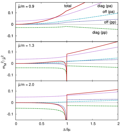
Figure 4: The dependence of $m_{M}^{2}$ (solid line) as well as the (pp) and (pa) contributions, defined in Eqs. (21) through (24), versus $\Delta/\delta\mu$ for three different values of $\bar{\mu}/m$ and a fixed value of $m/\Lambda=0.2$.

As one can see from the top panel of Fig. 4, the result for $m_{M}^{2}$ is positive definite in the case $\bar{\mu}/m=0.9$. This is not so, however, when the value of the ratio $\bar{\mu}/m$ is larger than 1. In particular, the quantity $m_{M}^{2}$ develops a negative divergence just below $\Delta/\delta\mu=1$ and stays negative for a range of values of $\Delta/\delta\mu$, see the middle and bottom panels in Fig. 4. It is easy to figure out that the divergence is caused by the singular behavior of the density of states around the effective Fermi surfaces in the gapless phases. This singularity affects only the particle-particle contributions, i.e., $(m_{M}^{2})_{\rm diag}^{(pp)}$ and $(m_{M}^{2})_{\rm off}^{(pp)}$. When the value of $\bar{\mu}/m$ becomes larger than 1 and increases further, negative values of $m_{M}^{2}$ first appear only near $\Delta/\delta\mu=1$ (see, e.g., the middle panel in Fig. 4). When the ratio $\bar{\mu}/m$ gets larger than about $1.8$, however, the quantity $m_{M}^{2}$ becomes negative in the whole range $\Delta/\delta\mu<1$ (see, e.g., the bottom panel in Fig. 4).

The numerical results for the screening mass can be conveniently summarized in Fig. 2 by identifying the region in which $m_{M}$ is imaginary (i.e., $m_{M}^{2}<0$). For the given set of parameters, $\delta\mu/m=0.5$ and $m/\Lambda=0.2$, this is marked by the shaded area there. For $\bar{\mu}/m\gtrsim 1.8$, the gSC(2) type gapless phase is unstable in the whole range $\Delta/\delta\mu<1$ where it is defined. This is in agreement, of course, with the results at weak coupling HS04 . It is most interesting, however, that for smaller values of the ratio $\bar{\mu}/m$, the quantity $m_{M}^{2}$ could be positive even in the gapless phases. In particular, $m_{M}^{2}>0$ in the whole gSC(1) region as well as in a part of the gSC(2) region. Note that the gapless phases found in the diagram in Fig. 3 always correspond to the stable region.

To complete the analysis of the stability of gapless phases at strong coupling, we note that a general requirement is that the eigenvalues of the susceptibility matrix, $-\partial^{2}V/\partial\mu_{i}\partial\mu_{j}$, are non-negative PWY05 . As a criterion for stability, the susceptibility matrix is meaningful only in the ground state defined by that $\Delta(\bar{\mu},\delta\mu)$ which solves the gap equation. In a sense, therefore, the susceptibility criterion has a less general status than the one of the (chromo-)magnetic stability. The latter does not refer to a specific form of the gap equation. This difference might be very important when additional constraints (e.g., neutrality) are enforced on the system.

In the MF approximation used in this study, the eigenvalues of the susceptibility matrix are non-negative in all phases of Fig. 3, as well as in the regions to the left of the dashed lines in Fig. 2. We argue that this is related directly to the fact that the ground state is defined as the global minimum of the effective potential. Indeed, one of the important necessary conditions for the susceptibility criterion to be satisfied reads PWY05

$$-\frac{\partial^{2}V}{\partial(\delta\mu)^{2}}\geq 0.$$ (25)

In the model at hand, as one can easily check, this is equivalent to

$$\frac{\partial^{2}V}{\partial\Delta^{2}}\geq 0,$$ (26)

which is always satisfied at the global minimum of the effective potential.

Before concluding this section, we would like to briefly discuss the properties at the splitting point S in Fig. 2. This point describes the situation when the two effective Fermi surfaces merge exactly at zero momentum. This coincides with the definition in Ref. SS05 where the properties near S are studied using an effective theory approach. From Fig. 2 we see that four qualitatively different regions merge at point S, i.e., (i) gSC(1), (ii) SC, (iii) gSC(2) with a positive value of $m_{M}^{2}$, and (iv) gSC(2) with a negative value of $m_{M}^{2}$. This topology is in agreement with the qualitative picture presented in Ref. SS05 , although here we use a different approach. It is interesting, though, that the ground state defined by the splitting point is never realized in the MF approximation in our model. This is because the second derivative of the thermodynamic potential is negative definite at the point S, which excludes the possibility of having a minimum there.

V Discussion and Summary

In this paper, we explored the superconducting (superfluid) phases in a relativistic model with two fermion species having mismatched Fermi surfaces. We found that, in general, there could exist gapless phases with either one or two effective Fermi surfaces. In the MF approximation, however, only the gapless phase gSC(1) is realized as a ground state, and only at strong coupling. We also calculated the fermion-number current-current correlator in the static and long wave-length limit. The results show that the gapless phases at strong coupling are free of the (chromo-)magnetic instability. This is in contrast to the situation in neutral quark matter at weak coupling HS04 .

It is interesting to note that there could exist different regimes of BEC in the model at hand. In general, bound bosonic states are formed when $\bar{\mu}/m<1$ NSR85 . As seen from Fig. 2, this is satisfied in parts of the SC and gSC(1) regions, giving rise to gapped and gapless phases, respectively. While the number densities of the two species of fermions are equal in the former, there is an excess of one of the species in the latter. In fact, this excess is an order parameter that defines the gapless phases at zero temperature SH03 . The gapless BEC phase is a mixture of tightly-bound bosons in the form of a condensate and additional unpaired fermions SS05 ; PWY05 .

It is worth mentioning that the gapless phase of the gSC(1) type could also exist for a range of parameters when $\bar{\mu}/m>1$. In this case, stable bosons do not exist and, thus, the BEC regime cannot be realized. If the diquark coupling in quark matter is sufficiently strong, this gapless phase can potentially be realized as the ground state of baryon matter. Our analysis of the one-loop fermion contribution to the current-current correlator suggests that the gSC(1) phase is stable. In the case of quark matter, however, it might be important to check if the inclusion of gluon and ghost contributions does not change the conclusion. While such contributions are negligible in the weak-coupling limit, this may not be the case at strong coupling.

A few words are in order regarding non-relativistic models SS05 ; PWY05 ; SheehyRadzihovsky ; KunYang ; SachdevYang . In our analysis, we saw that purely relativistic effects due to the antiparticle-antiparticle loops were always small near the splitting point. This suggests strongly that our results should remain qualitatively the same also in the non-relativistic limit that is defined by $|\bar{\mu}-m|/m\ll 1$, $\delta\mu/m\ll 1$ and $\Delta/m\ll 1$. Indeed, these conditions define a narrow area around the vertical line $\bar{\mu}/m=1$ in Fig. 2 which includes the point S. In fact, this also suggests that the topology around the splitting point is the same in both relativistic and non-relativistic models.

Note added. While finishing this paper, we learned that a similar study in a non-relativistic model is done by E. Gubankova, A. Schmitt, and F. Wilczek GSW06 .

References

- (1) C. A. Regal, M. Greiner, and D. S. Jin, Phys. Rev. Lett. 92, 040403 (2004); M. Bartenstein et. al., Phys. Rev. Lett. 92, 120401 (2004); M. W. Zwierlein et. al., Phys. Rev. Lett. 92, 120403 (2004); J. Kinast et. al., Phys. Rev. Lett. 92, 150402 (2004); T. Bourdel et. al., Phys. Rev. Lett. 93, 050401 (2004); M. W. Zwierlein et. al., cond-mat/0511197. G. B. Partridge et. al., cond-mat/0511752.
- (2) B. C. Barrois, Nucl. Phys. B 129, 390 (1977); D. Bailin and A. Love, Phys. Rep. 107, 325 (1984).
- (3) M. Alford, K. Rajagopal, and F. Wilczek, Phys. Lett. B 422, 247 (1998); R. Rapp, T. Schäfer, E. V. Shuryak, and M. Velkovsky, Phys. Rev. Lett. 81, 53 (1998).
- (4) K. Rajagopal and F. Wilczek, hep-ph/0011333; M. Alford, Ann. Rev. Nucl. Part. Sci. 51, 131 (2001); T. Schäfer, hep-ph/0304281; D. H. Rischke, Prog. Part. Nucl. Phys. 52, 197 (2004); H.-C. Ren, hep-ph/0404074; M. Huang, Int. J. Mod. Phys. E 14 (2005) 675; I. A. Shovkovy, Found. Phys. 35 (2005) 1309.
- (5) M. G. Alford, K. Rajagopal, and F. Wilczek, Nucl. Phys. B 537, 443 (1999).
- (6) M. Alford and K. Rajagopal, JHEP 0206, 031 (2002).
- (7) A. W. Steiner, S. Reddy, and M. Prakash, Phys. Rev. D 66, 094007 (2002); M. Huang, P.F. Zhuang, and W.Q. Chao, Phys. Rev. D 67, 065015 (2003); F. Neumann, M. Buballa, and M. Oertel, Nucl. Phys. A 714, 481 (2003); S. B. Rüster and D. H. Rischke, Phys. Rev. D 69, 045011 (2004).
- (8) I. A. Shovkovy and M. Huang, Phys. Lett. B 564, 205 (2003); M. Huang and I. A. Shovkovy, Nucl. Phys. A 729, 835 (2003).
- (9) M. Alford, C. Kouvaris, and K. Rajagopal, Phys. Rev. Lett. 92, 222001 (2004); Phys. Rev. D 71, 054009 (2005).
- (10) M. Huang and I. A. Shovkovy, Phys. Rev. D 70, 051501(R) (2004); Phys. Rev. D 70, 094030 (2004).
- (11) R. Casalbuoni, R. Gatto, M. Mannarelli, G. Nardulli, and M. Ruggieri, Phys. Lett. B605, 362 (2005); M. Alford and Q.H. Wang, J. Phys. G 31, 719 (2005).
- (12) K. Fukushima, Phys. Rev. D 72, 074002 (2005).
- (13) S.-T. Wu and S. Yip, Phys. Rev. A 67, 053603 (2003);
- (14) K. Rajagopal and A. Schmitt, hep-ph/0512043.
- (15) S. B. Rüster, I. A. Shovkovy, and D. H. Rischke, Nucl. Phys. A 743, 127 (2004); S. B. Rüster, V. Werth, M. Buballa, I. A. Shovkovy, and D. H. Rischke, Phys. Rev. D 72, 034004 (2005); hep-ph/0509073.
- (16) K. Fukushima, C. Kouvaris, and K. Rajagopal, Phys. Rev. D 71, 034002 (2005).
- (17) K. Iida, T. Matsuura, M. Tachibana and T. Hatsuda, Phys. Rev. D 71, 054003 (2005); Phys. Rev. Lett. 93, 132001 (2004).
- (18) D. Blaschke, S. Fredriksson, H. Grigorian, A. M. Öztaş, and F. Sandin, Phys. Rev. D 72, 065020 (2005).
- (19) H. Abuki and T. Kunihiro, hep-ph/0509172; H. Abuki, M. Kitazawa and T. Kunihiro, Phys. Lett. B 615, 102 (2005).
- (20) M. Matsuzaki, Phys. Rev. D 62, 017501 (2000); H. Abuki, T. Hatsuda, and K. Itakura, Phys. Rev. D 65, 074014 (2002).
- (21) M. Kitazawa, T. Koide, T. Kunihiro, and Y. Nemoto, Phys. Rev. D 70, 056003 (2004); Prog. Theor. Phys. 114, 205 (2005).
- (22) Y. Nishida and H. Abuki, hep-ph/0504083.
- (23) K. Nawa, E. Nakano, and H. Yabu, hep-ph/0509029.
- (24) M. Kitazawa, T. Koide, T. Kunihiro, and Y. Nemoto, Phys. Rev. D 65, 091504 (2002).
- (25) D. N. Voskresensky, Phys. Rev. C 69, 065209 (2004); nucl-th/0306077.
- (26) L. He, M. Jin, and P. Zhuang, hep-ph/0511300.
- (27) D. T. Son and M. A. Stephanov, cond-mat/0507586.
- (28) G. Sarma, J. Phys. Chem. Solids 24, 1029 (1963).
- (29) E. Gubankova, W.V. Liu, and F. Wilczek, Phys. Rev. Lett. 91, 032001 (2003); W.V. Liu, F. Wilczek, and P. Zoller, Phys. Rev. A 70, 033603 (2004); M.M. Forbes, E. Gubankova, W.V. Liu, and F. Wilczek, Phys. Rev. Lett. 94, 017001 (2005).
- (30) S. Reddy and G. Rupak, Phys. Rev. C 71, 025201 (2005).
- (31) I. Giannakis and H. C. Ren, Nucl. Phys. B 723, 255 (2005); Phys. Lett. B 611, 137 (2005).
- (32) P. Nozières and S. Schmitt-Rink, J. Low Temp. Phys. 59, 195 (1985).
- (33) C.-H. Pao, S-T. Wu, and S.-K. Yip, cond-mat/0506437.
- (34) D. E. Sheehy and L. Radzihovsky, cond-mat/0508430.
- (35) K. Yang, cond-mat/0508484.
- (36) S. Sachdev and K. Yang, cond-mat/0602032.
- (37) E. Gubankova, A. Schmitt, and F. Wilczek, in preparation.