Third order Coulomb correction to $t\bar{t}$ threshold cross section

Abstract

We report on our result of third order Coulomb correction to the cross section $\sigma(e^{+}e^{-}\rightarrow t\bar{t})$ near threshold. Analytic expression for the Coulomb energy and wave function at the origin are obtained. We discuss the significance of the Coulomb correction to the threshold cross section and heavy quarkonium phenomenology.

1 Threshold cross section

The $t\bar{t}$ threshold cross section has the following schematic form in the conventional perturbative expansion of $\alpha_{s}$,

$$\sigma(e^{+}e^{-}\rightarrow t\bar{t})\sim\sigma_{\rm Born}\large[1+\frac{\alpha_{s}}{v}+\left(\frac{\alpha_{s}}{v}\right)^{2}+\cdots\,\large]\,,$$ (1)

where $\sigma_{\rm Born}$ is a Born cross section, and $v=\sqrt{1-4m_{t}^{2}/s}$ is speed of produced $t,\bar{t}$. The combination of $(\alpha_{s}/v)^{n}$ appears to all order in the perturbation theory, known as Coulomb singularity. The perturbative expansion in $\alpha_{s}$ is not applicable to the threshold cross section because $v$ is of order $\alpha_{s}$ near the $t\bar{t}$ threshold $\sqrt{s}\sim 2m_{t}$, and the Coulomb singularity $(\alpha_{s}/v)^{n}$ dominates the cross section. To obtain meaningful cross section the Coulomb singularity has to be summed to all order in $\alpha_{s}$. The physical origin of the Coulomb singularity is instantaneous gluon exchange between $t$ and $\bar{t}$ which has a small spatial momentum $|\vec{q}|\sim v\sim 0$. This is called potential gluon because of its propagator

$$\widetilde{V}_{C}(\mbox{\boldmath${q}$})=-\frac{4\pi C_{F}\alpha_{s}}{\mbox{\boldmath${q}$}^{2}}\,,$$ (2)

where $C_{F}=4/3$, which is the Coulomb potential $V_{C}=-C_{F}\alpha_{s}/r$ in coordinate space.

This understanding leads to a quantum mechanical description which is equivalent to resummation of the Coulomb singularity. People had been looking for an effective field theory (EFT) which makes the resummation systematic. Finally a non-relativistic version of QCD was derived, called pNRQCD/vNRQCD [2, 3]. The EFT makes the resummation systematic based on nonrelativistic power counting $v\sim\alpha_{s}\ll 1$ in Lagrangian level. Nowadays we understand the resummation using the EFT, and higher order corrections are taken into account in the EFT framework systematically. The NNLO calculation for the total cross section was completed by several groups [4], and now we are working on the NNNLO corrections using the EFT.

The EFT classifies the corrections into three classes:

$\bullet$ Hard corrections included in Wilson coefficients of (composite) operators.
$\bullet$ Potential corrections, which are non-local (in space) 4-Fermi operators but local in time.
$\bullet$ Dynamical gluon corrections called ultra-soft gluon in the EFT.

The hard corrections are related to re-normalization of the operators in the EFT. The ultrasoft correction appears at NNNLO calculation, and the corresponding energy level correction is know by Kniehl-Penin [5]. However complete NNNLO correction to the total cross section is not known, yet. We discuss a part of the potential corrections in this report, which has the following form in the EFT Lagrangian,

$$\delta{\cal L}(x)=\int d^{3}{\mbox{\boldmath${r}$}}\big{[}\psi^{\dagger}\psi\big{]}(x+\mbox{\boldmath${r}$})V(\mbox{\boldmath${r}$})\big{[}\chi^{\dagger}\chi\big{]}(x)\,,$$ (3)

where $\psi^{\dagger},\chi$ is a creation operator of heavy quark and anti-quark, respectively. We will report on the result of the Coulomb correction.

We parameterize the momentum space Coulomb potential as follows

$$\widetilde{V}(\mbox{\boldmath${q}$})=\widetilde{V}_{C}(\mbox{\boldmath${q}$})\,\big{[}1+\widetilde{\cal V}_{1}(\mbox{\boldmath${q}$})+\widetilde{\cal V}_{2}(\mbox{\boldmath${q}$})+\widetilde{\cal V}_{3}(\mbox{\boldmath${q}$})\big{]},$$ (4)

where ${\cal V}_{n}(\mbox{\boldmath${q}$})$ is n-th order correction to the pure Coulomb potential $\widetilde{V}_{C}$, induced by loop diagrams when the EFT is derived from QCD. Explicit form of the potentials were derived at NNNLO (except $a_{3}$) in ref. [6], and the Coulomb potential reads

$$\widetilde{\cal V}_{1}=\frac{\alpha_{s}}{4\pi}\big{[}a_{1}+\beta_{0}\,l_{q}\,\big{]}$$

$$\widetilde{\cal V}_{2}=\left(\frac{\alpha_{s}}{4\pi}\right)^{\!2}\big{[}a_{2}+\big{(}2a_{1}\beta_{0}+\beta_{1}\big{)}\,l_{q}+\beta_{0}^{2}\,l_{q}^{2}\,\big{]}$$

$$\widetilde{\cal V}_{3}=\left(\frac{\alpha_{s}}{4\pi}\right)^{\!3}\big{[}a_{3}+8\pi^{2}C_{A}^{3}\,l_{q}(\nu)+\big{(}3a_{2}\beta_{0}+2a_{1}\beta_{1}$$

$$+\beta_{2}\big{)}\,l_{q}+\,\big{(}3a_{1}\beta_{0}^{2}+\frac{5}{2}\beta_{0}\beta_{1}\big{)}\,l_{q}^{2}+\beta_{0}^{3}\,l_{q}^{3}\,\big{]},$$ (5)

where $l_{q}=\ln(\mu^{2}/\mbox{\boldmath${q}$}^{2})$ and $l_{q}(\nu)=\ln(\nu^{2}/\mbox{\boldmath${q}$}^{2})$, $\beta_{i}$ are the coefficients of QCD $\beta$-function. The scale $\mu$ is QCD renormalization scale, and the $\nu$ in ${\cal V}_{3}$ is a scale introduced to separate the ultrasoft and potential modes in the EFT. Physical quantities are scale independent if all the corrections at given order are taken into account (see for instance [7]). Now our task is to calculate the threshold cross section using the EFT Lagrangian eq.(3) with the Coulomb potential eqs.(4), (5).

2 Green function method

We use the optical theorem to calculate the threshold total cross section which tells us that the cross section can be obtained by taking the imaginary part of the correlation function of production currents

$$\sigma(e^{+}e^{-}\rightarrow t\bar{t})=\frac{18\pi e_{t}^{2}}{m_{t}^{2}}{\rm Im}G(E+i\Gamma_{t}),$$

$$G=\frac{i}{N_{c}}\int d^{4}xe^{iqx}\langle{\rm vac}|[\psi^{\dagger}\chi](x)[\chi^{\dagger}\psi](0)|{\rm vac}\rangle,$$ (6)

where $N_{c}=3$ and $m_{t}$ is the quark pole mass. Using the EFT one can show that the matrix element $G(E)$ can be expressed by the quantum mechanical Green function

$$G(E)=\langle 0|\hat{G}(E)|0\rangle=\langle 0|\,\frac{1}{\frac{\mbox{\boldmath${p}$}\,^{2}}{m_{t}}+V(\mbox{\boldmath${r}$})-E}\,|0\rangle\,,$$ (7)

where $|0\rangle$ denotes a quantum mechanical position eigenstate at the origin $\mbox{\boldmath${r}$}=0$. At this stage we perform quantum mechanical perturbation theory by expanding the denominator of the Green function with respect to the higher order Coulomb potentials. The third order corrections read

$$\delta_{3}\hat{G}=-\,\hat{G}_{0}\delta V_{3}\hat{G}_{0}+\,2\hat{G}_{0}\delta V_{1}\hat{G}_{0}\delta V_{2}\hat{G}_{0}$$

$$-\,\hat{G}_{0}\delta V_{1}\hat{G}_{0}\delta V_{1}\hat{G}_{0}\delta V_{1}\hat{G}_{0}\,.$$ (8)

Here $G_{0}=(\mbox{\boldmath${p}$}^{2}/m_{t}-E)^{-1}$ is the zeroth order Green function, $\delta V_{n}\equiv[{\cal V}_{n}\,V_{C}](r)$ is the n-th order Coulomb potential. We calculated the expanded Green function semi-analytically and obtained double sum representations, which were evaluated numerically [1].

The Green function $G(E)$ has a single pole at the bound-state energy level $E=E_{n}$,

$$G(E)\stackrel{{\scriptstyle E\to E_{n}}}{{=}}\frac{|\psi_{n}(0)|^{2}}{E_{n}-E-i\epsilon}+\mbox{non-singular}\,,$$ (9)

where $|\psi_{n}(0)|^{2}$ and $E_{n}$ is the bound-state wave function squared at the origin and energy level, respectively, which has series expansion in $\alpha_{s}$

$$E_{n}=E_{n}^{(0)}\,\big{[}1+\sum_{i=1}^{3}\left(\frac{\alpha_{s}}{4\pi}\right)^{i}e_{i}\,\big{]}\,,$$

$$|\psi_{n}(0)|^{2}=|\psi_{n}^{(0)}(0)|^{2}\,\big{[}1+\sum_{n}^{3}\left(\frac{\alpha_{s}}{4\pi}\right)^{i}f_{i}\,\big{]}\,,$$ (10)

where $E_{n}^{(0)},|\psi_{n}(0)|^{2}$ is the zeroth order result for the energy and wave function. By performing matching between expanded Green function eq.(8) and the pole structure of exact Green function eq.(9), we obtained analytical result [1] for $e_{i}$ and $f_{i}$ for the S-wave bound state at NNNLO. The expression is too lengthy to show here. In the next section we discuss phenomenological significance of the NNNLO Coulomb corrections using the obtained result.

3 Numerical analysis and Conclusion

Our formalism up to now is not specific to the top quark, actually it is applicable to bottom quark system replacing $m_{t}$ and $n_{f}=5$ by $m_{b}$ and $n_{f}=4$ ($n_{f}$ exists in the $\alpha_{s}$ and $\beta$-function in the Coulomb potential.) We investigate the quarkonium energy levels and $t\bar{t}$ threshold cross section in the following.

In the phenomenological analysis we use the potential-subtracted (PS) mass [8] to make our prediction infrared renormalon free. The relation between the pole and PS masses is given by

$$m=m_{\rm PS}(\mu_{f})-\frac{1}{2}\int_{q\leq\mu_{f}}\frac{d^{3}{\mbox{\boldmath${q}$}}}{(2\pi)^{3}}\,\tilde{V}(\mbox{\boldmath${q}$})|_{\nu=\mu_{f}}\,,$$ (11)

where $\mu_{f}$ is infrared cutoff of order $m\alpha_{s}$. We take into account non-Coulomb corrections for quarkonium energy levels known from literatures [5, 6, 9, 10]. So the results are complete NNNLO as far as energy level is concerned.

3.1 Bottomonium masses

Using the analytical expression for the $e_{i},f_{i}$, we obtain the relation between mass of bottomonium and bottom quark. It might be instructive to show the results using pole and PS masses:

$$M_{\Upsilon(1S)}=2m_{b}+E_{1}^{(0)}\big{[}1+1.09_{\rm NLO}$$

$$+\big{(}1.42+0.36_{nC}\big{)}_{\rm N^{2}LO}+\big{(}2.29+0.28_{nC}\big{)}_{\rm N^{3}LO}\big{]}$$

$$=2m_{b,\rm PS}+E_{1,\rm PS}^{(0)}\big{[}1+0.19_{\rm NLO}$$

$$+\big{(}0.07-0.23_{nC}\big{)}_{\rm N^{2}LO}+\big{(}0.09-0.19_{nC}\big{)}_{\rm N^{3}LO}\big{]},$$

where $m_{b}=5$ GeV, $m_{\rm PS}(2GeV)=4.6$ GeV. The numbers are given separately for Coulomb and non-Coulomb to show numerical dominance of the former (in the pole scheme). One can see the presence of anomalously large Coulomb correction (IR renormalon) in the pole-mass scheme, while in the PS mass scheme this behavior is improved and convergence of the series became better.

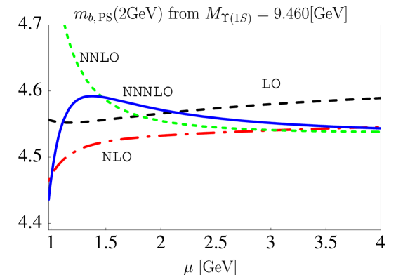
Figure 1: The bottom PS mass, $m_{b,\rm PS}(2\,\mbox{GeV})$ extracted from the Upsilon mass

We use the mass relation between $\Upsilon(1S)$ and $m_{b,{\rm PS}}$ to extract the bottom PS mass from the experimental value $M_{\Upsilon(1S)}|_{exp.}=9.460$ GeV. We obtained

$$m_{b,\rm PS}(2\,\mbox{GeV})=(4.57\pm 0.03_{\rm pert.}$$

$$\hskip 28.45274pt\pm 0.01_{\alpha_{s}}\pm 0.07_{\rm non-pert.})\,\,\mbox{GeV},$$ (12)

where the subscripts denote the source of errors.

In Fig.1 we show a scale dependence of the extracted PS mass $m_{b,{\rm PS}}(2{\rm GeV})$. Using extracted PS mass we are able to predict the masses of excited states of the spin triplet S-wave $\Upsilon$ family. In Fig.2 we show the $\Upsilon(2S)$ mass using $m_{b,PS}(2{\rm GeV})=4.57$ GeV as a function of the renormalization scale $\mu$. One can see that the large NNNLO corrections are preferable for scale $\mu>2$ GeV, however the prediction overshoots the experimental value $M_{\Upsilon(2S)}=10.023$ GeV at the lower scale. The naively expected natural scale for the bottomonium is $\mu=C_{F}\alpha_{s}m_{b,\rm PS}/n$ ($n$ is the principle quantum number), which is $\mu=1.23$ GeV for $\Upsilon(2S)$. This may indicate break down of perturbative computation for the excited $\Upsilon$ family. Similar behavior is observed for $\Upsilon(3S)$.

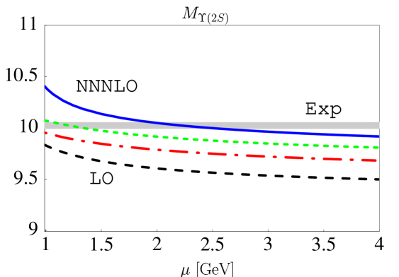
Figure 2: $\Upsilon(2S)$ mass as a function of scale $\mu$. The lines are plotted for LO(long dashes), NLO(long-short dashes), NNLO(dots), NNNLO(solid) and shaded band shows $M_{\Upsilon(2S)}|_{exp.}$.

3.2 Toponium

In future linear colliders remnant of toponium $1S$ resonance should be observed as a peak position of the $t\bar{t}$ cross section. This enables us to measure the $M_{t\bar{t}(1S)}$ and extract the top quark mass from the data. Here we perform an exercise, how precisely we can predict the 1S toponium mass when we fix the top quark mass as an input parameter. Adopting $m_{t,\rm PS}=175\,$GeV and $\mu=32.6\,$ GeV ($=C_{F}\alpha_{s}m_{t,\rm PS}$), we obtain

$$M_{t\bar{t}(1S)}=(350+0.85+0.05-0.13+0.01)\,\,{\rm GeV}$$

$$\hskip 17.07182pt=350.78\,\,\mbox{GeV}.$$ (13)

Scale variation between $15<\mu<60{\rm GeV}$ changes the total number only by $60$ MeV. The small higher order correction implies that precise top quark mass extraction is possible in principle, in the total cross section measurement. (There are several issues in the total cross section measurement at linear collider experiments, see for instance [11]). To obtain $\overline{\mathrm{MS}}$ mass, being more commonly used in high energy processes, from $M_{t\bar{t}(1S)}$ we need to know the relation between the PS and $\overline{\mathrm{MS}}$ masses at 4-loop order, which is currently unknown. Analysis using large-$\beta_{0}$ approximation to 4-loop $\overline{\mathrm{MS}}$ - pole mass relation and direct extraction of $\overline{\mathrm{MS}}$ mass from $M_{t\bar{t}(1S)}$ is available from ref.[12], which is consistent with our result.

3.3 The Coulomb wave function at the origin and Green function

In this subsection we discuss the Coulomb wave function and the Green function. Since the complete NNNLO non-Coulomb corrections and Wilson coefficient of the production current in EFT are unknown, we shall discuss only the Coulomb corrections. As we demonstrated in the previous section, applicability of this method to bottomonium system is doubtful due to large NNNLO correction and slow convergence. Thus we focus on the case of toponium Coulomb wave function and Green function.

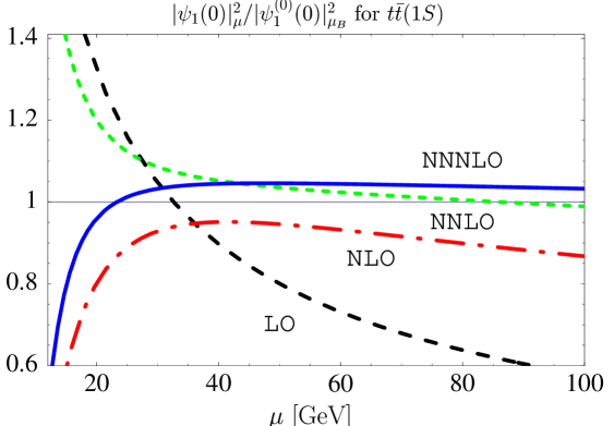
Figure 3: The Coulomb wave function at the origin squared as a function of the scale $\mu$.

We show numerical formula for the $1S$ toponium Coulomb wave function at the origin

$$\big{|}\psi_{1}(0)\big{|}^{2}_{C}=\frac{(m_{t}C_{F}\alpha_{s})^{3}}{8\pi}\big{[}1+\alpha_{s}\big{(}-0.4333$$

$$+3.661\,L\big{)}+\alpha_{s}^{2}\big{(}5.832-5.112\,L+8.933\,L^{2}\big{)}$$

$$+\,\alpha_{s}^{3}\big{(}-13.73+6.446\,\ln\big{(}\frac{\nu}{m_{t}C_{F}\alpha_{s}}\big{)}+39.72\,L$$

$$-22.91\,L^{2}+18.17\,L^{3}\big{)}\,\big{]}\,,$$ (14)

where $L=\ln(\mu/C_{F}\alpha_{s}m_{t})$. To draw Fig.3 we rewrote the eq.(14) using $m_{t,PS}(20{\rm GeV})=175$ GeV and took into account the mass correction eq.(11) at given order of nonrelativistic expansion consistently. The figure shows that perturbative corrections to the Coulomb wave function is reasonably small for $\mu>25$ GeV and the scale dependence is mild, while in lower scale $\mu<25$ GeV the corrections are too large so the perturbative expansion is unreliable in the lower region.

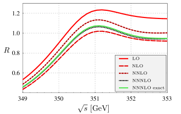
Figure 4: Top quark pair production (Coulomb corrections only) for $\mu=30$ GeV, successively including higher order corrections.

In Fig.4 we show the $t\bar{t}$ threshold cross section as a function of CM energy for $m_{t,\rm PS}(20{\rm GeV})=175$ GeV including only the Coulomb correction successively from LO to NNNLO. The line denoted as “NNNLO exact” is a cross section obtained by numerically solving shröding equation for the Green function using NNNLO Coulomb potential. The result show a convergence of the perturbative approximation to the NNNLO-exact line.

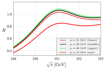
Figure 5: The NNNLO $t\bar{t}$ cross section ( Coulomb corrections only) for $\mu=15,30,60$ GeV for the perturbative approximation, and $\mu=15$ GeV for the NNNLO exact result.

In Fig.5 we show the scale dependence of NNNLO cross section for the perturbative Green function with $\mu=15,30,60$ GeV, and $\mu=15$ GeV for NNNLO-exact. The exact Green function is stable against scale variation (so we showed only the case $\mu=15$ GeV), while perturbative Green function (cross section) is unstable against scale variation from 15 to 30 GeV (moderate change from $\mu=30$ to 60 GeV). This is consistent with wave function analysis, where the higher order corrections were large for $\mu<25$ GeV, so we may conclude that the perturbative expansion is not reliable in lower scale region. The NNNLO-exact contains higher order insertions of the Coulomb potential to all order in eq.(8). The perturbative cross section agrees well with NNNLO-exact for large scale where it is supposed to be reliable from the wave function analysis. We believe that the NNNLO-exact cross section is reliable in wider range of $\mu$, and the perturbative cross section is reliable only in the region $\mu>25$ GeV. Indeed we find that the multiple insertions of the Coulomb potential give large contributions to the perturbative Green function, and is slowly converging at small scale. Thus we conclude that the “correct” scale choice for the perturbative (Coulomb) cross section is $\mu>25$, while choice of small scale may lead to misleadingly large uncertainties. We estimated yet unknown higher order Coulomb corrections should be less than 5 %.

Acknowledgements
Y.K. would like to thank M. Beneke and K. Schuller for useful discussion, and for reading this manuscript. Y.K. thanks J. Kodaira for invitation to the RADCOR05 conference.

References

- [1] M. Beneke, Y. Kiyo and K. Schuler, Nucl. Phys. B714 (2005) 67.
- [2] A. Pineda and J. Soto, Nucl. Phys. Proc. Suppl. 64 (1998) 428 [hep-ph/9707481].
- [3] M. E. Luke, A. V. Manohar and I. Z. Rothstein, Phys. Rev. D 61 (2000) 074025.
- [4] A. H. Hoang et al., Eur. Phys. J. direct C 2 (2000) 1, and references therein.
- [5] B. A. Kniehl and A. A. Penin, Nucl. Phys. B 563 (1999) 200.
- [6] B.A. Kniehl, A.A. Penin, V.A. Smirnov and M. Steinhauser, Nucl. Phys. B 635 (2002) 357.
- [7] N. Brambilla, A. Pineda, J. Soto and A. Vairo, Nucl. Phys. B 566 (2000) 275.
- [8] M. Beneke, Phys. Lett. B 434 (1998) 115.
- [9] A. A. Penin and M. Steinhauser, Phys. Lett. B 538 (2002) 335.
- [10] A. A. Penin, V. A. Smirnov and M. Steinhauser, Nucl. Phys. B 716 (2005) 303.
- [11] A. Juste et al., Report of the 2005 Snowmass Top/QCD Working Group [hep-ph/0601112].
- [12] Y. Kiyo and Y. Sumino, Phys. Rev. D 67 (2003) 071501