Finite Temperature Spectral Densities of Momentum and R-Charge Correlators in $\mathcal{N}=4$ Yang Mills Theory

Abstract

We compute spectral densities of momentum and R-charge correlators in thermal $\mathcal{N}=4$ Yang Mills at strong coupling using the AdS/CFT correspondence. For $\omega\sim T$ and smaller, the spectral density differs markedly from perturbation theory; there is no kinetic theory peak. For large $\omega$, the spectral density oscillates around the zero-temperature result with an exponentially decreasing amplitude. Contrast this with QCD where the spectral density of the current-current correlator approaches the zero temperature result like $(T/\omega)^{4}$. Despite these marked differences with perturbation theory, in Euclidean space-time the correlators differ by only $\sim 10\%$ from the free result. The implications for Lattice QCD measurements of transport are discussed.

I Introduction

The experimental relativistic heavy ion program has produced a variety of evidences which suggest that a Quark Gluon Plasma (QGP) has been formed at the Relativistic Heavy Ion Collider (RHIC) Bellwied:2005kq ; Adcox:2004mh . The relative success of hydrodynamic approaches Ollitrault:1992bk ; Hirano:2004er ; Teaney:2001av ; Kolb:2000fh ; Huovinen:2001cy suggests that the mean free path of the QGP is of order the thermal wave length $\sim T$ Molnar:2001ux . This bold inference requires further theoretical and experimental corroboration.

Theoretically, transport coefficients have been computed in the perturbative QGP using kinetic theory Baymetal ; AMY6 . However, it is important to obtain non-perturbative estimates for the transport properties of the medium. Kubo formulas relate hydrodynamic transport coefficients to the small frequency behavior of correlation functions of conserved currents in real time Forster ; BooneYip . In imaginary time correlation functions may be obtained from Lattice QCD measurements. Therefore, with a good model for the spectral density, one could hope to obtain a reasonable non-perturbative estimate for the transport properties of the QGP from Lattice QCD measurements. Recently, attempts to extract the shear viscosity nakamura97 ; nakamura05 and electric conductivity gupta03 have been made. More generally, the current-current correlator is being studied actively in order to extract interesting physical effects, e.g. dilepton emission, Landau damping, heavy quark diffusion, and in medium modifications of $J/\psi$. Peter_light ; Peter_heavy ; teaneyd ; Aarts:2005hg ; Mocsy:2005qw ; Nakahara:1999vy .

Whenever there is a large separation between the transport time scales and the temperature $T$, Euclidean correlators are remarkably insensitive to transport coefficients aarts02 ; teaneyd . This has been studied in perturbation theory aarts02 , where the transport time scale is $1/(g^{4}T)$, and in a theory with a heavy quark, where the diffusion time scale is $M/T^{2}$ or longer teaneyd . This insensitivity to transport is because the dominant transport contribution to the Euclidean correlator is an integral over the spectral density which is governed by a sum rule – the $f$-sum rule. Whenever, there is a quasi-particle description, the leading transport contribution to the Euclidean current-current correlator is proportional to the static susceptibility times an average thermal velocity squared of the quasi-particle. Only with very accurate measurements and a solid understanding of the spectral density can more transport information be gleaned from lattice correlators.

When there is no separation between the inverse temperature and transport time scales this conclusion requires further study. $\mathcal{N}=4$ Super Yang Mills (SYM) theory with a large number of colors and large ’t Hooft coupling provides a theory where there is no scale separation and where the spectral density can be computed if the Maldacena conjecture is accepted Maldacena:1997re . This conjecture states that $\mathcal{N}=4$ SYM is dual to classical type IIB supergravity on an $AdS\times S_{5}$ background Maldacena:1997re ; Gubser:1998bc ; Witten:1998qj . (See Ref. Aharony:1999ti for a review.) By solving the classical supergravity equations motion we may deduce the retarded correlators of strongly coupled $\mathcal{N}=4$ SYM.

Using the correspondence, Son, Policastro, and Starinets deduced the shear viscosity of strongly coupled $\mathcal{N}=4$ SYM Policastro:2001yc . Indeed the momentum diffusion constant is remarkably small, $\eta/(e+p)=1/4\pi T$. This result and subsequent calculations have led to the conjecture that the shear viscosity to entropy ratio is bounded from below, $\eta/s\geq 1/4\pi$ Kovtun:2004de ; Buchel:2004qq ; Policastro:2001yc . The correspondence was also used to calculate the R-charge diffusion coefficient, $D=1/(2\pi T)$ Policastro:2002se . This transport coefficient is also remarkably small although there is no conjectured bound associated with this medium property. It is interesting to compute the full spectral densities of these correlators following the framework set up in these works. With the spectral density in hand, the feasibility of extracting transport from the Lattice in a strong coupling regime can be assessed.

II Stress Tensor and R-charge Correlations

II.1 Stress Tensor Correlations

First let us recall the definitions Forster . The retarded correlators of $T^{00}$ and $T^{0i}$ are defined as follows

$$\chi_{ee}({\bf k},\omega) \equiv \int_{-\infty}^{\infty}dt\,\int d^{3}{\bf x}\,e^{+i\omega t-i{\bf k}\cdot{\bf x}}\,i\theta(t)\left\langle\left[T^{00}({\bf x},t),T^{00}(0,0)\right]\right\rangle\,,$$ (1)

$$\chi_{gg}^{ij}({\bf k},\omega) \equiv \int_{-\infty}^{\infty}dt\int d^{3}{\bf x}\,e^{+i\omega t-i{\bf k}\cdot{\bf x}}\,i\theta(t)\left\langle\left[T^{0i}({\bf x},t),T^{0j}(0,0)\right]\right\rangle\,.$$ (2)

$\chi_{gg}^{ij}$ is then decomposed into longitudinal and transverse pieces

$$\chi_{gg}^{ij}({\bf k},\omega)=\frac{k^{i}k^{j}}{k^{2}}\,\chi_{gg}^{L}({\bf k},\omega)+\left(\delta^{ij}-\frac{k^{i}k^{j}}{k^{2}}\right)\,\chi_{gg}^{T}({\bf k},\omega)\,.$$ (3)

Through linear response, hydrodynamics makes a definite prediction for these correlators at small $k$ and $\omega$ (see Appendix C for a review)

$$\chi_{gg}^{L}({\bf k},\omega) = (e+p)\,\frac{i\omega\Gamma_{s}k^{2}-(c_{s}k)^{2}}{\omega^{2}-(c_{s}k)^{2}+i\omega\Gamma_{s}k^{2}}\,,$$ (4)

$$\chi_{gg}^{T}({\bf k},\omega) = \frac{\eta k^{2}}{-i\omega+\frac{\eta k^{2}}{e+p}}\,,$$ (5)

where $e$ is the energy density, $p$ is the pressure, $\eta$ is the shear viscosity, $\zeta$ is the bulk viscosity, and $\Gamma_{s}=\frac{\frac{4}{3}\eta+\zeta}{e+p}$ is the sound attenuation length. Using energy conservation we deduce

$$\chi_{ee}({\bf k},\omega)=\frac{\omega^{2}}{k^{2}}\chi_{gg}^{L}\,.$$ (6)

Similarly we define the correlators of momentum fluxes

$$\chi_{\tau\tau}^{iljm}({\bf k},\omega)=\int_{-\infty}^{\infty}dt\,\int d^{3}{\bf x}\,e^{+i\omega t-i{\bf k}\cdot{\bf x}}\,i\theta(t)\left\langle[T^{il}({\bf x},t),T^{jm}(0,0)]\right\rangle\,.$$ (7)

Then using momentum conservation, we deduce that

$$\chi^{xxxx}_{\tau\tau} \equiv \frac{k^{i}k^{l}k^{j}k^{m}}{k^{4}}\chi_{\tau\tau}^{il,jm}({\bf k},\omega)=\frac{\omega^{2}}{k^{2}}\,\chi_{gg}^{L}({\bf k},\omega)\,,$$ (8)

$$\chi^{yxyx}_{\tau\tau} \equiv \frac{1}{2}\left(\delta^{ij}-\frac{k^{i}k^{j}}{k^{2}}\right)\,\frac{k^{l}k^{m}}{k^{2}}\,\chi_{\tau\tau}^{il,jm}({\bf k},\omega)=\frac{\omega^{2}}{k^{2}}\,\chi_{gg}^{T}({\bf k},\omega)\,.$$ (9)

The notation follows by assuming that ${\bf k}$ points in the $x$ direction.

We will concentrate on the transverse piece of the momentum correlator. We define the spectral density as follows

$$\rho_{\tau\tau}^{yxyx}({\bf k},\omega)=\frac{\mbox{Im}\chi_{\tau\tau}^{yxyx}({\bf k},\omega)}{\pi}\,.$$ (10)

Using the functional form in Eq. (5) we deduce the Kubo formula

$$\lim_{\omega\rightarrow 0}\lim_{k\rightarrow 0}\frac{\pi\rho_{\tau\tau}^{yx,yx}({\bf k},\omega)}{\omega}=\eta\,.$$ (11)

Euclidean correlators $G^{yxyx}_{\tau\tau}({\bf x},\tau)=\left\langle T^{yx}_{E}({\bf x},\tau)T^{yx}_{E}(0)\right\rangle$ can be deduced from the spectral density

$$G_{\tau\tau}^{yxyx}({\bf k},\tau)=\int_{0}^{\infty}d\omega\,\rho_{\tau\tau}^{yxyx}({\bf k},\omega)\frac{\cosh\left(\omega\left(\tau-\beta/2\right)\right)}{\sinh\left(\omega\beta/2\right)}\,.$$ (12)

Further explanation of the Euclidean definitions and conventions adopted in this work may be found in teaneyd .

The retarded correlator $\chi_{\tau\tau}^{yxyx}({\bf k},\omega)$ may computed using the AdS/CFT correspondence. The stress tensor couples to metric fluctuations $h_{xy}$ in the background of the black hole. We start with equation Eq. (6.6) of Policastro, Son and Starinets Policastro:2002se for the fluctuation $\phi\equiv h^{x}_{y}$ in the gravitational background. The linearized equations of motion for this field in the background are

$$\phi^{\prime\prime}_{k}-\frac{1+u^{2}}{uf}\phi^{\prime}_{k}+\frac{\mathfrak{w}^{2}-\mathfrak{q}^{2}(1-u^{2})}{uf^{2}}\phi_{k}=0\,.$$ (13)

Here $\phi_{k}$ is the Fourier transform of $\phi$ with respect to four momentum $k=(\omega,0,0,q)$ and we have defined $\mathfrak{w}\equiv\omega/(2\pi T)$, $\mathfrak{q}\equiv q/(2\pi T)$, and $f\equiv(1-u^{2})$. $u=1$ corresponds to the the event horizon of the black hole; $u=0$ corresponds to spatial infinity. We will integrate this equation and set $\mathfrak{q}=0$ in what follows.

Let us indicate the general strategy. Near the horizon $u=1$, we develop the series solutions Morse

$$\phi_{1} = (1-u)^{-i\mathfrak{w}/2}\left[1+(1-u)\left(\,\frac{\frac{3\mathfrak{w}^{2}}{4}-i\frac{\mathfrak{w}}{4}+i\frac{\mathfrak{w}^{3}}{2}}{1+\mathfrak{w}^{2}}\right)+\dots\right]\,,$$ (14)

$$\phi_{2} = \overline{\phi_{1}}\,,$$ (15)

where ${\overline{\phi_{1}}}$ denotes the complex conjugate of $\phi_{1}$. The physical solution is $\phi_{1}$ and not $\overline{\phi_{1}}$. Similarly near spatial infinity $u=0$, we can develop a power series solution of this equation. These solutions are

$${\Phi}_{1} = u^{2}\left[1-\frac{\mathfrak{w}^{2}}{3}u+\dots\right]\,,$$ (16)

$${\Phi}_{2} = -\frac{\mathfrak{w}^{4}}{2}\,\log(u){\Phi}_{1}+\left[1+\mathfrak{w}^{2}u+\left(\frac{1}{2}-\frac{29}{72}\mathfrak{w}^{4}\right)u^{2}+\dots\right]\,.$$ (17)

We note that ${\Phi}_{1}$ and ${\Phi}_{2}$ are real functions. Generally ${\Phi}_{i}$ will be a linear combination $\phi_{1}$ and $\overline{\phi_{1}}$. Following Policastro:2002se , the physically correct solution of Eq. (13) is $\phi_{1}$ which is a linear combination ${\Phi}_{1}$ and ${\Phi}_{2}$:

$$\phi_{1}=A{\Phi}_{2}+B{\Phi}_{1}\,.$$ (18)

We may set $A=1$ which is equivalent to the often assumed normalization condition $\left.\phi_{1}(u)\right|_{u=0}=1$ . Then the retarded Greens function is related by the correspondence to $\phi_{1}$

$$\chi_{\tau\tau}^{yxyx}({\bf q},\omega)=\frac{\pi^{2}N^{2}T^{4}}{4}\;\lim_{u\rightarrow 0}\frac{f}{u}(\phi_{-k})_{1}\partial_{u}(\phi_{k})_{1}\,,$$ (19)

where $(\phi_{k})_{1}$ denotes the $\phi_{1}$ which solves Eq. (13) with $k=(\omega,{\bf q})$. Using the power series expansion near $u\approx 0$, and the fact that ${\Phi}_{1}$ and ${\Phi}_{2}$ are real, we have the spectral density

$$\frac{\pi\rho_{\tau\tau}^{yxyx}(\omega)}{\omega}\equiv\frac{{\rm Im}\chi_{\tau\tau}^{yxyx}(\omega,{\bf q})}{\omega} = \frac{\pi^{2}N^{2}T^{4}}{4}\,{\rm Im}B\,\lim_{u\rightarrow 0}\frac{f}{u}{\Phi}_{2}\partial_{u}({\Phi}_{1})\,,$$ (20)

$$= \frac{\pi^{2}N^{2}T^{4}}{4}\,2\,{\rm Im}B\,.$$ (21)

Thus the algorithm may divided into four steps: (1) Start at small $u\approx 0$ and use the power series to find the initial condition and first derivative of ${\Phi}_{1}$ and ${\Phi}_{2}$. (2) Integrate ${\Phi}_{1}$ and ${\Phi}_{2}$ forward to determine the solution close to $u\approx 1$. (3) Using the power series close to $u\approx 1$ determine the linear combination of $\phi_{1}$ and $\overline{\phi_{1}}$ that is ${\Phi}_{1}$. Also do this for ${\Phi}_{2}$. (4) Then determine the linear combination of ${\Phi}_{1}$ and ${\Phi}_{2}$ that is $\phi_{1}$. This fixes $B$ in Eqs. (18) and (21), and consequently determines the spectral density at the frequency specified in Eq. (13).

This algorithm was followed and the resulting spectral density is shown in Fig. 1(a). When the frequency $\mathfrak{w}$ is large we may follow this algorithm analytically and obtain the zero temperature result at large frequency. This is done in Appendix B and the resulting solution provides a good check of the numerical work. Further discussion of this figure in provided in Section III.

II.2 R-Charge Diffusion

A similar program may be followed to calculate the spectral density of the current-current correlator. First let us recall the definitions. Through linear response Forster ; teaneyd , the diffusion equation predicts that the density-density correlator

$$\chi_{\scriptscriptstyle NN}({\bf k},\omega)=\int_{-\infty}^{\infty}dt\,\int d^{3}{\bf x}\,e^{+i\omega t-i{\bf k}\cdot{\bf x}}\,i\theta(t)\left\langle\left[J^{0}_{a}({\bf x},t),J^{0}_{a}(0,0)\right]\right\rangle\qquad\mbox{(no $a$ sum)}\,,$$ (22)

has the following form at small $k$ and $\omega$

$$\chi_{\scriptscriptstyle NN}(k,\omega)=\frac{\chi_{s}Dk^{2}}{-i\omega+D\,k^{2}}\,,$$ (23)

where $\chi_{s}$ is the static R-charge susceptibility. The spatial current-current correlator is defined similarly

$$\chi_{\scriptscriptstyle JJ}^{ij}({\bf k},\omega)=\int_{-\infty}^{\infty}dt\,\int e^{+i\omega t-i{\bf k}\cdot{\bf x}}\,i\theta(t)\,\left\langle\left[J^{i}_{a}({\bf x},t),J^{j}_{a}(0,0)\right]\right\rangle\qquad\mbox{(no $a$ sum)}\,,$$ (24)

and may be broken up into longitudinal and transverse components

$$\chi_{\scriptscriptstyle JJ}^{ij}({\bf k},\omega)=\left(\frac{k^{i}k^{j}}{k^{2}}-\delta^{ij}\right)\,\chi_{\scriptscriptstyle JJ}^{T}({\bf k},\omega)+\frac{k^{i}\,k^{j}}{k^{2}}\,\chi_{\scriptscriptstyle JJ}^{L}({\bf k},\omega)\,.$$ (25)

The density-density correlator can be related to the longitudinal current-current correlator

$$\frac{\omega^{2}}{k^{2}}\chi_{\scriptscriptstyle NN}({\bf k},\omega)=\frac{k^{i}k^{j}}{k^{2}}\chi_{\scriptscriptstyle JJ}^{ij}({\bf k},\omega)=\chi_{\scriptscriptstyle JJ}^{L}({\bf k},\omega)\,.$$ (26)

For ${\bf k}=0$ there is no distinction between the longitudinal and transverse parts and therefore for $k\ll T$, $\chi_{\scriptscriptstyle JJ}^{L}({\bf k},\omega)\simeq\chi_{\scriptscriptstyle JJ}^{T}({\bf k},\omega)$.

The computation of these correlators at small ${\bf k}$ and $\omega$ has already been performed by Policastro, Son, and Starinets Policastro:2002se . From their computation (see Eq. 5.17b of that work) and the functional form of Eq. (23), the diffusion coefficient and static susceptibility are

$$D=\frac{1}{2\pi T}\,,\qquad\mbox{and}\qquad\chi_{s}=\frac{N^{2}T^{2}}{8}\,.$$ (27)

To extend this computation to finite frequency it is simplest to compute $\chi_{\scriptscriptstyle JJ}^{T}(0,\omega)$ which is uncoupled from the other modes. Since ${\bf k}=0$, $\chi_{JJ}^{T}(0,\omega)$ is equal to $\chi_{\scriptscriptstyle JJ}^{L}(0,\omega)$. Perturbations in the R-charge current couple to the Maxwell field and the equations of motion for the Maxwell field in the gravitational background have been worked out. Consider the Maxwell field $\phi$ transverse to ${\bf q}$, i.e. if ${\bf q}$ points in the $z$ direction then $\phi=A_{x}$. The equation of motion for the Fourier components of $\phi$ in the gravitational background reads

$$\phi_{k}^{\prime\prime}+\frac{f^{\prime}}{f}\,\phi_{k}^{\prime}+\frac{1}{uf}\left(\frac{\mathfrak{w}^{2}}{f}-\mathfrak{q}^{2}\right)\phi_{k}=0\;.$$ (28)

with $f=1-u^{2}$ and as before $k=(\omega,0,0,q)$, $\mathfrak{w}=\omega/(2\pi T)$ and $\mathfrak{q}=q/(2\pi T)$. In what follows we set $\mathfrak{q}=0$.

The procedure mirrors the stress tensor computation. Near $u=1$ we determine a power series solution

$$\phi_{1} = (1-u)^{-i\frac{\mathfrak{w}}{2}}\left[1+\dots\right]\,,$$ (29)

$$\phi_{2} = \overline{\phi_{1}}\,.$$ (30)

$\phi_{1}$ is the physical solution and not $\overline{\phi_{1}}$. Near $u=0$ we determine the power series

$${\Phi}_{1} = \mathfrak{w}u+\dots\,,$$ (31)

$${\Phi}_{2} = 1+\dots\;.$$ (32)

Integrating from $u\approx 0$ to $u\approx 1$ we determine the linear combination of ${\Phi}_{1}$ and ${\Phi}_{2}$ that is $\phi_{1}$

$$\phi_{1}={\Phi}_{2}+B\,{\Phi}_{1}\,.$$ (33)

Then the correspondence states that

$$\chi_{\scriptscriptstyle JJ}^{T}(0,\omega)=\frac{N^{2}T^{2}}{8}\lim_{u\rightarrow 0}f(\phi_{-k})_{1}\partial_{u}(\phi_{k})_{1}\;.$$ (34)

Since ${\Phi}_{2}$ and ${\Phi}_{1}$ are real and since ${\Phi}_{2}$ starts with one, the spectral density is

$$\frac{\pi\rho_{\scriptscriptstyle JJ}^{T,L}(0,\omega)}{\omega}\equiv\frac{\mbox{Im}\chi_{JJ}^{T}(0,\omega)}{\omega}=\frac{N^{2}T}{16\pi}\,\mbox{Im}\,B\,.$$ (35)

III Results

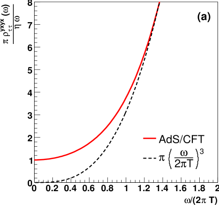
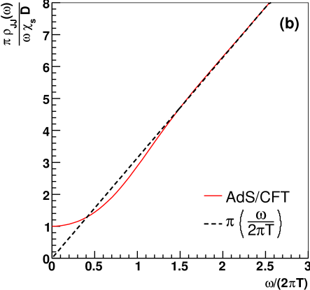
Figure 1: (a) The spectral density of the stress energy tensor, $\pi\rho_{\tau\tau}^{yxyx}(\omega)/\omega$ normalized by the shear viscosity, $\eta_{\scriptscriptstyle AdS}=\pi N^{2}T^{3}/8$. (b) The spectral density of the current-current correlator, $\pi\rho_{JJ}/\omega$ normalized by $\chi_{s}D=N^{2}T^{2}/16\pi T$. In both cases the dashed curves show the zero temperature results (Eq. (72) and Eq. (73)) normalized by the same factors. Due to a non-renormalization theorem in these channels, the zero temperature spectral densities in the free and interacting theories are equal Freedman:1998tz ; Chalmers:1998xr . At finite temperature the kinetic theory peak does not exist in the strongly interacting theory.

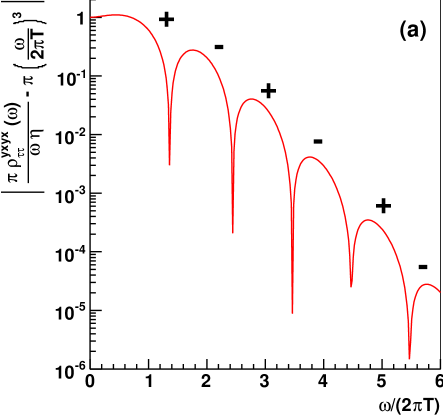
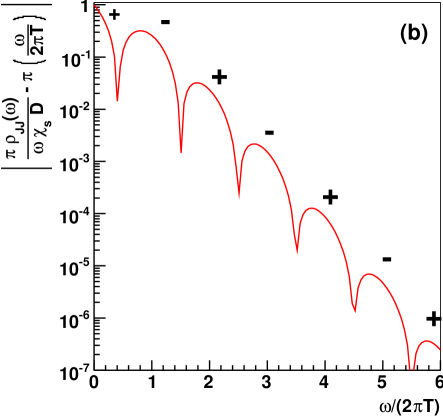
Figure 2: The spectral density of the (a) stress energy tensor and (b) current-current correlators as in Fig. 1 but the zero temperature result has been subtracted and the absolute value taken. The plus or minus indicates the sign. The finite temperature spectral densities oscillate around the zero temperature result with exponentially decreasing amplitude.

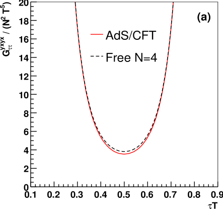
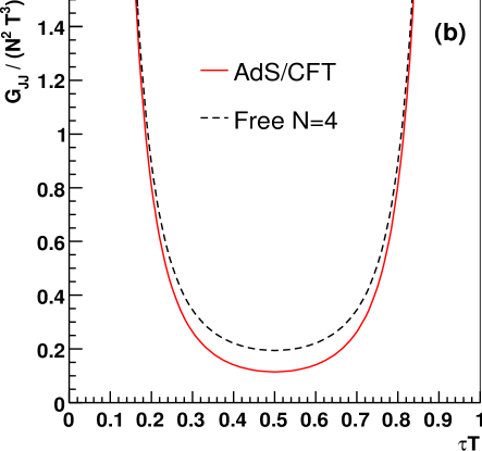
Figure 3: The Euclidean correlator for the (a) stress energy tensor correlator, $G^{yxyx}_{\tau\tau}$, and the (b) current-current correlator, $G_{JJ}$. The dashed curves show the free result for these Euclidean correlators.

The spectral density of the stress energy tensor

$$\rho^{yxyx}_{\tau\tau}(\omega)=\frac{1}{2\pi}\int_{-\infty}^{\infty}dt\,e^{+i\omega t}\int d^{3}{\bf x}\,\left\langle\left[T^{yx}({\bf x},t),T^{yx}({\bf 0},0)\right]\right\rangle\,,$$ (36)

is shown in Fig. 1(a). Similarly the spectral density for the R-charge current-current correlator

$$\rho_{{\scriptscriptstyle JJ}}(\omega)=\frac{1}{2\pi}\int_{-\infty}^{\infty}dt\,e^{+i\omega t}\int d^{3}{\bf x}\,\left\langle\left[J^{x}_{a}({\bf x},t),J^{x}_{a}({\bf 0},0)\right]\right\rangle\qquad\mbox{(no $a$ sum)}\,,$$ (37)

is shown in Fig. 1(b). These are normalized so that

$$\left.\frac{\pi\rho_{\tau\tau}^{yxyx}(\omega)}{\omega}\right|_{\omega=0}=\eta\,,\qquad\mbox{and}\qquad\left.\frac{\pi\rho_{{\scriptscriptstyle JJ}}(\omega)}{\omega}\right|_{\omega=0}=\chi_{s}D,$$ (38)

where $\eta$ is the shear viscosity, $\chi_{s}$ is the static R-charge susceptibility, and $D$ is the R-charge diffusion coefficient.

The remarkable feature of these spectral functions is the absence of any distinction between the transport time scales and the continuum time scales. For comparison, consider the spectral density of the stress energy tensor in the free theory as worked out in Appendix A. The full spectral density is a sum of the gauge, fermion, and scalar contributions

$$\left(\rho_{\tau\tau}^{yxyx}\right)_{\rm gauge} = \left(\frac{e+p}{5}\right)_{\scriptscriptstyle A}\omega\delta(\omega)+\frac{N^{2}}{160\pi^{2}}\,\left(1+2\,n_{B}\left(\omega\beta/2\right)\right)\,\omega^{4}\,,$$ (39)

$$\left(\rho_{\tau\tau}^{yxyx}\right)_{\rm fermion} = \left(\frac{e+p}{5}\right)_{\scriptscriptstyle\lambda}\omega\delta(\omega)+\frac{N^{2}}{160\pi^{2}}\,\left(1-2\,n_{F}\left(\omega\beta/2\right)\right)\,\omega^{4}\,,$$ (40)

$$\left(\rho_{\tau\tau}^{yxyx}\right)_{\rm scalar} = \left(\frac{e+p}{5}\right)_{\scriptscriptstyle X}\omega\delta(\omega)+\frac{N^{2}}{320\pi^{2}}\,\left(1+2\,n_{B}\left(\omega\beta/2\right)\right)\,\omega^{4}\,,$$ (41)

where for example $(e+p)_{\scriptscriptstyle X}$ is the partial enthalpy due to the free scalar fields – see Appendix A. The free spectral function for the current-current correlator has a similar structure and is recorded in the appendix. Notice the delta function at the origin. According to the $f$ sum rule (see below), perturbations will smear the delta-function at the origin but will not change the integral under the peak. The peak indicates a large separation between the transport and temperature scales and is what makes kinetic theory possible. It is hopeless to apply a quasi-particle description to the strongly coupled $\mathcal{N}=4$ case.

Also shown in Fig. 1(a) and (b) is the spectral density at zero temperature for the stress tensor and R-charge correlators. At zero temperature, the strongly coupled spectral densities are identical to the free $\mathcal{N}=4$ spectral densities as required by a non-renormalization theorem Freedman:1998tz ; Chalmers:1998xr . Fig. 2(a) and (b) show the absolute value of the difference between the finite temperature and zero temperature results on a log plot. The figure shows that the finite temperature result oscillates around the zero temperature result with exponentially decreasing amplitude. This is quite unusual and the exponential decrease is not due to any obvious Boltzmann factor. In QCD for instance, the spectral density of the current-current correlator approaches the zero temperature correlator as,  $\left(T/\omega\right)^{4}$   Altherr:1989jc ; Baier:1988xv . The author has no explanation for the strong coupling results in $\mathcal{N}=4$ SYM.

Finally, we may determine the corresponding Euclidean correlators by integrating the spectral density. For instance $G^{yxyx}_{\tau\tau}$ is determined from $\rho^{yxyx}_{\tau\tau}(\omega)$

$$G^{yxyx}_{\tau\tau}(\tau) = \int d^{3}{\bf x}\left\langle T^{yx}_{E}({\bf x},\tau)T^{yx}_{E}({\bf 0},0)\right\rangle\,,$$ (42)

$$= \int_{0}^{\infty}d\omega\,\rho_{\tau\tau}^{yxyx}(\omega)\frac{\cosh\left(\omega\left(\tau-\beta/2\right)\right)}{\sinh\left(\omega\beta/2\right)}\,.$$ (43)

The resulting Euclidean correlators for the stress tensor and current-current correlators are shown in Fig. 3(a) and (b) respectively. In each figure the strongly coupled case is compared to the free theory worked out in Appendix A.

First consider the stress tensor correlations. Although the spectral density in the strongly coupled theory is markedly different from the free theory, in Euclidean space-time the correlators differ only by 10%. This 10% difference is significantly smaller than the errors associated with this correlator on the lattice nakamura97 ; nakamura05 . At least from the perspective of the AdS/CFT correspondence, it is hopeless to measure the transport properties of the medium in the $T^{\mu\nu}$ channel where noisy gluonic operators dominate the signal. The figure also suggests that armed only with Euclidean measurements it is difficult to tell whether the theory is strongly interacting, i.e. whether there is a transport peak in the spectral density. Therefore, at least within the narrow framework of this work, rough agreement between quasi-particle calculations and lattice results Blaizot:2000fc ; Andersen:1999fw says little about the validity of the quasi-particle picture. Only precise agreement can firmly establish validity.

In weak coupling, the insensitivity to the transport time scale in the Euclidean correlator is readily understood from Eq. (43) and the free correlator Eqs. (39)–(41) teaneyd ; aarts02 . As perturbative interactions are turned on, the delta function at $\omega\sim 0$ is smeared by the inverse transport time scale. However, the integral under the peak remains the enthalpy times an average quasi-particle velocity squared, $\left\langle v_{\bf p}^{2}/5\right\rangle$. This is the physics content of the $f$-sum rule and is derived in Appendix D. When the smeared delta function is substituted into Eq. (43), the Euclidean correlator is roughly independent of the width of the peak, i.e. independent of the transport time scale. It seems that the strong coupling correlators remember this insensitivity to transport at weak coupling.

For the current-current correlator the difference between the free and interacting cases is slightly larger, $\sim 20\%$. Lattice measurements in the electromagnetic current-current channel are remarkably precise, $\sim 0.5$ – $2.0\%$ Peter_light ; Peter_heavy ; Nakahara:1999vy . This precision stems from the fact that the current-current channel correlates quark fields while the noisy $T^{\mu\nu}$ channel correlates gluonic fields. With hard work and precise data, the AdS/CFT correspondence would suggest that some information about transport can be extracted from Euclidean measurements in this channel. However even in the current-current case, one needs a definite strategy to isolate the low frequency contributions.

Note added. When this work was near completion, I learned that P. Kovtun and A. Starinets had nearly completed a similar computation Kovtun .

Acknowledgments. I thank Peter Arnold, Raju Venugopalan, Andrei Starinets, and Peter Petreczky for useful discussions. D. Teaney was supported by grants from the U.S. Department of Energy, DE-FG02-88ER40388 and DE-FG03-97ER4014.

Appendix A The Free Theory

The free $\mathcal{N}=4$ Lagrangian is written as follows:

$$\mathcal{L}=2\operatorname{tr}\left\{-\frac{1}{4}F^{2}+\frac{1}{2}\bar{\lambda}_{a}(-i\bar{\sigma}\cdot\partial)\lambda^{a}-\frac{1}{2}\partial_{\mu}X_{i}\partial^{\mu}X_{i}\right\}\,,$$ (44)

where “a” is a SU(4) index and “i” is a SO(6) index. Under flavor rotation, $\lambda^{a}$ transforms in the fundamental representation of SU(4) and $X^{i}$ transforms as the fundamental representation of SO(6). SU(4) and SO(6) are locally isomorphic. SU(4) matrices are parametrized as $e^{i\beta_{A}(T^{4})_{A}}$ with trace normalization $\operatorname{tr}[(T^{4})_{A}(T^{4})_{B}]=C_{4}\delta_{AB}$ and $C_{4}=1/2$. Similarly, SO(6) matrices are written as $e^{i\beta_{A}(T^{6})_{A}}$, with trace normalization $C_{6}=1$ Peskin . The normalization convention adopted here has been fixed so that the AdS/CFT correspondence holds at the level of two point functions at zero temperature Freedman:1998tz ; Chalmers:1998xr .

Using the Noether method we compute the conserved R-charge current

$$J^{\mu}_{A}=2\,\operatorname{tr}\left\{\left(\frac{T_{A}}{2}\right)_{ij}X_{i}{-i\overleftrightarrow{\partial^{\mu}}}X_{j}+(T_{A})_{ab}\bar{\lambda}_{a}\left(\frac{\bar{\sigma}^{\mu}}{2}\right)\lambda_{b}\right\}\,,$$ (45)

where $\overleftrightarrow{\partial}\equiv\overrightarrow{\partial}-\overleftarrow{\partial}$ and gives symmetric Feynman rules. The spectral density $\rho_{JJ}^{L}(\omega)$ is easily computed at ${\bf k}=0$; the details of a similar computation appear explicitly in an appendix of Ref. teaneyd . The full spectral density is

$$\rho_{{\scriptscriptstyle JJ}}^{L}(\omega)=\left(\rho_{{\scriptscriptstyle JJ}}^{L}\right)_{\rm fermion}+\left(\rho_{{\scriptscriptstyle JJ}}^{L}\right)_{\rm scalar}\,,$$ (46)

with

$$(\rho_{\scriptscriptstyle JJ}^{L})_{\rm scalar} = \left(\frac{\chi_{s}^{0}}{3}\right)_{\scriptscriptstyle X}\omega\delta(\omega)+\frac{N^{2}C_{6}}{96\pi^{2}}\,(1+2n_{B}(\omega\beta/2))\,\omega^{2}\,,$$ (47)

$$(\rho_{\scriptscriptstyle JJ}^{L})_{\rm fermion} = \left(\frac{\chi_{s}^{0}}{3}\right)_{\scriptscriptstyle\lambda}\omega\delta(\omega)+\frac{N^{2}C_{4}}{24\pi^{2}}\,(1-2n_{F}(\omega\beta/2))\,\omega^{2}\,.$$ (48)

Here $\left(\chi_{s}^{0}\right)_{\scriptscriptstyle X}=\frac{1}{6}\,N^{2}T^{2}C_{6}$ and $\left(\chi_{s}^{0}\right)_{\scriptscriptstyle\lambda}=\frac{1}{6}N^{2}T^{2}C_{4}$ are the free R-charge static susceptibilities associated with the scalars and fermions respectively.

Similarly, we compute the spectral density of the stress tensor correlations. We first construct the canonical stress tensor using the Noether method and then construct the symmetric traceless Bellifante tensor as described in Weinberg’s book Weinberg . The full stress tensor is written

$$T^{\mu\nu}=\left(T^{\mu\nu}\right)_{\rm gauge}+\left(T^{\mu\nu}\right)_{\rm fermion}+\left(T^{\mu\nu}\right)_{\rm scalar}\,,$$ (49)

with

$$\left(T^{\mu\nu}\right)_{\rm gauge} = 2\,\operatorname{tr}\left\{F^{\mu}_{\kappa}F^{\nu\kappa}+g^{\mu\nu}\left(-\frac{1}{4}F^{2}\right)\right\}\,,$$ (50)

$$\left(T^{\mu\nu}\right)_{\rm fermion} = 2\,\operatorname{tr}\left\{\frac{i}{8}\bar{\lambda}\left(\bar{\sigma}^{\mu}\overleftrightarrow{\partial^{\nu}}+\bar{\sigma}^{\nu}\overleftrightarrow{\partial^{\mu}}\right)\lambda+g^{\mu\nu}\left(\frac{1}{2}\bar{\lambda}^{a}(-i\bar{\sigma}\cdot\partial)\lambda_{a}\right)\right\}\,,$$ (51)

$$\left(T^{\mu\nu}\right)_{\rm scalar} = 2\,\operatorname{tr}\left\{\partial^{\mu}X_{i}\partial^{\nu}X_{i}+g^{\mu\nu}\left(-\frac{1}{2}\partial_{\alpha}X_{i}\partial^{\alpha}X_{i}\right)\right\}\,.$$ (52)

Now let us compute $\rho_{\tau\tau}^{yxyx}$. A straightforward (though lengthy) one loop computation calculation leads the spectral density $\rho_{\tau\tau}^{yxyx}$. The spectral density is a sum of the scalar, fermion and gauge boson contributions

$$\rho_{\tau\tau}^{yxyx}({\bf k},\omega)=\left(\rho_{\tau\tau}^{yxyx}\right)_{\rm gauge}+\left(\rho_{\tau\tau}^{yxyx}\right)_{\rm fermion}+\left(\rho_{\tau\tau}^{yxyx}\right)_{\rm scalar}\,.$$ (53)

These contributions are

$$\left(\rho_{\tau\tau}^{yxyx}\right)_{\rm gauge} = \left(\frac{e+p}{5}\right)_{\scriptscriptstyle A}\omega\delta(\omega)+\frac{N^{2}}{160\pi^{2}}\,\left(1+2\,n_{B}\left(\omega\beta/2\right)\right)\,\omega^{4}\,,$$ (54)

$$\left(\rho_{\tau\tau}^{yxyx}\right)_{\rm fermion} = \left(\frac{e+p}{5}\right)_{\scriptscriptstyle\lambda}\omega\delta(\omega)+\frac{N^{2}}{160\pi^{2}}\,\left(1-2\,n_{F}\left(\omega\beta/2\right)\right)\,\omega^{4}\,,$$ (55)

$$\left(\rho_{\tau\tau}^{yxyx}\right)_{\rm scalar} = \left(\frac{e+p}{5}\right)_{\scriptscriptstyle X}\omega\delta(\omega)+\frac{N^{2}}{320\pi^{2}}\,\left(1+2\,n_{B}\left(\omega\beta/2\right)\right)\,\omega^{4}\,,$$ (56)

where for example $(e+p)_{\scriptscriptstyle X}$ is the partial enthalpy due to the free scalar fields. Explicitly the partial enthalpies are $(e+p)_{\scriptscriptstyle A}=\frac{4\pi^{2}}{45}N^{2}T^{4}$ , $(e+p)_{\scriptscriptstyle\lambda}=\frac{14\pi^{2}}{45}N^{2}T^{4}$, and $(e+p)_{\scriptscriptstyle X}=\frac{12\pi^{2}}{45}N^{2}T^{4}$.

Eqs. 50–52 and Eqs. 54–56 constitute the free spectral functions for the current-current and the tensor-tensor correlators.

Appendix B WKB solution for large $\omega$

When $\mathfrak{w}$ is large we may solve Eq. (13) by a WKB type approximation. We first introduce a change of variables

$$\psi(u)\equiv\sqrt{\frac{1-u^{2}}{u}}\phi(u)\;,$$ (57)

which obeys a Scrhödinger equation

$$\frac{d^{2}\psi}{du^{2}}+\frac{1}{u^{2}(1-u^{2})}\,\left(-3+4\mathfrak{w}^{2}u+6u^{2}+u^{4}\right)\psi=0\;.$$ (58)

This equation has two singular points at $u=0$ and $u=1$. Away from the singular points we obtain the two WKB solutions,

$$\psi_{1} \sim \frac{1}{\sqrt{p(u)}}\,\cos(S(u)+\phi_{1})\;,$$ (59)

$$\psi_{2} \sim \frac{1}{\sqrt{p(u)}}\,\sin(S(u)+\phi_{2})\;,$$ (60)

where $p(u)$ and $S(u)$ are the analogs of momentum and action and are given by

$$p(u) = \frac{\mathfrak{w}}{\sqrt{u}(1-u^{2})}\,,$$ (61)

$$S(u) = \int_{0}^{u}p(u^{\prime})\,du^{\prime}=\mathfrak{w}\,\tan^{-1}(\sqrt{u})+\mathfrak{w}\,\tanh^{-1}(\sqrt{u})\,.$$ (62)

Following the WKB strategy we will solve the equation exactly near the singular points. Near $u=0$ we expand the potential and obtain the following equation

$$\frac{d^{2}\psi}{du^{2}}+\left(-\frac{3}{4u^{2}}+\frac{\mathfrak{w}^{2}}{u}\right)\psi=0\;.$$ (63)

The general solution to this equation is

$$\psi(u)=C_{1}\sqrt{u}\,J_{2}(\sqrt{4\mathfrak{w}^{2}u})+C_{2}\sqrt{u}\,N_{2}(\sqrt{(}4\mathfrak{w}^{2}u)\;.$$ (64)

Using the asymptotic expansions of the Bessel functions we obtain the matching formulas

$$\sqrt{u}J_{2}(2\mathfrak{w}\sqrt{u}) \rightarrow \frac{1}{\sqrt{\pi}}\frac{1}{\sqrt{p(u)}}\cos\left(S(u)-\frac{5\pi}{4}\right)\;,$$ (65)

$$\sqrt{u}N_{2}(2\mathfrak{w}\sqrt{u}) \rightarrow \frac{1}{\sqrt{\pi}}\frac{1}{\sqrt{p(u)}}\sin\left(S(u)-\frac{5\pi}{4}\right)\;.$$ (66)

In obtaining these formulas we have used the expansion of $p(u)\approx\mathfrak{w}/\sqrt{u}$ and $S(u)\approx 2\mathfrak{w}\sqrt{u}$ near zero.

Near $u=1$ we solve the equation

$$\frac{d^{2}\psi}{du^{2}}+\frac{1}{4(1-u)^{2}}\left(1+\mathfrak{w}^{2}\right)\psi=0\;,$$ (67)

and obtain

$$\psi=C_{1}\,(1-u)^{\frac{1}{2}-i\frac{\mathfrak{w}}{2}}+C_{2}\,(1-u)^{\frac{1}{2}+i\frac{\mathfrak{w}}{2}}\;.$$ (68)

The physical solution (transformed according to Eq. (57)) contains only $(1-u)^{\frac{1}{2}-i\frac{\mathfrak{w}}{2}}$. Now it is a simple matter to show that

$$\frac{1}{\sqrt{\pi p(u)}}\left[\cos\left(S(u)-\frac{5\pi}{4}\right)+i\sin\left(S(u)-\frac{5\pi}{4}\right)\right]\stackrel{{\scriptstyle u\rightarrow 1}}{{\longrightarrow}}\mbox{Const}\;(1-u)^{\frac{1}{2}-i\frac{\mathfrak{w}}{2}}\,.$$ (69)

The constant is irrelevant to what follows.

Putting together the connection formulas, Eqs. (65), (66) and (69), we find that

$$uJ_{2}(2\mathfrak{w}\sqrt{u})+iuN_{2}(2\mathfrak{w}\sqrt{u})\stackrel{{\scriptstyle{\bf u}\rightarrow 1}}{{\longrightarrow}}\mbox{Const}\;(1-u)^{-i\frac{\mathfrak{w}}{2}}\,.$$ (70)

Up to a normalization constant this is the physical solution. The normalization is fixed by the requirement $\left.\phi(u)\right|_{u=0}=1$ and the the series expansions, $uN_{2}(2\mathfrak{w}u)\approx\frac{-1}{\pi\mathfrak{w}}+O(u)$ and $uJ_{2}(2\mathfrak{w}\sqrt{u)}\approx\frac{1}{2}\,\mathfrak{w}^{2}u^{2}+O(u^{3})$ . Thus the physical solution in a neighborhood of $u=0$ is

$$\phi_{1}(u)=-\pi\mathfrak{w}^{2}uN_{2}(2\mathfrak{w}\sqrt{u})+i\pi\mathfrak{w}^{2}uJ_{2}(2\mathfrak{w}\sqrt{u})\,.$$ (71)

Substituting $\phi_{1}(u)$ into Eq. (19) we obtain the leading behavior

$$\rho_{\tau\tau}^{yxyx}(\omega)=\frac{N^{2}}{64\pi^{2}}\,\omega^{4}\,.$$ (72)

This is the leading behavior at large frequency and agrees with the zero temperature result Gubser:1998bc . The WKB solution provides an excellent check of the numerical work.

A similar WKB analysis applies to the R-charge correlator; the details are omitted. At large frequency the spectral density is

$$\rho_{\scriptscriptstyle JJ}(\omega)=\frac{N^{2}}{32\pi^{2}}\omega^{2}\,.$$ (73)

Appendix C Hydrodynamic Modes

In this appendix we the review the hydrodynamic modes to keep the treatment self contained. Consider a small perturbation from equilibrium. The stress tensor can be written as the equilibrium stress tensor plus small corrections

$$\left\langle T^{00}\right\rangle = e+\epsilon({\bf x},t)\,,$$ (74)

$$\left\langle T^{0i}\right\rangle = 0+g^{i}({\bf x},t)\,.$$ (75)

The velocity is small and is ${\bf v}\equiv{\bf g}/(e+p)$.

The linearized hydrodynamic equations are

$$\partial_{t}\epsilon+\partial_{i}g^{i} = 0\,,$$ (76)

$$\partial_{t}g^{j}+\partial_{i}\tau^{ij} = 0\,,$$ (77)

where $\tau_{ij}$ is

$$\tau^{ij}=\delta^{ij}p-\eta(\partial^{i}v^{j}+\partial^{j}v^{i}-\frac{2}{3}\delta^{ij}\partial_{l}v^{l})-\delta^{ij}\zeta\partial_{l}v^{l}\,,$$ (78)

and we use metric $(-,+,+,+)$ in this section. To solve these equations we first take spatial Fourier transforms, ${\bf g}_{\bf k}(t)=\int d^{3}{\bf x}\,e^{-i{\bf k}\cdot{\bf x}}\,{\bf g}({\bf x},t)$ . Next we divide the momentum vector into transverse and longitudinal pieces,

$${\bf g}_{\bf k}={\bf g}^{\scriptscriptstyle T}_{\bf k}+\hat{{\bf k}}\,g^{\scriptscriptstyle L}_{\bf k}\;,$$

where $\hat{{\bf k}}\cdot{\bf g}^{\scriptscriptstyle T}_{\bf k}=0$. For ${\bf g}^{\scriptscriptstyle T}_{\bf k}(t)$, the solution of these linearized equations is

$${\bf g}^{\scriptscriptstyle T}_{\bf k}(t)={\bf g}^{\scriptscriptstyle T}_{\bf k}(0)\,e^{-\frac{\eta k^{2}}{e+p}\,t}\,,$$ (79)

where ${\bf g}^{\scriptscriptstyle T}_{\bf k}(0)$ is the initial condition. For $\epsilon_{\bf k}(t)$ and $g^{\scriptscriptstyle L}_{\bf k}(t)$ the solutions are

$$\epsilon_{\bf k}(t) = e^{-\frac{1}{2}\Gamma_{s}k^{2}t}\left[\epsilon_{\bf k}(0)\cos(c_{s}kt)-i\left(\frac{g^{\scriptscriptstyle L}_{\bf k}(0)}{c_{s}}+i\frac{\Gamma_{s}k}{2c_{s}}\epsilon_{\bf k}(0)\right)\,\sin(c_{s}kt)\right]\,,$$ (80)

$$g^{\scriptscriptstyle L}_{\bf k}(t) = e^{-\frac{1}{2}\Gamma_{s}k^{2}t}\left[g^{\scriptscriptstyle L}_{\bf k}(0)\cos(c_{s}kt)-i\left(c_{s}\epsilon_{\bf k}(0)-i\frac{\Gamma_{s}k}{2c_{s}}g^{\scriptscriptstyle L}_{\bf k}(0)\right)\,\sin(c_{s}kt)\right]\,.$$ (81)

To connect these solutions with correlators we follow the framework of linear response Forster ; teaneyd . The definitions of the correlators used below are given in Section II.1. We slowly turn on a small velocity field with a perturbing Hamiltonian

$$H=H_{0}-\int d^{3}{\bf x}\,v^{i}({\bf x},t)T^{0i}({\bf x},t)\,,$$ (82)

and switch it off at $t=0$. $v^{i}({\bf x},t)$ obeys

$$v^{i}({\bf x},t)=e^{\epsilon t}\theta(-t)v_{0}^{i}({\bf x})\,.$$ (83)

From the framework of linear response we have

$$\partial_{t}\left\langle g^{i}({\bf k},t)\right\rangle=-\,\chi_{gg}^{ij}({\bf k},t)v_{0}^{i}({\bf k})\,.$$ (84)

Writing ${\bf v}_{0}({\bf k})={\bf v}_{0}^{T}({\bf k})+\hat{{\bf k}}v_{0}^{L}({\bf k})$, and substituting the tensor decomposition Eq. (3) into this equation, we obtain

$$\partial_{t}\left\langle g^{\scriptscriptstyle L}({\bf k},t)\right\rangle = -\chi_{gg}^{L}({\bf k},t)\,v^{L}_{0}({\bf k})\,,$$ (85)

$$\partial_{t}\left\langle{\bf g}^{\scriptscriptstyle T}({\bf k},t)\right\rangle = -\chi_{gg}^{T}({\bf k},t)\,{\bf v}_{0}^{T}({\bf k})\,.$$ (86)

The velocity field can be eliminated in favor of the the initial values

$$\left\langle{\bf g}^{i}({\bf k},0)\right\rangle = \chi_{s,gg}^{ij}({\bf k})v^{j}_{0}({\bf k})\,,$$ (87)

with the static susceptibility

$$\chi_{s,gg}^{ij}=\int_{0}^{\infty}dt\,e^{-\epsilon t}\int d^{3}{\bf x}\,e^{-i{\bf k}\cdot{\bf x}}\,\left\langle\left[T^{0i}({\bf x},t),T^{0j}(0,0)\right]\right\rangle\,.$$ (88)

As in Eq. (3) the static susceptibility is also broken up into longitudinal ($\chi_{s,gg}^{L}$) and transverse ($\chi_{s,gg}^{T}$) components.

Provided the wavelength of the perturbing velocity field is long, the system is in perfect equilibrium at time $t=0$. The statistical operator describing this system at finite velocity is

$$\rho(T,{\bf v}_{0})=e^{-\frac{(P^{0}-v^{i}_{0}P^{i})}{T}}\,.$$ (89)

The stress energy tensor $T^{\mu\nu}=(e+p)\,u^{\mu}u^{\nu}+p\,g^{\mu\nu}$ is

$$\left\langle T^{00}\right\rangle=e\qquad\left\langle T^{ij}\right\rangle=p\,\delta^{ij}\qquad\left\langle T^{0i}\right\rangle\equiv g^{i}=(e+p)v^{i}_{0}\,,$$ (90)

In this long wavelength limit then, the static susceptibility is from Eq. (87) and Eq. (90)

$$\chi_{s,gg}^{ij}=\frac{\partial\left\langle g^{i}\right\rangle}{\partial\left\langle v^{j}_{0}\right\rangle}=(e+p)\,\delta^{ij}\,,\\$$ (91)

or $\chi_{s,gg}^{L}=\chi_{s,gg}^{T}=e+p$.   It is also clear that the perturbing Hamiltonian does not change the average energy. This means that $\epsilon({\bf x},0)=0$ in Eq. (74).

From this discussion we first, eliminate ${\bf v}$ from the equations

$$\partial_{t}\left\langle g^{\scriptscriptstyle L}({\bf k},t)\right\rangle = -\chi_{gg}^{L}({\bf k},t)\frac{\left\langle g^{\scriptscriptstyle L}({\bf k},0)\right\rangle}{e+p}\,,$$ (92)

$$\partial_{t}\left\langle{\bf g}^{\scriptscriptstyle T}({\bf k},t)\right\rangle = -\chi_{gg}^{T}({\bf k},t)\,\frac{\left\langle{\bf g}^{\scriptscriptstyle T}({\bf k},0)\right\rangle}{e+p}\,.$$ (93)

Comparing this result with the solution of the hydrodynamics equations given in Eq. (79) and Eq. (81) (with $\epsilon_{\bf k}(0)=0$), we deduce the retarded correlators

$$\chi_{gg}^{L}({\bf k},t) = (e+p)\,e^{-\frac{1}{2}\Gamma_{s}k^{2}t}\,\left[c_{s}k\sin(c_{s}kt)+\Gamma_{s}k^{2}\,\cos(c_{s}kt)\right]\,,$$ (94)

$$\chi_{gg}^{T}({\bf k},t) = \eta k^{2}\,e^{-\frac{\eta k^{2}}{e+p}t}\,.$$ (95)

To find the retarded correlator in frequency space, we integrate $\int_{0}^{\infty}e^{+i\omega t}$ and find

$$\chi_{gg}^{L}({\bf k},\omega) = \frac{i\omega\Gamma_{s}k^{2}-(c_{s}k)^{2}}{\omega^{2}-(c_{s}k)^{2}+i\omega\Gamma_{s}k^{2}}\,,$$ (96)

$$\chi_{gg}^{T}({\bf k},\omega) = \frac{\eta k^{2}}{-i\omega+\frac{\eta k^{2}}{e+p}}\,.$$ (97)

The spectral density is defined as the imaginary part of the retarded correlator by $\pi$

$$\frac{\rho_{gg}^{L}({\bf k},\omega)}{\omega} = \frac{e+p}{\pi}\frac{\omega^{2}\Gamma_{s}k^{2}}{(\omega^{2}-c_{s}^{2}k^{2})^{2}+(\omega\Gamma_{s}k^{2})^{2}}\,,$$ (98)

$$\simeq \frac{e+p}{2}\left[\frac{1}{\pi}\frac{\Gamma_{s}k^{2}/2}{(\omega-c_{s}k)^{2}+(\Gamma_{s}k^{2}/2)^{2}}+\frac{1}{\pi}\frac{\Gamma_{s}k^{2}/2}{(\omega+c_{s}k)^{2}+(\Gamma_{s}k^{2}/2)^{2}}\right]\,,$$ (99)

$$\frac{\rho_{gg}^{T}({\bf k},\omega)}{\omega} = \frac{1}{\pi}\frac{\eta k^{2}}{\omega^{2}+\left(\frac{\eta k^{2}}{e+p}\right)^{2}}\,.$$ (100)

These results are one way to express the Kubo formulas. They can be expressed slightly differently using current conservation. Indeed taking imaginary parts of Eq. (8) and Eq. (9) we can express the Kubo formula in terms of the fluxes

$$\lim_{\omega\rightarrow 0}\lim_{k\rightarrow 0}\frac{\pi\rho_{\tau\tau}^{xx,xx}({\bf k},\omega)}{\omega}=\frac{4}{3}\eta+\zeta\,,$$ (101)

$$\lim_{\omega\rightarrow 0}\lim_{k\rightarrow 0}\frac{\pi\rho_{\tau\tau}^{yx,yx}({\bf k},\omega)}{\omega}=\eta\,.$$ (102)

Appendix D The $f$ Sum Rule in weakly interacting theories

For a weakly interacting theory the transport time scale $\tau_{R}$ is much longer than the inverse temperature. The spectral density will have a sharp peak at small frequencies $\omega\sim 1/\tau_{R}\ll T$ which reflects this separation of time scales. We may derive a sum rule for this peak following the same steps and caveats as detailed at length in Ref. teaneyd . Fourier analysis together with Eq. (8) and Eq. (9) and yields the relations

$$2T\,\int_{0}^{\Lambda}\frac{d\omega}{\omega}\,\rho^{xx,xx}_{\tau\tau}({\bf k},\omega) \approx \frac{T}{k^{2}}\left.\partial_{t}\chi_{gg}^{L}({\bf k},t)\right|_{t\sim 1/\Lambda}\,,$$ (103)

$$2T\,\int_{0}^{\Lambda}\frac{d\omega}{\omega}\,\rho^{yx,yx}_{\tau\tau}({\bf k},\omega) \approx \frac{T}{k^{2}}\left.\partial_{t}\chi_{gg}^{T}({\bf k},t)\right|_{t\sim 1/\Lambda}\,.$$ (104)

Here $\Lambda$ is a cut-off that is much larger than the inverse transport time scale, but small compared to the temperature, $1/\tau_{R}\ll\Lambda\ll T$. The result of this integral does not depend $\Lambda$ to first order in the scale separation.

Since the time derivatives in Eqs. (103) and (104) are evaluated at $t~{}\sim 1/\Lambda$ which is short compared to the collision time $\tau_{R}$, the free streaming Boltzmann equation should be a good description of the initial equation of motion. In this effective theory $1/\Lambda$ may be taken to zero.

To evaluate these time time derivatives of the retarded correlators, we consider the same perturbing Hamiltonian and setup as described in Appendix C – see Eqs. (82)–(86). At time $t=0$ the system is in perfect equilibrium with temperature $T$ and velocity $v_{0}({\bf x})$. The thermal distribution function

$$f_{0}({\bf x},{\bf p})\equiv\frac{1}{e^{(E_{p}-v_{0}^{j}({\bf x}){\bf p}^{j})/T}\mp 1}\approx f_{p}+\frac{1}{T}\,f_{p}\,(1\pm f_{p})\,{\bf p}^{j}\,v^{j}_{0}({\bf x})\,,$$ (105)

with $f_{p}=1/(e^{E_{p}/T}\mp 1)$ . For short times the collision-less Boltzmann equation applies,

$$\left[\frac{\partial}{\partial t}+v_{\bf p}^{i}\frac{\partial}{\partial x^{i}}\right]f({\bf x},{\bf p},t)=0\,.$$ (106)

Here $v_{\bf p}\equiv{\bf p}/E$ and must not be confused with the velocity field $v_{0}({\bf x})$ and its Fourier transform $v_{0}({\bf k})$. The solution to this equation with the specified initial conditions is

$$f({\bf x},{\bf p},t)=f_{0}({\bf x}-v_{\bf p}t,{\bf p})\,.$$ (107)

Then the fluctuation in the momentum density is

$${\bf g}^{i}({\bf x},t)=\int\frac{d^{3}{\bf p}}{(2\pi)^{3}}\>\,\delta f({\bf x},{\bf p},t){\bf p}^{i}\,,$$ (108)

with $\delta f({\bf x},{\bf p},t)=f({\bf x},{\bf p},t)-f_{p}$ . Then taking spatial Fourier transforms with ${\bf k}$ conjugate to ${\bf x}$ and substituting the distribution function, Eq. (107), we have

$${\bf g}^{i}({\bf k},t)=\left[\frac{1}{T}\int\frac{d^{3}{\bf p}}{(2\pi)^{3}}\>e^{-i{\bf k}\cdot v_{\bf p}t}f_{p}(1\pm f_{p}){\bf p}^{i}{\bf p}^{j}\right]v^{j}_{0}({\bf k})\,.$$ (109)

For small times, we expand the exponential, and find

$${\bf g}^{i}({\bf k},t)=\left[(e+p)\delta^{ij}-\frac{1}{2}\,t^{2}\,k^{2}\,(e+p)\left\langle\frac{v^{2}_{\bf p}}{5}\right\rangle\left(\delta^{ij}-\frac{k^{i}k^{j}}{k^{2}}\right)-\frac{3}{2}t^{2}k^{2}\,(e+p)\,\left\langle\frac{v^{2}_{\bf p}}{5}\right\rangle\frac{k^{i}k^{j}}{k^{2}}\right]v^{j}_{0}({\bf k})\,,$$ (110)

with

$$(e+p)=\frac{1}{T}\int\frac{d^{3}{\bf p}}{(2\pi)^{3}}\>f_{p}(1\pm f_{p})\,\frac{{\bf p}^{2}}{3}\,,$$ (111)

and

$$\left\langle\frac{v^{2}_{\bf p}}{5}\right\rangle=\frac{1}{T(e+p)}\,\int\frac{d^{3}{\bf p}}{(2\pi)^{3}}\>f_{p}(1\pm f_{p})\,\frac{{\bf p}^{2}}{3}\,\frac{v_{\bf p}^{2}}{5}\,.$$ (112)

Thus, from Eqs. (85), (86), (103), (104), and (110), we find

$$2T\,\int_{0}^{\Lambda}\frac{d\omega}{\omega}\,\rho^{xx,xx}_{\tau\tau}({\bf k},\omega) \approx T\,(e+p)\left\langle\frac{3}{5}\,v^{2}_{\bf p}\right\rangle\,,$$ (113)

$$2T\,\int_{0}^{\Lambda}\frac{d\omega}{\omega}\,\rho^{yx,yx}_{\tau\tau}({\bf k},\omega) \approx T\,(e+p)\left\langle\frac{v^{2}_{\bf p}}{5}\right\rangle\,.$$ (114)

References

- (1)
- (2) R. Bellwied et al. [STAR Collaboration], Nucl. Phys. A 752, 398 (2005).
- (3) K. Adcox et al. [PHENIX Collaboration], Nucl. Phys. A 757, 184 (2005) [arXiv:nucl-ex/0410003].
- (4) J. Y. Ollitrault, Phys. Rev. D 46, 229 (1992).
- (5) T. Hirano, J. Phys. G 30, S845 (2004) [arXiv:nucl-th/0403042].
- (6) D. Teaney, J. Lauret and E. V. Shuryak, arXiv:nucl-th/0110037. ibid, Phys. Rev. Lett. 86, 4783 (2001) [arXiv:nucl-th/0011058].
- (7) P. F. Kolb, P. Huovinen, U. W. Heinz and H. Heiselberg, Phys. Lett. B 500, 232 (2001) [arXiv:hep-ph/0012137].
- (8) P. Huovinen, P. F. Kolb, U. W. Heinz, P. V. Ruuskanen and S. A. Voloshin, Phys. Lett. B 503, 58 (2001) [arXiv:hep-ph/0101136].
- (9) D. Molnar and M. Gyulassy, Nucl. Phys. A 697, 495 (2002) [Erratum-ibid. A 703, 893 (2002)] [arXiv:nucl-th/0104073].
- (10) G. Baym, H. Monien, C. J. Pethick and D. G. Ravenhall, Phys. Rev. Lett. 64 (1990) 1867.
- (11) P. Arnold, G. D. Moore and L. G. Yaffe, JHEP 0305, 051 (2003) [arXiv:hep-ph/0302165].
- (12) D. Forster, Hydrodynamics, Fluctuations, Broken Symmetry, and Correlation Functions, Cambridge, Massachusetts: Perseus-Books (1990).
- (13) J. P. Boon and S. Yip, Molecular Hydrodynamics, McGraw-Hill (1980).
- (14) A. Nakamura, S. Sakai and K. Amemiya, Nucl. Phys. Proc. Suppl. 53, 432 (1997) [arXiv:hep-lat/9608052].
- (15) A. Nakamura and S. Sakai, Phys. Rev. Lett. 94, 072305 (2005) [arXiv:hep-lat/0406009].
- (16) S. Gupta, Phys. Lett. B 597, 57 (2004) [arXiv:hep-lat/0301006].
- (17) F. Karsch, E. Laermann, P. Petreczky, S. Stickan and I. Wetzorke, Phys. Lett. B 530, 147 (2002) 147.
- (18) Phys. Rev. D 69, 094507 (2004).
- (19) P. Petreczky and D. Teaney, Phys. Rev. D 73, 014508 (2006) [arXiv:hep-ph/0507318].
- (20) G. Aarts and J. M. Martinez Resco, Nucl. Phys. B 726, 93 (2005) [arXiv:hep-lat/0507004].
- (21) A. Mocsy and P. Petreczky, arXiv:hep-ph/0512156.
- (22) Y. Nakahara, M. Asakawa and T. Hatsuda, “Hadronic spectral functions in lattice QCD,” Phys. Rev. D 60, 091503 (1999) [arXiv:hep-lat/9905034].
- (23) G. Aarts and J. M. Martinez Resco, JHEP 0204, 053 (2002) [arXiv:hep-ph/0203177].
- (24) J. M. Maldacena, Adv. Theor. Math. Phys. 2, 231 (1998) [Int. J. Theor. Phys. 38, 1113 (1999)] [arXiv:hep-th/9711200].
- (25) S. S. Gubser, I. R. Klebanov and A. M. Polyakov, Phys. Lett. B 428, 105 (1998) [arXiv:hep-th/9802109].
- (26) E. Witten, Adv. Theor. Math. Phys. 2, 253 (1998) [arXiv:hep-th/9802150].
- (27) O. Aharony, S. S. Gubser, J. M. Maldacena, H. Ooguri and Y. Oz, Phys. Rept. 323, 183 (2000) [arXiv:hep-th/9905111].
- (28) G. Policastro, D. T. Son and A. O. Starinets, Phys. Rev. Lett. 87, 081601 (2001) [arXiv:hep-th/0104066].
- (29) P. Kovtun, D. T. Son and A. O. Starinets, Phys. Rev. Lett. 94, 111601 (2005) [arXiv:hep-th/0405231].
- (30) A. Buchel, Phys. Lett. B 609, 392 (2005) [arXiv:hep-th/0408095].
- (31) G. Policastro, D. T. Son and A. O. Starinets, JHEP 0209, 043 (2002) [arXiv:hep-th/0205052].
- (32) P. M. Morse and H. Feshbach, Methods of Theoretical Physics, Part I., New York: McGraw-Hill (1953).
- (33) D. Z. Freedman, S. D. Mathur, A. Matusis and L. Rastelli, Nucl. Phys. B 546, 96 (1999) [arXiv:hep-th/9804058].
- (34) G. Chalmers, H. Nastase, K. Schalm and R. Siebelink, Nucl. Phys. B 540, 247 (1999) [arXiv:hep-th/9805105].
- (35) A. Majumder and C. Gale, Phys. Rev. C 65, 055203 (2002) [arXiv:hep-ph/0111181].
- (36) T. Altherr and P. Aurenche, Z. Phys. C 45, 99 (1989).
- (37) R. Baier, B. Pire and D. Schiff, Phys. Rev. D 38, 2814 (1988).
- (38) J. P. Blaizot, E. Iancu and A. Rebhan, Phys. Rev. D 63, 065003 (2001) [arXiv:hep-ph/0005003].
- (39) J. O. Andersen, E. Braaten and M. Strickland, Phys. Rev. Lett. 83, 2139 (1999) [arXiv:hep-ph/9902327].
- (40) P. Kovtun and A. Starinets, [arXiv:hep-th/0602059].
- (41) See for example, Peskin and Schroeder, An Introduction to Quantum Field Theory, Cambridge, Massachusetts: Perseus-Books, p. 504 problem 15.5 (1995).
- (42) S. Weinberg, The Quantum Theory of Fields, Vol. I., New York, New York: Cambridge University Press (2002).