PCCF RI 0601

${\rm ECT}^{*}$-05-15

LPNHE/2006-01

Testing Fundamental Symmetries with $\boldsymbol{\Lambda_{b}\to\Lambda}$-Vector Decays

O. Leitner¹, Z.J. Ajaltouni², E. Conte^3
1 ${\rm{ECT}}^{*}$, Strada delle Tabarelle, 286, 38050 Villazzano (Trento), Italy

$I.N.F.N.$, Gruppo Collegato di Trento, Trento, Italy

and

Laboratoire de Physique Nucléaire et de Hautes Énergies, Groupe Théorie

Univ. P. $\&$ M. Curie, 4 Pl. Jussieu, F-75252 Paris, France

^2,3 Laboratoire de Physique Corpusculaire de Clermont-Ferrand

IN2P3/CNRS Université Blaise Pascal

F-63177 Aubière Cedex France

Putting together kinematical and dynamical analysis, a complete study of the decay channels $\Lambda_{b}\to{\Lambda}V(1^{-})$, with $\Lambda\to p{\pi}^{-}$ and $V(J/\psi)\to{\ell}^{+}{\ell}^{-}$ or $V({\rho}^{0})\to{\pi}^{+}{\pi}^{-},$ is performed. An intensive use of the helicity formalism is involved on the kinematical side, while on the dynamical side, Heavy Quark Effective Theory (HQET) is applied for an accurate determination of the hadronic matrix elements between the baryons $\Lambda_{b}$ and $\Lambda$. Emphasis is put on the major role of the $\Lambda_{b}$ polarization for constructing T-odd observables and the standard ${\rho}^{0}-{\omega}$ mixing has the benefit effect of amplifying the process of direct $CP$ violation between $\Lambda_{b}\ \mathrm{and}\ {\bar{\Lambda}}_{b}$ decays.

Keywords: Helicity, HQET, baryon decay, polarization, parity, time-reversal.
PACS Numbers: 11.30.Er, 12.39.Hg, 13.30.Eg

1 Introduction

Huge statistics of beauty hadrons are expected to be produced at the CERN-LHC proton-proton collider starting in 2007. Obviously this will lead to a thorough study of discrete symmetries, $C,P$ and $T$ in $b$-quark physics, in the framework of the Standard Model (SM) as well as beyond the Standard Model. It is also well known that the violation of $CP$ symmetry via the Cabibbo-Kobayashi-Maskawa (CKM) mechanism is one of the corner-stone of the Standard Model of particle physics in the electroweak sector. Thanks to the foreseen CERN-LHC collider, non-leptonic and leptonic $b$-baryon decays may allow us to get informations about the CKM matrix elements, analysis of the $C-P-T$ operators may be performed and different non-perturbative aspects of QCD may also be investigated.

Looking for Time Reversal (TR) violation effects in $b$-baryon decays can provide us a new field of research. Firstly, this can be seen as a complementary test of $CP$ violation by assuming the correctness of the $CPT$ theorem. Secondly, this can also be a path to follow in order to search for processes beyond the Standard Model. On the theoretical side, most of the time, the Time Reversal violation effect comes from an additional term related to the physics beyond SM and added by hand in the QCD Lagrangian. On the experimental side, various observables which are $T$-odd under time reversal operations can be measured, so that $\Lambda_{b}$-decay seems to be one of the most promising channel to reveal TR violation signal.

In a previous letter quoted as [1], a general formulation based on the M. Jacob-G.C. Wick-J.D. Jackson (JWJ) helicity formalism has been set for studying the decay process $\Lambda_{b}\to\Lambda V(1^{-})$, where $\Lambda\to p\pi^{-}$ with $V\to l^{+}l^{-}$ or $V\to\pi^{+}\pi^{-}$. Emphasis was put on the importance of the initial $\Lambda_{b}$ polarization as well as the correlations among the angular distributions of the final decay products. On the dynamical side, the Hadronic Matrix Elements (HME) appearing in the decay amplitude were computed, at the tree level approximation, in the framework of the factorization hypothesis for two-body non-leptonic weak decay of heavy quark. A confirmation in the validity of the factorization hypothesis was the agreement found between the theoretical estimate of the $\Lambda_{b}\to\Lambda J/\psi$ decay width and its experimental measurement given by the Particle Data Group (PDG) average [2].

In our present work, calculations are performed in a more exhaustive and detailed manner. On the dynamical side, both tree and penguin diagrams are involved in the evaluation of the HME. In our case, the non-leptonic $\Lambda_{b}$-decay proceeding through the $W$-loop involves either the $b\to u$ or $b\to s$ transitions, respectively. The Cabibbo-Kobayashi-Maskawa matrix elements, $V_{ub},V_{us},V_{cb},V_{cs},V_{tb},V_{td}$ and $V_{ts}$ representing the charged current couplings between quark transitions take place in the tree and QCD, electroweak, QCD-electroweak penguin diagrams calculated for the decay $\Lambda_{b}\to\Lambda V(1^{-})$. Other diagrams such as the annihilation and box diagrams have been neglected in our approach. A key point in the calculation of non-leptonic baryon decays is the calculation of hadronic transition form factors between baryons that will be derived by making use of Heavy Quark Effective Theory (HQET).

On the kinematical side, helicity methods are employed with an emphasis put on the polarization of the intermediate resonances $\Lambda$ and $V=J/\psi,\rho^{0},\omega$ and their particular role in testing the fundamental symmetries like Parity and Time Reversal operations as well. It is worth to say that the present work mainly based on the cascade-type analysis is very useful in analysing polarization properties and Time Reversal effects. The main advantage of the decay cascade-type holds in a treatment where every decay in the decay chain is performed in its respective rest frame. Finally, full Monte-Carlo simulations including all the kinematics and dynamics are performed according to the computational model.

The reminder of the paper is organized as follows. In Section 2, we present the kinematical properties of $\Lambda_{b}\to\Lambda V(1^{-})$ decays where the M. Jacob, G.C. Wick and J.D. Jackson helicity formalism is extensively applied. In this section, we also emphasize the physical importance of polarization, mainly that of the intermediate resonances, $\Lambda$ and $V$, respectively. In Section 3, we derive the decays of the intermediate resonances previously mentioned: all the calculations of $\Lambda\to p\pi^{-}$, $V\to l^{+}l^{-}$ and $V\to\pi^{+}\pi^{-}$ are performed à la Jacob-Wick-Jackson where the role of the helicity frame is strongly alighted.

After the kinematical analysis of $\Lambda_{b}\to\Lambda V(1^{-})$ decays, we focus on the dynamical analysis of $\Lambda_{b}$-decay in Section 4. Transition form factors are derived in Heavy Quark Effective Theory which is well suited for $\Lambda_{b}$-decay since the $b$ quark mass is large enough to play the adequate energy scale in order to make an expansion in $1/m_{b}$ of the QCD Lagrangian written in the HQET formalism. Corrections to the order of $\mathcal{O}(1/m_{b})$ are included into the weak transition form factors between the baryons $\Lambda_{b}$ and $\Lambda$ and an usual model for describing baryon wave functions is also applied in our calculations. The weak decay amplitude of the analysed process is derived by following an Effective Field Theory (EFT) approach. Operator product expansion and Wilson coefficients are used in order to include long and short distance physics, respectively. Moreover, in the special case of $V=\rho^{0}$ and $\omega$, the charge symmetry violation mixing between these two vectors is included since it may rise to a large signal of $CP$ violation due to a large strong phase dynamically produced at the $\omega$ resonance.

In Section 5, we list all the numerical inputs, CKM matrix elements, quark and meson masses and decay constants that are needed for calculating all the physical observables related to our analysis. Section 6 is devoted to results and discussions regarding all the simulations we made for $\Lambda_{b}\to\Lambda V(1^{-})$ decays: branching ratio, $\mathcal{BR}$, $CP$ violating asymmetry parameter, $a_{CP}$, helicity asymmetry parameter, $\alpha_{AS}$, polarization, $\vec{\mathcal{P}}$, and various angular distributions. In this section, we also stress on the main physical observables which can be measured with the future detectors at the CERN-LHC proton-proton collider. In Section 7, we discuss in detail the search for Time-odd observables and we conclude this section by proposing an observable which is odd under Time Reversal operation: the distributions in cosine and sine of the normal-vectors to the decay planes of the intermediate resonances, $\Lambda\ \mathrm{and}\ V$, in the $\Lambda_{b}$ frame. Finally, our main results are summarized in the last section where conclusions and global search for discrete symmetries are discussed.

2 Kinematical properties of $\boldsymbol{\Lambda_{b}\to\Lambda V(1^{-})}$ decays

The hyperons produced in proton-proton collisions as well as in other hadron collisions are usually polarized in the transverse direction. The average value of the hyperon spin being non equal to zero and, owing to Parity conservation in strong interaction, the spin direction is orthogonal to the production plane defined by the incident beam momentum, $\vec{p}_{1}$, and the hyperon momentum, $\vec{p}_{h}$. Usually, the degree of polarization depends on the center of mass energy, $\sqrt{s}$, and the hyperon transverse momentum [3]. In the case of $pp\rightarrow{\Lambda_{b}}+X$ at high $\sqrt{s}$, the $b-$quark could replace the $s-$quark of an ordinary $\Lambda$ and it is expected that the beauty baryon, $\Lambda_{b}$, will be polarized in the same way than the $\Lambda$ hyperon. We define $\vec{N}_{P}\$ as the normal vector to the production plane:

$$\vec{N}_{P}=\frac{\vec{p}_{1}\times\vec{p}_{b}}{|\vec{p}_{1}\times\vec{p}_{b}|}\ ,$$ (1)

where $\vec{p}_{1}$ and $\vec{p}_{b}$ are the vector-momenta of one incident proton beam and $\Lambda_{b}$, respectively.

Let $({\Lambda_{b}}XYZ)$ be the rest frame (see Fig. 1) of the $\Lambda_{b}$ particle. The quantization axis $({\Lambda_{b}}Z)$ is chosen to be parallel to ${\vec{N}}_{P}$. The other orthogonal axis $({\Lambda_{b}}X)$ and $({\Lambda_{b}}Y)$ are arbitrary in the production plane. In our further analysis, the $({\Lambda_{b}}X)$ axis is taken parallel to the momentum $\vec{p}_{1}$, which constrains the direction of the $({\Lambda_{b}}Y)$ axis in the production plane. The spin projection, $M_{i}$, of the $\Lambda_{b}$ along the transverse axis $({\Lambda_{b}}Z)$ takes the values $\pm{1/2}$. An important physical parameter is the $\Lambda_{b}$ Polarization Density Matrix (PDM), $({\rho}^{\Lambda_{b}}$). It is a $(2\times 2)$ hermitian matrix with real diagonal elements verifying $\sum_{i=1}^{2}{\rho}_{ii}^{\Lambda_{b}}=1$. The physical meaning of the diagonal matrix elements is the following: the probability of getting $\Lambda_{b}$ produced with $M_{i}=\pm{1/2}$ is given by ${\rho}_{11}^{\Lambda_{b}}$ and ${\rho}_{22}^{\Lambda_{b}}$, respectively. Finally, the initial $\Lambda_{b}$ polarization, ${\cal P}_{\Lambda_{b}}$, is given by $\langle\vec{S}_{\Lambda_{b}}\cdot\vec{N}_{P}\rangle={\cal P}_{\Lambda_{b}}={\rho}_{11}^{\Lambda_{b}}-{\rho}_{22}^{\Lambda_{b}}.$

In the framework of the JWJ helicity formalism [4], the decay amplitude, $A_{0}{(M_{i})}$, for ${\Lambda_{b}}{(M_{i})}\to{\Lambda}{(\lambda_{1})}V{(\lambda_{2})}$ is obtained by applying the Wigner-Eckart theorem to the $\mathcal{S}$-matrix element:

$$A_{0}{(M_{i})}=\langle 1/2,M_{i}|\mathcal{S}^{(0)}|p,\theta,\phi;\lambda_{1},\lambda_{2}\rangle=\mathcal{A}_{(\lambda_{1},\lambda_{2})}(\Lambda_{b}\to\Lambda V)D_{M_{i}M_{f}}^{{1/2}\star}{(\phi,\theta,0)}\ ,$$ (2)

where $\vec{p}=(p,\theta,\phi)$ is the vector-momentum of the hyperon $\Lambda$ in the $\Lambda_{b}$ frame (Fig. 1). $\lambda_{1}$ and $\lambda_{2}$ are the respective helicities of $\Lambda$ and $V$ with the possible values $\lambda_{1}=\pm{1/2}$ and $\lambda_{2}=-1,0,+1$. The momentum projection along the $({\Delta})$ axis (parallel to $\vec{p}$) is given by $M_{f}=\lambda_{1}-\lambda_{2}=\pm{1/2}$. The $M_{f}$ values constrain those of $\lambda_{1}$ and $\lambda_{2}$ since, among six possible combinations, only four are physical. If $M_{f}=+1/2$ then $(\lambda_{1},\lambda_{2})=(1/2,0)$ or $(-1/2,-1)$. If $M_{f}=-1/2$ then $(\lambda_{1},\lambda_{2})=(1/2,1)$ or $(-1/2,0)$. On other side, the hadronic matrix element, $\mathcal{A}_{(\lambda_{1},\lambda_{2})}(\Lambda_{b}\to\Lambda V)$, contains all the decay dynamics describing, for a set of helicities $\lambda_{1}$ and $\lambda_{2}$, the hadronic part of the decay $\Lambda_{b}\to\Lambda V$ and finally the Wigner matrix element,

$$D_{M_{i}M_{f}}^{j}{(\phi,\theta,0)}=d_{M_{i}M_{f}}^{j}{(\theta)}{\exp{(-i{M_{i}}{\phi})}}\ ,$$ (3)

is expressed according to the Jackson convention [4]. According to standard rules, the differential cross-section, $d\sigma$, must take account of the undetermined helicity initial state and include a summation over individual final helicity states, the total angular momentum along the helicity $(\Delta)$ axis, $\lambda=M_{f}=\lambda_{1}-\lambda_{2}$, being fixed. We get the expression:

$$d\sigma\propto\sum_{M_{i},M^{\prime}_{i}}{\sum_{\lambda_{1},\lambda_{2}}}{\rho}_{M_{i}M^{\prime}_{i}}^{\Lambda_{b}}{|\mathcal{A}_{(\lambda_{1},\lambda_{2})}(\Lambda_{b}\to\Lambda V)|}^{2}d_{M_{i}{\lambda}}^{1/2}d_{M^{\prime}_{i}{\lambda}}^{1/2}{\exp{i(M^{\prime}_{i}-M_{i})\phi}}\ .$$ (4)

As it is known, Parity is not conserved in weak interactions therefore the hadronic matrix element $\mathcal{A}_{(\lambda_{1},\lambda_{2})}(\Lambda_{b}\to\Lambda V)$ is not equal to $\mathcal{A}_{(-\lambda_{1},-\lambda_{2})}(\Lambda_{b}\to\Lambda V)$. In order to handle in an easy manner lengthy calculations, the following mathematical expressions are introduced:

$${\gamma}(\pm 1/2)=\sum_{M_{i},M^{\prime}_{i}}{\rho}_{M_{i}M^{\prime}_{i}}^{\Lambda_{b}}d_{M_{i}{\pm 1/2}}^{1/2}d_{M^{\prime}_{i}{\pm 1/2}}^{1/2}{\exp{i(M^{\prime}_{i}-M_{i})\phi}}\ .$$ (5)

Noticing that $\mathcal{P}^{\Lambda_{b}}={\rho}_{++}^{\Lambda_{b}}-{\rho}_{--}^{\Lambda_{b}}$ and ${\rho}_{++}^{\Lambda_{b}}+{\rho}_{--}^{\Lambda_{b}}=1$ (i.e. normalization condition), the expression written in Eq. (5) become simplified:

$${\gamma}(\pm 1/2)={\frac{1}{2}}{\left(1\pm{\mathcal{P}^{\Lambda_{b}}}{\cos\theta}\pm 2\Re e{({\rho}_{+-}^{\Lambda_{b}}\exp{i\phi})}{\sin\theta}\right)}\ .$$ (6)

Other expressions are also introduced, like:

$${\bar{\omega}}(+1/2)= {|\mathcal{A}_{(1/2,1)}(\Lambda_{b}\to\Lambda V)|}^{2}{\gamma}(-1/2)+{|\mathcal{A}_{(1/2,0)}(\Lambda_{b}\to\Lambda V)|}^{2}{\gamma}(+1/2)\ ,$$

$${\bar{\omega}}(-1/2)= {|\mathcal{A}_{(-1/2,-1)}(\Lambda_{b}\to\Lambda V)|}^{2}{\gamma}(+1/2)+{|\mathcal{A}_{(-1/2,0)}(\Lambda_{b}\to\Lambda V)|}^{2}{\gamma}(-1/2)\ ,$$ (7)

which represent respectively the weight of the $\Lambda$ helicity states $+1/2$ and $-1/2$ along the $(\Delta)$ axis. With such notations, the differential cross-section can be rewritten in the simple form:

$$\frac{d\sigma}{d\Omega}=N{\Big{(}{\bar{\omega}}(+1/2)+{\bar{\omega}}(-1/2)\Big{)}}\ ,$$ (8)

where $N$ is a normalization constant. It is worth to underline that, apart from the four hadronic matrix elements, $\mathcal{A}_{(\lambda_{1},\lambda_{2})}(\Lambda_{b}\to\Lambda V)$, which have a dynamical origin, the above cross-section needs three real parameters in order to be fully determined: $\mathcal{P}^{\Lambda_{b}},\ \Re e({\rho}_{+-}^{\Lambda_{b}})\ \mathrm{and}\ \Im m({\rho}_{+-}^{\Lambda_{b}})$. The relation shown in Eq. (8) can be put in a more compact form by introducing the helicity asymmetry parameter, ${\alpha}_{AS}$, which is related to the final helicity value $M_{f}=\lambda=\lambda_{1}-\lambda_{2}$. By means of the following relations,

$${|{\Lambda_{b}}(+)|}^{2}= {|\mathcal{A}_{(1/2,0)}(\Lambda_{b}\to\Lambda V)|}^{2}+{|\mathcal{A}_{(-1/2,-1)}(\Lambda_{b}\to\Lambda V)|}^{2}\ ,$$

$${|{\Lambda_{b}}(-)|}^{2}= {|\mathcal{A}_{(-1/2,0)}(\Lambda_{b}\to\Lambda V)|}^{2}+{|\mathcal{A}_{(1/2,1)}(\Lambda_{b}\to\Lambda V)|}^{2}\ ,$$ (9)

and defining the helicity asymmetry parameter, ${\alpha}_{AS}$, as

$$\alpha_{AS}=\frac{{|{\Lambda_{b}}(+)|}^{2}-{|{\Lambda_{b}}(-)|}^{2}}{{|{\Lambda_{b}}(+)|}^{2}+{|{\Lambda_{b}}(-)|}^{2}}\ ,$$ (10)

the final expression of the differential cross-section reads as

$$\frac{d\sigma}{d\Omega}\propto 1+{\alpha_{AS}}{{\cal P}^{\Lambda_{b}}}{\cos\theta}+2{\alpha_{AS}}{\Re e{({\rho}_{+-}^{\Lambda_{b}}\exp{i\phi})}}{\sin\theta}\ .$$ (11)

Then, by averaging over the azimuthal angle, $\phi$, a standard relation is obtained for the polar angular distribution:

$$\frac{d\sigma}{d\cos\theta}\propto 1+{\alpha_{AS}}{{\cal P}^{\Lambda_{b}}}{\cos\theta}\ ,$$ (12)

where it can be noticed that polar angular dissymetries are intimately related to the initial polarization of the $\Lambda_{b}$ resonance.

2.1 Physical importance of the polarization

Parity violation in $\Lambda_{b}$ weak decays into $\Lambda V$ necessarily leads to a polarization process of the two intermediate resonances $\Lambda$ and $V$. In order to determine the vector-polarization of each resonance, a new set of axis is needed according to which properties of the vector-polarization $\vec{\mathcal{P}}^{(i)}$ with $i=\Lambda,V$ by Parity and Time-Reversal (TR) transformations will be more obvious. Let $\vec{e}_{Z}$ be the unit vector which is parallel to the preceding vector $\vec{N}_{P}$, $\vec{N}_{P}$ being transverse to $\Lambda_{b}$ production plane, and $\vec{p}$ the momentum of a resonance in the $\Lambda_{b}$ rest frame. The following unit vectors are defined (the index $(i)$ being dropped):

$$\vec{e}_{L}=\frac{\vec{p}}{p}\ ,\ \ \ \vec{e}_{T}=\frac{\vec{e}_{Z}\times\vec{e}_{L}}{|\vec{e}_{Z}\times\vec{e}_{L}|}\ ,\ \ \ \vec{e}_{N}=\vec{e}_{L}\times\vec{e}_{T}\ .$$ (13)

In this new frame, the vector-polarization of any resonance defined in the original $\Lambda_{b}$ frame can be rewritten like:

$$\vec{\mathcal{P}}^{(i)}={P_{L}}^{(i)}\vec{e}_{L}+{P_{N}}^{(i)}\vec{e}_{N}+{P_{T}}^{(i)}\vec{e}_{T}\ ,$$ (14)

such that each component can be easily computed, $P_{j}^{(i)}=\vec{\mathcal{P}}^{(i)}\cdot\vec{e}_{j}\ \mathrm{with}\ j=L,N,T$. We recall that $P_{L},P_{N},P_{T}$ are named longitudinal, normal and transverse polarizations, respectively. Using the properties of the spin, $\vec{s}$, and the vector-polarization, $\vec{\mathcal{P}}$, under Parity and TR operations, we can deduce those of $P_{j}^{(i)}$ displayed in Table 1.

It is worth noticing that the normal polarization (of any resonance) $P_{N}$ is odd by Time-Reversal operation. It allows us to say that the knowledge of the vector-polarization, $\vec{\cal P}$, and particularly its normal component, $P_{N}$, are essential observables for performing any test of validity of Time-Reversal symmetry.

2.2 Polarization of the intermediate resonances

Intermediate resonance states, $\Lambda\ {\mathrm{and}}\ V$, can be described by a density-matrix named ${\rho}^{f}$ which analytic expression is given by standard quantum-mechanical relations:

$${\rho}^{f}=\mathcal{T}^{\dagger}{\rho}^{\Lambda_{b}}\mathcal{T}\ ,\ \mathrm{with}\ Tr{({\rho}^{f})}=\frac{d\sigma}{d\Omega}=NW(\theta,\phi)\ ,$$ (15)

where $\mathcal{T}$ is the transition-matrix related to the $\mathcal{S}$-matrix by $\mathcal{S}=1+i\mathcal{T}$. Its elements being the hadronic elements, $\mathcal{A}_{(\lambda_{1},\lambda_{2})}(\Lambda_{b}\to\Lambda V)$, mentioned beforehand. With the help of the density-matrix ${\rho}^{f}$, the vector-polarization of the global system made out of $\Lambda\ {\mathrm{and}}\ V$ can be estimated according to the relation:

$$\vec{\mathcal{P}}=\langle\vec{S}\rangle=\frac{Tr{\big{(}{\rho}^{f}{\vec{S}}\big{)}}}{Tr({\rho}^{f})}\ ,$$ (16)

where $Tr$ is the trace operator and $\vec{S}$ the spin of the global system defined by $\vec{S}=|\vec{S_{1}}+\vec{S_{2}}|$, $S_{1}\ \mathrm{and}\ S_{2}$ being the spin of the baryon $\Lambda$ and the vector meson $V$, respectively. The striking point is that the final system is composed of two correlated subsystems because only four spin-states instead of six are required to describe the quantum system $(\Lambda\oplus V)$. So, in order to determine the kinematics features of each resonance, namely $\Lambda$ and $V$, and particularly there vector-polarization, $\vec{\mathcal{P}}^{\Lambda}$ and $\vec{\mathcal{P}}^{V}$, some modifications of the previous relations are requested. Our task will consist in estimating individual density-matrix and vector-polarization for each resonance by strictly applying quantum-mechanical rules [5, 6].

2.3 Determination of $\boldsymbol{\vec{\mathcal{P}}^{\Lambda}}$

$\Lambda$ helicity states and its vector-polarization can be extracted from the above relations by summing over the kinematics variables of the vector-meson states, especially its helicity states. Departing from formulas (15) and (16), the following relation can be inferred:

$$\vec{\mathcal{P}}^{\Lambda}W(\theta,\phi)=N{\Sigma}_{\lambda}\langle\theta,\phi;\lambda|{\rho}^{f}{\vec{\sigma}}|\theta,\phi;\lambda\rangle\ .$$ (17)

This clearly shows that $\Lambda$ polarization depends a priori on its emission angles. In Eq. (17), we have also defined:
$\bullet\ \lambda={\lambda}_{1}-{\lambda}_{2}$, the vector-meson helicity $\lambda_{2}$ which varies with the kinematical constraint $\lambda=M_{f}=\pm{1/2}$.
$\bullet\ \vec{\sigma}$ are the Pauli spin $1/2$ matrices and they are defined in the $({\Lambda}xyz)$ rest-frame where the axis $\vec{x},\vec{y}\ \mathrm{and}\ \vec{z}$ are respectively identified with the normal, transverse and longitudinal axis previously defined.

The matrix elements given in the right-handed side of Eq. (17) can be explicitly calculated [7] and the three components of $\vec{\mathcal{P}}^{\Lambda}$ get the following expressions:

$$P_{L}^{\Lambda}\ {W(\theta,\phi)}\ \propto\ {\bar{\omega}}(+1/2)-{\bar{\omega}}(-1/2)\ ,$$

$$P_{N}^{\Lambda}\ {W(\theta,\phi)}\ \propto\ 2\Re e{(\langle\theta,\phi,1/2|{\rho}^{f}|\theta,\phi,-1/2\rangle)}\ ,$$

$$P_{T}^{\Lambda}\ {W(\theta,\phi)}\ \propto\ -2\Im m{(\langle\theta,\phi,1/2|{\rho}^{f}|\theta,\phi,-1/2\rangle)}\ .$$ (18)

Explicit calculations lead to:

$$P_{L}^{\Lambda}\ W(\theta,\phi)\ \propto\ \gamma(+1/2)\Bigl{(}|\mathcal{A}_{(1/2,0)}(\Lambda_{b}\to\Lambda V)|^{2}-|\mathcal{A}_{(-1/2,-1)}(\Lambda_{b}\to\Lambda V)|^{2}\Bigr{)}\\ +\gamma(-1/2)\Bigl{(}|\mathcal{A}_{(1/2,1)}(\Lambda_{b}\to\Lambda V)|^{2}-|\mathcal{A}_{(-1/2,0)}(\Lambda_{b}\to\Lambda V)|^{2}\Bigr{)}\ ,$$ (19)

$$P_{N}^{\Lambda}\ W(\theta,\phi)\ \propto\ \Re e\Biggl{(}\mathcal{A}_{(1/2,0)}(\Lambda_{b}\to\Lambda V)\mathcal{A}_{(-1/2,0)}^{*}(\Lambda_{b}\to\Lambda V)\\ \Bigl{(}-{\cal P}^{\Lambda_{b}}\sin\theta+2\Re e(\exp{(i\phi)}{\rho}^{\Lambda_{b}}_{+-})\cos\theta+2i\Im m(\exp{(i\phi)}{\rho}^{\Lambda_{b}}_{+-})\Bigr{)}\Biggr{)}\ ,$$ (20)

and

$$P_{T}^{\Lambda}\ W(\theta,\phi)\ \propto\ -\Im m\Biggl{(}{\mathcal{A}_{(1/2,0)}(\Lambda_{b}\to\Lambda V)\mathcal{A}_{(-1/2,0}^{*}(\Lambda_{b}\to\Lambda V)}\\ \Bigl{(}-{\cal P}^{\Lambda_{b}}\sin\theta+2\Re e(\exp{(i\phi)}{\rho}^{\Lambda_{b}}_{+-})\cos\theta+2i\Im m(\exp{(i\phi)}{\rho}^{\Lambda_{b}}_{+-})\Bigr{)}\Biggr{)}\ .$$ (21)

In these detailed formulas given in Eqs. (19-21), we underline the importance of two input parameters:
(i) the initial $\Lambda_{b}$ polarization, $\mathcal{P}^{\Lambda_{b}}$, and (ii) the non-diagonal matrix element, ${\rho}_{+-}^{\Lambda_{b}}$, which appears essentially in the interference terms.

2.4 Longitudinal polarization of $\boldsymbol{V}$

Vector meson has spin $S_{(2)}=1$ and therefore three helicity states. The components of its vector-spin operator, $\vec{S}_{j},j=x,y,z$, are $(3\times 3)$ matrices and they are defined in a new set of longitudinal, normal and transverse axis. The longitudinal one being the spin quantization axis and verifying the standard relation: $S_{z}{|{\lambda_{2}}\rangle}={\lambda_{2}}{|{\lambda_{2}}\rangle}$.

Computation of the normal and transverse components, respectively $P_{N}^{V}\ \mathrm{and}\ P_{T}^{V}$, as well as the analytical method of extracting these values from experimental data will not be exposed here. In this paper, in a first aim, only the longitudinal component, $P_{L}^{V}$, will be estimated. According to the basic relation:

$$\vec{\mathcal{P}}^{V}\ W(\theta,\phi)=N\ {\Sigma}_{\lambda_{2}}\Bigl{(}{\Sigma}_{\lambda_{1}}\langle\theta,\phi,{\lambda_{1}},{\lambda_{2}}|{\rho}^{f}{\vec{S}}|\theta,\phi,{\lambda_{1}},{\lambda_{2}}\rangle\Bigr{)}\ ,$$ (22)

$P_{L}^{V}$ can be deduced in a relatively easy way and one gets,

$$P_{L}^{V}\ W(\theta,\phi)={\gamma}(-1/2)|\mathcal{A}_{(1/2,1)}(\Lambda_{b}\to\Lambda V)|^{2}-{\gamma}(1/2)|\mathcal{A}_{(-1/2,-1)}(\Lambda_{b}\to\Lambda)|^{2}\ ,$$ (23)

where the kinematics functions ${\gamma}(\pm{1/2})\$ have been defined in Section 2. It may be noticed that the mathematical form of $P_{L}^{V}$ is very similar to that of $P_{L}^{\Lambda}$ (same longitudinal axis) so that the helicity value $\lambda_{2}=0\$ does not play any role in the longitudinal polarization of the vector-meson.

3 Decays of the intermediate resonances

Performing appropriate rotations and Lorentz boosts, the decay products of each resonance can be studied in its own helicity frame (see Fig. 1). The quantization axis of each frame is chosen parallel to the corresponding resonance momentum in the $\Lambda_{b}$ frame i.e. $\overrightarrow{O_{1}z_{1}}||\vec{p}_{\Lambda}$ and $\overrightarrow{O_{2}z_{2}}||\vec{p}_{V}=-\vec{p}_{\Lambda}$. Again, conservation of the total angular momentum (in each frame) constrains the helicities of the final particles. For the decays ${\Lambda}{(\lambda_{1})}\to P{(\lambda_{3})}{\pi}^{-}{(\lambda_{4})}$ and $V{(\lambda_{2})}\to{\ell}^{-}{(\lambda_{5})}{\ell}^{+}{(\lambda_{6})}$ or $V{(\lambda_{2})}\to h^{-}{(\lambda_{5})}h^{+}{(\lambda_{6})},$ the respective helicities are $(\lambda_{3},\lambda_{4})=(\pm{1/2},0)$ and $(\lambda_{5},\lambda_{6})=(\pm{1/2},\pm{1/2})$ in case of leptons or $(\lambda_{5},\lambda_{6})=(0,0)$ in case of $0^{-}$ mesons.

In the $\Lambda$ helicity frame, the projection of the total angular momentum, $m_{i}$, along the proton momentum, $\vec{p}_{P}$, is given by $m_{1}=\lambda_{3}-\lambda_{4}=\pm{1/2}$. In the vector meson helicity frame, this projection is equal to $m_{2}=\lambda_{5}-\lambda_{6}=-1,0,+1$ if leptons and $m_{2}=0$ if pions. The decay amplitude, $A_{i}(\lambda_{i})$, of each resonance can be written similarly as in Eq. (2), requiring only that the kinematics of its decay products are fixed. Thus, we obtain,

$$A_{1}(\lambda_{1})= \langle\lambda_{1},m_{1}|S^{(1)}|p_{1},{\theta}_{1},{\phi}_{1};\lambda_{3},\lambda_{4}\rangle=\mathcal{A}_{(\lambda_{3},\lambda_{4})}(\Lambda\to p\pi^{-})D^{{1/2}\star}_{\lambda_{1}m_{1}}{(\phi_{1},\theta_{1},0)}\ ,$$

$$A_{2}(\lambda_{2})= \langle\lambda_{2},m_{2}|S^{(2)}|p_{2},{\theta}_{2},{\phi}_{2};\lambda_{5},\lambda_{6}\rangle=\mathcal{A}_{(\lambda_{5},\lambda_{6})}(V\to l^{+}l^{-},h^{+}h^{-})D^{1\star}_{\lambda_{2}m_{2}}{(\phi_{2},\theta_{2},0)}\ ,$$ (24)

where $\theta_{1}$ and $\phi_{1}$ are respectively the polar and azimuthal angles of the proton momentum in the $\Lambda$ rest frame while $\theta_{2}$ and $\phi_{2}$ are those of ${\ell}^{-}{(h^{-})}$ in the $V$ rest frame. Finally, $\mathcal{A}_{(\lambda_{3},\lambda_{4})}(\Lambda\to p\pi^{-})$ and $\mathcal{A}_{(\lambda_{5},\lambda_{6})}(V\to l^{+}l^{-},h^{+}h^{-})$ are the dynamical amplitudes of the strong interaction part of the decay processes $\Lambda\to p\pi^{-}$ and $V\to l^{+}l^{-},h^{+}h^{-}$, respectively.

3.1 Analytical form of the decay probability

The general decay amplitude, ${\mathcal{A}}_{I}^{g}(M_{i},\lambda_{1},\lambda_{2})$, for the process of sequence decays $\Lambda_{b}{(M_{i})}\to\Lambda{(\lambda_{1})}V{(\lambda_{2})}\to p{\pi}^{-}{\ell}^{+}{\ell}^{-}(h^{+}h^{-})\$ can be factorized according to the three decay amplitudes $A_{0}(M_{i}),A_{1}(\lambda_{1})$ and $A_{2}(\lambda_{2})$. It must include all the possible intermediate states, so that a sum over the helicity states ${(\lambda_{1},\lambda_{2})}$ is performed:

$${\mathcal{A}}_{I}^{g}(M_{i},\lambda_{1},\lambda_{2})=\sum_{\lambda_{1},\lambda_{2}}{A_{0}{(M_{i})}A_{1}{(\lambda_{1})}A_{2}{(\lambda_{2})}}\ .$$ (25)

The decay probability, $d\sigma$, depending on the amplitude, ${\mathcal{A}}_{I}^{g}(M_{i},\lambda_{1},\lambda_{2})$, takes the form,

$$d\sigma\propto\sum_{M_{i},M^{\prime}_{i}}{\rho}_{M_{i}M^{\prime}_{i}}^{\Lambda_{b}}{\mathcal{A}}_{I}^{g}(M_{i},\lambda_{1},\lambda_{2}){\mathcal{A}}_{I}^{g*}(M_{i},\lambda_{1},\lambda_{2})\ ,$$ (26)

where the polarization density matrix, ${\rho}_{M_{i}M^{\prime}_{i}}^{\Lambda_{b}}$, is used to take into account the unknown initial $\Lambda_{b}$ spin states, $M_{i}$. Since the helicities of the final particles are not measured, a summation over the helicity values $\lambda_{3},\lambda_{4},\lambda_{5}$ and $\lambda_{6}$ is performed as well. In a final step, the decay probability, $d\sigma$, can be written in a such way that only the intermediate resonance helicities appear:

$$d\sigma\propto\sum_{\lambda_{1},\lambda_{2},{\lambda}^{\prime}_{1},{\lambda}^{\prime}_{2}}D_{\lambda_{1}-\lambda_{2},{\lambda}^{\prime}_{1}-{\lambda}^{\prime}_{2}}{(\theta,\phi)}\mathcal{A}_{(\lambda_{1},\lambda_{2})}(\Lambda_{b}\to\Lambda V)\mathcal{A}_{({\lambda}^{\prime}_{1},{\lambda}^{\prime}_{2})}^{*}(\Lambda_{b}\to\Lambda V)\\ F^{\Lambda}_{\lambda_{1}{\lambda}^{\prime}_{1}}{(\theta_{1},\phi_{1})}G^{V}_{\lambda_{2}{\lambda}^{\prime}_{2}}{(\theta_{2},\phi_{2})}\ ,$$ (27)

where $F^{\Lambda}_{\lambda_{1}{\lambda}^{\prime}_{1}}{(\theta_{1},\phi_{1})}$ and $G^{V}_{\lambda_{2}{\lambda}^{\prime}_{2}}{(\theta_{2},\phi_{2})}$ are the hadronic tensor elements describing the decay dynamics of the intermediate resonances $\Lambda\to p{\pi}^{-},V\to{\ell}^{+}{\ell}^{-}(h^{+}h^{-})$ and $D_{\lambda,{\lambda}^{\prime}}$ is a kinematical factor. Their expressions are:

$$F^{\Lambda}_{\lambda_{1}{\lambda}^{\prime}_{1}}{(\theta_{1},\phi_{1})}=\Big{(}{|\mathcal{A}_{(1/2,0)}(\Lambda\to p\pi^{-})|}^{2}d_{{\lambda_{1}}1/2}^{1/2}{(\theta_{1})}d_{{\lambda}^{\prime}_{1}1/2}^{1/2}{(\theta_{1})}+\\ {|\mathcal{A}_{(-1/2,0)}(\Lambda\to p\pi^{-})|}^{2}d_{{\lambda_{1}}-1/2}^{1/2}{(\theta_{1})}d_{{\lambda}^{\prime}_{1}-1/2}^{1/2}{(\theta_{1})}\Big{)}\exp{i({\lambda}^{\prime}_{1}-{\lambda_{1}})}{\phi_{1}}\ ,$$ (28)

and,

$$G^{V}_{\lambda_{2}{\lambda}^{\prime}_{2}}{(\theta_{2},\phi_{2})}= \sum_{\lambda_{5},\lambda_{6}}{|{\mathcal{A}_{(\lambda_{5},\lambda_{6})}(V\to l^{+}l^{-},h^{+}h^{-})}|}^{2}d_{{\lambda_{2}}m_{2}}^{1}{(\theta_{2})}d_{{\lambda}^{\prime}_{2}m_{2}}^{1}{(\theta_{2})}\exp{i({\lambda}^{\prime}_{2}-{\lambda_{2}})}{\phi_{2}}\ ,$$

$$D_{\lambda_{1}-\lambda_{2},{\lambda}^{\prime}_{1}-{\lambda}^{\prime}_{2}}{(\theta,\phi)}= \sum_{M_{i}M^{\prime}_{i}}{\rho}_{M_{i}M^{\prime}_{i}}^{\Lambda_{b}}d_{M_{i},{\lambda_{1}}-{\lambda_{2}}}^{1/2}{(\theta)}d_{M^{\prime}_{i},{\lambda}^{\prime}_{1}-{\lambda}^{\prime}_{2}}^{1/2}{(\theta)}{\exp{i(M^{\prime}_{i}-M_{i}){\phi}}}\ ,$$ (29)

with $m_{2}=\lambda_{5}-\lambda_{6}$. As far as the vector-meson $V$ is concerned, in case of lepton pair in the final state and because of parity conservation, two hadronic matrix elements, $\mathcal{A}_{(\pm\frac{1}{2},\pm\frac{1}{2})}(V\to l^{+}l^{-},h^{+}h^{-})$, are necessary whereas only one, $\mathcal{A}_{(0,0)}(V\to l^{+}l^{-},h^{+}h^{-})$, is required in case of pseudo-scalar mesons.

From the above relations, angular distributions of the decay products of both the two resonances can be deduced. Although these angular distributions are well established in the literature, the method outlined before allows us to compute the Polarization Density Matrix (PDM) elements of each resonance. We underline that these angular distributions are important ingredients for the determination of its vector-polarization, ${\vec{\mathcal{P}}}^{(i)}\ (i=\Lambda,V)$.

3.2 $\boldsymbol{\Lambda\to p{\pi}^{-}}$ decay

Departing from Eq. (27), integrating over the angles $\theta,\phi,\theta_{2}\ \mathrm{and}\ \phi_{2},$ and summing over the vector helicity states, the general formula for proton angular distributions, $W_{1}{(\theta_{1},\phi_{1})}$, in the $\Lambda$ rest-frame can be obtained:

$$W_{1}{(\theta_{1},\phi_{1})}\propto\\ \frac{1}{2}\Biggl{\{}({\rho}_{++}^{\Lambda}+{\rho}_{--}^{\Lambda})+({\rho}_{++}^{\Lambda}-{\rho}_{--}^{\Lambda})\alpha_{AS}^{\Lambda}\cos\theta_{1}-\frac{\pi}{2}{\cal P}^{\Lambda_{b}}\alpha_{AS}^{\Lambda}\Re e\Big{[}{\rho}_{ij}^{\Lambda}\exp{(i\phi_{1})}\Big{]}\sin{\theta_{1}}\Biggr{\}}\ ,$$ (30)

where the PDM elements, ${\rho}_{ij}^{\Lambda}$, of the $\Lambda$ hyperon are not normalized yet and expressed as:

$${\rho}^{\Lambda}_{ii} ={\int_{\theta_{2},\phi_{2}}}G^{V}_{00}{(\theta_{2},\phi_{2})}\ {|\mathcal{A}_{(\pm 1/2,0)}(\Lambda_{b}\to\Lambda V)|}^{2}+$$ (31)

$$\hskip 199.16928pt{\int_{\theta_{2},\phi_{2}}}G^{V}_{\pm 1\pm 1}{(\theta_{2},\phi_{2})}{|\mathcal{A}_{(\pm 1/2,\pm 1)}(\Lambda_{b}\to\Lambda V)|}^{2}\ ,$$

$${\rho}^{\Lambda}_{ij} ={\int_{\theta_{2},\phi_{2}}}{G^{V}_{00}}{(\theta_{2},\phi_{2})}\mathcal{A}_{(-1/2,0)}(\Lambda_{b}\to\Lambda V)\mathcal{A}_{(1/2,0)}^{*}(\Lambda_{b}\to\Lambda V)\ .$$ (32)

Then, integrating over the azimuthal angle, $\phi_{1}$, the standard expression for the polar angular distribution can be recovered:

$$\frac{d\sigma}{d\cos{\theta_{1}}}\propto 1+{\alpha}^{\Lambda}_{AS}{\cal P}^{\Lambda}{\cos{\theta_{1}}}\ ,$$ (33)

where ${\alpha}^{\Lambda}_{AS}$ is the usual $\Lambda$ helicity asymmetry parameter and ${\cal P}^{\Lambda}$ is the $\Lambda$ polarization according to the helicity axis. Integrating the formula given in Eq. (27) over the polar angle $\theta_{1}$, it allows us to deduce the proton azimuthal angular distribution:

$$\frac{d\sigma}{d\phi_{1}}\ \propto\ 1+\frac{{\pi}^{2}}{8}{\cal P}^{\Lambda_{b}}\alpha_{AS}^{\Lambda}\Re e\Big{[}{\rho}_{12}^{\Lambda}\exp{(i\phi_{1})}\Big{]}\ .$$ (34)

It will be shown later that the PDM element, ${\rho}_{12}^{\Lambda}$, is real in the framework of the factorization hypothesis used to compute the hadronic matrix element ${\cal A}_{\lambda_{1},\lambda_{2}}(\Lambda_{b}\to\Lambda V)$.

3.3 $\boldsymbol{V\to{\ell}^{+}{\ell}^{-},h^{+}h^{-}}$ decays

Vector meson, V, decaying into a lepton pair or a hadronic one is described by the $(3\times 3)$ hermitian matrix $G^{V}_{\lambda_{i}{\lambda}^{\prime}_{i}}{(\theta_{2},\phi_{2})}$. The angular distributions, $W_{2}{(\theta_{2},\phi_{2})}$, in the $V$ rest-frame, are obtained by integrating Eq. (27) over the angles $\theta,\phi,\theta_{1}$ and $\phi_{1}$. Summing over the two $\Lambda$ helicity states, one gets,

$$W_{2}{(\theta_{2},\phi_{2})}\propto({\rho}_{ii}^{V}+{\rho}_{jj}^{V})(G^{V}_{00}(\theta_{2},\phi_{2})+G^{V}_{\pm 1\pm 1}(\theta_{2},\phi_{2}))\\ -\frac{\pi}{4}{\cal P}^{\Lambda_{b}}\Re e\Big{[}{\rho}_{ij}^{V}\exp{(i\phi_{2})}\Big{]}\sin{2\theta_{2}}\ ,$$ (35)

where the PDM elements, ${\rho}_{ij}^{V}$, of the meson $V$ are (to a normalization factor):

$${\rho}^{V}_{ii} ={\int_{\theta_{1},\phi_{1}}}F^{\Lambda}_{\lambda_{1}{\lambda}^{\prime}_{1}}{(\theta_{1},\phi_{1})}\Biggl{[}\delta_{\lambda_{2}\lambda_{2}^{\prime}}{|\mathcal{A}_{(\pm 1/2,0)}(\Lambda_{b}\to\Lambda V)|}^{2}+\delta_{\lambda_{2}\pm\lambda_{2}^{\prime}}{|\mathcal{A}_{(\pm 1/2,\pm 1)}(\Lambda_{b}\to\Lambda V)|}^{2}\Biggr{]}\ ,$$

$${\rho}^{V}_{ij} ={\int_{\theta_{1},\phi_{1}}}F^{\Lambda}_{\lambda_{1}{\lambda}^{\prime}_{1}}{(\theta_{1},\phi_{1})}\Biggl{[}\Bigl{\{}\mathcal{A}_{(1/2,0)}(\Lambda_{b}\to\Lambda V)\mathcal{A}_{(1/2,1)}^{*}(\Lambda_{b}\to\Lambda V)+h.c.\Bigr{\}}$$

$$\hskip 85.35826pt-\Bigl{\{}\mathcal{A}_{(-1/2,0)}(\Lambda_{b}\to\Lambda V)\mathcal{A}_{(-1/2,-1)}^{*}(\Lambda_{b}\to\Lambda V)+h.c.\Bigr{\}}\Biggr{]}\mathcal{M}_{V\to hh(ll)}\ ,$$ (36)

where, $\mathcal{M}_{V\to hh(ll)}$, takes the following form according to the given decay:

$$\mathcal{M}_{V\to hh(ll)}= |\mathcal{A}_{(0,0)}(V\to h^{+}h^{-})|^{2}\ ,\;\;{\rm for}\;\;V\to h^{+}h^{-}\ ,$$

$$\mathcal{M}_{V\to hh(ll)}= |\mathcal{A}_{(1/2,-1/2)}(V\to l^{+}l^{-})|^{2}-2|\mathcal{A}_{(+1/2,+1/2)}(V\to l^{+}l^{-})|^{2}\ ,\;\;{\rm for}\;\;V\to l^{+}l^{-}\ .$$

Taking advantage of parity conservation in strong or electromagnetic $V$-decays, a relatively simple polar angular distribution can be obtained after averaging over the azimuthal angle $\phi_{2}$. Thus, in case of leptonic decays:

$$\frac{d\sigma}{d\cos{\theta_{2}}}\ \propto\ \big{(}{1-3{\rho}_{00}^{V}}\big{)}{\cos}^{2}{\theta_{2}}+(1+{\rho}_{00}^{V})\ ,$$ (37)

while, for hadronic decays, one gets:

$$\frac{d\sigma}{d\cos{\theta_{2}}}\ \propto\ \big{(}{3{\rho}_{00}^{V}-1}\big{)}{\cos}^{2}{\theta_{2}}+{(1-{\rho}_{00}^{V})}\ ,$$ (38)

where ${\rho}_{00}^{V}$ is the PDM element indicating the probability for the vector-meson $V$ to be longitudinally polarized. In both the two angular distributions $W_{1}\ \mathrm{and}\ W_{2}$ displayed in Eqs. (30) and (35), it is worth noticing the major role played by the $\Lambda_{b}$ polarization, ${\cal P}^{\Lambda_{b}}$, especially in the azimuth angular $\phi_{1}$ and $\phi_{2}$ distributions, which arise from interference terms.

4 Hadronization

In this section, the Heavy Quark Effective Theory [8, 9, 10] (HQET) formalism will be used to evaluate the hadronic form factors involved in $\Lambda_{b}$-decay. Weak transitions including heavy quarks can be safely described when the mass of a heavy quark is large enough compared to the QCD scale, $\Lambda_{QCD}$. Properties such as flavour and spin symmetries can be exploited in such way that corrections of the order of $1/m_{Q}$ are systematically calculated within an effective field theory. Then, the hadronic amplitude of the weak decay is investigated by means of the effective Hamiltonian, $\Delta B=1$, where the Operator Product Expansion formalism separates the soft and hard regimes.

4.1 Transition form factors

The decay, $\Lambda_{b}\to\Lambda V$, is usually described by the following general amplitude, $\mathcal{A}(\Lambda_{b}\to\Lambda V)$,

$$\mathcal{A}(\Lambda_{b}\to\Lambda V)=i\bar{U}_{\Lambda}(p_{\Lambda},s_{\Lambda})\epsilon^{\star}_{\mu}\Bigl{[}A_{1}\gamma^{\mu}\gamma_{5}+A_{2}\;p_{\Lambda}^{\mu}\gamma_{5}+V_{1}\gamma^{\mu}+V_{2}\;p_{\Lambda}^{\mu}\Bigr{]}U_{\Lambda_{b}}(p_{\Lambda_{b}},s_{\Lambda_{b}})\ ,$$ (39)

where, $V_{i}$ and $A_{i}$, are respectively the vector and axial components of the transition form factors characterizing the decay $\Lambda_{b}\to\Lambda V$. The momentum and spin of the baryons $\Lambda$ and $\Lambda_{b}$ are given by $p_{\Lambda_{(b)}}$ and $s_{\Lambda_{(b)}}$, respectively. $\epsilon^{\star\mu}$ is the vector polarization and $U_{\Lambda_{b}}$ and $\bar{U}_{\Lambda}$ are the Dirac spinors. Based on Lorentz decomposition, the hadronic matrix element, $\langle\Lambda(p_{\Lambda},s_{\Lambda})|\bar{s}\gamma_{\mu}(1-\gamma_{5})b|\Lambda_{b}(p_{\Lambda_{b}},s_{\Lambda_{b}})\rangle$, may also be written as,

$$\langle\Lambda(p_{\Lambda},s_{\Lambda})|\bar{s}\gamma_{\mu}(1-\gamma_{5})b|\Lambda_{b}(p_{\Lambda_{b}},s_{\Lambda_{b}})\rangle=\\ \bar{U}_{\Lambda}(p_{\Lambda},s_{\Lambda})\Bigl{[}\bigl{(}f_{1}(q^{2})\gamma_{\mu}+if_{2}(q^{2})\sigma_{\mu\nu}q^{\nu}+f_{3}(q^{2})q_{\mu}\bigr{)}\\ -\bigl{(}g_{1}(q^{2})\gamma_{\mu}+ig_{2}(q^{2})\sigma_{\mu\nu}q^{\nu}+g_{3}(q^{2})q_{\mu}\bigr{)}\gamma_{5}\Bigr{]}U_{\Lambda_{b}}(p_{\Lambda_{b}},s_{\Lambda_{b}})\ ,$$ (40)

where, $q^{2}=(p_{\Lambda_{b}}-p_{\Lambda})^{2}$, defines the momentum transfer in the hadronic transition. The form factors, $f_{i}(q^{2})$ and $g_{i}(q^{2})$, refer to the vector and axial parts of the transition, respectively.

Another way of parameterizing the electroweak amplitude in decays of baryons is the following:

$$\langle\Lambda(p_{\Lambda},s_{\Lambda})|\bar{s}\gamma^{\mu}(1-\gamma_{5})b|\Lambda_{b}(p_{\Lambda_{b}},s_{\Lambda_{b}})\rangle=\\ \bar{U}_{\Lambda}(p_{\Lambda},s_{\Lambda})\Bigl{[}\Bigl{(}F_{1}(q^{2})\gamma^{\mu}+F_{2}(q^{2})v^{\mu}_{\Lambda_{b}}+F_{3}(q^{2})\frac{p^{\mu}_{\Lambda}}{m_{\Lambda}}\Bigr{)}\\ -\Bigl{(}G_{1}(q^{2})\gamma^{\mu}+G_{2}(q^{2})v^{\mu}_{\Lambda_{b}}+G_{3}(q^{2})\frac{p^{\mu}_{\Lambda}}{m_{\Lambda}}\Bigr{)}\gamma_{5}\Bigr{]}U_{\Lambda_{b}}(p_{\Lambda_{b}},s_{\Lambda_{b}})\ .$$ (41)

By comparing the two sets of form factors given in Eqs. (40) and (41), one gets the relations between the $f_{i}(q^{2})$’s ($g_{i}(q^{2})$’s) and $F_{i}(q^{2})$’s ($G_{i}(q^{2})$’s) as follows,

$$f_{1}(q^{2}) =F_{1}(q^{2})+(m_{\Lambda_{b}}+m_{\Lambda})\left[\frac{F_{2}(q^{2})}{2m_{\Lambda_{b}}}+\frac{F_{3}(q^{2})}{2m_{\Lambda}}\right]\ ,$$

$$f_{2}(q^{2}) =\frac{F_{2}(q^{2})}{2m_{\Lambda_{b}}}+\frac{F_{3}(q^{2})}{2m_{\Lambda}}\ ,$$

$$f_{3}(q^{2}) =\frac{F_{2}(q^{2})}{2m_{\Lambda_{b}}}-\frac{F_{3}(q^{2})}{2m_{\Lambda}}\ ,$$ (42)

and,

$$g_{1}(q^{2}) =G_{1}(q^{2})-(m_{\Lambda_{b}}-m_{\Lambda})\left[\frac{G_{2}(q^{2})}{2m_{\Lambda_{b}}}+\frac{G_{3}(q^{2})}{2m_{\Lambda}}\right]\ ,$$

$$g_{2}(q^{2}) =\frac{G_{2}(q^{2})}{2m_{\Lambda_{b}}}+\frac{G_{3}(q^{2})}{2m_{\Lambda}}\ ,$$

$$g_{3}(q^{2}) =\frac{G_{2}(q^{2})}{2m_{\Lambda_{b}}}-\frac{G_{3}(q^{2})}{2m_{\Lambda}}\ .$$ (43)

In case of working in the HQET formalism, the matrix element of the weak transition, $\Lambda_{b}\to\Lambda$, takes the following form,

$$\langle\Lambda(p_{\Lambda},s_{\Lambda})|\bar{s}\gamma_{\mu}(1-\gamma_{5})b|\Lambda_{b}(p_{\Lambda_{b}},s_{\Lambda_{b}})\rangle=\bar{U}_{\Lambda}(p_{\Lambda},s_{\Lambda})\Bigl{[}\theta_{1}(q^{2})+/\!\!\!v_{\Lambda_{b}}\theta_{2}(q^{2})\Bigr{]}U_{\Lambda_{b}}(p_{\Lambda_{b}},s_{\Lambda_{b}})\ .$$ (44)

In Eq. (44), $v_{\Lambda_{b}}$, defines the velocity of the baryon $\Lambda_{b}$. Writing the momentum, $p_{\Lambda_{b}}$, of the heavy baryon, $\Lambda_{b}$, such as,

$$p_{\Lambda_{b}}=m_{b}v_{\Lambda_{b}}+k\ ,$$ (45)

where, $k$, is the residual momentum, the velocity, $v_{\Lambda_{b}}$, of the heavy quark, $b$, is almost that of the heavy baryon, $\Lambda_{b}$. Because of $m_{b}\gg\Lambda_{QCD}$, the parameterization of the hadronic amplitude, $\mathcal{A}(\Lambda_{b}\to\Lambda V)$, in term of the velocity, $v_{\Lambda_{b}}$, gives us a reasonable picture where corrections only arise in the $1/m_{b}$ expansion.

The Stech’s approach [11] mainly assumes that the off-shell energy of a constituent diquark is close to its constituent mass (without dependence of its space momentum) in the rest frame of the baryon. Moreover, the spectator quark retains its original momentum and spin before final hadronization. Therefore, the energy carried by the spectator quark is equal to that of the spectator in the rest frame of the final state particle and the relevant $b$-quark space momenta are much smaller than the $b$ quark mass: indeed, it is assumed to be of the order of the confinement scale, $\Lambda_{QCD}$. This approach firstly used in the meson case can be generalized to a heavy baryon considered as a bound state of a $b$ quark and a scalar diquark. Thus, in the baryon case, the hadronic matrix, $\langle\Lambda(p_{\Lambda},s_{\Lambda})|\bar{s}\gamma_{\mu}(1-\gamma_{5})b|\Lambda_{b}(p_{\Lambda_{b}},s_{\Lambda_{b}})\rangle$, written in terms of components of Dirac spinors such as,

$$\bar{U}_{s}({\vec{p}}_{\Lambda},m_{s})\gamma_{\mu}(1-\gamma_{5})U_{b}({\vec{p}}_{\Lambda_{b}}=\vec{0},m_{b})\ ,$$

leads to the following expressions for the form factors, $\theta_{1}(q^{2})$ and $\theta_{2}(q^{2})$, when the heavy quark mass goes to infinity:

$$\theta_{1}(q^{2})= 2(E_{\Lambda}+m_{\Lambda}+m_{s})\Gamma(E_{\Lambda},m_{s},m_{\Lambda})\ ,$$

$$\theta_{2}(q^{2})= (m_{s}-m_{\Lambda})\Gamma(E_{\Lambda},m_{s},m_{\Lambda})\ ,$$ (46)

and where the function, $\Gamma(E_{\Lambda},m_{s},m_{\Lambda})$, is,

$$\Gamma(E_{\Lambda},m_{s},m_{\Lambda})=\frac{1}{2(E_{\Lambda}+m_{s})}\sqrt{\frac{(E_{\Lambda}+m_{s})m_{\Lambda}}{(E_{\Lambda}+m_{\Lambda})m_{s}}}\ .$$ (47)

Thus, the ratio, $\theta_{2}(q^{2})/\theta_{1}(q^{2})$, gives,

$$\frac{\theta_{2}(q^{2})}{\theta_{1}(q^{2})}=\frac{m_{s}-m_{\Lambda}}{2(E_{\Lambda}+m_{s}+m_{\Lambda})}\ ,$$ (48)

where, $E_{\Lambda}$, the energy of $\Lambda$ in the $\Lambda_{b}$ rest-frame reads as,

$$E_{\Lambda}=\frac{1}{2m_{\Lambda_{b}}}(m_{\Lambda_{b}}^{2}+m_{\Lambda}^{2}-q^{2})\ ,$$ (49)

with $q^{2}$ being the momentum transfer as previously defined. Working in terms of velocity, it may also be useful to express the invariant velocity transfer, $\omega(q^{2})$, as a function of the lambda masses, $m_{\Lambda_{b}}$ and $m_{\Lambda}$. Therefore, one obtains,

$$\omega(q^{2})=v_{\Lambda_{b}}\cdot v_{\Lambda}=\frac{m^{2}_{\Lambda_{b}}+m^{2}_{\Lambda}-q^{2}}{2m_{\Lambda_{b}}m_{\Lambda}}\ ,\;\;\omega_{min}(q^{2})=1\ ,\;\;\omega_{max}(q^{2})=\frac{m^{2}_{\Lambda_{b}}+m^{2}_{\Lambda}}{2m_{\Lambda_{b}}m_{\Lambda}}\;\;\ ,$$ (50)

where, $v_{\Lambda_{b}}$ and $v_{\Lambda}$, are the velocities of the baryon $\Lambda_{b}$ and $\Lambda$, respectively. The effective QCD Lagrangian for heavy quark can be expanded both in powers of $\alpha_{s}(m_{b})$ and $1/m_{b}$. The radiative corrections will not be taken into account since they are not relevant in our analysis whereas the corrections proportional to $\Lambda_{QCD}/m_{b}$ will be systematically calculated. These latter nonperturbative corrections are computed in the next section. In the following, all the form factors will be defined as a function of the invariant velocity transfer, $\omega$, instead of the momentum transfer, $q^{2}$.

4.2 The $\boldsymbol{1/m_{b}}$ corrections

The QCD Lagrangian in HQET is written as

$$\mathcal{L}_{HQET}=\bar{h}_{v_{\Lambda_{b}}}^{b}iv_{\Lambda_{b}}\cdot Dh_{v_{\Lambda_{b}}}^{b}\ ,$$ (51)

where, in the limit of infinite heavy quark mass, the quark field, $h_{v_{\Lambda_{b}}}^{b}(x)$, replaces the heavy quark field, $b(x)$, acting on $x$. Thus, the relation between the two quark fields reads as,

$$h_{v_{\Lambda_{b}}}^{b}(x)=\exp\biggl{[}im_{b}\;v_{\Lambda_{b}}\cdot x\;P_{+}b(x)\biggr{]}\ ,$$ (52)

with $P_{+}$ being the positive energy projection operator and $D^{\alpha}$ being the gauge covariant derivative $(=\partial^{\alpha}-ig_{s}t^{a}A_{a}^{\alpha})$. Including the corrections $1/m_{b}$ to the effective Lagrangian previously written, one has:

$$\mathcal{L}_{HQET}=\bar{h}_{v_{\Lambda_{b}}}^{b}iv_{\Lambda_{b}}\cdot Dh_{v_{\Lambda_{b}}}^{b}+\frac{1}{2m_{b}}\biggr{[}\bar{h}_{v_{\Lambda_{b}}}^{b}(iD)^{2}h_{v_{\Lambda_{b}}}^{b}+\frac{g_{s}}{2}\bar{h}_{v_{\Lambda_{b}}}^{b}\sigma_{\alpha\beta}G^{\alpha\beta}h_{v_{\Lambda_{b}}}^{b}\biggl{]}\ ,$$ (53)

where the gluon field strength is defined as usual by $G^{\alpha\beta}=[iD^{\alpha},iD^{\beta}]=ig_{s}t^{a}G^{\alpha\beta}_{a}$. In case of heavy to light quark mass transitions, the weak current will have the following general structure where the corrections $1/m_{b}$ are taken into account:

$$\bar{q}\Gamma b\rightarrow\bar{q}\Gamma h_{v_{\Lambda_{b}}}^{b}+\frac{1}{2m_{b}}\bar{q}i\;/\!\!\!Dh_{v_{\Lambda_{b}}}^{b}+...\ ,$$ (54)

where $\Gamma$ reads as $\gamma_{\mu}$ or $\gamma_{\mu}\gamma_{5}$. The dots define the higher order corrections which will be neglected in our analysis.

By including the covariant derivative, $D$, as well as the corrections at the order of $1/m_{b}$ to the effective Lagrangian, it leads, respectively, to the local correction [12] given by,

$$\delta\mathcal{L}^{lo,1}=\frac{1}{2m_{b}}\bar{q}\Gamma i\;/\!\!\!Dh_{v_{\Lambda_{b}}}^{b}\ ,$$ (55)

and to the nonlocal corrections [12] given by,

$$\delta\mathcal{L}^{nlo,2}= \frac{1}{2m_{b}}\bar{h}_{v_{\Lambda_{b}}}^{b}(iv_{\Lambda_{b}}\cdot D)^{2}h_{v_{\Lambda_{b}}}^{b}\ ,$$

$$\delta\mathcal{L}^{nlo,3}= \frac{1}{2m_{b}}\bar{h}_{v_{\Lambda_{b}}}^{b}(iD)^{2}h_{v_{\Lambda_{b}}}^{b}\ ,$$

$$\delta\mathcal{L}^{nlo,4}= \frac{1}{2m_{b}}\frac{-g_{s}}{2}\bar{h}_{v_{\Lambda_{b}}}^{b}\sigma_{\alpha\beta}G^{\alpha\beta}h_{v_{\Lambda_{b}}}^{b}\ ,$$ (56)

where, $q$, holds for a light quark such as $u,d$ and $s$, $\Gamma$ is an arbitrary Dirac structure and, $g_{s}$ is the field coupling constant. As usual, $\sigma_{\alpha\beta}$ is given by $\frac{i}{2}[\gamma_{\alpha},\gamma_{\beta}]$.

4.2.1 The local correction

Let us first start with the local term correction, $\delta\mathcal{L}^{lo,1}$, to the effective Lagrangian, $\mathcal{L}_{HQET}$, written in the HQET formalism. It usually takes the form,

$$\langle\Lambda(p_{\Lambda},s_{\Lambda})|\bar{q}\;\Gamma iDh_{v_{\Lambda_{b}}}^{b}|\Lambda_{b}(p_{\Lambda_{b}},s_{\Lambda_{b}})\rangle=\bar{u}_{\Lambda}(p_{\Lambda},s_{\Lambda})\phi^{\nu}(\omega)\Gamma\gamma_{\nu}u_{\Lambda_{b}}(p_{\Lambda_{b}},s_{\Lambda_{b}})\ ,$$ (57)

where one of the most general form of $\phi^{\nu}(\omega)$ is,

$$\phi^{\nu}(\omega)=\Bigl{[}\phi_{11}(\omega)v^{\nu}_{\Lambda_{b}}+\phi_{12}(\omega)v^{\nu}_{\Lambda}+\phi_{13}(\omega)\gamma_{\nu}\Bigr{]}+\\ /\!\!\!v_{\Lambda_{b}}\Bigl{[}\phi_{21}(\omega)v^{\nu}_{\Lambda_{b}}+\phi_{22}(\omega)v^{\nu}_{\Lambda}+\phi_{23}(\omega)\gamma_{\nu}\Bigr{]}\ ,$$ (58)

because of spin symmetry properties. On one hand, the equation of motion for heavy quark,

$$v_{\Lambda_{b}}\cdot Dh_{v_{\Lambda_{b}}}^{b}=0\ ,$$ (59)

applied to Eq. (57), gives

$$v_{\Lambda_{b}}\cdot\langle\Lambda(p_{\Lambda},s_{\Lambda})|\bar{q}\;\Gamma iDh_{v_{\Lambda_{b}}}^{b}|\Lambda_{b}(p_{\Lambda_{b}},s_{\Lambda_{b}})\rangle=0\ ,$$ (60)

and leads therefore to the following constraints where $\Gamma=1$ and $\Gamma=\gamma_{5}$ have been used, respectively:

$$\bar{u}_{\Lambda}(p_{\Lambda},s_{\Lambda}) \bigl{[}v_{\Lambda_{b}}\cdot\phi(\omega)\bigr{]}u_{\Lambda_{b}}(p_{\Lambda_{b}},s_{\Lambda_{b}})=0\ ,$$

$$\bar{u}_{\Lambda}(p_{\Lambda},s_{\Lambda}) \bigl{[}v_{\Lambda_{b}}\cdot\phi(\omega)\gamma^{5}\bigr{]}u_{\Lambda_{b}}(p_{\Lambda_{b}},s_{\Lambda_{b}})=0\ .$$ (61)

Thus, two relations between the $\phi_{ij}(\omega)$’s can be obtained and read as,

$$\phi_{11}(\omega)+\omega\phi_{12}(\omega) =-\phi_{23}(\omega)\ ,$$

$$\phi_{21}(\omega)+\omega\phi_{22}(\omega) =-\phi_{13}(\omega)\ .$$ (62)

On the other hand, the momentum conservation also implies that,

$$\langle\Lambda(p_{\Lambda},s_{\Lambda})|i\partial_{\mu}(\bar{q}\;\Gamma h_{v_{\Lambda_{b}}}^{b})|\Lambda_{b}(p_{\Lambda_{b}},s_{\Lambda_{b}})\rangle=\\ \langle\Lambda(p_{\Lambda},s_{\Lambda})|iD_{\mu}^{\star}\bar{q}\Gamma h_{v_{\Lambda_{b}}}^{b}|\Lambda_{b}(p_{\Lambda_{b}},s_{\Lambda_{b}})\rangle+\langle\Lambda(p_{\Lambda},s_{\Lambda})|\bar{q}\Gamma iD_{\mu}h_{v_{\Lambda_{b}}}^{b}|\Lambda_{b}(p_{\Lambda_{b}},s_{\Lambda_{b}})\rangle=\\ \biggr{\{}(m_{\Lambda_{b}}-m_{b})v_{\mu}^{\Lambda_{b}}-m_{\Lambda}v_{\mu}^{\Lambda}\biggr{\}}\langle\Lambda(p_{\Lambda},s_{\Lambda})|\bar{q}\Gamma h_{v_{\Lambda_{b}}}^{b}|\Lambda_{b}(p_{\Lambda_{b}},s_{\Lambda_{b}})\rangle\ .$$ (63)

By using the equation of motion for light quark,

$$(i\;/\!\!\!D-m_{q})q=0\ ,$$ (64)

then changing $\Gamma$ into $\gamma_{\mu}\Gamma$ and contracting the index $\mu$, one gets,

$$\langle\Lambda(p_{\Lambda},s_{\Lambda})|\bar{q}\;\gamma^{\mu}\Gamma iD_{\mu}h_{v_{\Lambda_{b}}}^{b}|\Lambda_{b}(p_{\Lambda_{b}},s_{\Lambda_{b}})\rangle=\\ \biggr{\{}(m_{\Lambda_{b}}-m_{b})v_{\mu}^{\Lambda_{b}}-(m_{\Lambda}-m_{q})v_{\mu}^{\Lambda}\biggr{\}}\langle\Lambda(p_{\Lambda},s_{\Lambda})|\bar{q}\gamma^{\mu}\Gamma h_{v_{\Lambda_{b}}}^{b}|\Lambda_{b}(p_{\Lambda_{b}},s_{\Lambda_{b}})\rangle\ .$$ (65)

By choosing $\Gamma=1$ and $\Gamma=\gamma_{5}$, Eq. (65) gives, respectively, to

$$\biggl{[}\frac{\omega-1}{\omega}\biggr{]}(\phi_{11}(\omega)-\phi_{21}(\omega))+\biggl{[}\frac{2\omega+1}{\omega}\biggr{]}\phi_{13}(\omega)+\biggl{[}\frac{4\omega-1}{\omega}\biggr{]}\phi_{23}(\omega)=\\ (m_{\Lambda_{b}}-m_{b})(F_{1}^{0}(\omega)+F_{2}^{0}(\omega))-(m_{\Lambda}-m_{q})(F_{1}^{0}(\omega)+\omega F_{2}^{0}(\omega))\ ,$$ (66)

and,

$$\biggl{[}\frac{\omega+1}{\omega}\biggr{]}(\phi_{11}(\omega)+\phi_{21}(\omega))-\biggl{[}\frac{2\omega-1}{\omega}\biggr{]}\phi_{13}(\omega)-\biggl{[}\frac{4\omega-1}{\omega}\biggr{]}\phi_{23}(\omega)=\\ (m_{\Lambda_{b}}-m_{b})(G_{1}^{0}(\omega)-G_{2}^{0}(\omega))+(m_{\Lambda}-m_{q})(G_{1}^{0}(\omega)+\omega G_{2}^{0}(\omega))\ .$$ (67)

In Eqs. (66) and (67) the form factors, $F_{i}^{0}(\omega)$, and, $G_{i}^{0}(\omega)$, are the zeroth order form factors. The relations between them and the form factors, $\theta_{i}(\omega)$, in the limit of $m_{b}$ going to infinity, read as follows,

$$F_{1}^{0}(\omega)= \theta_{1}(\omega)-\theta_{2}(\omega)\ ,$$

$$F_{2}^{0}(\omega)= 2\theta_{2}(\omega)\ ,$$

$$F_{3}^{0}(\omega)= 0\ ,$$ (68)

and,

$$G_{1}^{0}(\omega)= \theta_{1}(\omega)+\theta_{2}(\omega)\ ,$$

$$G_{2}^{0}(\omega)= 2\theta_{2}(\omega)\ ,$$

$$G_{3}^{0}(\omega)= 0\ .$$ (69)

From Eqs. (66) and (67), it is possible to express the $\phi_{ij}(\omega)$’s in terms of the zeroth order of the vector and axial form factors, $F_{i}^{0}(\omega)$ and $G_{i}^{0}(\omega)$ and one has,

$$\phi_{11}(\omega)=\frac{\omega(\omega+1)}{2(\omega^{2}-1)}\biggl{[}-(m_{b}-m_{\Lambda_{b}})(F_{1}^{0}(\omega)+F_{2}^{0}(\omega))-(m_{\Lambda}-m_{q})(F_{1}^{0}(\omega)+\omega F_{2}^{0}(\omega))\biggr{]}+\\ \frac{\omega(\omega-1)}{2(\omega^{2}-1)}\biggl{[}(m_{b}-m_{\Lambda_{b}})(G_{2}^{0}(\omega)-G_{1}^{0}(\omega))+(m_{\Lambda}-m_{q})(G_{1}^{0}(\omega)+\omega G_{2}^{0}(\omega))\biggr{]}-\frac{(7\omega-1)}{(\omega^{2}-1)}\phi_{123}(\omega)\ ,$$ (70)

$$\phi_{12}(\omega)=\frac{\omega-1}{2(\omega^{2}-1)}\biggl{[}(m_{b}-m_{\Lambda_{b}})(F_{1}^{0}(\omega)+F_{2}^{0}(\omega))+(m_{\Lambda}-m_{q})(F_{1}^{0}(\omega)+\omega F_{2}^{0}(\omega))\biggr{]}+\\ \frac{\omega-1}{2(\omega^{2}-1)}\biggl{[}(m_{b}-m_{\Lambda_{b}})(G_{1}^{0}(\omega)-G_{2}^{0}(\omega))-(m_{\Lambda}-m_{q})(G_{1}^{0}(\omega)+\omega G_{2}^{0}(\omega))\biggr{]}-\frac{(\omega-7)}{(\omega^{2}-1)}\phi_{123}(\omega)\ ,$$ (71)

$$\phi_{21}(\omega)=\frac{\omega(\omega+1)}{2(\omega^{2}-1)}\biggl{[}(m_{b}-m_{\Lambda_{b}})(F_{1}^{0}(\omega)+F_{2}^{0}(\omega))+(m_{\Lambda}-m_{q})(F_{1}^{0}(\omega)+\omega F_{2}^{0}(\omega))\biggr{]}+\\ \frac{\omega(\omega-1)}{2(\omega^{2}-1)}\biggl{[}(m_{b}-m_{\Lambda_{b}})(G_{2}^{0}(\omega)-G_{1}^{0}(\omega))+(m_{\Lambda}-m_{q})(G_{1}^{0}(\omega)+\omega G_{2}^{0}(\omega))\biggr{]}+\\ \frac{(6\omega^{2}-\omega+1)}{(\omega^{2}-1)}\phi_{123}(\omega)\ ,$$ (72)

and,

$$\phi_{22}(\omega)=-\frac{\omega+1}{2(\omega^{2}-1)}\biggl{[}(m_{b}-m_{\Lambda_{b}})(F_{1}^{0}(\omega)+F_{2}^{0}(\omega))+(m_{\Lambda}-m_{q})(F_{1}^{0}(\omega)+\omega F_{2}^{0}(\omega))\biggr{]}-\\ \frac{(\omega-1)}{2(\omega^{2}-1)}\biggl{[}(m_{b}-m_{\Lambda_{b}})(G_{2}^{0}(\omega)-G_{1}^{0}(\omega))+(m_{\Lambda}-m_{q})(G_{1}^{0}(\omega)+\omega G_{2}^{0}(\omega))\biggr{]}\\ +\frac{(1-7\omega)}{(\omega^{2}-1)}\phi_{123}(\omega)\ .$$ (73)

In Eqs. (70-73), the assumption of $\phi_{13}(\omega)\simeq\phi_{23}(\omega)=\phi_{123}(\omega)$ has been made for simplicity. It is now straightforward to derive the local corrections, $\delta F_{i}^{lo,1}(\omega)$ and $\delta G_{i}^{lo,1}(\omega)$, to the transition form factors, $F_{i}(\omega)$ and $G_{i}(\omega)$ and one gets,

$$\delta F_{1}^{lo,1}(\omega) =-\frac{1}{2m_{b}}\biggl{[}\phi_{11}(\omega)+\phi_{12}(\omega)2(\omega+1)-\phi_{21}(\omega)+\phi_{22}(\omega)\biggr{]}\ ,$$

$$\delta F_{2}^{lo,1}(\omega) =\frac{1}{m_{b}}\biggl{[}2\phi_{11}(\omega)+2\omega\phi_{12}(\omega)+\phi_{21}(\omega)+\phi_{22}(\omega)\biggr{]}\ ,$$

$$\delta F_{3}^{lo,1}(\omega) =\frac{1}{m_{b}}\biggl{[}\phi_{11}(\omega)+\phi_{21}(\omega)\biggr{]}\ ,$$ (74)

and,

$$\delta G_{1}^{lo,1}(\omega) =\frac{1}{2m_{b}}\biggl{[}\phi_{11}(\omega)+\phi_{12}(\omega)(2\omega-1)+\phi_{21}(\omega)+\phi_{22}(\omega)\biggr{]}\ ,$$

$$\delta G_{2}^{lo,1}(\omega) =\frac{1}{m_{b}}\biggl{[}2\phi_{11}(\omega)+2\omega\phi_{12}(\omega)-\phi_{21}(\omega)+\phi_{22}(\omega)\biggr{]}\ ,$$

$$\delta G_{3}^{lo,1}(\omega) =\frac{1}{m_{b}}\biggl{[}\phi_{12}(\omega)-\phi_{22}(\omega)\biggr{]}\ .$$ (75)

Moreover, assuming that,

$$\delta F_{1}^{lo,1}(\omega)+\delta F_{2}^{lo,1}(\omega)+\delta F_{3}^{lo,1}(\omega)=\frac{\epsilon}{2m_{b}}\ ,$$ (76)

it allows us to derive the expression of $\phi_{123}(\omega)$ and one obtains the following solution:

$$\phi_{123}(\omega)=\frac{1}{8}\Biggl{[}(m_{b}-m_{\Lambda_{b}})(G_{1}^{0}(\omega)-G_{2}^{0}(\omega))-(m_{\Lambda}-m_{q})(G_{1}^{0}(\omega)+\omega G_{2}^{0}(\omega))+\frac{\epsilon(\omega+1)}{2(\omega-1)}\Biggr{]}\\ -\frac{\omega+1}{16(\omega-1)}\Biggl{[}-\epsilon+(m_{b}-m_{\Lambda_{b}})(F_{1}^{0}(\omega)+F_{2}^{0}(\omega))+(m_{\Lambda}-m_{q})(F_{1}^{0}(\omega)+\omega F_{2}^{0}(\omega))\Biggr{]}\ ,$$ (77)

where the form factor, $\phi_{123}(\omega)$, is expressed in terms of the zeroth order form factors, $F_{i}^{0}(\omega)$ and $G_{i}^{0}(\omega)$, respectively.

4.2.2 The non-local corrections

Next is the first non local correction, $\delta\mathcal{L}^{nlo,2}$, given by,

$$\delta\mathcal{L}^{nlo,2}=\frac{1}{2m_{b}}\bar{h}_{v_{\Lambda_{b}}}^{b}(iv_{\Lambda_{b}}\cdot D)^{2}h_{v_{\Lambda_{b}}}^{b}\ ,$$ (78)

which does not contribute because of the equation of motion, $v_{\Lambda_{b}}\cdot Dh_{v_{\Lambda_{b}}}^{b}=0$, of the heavy quark, $b$. Thus, it directly leads to $\delta F_{i}^{nlo,2}(\omega)=\delta G_{i}^{nlo,2}(\omega)=0$. The second non local correction, $\delta\mathcal{L}^{nlo,3}$, given by,

$$\langle\Lambda(p_{\Lambda},s_{\Lambda})|i\int dyT\{\bar{q}h_{v_{\Lambda_{b}}}^{b}(0),\delta\mathcal{L}^{nlo,3}(y)\}|\Lambda_{b}(p_{\Lambda_{b}},s_{\Lambda_{b}})\rangle=\\ \frac{\lambda_{i}(\omega)}{2m_{b}}\langle\Lambda(p_{\Lambda},s_{\Lambda})|\bar{q}\Gamma h_{v_{\Lambda_{b}}}^{b}(0)|\Lambda_{b}(p_{\Lambda_{b}},s_{\Lambda_{b}})\rangle\ ,$$ (79)

and being a singlet under spin symmetry, leads to two form factors, $\lambda_{i}^{F}(\omega)$ and $\lambda_{i}^{G}(\omega)$, which only renormalize the zeroth order form factors, $F_{i}^{0}(\omega)$ and $G_{i}^{0}(\omega)$. Namely and independently of $\Gamma$, one has,

$$\bar{F}_{i}^{0}(\omega) =F_{i}^{0}(\omega)+\frac{\lambda_{i}^{F}(\omega)}{2m_{b}}\ ,$$

$$\bar{G}_{i}^{0}(\omega) =G_{i}^{0}(\omega)+\frac{\lambda_{i}^{G}(\omega)}{2m_{b}}\ .$$ (80)

For simplicity, it will be assumed that $\lambda_{i}^{F}(\omega)=\lambda_{i}^{G}(\omega)=\lambda_{i}(\omega)$. Moreover, these corrections can be safely neglected as they will only appear at the order of $1/m_{b}^{2}$.

Finally, by means of spin symmetry, the magnetic operator leads to the last non local correction, $\delta\mathcal{L}^{nlo,4}$, which reads as,

$$\langle\Lambda(p_{\Lambda},s_{\Lambda})|i\int dyT\biggl{\{}\bar{q}h_{v_{\Lambda_{b}}}^{b}(0),\frac{g_{s}}{2}\bar{h}_{\Lambda_{b}}^{b}\sigma_{\alpha\beta}G^{\alpha\beta}h_{\Lambda_{b}}^{b}(y)\biggr{\}}|\Lambda_{b}(p_{\Lambda_{b}},s_{\Lambda_{b}})\rangle=\\ \frac{1}{2m_{b}}\bar{u}_{\Lambda}(p_{\Lambda},s_{\Lambda})\varphi_{\alpha\beta}(\omega)\Gamma\biggl{(}\frac{1+/\!\!\!v_{\Lambda_{b}}}{2}\biggr{)}s^{\alpha\beta}u_{\Lambda_{b}}(p_{\Lambda_{b}},s_{\Lambda_{b}})\ ,$$ (81)

where,

$$\varphi_{\alpha\beta}(\omega)=\Bigl{[}\varphi_{11}(\omega)+/\!\!\!v_{\Lambda_{b}}\varphi_{12}(\omega)\Bigr{]}s_{\alpha\beta}+\Bigl{[}\varphi_{21}(\omega)+/\!\!\!v_{\Lambda_{b}}\varphi_{22}(\omega)\Bigr{]}t_{\alpha\beta}\ ,$$ (82)

with the tensors, $s_{\alpha\beta}$ and $t_{\alpha\beta}$, defined as,

$$s^{\alpha\beta}=\frac{1}{4}\Bigl{\{}\gamma^{\alpha}\gamma^{\beta}-\gamma^{\beta}\gamma^{\alpha}\Bigr{\}}\;\;{\rm and}\;\;t^{\alpha\beta}=\frac{1}{4}\Bigl{\{}\gamma^{\alpha}v_{\Lambda}^{\beta}-\gamma^{\beta}v_{\Lambda}^{\alpha}\Bigr{\}}\ .$$ (83)

Assuming that $\varphi_{11}(\omega)=\varphi_{21}(\omega)$ and $\varphi_{12}(\omega)=\varphi_{22}(\omega)$, the corrections to the form factors $F_{i}(q^{2})$ and $G_{i}(q^{2})$ are given by,

$$\delta F_{1}^{nlo,4}(\omega) =\frac{1}{4m_{b}}\biggl{[}\varphi_{11}(\omega)-\varphi_{12}(\omega)\biggr{]}\ ,$$

$$\delta F_{2}^{nlo,4}(\omega) =-\frac{1}{4m_{b}}\biggl{[}3\varphi_{11}(\omega)+\varphi_{12}(\omega)(3-2\omega)\biggr{]}\ ,$$

$$\delta F_{3}^{nlo,4}(\omega) =-\frac{1}{4m_{b}}\biggl{[}\varphi_{11}(\omega)+\varphi_{12}(\omega)\biggr{]}\ ,$$ (84)

and,

$$\delta G_{1}^{nlo,4}(\omega) =\frac{1}{4m_{b}}\biggl{[}\varphi_{11}(\omega)+\varphi_{12}(\omega)\biggr{]}\ ,$$

$$\delta G_{2}^{nlo,4}(\omega) =\frac{1}{4m_{b}}\biggl{[}3\varphi_{11}(\omega)-\varphi_{12}(\omega)(3+2\omega)\biggr{]}\ ,$$

$$\delta G_{3}^{nlo,4}(\omega) =\frac{1}{4m_{b}}\bigl{[}\varphi_{12}(\omega)-\varphi_{11}(\omega)\bigr{]}\ .$$ (85)

Next and finally is the determination of the form factors, $\varphi_{ij}(\omega)$, coming from the magnetic operator corrections. By solving Eq. (4.2.4) where the form factors, $F_{i}(\omega)$ and $G_{i}(\omega)$, have been replaced by their expressions given in Eqs. (4.2.3-4.2.3), it yields to the expressions of the form factors, $\varphi_{ij}(\omega)$, as a function of $F_{i}^{0}(\omega)$ and $G_{i}^{0}(\omega)$, respectively.

4.2.3 The form factors at the order of $\boldsymbol{1/m_{b}}$

After having derived in the HQET formalism the local, $\delta\mathcal{L}^{lo,1}$, and nonlocal, $\delta\mathcal{L}^{nlo,j}$, corrections to the effective Lagrangian, $\mathcal{L}_{HQET}$, the full form factors, $F_{i}(\omega)$ and $G_{i}(\omega)$, read as,

$$F_{i}(\omega) =F_{i}^{0}(\omega)+\delta F_{i}^{lo,1}(\omega)+\sum_{j=2}^{4}\delta F_{i}^{nlo,j}(\omega)\ ,$$

$$G_{i}(\omega) =G_{i}^{0}(\omega)+\delta G_{i}^{lo,1}(\omega)+\sum_{j=2}^{4}\delta G_{i}^{nlo,j}(\omega)\ .$$ (86)

Explicitly, the expressions of the form factors $F_{i}(\omega)$ and $G_{i}(\omega)$ up to the corrections $1/m_{b}$ can be written as follows,

$$F_{1}(\omega) =F_{1}^{0}(\omega)-\frac{1}{2m_{b}}\biggl{[}\phi_{11}(\omega)+2\phi_{12}(\omega)(1+2\omega)-\phi_{21}(\omega)+\phi_{22}(\omega)$$

$$\hskip 295.90848pt-\frac{1}{2}(\varphi_{11}(\omega)-\varphi_{12}(\omega))\biggr{]}\ ,$$

$$F_{2}(\omega) =F_{2}^{0}(\omega)+\frac{1}{2m_{b}}\biggl{[}4\phi_{11}(\omega)+2\phi_{21}(\omega)+2\phi_{22}(\omega)+\omega(4\phi_{12}(\omega)+\varphi_{12}(\omega))$$

$$\hskip 295.90848pt-\frac{3}{2}(\varphi_{11}(\omega)-\varphi_{12}(\omega))\biggr{]}\ ,$$

$$F_{3}(\omega) =F_{3}^{0}(\omega)+\frac{1}{m_{b}}\biggl{[}\phi_{12}(\omega)+\phi_{22}(\omega)-\frac{1}{4}(\varphi_{11}(\omega)+\varphi_{12}(\omega))\biggr{]}\ ,$$ (87)

and,

$$G_{1}(\omega) =G_{1}^{0}(\omega)+\frac{1}{2m_{b}}\biggl{[}\phi_{11}(\omega)+2\phi_{12}(\omega)(2\omega-1)+\phi_{21}(\omega)+\phi_{22}(\omega)$$

$$\hskip 295.90848pt+\frac{1}{2}(\varphi_{11}(\omega)+\varphi_{12}(\omega))\biggr{]}\ ,$$

$$G_{2}(\omega) =G_{2}^{0}(\omega)+\frac{1}{2m_{b}}\biggl{[}4\phi_{11}(\omega)-2\phi_{21}(\omega)+2\phi_{22}(\omega)+\omega(4\phi_{12}(\omega)-\varphi_{12}(\omega))$$

$$\hskip 295.90848pt+\frac{3}{2}(\varphi_{11}(\omega)-\varphi_{12}(\omega))\biggr{]}\ ,$$

$$G_{3}(\omega) =G_{3}^{0}(\omega)+\frac{1}{m_{b}}\biggl{[}\phi_{12}(\omega)-\phi_{22}(\omega)-\frac{1}{4}(\varphi_{11}(\omega)-\varphi_{12}(\omega))\biggr{]}\ .$$ (88)

The evolution of the form factors $F_{i}(\omega)$ and $G_{i}(\omega)$ as a function of the invariant velocity transfer, $\omega$, in case of $\Lambda_{b}\to\Lambda V$ where $V$ holds for the vectors $\rho^{0},\omega$ and $J/\psi$ is plotted in Figs. 3 and 4. It can also be shown that the invariant velocity transfer, $\omega$, to which the form factors $F_{i}(\omega)$ and $G_{i}(\omega)$ have to be evaluated are equal to $\omega=2.573$ for $\Lambda_{b}\to\Lambda\rho^{0}$, $\omega=2.572$ for $\Lambda_{b}\to\Lambda\omega$ and $\omega=1.856$ for $\Lambda_{b}\to\Lambda J/\psi$, respectively.

4.2.4 The integral overlap

The calculation of the overlap between the initial and final baryon wave functions will be done by making use of the Drell-Yann approach where the current matrix elements are calculated in the impulse approximation. The two relations to leading order in momentum, $P_{\Lambda_{b}}$, are,

$$F_{1}(\omega)+ \frac{1}{2}(\omega+1)(m_{\Lambda_{b}}+m_{\Lambda})\biggl{(}\frac{F_{2}(\omega)}{m_{\Lambda}+m_{\Lambda_{b}}\omega}+\frac{F_{3}(\omega)}{m_{\Lambda_{b}}+m_{\Lambda}\omega}\biggr{)}=c_{s}\mathcal{I}(\omega)\ ,$$

$$G_{1}(\omega)- \frac{1}{2}(\omega-1)(m_{\Lambda_{b}}-m_{\Lambda})\biggl{(}\frac{G_{2}(\omega)}{m_{\Lambda}+m_{\Lambda_{b}}\omega}+\frac{G_{3}(\omega)}{m_{\Lambda_{b}}+\omega m_{\Lambda}}\biggr{)}=-c_{s}\mathcal{I}(\omega)\ ,$$ (89)

where the overlap integral, $\mathcal{I}(\omega)$, is,

$$\mathcal{I}(\omega)=\int_{0}^{1}dx_{1}\Phi_{s}(x_{1})^{\star}\Phi_{b}(x_{1})\equiv\mathcal{I}(\omega,m_{\Lambda_{b}})\ .$$ (90)

The Clebsch-Gordan coefficient, $c_{s}$, suppresses the integral overlap since the s(ud) state is the only one which may contribute to the transition $\Lambda_{b}$ to $\Lambda$. As a first approximation, the $\Lambda$ may be seen as a superposition of various quark-diquark configurations. In our model, one will follow the assumption of taking $c_{s}$ equal to $1/\sqrt{3}$. Then, let us expand the overlap function $\mathcal{I}(\omega,m_{\Lambda_{b}})$ into inverse powers of the heavy baryon mass $1/m_{\Lambda_{b}}$, i.e.

$$\mathcal{I}(\omega,m_{\Lambda_{b}}) = \mathcal{I}^{(0)}(\omega)+\left[\frac{1}{m_{\Lambda_{b}}}\right]\mathcal{I}^{(1)}(\omega)+\mathcal{O}\biggl{(}\frac{1}{m_{\Lambda_{b}}^{2}}\biggr{)}\mathcal{I}^{(2)}(\omega)\ ,$$ (91)

$$= \mathcal{I}^{(0)}(\omega)\left\{1+\left[\frac{1}{m_{\Lambda_{b}}}\right]\tilde{\mathcal{I}}^{(1)}(\omega)+\mathcal{O}\biggl{(}\frac{1}{m_{\Lambda_{b}}^{2}}\biggr{)}\tilde{\mathcal{I}}^{(2)}(\omega)\right\}\ ,$$

where the leading term overlap integral, $\mathcal{I}^{(0)}(\omega)$, is

$$\mathcal{I}^{(0)}(\omega) = \sqrt{\frac{1}{\omega}}^{2}\exp{\{-\kappa^{2}\frac{\omega-1}{2\omega}\}}\cdot\frac{H_{1}(\bar{\kappa})}{H_{1}(\kappa)}\ ,$$ (92)

and the next-to-leading order correction [13], $\tilde{\mathcal{I}}^{(1)}(\omega)$, reads as,

$$\tilde{\mathcal{I}}^{(1)}(\omega)=\;\frac{\omega-1}{\omega}\left[\frac{\bar{b}}{b}-\sqrt{2}\kappa(\bar{\alpha}b+\alpha\bar{b})+\kappa\alpha\bar{b}/(\sqrt{2}\omega)\right]\\ +\frac{1}{2\sqrt{2}b}\left[\frac{H_{2}(\kappa)}{H_{1}(\kappa)}-\sqrt{\frac{2}{\omega(\omega+1)}}\frac{H_{2}(\bar{\kappa})}{H_{1}(\bar{\kappa})}\right]-\frac{1}{\sqrt{2}}(\bar{\alpha}b+\alpha\bar{b})\left[\frac{H^{\prime}_{1}(\kappa)}{H_{1}(\kappa)}-\sqrt{\frac{2}{\omega(\omega+1)}}\frac{H^{\prime}_{1}(\bar{\kappa})}{H_{1}(\bar{\kappa})}\right]\\ +\frac{1}{2}\alpha\bar{b}\frac{\omega-1}{\sqrt{\omega^{3}(\omega+1)}}\frac{H^{\prime}_{1}(\bar{\kappa})}{H_{1}(\bar{\kappa})}\ ,$$ (93)

with, $H_{l}(x)$, a function defined as,

$$H_{l}(x)=\int_{-x}^{\infty}{\rm d}z\left(z+x\right)^{l}e^{-z^{2}}\ ,\;\;{\rm and}\;\;\;H^{\prime}_{l}(x)={\rm d}H_{l}(x)/{\rm d}x\ ,$$ (94)

where $\bar{\kappa}$ and $\kappa$ are

$$\bar{\kappa}=\kappa\sqrt{\frac{\omega+1}{2\omega}}\ ,\;\;{\rm with}\;\;\kappa=\sqrt{2}\alpha b\ .$$ (95)

The parameters, $\alpha,\bar{\alpha}$ and $b,\bar{b}$ are defined in Section 4.3. Note also that the scaling functions, $\mathcal{I}^{(0)}(\omega)$, and, $\tilde{\mathcal{I}}^{(1)}(\omega)$, obey the normalization conditions $\mathcal{I}^{(0)}(1)=1$ and $\tilde{\mathcal{I}}^{(1)}(1)=0$. From Eq. (4.2.4), one can calculate the normalization condition, which gives

$$\sum_{i=1}^{3}F_{i}(1) =c_{s}\mathcal{I}(1)+\mathcal{O}\biggl{(}\frac{1}{m_{b}^{2}}\biggr{)},$$

$$G_{1}(1) =-c_{s}\mathcal{I}(1)+\mathcal{O}\biggl{(}\frac{1}{m_{b}^{2}}\biggr{)}\ ,$$ (96)

at $\omega=1$. In a similar way of Eq. (4.2.4), another relation between the asymptotical form factors, $\theta_{1}(\omega)$ and $\theta_{2}(\omega)$, is given in terms of the overlap integral, $\mathcal{I}(\omega)$, between the $\Lambda_{b}$ and $\Lambda$ hadronic wave functions. Therefore, by working in the appropriate infinite momentum frame and evaluating the good current components [11], the form factors, $\theta_{1}(\omega)$ and $\theta_{2}(\omega)$, are obtained as the following,

$$\theta_{1} = \frac{2E_{\Lambda}+m_{\Lambda}+m_{s}}{2(E_{\Lambda}+m_{s})}c_{s}\mathcal{I}(\omega),$$

$$\theta_{2} = \frac{m_{s}-m_{\Lambda}}{2(E_{\Lambda}+m_{s})}c_{s}\mathcal{I}(\omega)\ .\vspace{2mm}$$ (97)

4.3 The baryon wave function

Working within a quark-diquark approach, the baryon wave-function is proposed as

$$\Psi_{i}(x,{\bf k}^{2}_{\perp})=N_{i}^{\Psi}\Phi_{i}(x)\exp\Bigl{[}-b^{2}_{i}{\bf k}^{2}_{\perp}\Bigr{]}\ ,$$ (98)

where the function, $\Phi_{i}(x)$, is defined as

$$\Phi_{i}(x)=N_{i}^{\Phi}\sqrt{x}\sqrt{(1-x)}\exp\Bigl{[}-b^{2}_{i}M^{2}_{i}(x-x_{0i})^{2}\Bigr{]}\ ,$$ (99)

with $x_{0i}$ being the peak of the baryon distribution function that represents the momentum fraction, $x$, carried by the heavy quark in the quark-diquark picture of the baryon. The parameter, $b_{i}$, is related to the root of the average square of the transverse momentum of $\bf{k}_{\perp}$. The index, $i$, holds for a given baryon, namely $\Lambda_{b}$ or $\Lambda$. We also impose the following condition of normalization for both of the functions, $\Psi_{i}(x,{\bf k}^{2}_{\perp})$ and $\Phi(x)$, such as,

$$\int_{0}^{1} \int_{0}^{\infty}{\rm d}x\;{\rm d^{2}}{\bf k}_{\perp}\;\Psi_{i}(x,{\bf k}^{2}_{\perp})^{\star}\Psi_{i}(x,{\bf k}^{2}_{\perp})=1\ ,$$

$$\int_{0}^{1} {\rm d}x\;\Phi(x)^{\star}\Phi(x)=1\ .$$ (100)

The constants of normalization, $N_{i}^{\Psi}$ and $N_{i}^{\Phi}$, are directly given by making use of Eq. (4.3). The parameters, $b_{i}$ and $x_{0i}$, read as,

$$b_{i} =b+\frac{\bar{b}}{M_{i}}\ ,$$

$$x_{0i} =1-\frac{\alpha_{i}}{M_{i}}\ ,\;\;{\rm and}\;\;\alpha_{i}=\alpha+\frac{\bar{\alpha}}{M_{i}}\ ,$$ (101)

where $M_{i}$ is the baryon mass. From the average square of the transverse momentum of $\bf{k}_{\perp}$ given by,

$$\langle{\bf k}^{2}_{\perp}\rangle=\int_{0}^{1}\int_{0}^{\infty}{\rm d^{2}}{\bf k}_{\perp}\;|\Psi_{i}(x,{\bf k}^{2}_{\perp})|^{2}{\bf k}^{2}_{\perp}\ ,$$ (102)

one can effectively constrain the parameter, $b_{i}$, since on gets,

$$2b^{2}_{i}\langle{\bf k}^{2}_{\perp}\rangle=1\ .$$ (103)

Regarding numerical values, we will follow Ref. [13]: assuming that the root of the average transverse momentum, $\sqrt{{\bf k}^{2}_{\perp}}$, is of the order of a few hundred MeV, one will choose an average of $500$ MeV that gives $b_{i}=\sqrt{2}$ ${\rm GeV}^{-1}$. The parameters, $b$ and $\bar{b}$, are equal to $1.4$ ${\rm GeV}^{-1}$ and $0.1$ GeV, respectively. The parameters, $\alpha$ and $\bar{\alpha}$, are equal to $1.0$ ${\rm GeV}$ and $0.3$ ${\rm GeV}^{2}$, respectively. The baryon quark distribution, $D_{i}(x)$, takes the following form,

$$D_{i}(x)=\int_{0}^{\infty}{\rm d^{2}}{\bf k}_{\perp}\;\Psi_{i}(x,{\bf k}^{2}_{\perp})^{2}=\frac{(N_{i}^{\Phi}N_{i}^{\Psi})^{2}\pi}{2b^{2}_{i}}(1-x)^{6}x^{2}\exp\Bigl{[}-2b^{2}_{i}M^{2}_{i}(x-x_{0})^{2}\Bigr{]}\ ,$$ (104)

and is plotted in Fig. 5 in case of $\Lambda_{b}$ and $\Lambda_{s}$. Finally, it will be assumed that the model of the baryon wave function of $\Lambda_{b}$ is also valid for $\Lambda_{s}$.

4.4 The weak decay amplitude

In tree approximation, the effective interaction, $\mathcal{H}^{eff}$, written as,

$$\mathcal{H}^{eff}=\frac{G_{F}}{\sqrt{2}}V_{qb}V^{\star}_{qs}\sum_{i=1}^{10}c_{i}(m_{b})O_{i}(m_{b})\ ,$$ (105)

gives the weak following amplitude, $\mathcal{A}_{(\lambda_{1},\lambda_{2})}(\Lambda_{b}\to\Lambda V$, factorized into,

$$\mathcal{A}_{(\lambda_{1},\lambda_{2})}(\Lambda_{b}\to\Lambda V)=\frac{G_{F}}{\sqrt{2}}f_{V}E_{V}{\langle\Lambda|\bar{s}\gamma_{\mu}(1-\gamma_{5})b|\Lambda_{b}\rangle}_{(\lambda_{\Lambda},\lambda_{V})}\\ \biggl{\{}\mathcal{M}^{T}_{\Lambda_{b}}(\Lambda_{b}\to\Lambda V)-\mathcal{M}^{P}_{\Lambda_{b}}(\Lambda_{b}\to\Lambda V)\biggr{\}}\ ,$$ (106)

where the intermediate amplitudes, $\mathcal{M}^{T,P}_{\Lambda_{b}}(\Lambda_{b}\to\Lambda V)$, are,

$$\mathcal{M}^{T,P}_{\Lambda_{b}}(\Lambda_{b}\to\Lambda V)=V_{ckm}^{T,P}A^{T,P}_{V}(a_{i})\ .$$ (107)

The CKM matrix elements, $V_{ckm}^{T}(V_{ckm}^{P})$, read as $V_{ub}V^{\star}_{us}(V_{tb}V^{\star}_{ts})$ and $V_{cb}V^{\star}_{cs}(V_{tb}V^{\star}_{ts})$, in case of $\Lambda_{b}\to\Lambda\rho$, $\Lambda_{b}\to\Lambda\omega$ and $\Lambda_{b}\to\Lambda J/\psi$, respectively. $f_{V}$ and $G_{F}$ are the decay constant of vector meson, $V$ and Fermi constant. The amplitude, $A^{T,P}_{V}(a_{i})$, expressed in term of Wilson coefficients, are the tree and penguin electroweak amplitudes which respect quark interactions in $\Lambda_{b}$-decay. They are listed in Section 4.6. Finally, the baryonic matrix element, ${\langle\Lambda|\bar{s}\gamma_{\mu}(1-\gamma_{5})b|\Lambda_{b}\rangle}_{(\lambda_{\Lambda},\lambda_{V})}(\equiv\mathcal{B}_{(\lambda_{\Lambda},\lambda_{V})}^{\Lambda_{b}})$, depending on the helicity state, $(\lambda_{\Lambda},\lambda_{V})$, reads as,

$$\mathcal{B}_{(\lambda_{\Lambda},\lambda_{V})}^{\Lambda_{b}}=\left\{\,\,\begin{array}[]{ll}{\displaystyle-\frac{P_{V}}{E_{V}}\Biggl{(}\frac{m_{\Lambda_{b}}+m_{\Lambda}}{E_{\Lambda}+m_{\Lambda}}\mathcal{\zeta}^{-}(\omega)+2\mathcal{\zeta}_{2}(\omega)\Biggl{)}}\,;&(\lambda_{\Lambda},\lambda_{V})=(\frac{1}{2},0)\ ,\\[11.38092pt] {\displaystyle\frac{1}{\sqrt{2}}\Biggl{(}\frac{P_{V}}{E_{\Lambda}+m_{\Lambda}}\mathcal{\zeta}^{-}(\omega)+\mathcal{\zeta}^{+}(\omega)\Biggl{)}}\,;&(\lambda_{\Lambda},\lambda_{V})=(-\frac{1}{2},-1)\ ,\\[11.38092pt] {\displaystyle\frac{1}{\sqrt{2}}\Biggl{(}\frac{P_{V}}{E_{\Lambda}+m_{\Lambda}}\mathcal{\zeta}^{-}(\omega)-\mathcal{\zeta}^{+}(\omega)\Biggl{)}}\,;&(\lambda_{\Lambda},\lambda_{V})=(\frac{1}{2},1)\ ,\\[11.38092pt] {\displaystyle\Biggl{(}\mathcal{\zeta}^{+}(\omega)+\frac{P^{2}_{V}}{E_{V}(E_{V}+m_{\Lambda})}\mathcal{\zeta}^{-}(\omega)\Biggl{)}}\,;&(\lambda_{\Lambda},\lambda_{V})=(-\frac{1}{2},0)\ ,\\[11.38092pt] \end{array}\right.$$ (108)

where, $P_{V}$ and $E_{V}$ are the momentum and energy of $V$ in the rest frame of $\Lambda_{b}$. The form factors $\mathcal{\zeta}^{\pm}(\omega)=\mathcal{\zeta}_{1}(\omega)\pm\mathcal{\zeta}_{2}(\omega)$ are defined for convenience. The baryonic matrix element calculated in terms of the form factors, $\mathcal{\zeta}_{i}(\omega)$, can be converted in terms of the form factors, $F_{i}(\omega)$ and/or $G_{i}(\omega)$ as defined in Eq. (41). As a function of $F_{i}(\omega)$, the form factors $\zeta_{i}(\omega)$ are written as follows,

$$\mathcal{\zeta}_{1}(\omega) =\frac{1}{2}\Biggl{[}2F_{1}(\omega)+F_{2}(\omega)+F_{3}(\omega)\biggl{(}1+\frac{m_{\Lambda_{b}}}{m_{\Lambda}}\biggr{)}\Biggl{]}\ ,$$

$$\mathcal{\zeta}_{2}(\omega) =\frac{F_{2}(\omega)}{2}\ ,$$ (109)

and they are plotted in Fig. 6 as a function of $\omega$, the invariant velocity transfer. Results are similar to those given in Ref. [14] in case of $\Lambda_{b}\to\Lambda J/\psi$ but they are different in case of $\Lambda_{b}\to\Lambda\rho^{0}$ or $\Lambda_{b}\to\Lambda\omega$.

In our numerical analysis, the experimental values of the mass, $m_{V}$, and the width, $\Gamma_{V}$, of the vector meson, $V$, will be used to generate the vector mass resonance, $m_{vr}$. Therefore, the hadronic matrix element, $\langle\Lambda(p_{\Lambda},s_{\Lambda})V(p_{V},s_{V})|\mathcal{H}_{eff}|\Lambda_{b}(p_{\Lambda_{b}},s_{\Lambda_{b}})\rangle$ will be modified as follows:

$$\langle\Lambda(p_{\Lambda},s_{\Lambda})V(p_{V},s_{V})|\mathcal{H}_{eff}|\Lambda_{b}(p_{\Lambda_{b}},s_{\Lambda_{b}})\rangle=\frac{m_{V}\Gamma_{V}}{m_{vr}^{2}-m^{2}_{V}+i\Gamma_{V}m_{V}}\times\\ \langle m_{V}|J_{2}|0\rangle\langle\Lambda(p_{\Lambda},s_{\Lambda})|J_{1}|\Lambda_{b}(p_{\Lambda_{b}},s_{\Lambda_{b}})\rangle\biggl{[}1+\sum_{n}r_{n}\alpha_{s}^{n}+\mathcal{O}(\Lambda_{QCD}/m_{b})\biggr{]}\ ,$$ (110)

where $J_{i}$ denote the quark currents and $r_{n}$ refers to the radiative corrections in $\alpha_{s}$. Thus, the branching ratio, $\mathscr{BR}(\Lambda_{b}\rightarrow V\Lambda)$, will read as,

$$\mathscr{BR}(\Lambda_{b}\rightarrow V\Lambda)\propto\Bigg{|}\frac{m_{V}\Gamma_{V}}{m_{vr}^{2}-m^{2}_{V}+i\Gamma_{V}m_{V}}\sum_{\lambda_{\Lambda},\lambda_{V}}\mathcal{B}_{(\lambda_{\Lambda},\lambda_{V})}^{\Lambda_{b}}\bigg{[}\mathcal{M}^{T}_{\Lambda_{b}}(\Lambda_{b}\to\Lambda V)-\\ \mathcal{M}^{P}_{\Lambda_{b}}(\Lambda_{b}\to\Lambda V)\Bigg{|}^{2}\ .$$ (111)

Furthermore, when we calculate the branching ratio for $\Lambda_{b}\rightarrow\rho^{0}\Lambda$, we should also take into account the $\rho^{0}-\omega$ mixing contribution since we are working to the first order of isospin violation. The application is straightforward and we obtain:

$$\mathscr{BR}(\Lambda_{b}\rightarrow\rho^{0}\Lambda)\propto\Bigg{|}\sum_{\lambda_{\Lambda},\lambda_{V}}\mathcal{B}_{(\lambda_{\Lambda},\lambda_{V})}^{\Lambda_{b}}\biggl{\{}\frac{m_{\rho^{0}}\Gamma_{\rho^{0}}}{m_{vr}^{2}-m^{2}_{\rho^{0}}+i\Gamma_{\rho^{0}}m_{\rho^{0}}}\bigg{[}\mathcal{M}^{T}_{\Lambda_{b}}(\Lambda_{b}\to\Lambda\rho^{0})-\\ \mathcal{M}^{P}_{\Lambda_{b}}(\Lambda_{b}\to\Lambda\rho^{0})\bigg{]}+\frac{m_{\omega}\Gamma_{\omega}}{m_{vr}^{2}-m^{2}_{\omega}+i\Gamma_{\omega}m_{\omega}}\bigg{[}\mathcal{M}^{T}_{\Lambda_{b}}(\Lambda_{b}\to\Lambda\omega)-\\ \mathcal{M}^{P}_{\Lambda_{b}}(\Lambda_{b}\to\Lambda\omega)\bigg{]}\frac{\tilde{\Pi}_{\rho\omega}}{(s_{\rho}-m_{\omega}^{2})+im_{\omega}\Gamma_{\omega}}\biggr{\}}\Bigg{|}^{2}\ .$$ (112)

4.5 Operator Product Expansion

The Operator Product Expansion (OPE) [15, 16, 17] is used to separate the calculation of a baryonic decay amplitude, into two distinct physical regimes. One is called hard or short-distance physics, represented by Wilson Coefficients and the other is called soft or long-distance physics. This part is described by $O_{i}(\mu)$, and is derived by using a non-perturbative approach. The operators, $O_{n}$, entering from the Operator Product Expansion (OPE) to reproduce the weak interaction of quarks, can be understood as local operators which govern a given decay. They can be written, in a generic form, as,

$$O_{n}=({\bar{q}}_{i}\Gamma_{n1}q_{j})({\bar{q}}_{k}\Gamma_{n2}q_{l})\ ,$$ (113)

where $\Gamma_{ni}$ denotes a combination of gamma matrices. They should respect the Dirac structure, the colour structure and the type of quark relevant for the decay being studied. Two kinds of topology contributing to the decay can be defined: there is the tree diagram of which the operators are $O_{1},O_{2}$ and the penguin diagram expressed by the operators $O_{3}$ to $O_{10}$. The operators related to these diagrams mentioned previously are the following,

$$O_{1}^{u} =\bar{q}_{\alpha}\gamma_{\mu}(1-\gamma{{}_{5}})u_{\beta}\bar{u}_{\beta}\gamma^{\mu}(1-\gamma{{}_{5}})b_{\alpha}\ , \!\!O_{2}^{u} =\bar{q}\gamma_{\mu}(1-\gamma{{}_{5}})u\bar{u}\gamma^{\mu}(1-\gamma{{}_{5}})b\ ,$$

$$O_{3} =\bar{q}\gamma_{\mu}(1-\gamma{{}_{5}})b\sum_{q\prime}\bar{q}^{\prime}\gamma^{\mu}(1-\gamma{{}_{5}})q^{\prime}\ , \!\!O_{4} =\bar{q}_{\alpha}\gamma_{\mu}(1-\gamma{{}_{5}})b_{\beta}\sum_{q\prime}\bar{q}^{\prime}_{\beta}\gamma^{\mu}(1-\gamma{{}_{5}})q^{\prime}_{\alpha}\ ,$$

$$O_{5} =\bar{q}\gamma_{\mu}(1-\gamma{{}_{5}})b\sum_{q^{\prime}}\bar{q}^{\prime}\gamma^{\mu}(1+\gamma{{}_{5}})q^{\prime}\ , \!\!O_{6} =\bar{q}_{\alpha}\gamma_{\mu}(1-\gamma{{}_{5}})b_{\beta}\sum_{q^{\prime}}\bar{q}^{\prime}_{\beta}\gamma^{\mu}(1+\gamma{{}_{5}})q^{\prime}_{\alpha}\ ,$$

$$O_{7} =\frac{3}{2}\bar{q}\gamma_{\mu}(1-\gamma{{}_{5}})b\sum_{q^{\prime}}e_{q^{\prime}}\bar{q}^{\prime}\gamma^{\mu}(1+\gamma{{}_{5}})q^{\prime}\ , \!\!O_{8} =\frac{3}{2}\bar{q}_{\alpha}\gamma_{\mu}(1-\gamma{{}_{5}})b_{\beta}\sum_{q^{\prime}}e_{q^{\prime}}\bar{q}^{\prime}_{\beta}\gamma^{\mu}(1+\gamma{{}_{5}})q^{\prime}_{\alpha}\ ,$$

$$O_{9} =\frac{3}{2}\bar{q}\gamma_{\mu}(1-\gamma{{}_{5}})b\sum_{q^{\prime}}e_{q^{\prime}}\bar{q}^{\prime}\gamma^{\mu}(1-\gamma{{}_{5}})q^{\prime}\ , \!\!O_{10} =\frac{3}{2}\bar{q}_{\alpha}\gamma_{\mu}(1-\gamma{{}_{5}})b_{\beta}\sum_{q^{\prime}}e_{q^{\prime}}\bar{q}^{\prime}_{\beta}\gamma^{\mu}(1-\gamma{{}_{5}})q^{\prime}_{\alpha}\ .$$ (114)

In the above equations, $\alpha$ and $\beta$ are the colour indices. $e_{q}$ denotes the quark electric charge and $q^{\prime}$, the quarks $(u,d,c,s)$ which may contribute in the penguin loop.

4.6 Wilson coefficients

The Wilson coefficients [16], $C_{i}(\mu)$, represent the physical contributions from scales higher than $\mu$ (of the order of $O(m_{b})$ in $b$-quark decay) and since QCD has the property of asymptotic freedom, they can be calculated in perturbation theory. They include contributions of all heavy particles, and are calculated to the next-to-leading order (NLO) in such a way that one can get some corrections $O(\alpha_{s})$ from the leading-log-order (LO). By definition, $C(\mu)$ (we remove for convenience the index $i$) is given by [15, 16, 17],

$$C(\mu)=U(\mu,M_{W})C(M_{W})\ ,$$ (115)

where $U(\mu,M_{W})$ describes the QCD evolution and reads as,

$$U(\mu,M_{W})=\biggl{[}1+\frac{\alpha_{s}(\mu)}{4\pi}J\biggr{]}\biggl{[}\frac{\alpha_{s}(M_{W})}{\alpha_{s}(\mu)}\biggr{]}^{d}\biggl{[}1-\frac{\alpha_{s}(M_{W})}{4\pi}J\biggr{]}\ ,$$ (116)

with $J$ the matrix element including the leading order and the next-to-leading order corrections. $d$ is the anomalous dimension. The final expression for $C(\mu)$ in the NLO, with $U^{0}(\mu,M_{W})=\bigl{(}\alpha_{s}(M_{W})/\alpha_{s}(\mu)\bigr{)}^{d}$ is,

$$C(\mu)=\biggl{[}1+\frac{\alpha_{s}(\mu)}{4\pi}J\biggr{]}U^{0}(\mu,M_{W})\biggl{[}1+\frac{\alpha_{s}(M_{W})}{4\pi}(B-J)\biggr{]}\ ,$$ (117)

where $B$ is a constant term which depends on the factorization scheme. To be consistent, the matrix elements of the operators, $O_{i}$, should also be renormalized to the one-loop order. This results in the effective Wilson coefficients, $C_{i}^{\prime}$, which satisfy the constraint,

$$C_{i}(m_{b})\langle O_{i}(m_{b})\rangle=C_{i}^{\prime}{\langle O_{i}\rangle}^{tree}\ ,$$ (118)

where ${\langle O_{i}\rangle}^{tree}$ are the matrix elements at the tree level. These matrix elements will be evaluated in the factorization approach. From Eq. (118), the relations between $C_{i}^{\prime}$ and $C_{i}$ are [18, 19, 20, 21],

$$C_{1}^{\prime} =C_{1}\ ,\; C_{2}^{\prime} =C_{2}\ ,$$

$$C_{3}^{\prime} =C_{3}-P_{s}/3\ ,\; C_{4}^{\prime} =C_{4}+P_{s}\ ,$$

$$C_{5}^{\prime} =C_{5}-P_{s}/3\ ,\; C_{6}^{\prime} =C_{6}+P_{s}\ ,$$

$$C_{7}^{\prime} =C_{7}+P_{e}\ ,\; C_{8}^{\prime} =C_{8}\ ,$$

$$C_{9}^{\prime} =C_{9}+P_{e}\ ,\; C_{10}^{\prime} =C_{10}\ ,$$ (119)

where

$$P_{s}=\frac{\alpha_{s}}{8\pi}C_{2}\biggl{(}\frac{10}{9}+G(m_{c},\mu,q^{2})\biggr{)}\ ,\;{\rm and}\;\;P_{e}=\frac{\alpha_{em}}{9\pi}(3C_{1}+C_{2})\biggl{(}\frac{10}{9}+G(m_{c},\mu,q^{2})\biggr{)}\ ,$$ (120)

with

$$G(m_{c},\mu,q^{2})=4\int_{0}^{1}dx\;x(x-1){\rm ln}\frac{m_{c}^{2}-x(1-x)q^{2}}{\mu^{2}}\ .$$

Here $q^{2}$ is the typical momentum transfer of the gluon or photon in the penguin diagrams and the expression of $G(m_{c},\mu,q^{2})$ can be found in Ref. [22], Finally, the values for $C_{i}^{\prime}$ are given in Table 1 where we have taken $\alpha_{s}(m_{Z})=0.112$, $\alpha_{em}(m_{b})=1/132.2$, $m_{b}=4.9$ GeV, and $m_{c}=1.35$ GeV.

4.6.1 Explicit Wilson coefficient amplitudes for $\boldsymbol{\Lambda_{b}\to\Lambda V}$

Finally, in the following one lists the tree and penguin amplitudes which appear in the given transition:
for the decay $\Lambda_{b}\rightarrow\Lambda J/\Psi$,

$$A^{T}_{J/\Psi}(a_{1},a_{2})=a_{1}\ ,\hskip 267.5004pt$$ (121)

$$A^{P}_{J/\Psi}(a_{3},\cdots,a_{10})=a_{3}+a_{5}+a_{7}+a_{9}\ ;\hskip 190.00029pt$$ (122)

for the decay $\Lambda_{b}\rightarrow\Lambda\omega$,

$$\sqrt{2}A^{T}_{\omega}(a_{1},a_{2})=a_{1}\ ,\hskip 262.00037pt$$ (123)

$$\sqrt{2}A^{P}_{\omega}(a_{3},\cdots,a_{10})=\frac{1}{2}\Bigl{(}4(a_{3}+a_{5})+a_{7}+a_{9}\Bigr{)}\ ;\hskip 150.00023pt$$ (124)

for the decay $\Lambda_{b}\rightarrow\Lambda\rho^{0}$,

$$\sqrt{2}A^{T}_{\rho^{0}}(a_{1},a_{2})=a_{1}\ ,\hskip 260.0004pt$$ (125)

$$\sqrt{2}A^{P}_{\rho^{0}}(a_{3},\cdots,a_{10})=\frac{3}{2}(a_{7}+a_{9})\ ;\hskip 200.0003pt$$ (126)

4.7 $\boldsymbol{\rho^{0}-\omega}$ mixing scheme

The direct $CP$ violating asymmetry parameter, $a_{CP}$, integrated over all the available range of energy of the $\pi^{+}\pi^{-}$ invariant mass is found to be small for most of the non-leptonic exclusive $b$-decays when either the factorization framework is applied. However, it appears that the asymmetry may be large in the vicinity of a given resonance, namely the $\omega$ meson in our case. To obtain a large signal for direct $CP$ violation requires some mechanism to make both $\sin\delta$ and $r$ large. We stress that $\rho^{0}-\omega$ mixing has the dual advantages that the strong phase difference is large (passing rapidly through $90^{o}$ at the $\omega$ resonance) and well known [23, 24, 25, 26, 27, 28]. In the vector meson dominance model [29], the photon propagator is dressed by coupling to the vector mesons $\rho^{0}$ and $\omega$. In this regard, the $\rho^{0}-\omega$ mixing mechanism [30, 31] has been developed. Let $A$ be the amplitude for the decay $\Lambda_{b}\rightarrow\rho^{0}(\omega)\Lambda\;\rightarrow\pi^{+}\pi^{-}\;\Lambda$, then one has,

$$A=\langle\Lambda\;\pi^{-}\pi^{+}|H^{T}|\Lambda_{b}\rangle+\langle\Lambda\;\pi^{-}\pi^{+}|H^{P}|\Lambda_{b}\rangle\ ,$$ (127)

with $H^{T}$ and $H^{P}$ being the Hamiltonians for the tree and penguin operators. We can define the relative magnitude and phases between these two contributions as follows,

$$A =\langle\Lambda\;\pi^{-}\pi^{+}|H^{T}|\Lambda_{b}\rangle[1+re^{i\delta}e^{i\phi}]\ ,$$

$$\bar{A} =\langle\overline{\Lambda}\;\pi^{+}\pi^{-}|H^{T}|\bar{\Lambda}_{b}\rangle[1+re^{i\delta}e^{-i\phi}]\ ,$$ (128)

where $\delta$ and $\phi$ are strong and weak phases, respectively. The phase $\phi$ arises from the appropriate combination of CKM matrix elements. In case of $b\to d$ or $b\to s$ transitions, $\phi$ is given by $\phi={\rm arg}[(V_{tb}V_{td}^{\star})/(V_{ub}V_{ud}^{\star})]$ or ${\rm arg}[(V_{tb}V_{ts}^{\star})/(V_{ub}V_{us}^{\star})]$, respectively. As a result, $\sin\phi$ is equal to $\sin\alpha\;(\sin\gamma)$ for $b\to d\;(b\to s)$, with $\alpha\;(\gamma)$ defined in the standard way [2].

Regarding the parameter, $r$, it represents the absolute value of the ratio of tree and penguin amplitudes:

$$r\equiv\left|\frac{\langle\rho^{0}(\omega)\Lambda|H^{P}|\Lambda_{b}\rangle}{\langle\rho^{0}(\omega)\Lambda|H^{T}|\Lambda_{b}\rangle}\right|.$$ (129)

With this mechanism, to first order in isospin violation, we have the following results when the invariant mass of $\pi^{+}\pi^{-}$ is near the $\omega$ resonance mass,

$$\langle\Lambda\pi^{-}\pi^{+}|H^{T}|\Lambda_{b}\rangle =\frac{g_{\rho}}{s_{\rho}s_{\omega}}\tilde{\Pi}_{\rho\omega}t_{\omega}+\frac{g_{\rho}}{s_{\rho}}t_{\rho}\ ,$$

$$\langle\Lambda\pi^{-}\pi^{+}|H^{P}|\Lambda_{b}\rangle =\frac{g_{\rho}}{s_{\rho}s_{\omega}}\tilde{\Pi}_{\rho\omega}p_{\omega}+\frac{g_{\rho}}{s_{\rho}}p_{\rho}\ .$$ (130)

Here $t_{V}\;(V=\rho\;{\rm or}\;\omega)$ is the tree amplitude and $p_{V}$ the penguin amplitude for producing a vector meson, $V$, $g_{\rho}$ is the coupling for $\rho^{0}\rightarrow\pi^{+}\pi^{-}$, $\tilde{\Pi}_{\rho\omega}$ is the effective $\rho-\omega$ mixing amplitude, and $s_{V}$ is from the inverse propagator of the vector meson $V$, $s_{V}=s-m_{V}^{2}+im_{V}\Gamma_{V}$ (with $\sqrt{s}$ the invariant mass of the $\pi^{+}\pi^{-}$ pair). We stress that the direct coupling $\omega\rightarrow\pi^{+}\pi^{-}$ is effectively absorbed into $\tilde{\Pi}_{\rho\omega}$ [32, 33, 34, 35, 36], leading to the explicit $s$ dependence of $\tilde{\Pi}_{\rho\omega}$. Making the expansion $\tilde{\Pi}_{\rho\omega}(s)=\tilde{\Pi}_{\rho\omega}(m_{\omega}^{2})+(s-m_{w}^{2})\tilde{\Pi}_{\rho\omega}^{\prime}(m_{\omega}^{2})$, the $\rho^{0}-\omega$ mixing parameters were determined in the fit of Gardner and O’Connell [37]: we will use $\Re e\;\tilde{\Pi}_{\rho\omega}(m_{\omega}^{2})=-3500\pm 300\;{\rm MeV}^{2},\;\;\;\Im m\;\tilde{\Pi}_{\rho\omega}(m_{\omega}^{2})=-300\pm 300\;{\rm MeV}^{2}$, and $\tilde{\Pi}_{\rho\omega}^{\prime}(m_{\omega}^{2})=0.03\pm 0.04$. In practice, the effect of the derivative term is negligible.

5 General inputs

5.1 Source of $\boldsymbol{CP}$ violation: CKM matrix

In most phenomenological applications, the widely used CKM matrix parametrization is the Wolfenstein parametrization [38, 39]. One of the main advantages in comparison with the standard parametrization [40, 41] is its easy analytical derivation at any order of $\lambda$. a Four independent parameters, $\lambda,A,\rho$ and $\eta$, are usually used to describe the CKM matrix and each of these parameters can be (in)directly measured experimentally. By expanding each element of the CKM matrix as a power series in the parameter $\lambda=\sin\theta_{c}=0.2224$ ($\theta_{c}$ is the Gell-Mann-Levy-Cabibbo angle), and going beyond the leading order in terms of $\lambda$ in a perturbative expansion of the CKM matrix, it is found that the CKM matrix takes the following form (up to corrections of $O(\lambda^{7})$):

$${\hat{V}}_{CKM}=\left(\begin{array}[]{ccc}1-\frac{1}{2}\lambda^{2}-\frac{1}{8}\lambda^{4}&\lambda&A\lambda^{3}(\rho-i\eta)\\ -\lambda+\frac{1}{2}A^{2}\lambda^{5}(1-2(\rho+i\eta))&1-\frac{1}{2}\lambda^{2}-\frac{1}{8}\lambda^{4}(1+4A^{2})&A\lambda^{2}\\ A\lambda^{3}(1-\bar{\rho}-i\bar{\eta})&-A\lambda^{2}+\frac{1}{2}A\lambda^{4}(1-2(\rho+i\eta))&1-\frac{1}{2}A^{2}\lambda^{4}\\ \end{array}\right)\ ,$$ (131)

where

$$\bar{\rho}=\rho\biggl{(}1-\frac{\lambda^{2}}{2}\biggr{)}\;\;{\rm and}\;\;\bar{\eta}=\eta\biggl{(}1-\frac{\lambda^{2}}{2}\biggr{)}\ .$$ (132)

and $\eta$ plays the well-known role of the $CP$-violating phase in the Standard Model framework. From the CKM matrix, expressed in terms of the Wolfenstein parameters and constrained with several experimental data, we will take in our numerical applications, in case of $95\%$ confidence level,

$$0.076<\rho<0.380\;\;{\rm and}\;\;0.280<\eta<0.455\ .$$ (133)

The values for $A$ and $\lambda$ are assumed to be well determined experimentally:

$$\lambda=0.2265\;\;{\rm and}\;\;A=0.801\ .$$ (134)

5.2 Input physical parameters

5.2.1 Quark and hadron masses

The constituent quark masses are used in order to calculate the electroweak form factor transitions between baryons and one has (in GeV),

$$m_{u}=m_{d}=0.350\ ,\;m_{s}=0.500\ ,\;m_{b}=4.900\ ,\;m_{c}=1.300\ .$$ (135)

For hadron masses, we shall use the following values (in GeV):

$$m_{\Lambda_{b}} =5.624\ , m_{\Lambda} =1.115\ , m_{J/\psi} =3.096\ ,$$

$$m_{\rho^{0}} =0.769\ , m_{\omega} =0.782\ .$$ (136)

5.2.2 Form factors and decay constants

The baryon heavy-to-light form factors, $F_{i}(k^{2})$ and $G_{i}(k^{2})$, depending on the inner structure of the hadrons have been calculated in Section 4.

The decay constants for vector mesons, $f_{V}$, do not suffer from uncertainties as large as those for form factors since they are well determined experimentally from leptonic and semi-leptonic decays. Let us first recall the usual definition for a vector meson,

$$c\langle V(q)|\bar{q}_{1}\gamma_{\mu}q_{2}|0\rangle =f_{V}m_{V}\epsilon_{V}\ ,$$ (137)

where $m_{V}$ and $\epsilon_{V}$ are respectively the mass and polarization 4-vector of the vector meson, and $c$ is a constant depending on the given meson: $c=\sqrt{2}$ for the $\rho^{0}$ and $\omega$ and $c=1$ otherwise. Numerically, in our calculations, for the decay constants we take (in MeV),

$$f_{\rho^{0}}=209\ ,\;\;f_{\omega}=187\ ,\;\;f_{J/\psi}=400\ .$$ (138)

Finally, for the total $\Lambda_{b}$ decay width, $\Gamma_{\Lambda_{b}}(=1/\tau_{\Lambda_{b}})$, we use $\tau_{\Lambda_{b}}=1.229\pm 0.080\;{\rm ps}$.

6 Physical results and simulations

According to the preceding sections, all the essential parameters to perform precise simulations can be determined. We will particularly focuss on the $\Lambda$ polarization, ${\mathcal{P}}^{\Lambda}$, the PDM element, ${\rho}^{V}_{00}$, of the vector-meson, the helicity and $CP$ violating asymmetry parameters, $\alpha_{AS}^{\Lambda_{b}}$ and $a_{CP}$, of $\Lambda_{b}$-decay and finally the branching ratios $\mathcal{BR}(\Lambda_{b}\to\Lambda V)$ where $V$ holds for $\rho^{0},\omega$ and $J/\psi$.

6.1 Branching ratios

By means of kinematical analysis developed in Sections 2 and 3 and the factorization procedure developed in Section 4, it allows us to compute the branching ratios of $\Lambda_{b}\to\Lambda\rho^{0},\Lambda_{b}\to\Lambda\omega$ and $\Lambda_{b}\to\Lambda J/\psi$. The decay width of any process like $\Lambda_{b}\to\Lambda V$ is given by the following formula [42],

$$\Gamma(\Lambda_{b}\to\Lambda V)=\Big{(}\frac{E_{\Lambda}+m_{\Lambda}}{m_{\Lambda_{b}}}\Big{)}\frac{P_{V}}{16\pi^{2}}\int_{\Omega}\Bigl{|}\sum_{\lambda_{\Lambda},\lambda_{V}}\mathcal{A}_{\lambda_{\Lambda},\lambda_{V}}(\Lambda_{b}\to\Lambda V)\Bigr{|}^{2}d\Omega\ ,$$ (139)

where, in the $\Lambda_{b}$ rest frame, the $V$-momentum takes the following form,

$$|\vec{p}_{V}|=\frac{\sqrt{[m_{\Lambda_{b}}^{2}-(m_{V}+m_{\Lambda})^{2}][m_{\Lambda_{b}}^{2}-(m_{V}-m_{\Lambda})^{2}]}}{2m_{\Lambda_{b}}}\ .$$ (140)

In Eq. (139), $E_{\Lambda}$ and $\Omega$ are, respectively, the energy of the $\Lambda$ baryon in the $\Lambda_{b}$ rest frame and the decay solid angle. The electroweak amplitude, $\mathcal{A}_{\lambda_{\Lambda},\lambda_{V}}(\Lambda_{b}\to\Lambda V)$, is given in Eq. (106). In order to take into account the non-factorizable term coming from the color octet contribution, calculations have been performed by keeping the effective number of color, $N_{c}^{eff}$, to vary between the values 2 and 3.5. Branching ratios, $\mathcal{BR}$, have been calculated in case of $\Lambda_{b}\to\Lambda V$ where $V$ is $J/\psi,\rho^{0}$ and $\omega$ and one obtains the following results:

$$\mathcal{BR}(\Lambda_{b}\to\Lambda J/\psi)= (8.95\ ,2.79\ ,0.62\ ,0.03)\times 10^{-4}\ ,$$

$$\mathcal{BR}(\Lambda_{b}\to\Lambda\rho^{0})= (1.62\ ,1.89\ ,2.16\ ,2.39)\times 10^{-7}\ ,$$

$$\mathcal{BR}(\Lambda_{b}\to\Lambda\omega)= (22.3\ ,4.75\ ,0.19\ ,0.64)\times 10^{-7}\ ,$$ (141)

for $N_{c}^{eff}=2,2.5,3.0$ and $3.5$, respectively. It is worth noticing that the experimental branching ratio [2], $\mathcal{BR}^{exp}(\Lambda_{b}\to\Lambda J/\psi)=(4.7\pm 2.1\pm 1.9)\times 10^{-4}\$ agrees with the theoretical predictions for $2.0\leq{N_{c}}^{eff}\leq 3.0.$ Regarding $\Lambda_{b}\to\Lambda\rho^{0}$ and $\Lambda_{b}\to\Lambda\omega$, no conclusion can be drawn without any experimental data.

6.2 Special case of $\boldsymbol{{\rho}^{0}-\omega}$ mixing

It is well known that the $\omega$ meson decays into ${\pi}^{+}{\pi}^{-}$ pair with a branching ratio of $2.2\%\$ and thus mixes with the ${\rho}^{0}$ meson by electromagnetic interaction. So, this mixing can be taken into account for the computation of the branching ratio $\mathcal{BR}(\Lambda_{b}\to\Lambda\rho^{0})$ on one hand, and for comparison with the conjugate process ${\bar{\Lambda}}_{b}\to\bar{\Lambda}\rho^{0}$ on the other hand. This comparison will allow us to check the direct CP violation in the sector of beauty baryons if a notable difference is found between $\Lambda_{b}$-decay and its charge conjugated one.

Computing the branching ratio of the charge conjugated process requires that only the CKM matrix elements, $V_{ij}$, must be complex conjugated, while the intrinsic tree and penguin amplitudes are left unchanged. Owing to the important $\rho^{0}$ width, ${\Gamma}_{\rho^{0}}=150\ {\rm MeV}/c^{2}$, by comparison to the $\omega$ one, ${\Gamma}_{\omega}=8\ {\rm MeV}/c^{2}$, the branching ratios $\mathcal{BR}(\Lambda_{b}({\bar{\Lambda}_{b}})\to\Lambda({\bar{\Lambda}})\rho^{0}(\omega))$, which matrix element is given by relation (112), is estimated by making use of Monte-Carlo techniques. The $\pi^{+}\pi^{-}$ invariant squared mass, $s_{\rho}$, is generated according to a relativistic Breit-Wigner [43] where the mass $M_{R}$ and width ${\Gamma}_{R}$ are identified with $M_{\rho}$ and ${\Gamma}_{\rho}$, respectively. For each generated invariant mass, $s_{\rho}$, the $CP$ violating asymmetry parameter, $a_{CP}(s_{\rho})$, between the two conjugated channels can be defined as,

$$a_{CP}(s_{\rho})\ =\ \frac{\mathcal{BR}(\Lambda_{b})-\mathcal{BR}(\bar{\Lambda}_{b})}{\mathcal{BR}(\Lambda_{b})+\mathcal{BR}(\bar{\Lambda}_{b})}\ .$$ (142)

In Fig. 7, the $CP$ violating asymmetry is plotted according to $s_{\rho}$. A remarkable effect is seen in the mass interval $[720-820]MeV/c^{2}$, which includes the $\omega$ meson mass. Whatever is the value of ${N}^{eff}_{c}$, one observes a strong enhancement of $a_{CP}(s_{\rho})$ when the $\pi^{+}\pi^{-}$ invariant mass is in the vicinity of $780MeV/c^{2}$.

In Table 3, the numerous results obtained from the M-C simulations are gathered in case of $\rho^{0}-\omega$ mixing for $\Lambda_{b}\to\Lambda\rho^{0}(\omega)\to\Lambda\pi^{+}\pi^{-}$ decay: mainly these are the mean branching ratio, $\mathcal{BR}$, the asymmetry parameter, $a_{CP}$, computed in the whole range of $\pi^{+}\pi^{-}$ mass and the same asymmetry, $a_{CP}(\omega)$, limited to the $\omega$ mass interval. Because of $\rho^{0}-\omega$ mixing, the branching ratio $\mathcal{BR}(\Lambda_{b}\to\Lambda\rho^{0}(\omega))$ weakly increases in comparison to that of $\mathcal{BR}(\Lambda_{b}\to\Lambda\rho^{0})$. We also notice that the $a_{CP}(\omega)$ for $\Lambda_{b}\to\Lambda\pi^{+}\pi^{-}$ always reaches its maximum value when $s_{\rho}$ is in the range of the omega mass. However, its maximum value strongly varies according to the effective number of color, ${N}^{eff}_{c}$. Due to a lack of experimental data for the branching ratio $\mathcal{BR}(\Lambda_{b}\to\Lambda\rho^{0}(\omega))$, there is no way of constraining ${N}^{eff}_{c}$, unfortunately. In any case, the actual result can be seen as a clear signal of direct $CP$ violation between beauty baryon and beauty anti-baryon.

6.3 Helicity asymmetry and angular distribution

6.3.1 $\boldsymbol{\Lambda_{b}\to\Lambda V}$ decay

With respect to the definition of the helicity asymmetry parameter, ${\alpha}^{\Lambda_{b}}_{AS}$, given in Section 3, its numerical value depends on the nature of the vector-meson $V$:

$${\alpha}^{\Lambda_{b}}_{AS}(\Lambda\rho^{0}(\omega))\ =\ 19.4\%\ \ ,\ \ {\alpha}^{\Lambda_{b}}_{AS}(\Lambda J/{\psi})\ =\ 49.0\%\ ,$$

which leads to a complete determination of the polar angular distribution of the $\Lambda$ hyperon in the $\Lambda_{b}$ rest-frame. As far as azimuthal angle ${\phi}_{\Lambda}$ is concerned and owing to the unknown value of the parameter ${\rho}_{+-}^{\Lambda_{b}}\$, the angle ${\phi}_{\Lambda}$ is generated uniformly in the range $[0,2\pi]$. In Fig. 8 are plotted the $\cos\theta_{\Lambda}$ and $\phi_{\Lambda}$ distributions of the $\Lambda$-baryon in $\Lambda_{b}$ rest-frame, in case of $\Lambda_{b}\to\Lambda\rho^{0}(\omega)$. Results are only shown in case of $\rho^{0}$ vector since they are very similar for $J/\psi$.

6.3.2 $\boldsymbol{\Lambda\to p{\pi}^{-}}$ decay

From preceding relations, both polar and azimuthal angular distributions of proton and $\pi$ can be obtained thanks to the complete determination of the $\Lambda$ polarization, ${\cal P}^{\Lambda}$, and the PDM element ${\rho}_{12}^{\Lambda}$. Again, these values strongly depend on the nature of the vector-meson $V$ coming from $\Lambda_{b}$ decays. One obtains the following results:

$${\cal P}^{\Lambda}=-0.167\ ,\ \ {\rho}_{12}^{\Lambda}= 0.25\ \ (J/\psi)\ ,$$

$${\cal P}^{\Lambda}=-0.21\ ,\ \ {\rho}_{12}^{\Lambda}= 0.31\ \ (\rho^{0}(\omega))\ .$$

It is worthy noticing that, in the framework of the factorization hypothesis previously exposed, the non-diagonal matrix element, ${\rho}_{12}^{\Lambda}$, is real, which makes easier the kinematics simulations. In Fig. 9 are also plotted the $\cos\theta$ and $\phi$ distributions of the proton in $\Lambda$ rest-frame in case of $\Lambda_{b}\to\Lambda\rho^{0}(\omega)$. Similar results have been obtained in case of $J/\psi$.

6.3.3 $\boldsymbol{V\to{\ell}^{+}{\ell}^{-},\ \ h^{+}h^{-}}$ decays

The angular distributions of lepton or pseudoscalar meson in the vector-meson rest-frame essentially depend on the normalized PDM element ${\rho}_{00}^{V}$. The latter is related to the probability of the vector-meson $V$ to get an helicity value ${\lambda}_{2}=0$. Its numerical values are ${\rho}_{00}^{J/\psi}=0.66\ \mathrm{and}\ {\rho}_{00}^{\rho}=0.79$, for $J/\psi$ and $\rho^{0}$, respectively..

Despite the complicated form of $W_{2}(\theta_{2},\phi_{2})$ diplayed in Eq. (35), the distribution of the azimuthal angle $\phi_{2}$ will be uniform in the angular range $[0,2\pi]$. Finally, in Fig. 10 are shown the $\cos\theta_{\pi}$ and $\cos\theta_{\mu}$ distributions for $\Lambda_{b}\to\Lambda\rho^{0}(\omega)\to\Lambda\pi^{+}\pi^{-}$ and $\Lambda_{b}\to\Lambda J/\psi\to\Lambda\mu^{+}\mu^{-}$, respectively.

7 Time-odd observables

Previously, it has been shown that, in an appropriate frame related to each intermediate resonance, the normal component of the resonance vector-polarization is a Time-odd observable and its measure could be a signal of TR violation. However, experimental determination of $P_{N}^{(i)}(i=\Lambda,V)$ is a difficult task [44] and it requires high statistics data. Luckily, other possibilities to test TR symmetry exist. They have been developed by several authors and they rely on the search for Triple Product Correlations (TPC) among physical parameters represented by expressions like ${\vec{a}}_{i}\cdot({\vec{b}}_{j}\times{\vec{c}}_{k})$, where vectors ${\vec{a}}_{i},{\vec{b}}_{j}$ and ${\vec{c}}_{k}$ are either momentum or spin [45, 46, 47]. It is worth recalling that the spin of any particle is not a direct measurable quantity and, only polarization with respect to a given direction can be determined.

In the following, emphasis is put on TPC built from final kinematics variables measured in the $\Lambda_{b}$ rest-frame. Needless to say that the detailed calculations performed in this work, both the (geometrical) angular distributions and the (dynamical) form factors deduced from HQET, represent important ingredients for precise computations of the TPC or their spectrum. In the recent years, L. Sehgal [48] and L. Wolfenstein [49] analyzed very thoroughly experimental data coming from the reaction $K_{L}^{0}\to{\pi}^{+}{\pi}^{-}e^{+}e^{-}$, and they interpreted some kinematics asymmetry as T-odd effects. However, these effects do not necessarily indicate a TR violation, provided that complementary hypothesis (like non-conservation of $CPT$ symmetry) have to be done.

Inspired by the pioneering work of these authors, we give a special care to the analysis of some particular angles. First of all, we recall how the basis vectors of the $\Lambda_{b}$ rest-frame (defined in Section $1$) transform under TR:

$$\vec{e}_{Z}\longrightarrow+\vec{e}_{Z}\ ,\ \ \vec{e}_{X}\longrightarrow-\vec{e}_{X}\ ,\ \ \vec{e}_{Y}=\vec{e}_{Z}\times\vec{e}_{X}\ \longrightarrow-\vec{e}_{Y}\ .$$ (143)

Azimuthal angular distributions like ${\phi}_{\Lambda}$ in $\Lambda_{b}$ rest-frame, ${\phi}_{p}$ in $\Lambda$ rest-frame and ${\phi}_{\ell}({\phi}_{h})$ in $V$ rest-frame are directly computed according to the analytical expressions developed beforehand. For instance, let us consider the azimuthal angle ${\phi}_{\Lambda}$. Whatever is its distribution, the two parameters $\cos{\phi}_{\Lambda}\ \mathrm{and}\ \sin{\phi}_{\Lambda}$ are both even under TR and their proof is straightforward. According to the mathematical expressions:

$$\vec{u}=\frac{\vec{p}_{\Lambda}\times\vec{e}_{Z}}{|\vec{p}_{\Lambda}\times\vec{e}_{Z}|}\ ,\ \ \cos{\phi}_{\Lambda}=\vec{e}_{Y}\cdot\vec{u}\ ,\ \ \sin{\phi}_{\Lambda}=\vec{e}_{Z}\cdot(\vec{e}_{Y}\times\vec{u})\ ,$$ (144)

it is straightforward to see that $\cos{\phi}_{\Lambda}\ \mathrm{and}\ \sin{\phi}_{\Lambda}$ do not change sign under TR. Thus, in order to detect any TR asymmetry, we must look for other genuine triple products which can be associated to some specific angles.

Let us define ${\vec{n}}_{\Lambda}\ \mathrm{and}\ \vec{n}_{V}$ as unit vectors which are normal respectively to $\Lambda$ and vector-meson $V$ decay planes. Their expressions are given by:

$$\vec{n}_{\Lambda}=\frac{\vec{p}_{p}\times\vec{p}_{\pi}}{|\vec{p}_{p}\times\vec{p}_{\pi}|}\ ,\ \ \vec{n}_{V}=\frac{\vec{p}_{l^{+}}\times\vec{p}_{l^{-}}}{|\vec{p}_{l^{+}}\times\vec{p}_{l^{-}}|}\ ,\ \ \mathrm{or}\ \ \vec{n}_{V}=\frac{\vec{p}_{h^{+}}\times\vec{p}_{h^{-}}}{|\vec{p}_{h^{+}}\times\vec{p}_{h^{-}}|}\ .$$ (145)

Those vectors are even under TR operation and their azimuthal angles, respectively ${\phi}_{{\vec{n}}_{\Lambda}}\ \mathrm{and}\ {\phi}_{{\vec{n}}_{V}}$, will be referred to as ${\phi}_{(n_{i})}$. Performing the same calculations as for ${\phi}_{\Lambda}$, it is shown that $\cos{\phi}_{(n_{i})}\ \mathrm{and}\ \sin{\phi}_{(n_{i})}$ are both odd under TR. Their analytical expressions are given by the following relations:

$$\vec{u}_{i}=\frac{\vec{e}_{Z}\times\vec{n}_{i}}{|\vec{e_{Z}}\times\vec{n}_{i}|}\ ,\ \ \cos{\phi}_{(n_{i})}=\vec{e}_{Y}\cdot\vec{u}_{i}\ ,\ \ \sin{\phi}_{(n_{i})}=\vec{e}_{Z}\cdot(\vec{e}_{Y}\times\vec{u}_{i})\ ,\ \ \vec{n}_{i}=\vec{n}_{\Lambda}\ ,\ \vec{n}_{V}\ ,$$ (146)

and, according to the transformation of each vector by TR, both $\cos{\phi}_{(n_{i})}\ \mathrm{and}\ \sin{\phi}_{(n_{i})}$ change sign under Time Reversal. An important question arises: what could be the order of magnitude of these TR violation processes? The only way to answer this question is the method of M-C simulations which provides us the interesting spectra of $\cos{\phi}_{(n_{i})}\ \mathrm{and}\ \sin{\phi}_{(n_{i})}$ in order to cross-check the TR violation assumption. Exhaustive M-C studies were performed by using all the allowed values of the input parameters of our model and they reveal strong correlations of the T-odd observables with the azimuthal angular ${\phi}_{\Lambda}$ distribution.

(i) By adopting the simple hypothesis of a flat distribution for ${d\sigma}/{d{\phi}_{\Lambda}}$, no dissymetries are observed in any of $\cos{\phi}_{(n_{i})}\ \mathrm{or}\ \sin{\phi}_{(n_{i})}$ distributions. Their mean values are very close to zero and the absolute value of the asymmetry factor, $AS(X)$, defined by,

$$AS(X)\ \propto\ \int_{0}^{1}{\frac{d\sigma}{dX}}dX\ -\ \int_{-1}^{0}{\frac{d\sigma}{dX}}dX\ ,$$ (147)

with $X=\cos{\phi}_{(n_{i})}\ \mathrm{or}\ \sin{\phi}_{(n_{i})}$ is less than $0.4\%$. This only corresponds to statistical fluctuations.

(ii) Other solution which has not yet been exploited would be to assign a realistic distribution for the angle $\phi_{\Lambda}$. Indeed, the latter directly depends on the non-diagonal PDM element, ${\rho}_{+-}^{\Lambda_{b}}\$, which, a priori, is non-equal to zero. Departing from the relation given in Eq. (11), the ${\phi}_{\Lambda}$ angular distribution can be inferred and its analytic expression is:

$${d\sigma}/{d\phi}\ \propto\ 1+\frac{\pi}{2}{\alpha_{AS}}\Big{(}{\Re e({\rho}_{+-}^{\Lambda_{b}})\cos\phi-\Im m({\rho}_{+-}^{\Lambda_{b}})\sin\phi}\Big{)}\ ,$$ (148)

where $\phi={\phi_{\Lambda}};\ \ {\alpha}_{AS}=49\%\ \ \mathrm{for}\ \ \Lambda J/{\psi}\ \ \mathrm{and}\ \ 19.4\%\ \mathrm{for}\ \ \Lambda\rho^{0}(\omega).$ Normalizing ${d\sigma}/{d\phi}$ provides a probability density function which must be positive in the whole range of $\phi$ variation: $0\leq\phi\leq{2\pi}$. Furthermore, the (normalized) PDM elements could not exceed $1$ in absolute value. Taking account of these kinematics constraints and adopting a conservative point of view, we suppose that ${\Re e({\rho}_{+-}^{\Lambda_{b}})}\ \mathrm{and}\ {\Im m({\rho}_{+-}^{\Lambda_{b}})}\$ have similar contributions and the following choice is made: ${\Re e({\rho}_{+-}^{\Lambda_{b}})}=-{\Im m({\rho}_{+-}^{\Lambda_{b}})}={\sqrt{2}}/2$. Interesting results concerning the asymmetry parameters, $AS(X)$, are obtained in both the two channels with a sample of $10^{5}$ generated events for each one:

$$\Lambda_{b}\to\Lambda J/{\psi}\ ;\ \ \ \ AS(\cos{\phi}_{{\vec{n}}_{\Lambda}})=4.3\%\ ,\;\;{\rm and} \!\!\!\!\!\!AS(\sin{\phi}_{{\vec{n}}_{\Lambda}})=-5.5\%\ ,$$

$$\Lambda_{b}\to\Lambda{\rho}^{0}(\omega)\ ;\ \ \ \ AS(\cos{\phi}_{{\vec{n}}_{\Lambda}})=2.4\%\ ,\;\;{\rm and} \!\!\!\!\!\!AS(\sin{\phi}_{{\vec{n}}_{\Lambda}})=-2.7\%\ .$$

Same calculations have been performed for $\cos{\phi}_{\vec{n}_{V}}\ \mathrm{and}\ \sin{\phi}_{\vec{n}_{V}}\ \mathrm{where}\ \vec{n}_{V}=\ \vec{n}_{\rho},\ \vec{n}_{J/{\psi}}$. The corresponding asymmetries, $AS(X)$, are close to zero: they are $\leq 0.4\%\$ and compatible with statistical fluctuations. What could be the origin of these asymmetry discrepancies, despite the fact that the normal vectors ${\vec{n}}_{\Lambda}\ \mathrm{and}\ {\vec{n}}_{V}\$ respectively to $\Lambda\ \mathrm{and}\ V$ decay planes play similar role?

In our opinion, it is caused by the very difference of the azimuthal angular distributions ${\phi}_{p}$ in $\Lambda$ rest-frame and ${\phi}_{\ell}({\phi}_{h})$ in $V$ rest-frame. The former obeys to Parity violation in $\Lambda$-decay and it is dissymetric while the latter is flat because of Parity conservation so that it can be inferred that Parity violation in a given process like $\Lambda$ hyperon decay could be the origin of Time-odd effect in a subsequent process. Other questions arise too: what are the true values of the real and imaginary parts of ${\rho}_{+-}^{\Lambda_{b}}$? Are the chosen values, ${\Re e({\rho}_{+-}^{\Lambda_{b}})}=-{\Im m({\rho}_{+-}^{\Lambda_{b}})}={\sqrt{2}}/2$, overestimated and be the real source of the observed T-odd effects? Whatever the physical origin of this novel effect is, all these interrogations are raised in the framework of the Standard Model because the main hypothesis underlying our calculations do not include any TR violation parameter.

8 Conclusion

We have studied the decay process $\Lambda_{b}\to\Lambda V(1^{-})$ where the vector meson $V$ is either $J/\psi,\rho^{0}$ or $\omega$, with the inclusion of $\rho^{0}-\omega$ mixing when it was appropriate. When the invariant mass of the $\pi^{+}\pi^{-}$ pair is in the vicinity of the $\omega$ resonance, it is found that the $CP$ violating parameter, $a_{CP}$, reaches its maximum value. In our analysis, we have also investigated the branching ratios, $\mathcal{BR}$, polarizations, $\mathcal{P}$, and direct $CP$ and helicity violating parameters, $a_{CP}$ and $\alpha_{AS}$, respectively, for the same channels.

Thanks to an intensive use of the Jacob-Wick-Jackson helicity formalism, rigorous and detailed calculations of the $\Lambda_{b}$-decays into one baryon and one vector meson have been carried out completely. This helicity formalism allows us to clearly separate the kinematical and dynamical contributions in the computation of the amplitude corresponding to $\Lambda_{b}\to\Lambda V(1^{-})$ decay. The cascade-type analysis is indeed very useful for analysing polarization properties and Time Reversal effects since the analysis of every decay in the decay chain can be performed in its respective rest frame. In order to apply our formalism, all the numerical simulations have been performed thanks to a Monte-Carlo method. We also dealt at length with the uncertainties coming from the input parameters. In particular, these include the Cabibbo-Kobayashi-Maskawa matrix element parameters, $\rho$ and $\eta$, the effective number of colors, $N_{c}^{eff}$, coming from the factorisation scheme we have followed and the phenomenological model of the baryon wave functions for $\Lambda_{b}$ and $\Lambda$. Moreover, the heavy quark effective theory has been applied in order to estimate the various form factors, $F_{i}(q^{2})$ and $G_{i}(q^{2})$, which usually describe dynamics of the electroweak transition between two baryons. Corrections at the order of $\mathcal{O}(1/m_{b})$ have been included when the form factors were computed. In the calculation of $b$-baryon decays, we need the Wilson coefficients, $C(m_{b})$, for the tree and penguin operators at the scale $m_{b}$. We worked with the renormalization scheme independent Wilson coefficients. One of the major uncertainties is that the hadronic matrix elements for both tree and penguin operators involve nonperturbative QCD. We have worked in the factorisation approximation, with $N_{c}$ treated as an effective parameter defined as $N_{c}^{eff}$. Although one must have some doubts about factorisation, it has been pointed out that it may be quite reliable in energetic weak $b$-decays. The recent experimental measurement of branching ratio for $\Lambda_{b}\to\Lambda J/\psi$ has confirmed the theoretical calculations we made for a value of $N_{c}^{eff}$ close to 2.5-3.5.

As regards theoretical results for the branching ratios $\Lambda_{b}\to\Lambda J/\psi,\ \Lambda_{b}\to\Lambda\rho^{0}$ and $\Lambda_{b}\to\Lambda\omega$, we made a comparison with PDG for $\Lambda_{b}\to\Lambda J/\psi$ where an agreement is found ($\mathcal{BR}^{exp}(\Lambda_{b}\to\Lambda J/\psi)=4.7\pm 2.1\pm 1.9\times 10^{-6}$ and $\mathcal{BR}^{th}(\Lambda_{b}\to\Lambda J/\psi)=3.1\times 10^{-6}$). For $\Lambda_{b}\to\Lambda\rho^{0}$ and $\Lambda_{b}\to\Lambda\omega$, the lack of experimental results does not allow us to draw conclusions. However, we made two theoretical branching ratio (in unit of $10^{-7}$) predictions, from $1.6$ to $2.4$ and from $0.64$ to $2.23$ for $\Lambda_{b}\to\Lambda\rho^{0}$ and $\Lambda_{b}\to\Lambda\omega$, respectively. We have to keep in mind that, because of the difficulty in dealing with non factorizable effects associated with final state interactions, which are more complex for baryon decays than meson decays, these latter results are more dependent on the effective number of colors, $N_{c}^{eff}$. In the special case of $\rho^{0}-\omega$ mixing, the branching ratio $\Lambda_{b}\to\Lambda\rho^{0}(\omega)\to\Lambda\pi^{+}\pi^{-}$, has a mean value around $2.15\times 10^{-7}$. The direct violating $CP$ asymmetry parameter, $a_{CP}$, has also been calculated and a clear signal of direct $CP$ violation between beauty baryon and beauty antibaryon has been observed. We have determined a range for the maximum of direct $CP$ asymmetry, $a_{max}$, as a function of the parameter, $N_{c}^{eff}$ and the $\pi^{+}\pi^{-}$ invariant mass. Moreover, the mean value of the direct $CP$ violating asymmetry for $\Lambda_{b}\to\Lambda\rho^{0}(\omega)\to\Lambda\pi^{+}\pi^{-}$, has been computed as well.

By making use of the helicity asymmetry parameter, $\alpha_{AS}$, determined for $\Lambda_{b}\to\Lambda J/\psi$, and $\Lambda_{b}\to\Lambda\rho^{0}(\omega)$, respectively, it allowed us to a complete determination of the polar angular distribution of the $\Lambda$ hyperon in the $\Lambda_{b}$ rest-frame. In fact, the knowledge of the $\Lambda$ polarization, $\mathcal{P}^{\Lambda}$, which depends on the nature of the vector meson produced, in addition to that of the PDM elements, $\rho^{\Lambda_{b}}_{ij}$, made available the polar and azimuthal angular distributions of the proton (and pion) in the $\Lambda$ rest frame. In a similar way, the polar and azimuthal angular distributions of leptons and pseudo-scalar mesons in the vector meson rest-frame have been also computed. From weak decays analysis, one knows that vector-polarizations of outgoing resonances (or some of their components in appropriate frames) are T-odd observables. In our case, the normal components of ${\mathcal{P}}^{\Lambda}\ \mathrm{and}\ {\mathcal{P}}^{V}$ are T-odd, respectively and this might lead to a clear signal of TR violation. It is also well known that Triple Product Correlations (TPC) between momentum and spin can be used to put in evidence TR violation. However, not all TPC’s can be exploited on the experimental side, because essentially of the difficulties to measure spin(s). In our work, we have shown that new and unsuspected observables can be measured: angular distributions of the normal vectors to the decay planes of the intermediate resonances in the $\Lambda_{b}$-frame. We found that the magnitude of their effects is directly related to the $\Lambda_{b}$ polarization density matrix (PDM) and more precisely to the non-diagonal elements, $\rho^{\Lambda_{b}}_{+-}$, appearing in the interference terms of the decay amplitude. However, despite our ignorance of the real and imaginary parts of $\rho^{\Lambda_{b}}_{+-}$, sensible effects of Time Reversal asymmetry can be measured, provided the latter are not too small with respect to unity.

In our opinion, new fields of research like direct $CP$ violation and $T$-odd observables indicating a possible non-conservation of Time Reversal symmetry can be investigated in the sector of beauty baryons and especially the $\Lambda_{b}$-bayons which can be highly produced in the future hadronic machine like LHC. In order to reach this aim, all uncertainties in our calculations still have to be decreased, for example non-factorizable effects have to be evaluated with more accuracy. Moreover, we strongly need more numerous and accurate experimental data in $\Lambda_{b}$-decays, especially the $\Lambda_{b}$ polarization. We expect that our predictions should provide useful guidance for future investigations and urge our experimental colleagues to measure all the observables related to $\Lambda_{b}$ baryon decays, if we want to understand direct $CP$ violation and Time Reversal symmetry better.

Acknowledgments

The authors are indebted to their colleagues of the LHCB Clermont-Ferrand (France) team and to the Theory Group for their support and the interesting discussions regarding the very promising research subject of Time Reversal. One of us, (O.L.) would like to thank W. Roberts for stimulating discussions at the early stage of the paper. Another author, (Z.J.A.), is very indebted to J.-P. Blaizot, Director of the ${\mathrm{ECT}}^{*}$ in Trento (Italy), for his kind hospitality at the Center and the very pleasant ambiance in which an important part of this work has been achieved. Finally, a recent graphical interface, so-called JaxoDraw [51] has been used for drawing the diagrams in Fig. 2.

Figure captions

• Fig. 1 $\Lambda_{b}$ decay in its transversity frame and helicity frames for the $\Lambda$ and vector meson $V$ decays, respectively.

• Fig. 2 Tree, color-commensurate, exchange and bow tie diagrams which are allowed in transition $\Lambda_{b}\to\Lambda M_{1}.$ The squared dot represents the electroweak interaction in the Standard Model.

• Fig. 3 Form factor distributions, $F_{i}(\omega)$, for $\Lambda_{b}\to\Lambda V$.

• Fig. 4 Form factor distributions, $G_{i}(\omega)$, for $\Lambda_{b}\to\Lambda V$.

• Fig. 5 Baryon wave-function distributions for $\Lambda_{b}$ and $\Lambda$.

• Fig. 6 Form factor distributions, $\zeta_{i}(\omega)$, for $\Lambda_{b}\to\Lambda V$.

• Fig. 7 Branching ratio asymmetry, $a_{CP}(\omega)$, as a function of the ${\pi}^{+}{\pi}^{-}$ invariant mass in case of $\Lambda_{b}\to\Lambda\rho^{0}(\omega)\to\Lambda\pi^{+}\pi^{-}$ and for $N_{c}^{eff}=3$.

• Fig. 8 $\cos\theta_{\Lambda}$ and $\phi_{\Lambda}$ distributions of the $\Lambda$-baryon in $\Lambda_{b}$ rest-frame, in case of $\Lambda_{b}\to\Lambda\rho^{0}(\omega)$.

• Fig. 9 $\cos\theta_{P}$ and $\phi_{P}$ distributions of the proton in $\Lambda$ rest-frame in case of $\Lambda_{b}\to\Lambda\rho^{0}(\omega)$.

• Fig. 10 $\cos\theta_{\pi}$ and $\cos\theta_{\mu}$ distributions in vector rest-frame, for $\Lambda_{b}\to\Lambda\rho^{0}(\omega)\to\Lambda\pi^{+}\pi^{-}$ and $\Lambda_{b}\to\Lambda J/\psi\to\Lambda\mu^{+}\mu^{-}$, respectively.

Table captions

• Table 1 Vector-polarization under parity and TR operations.

• Table 2 Wilson coefficients related to current-current tree and penguin operators.

• Table 3 Branching ratio, $\mathcal{BR}$, and direct $CP$ violating asymmetry parameters, $a_{CP}$ (mean value) and $a_{CP}(\omega)$ (maximum value), for $\Lambda_{b}\to\Lambda\rho^{0}(\omega)$.

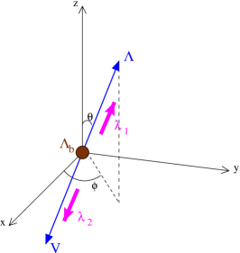
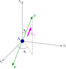
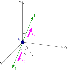
Figure 1: Left-handed: $\Lambda_{b}$ decay in its transversity frame. Right-handed: helicity frames for the $\Lambda$ and vector meson $V$ decays, respectively.

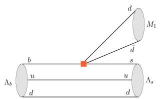
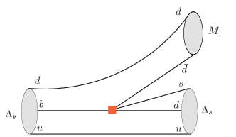
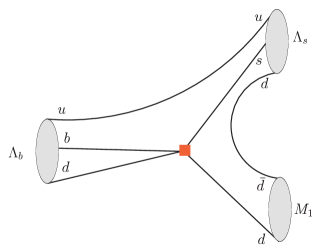
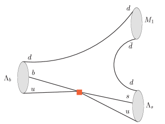
Figure 2: From left-up to right-down, tree (T), color-commensurate (C), exchange (E) and bow tie (B) diagrams which are allowed in transition $\Lambda_{b}\to\Lambda M_{1}.$ The squared dot represents the electroweak interaction in the Standard Model. It can be shown that the contribution of each diagram to the total amplitude follows $T\gg C\approx E\gg B$.

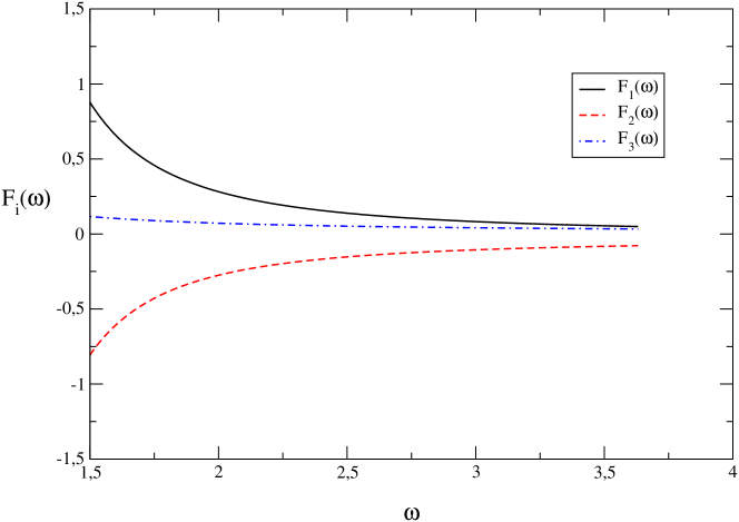
Figure 3: Form factor distributions, $F_{i}(\omega)$, for $\Lambda_{b}\to\Lambda V$. The full, dashed and dot-dashed lines represent $F_{1}(\omega),F_{2}(\omega)$ and $F_{3}(\omega)$, respectively.

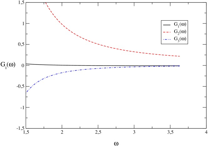
Figure 4: Form factor distributions, $G_{i}(\omega)$, for $\Lambda_{b}\to\Lambda V$. The full, dashed and dot-dashed lines represent $G_{1}(\omega),G_{2}(\omega)$ and $G_{3}(\omega)$, respectively.

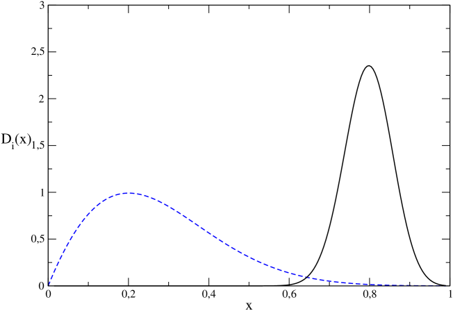
Figure 5: Baryon function distributions for $\Lambda_{b}$ and $\Lambda$. The full and dashed lines represent the $\Lambda_{b}$ and $\Lambda$ distributions, respectively.

Figure 6: Form factor distributions, $\zeta_{i}(\omega)$, for $\Lambda_{b}\to\Lambda V$. The full and dashed lines represent $\zeta_{1}(\omega)$ and $\zeta_{2}(\omega)$ respectively.

Figure 7: Branching ratio asymmetry, $a_{CP}(\omega)$, as a function of the ${\pi}^{+}{\pi}^{-}$ invariant mass in case of $\Lambda_{b}\to\Lambda\rho^{0}(\omega)\to\Lambda\pi^{+}\pi^{-}$ and for $N_{c}^{eff}=3$.

Figure 8: $\cos\theta_{\Lambda}$ (left) and $\phi_{\Lambda}$ (right) distributions of the $\Lambda$-baryon in $\Lambda_{b}$ rest-frame, in case of $\Lambda_{b}\to\Lambda\rho^{0}(\omega)$. The $Y$ axis means $\frac{dN}{d\cos\theta_{\Lambda}}$ (left) and $\frac{dN}{d\phi_{\Lambda}}$ (right).

Figure 9: $\cos\theta_{P}$ (left) and $\phi_{P}$ (right) distributions of the proton in $\Lambda$ rest-frame in case of $\Lambda_{b}\to\Lambda\rho^{0}(\omega)$. The $Y$ axis means $\frac{dN}{d\cos\theta_{P}}$ (left) and $\frac{dN}{d\phi_{P}}$ (right).

Figure 10: $\cos\theta_{\pi}$ (left) and $\cos\theta_{\mu}$ (right) distributions in vector rest-frame, for $\Lambda_{b}\to\Lambda\rho^{0}(\omega)\to\Lambda\pi^{+}\pi^{-}$ and $\Lambda_{b}\to\Lambda J/\psi\to\Lambda\mu^{+}\mu^{-}$, respectively. The $Y$ axis means $\frac{dN}{d\cos\theta_{\pi}}$ (left) and $\frac{dN}{d\phi_{\mu}}$ (right).

Observable	Parity	TR
$\vec{s}$	Even	Odd
$\vec{\cal P}$	Even	Odd
$\vec{e_{Z}}$	Even	Even
$\vec{e_{L}}$	Odd	Odd
$\vec{e_{T}}$	Odd	Odd
$\vec{e_{N}}$	Even	Even
${P_{L}}$	Odd	Even
${P_{T}}$	Odd	Even
${P_{N}}$	Even	ODD

Table 1: Vector-polarization under Parity and TR operations.

$C_{i}^{\prime}$	$q^{2}/m_{b}^{2}=0.3$	$q^{2}/m_{b}^{2}=0.5$
$C_{1}^{\prime}$	$-0.3125$	$-0.3125$
$C_{2}^{\prime}$	$+1.1502$	$+1.1502$
$C_{3}^{\prime}$	$+2.433\times 10^{-2}+1.543\times 10^{-3}i$	$+2.120\times 10^{-2}+2.174\times 10^{-3}i$
$C_{4}^{\prime}$	$-5.808\times 10^{-2}-4.628\times 10^{-3}i$	$-4.869\times 10^{-2}-1.552\times 10^{-2}i$
$C_{5}^{\prime}$	$+1.733\times 10^{-2}+1.543\times 10^{-3}i$	$+1.420\times 10^{-2}+5.174\times 10^{-3}i$
$C_{6}^{\prime}$	$-6.668\times 10^{-2}-4.628\times 10^{-3}i$	$-5.729\times 10^{-2}-1.552\times 10^{-2}i$
$C_{7}^{\prime}$	$-1.435\times 10^{-4}-2.963\times 10^{-5}i$	$-8.340\times 10^{-5}-9.938\times 10^{-5}i$
$C_{8}^{\prime}$	$+3.839\times 10^{-4}$	$+3.839\times 10^{-4}$
$C_{9}^{\prime}$	$-1.023\times 10^{-2}-2.963\times 10^{-5}i$	$-1.017\times 10^{-2}-9.938\times 10^{-5}i$
$C_{10}^{\prime}$	$+1.959\times 10^{-3}$	$+1.959\times 10^{-3}$

Table 2: Wilson coefficients related to current-current tree and penguin operators.

${N_{c}}^{eff}$	$2.0$	$2.5$	$3.0$	$3.5$
$\langle\mathcal{BR}\rangle\;(10^{-7})$	$2.10$	$1.98$	$2.15$	$2.40$
$\langle a_{CP}\rangle$	$6.4\%$	$1.04\%$	$-0.3\%$	$-0.2\%$
$a_{CP}(\omega)$	$96\%$	$15.0\%$	$-7.5\%$	$-3.3\%$

Table 3: Branching ratio, $\mathcal{BR}$, and direct $CP$ violating asymmetry parameters, $a_{CP}$ (mean value) and $a_{CP}(\omega)$ (maximum value), for $\Lambda_{b}\to\Lambda\rho^{0}(\omega)$.

References

- [1] Z. J. Ajaltouni, E. Conte, and O. Leitner, Phys. Lett. B614, 165 (2005), hep-ph/0412116.
- [2] Particle Data Group, S. Eidelman et al., Phys. Lett. B592, 1 (2004).
- [3] B. Andersson, The LUND Model, Cambridge Monographs on Particle Physics (1998).
- [4] M. Jacob and G. C. Wick, Annals of Physics 7, 404 (1959).
- [5] L. Ballentine, Quantum Mechanics: A Modern Development, Singapore World Sci. (1998).
- [6] J. Werle, Relativistic Theory of Reactions, North-Holland Publishing Company- AMSTERDAM , 419 (1966).
- [7] J. Jackson, Resonance Decays, High Energy Physics, Les Houches lectures, edited by C. DeWitt and M. Jacob (Gordon and Breach, New York, 1966 (1965).
- [8] J. G. Korner, M. Kramer, and D. Pirjol, Prog. Part. Nucl. Phys. 33, 787 (1994), hep-ph/9406359.
- [9] F. Hussain and G. Thompson, (1994), hep-ph/9502241.
- [10] M. Neubert, Phys. Rept. 245, 259 (1994), hep-ph/9306320.
- [11] X.-H. Guo, T. Huang, and Z.-H. Li, Phys. Rev. D53, 4946 (1996), hep-ph/9706402.
- [12] A. Datta, Phys. Lett. B349, 348 (1995), hep-ph/9411306.
- [13] B. Konig, J. G. Korner, M. Kramer, and P. Kroll, Phys. Rev. D56, 4282 (1997), hep-ph/9701212.
- [14] C.-S. Huang and H.-G. Yan, Phys. Rev. D59, 114022 (1999), hep-ph/9811303.
- [15] A. J. Buras, Lect. Notes Phys. 558, 65 (2000), hep-ph/9901409.
- [16] A. J. Buras, (1998), hep-ph/9806471.
- [17] G. Buchalla, A. J. Buras, and M. E. Lautenbacher, Rev. Mod. Phys. 68, 1125 (1996), hep-ph/9512380.
- [18] N. G. Deshpande and X.-G. He, Phys. Rev. Lett. 74, 26 (1995), hep-ph/9408404.
- [19] R. Fleischer, Z. Phys. C62, 81 (1994).
- [20] R. Fleischer, Z. Phys. C58, 483 (1993).
- [21] R. Fleischer, Int. J. Mod. Phys. A12, 2459 (1997), hep-ph/9612446.
- [22] G. Kramer, W. F. Palmer, and H. Simma, Nucl. Phys. B428, 77 (1994), hep-ph/9402227.
- [23] R. Enomoto and M. Tanabashi, Phys. Lett. B386, 413 (1996), hep-ph/9606217.
- [24] S. Gardner, H. B. O’Connell, and A. W. Thomas, Phys. Rev. Lett. 80, 1834 (1998), hep-ph/9705453.
- [25] X. H. Guo and A. W. Thomas, Phys. Rev. D58, 096013 (1998), hep-ph/9805332.
- [26] X. H. Guo and A. W. Thomas, Phys. Rev. D61, 116009 (2000), hep-ph/9907370.
- [27] S. Gardner, (1998), hep-ph/9809479.
- [28] S. Gardner, H. B. O’Connell, and A. W. Thomas, (1997), hep-ph/9707414.
- [29] J. J. Sakurai, Currents and Mesons, University of Chicago Press (1969).
- [30] H. B. O’Connell, B. C. Pearce, A. W. Thomas, and A. G. Williams, Prog. Part. Nucl. Phys. 39, 201 (1997), hep-ph/9501251.
- [31] H. B. O’Connell, A. G. Williams, M. Bracco, and G. Krein, Phys. Lett. B370, 12 (1996), hep-ph/9510425.
- [32] H. B. O’Connell, B. C. Pearce, A. W. Thomas, and A. G. Williams, Phys. Lett. B336, 1 (1994), hep-ph/9405273.
- [33] K. Maltman, H. B. O’Connell, and A. G. Williams, Phys. Lett. B376, 19 (1996), hep-ph/9601309.
- [34] H. B. O’Connell, A. W. Thomas, and A. G. Williams, Nucl. Phys. A623, 559 (1997), hep-ph/9703248.
- [35] A. G. Williams, H. B. O’Connell, and A. W. Thomas, Nucl. Phys. A629, 464c (1998), hep-ph/9707253.
- [36] S. Gardner and H. B. O’Connell, Phys. Rev. D59, 076002 (1999), hep-ph/9809224.
- [37] S. Gardner and H. B. O’Connell, Phys. Rev. D57, 2716 (1998), hep-ph/9707385.
- [38] L. Wolfenstein, Phys. Rev. Lett. 51, 1945 (1983).
- [39] L. Wolfenstein, Phys. Rev. Lett. 13, 562 (1964).
- [40] A. Hocker, H. Lacker, S. Laplace, and F. Le Diberder, Eur. Phys. J. C21, 225 (2001), hep-ph/0104062.
- [41] L.-L. Chau and W.-Y. Keung, Phys. Rev. Lett. 53, 1802 (1984).
- [42] S. Pakvasa, S. P. Rosen, and S. F. Tuan, Phys. Rev. D42, 3746 (1990).
- [43] J. D. Jackson, Nuovo Cim. 34, 1644 (1964).
- [44] N. Byers, Spin and Density Matrix of decaying states , CERN 67 20, hep-ph/0412116.
- [45] W. Bensalem, A. Datta, and D. London, Phys. Lett. B538, 309 (2002), hep-ph/0205009.
- [46] T. M. Aliev, V. Bashiry, and M. Savci, Eur. Phys. J. C38, 283 (2004), hep-ph/0409275.
- [47] C. C. et al, Nucl.Phys.B(Proc Suppl) 115, 263 (2003), hep-ph/0210067.
- [48] L. M. Sehgal and J. van Leusen, Phys. Rev. Lett. 83, 4933 (1999), hep-ph/9908426.
- [49] L. Wolfenstein, Phys. Rev. Lett. 83, 911 (1999).
- [50] A. Kadeer, J. G. Korner, and U. Moosbrugger, (2005), hep-ph/0511019.
- [51] D. Binosi and L. Theussl, Comput. Phys. Commun. 161, 76 (2004), hep-ph/0309015.