WUE-ITP-2006-002
Bosonic corrections to the effective leptonic weak mixing angle at the two-loop level

Abstract

Details of the recent calculation of the two-loop bosonic corrections to the effective leptonic weak mixing angle are presented. In particular, the expansion in the difference of the W and Z boson masses is studied and some of the master integrals needed are given in analytic form.

1 INTRODUCTION

The effective leptonic weak mixing angle, $\sin^{2}\theta^{\mbox{\footnotesize lept}}_{\mbox{\footnotesize eff}}$ , is a crucial observable in the indirect determination of the Higgs boson mass from precision experiments up to the Z boson mass scale. Defined through the vertex form factors of the $Z$ at its mass shell

$$\sin^{2}\theta^{\mbox{\footnotesize lept}}_{\mbox{\footnotesize eff}}=\frac{1}{4}\left(1-\Re\left(\frac{g_{V}(M_{Z}^{2})}{g_{A}(M_{Z}^{2})}\right)\right),$$ (1)

it is an UV and IR finite quantity. The current experimental precision requires a careful analysis of the error on the theory side. Here, several contributions have been calculated over the years. In particular, two- and three-loop QCD [1, 2], two-loop electroweak fermionic [3, 4], and parts of the three-loop electroweak contributions [5] are known. Recently, also the Higgs boson mass dependence of the purely bosonic electroweak graphs has been obtained [6]. The computation of the $W$ boson mass from $\mu$ decay, which is part of the final prediction for $\sin^{2}\theta^{\mbox{\footnotesize lept}}_{\mbox{\footnotesize eff}}$ is more complete, since the two-loop electroweak corrections have been fully evaluated [7, 8].

It is important to note, that the prediction from [3] has been used by the LEP Electroweak Working Group for their final report [9]. It is, therefore, necessary, to make sure that the theory error is not underestimated due to the lacking bosonic electroweak corrections. To this end, we have calculated the appropriate diagrams [10] and shown that they fall well within our estimates. It is the purpose of this work to present the details of our computation.

2 MASS DIFFERENCE EXPANSION

The most complicated bosonic diagrams needed for $\sin^{2}\theta^{\mbox{\footnotesize lept}}_{\mbox{\footnotesize eff}}$ are two-loop vertices with up to three different masses, $M_{W}$ , $M_{Z}$ and $M_{H}$. It is only natural [11] to exploit the small difference between $M_{W}$ and $M_{Z}$ to reduce the number of scales. Furthermore, since the authors of [6] have evaluated the Higgs boson mass dependence of the result normalized at $M_{H}$ = 100 GeV, it is only necessary to evaluate the graphs at the same point at first (of course an independent check of the mass dependence is also required). This allows a further mass difference expansion, with expansion parameter $s^{2}_{H}=1-M^{2}_{H}/M^{2}_{Z}$ .

It is clear that if there are thresholds at $M_{W}=M_{Z}$, then starting from some order in the expansion in $s^{2}_{W}=1-M^{2}_{W}/M^{2}_{Z}$, we are going to encounter divergences. A suitable technique to recover the correct value is the expansion by regions method [12]. The idea is to analyze the momentum regions, which can contribute to the integral,and expand the integrand in each region suitably performing the integration in dimensional regularization. In the case, when only one line can go on-threshold, there are just two regions: ultrasoft, (us), where $k_{1,2}\sim s^{2}_{W}M_{Z}$; and hard, (h), where $k_{1,2}\sim M_{Z}$. The classification of the size of the momenta has to be supplied by a momentum routing, which clearly needs to be such that the selected line goes on-threshold when $s_{W}=0$.

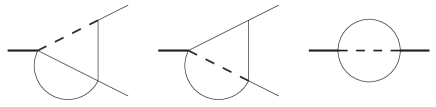
$I_{1}$                      $I_{2}$                      $I_{3}$

Figure 1: Ultrasoft graphs in the mass difference expansion. Dashed lines go on-threshold, when $M_{W}=M_{Z}$, and thin solid lines are massless.

In the (us) region, one encounters three possible topologies, Fig. 1. The expansion transforms a Feynman integral into an unusual form, since

$$\frac{1}{(k_{1,2}-p)^{2}-M_{W}^{2}}\sim\frac{1}{-2k_{1,2}p+s_{W}^{2}M_{Z}^{2}},$$ (2)

and

$$\frac{1}{(k_{1,2}-p_{1,2})^{2}}\sim\frac{1}{-2k_{1,2}p_{1,2}}.$$ (3)

The last integral in Fig. 1, $I_{3}$, with the above substitutions (actually just Eq. (2)) has been evaluated in [12]. The other two turn out to be reducible by the integration-by-parts technique to the last case. In practice this exercise has been left to IdSolver [13], with the result

$$I_{1}=\frac{1}{s_{W}^{2}M_{Z}^{2}}\frac{4\epsilon-3}{1-2\epsilon}I_{3},$$ (4)

and

$$I_{2}=\frac{1}{s_{W}^{2}M_{Z}^{2}}\left(\frac{3}{\epsilon}-4\right)I_{3},$$ (5)

where

$$I_{3} = \left(i\pi^{d/2}e^{-\epsilon\gamma_{E}}\right)^{2}\Gamma^{2}(1-\epsilon)\Gamma(4\epsilon-3)$$

$$\times (M_{Z}^{2})^{1-2\epsilon}(-s_{W}^{2})^{3-4\epsilon}.$$

Since there is no problem with the evaluation of the master integrals, the rest of the calculation has been reduced to the application of IdSolver to all integrals with numerators and dots.

3 MASTER INTEGRALS

The integrals in the hard momentum region,(h), have the usual Feynman integrand structure, with some propagators on-threshold. In practice this means that each one of them is given by a series in $\epsilon$ with numeric coefficients multiplied by a trivial scaling factor. The problem is now that we have spurious poles in the reduction to master integrals and we need analytic results for constant parts of some nontrivial integrals in order to check the exact cancellation of divergences. Of course, one could think of constructing an $\epsilon$-finite basis in the sense of [14], but we would in the end have to evaluate integrals with collinear singularities (even though just to finite parts). Therefore we tried to find a basis that would produce a relatively small number of spurious poles, but in front of simple integrals.

Indeed, there are 73 master integrals, 1 needed to ${\cal O}(\epsilon^{3})$, 6 to ${\cal O}(\epsilon^{2})$, and 26 to ${\cal O}(\epsilon)$. Most of the integrals needed to high orders in the $\epsilon$-expansion could be found in the literature. In particular, several vertex integrals have been given in [15]. However, 7 integrals remained to be evaluated analytically down to the finite part, Fig. 2. To this end, we used series representations in the small external momentum regime, which were subsequently improved with the help of conformally mapped Padé approximants, and resummed empirically with the PSLQ algorithm. The expansions were derived from Mellin-Barnes representations and analyzed with the help of the MB package [16]. With the usual $\overline{\mbox{MS}}$ normalization of the momentum integrations, i.e. $e^{\epsilon\gamma_{E}}/i\pi^{d/2}\int d^{d}k$ per loop, the results are

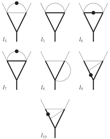
Figure 2: Some hard momentum region graphs needed to ${\cal O}(\epsilon)$. Thick lines are massive and on-shell, whereas thin are massless. A dot represents a squared propagator.

$$I_{4} = \frac{\pi^{2}}{9\epsilon}+\frac{3\pi\mbox{S2}}{\sqrt{3}}-\frac{2}{9}\zeta_{3},$$ (7)

$$I_{5} = \frac{1}{2\epsilon^{2}}+\frac{1}{\epsilon}\left(\frac{5}{2}-\frac{\pi}{\sqrt{3}}\right)+\frac{19}{2}+\frac{\pi^{2}}{18}$$

$$- \frac{9\mbox{S2}}{4}-\frac{5\pi}{\sqrt{3}}+\frac{\pi\log 3}{\sqrt{3}}+\frac{9\pi\mbox{S2}}{2\sqrt{3}}-\frac{8}{3}\zeta_{3},$$

$$I_{6} = \frac{9\pi\mbox{S2}}{2\sqrt{3}}-\frac{8}{3}\zeta_{3},$$

$$I_{7} = \frac{\pi^{2}}{18\epsilon}-\frac{15\pi\mbox{S2}}{2\sqrt{3}}+\frac{23}{9}\zeta_{3},$$

$$I_{8} = \frac{1}{2\epsilon^{2}}+\frac{3}{2\epsilon}+\frac{5}{2}+\frac{\pi^{2}}{36}+\frac{\pi}{\sqrt{3}}-\frac{9\pi\mbox{S2}}{2\sqrt{3}}+\frac{1}{3}\zeta_{3},$$

$$I_{9} = -\frac{\pi^{3}}{54\sqrt{3}}+\frac{3\pi\mbox{S2}}{2\sqrt{3}}+\frac{2}{9}\zeta_{3},$$

$$I_{10} = \frac{3\pi\mbox{S2}}{\sqrt{3}}-\frac{5}{9}\zeta_{3},$$

where S2 = $4/(9\sqrt{3})\mbox{Cl}_{2}(\pi/3)$, with $\mbox{Cl}_{2}(x)=\Im(\mbox{Li}_{2}(e^{ix}))$, and the mass has been set to unity.The ${\cal O}(\epsilon)$ parts of these integrals and finite parts of the remaining ones have been evaluated numerically, either from small momentum expansions,or from integral representations. There was no need to invest into an analytic result.

During the reduction of the integrals to masters, and in particular of a four line propagator, an interesting relation has been discovered, Fig. 3. Such a relation could certainly not be found during the reduction of the three line propagator graph, since the vacuum graph has the same number of lines, but a different mass and momentum distribution. In fact, reducing the propagator leads to the two masters, the dotted and the undotted. This result demonstrates that the integration-by-parts relations do not exhaust all the rational function coefficient linear relations between integrals with a fixed upper number of lines in general.

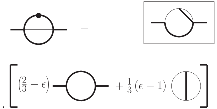
Figure 3: Exact relation between 3-line masters on-shell. The integral, of which IBPs contain this relation is shown in the frame.

Note, that the fact that there is a simple relation between the two 3-line propagator master integrals has been known since [17], but there,it was not identified as a relation between three integrals.

4 VERTEX CONTRIBUTIONS

Summing up all of the vertex contributions in Feynman gauge, with the mass parameter of dimensional regularization set to $M_{Z}$, and $M_{H}$ = 100 GeV, one obtains

$$\!\!\!\!\!-4.4\times 10^{-6}\frac{1}{s^{2}_{W}}(1-1.1s^{2}_{W}-3.9s^{4}_{W}-0.8s^{6}_{W}$$

$$+0.2s^{8}_{W}+1.1\times 10^{-3}\log(s^{2}_{W})s^{8}_{W}+...)$$ (8)

Even though just part of the calculation, this formula is interesting by itself. First of all, the remaining part of the result can be evaluated to very high precision for any masses, since it is expressed by at most two-loop propagators, and therefore, the above series determines the final precision. Second, Eq. (4) proves that one should resist the temptation to approximate the final contribution by the leading term, which is relatively easily evaluated by setting $M_{W}=M_{Z}$ in all lines. In fact, because $s^{2}_{W}\simeq 1/4$, the sum of the first three terms is equal to half of the leading one. Finally, the ultrasoft contribution connected to the logarithm of $s_{W}$ starts very late in the expansion and has a small coefficient, which means that one could have obtained a reliable approximation without the strategy of regions.

Figure 4: Behavior of the subsequent terms of the expansion in $s_{H}^{2}$ of the sum of the vertex graphs.

The convergence of the expansion can also be studied by looking at the dependence on $M_{H}$.The first five terms of the expansion are

$$\!\!\!\!\!-1.1\times 10^{-5}(1+0.13s^{2}_{H}+0.04s^{4}_{H}+0.02s^{6}_{H}+0.01s^{8}_{H}),$$

which shows nice convergence at $M_{H}=0$, corresponding to $s^{2}_{H}=1$. At the other end of the scale we obtain an alternating series, which strongly diverges even below the threshold for Higgs boson decay into a pair of gauge bosons, as shown in Fig. 4. It turns out that this behavior can be of advantage. In particular, being alternating this series should lend itself nicely to Padé resummation techniques, closing the gap between the mass difference and large Higgs boson mass expansion. A similar phenomenon has been observed during the computation of the bosonic corrections to $\mu$ decay [8].

5 SUMMARY

We have discussed computational techniques used in the recent computation of the complete bosonic contributions to the effective leptonic weak mixing angle. As a by product, we have presented new results for on-shell two-loop vertices and a relation between on-shell propagator master integrals.

6 ACKNOWLEDGMENT

M.C. would like to thank M. Yu. Kalmykov for drawing his attention to [17].

References

- [1] A. Djouadi and C. Verzegnassi, Phys. Lett. B 195 (1987) 265; A. Djouadi, Nuovo Cim. A 100 (1988) 357; B. A. Kniehl, Nucl. Phys. B 347 (1990) 86; F. Halzen and B. A. Kniehl, Nucl. Phys. B 353 (1991) 567; B. A. Kniehl and A. Sirlin, Nucl. Phys. B 371 (1992) 141; Phys. Rev. D 47 (1993) 883; A. Djouadi and P. Gambino, Phys. Rev. D 49 (1994) 3499 [Erratum-ibid. D 53 (1996) 4111].
- [2] K. G. Chetyrkin, J. H. Kühn and M. Steinhauser, Phys. Rev. Lett. 75 (1995) 3394; Nucl. Phys. B 482 (1996) 213.
- [3] M. Awramik, M. Czakon, A. Freitas and G. Weiglein, Phys. Rev. Lett. 93 (2004) 201805.
- [4] W. Hollik, U. Meier and S. Uccirati, Nucl. Phys. B 731 (2005) 213.
- [5] M. Faisst, J. H. Kuhn, T. Seidensticker and O. Veretin, Nucl. Phys. B 665 (2003) 649; R. Boughezal, J. B. Tausk and J. J. van der Bij, Nucl. Phys. B 713 (2005) 278; R. Boughezal, J. B. Tausk and J. J. van der Bij, Nucl. Phys. B 725 (2005) 3.
- [6] W. Hollik, U. Meier and S. Uccirati, Phys. Lett. B 632 (2006) 680.
- [7] A. Freitas, W. Hollik, W. Walter and G. Weiglein, Phys. Lett. B 495 (2000) 338 [Erratum-ibid. B 570 (2003) 260], Nucl. Phys. B 632 (2002) 189 [Erratum-ibid. B 666 (2003) 305]; M. Awramik and M. Czakon, Phys. Lett. B 568 (2003) 48.
- [8] M. Awramik and M. Czakon, Phys. Rev. Lett. 89 (2002) 241801; A. Onishchenko and O. Veretin, Phys. Lett. B 551 (2003) 111; M. Awramik, M. Czakon, A. Onishchenko and O. Veretin, Phys. Rev. D 68 (2003) 053004.
- [9] the LEP Collaborations [OPAL Collaboration], arXiv:hep-ex/0511027.
- [10] M. Awramik, M. Czakon, A. Freitas, in preparation.
- [11] F. Jegerlehner, M. Y. Kalmykov and O. Veretin, Nucl. Phys. B 641 (2002) 285; F. Jegerlehner, M. Y. Kalmykov and O. Veretin, Nucl. Phys. B 658 (2003) 49.
- [12] V. A. Smirnov, “Applied asymptotic expansions in momenta and masses”, Berlin, Germany, Springer (2002).
- [13] M. Czakon, “DiaGen/IdSolver”, unpublished; see also M. Awramik, M. Czakon, A. Freitas and G. Weiglein, Nucl. Phys. Proc. Suppl. 135 (2004) 119.
- [14] K. G. Chetyrkin, M. Faisst, C. Sturm and M. Tentyukov, arXiv:hep-ph/0601165.
- [15] U. Aglietti and R. Bonciani, Nucl. Phys. B 668 (2003) 3; U. Aglietti and R. Bonciani, Nucl. Phys. B 698 (2004) 277.
- [16] M. Czakon, arXiv:hep-ph/0511200.
- [17] A. I. Davydychev and M. Y. Kalmykov, Nucl. Phys. B 605 (2001) 266.