A Markov Chain Monte Carlo Analysis of the CMSSM

Abstract:

We perform a comprehensive exploration of the Constrained MSSM parameter space employing a Markov Chain Monte Carlo technique and a Bayesian analysis. We compute superpartner masses and other collider observables, as well as a cold dark matter abundance, and compare them with experimental data. We include uncertainties arising from theoretical approximations as well as from residual experimental errors of relevant Standard Model parameters. We delineate probability distributions of the CMSSM parameters, the collider and cosmological observables as well as a dark matter direct detection cross section. The 68% probability intervals of the CMSSM parameters are: $0.52\mbox{ TeV}<m_{1/2}<1.26\mbox{ TeV}$, $m_{0}<2.10\mbox{ TeV}$, $-0.34\mbox{ TeV}<A_{0}<2.41\mbox{ TeV}$ and $38.5<\tan\beta<54.6$. Generally, large fractions of high probability ranges of the superpartner masses will be probed at the LHC. For example, we find that the probability of $m_{\widetilde{g}}<2.7\mbox{ TeV}$ is 78%, of $m_{\tilde{q}_{R}}<2.5\mbox{ TeV}$ is 85% and of $m_{\chi_{1}^{\pm}}<0.8\mbox{ TeV}$ is 65%. As regards the other observables, for example at 68% probability we find $3.5\times 10^{-9}<BR(B_{s}\rightarrow\mu^{+}\mu^{-})<1.7\times 10^{-8}$, $1.9\times 10^{-10}<\delta a_{\mu}^{\text{SUSY}}<9.9\times 10^{-10}$ and $1\times 10^{-10}\,\mbox{pb}<\sigma^{SI}_{p}<1\times 10^{-8}\,\mbox{pb}$ for direct WIMP detection. We highlight a complementarity between LHC and WIMP dark matter searches in exploring the CMSSM parameter space. We further expose a number of correlations among the observables, in particular between $BR(B_{s}\rightarrow\mu^{+}\mu^{-})$ and $BR({\bar{B}}\rightarrow X_{s}\gamma)$ or $\sigma^{SI}_{p}$. Once SUSY is discovered, this and other correlations may prove helpful in distinguishing the CMSSM from other supersymmetric models. We investigate the robustness of our results in terms of the assumed ranges of CMSSM parameters and the effect of the $(g-2)_{\mu}$ anomaly which shows some tension with the other observables. We find that the results for $m_{0}$, and the observables which strongly depend on it, are sensitive to our assumptions, while our conclusions for the other variables are robust.

1 Introduction

Two of the most challenging questions facing particle physics today are the instability of the Higgs mass against radiative corrections (known as the “fine–tuning problem”) and the nature of dark matter (DM). Unlike in the Standard Model (SM), both find plausible solutions in the framework of weak scale softly broken supersymmetry (SUSY). Firstly, the fine–tuning problem is addressed via the cancellation of quadratic divergences in the radiative corrections to the Higgs mass. Secondly, assuming $R$–parity, the lightest supersymmetric particle (LSP) is a leading weakly interactive massive particle (WIMP) candidate for cold DM (CDM). On the other hand, despite these and other attractive features, without a reference to grand unified theories (GUTs), low energy SUSY models suffer from the lack of predictivity due to a large number of free parameters (e.g., over 120 in the Minimal Supersymmetric Standard Model (MSSM)), most of which arise from the SUSY breaking sector. At present, experimental constraints on superpartner masses from direct SUSY searches at LEP and the Tevatron remain fairly mild, although a dramatic improvement is expected once the LHC comes into operation in 2007. Indirect limits from bounds on CP–violation and flavor changing neutral currents are generally much stronger (except for the 2nd–3rd generation mixings) but even these can be evaded, for example if SUSY breaking is “universal”.

The MSSM with one particularly popular choice of universal boundary conditions at the grand unification scale is called the Constrained Minimal Supersymmetric Standard Model (CMSSM) [1]. The CMSSM is defined in terms of five free parameters: common scalar ($m_{0}$), gaugino ($m_{1/2}$) and tri–linear ($A_{0}$) mass parameters (all specified at the GUT scale) plus the ratio $\tan\beta$ of Higgs vacuum expectation values and $\text{sign}(\mu)$, where $\mu$ is the Higgs/higgsino mass parameter whose square is computed from the conditions of radiative electroweak symmetry breaking (EWSB). The economy of parameters in this scheme makes it a useful tool for exploring SUSY phenomenology. In addition to experimental limits on Higgs and superpartner masses, and strong bounds on SUSY contributions to $BR({\bar{B}}\rightarrow X_{s}\gamma)$ and the anomalous magnetic moment of the muon $(g-2)_{\mu}$, a very strong constraint limiting the mass parameters of the model from above is provided by the relic abundance of the LSP. Within the CMSSM the neutral LSP is the (bino–like) lightest neutralino [2, 3, 1]. It is well known that recent precise determinations of the relic density $\Omega_{\text{CDM}}h^{2}$ of non–baryonic CDM obtained by combining WMAP data with other observations of cosmic microwave background (CMB) anisotropies and large scale structure data, provide an important and often tight constraint on the CMSSM parameter space.

It is worth remembering that the CMSSM is not the only viable and economical framework providing well defined and strongly constrained ranges of parameters. A virtue of the CMSSM lies in the particularly simple boundary conditions at the unification scale and, as a result, in a minimal number of parameters. A drawback is that the CMSSM, as a framework, is not broad enough to accommodate a richer structure of GUT–scale physics, in particular a non–minimal flavor structure and many realistic fermion family patterns. One attractive and well studied model is the MSSM with boundary conditions at the unification scale imposed by consistency with a minimal $SO(10)$ GUT model [7, 8].

The most popular approach to exploring and delimiting viable regions of the parameter space of the CMSSM and other SUSY models has been a usual method of evaluating the goodness–of–fit of points scanned using fixed grids [9]. Such scans have the advantage of pre–determining the ranges and step size for each parameter and thus of being able to control exactly which points in the parameter space will be probed. On the other hand, the method has several strong limitations. Firstly, the number of points required scales as $k^{N}$, where $N$ is the number of the model’s parameters and $k$ the number of points for each of them. Therefore this approach becomes highly inefficient for exploring with sufficient resolution parameter spaces of even modest dimensionality, say $N>3$. Secondly, narrow “wedges” and similar features of parameter space can easily be missed by not setting a fine enough resolution (which, on the other hand, are likely to be completely unnecessary outside such special regions). Thirdly, extra sources of uncertainties (e.g., those due to the lack of precise knowledge of SM parameter values) and relevant external information (e.g., about the parameter range) are difficult to accommodate.

In contrast, Bayesian statistics formalism linked to a Markov Chain Monte Carlo (MCMC) method of exploring a multi–dimensional parameter space offer several advantages. In the Bayesian context, the required computational power scales very favorably with the dimensionality of parameter space, $N$. The details depend on the problem under consideration, but roughly the number of points needed scales approximately linearly with $N$. Secondly, it is straightforward to include in the analysis all sources of uncertainty that are present in the highly complex problem of comparing theoretical predictions with current collider and cosmological measurements. For instance, our imperfect knowledge of the relevant SM parameters has an impact on our statistical conclusions (i.e., inferences) about the values of the quantities of interest, in our case the CMSSM parameters. This source of uncertainty can fully and easily be accounted for in Bayesian statistics. Thirdly, probability distributions can be computed for any function of the CMSSM parameters, and in particular for all interesting physical observables.

The MCMC approach has been widely used in several branches of science with much success and is gaining popularity in the astrophysics and cosmology community. (For some recent applications, see e.g. [10] for cosmological data analysis, [11] in the astrophysical context, and e.g. [12] for a general introduction to Bayesian methods.) Within the context of softly broken low energy SUSY, limited random (not MCMC) scans were first interpretted in the language of statistical analysis in [13] in the MSSM with diagonal flavor mass entries, and in the CMSSM in [14, 15]. The MCMC method was first applied to the CMSSM in [16] (with some modifications) and more recently in [17, 18].

In the present work, we employ the MCMC algorithm to explore the parameter space of the CMSSM. The model is constrained with data coming from present collider data and cosmological observations of the CDM abundance. We compute the $W$ boson pole mass $M_{W}$, ${\sin^{2}\theta_{\text{eff}}}$, Higgs and superpartner masses, $BR({\bar{B}}\rightarrow X_{s}\gamma)$, the anomalous magnetic moment of the muon $(g-2)_{\mu}$, $BR(B_{s}\rightarrow\mu^{+}\mu^{-})$ and $\Omega_{\chi}h^{2}$, and compare them with current experimental data. We also compute a spin–independent dark matter WIMP elastic scattering cross section on a free proton, $\sigma^{SI}_{p}$, but we do not enforce upper experimental limits because of the uncertainties in the structure of the Galactic halo as well as in the values of some hadronic matrix elements entering the computation of $\sigma^{SI}_{p}$. We shall see that the current experimental limit lies just above the high–probability regions of parameter space.

Our analysis goes beyond other recent works in several aspects. We include both experimental and theoretical uncertainties in treating relevant SM quantities. Instead of applying a sharp cut at experimental limits, we smear them out by incorporating theoretical and experimental uncertainties. Furthermore, we improve the accuracy of CMSSM predictions for the neutralino relic abundance by including previously neglected dependence on the remaining uncertainty in the fine structure constant. Our analysis covers larger values of $m_{0}$ than in [17], thus allowing us to explore the focus point (FP) region [19]. We present inferences on the high probability regions for the CMSSM parameters and superpartner masses, and for the other observables listed above. We emphasize that, in some cases, inferences on the favored intervals of some parameters do depend on the assumed prior ranges, while in the other the inferred high–probability regions are fairly robust. As we will see, this often affects resulting conclusions about prospects for SUSY discovery at the LHC or in DM searches. We point out the difference between posterior probability (Bayesian statistics) and the quality–of–fit statistics, and emphasize that a discrepancy between the two methods can be only resolved with better data.

The paper is organized as follows. In section 2 we briefly review some elements of Bayesian statistics and the MCMC method, and introduce our 8–dimensional parameter space which we explore in the following. In section 3 we describe the current collider and astrophysical data used in the analysis to put constraints on the CMSSM. We present and discuss our results in section 4. In section 5 we summarize our main findings and conclusions.

2 Bayesian statistics and the CMSSM

In this section we introduce some basic concepts of the Bayesian statistics and apply them to the CMSSM.

2.1 Parameters and probabilities

We are interested in delineating high probability regions of the CMSSM parameter space. We fix $\text{sign}(\mu)=+1$ throughout (see below) and denote the remaining four free CMSSM parameters by the set

$$\theta=(m_{0},m_{1/2},A_{0},\tan\beta).$$ (1)

In most of previous analyses, the values of the SM parameters, such as the top quark mass, which strongly influences some of the CMSSM predictions, have been fixed at their central values. However, the statistical uncertainty associated with our imperfect knowledge of the values of relevant SM parameters must be taken into account in order to obtain correct statistical conclusions on the regions of high probability for the CMSSM parameters. This can easily be done in a Bayesian framework by introducing a set $\psi$ of so–called “nuisance parameters”. For the purpose of this analysis the most relevant ones are

$$\psi=(M_{t},m_{b}(m_{b})^{\overline{MS}},\alpha_{\text{em}}(M_{Z})^{\overline{MS}},\alpha_{s}(M_{Z})^{\overline{MS}}),$$ (2)

where $M_{t}$ is the pole top quark mass, $m_{b}(m_{b})^{\overline{MS}}$ is the bottom quark mass at $m_{b}$, while $\alpha_{\text{em}}(M_{Z})^{\overline{MS}}$ and $\alpha_{s}(M_{Z})^{\overline{MS}}$ are the electromagnetic and the strong coupling constants at the $Z$ pole mass $M_{Z}$. The last three parameters are evaluated in the $\overline{MS}$ scheme.

The set of parameters $\theta$ and $\psi$ form an 8–dimensional set $\eta$ of our “basis parameters”

$$\eta=(\theta,\psi).$$ (3)

In the following, we shall specify a set $\xi$ of several collider and cosmological observables which we call “derived variables”,

$$\xi=(\xi_{1},\xi_{2},\ldots,\xi_{m}).$$ (4)

Their values depend on the CMSSM and SM parameters $\eta$ sampled in our MCMC analysis, $\xi(\eta)$. Some of the observables will be used to compare CMSSM predictions with experimental set of data $d$ which is currently available either in the form of positive measurements or as limits.

The central quantity which constitutes the basis of all probabilistic inferences is the posterior probability density function (pdf) $p(\eta|d)$ for the basis parameters $\eta$. The posterior pdf represents our state of knowledge about the parameters $\eta$ after we have taken the data into consideration (hence the name). Using Bayes’ theorem, the posterior pdf is given by

$$p(\eta|d)=\frac{p(d|\xi)\pi(\eta)}{p(d)}.$$ (5)

On the rhs of Eq. (5), the quantity $p(d|\xi)$, taken as a function of $d$ for a given $\eta$, and hence a given $\xi(\eta)$, is called a “sampling distribution”. It represents the probability of reproducing the data $d$ for a fixed value of $\xi(\eta)$. Considered instead as a function of $\xi$ for fixed data $d$, $p(d|\xi)$ is called the likelihood (where the dependence of $\xi$ on $\eta$ is understood). The likelihood supplies the information provided by the data. In section 3.1 we explain in detail how it is constructed in our analysis. The quantity $\pi(\eta)$ denotes a prior probability density function (hereafter called simply a prior) which encodes our state of knowledge about the values of the parameters in $\eta$ before we see the data. The state of knowledge is then updated to the posterior via the likelihood. Finally, the quantity in the denominator is called evidence or model likelihood. In the context of this analysis it is only a normalization constant, independent of $\eta$, and therefore will be dropped in the following. For further details about the terminology of Bayesian statistics, see e.g., [20, 12].

Since in this work we are not interested in the nuisance parameters $\psi$ themselves, at the end we simply marginalize over them by integrating $p(\eta|d)$ over their values. This procedure gives a posterior pdf for the interesting CMSSM parameters $\theta$ which takes full account of the uncertainties in $\psi$

$$p(\theta|d)=\int p(\theta,\psi|d)\,d^{4}\psi.$$ (6)

Note that all pdf’s should normally be normalized so that the total probability is unity. However, for the parameter estimation procedure presented here only the relative posterior pdf’s are relevant, and in the following we shall plot pdf’s normalized in such a way that their maximum value is one. In practice, we will present pdf’s for only one or two variables at the time, with the remaining ones integrated over. We will introduce and discuss several of them in Section 4 where we present our results.

The purpose of the MCMC exploration of parameter space is to obtain a series of points (called a “chain”), whose density distribution is proportional to the posterior pdf on the rhs of Eq. (5). Further details about the MCMC procedure are given in appendix A. From the samples in the chain, it is straightforward to obtain all pdf’s of interest by plotting histograms of the number of samples as a function of the parameter values that one wants to examine. In particular, one does not need to carry out the marginalization integral in Eq. (6) explicitly. It is sufficient to ignore the coordinates of the samples in parameter space along the marginalized directions. This is one more major advantage of the MCMC method.

Another useful feature is that from the posterior pdf $p(\eta|d)$ we can obtain the posterior pdf for any function $f$ of basis parameters, using the fact that

$$p(f,\eta|d)=p(f|\eta,d)p(\eta|d)=\delta(f(\eta)-f)p(\eta|d),$$ (7)

where $\delta(x)$ denotes the delta–function. Therefore for every sample in the MC chain, one simply computes $f(\eta$) and the resulting density of points in the $(f,\eta)$ space is proportional to the posterior pdf $p(f,\eta|d)$. From this pdf one can then obtain by marginalization the pdf for any subset of $(f,\eta)$. In particular, if we take $f(\eta)=\xi(\eta)$, we can then investigate probability distributions for any combination of the basis and the derived parameters, as well as their correlations. This is investigated in section 4.

Before we can proceed to delineating high probability regions in the CMSSM parameter space, first we must choose our priors and specify the likelihood. This is the subject of the next two sections.

2.2 The choice of prior probabilities

It is clear from the rhs of Eq. (5) that in the Bayesian approach the first step is to specify the functional form of the prior pdf. This is equivalent to assigning a probability measure to parameter space. The principle of indifference states that one should assign equal probabilities to equal states of knowledge before seeing the data. In our case, the basis parameters are location parameters over which it is appropriate to set a flat prior

$$\pi(\eta)=\left\{\begin{array}[]{l l}\begin{aligned} &\text{const}\quad&\text{ for }\eta_{\text{min}}<\eta<\eta_{\text{max}}\\ &0&\text{otherwise},\end{aligned}\end{array}\right.$$ (8)

where the constant is determined by the requirement that the prior integrates to probability one. Since we assume no correlation of priors between the SM and the CMSSM parameters, the joint prior can be written as

$$\pi(\eta)=\pi(\theta)\pi(\psi).$$ (9)

Flat priors are thus characterized by their ranges $[\eta_{\text{min}},\eta_{\text{max}}]$. One alternative possibility would be to employ a “naturalness” prior which gives more weight to points exhibiting less fine–tuning [18].

CMSSM parameters $\theta$
“2 TeV  range”	“4 TeV  range”
$50\mbox{ GeV}<m_{0}<2\mbox{ TeV}$	$50\mbox{ GeV}<m_{0}<4\mbox{ TeV}$
$50\mbox{ GeV}<m_{1/2}<2\mbox{ TeV}$	$50\mbox{ GeV}<m_{1/2}<4\mbox{ TeV}$
$|A_{0}|<5\mbox{ TeV}$	$|A_{0}|<7\mbox{ TeV}$
$2<\tan\beta<62$
SM (nuisance) parameters $\psi$
$160\mbox{ GeV}<M_{t}<190\mbox{ GeV}$
$4\mbox{ GeV}<m_{b}(m_{b})^{\overline{MS}}<5\mbox{ GeV}$
$127.5<1/\alpha_{\text{em}}(M_{Z})^{\overline{MS}}<128.5$
$0.10<\alpha_{s}(M_{Z})^{\overline{MS}}<0.13$

Table 1: Initial ranges for our basis parameters $\eta=(\theta,\psi)$, with flat prior probability distributions assumed.

Our SUSY and SM parameter priors are summarized in Table 1. In this work we consider two initial ranges of CMSSM parameters. In one, which we call a “2 TeV range”, we assume $50\mbox{ GeV}<m_{0},m_{1/2}<2\mbox{ TeV}$ and $|A_{0}|<5\mbox{ TeV}$. This choice is motivated by an expected LHC reach in exploring superpartner mass and by a general “naturalness” argument of SUSY mass parameters to preferably lie within $\mathcal{O}(1\mbox{ TeV})$. In the other case, called a “4 TeV range”, we assume $50\mbox{ GeV}<m_{0},m_{1/2}<4\mbox{ TeV}$ and $|A_{0}|<7\mbox{ TeV}$, which goes far beyond the LHC reach. (The larger range will include the focus point region, along with various uncertainties involved. We will discuss this point later.) We will compare our findings for both ranges in order to see to what extent statistical conclusions depend on our preconceived expectation that a SUSY signal might lie within reach of the LHC (represented by the “2 TeV range”). Such a sensitivity test is essential to establish the extent to which inferences depend on the initial range one chooses, i.e. on the prior. The lower bounds on $m_{0}$ and $m_{1/2}$ come from the negative results of sparticle searches. We allow a rather generous range for $A_{0}$, in part to see to what extent this choice would allow one to reduce [21] the impact of the cosmological constraint, which in the usually explored case of $A_{0}=0$ is very tight. For both sets we further assume $2<\tan\beta<62$. The lower bound comes from negative Higgs searches [22]. Very large values of $\tan\beta\mathrel{\hbox to0.0pt{\lower 4.0pt\hbox{\hskip 1.0pt$\sim$}\hss}\raise 1.0pt\hbox{$>$}}60$ are in conflict with theoretical considerations, e.g. they would make it extremely difficult to achieve radiative electroweak symmetry breaking [23]. Furthermore, at such large $\tan\beta$ large uncertainties arise in the computation of the SUSY spectrum, leading to unreliable predictions. On the other hand, since the SM nuisance parameters are well measured, it turns out that their prior ranges are irrelevant for the outcome of the analysis.

Before closing this section, we comment that the necessity of choosing priors is often (incorrectly) regarded as a limitation to the “objectivity” of the Bayesian approach. This can be easily dispelled by noting that two scientists in the same state of knowledge before seeing the data (i.e., who have assumed the same priors) will necessarily reach the same conclusions. When the choice of priors makes a difference in drawing the final inference (given by the posterior pdf), this is a “health warning” that the data is not informative enough, e.g. the likelihood is not sufficiently peaked to override the assumed prior distribution. In this case, the inference on the parameters must rely either on external relevant information in the form of the prior (e.g., a theoretical “naturalness criterion” investigated in Ref. [18]), or of better and more constraining data. In the present study, this will be the case for the parameter $m_{0}$, as we discuss in section 4.1.

3 Collider and cosmological observables

In this section, we first define the likelihood function for the CMSSM. Next, we introduce the data that we use for the nuisance parameters, and then proceed to describe electroweak and dark matter observables. We give details about their calculation, the theoretical uncertainties involved and the experimental errors in their determination.

3.1 Constructing the likelihood for the CMSSM

The likelihood is a key element of our analysis. It encodes the information from the observational data and therefore particular care must be taken in constructing it. In the Bayesian framework it would be easy to incorporate the full likelihood functions from various experimental measurements if they were available. However, even though the actual measurements contain much more useful information, most measurements in particle physics experiments are presented only by the mean and the standard deviation, while upper or lower exclusion bounds are usually given in terms of the $95\%$ exclusion CL.

Uncertainties in the observable quantities can be split into two categories. The first is an experimental uncertainty, the second is a theoretical one and is a consequence of making some approximations (e.g., neglecting higher order loop corrections), a limited numerical precision in the code, etc. In practice, the theoretical uncertainty can be modelled in a Bayesian context by considering that our mapping from the basis parameters $\eta$ to the derived quantities $\xi$ is imperfect: instead of an “exact” mapping $\hat{\xi}(\eta)$ we actually have only an imperfect version $\xi(\eta)$ which suffers from the sort of uncertainties outlined above. The likelihood $p(d|\xi)$ introduced in Eq. (5) can then be written as

$$p(d|\xi)=\int p(d|\hat{\xi})p(\hat{\xi}|\xi)d^{m}\hat{\xi},$$ (10)

where we have integrated out the true (and unknown) mapping. The pdf $p(\hat{\xi}|\xi)$ encodes the estimated uncertainty of our mapping. Usually we only have (at best) an estimate of the theoretical errors, which means that we only have information on the scale of the associated uncertainty. This is described by a multi–normal distribution of a general form

$$p(\hat{\xi}|\xi)=\frac{1}{(2\pi)^{m/2}|C|^{1/2}}\exp\left(-\frac{1}{2}(\xi-\hat{\xi})C^{-1}(\xi-\hat{\xi})^{T}\right),$$ (11)

where $C$ is an $m\times m$ covariance matrix describing the error of the mapping ($m$ being the number of elements in $\xi$) and $|C|$ denotes its determinant. If one assumes that the theoretical errors $\tau_{i}$ ($i=1,\ldots,m$) for the different quantities are uncorrelated then $C$ is diagonal, $C=\text{diag}\left(\tau_{1},\ldots,\tau_{m}\right)$. Furthermore, if the likelihood $p(d|\hat{\xi})$ is also a multi–dimensional Gaussian function with diagonal covariance matrix, then we have

$$p(d|\hat{\xi})=\frac{1}{(2\pi)^{m/2}|D|^{1/2}}\exp\left(-\frac{1}{2}(d-\hat{\xi})D^{-1}(d-\hat{\xi})^{T}\right),$$ (12)

where $D=\text{diag}\left(\sigma_{1},\ldots,\sigma_{m}\right)$ and $\sigma_{i}$ denotes the experimental standard error. In this simple case Eq. (10) reduces to the usual rule of adding theoretical and experimental errors in quadrature for each derived observable, i.e., the total error in each direction is $s_{i}=\sqrt{\sigma_{i}^{2}+\tau_{i}^{2}}$. This familiar result is a special case of the more general treatment given above, which shows that in the Bayesian framework all sources of uncertainty specified in the model can be fully taken into account in a systematic way.

In this work we model the likelihood of all observables for which there exists a positive measurement by an uncorrelated, multi–dimensional Gaussian function. The experimental means and standard deviations for SM quantities are summarized in Table 2 and will be discussed in more detail in section 3.2. Since the SM quantities are at the same time input quantities of our analysis, there are no theoretical uncertainties associated with them. In Table 3 we display the experimental and theoretical errors for derived cosmological and collider quantities, see section 3.3 for a further discussion.

For the quantities for which only lower or upper bounds are available (e.g., superpartner masses or $BR(B_{s}\rightarrow\mu^{+}\mu^{-})$), a usual procedure is to simply discard points in the parameter space for which such limits are violated at some confidence level (e.g., $1\sigma$ or 95%), essentially using a step function as a likelihood. This procedure is not totally rigorous since it does not take into account the amount of uncertainty associated with the theoretical error (denoted by $\tau$). In our analysis instead we use Eq. (10) to incorporate our estimate of the theoretical uncertainty of the mapping in the limits that we use, as explained below.

As an illustration, let us consider a 1–dimensional case involving only one observable $\xi$. A lower bound on the (exact) mapping $\hat{\xi}$ can be described by the following likelihood function (replacing $d\rightarrow(\sigma,\xi_{\rm lim})$):

$$p(\sigma,\xi_{\rm lim}|\hat{\xi})=\left\{\begin{array}[]{l l}\begin{aligned} &\frac{1}{\sqrt{2\pi}\sigma}\quad&\text{ for }\hat{\xi}\geq\xi_{\rm lim},\\ &\frac{1}{\sqrt{2\pi}\sigma}\exp-\frac{(\hat{\xi}-\xi_{\rm lim})^{2}}{2\sigma^{2}}&\text{ for }\hat{\xi}<\xi_{\rm lim},\\ \end{aligned}\end{array}\right.$$ (13)

where a Gaussian function has been used to model the drop of the likelihood function below the experimental bound $\xi_{\rm lim}$. As explained above, the theoretical uncertainty of the mapping is described by a 1–dimensional Gaussian of standard deviation $\tau$ (see Eq. (12) for $m=1$). Then from the integral in Eq. (10) we obtain

$$p(\sigma,\xi_{\rm lim}|\theta,\tau)=\frac{1}{\sqrt{2\pi(\sigma^{2}+\tau^{2})}}\exp\left[-\frac{(\xi_{\rm lim}-\xi)^{2}}{2(\sigma^{2}+\tau^{2})}\right]\left[1-Z(t_{\rm lim})\right]+Z\left(\frac{\xi_{\rm lim}-\xi}{\tau}\right),$$ (14)

where $\xi=\xi(\theta)$ and we have defined

$$t_{\rm lim}\equiv\frac{\sigma}{\tau}\frac{\xi_{\rm lim}-\xi}{\sqrt{\sigma^{2}+\tau^{2}}},\hskip 28.45274ptZ(t_{\rm lim})\equiv\frac{1}{\sqrt{2\pi}}\int_{t_{\rm lim}}^{\infty}d\,x\exp(-x^{2}/2).$$ (15)

Figure 1: An illustration of the likelihood function $p(\sigma,\xi_{\rm lim}|\theta,\tau)$ used for a quantity for which only a lower bound is available, including the theoretical uncertainty $\tau$ and setting the experimental error $\sigma=0$. The dashed green line is the sharp 95% CL bound ($\xi_{\rm lim}=1$), the solid red curve includes the theoretical uncertainty of $\tau=0.05$ which smears out the limit.

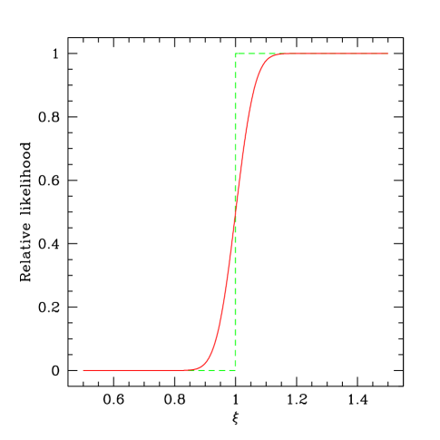
This form of the likelihood encodes the uncertainty associated with our imperfect mapping, as described by $\tau$. The effect of including the theoretical uncertainty is to smear out the drop of the likelihood function: the scale of the drop goes from $\sigma$ to $\sqrt{\sigma^{2}+\tau^{2}}$. Unfortunately, experimental bounds are usually given in the form of the lower or upper $95\%$ confidence limit only, without the possibility of deriving a form of the likelihood analogous to (14). In the absence of fuller information about the experimental value of $\sigma$, we can take in (14) the limit $\sigma\ll\tau$ and simply use the 95% CL  bound as $\xi_{\rm lim}$. This procedure leads to the likelihood function plotted in Fig. 1, showing that the inclusion of the theoretical uncertainty smears the 95% bound over the scale $\tau$. This procedure is more conservative than the usual method of simply rejecting all points below $\xi_{\rm lim}$.

We use (14) as the likelihood function for all of the upper/lower bounds listed in Table 4 along with our estimates of the corresponding theoretical uncertainty. We also discard, i.e., assign zero likelihood to all unphysical points in parameter space, i.e., those for which any of the masses becomes tachyonic or the conditions of EWSB are not satisfied. We do the same for the cases where the lightest neutralino is not the LSP.

3.2 Inputs for SM quantities

As explained in section 2, the uncertainties coming from experimental errors in the SM parameters are incorporated through four nuisance parameters: $M_{t}$, $m_{b}(m_{b})^{\overline{MS}}$, $\alpha_{\text{em}}(M_{Z})^{\overline{MS}}$ and $\alpha_{s}(M_{Z})^{\overline{MS}}$. These quantities and their uncertainties are summarized in Table 2.

Nuisance parameter	Mean value	Uncertainty	Ref.
	$\mu$	${\sigma}$ (exper.)
$M_{t}$	172.7 GeV	2.9 GeV	[24]
$m_{b}(m_{b})^{\overline{MS}}$	4.24 GeV	0.11 GeV	[25]
$\alpha_{s}(M_{Z})^{\overline{MS}}$	0.1186	0.002	[26]
$1/\alpha_{\text{em}}(M_{Z})^{\overline{MS}}$	127.958	0.048	[27]

Table 2: Experimental mean $\mu$ and standard deviation $\sigma$ for the nuisance parameters used in the analysis. For all these quantities we use a Gaussian likelihood function with the mean $\mu$ and the standard deviation $\sigma$.

Note that for the running bottom quark mass $m_{b}(m_{b})^{\overline{MS}}$ the range adopted in Table 2 is rather conservative. It arises from combining measurements from $\bar{b}b$ systems, b–flavored hadrons and high–energy processes. More recently, a much more precise determination of $m_{b}(m_{b})^{\overline{MS}}=4.19\pm 0.06\mbox{ GeV}$ has been obtained from a renormalization group improved sum rule analysis [28]. As for the fine structure constant, the dominant error comes from the hadronic contribution $\Delta\alpha_{had}=0.02758\pm 0.00035$ [27]. Note that, because of this uncertainty $\alpha_{\text{em}}(M_{Z})^{\overline{MS}}$ is not as precisely known at the scale $M_{Z}$ as at zero momentum transfer. Not included in the list of nuisance parameters are the pole mass of the $Z$ boson $M_{Z}=91.1876(21)\mbox{ GeV}$, as well as the Fermi constant $G_{F}=1.16637(1)\times 10^{-5}\mbox{ GeV}^{-2}$ [26]. As one can see, they are now known with very high precision and we fix them at their central values. Including them as nuisance parameters would not have any appreciable effect.

3.3 Derived observables

We now present the derived observables which in section 2.1 were denoted by a general symbol $\xi$. In our analysis they are computed in terms of the CMSSM parameters: $m_{0}$, $m_{1/2}$, $A_{0}$, $\tan\beta$, as well as the nuisance parameters discussed above.

In Table 3 we summarize the derived variables for which positive measurements have been made while in Table 4 we list the ones for which currently only experimental bounds exist. Lower bounds on sfermion masses have been obtained in the context of the MSSM at LEP-II and Tevatron Run II. Below we comment on some of the entries and on our procedure for their computation. Generally, to calculate Higgs and SUSY mass spectra we use the package SOFTSUSY v1.9 [29] which employs 2–loop RGEs for couplings (both gauge and Yukawa) as well as for gaugino and sfermion masses.

Derived observable	Mean value	Uncertainties		Ref.
	$\mu$	${\sigma}$ (exper.)	$\tau$ (theor.)
$M_{W}$	$80.425\mbox{ GeV}$	$34\mbox{ MeV }$	$13\mbox{ MeV }$	[27]
${\sin^{2}\theta_{\text{eff}}}$	$0.23150$	$16\times 10^{-5}$	$25\times 10^{-5}$	[27]
$\delta a_{\mu}^{\text{SUSY}}\times 10^{10}$	$25.2$	9.2	$1$	[30, 31]
$\text{BR}(\bar{B}\rightarrow X_{s}\gamma)\times 10^{4}$	$3.39$	$0.30$	$0.30$	[32]
$\Omega_{\chi}h^{2}$	0.119	0.009	$0.1\,\Omega_{\chi}h^{2}$	This work

Table 3: Summary of derived observables used in the analysis for which positive measurements have been made. As explained in the text, for each quantity we use a likelihood function with mean $\mu$ and standard deviation $s=\sqrt{\sigma^{2}+\tau^{2}}$, where $\sigma$ is the experimental uncertainty and $\tau$ our estimate of the theoretical uncertainty.

Derived observable		Constraints		Ref.
		$\xi_{\rm lim}$	$\tau$ (theor.)
$\sigma^{SI}_{p}$	UL	WIMP mass dependent	$\sim 100\%$	[33]
$\text{BR}({B}_{s}\rightarrow\mu^{+}\mu^{-})$	UL	$1.5\times 10^{-7}$	14%	[32]
$m_{h}$	LL	$114.4\mbox{ GeV}$ ($91.0\mbox{ GeV}$)	$3\mbox{ GeV}$	[22]
$\zeta_{h}^{2}$	UL	$f(m_{h})$	3%	[22]
$m_{\chi}$	LL	$50\mbox{ GeV}$	5%	[37] ([35, 36])
$m_{\chi^{\pm}_{1}}$	LL	$103.5\mbox{ GeV}$ ($92.4\mbox{ GeV}$)	5%	[34] ([35, 36])
$m_{\tilde{e}_{R}}$	LL	$100\mbox{ GeV}$ ($73\mbox{ GeV}$)	5%	[34] ([35, 36])
$m_{\tilde{\mu}_{R}}$	LL	$95\mbox{ GeV}$ ($73\mbox{ GeV}$)	5%	[34] ([35, 36])
$m_{\tilde{\tau}_{1}}$	LL	$87\mbox{ GeV}$ ($73\mbox{ GeV}$)	5%	[34] ([35, 36])
$m_{\tilde{\nu}}$	LL	$94\mbox{ GeV}$ ($43\mbox{ GeV}$)	5%	[38] ([26])
$m_{\tilde{t}_{1}}$	LL	$95\mbox{ GeV}$ ($65\mbox{ GeV}$)	5%	[34] ([35])
$m_{\tilde{b}_{1}}$	LL	$95\mbox{ GeV}$ ($59\mbox{ GeV}$)	5%	[34] ([35])
$m_{\tilde{q}}$	LL	$318\mbox{ GeV}$	5%	[39]
$m_{\tilde{g}}$	LL	$233\mbox{ GeV}$	5%	[39]

Table 4: Summary of derived observables for which only limits exist, with UL = upper limit, LL = lower limit (at $\xi_{\rm lim}$ (13), 95% CL, unless otherwise stated). The experimental limit on the spin–independent cross section for a WIMP elastic scattering on a free proton $\sigma^{SI}_{p}$ is not included in the likelihood, as explained in the text. Since the precise form of the likelihood is not available, we use the conservative procedure of including at least an estimated theoretical uncertainty $\tau$. The likelihood is then given by Eq. (14), in the limit where $\sigma\ll\tau$. The value in parenthesis indicates the more conservative bound, see the text for details. Note that theoretical errors for scalar masses are probably much larger in the focus point region, as discussed in the text.

$W$ gauge boson mass

Intrinsic theoretical uncertainties coming from higher loop effects to the $W$ boson pole mass are estimated to be $\tau(M_{W})=13\mbox{ MeV }$ [40, 41]. The parametric uncertainties are dominated by the experimental error of the top quark mass and by the hadronic contribution to the shift of the fine structure constant. Both uncertainties are fully taken into account (via $\Delta\alpha_{had}$) by marginalizing over $M_{t}$ as a nuisance parameter. We compute $M_{W}$ in the $\overline{\rm DR}$ scheme (from gauge couplings relations), including full 1–loop contributions [40].

Effective leptonic weak mixing angle

The effective leptonic weak mixing angle ${\sin^{2}\theta_{\text{eff}}}$ receives SM and SUSY contributions. In our computation we include a full 1–loop SM and full 1–loop universal $Z$–vertex supersymmetric corrections [40]. The net contribution of the non–universal corrections is negligible [42]. Intrinsic theoretical uncertainties come from higher–loop effects, which induce an uncertainty taken to be [40] $\tau({\sin^{2}\theta_{\text{eff}}})=25\times 10^{-5}$.

Note that we treat $\alpha_{\text{em}}(M_{Z})^{\overline{MS}}$ as a nuisance parameter but take $M_{W}$ and ${\sin^{2}\theta_{\text{eff}}}$ as derived quantities. This is because we use a parametrization in which the former (along with $M_{Z}$ and $G_{F}$) are taken as inputs from which one can compute the latter and compare with experiment.

The anomalous magnetic moment of the muon

The final measurement of the anomalous magnetic moment of the muon, $a_{\mu}\equiv(g-2)_{\mu}$, by the Brookhaven E821 experiment [30] $a_{\mu}^{\text{exp}}=(11659208.0\pm 5.8)\times 10^{-10}$ remains in an apparent disagreement with SM predictions. The current SM theoretical value, based on $e^{+}e^{-}$ low energy data, is [31] $a_{\mu}^{\text{SM}}=11659182.8\pm 6.3_{\text{had}}\pm 3.5_{\text{LBL}}\pm 0.3_{\text{QED+EW}})\times 10^{-10}$. The discrepancy between the two, if confirmed, could be attributed to an additional contribution from loops involving superpartners,

$$\delta a_{\mu}^{\text{SUSY}}=a_{\mu}^{\text{exp}}-a_{\mu}^{\text{SM}}=(25.2\pm 9.2)\times 10^{-10},$$ (16)

where the independent errors have been added in quadrature.

In calculating $\delta a_{\mu}^{\text{SUSY}}$ we have taken into account the full one–loop SM+SUSY contributions [43] and several two–loop corrections. The first class of two–loop corrections comprises the leading one–loop diagrams with a photon in the second loop [44]. The second class comprises diagrams with a closed loop of SM fermions or scalar fermions [45]. The last class comes from diagrams containing a closed chargino–neutralino loop [46]. As a consequence, in the CMSSM parameter space the intrinsic uncertainties are estimated to be $\tau({\delta a_{\mu}^{\text{SUSY}}})=1\times 10^{-10}$ [47]. The sign of the SUSY contribution to $a_{\mu}$ is the same as the sign of $\mu$. Since the former is positive, throughout this analysis we have assumed $\text{sign}(\mu)=+1$.

Finally, we note that, the SM value evaluated using $\tau$–data is $a_{\mu}^{\text{SM}}=(11659201.8\pm 6.3$, leading to only a $0.7\sigma$ deviation [48]. In light of this we do not feel it is justified to apply a SM prediction based on combining the two sets of data. Secondly, there appears to be potentially some discrepancy among different sets of $e^{+}e^{-}$ which again may put the claimed deviation (16) from the SM into question. Because of these outstanding problems, in subsection 4.6 we will perform a separate analysis where we exclude $a_{\mu}$ from the likelihood.

$BR(\bar{B}\rightarrow X_{s}\gamma)$

The current experimental world average value by the Heavy Flavour Averaging Group (HFAG) is [32]

$$BR({\bar{B}}\rightarrow X_{s}\gamma)_{\text{exp}}=(3.39^{+0.30}_{-0.27})\times 10^{-4},$$ (17)

which agrees rather well with the full NLO prediction of the SM [49]

$$BR({\bar{B}}\rightarrow X_{s}\gamma)_{\text{SM}}=(3.70\pm 0.30)\times 10^{-4}.$$ (18)

This clearly imposes an important constraint on any additional contributions. In the CMSSM, the assumed universality of soft mass terms leads to a particularly simple flavor structure in which no additional sources of flavor mixings beyond those due to the CKM matrix are present, the framework known as minimal flavor violation (MFV). In this case SUSY contributions arise from a loop involving the top quark and the charged Higgs boson and one of the stop–chargino exchange. In a more general flavor mixing scenario additional one–loop contributions arise due to gluino (or neutralino) and down–type squark exchange.

We compute SUSY contribution to $BR({\bar{B}}\rightarrow X_{s}\gamma)$ following the procedure outlined in Refs. [50, 51] where, in addition to full leading log corrections, large $\tan\beta$–enhanced terms arising from corrections coming from beyond the leading order (BLO) have been included. Furthermore, combined experimental constraints from $BR({\bar{B}}\rightarrow X_{s}\gamma)$ and $BR(B\rightarrow X_{s}l^{+}l^{-})$ imply that, baring highly non–standard scenarios [54], the sign of the total amplitude for the decay $\bar{B}\to X_{s}\gamma$ has to be the same as that of the SM [55].

We assume no significant additional theoretical uncertainty beyond that coming from the SM calculation. This can in part be justified by the fact that the overall SUSY contribution to $BR({\bar{B}}\rightarrow X_{s}\gamma)$ has to be small, as noted above. More importantly, we estimate that most of the uncertainties due to SUSY contributions are due to remaining uncertainties in the values of SM parameters, especially the top and bottom masses which are accounted for in their treatment as nuisance parameters. Therefore we take $\tau(BR({\bar{B}}\rightarrow X_{s}\gamma))=0.30\times 10^{-4}$.

Cosmological constraints on the dark matter density

A combination of the recent WMAP data [56] on the CMB anisotropies with other cosmological observations, such as measurements of the matter power spectrum, leads to tight constraints on the cold dark matter (CDM) relic abundance. The exact numerical value depends on a number of assumptions about the underlying cosmology (e.g., the geometry of space, the adiabaticity of initial conditions and a power–law, feature–free primordial power spectrum). It is important to keep in mind that relaxing some or all of these assumptions can considerably weaken the constraints. Furthermore, different combinations of data sets also lead to somewhat different values for the relic abundance. For definiteness, we have performed a re–analysis of CMB data from the first year of WMAP observations [56], as well as from CBI [57], VSA [58] and ACBAR [59], and combined them with the real–space power spectrum of galaxies from the SLOAN galaxy redshift survey (SDSS) [60], restricted to scales over which the fluctuations are assumed to be in the linear regime, i.e. for $k<0.1h^{-1}\,\mbox{Mpc}$, with the Hubble Space Telescope measurement [61] of the Hubble parameter $H_{0}$ ($H_{0}=100\,h\,{\mbox{k}m}/{{\rm sec}}/\mbox{Mpc}$), and with the latest supernovae observations data [62]. Assuming a flat Universe $\Lambda$CDM cosmology, the resulting constraint on the dark matter relic abundance – after marginalizing over all other relevant cosmological parameters – is well approximated by a Gaussian function with a mean and standard deviation given by

$$\Omega_{\text{CDM}}h^{2}=0.119\pm 0.009.$$ (19)

We make use of this constraint and we assume that all the CDM is made up of stable neutralinos, but we also enlarge the error to include a theoretical uncertainty in the computation of $\Omega_{\text{CDM}}h^{2}$ (see below).

A precise determination of the neutralino relic abundance $\Omega_{\chi}h^{2}$ requires an accurate treatment of the neutralino pair annihilation and coannihilation cross sections into all SM particle final states. We employ exact expressions for neutralino pair annihilation processes into all allowed final–state channels which have been computed in [63] and which are valid both near and further away from resonances and thresholds. We further include the neutralino coannihilation with the lightest chargino and next–to–lightest neutralino [64] and with the lighter stau [65] with similar precision. We include all coannihilation channels, including coannihilation with light stops [66]. We compute $\Omega_{\chi}h^{2}$ by solving the Boltzmann equation numerically as in [67].

As is well known from fixed–grid scans, in the CMSSM the values of $\Omega_{\chi}h^{2}$ typically exceeds the range given in (19), except in some rather special regions of the parameter space. Firstly, at fairly small $m_{1/2}$ and $m_{0}$, the neutralino annihilation channel into SM fermion/boson pairs via $t/u$–channel exchange of a superpartner opens up only a narrow band consistent with $\Omega_{\text{CDM}}h^{2}$ (the “bulk” region) which however is largely excluded by a lower bound on the Higgs mass and/or by a strong upper bound on allowed SUSY contribution to $BR({\bar{B}}\rightarrow X_{s}\gamma)$. Secondly, if the LSP and the next–to–LSP (NLSP) are closely degenerate in mass, then the LSP coannihilations with NLSPs near freeze–out may reduce the LSP relic density considerably. In the CMSSM, efficient coannihilation takes place along the boundary dividing neutralino and lightest stau ${\widetilde{\tau}}_{1}$ LSP regions. In addition, at large $A_{0}$ there are limited cases where the lightest stop is the NLSP and is almost degenerate in mass with the LSP [66]. Thirdly, in some cases neutralino annihilation can be enhanced via the process $\chi\chi\rightarrow f\bar{f}$ involving an $s$–channel Higgs or $Z$ boson exchange. At large $\tan\beta\sim 50$ the most significant effect comes from the CP-odd Higgs $A$ resonance (around $m_{A}\simeq 2m_{\chi}$, where $m_{\chi}$ is the lightest neutralino mass), since the $A$ couplings to down–type fermions are enhanced at large $\tan\beta$, and because, in contrast to heavy scalar Higgs exchange, the process is not $p$–wave suppressed. Finally, at very large $m_{0}$ of a few TeV the rapidly decreasing $\mu^{2}$ (from large positive to negative values) causes the higgsino component of the LSP to increase which, in a narrow focus point (FP) region (of still positive $\mu^{2}$) allows $\Omega_{\chi}h^{2}$ to pass through the favored range (19), before becoming too small.

The theoretical uncertainty involved in computing $\Omega_{\chi}h^{2}$ varies greatly depending on the case. Errors come from computing the Higgs and superpartner mass spectrum at finite (two–loop) order in RGEs, a scale dependence, finite numerical accuracy in solving the Boltzmann equation, some residual uncertainties in computing the gauge couplings, as well as potentially much larger errors in computing top and bottom Yukawa couplings and Higgs widths. The choice of the scale at which one minimizes the effective potential has a minor effect [17]. A numerical algorithm of solving the Boltzmann equation is very accurate and in the bulk region has an estimated error of a few per cent [68, 63], which is comparable with the observational error in (19).

In the bulk region where $\Omega_{\chi}h^{2}$ primarily depends on the $t/u$–channel exchange of sleptons, uncertainties in the calculation of the SUSY spectrum are $\mathcal{O}(1\%)$ (for moderate values of the CMSSM mass parameters, even at large $\tan\beta$) and therefore under control [69]. On the other hand, the accuracy is much poorer in the regions of special cosmological interest that have been mentioned above. In the coannihilation regions $\Omega_{\chi}h^{2}$ is sensitive to $e^{-\Delta m/T}$, where $\Delta m=m_{\rm NLSP}-m_{\chi}$ is the difference between the mass of the NLSP $m_{\rm NLSP}$ and $m_{\chi}$. Even a small variation of $\mathcal{O}(1\%)$ in $\Delta m$ can lead to $\sim 30\%$ variations in $\Omega_{\chi}h^{2}$ [71]. This sort of error is inherent in current determinations of the mass of ${\widetilde{\tau}}_{1}$ which is the NLSP in large parts of the $(m_{1/2},m_{0})$ plane. Larger uncertainties arise if the NLSP is the ${\widetilde{t}}_{1}$ since the shift in its mass $10\%$ can lead to order–of–magnitude discrepancies in the prediction of the relic density [69]. In the CP–odd Higgs resonance region one finds a strong suppression of $\Omega_{\chi}h^{2}$ for broad ranges of $m_{1/2}$ and $m_{0}$. In the CMSSM this occurs for large $\tan\beta$ where effects of the bottom Yukawa coupling $h_{b}$ on the RGE running are important and reduce $m_{A}$ compared to the low $\tan\beta$ regime. The relic density is further suppressed by the enhancement of the coupling $Ab\bar{b}$ which is proportional to $h_{b}$. Special attention must also be paid to the computation of the Higgs boson width which receives sizable radiative corrections. We include one–loop QCD corrections [70] as well as those due to (QCD corrected) Yukawa vertices. Still, unknown two–loop corrections to $h_{b}$ may cause an uncertainty of up to $30\%$ [71]. In the FP region, a determination of $\mu$ is strongly sensitive to two–loop corrections proportional to $h_{t}$, whose computation requires special care, and can lead to $\sim 100\%$ errors in the computation of $\Omega_{\chi}h^{2}$ [71].

In addition to the theoretical errors discussed above, the value of $\Omega_{\chi}h^{2}$ depends on the top and bottom masses, as well as $\alpha_{\text{em}}(M_{Z})^{\overline{MS}}$. In particular, we have found that the seemingly small experimental error in $\alpha_{\text{em}}(M_{Z})^{\overline{MS}}$ leads, indirectly, via its effect on the SM gauge couplings $g_{1,2}$, to a variation in $\Omega_{\chi}h^{2}$ of order $10\%$. All of these effects are accounted for by our use of the nuisance parameters.

The error in the quantity $\Omega_{\chi}h^{2}$ can thus be very sensitive to which (co)annihilation process is most efficient. This makes it difficult to evaluate the theoretical uncertainty in $\Omega_{\chi}h^{2}$. Given the above discussion we estimate $\tau(\Omega_{\chi}h^{2})=10\%$ in the bulk of the parameter space although we are aware that in the FP region the error is almost certainly much larger. We add this error in quadrature to the observational error $\sigma(\Omega_{\text{CDM}}h^{2})=0.009$ in (19) and obtain the Gaussian with the following mean and standard deviation,

$$\Omega_{\chi}h^{2} = 0.119\pm\sqrt{(0.009)^{2}+(0.1\,\Omega_{\chi}h^{2})^{2}}$$ (20)

$$= 0.119\pm 0.009\,\sqrt{1+1.75\,(\Omega_{\chi}h^{2}/0.119)^{2}}.$$ (21)

Note that the theoretical uncertainty is of the same order as the uncertainty from current cosmological determinations of $\Omega_{\text{CDM}}h^{2}$.

We now comment on some of the derived variables for which the $95\%$ CL experimental upper/lower limits have been presented in Table 4. We start, however, with the only observable which is not included in the likelihood.

Direct detection of dark matter

Assuming the Galactic DM halo is mostly made up of neutralinos, it may be possible to directly detect them via their elastic scatterings off nuclei, or indirectly via their annihilation products. Direct DM detection in SUSY frameworks has been investigated by many authors [72]. The CDMS Collaboration (CDMS–II) has recently improved their previous upper limit on the spin–independent dark matter WIMP elastic scattering cross section on a free proton, $\sigma^{SI}_{p}$, down to some $2\times 10^{-7}\,\mbox{pb}$ (at low WIMP mass) [73]. Comparable upper limits have also been set up by the Edelweiss–I [74] and ZEPLIN–I [75] experiments.

However, several questions regarding the properties of the DM halo (e.g., the existence of clumps of DM and the value of the local halo mass density) remain unsettled. Recent numerical N–body simulations of large structure formation have revealed a large number of overdense regions surviving until today [76]. It is possible that an improved sensitivity of the simulations will reveal further, and finer, clumpiness. The clumps may contain a sizable fraction of the total dark matter halo, of the order of 10%. It is therefore not unlikely that locally (at the Earth’s location) the DM density may be significantly different from the usually assumed average value of $\rho_{\chi}=0.3\mbox{ GeV}/{\mbox{cm}}^{3}$.

It is worth remembering that, in translating null experimental results for an elastic WIMP–target cross section into upper limits on $\sigma^{SI}_{p}$, not only the local DM density enters but also a WIMP velocity distribution. This is usually taken to be Maxwellian with a peak at $220~{}{\mbox{k}m}/{\rm sec}$ with an estimated error of between 20 and $50~{}{\mbox{k}m}/{\rm sec}$. While this leads to an additional uncertainty in $\sigma^{SI}_{p}$, it is actually tiny compared with the uncertainty of the actual WIMP density at the position of the Earth caused by cuspiness. In view of the above discussion, in our opinion upper experimental limits on $\sigma^{SI}_{p}$ should not be used to constrain supersymmetric parameters with the same degree of reliability as from collider searches.

In computing $\sigma^{SI}_{p}$ in the CMSSM, we include full supersymmetric contributions which have been derived by several groups [77, 78, 79, 80, 81]. $\sigma^{SI}_{p}$ can be expressed as

$$\sigma^{SI}_{p}=\frac{4}{\pi}\mu^{2}_{p}f_{p}^{2}$$ (22)

where $\mu_{p}=m_{p}m_{\chi}/(m_{p}+m_{\chi})$ is the reduced mass of the WIMP–proton system. (For spin–independent interactions of neutralinos, and more generally Majorana WIMPs, there is no need to consider an analogous quantity on a free neutron since $\sigma^{SI}_{n}=\sigma^{SI}_{p}$.)

The coefficients $f_{p,n}$ can be expressed as [77]

$${f_{p}\over m_{p}}=\sum_{q=u,d,s}{f_{Tq}^{(p)}\over m_{q}}f_{q}~{}+~{}{2\over 27}f^{(p)}_{TG}\sum_{q=c,b,t}{f_{q}\over m_{q}}+...$$

where $f^{(p)}_{TG}=1-\sum_{q=u,d,s}f^{(p)}_{Tq}$, and nuclear form factors $f_{Tq}^{(p)}$ are defined via $\langle p|m_{q}\bar{q}q|p\rangle=m_{p}f_{Tq}^{(p)}$ ($q=u,d,s$), and analogously for the neutron. The masses and ratios $B_{q}=\langle p|{\bar{q}}q|p\rangle$ of light constituent quarks in a nucleon come with some uncertainties. For definiteness, we adopt the set of input parameter given in [80] and assume $m_{u}/m_{d}=0.553\pm 0.043$, $m_{s}/m_{d}=18.9\pm 0.8$, and $B_{d}/B_{u}=0.73\pm 0.02$, as well as

$$f^{(p)}_{Tu}=0.020\pm 0.004,\quad f^{(p)}_{Td}=0.026\pm 0.005,\quad f^{(p)}_{Ts}=0.118\pm 0.062,$$ (23)

$$f^{(n)}_{Tu}=0.014\pm 0.003,\quad f^{(n)}_{Td}=0.036\pm 0.008,\quad f^{(n)}_{Ts}=0.118\pm 0.062,$$ (24)

and for the parton density functions we employ the CTEQ6L set [82] evaluated at the QCD scale defined by the averaged squark mass and neutralino mass $Q\approx\sqrt{M^{2}_{\tilde{q}}-m_{\chi}^{2}}$. The nuclear form factors $f_{Ts}^{(p,n)}$ come with a large error and these are the ones that provide the dominant contribution to $\sigma^{SI}_{p}$. This has a rather significant impact on the size of $\sigma^{SI}_{p}$ [83], unless $\tan\beta$ is very small.

$BR(B_{s}\rightarrow\mu^{+}\mu^{-})$

The latest $95\%$ CL experimental upper limits from the DØ Run II and CDF Run II experiments at Fermilab are, respectively,

$$BR(B_{s}\rightarrow\mu^{+}\mu^{-}) < 2.0\times 10^{-7}\ \ \ {\rm(CDF)~{}\cite[cite]{[\@@bibref{}{cdfbsmm05}{}{}]}},$$ (25)

$$BR(B_{s}\rightarrow\mu^{+}\mu^{-}) < 3.7\times 10^{-7}\ \ \ {\rm(D\O)~{}\cite[cite]{[\@@bibref{}{dzerobsmm05prelim}{}{}]}}.$$ (26)

A combined $95\%$ CL limit is $BR(B_{s}\rightarrow\mu^{+}\mu^{-})<1.5\times 10^{-7}$ [87]. Ultimately, assuming the integrated luminosity of $8\,\mbox{fb}^{-1}$, a combined CDF and DØ limit is expected to reach some $2\times 10^{-8}$ [88] which is significantly above the SM prediction [89]

$$BR(B_{s}\rightarrow\mu^{+}\mu^{-})_{\mathrm{SM}}=\left(3.42\pm 0.54\right)\times 10^{-9}.$$ (27)

We compute the SUSY contribution to $BR(B_{s}\rightarrow\mu^{+}\mu^{-})$ by following a full one–loop calculation of Ref. [90] which assumes MFV. Furthermore we include $\tan\beta$ enhanced corrections to the bottom quark mass [91]. The parametric uncertainties are associated with an error in the decay constant $f_{B_{s}}$, which arises from lattice calculations, and an error in the bottom quark mass [92]. The latter is accounted for by the MC procedure, while the former is of order $10\%$. Unknown higher order corrections are of order $10\%$ [93]. Therefore we use a total theoretical error of 14%, obtained by adding the above uncertainties in quadrature.

The lightest MSSM Higgs boson mass

A final LEP–II lower bound on the SM Higgs mass is $m_{H_{\text{SM}}}>114.4\mbox{ GeV}$ (95 % CL) [22]. The bound applies to the lightest Higgs boson $h$ in the MSSM if its coupling to the $Z$ boson is SM–like, i.e. if $\zeta_{h}^{2}\equiv g^{2}_{ZZh}/g^{2}_{ZZH_{\text{SM}}}=\sin^{2}(\beta-\alpha)\simeq 1$. This occurs in the decoupling regime where $m_{A}\gg m_{Z}$. For arbitrary values of $m_{A}$, the LEP–II Collaboration has set 95% CL bounds on $m_{h}$ and $m_{A}$ as a function of $\zeta_{h}^{2}$ [22], with the lower bound of $m_{h}>91\mbox{ GeV}$ for $m_{h}\sim m_{A}$ and $\zeta_{h}^{2}\ll 1$ [22]. In this low–mass region we use a cubic spline to interpolate between some selected points in $m_{h}$ and derive the corresponding 95% CL bound, which is then smeared with a theoretical uncertainty $\tau$ of 3%. The intrinsic theoretical error in computing $m_{h}$, after taking into account effects of the renormalization scale dependence, in the CMSSM has been estimated to be $\tau(m_{h})=3\mbox{ GeV}$ [94, 95]. The parametric uncertainty coming from the errors in top quark mass and the strong coupling constant are accounted for by taking them as nuisance parameters.

As mentioned above, we compute the lightest Higgs mass following the SOFTSUSY v1.9 package [29], where full one–loop and leading two–loop corrections and two–loop effects on the EWSB conditions are included.

Superpartner masses

Below we comment on some limits on superpartner masses. Since currently there is no information available on the likelihood function for sparticle masses, we make use of the experimental error of 95% CL and of the likelihood given in Eq. (14).

The parametric uncertainties in the sparticle masses coming from the SM variables are accounted for via the nuisance parameters. The authors of Ref. [69] have argued that the theoretical uncertainties in the computation of SUSY masses are of order $\mathcal{O}(1\%)$ except in some special regions of the parameter space (such as the FP region) which require a separate treatment. Conservatively we take $\tau=5\%$ for each computed superpartner mass and use it to smear out the 95% CL experimental lower limit on its mass, as explained in section 3.1.

Neutralino LSP mass

In the context of the CMSSM, LEP–II provides an absolute lower bound on the mass of the lightest neutralino LSP $\chi_{1}$ (in this work denoted simply by $\chi$) [37]

$$m_{\chi}>50\mbox{ GeV}.$$ (28)

Chargino mass

Chargino mass has been excluded up to $m_{\chi_{1}^{\pm}}>103.5\mbox{ GeV}$ [34], provided that $m_{\tilde{\nu}}>300\mbox{ GeV}$, where $m_{\tilde{\nu}}$ stands for the lightest sneutrino mass which in the CMSSM is ${\tilde{\nu}}_{\tau}$. However, when the mass difference $m_{\chi_{1}^{\pm}}-m_{\chi}\lesssim 3\mbox{ GeV}$, as in the FP region, then the bound is relaxed to $m_{\chi^{\pm}_{1}}>92.4\mbox{ GeV}$ [34]. The latter bound is also applied when $m_{\tilde{\nu}}<300\mbox{ GeV}$.

Slepton masses

Combined slepton mass limits have been obtained by the LEP SUSY working group [34]. The overall limits are

$$m_{\tilde{e}_{R}}>100\mbox{ GeV},\qquad m_{\tilde{\mu}_{R}}>95\mbox{ GeV},\qquad m_{\tilde{\tau}_{1}}>87\mbox{ GeV}.$$ (29)

These limits are valid provided that $m_{\tilde{l}}-m_{\chi}>10\mbox{ GeV}$. Otherwise we apply the more conservative bound $m_{\tilde{l}_{R}}>73\mbox{ GeV}$ [35, 36].

For the sneutrino, in the context of the CMSSM, the DELPHI collaboration has obtained the following limit [38]

$$m_{\tilde{\nu}}>94\mbox{ GeV},$$ (30)

provided $m_{\tilde{\nu}}-m_{\chi}>10\mbox{ GeV}$. Otherwise we apply $m_{\tilde{\nu}}>43\mbox{ GeV}$ [26].

Squark masses

Combined limits on the lightest stop and sbottom masses from LEP–II are [34]

$$m_{\tilde{t}_{1},\tilde{b}_{1}}>95\mbox{ GeV},$$ (31)

provided $m_{\tilde{t}_{1},\tilde{b}_{1}}-m_{\chi}>10\mbox{ GeV}$. Otherwise we apply the more conservative limits obtained by the ALEPH Collaboration [35]

$$m_{\tilde{t}_{1}}>65\mbox{ GeV}\quad\text{and}\quad m_{\tilde{b}_{1}}>59\mbox{ GeV}.$$ (32)

Finally, for the two first generations, the DØ Run II Collaboration obtained [39]

$$m_{\tilde{q}}>318\mbox{ GeV}.$$ (33)

4 Results

We now present the results of our study in terms of high relative posterior probability regions for CMSSM parameters and superpartner masses (section 4.1) and the implications for other observables (section 4.2). In section 4.3 we compare those results with the mean quality of fit statistics, while in section 4.4 the prospects for direct detection of DM are presented. Correlations among observables are depicted in section 4.5, while section 4.6 is concerned with the influence that the measurement of the anomalous magnetic moment has on our conclusions.

Our statistical inferences are drawn from multiple MC chains, which contain a total of about $3\times 10^{5}$ to $4\times 10^{5}$ samples. For more details about our numerical implementation of the MCMC algorithm, see appendix A.

4.1 High probability regions for parameters and superpartners masses

Figure 2: The 2–dimensional probability densities in the planes spanned by the CMSSM parameters: $m_{1/2}$, $m_{0}$, $A_{0}$ and $\tan\beta$ for the “4 TeV range” analysis (see Table 1). The pdf’s are normalized to unity at their peak. The inner (outer) blue solid contours delimit regions encompassing 68% and 95% of the total probability, respectively. All other parameters in each plane have been marginalized over.

Figure 3: The 2–dimensional relative probability densities as in Fig. 2 but for the “2 TeV range” analysis and for the planes $(m_{1/2},m_{0})$ and $(\tan\beta,m_{0})$ only. Imposing a prior range $m_{0}<2\mbox{ TeV}$ modifies substantially the inferences about the high probability regions for $m_{0}$.

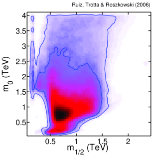
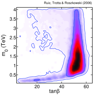
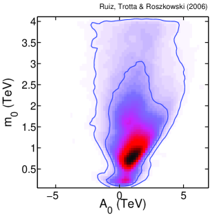
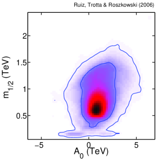
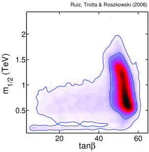
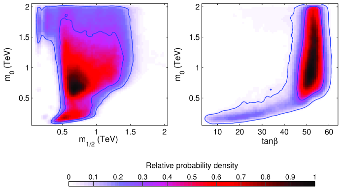
In the six panels of Fig. 2, we show the 2–dimensional posterior relative probability density functions $p(\theta_{i},\theta_{j}|d)$, where $(\theta_{i},\theta_{j})=(m_{1/2},m_{0})$, $(\tan\beta,m_{0})$, $(A_{0},m_{0})$, $(A_{0},m_{1/2})$, $(\tan\beta,m_{1/2})$ and $(\tan\beta,A_{0})$, for the “4 TeV range” case which we will treat as our default choice. In each panel all other basis parameters have been marginalized over. Redder (darker) regions correspond to higher probability density. Inner and outer blue (dark) solid contours delimit regions of 68% and 95% of the total probability, respectively. In all the 2–dimensional plots, the MC samples have been divided into $70\times 70$ bins. Jagged contours are a result of a finite resolution of the MC chains.

It is clear that the structure of the parameter space is rather complex. In particular, in the left top and bottom panels at $m_{1/2}\simeq 0.2\mbox{ TeV}$ we can see a narrow high–probability funnel induced by the light Higgs boson resonance, which was also observed in the analysis of Ref. [17]. The presence of such narrow wedges makes the exploration challenging for the MCMC procedure, and much harder for a fixed–grid scan.

Values of $m_{0}\mathrel{\hbox to0.0pt{\lower 4.0pt\hbox{\hskip 1.0pt$\sim$}\hss}\raise 1.0pt\hbox{$<$}}2\mbox{ TeV}$ are favored, but larger values are definitely not excluded. In particular, the 95% probability region extends up to the upper prior range for $m_{0}$, a clear sign that the data is not powerful enough to constrain this parameter sufficiently (we comment further on this issue below). The most probable region in the $(m_{1/2},m_{0})$ plane is centered around the point

$$m_{1/2}\simeq 0.7\mbox{ TeV},\qquad m_{0}\simeq 0.8\mbox{ TeV}.$$ (34)

The region encompassing $68\%$ of joint probability is roughly bounded by $0.5\mbox{ TeV}\mathrel{\hbox to0.0pt{\lower 4.0pt\hbox{\hskip 1.0pt$\sim$}\hss}\raise 1.0pt\hbox{$<$}}m_{1/2}\mathrel{\hbox to0.0pt{\lower 4.0pt\hbox{\hskip 1.0pt$\sim$}\hss}\raise 1.0pt\hbox{$<$}}1.5\mbox{ TeV}$, because of the efficiency of both the stau coannihilation and/or the pseudoscalar resonance. A sharp probability drop above $m_{1/2}\mathrel{\hbox to0.0pt{\lower 4.0pt\hbox{\hskip 1.0pt$\sim$}\hss}\raise 1.0pt\hbox{$>$}}1.5\mbox{ TeV}$, almost independent of $m_{0}$, is caused by a combination of the relic abundance and the $\delta a_{\mu}^{\text{SUSY}}$ constraints. At smaller $m_{0}$ the boundary bends because below it the neutralino is not the LSP. Large values of $\tan\beta$ between about 45 and 55 are definitely more favored but smaller values are also allowed, in particular for small $m_{0}\mathrel{\hbox to0.0pt{\lower 4.0pt\hbox{\hskip 1.0pt$\sim$}\hss}\raise 1.0pt\hbox{$<$}}0.5\mbox{ TeV}$ (upper right panel), as a consequence of the light Higgs boson resonance.

The large $m_{0}$ region, starting from the upper part of the $68\%$ probability contour, corresponds to a wide range of possible positions of the FP region. For each fixed choice of parameters, the FP region consistent with the CDM abundance is actually very narrow, but its position varies widely along $m_{0}$ when we marginalize over all the other parameters.

We observe that $A_{0}$ is largely uncorrelated with other variables, and its pdf presents a strong peak around $A_{0}\simeq 0.8\mbox{ TeV}$. The high probability contours for $A_{0}$ are well within the prior range ($|A_{0}|<7\mbox{ TeV}$), which indicates that this constraint is robust with respect to changes to the prior.

In order to examine the sensitivity of these results to the assumed ranges of CMSSM parameters, i.e., the prior used, in Fig. 3 we plot the 2–dimensional pdf’s $p({m_{1/2}},{m_{0}}|d)$ and $p({\tan\beta},{m_{0}}|d)$ for the “2 TeV range”. This is similar to the prior used by the authors of Ref. [17], and for this case we find a fairly good general agreement with their results. However, several differences in the treatment of uncertainties, in the data employed and in the accuracy of the theoretical predictions add up to appreciable differences in the details of the results.

It is important to stress that by imposing an upper prior range $m_{0}<2\mbox{ TeV}$ one cuts away a large region of parameter space which is not excluded by the data (the FP region at large $m_{0}$, compare with the corresponding panels in Fig. 2). Therefore, inferences on high probability regions for large $m_{0}$ are different for the “2 TeV range” and the “4 TeV range” cases. This means that current data is not informative enough to strongly constrain the value of $m_{0}$ independently of prior information, i.e. the prior range one chooses to use. The main reason behind this is the presence of the FP region which so far has not been investigated by MCMC techniques. On the other hand, results for the other CMSSM parameters $m_{1/2},\tan\beta$ and $A_{0}$ do not vary appreciably if one changes the prior ranges, as we now discuss.

Figure 4: The 1–dimensional relative probability densities $p({\theta_{i}}|d)$ for each of the CMSSM parameter, $\theta_{i}=m_{0}$, $m_{1/2}$, $A_{0}$ and $\tan\beta$. All other parameters have been marginalized over. The two curves compare the results for two different prior ranges (see Table 1).

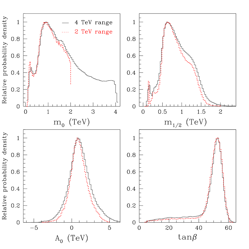
In Fig. 4 we show the posterior 1–dimensional pdf $p({\theta_{i}}|d)$ for each of the CMSSM parameters, with all the other basis parameters marginalized over. The 1–dimensional pdf’s contain the complete statistical information about each of the CMSSM variables, fully accounting for all sources of uncertainty included in the analysis. We plot results for both the “2 TeV range” and the “4 TeV range” to facilitate the comparison between the two. In the upper left panel, we note that the pdf’s for $m_{0}\leq 2\mbox{ TeV}$ are in excellent agreement for both ranges, but above that value the posterior pdf for the “2 TeV range” is sharply cut by the prior. On the contrary, the pdf for the “4 TeV range” extends all the way to $4\mbox{ TeV}$. Since the posterior does not drop to zero before reaching the prior range of $4\mbox{ TeV}$, it is likely that by allowing even larger values of $m_{0}$ one would find non–negligible probability densities even there. This is caused by a high sensitivity of the position of the FP region along the $m_{0}$ axis to the Yukawa couplings $h_{t}$ and $h_{b}$. The effect is partially accommodated by treating the top and bottom masses in the nuisance parameters. However, as explained in the discussion following Eq. (19), the computation of $\mu$ and as a result of $\Omega_{\chi}h^{2}$ is highly uncertain in the FP region. At present this makes it difficult to make a more definitive statement about the region $m_{0}\mathrel{\hbox to0.0pt{\lower 4.0pt\hbox{\hskip 1.0pt$\sim$}\hss}\raise 1.0pt\hbox{$>$}}2\mbox{ TeV}$ other than that present data does not strongly constrain it. In fact, the upper $95\%$ probability region for the “4 TeV range” extends to $m_{0}<3.66\mbox{ TeV}$. For smaller $m_{0}$, the bulk of the pdf lies around $0.5\mbox{ TeV}\mathrel{\hbox to0.0pt{\lower 4.0pt\hbox{\hskip 1.0pt$\sim$}\hss}\raise 1.0pt\hbox{$<$}}m_{0}\mathrel{\hbox to0.0pt{\lower 4.0pt\hbox{\hskip 1.0pt$\sim$}\hss}\raise 1.0pt\hbox{$<$}}1.5\mbox{ TeV}$.

Constraints on the other CMSSM parameters are largely independent of the adopted prior ranges. The bulk of the pdf for $m_{1/2}$ lies around $m_{1/2}\approx 0.75\mbox{ TeV}$, with the 68% region within $0.52\mbox{ TeV}<m_{1/2}<1.26\mbox{ TeV}$, with again a narrow peak due to the light Higgs resonance at smaller values. For the “4 TeV range” this narrow peak is more pronounced, because in this case one integrates over a larger range for $m_{0}$, compare with the upper left panel of Fig. 2. In the lower left panel of Fig. 4, the peak around $A_{0}\simeq 0.8\mbox{ TeV}$ is again clearly visible and almost independent of the prior used. We notice that the 68% region is bounded by $-0.34\mbox{ TeV}<A_{0}<2.41\mbox{ TeV}$ and thus $A_{0}=0$ lies close to its boundary. This is an interesting result (which can also be seen in Ref. [17]) in light of the fact that most of fixed–grid scans (with a few exceptions [21, 96]) have assumed $A_{0}=0$. Finally, in the last panel, the 1–dimensional pdf for $\tan\beta$ shows a preference for large values, with the $68\%$ region given by $38.5<\tan\beta<54.6$. Regions containing 68% and 95% of posterior probability for the CMSSM parameters are summarized in Table 5.

	“2 TeV  range”		“4 TeV  range”
Parameter	68% region	95% region	68% region	95% region
$m_{0}$ (TeV)	$<1.36$	$<1.88$	$<2.10$	$<3.66\mbox{ TeV}$
$m_{1/2}$ (TeV)	$(0.54,1.20)$	$(0.26,1.48)$	$(0.52,1.26)$	$(0.20,1.61)$
$A_{0}$ (TeV)	$(-0.18,2.01)$	$(-1.44,3.40)$	$(-0.34,2.41)$	$(-1.95,4.31)$
$\tan\beta$	$(44.1,54.9)$	$(16.0,58.0)$	$(38.5,54.6)$	$(13.6,57.8)$

Table 5: CMSSM parameter ranges corresponding to 68% and 95% of posterior probability (all other parameters marginalized over) for the two different prior choices, the “2 TeV  range” and the “4 TeV range”.

Super–	“2 TeV  range”		“4 TeV  range”
partner	68%	95%	68%	95%
$\chi_{1}^{0}$	$(0.22,0.52)$	$(0.10,0.64)$	$(0.22,0.55)$	$(0.07,0.70)$
$\chi_{1}^{\pm}$	$(0.42,0.98)$	$(0.16,1.20)$	$(0.36,1.00)$	$(0.11,1.25)$
$\widetilde{g}$	$(1.27,2.64)$	$(0.70,3.19)$	$(1.25,2.80)$	$(0.54,3.51)$
$\tilde{e}_{R}$	$(0.66,1.69)$	$(0.30,1.97)$	$(0.80,2.93)$	$(0.33,3.85)$
$\tilde{\nu}$	$(0.68,1.49)$	$(0.42,1.76)$	$(0.79,2.63)$	$(0.46,3.57)$
$\tilde{\tau}_{1}$	$(0.36,1.03)$	$(0.23,1.41)$	$(0.42,2.12)$	$(0.25,3.31)$
$\tilde{q}_{R}$	$(1.47,2.61)$	$(1.10,3.11)$	$(1.60,3.50)$	$(1.18,4.49)$
$\tilde{t}_{1}$	$(1.09,2.04)$	$(0.82,2.48)$	$(1.17,2.44)$	$(0.87,3.22)$
$\tilde{b}_{1}$	$(1.23,2.26)$	$(0.98,2.74)$	$(1.33,2.79)$	$(1.03,3.66)$

Table 6: Selected superpartner mass ranges (in TeV) containing 68% and 95% of posterior probability (all other parameters marginalized) for the two different prior choices, the “2 TeV range” and the “4 TeV range”.

Figure 5: As in Fig. 4, but for the masses of several representative superpartners.

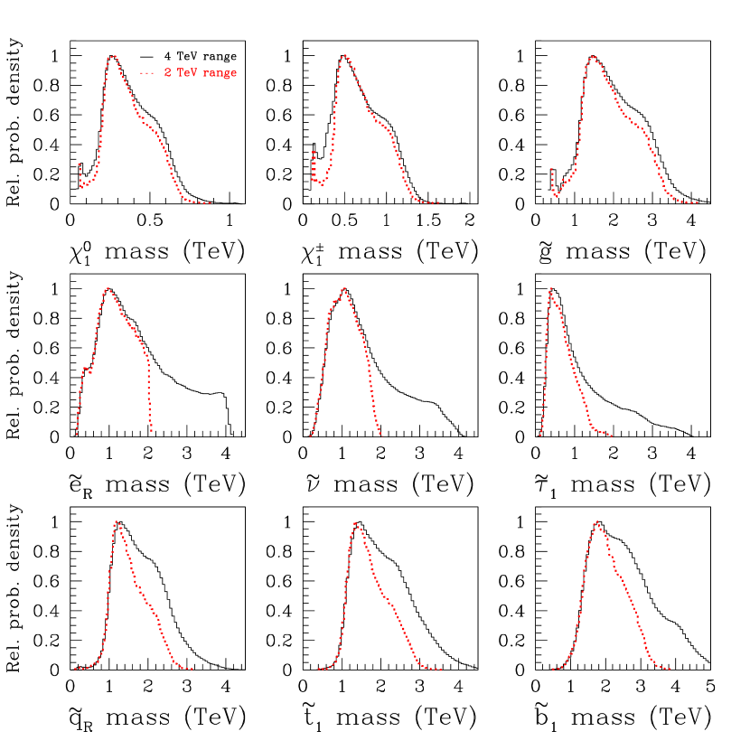
In Fig. 5 we show 1–dimensional pdf’s for several superpartners masses, and the corresponding 68% and 95% probability regions are given in Table 6. Note that the 95% CL experimental bounds on the superpartner masses have been included in the likelihood (and smeared out by corresponding theoretical uncertainties), as explained in section 3.1. The masses of the gluino $\widetilde{g}$, the lightest chargino $\chi_{1}^{\pm}$ and the LSP neutralino $\chi$, which are proportional mainly to $m_{1/2}$, are basically the same for both prior ranges, in agreement with the result for $m_{1/2}$ displayed in Fig. 4. In contrast, the pdf’s for the masses of the sfermions exhibit a sharp cutoff in the “2 TeV range” case, as a consequence of a basic mass relation $m^{2}_{{\tilde{f}}_{L,R}}\simeq m_{0}^{2}+c_{{\tilde{f}}_{L,R}}m_{1/2}^{2}$. Therefore the prior cut on $m_{0}$ for “2 TeV range” impacts on the posterior probability distribution for the sfermions as well. Nevertheless, for the squarks the relative probability peaks below some $2\mbox{ TeV}$ which is generally well within the LHC reach. As a result, the integrated probability for $m_{\tilde{q}_{R}}<2.5\mbox{ TeV}$ is 85%. For comparison, we find $m_{\widetilde{g}}<2.7\mbox{ TeV}$ with 78% probability and $m_{\chi_{1}^{\pm}}<0.8\mbox{ TeV}$ with 65% probability. We will come come back to the issue of the posterior probability distribution for the superpartners in subsection 4.6.

4.2 High probability regions for other observables

Figure 6: The 2–dim relative probability density $p({\Omega_{\chi}h^{2}},{\theta_{i}}|d)$, where $\theta_{i}=m_{0}$, $m_{1/2}$ and $\tan\beta$. Note that the measured value of $\Omega_{\chi}h^{2}$, Eq. (19), has been included in computing the relative probability density.

Figure 7: As in Fig. 6, but for $\delta a_{\mu}^{\text{SUSY}}$. The measured value of $\delta a_{\mu}^{\text{SUSY}}$, Eq. (16), has been included.

Figure 8: As in Fig. 6, but for $BR({\bar{B}}\rightarrow X_{s}\gamma)$. The measured value of $BR({\bar{B}}\rightarrow X_{s}\gamma)$, Eq. (17), has been included.

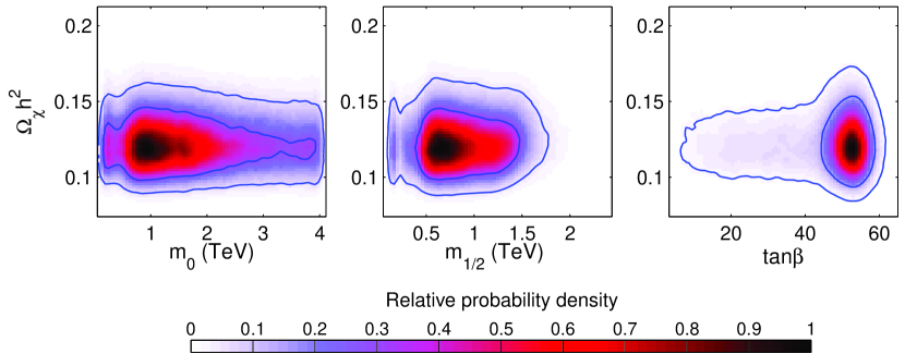
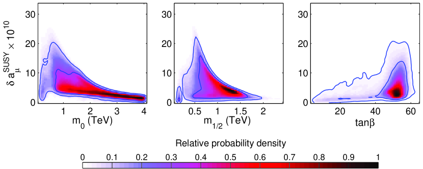
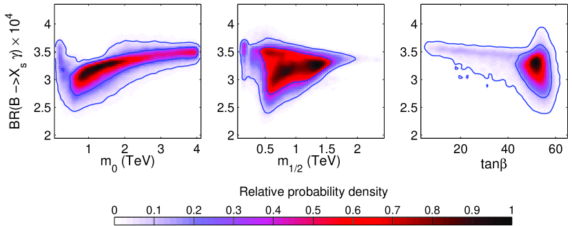
Our MCMC approach allows us to investigate the joint posterior probability distribution between CMSSM parameters and the various observables, as explained in section 2.1. In Figs. 6 – 9 we plot the joint pdf for $\Omega_{\chi}h^{2}$, $\delta a_{\mu}^{\text{SUSY}}$, $BR({\bar{B}}\rightarrow X_{s}\gamma)$, $BR(B_{s}\rightarrow\mu^{+}\mu^{-})$, respectively, and $m_{0}$, $m_{1/2}$ and $\tan\beta$ (all other parameters in each panel are marginalized over). All plots correspond to the “4 TeV range”. (See also column one in Table 9.) We stress that the joint pdf is obtained by taking into account observational constraints from all the derived variables, including the one plotted along the vertical axis.

In Fig. 6, the pdf peaks around $m_{0}\approx 1\mbox{ TeV}$ and $\Omega_{\chi}h^{2}\approx 0.12$, with all values of $m_{0}$ up to $4\mbox{ TeV}$ compatible with the observed cosmological DM abundance. This is another demonstration that the narrow “WMAP strips” – which appear when including only two parameters of the CMSSM at a time (see, e.g., [97, 15]) – actually widen considerably to cover a large region of parameter space when all the variables are taken simultaneously into account. Not surprisingly therefore, we do not find a strong correlation between $\Omega_{\chi}h^{2}$ and the CMSSM parameters.

In the planes spanned by $\delta a_{\mu}^{\text{SUSY}}$ and the CMSSM parameters (Fig. 7), we observe a strong anti–correlation between $\delta a_{\mu}^{\text{SUSY}}$ and both $m_{0}$ and $m_{1/2}$. This is a simply a reflection of the decreasing CMSSM contributions to $\delta a_{\mu}^{\text{SUSY}}$ with increasing superpartner masses. In general, the posterior distribution for $\delta a_{\mu}^{\text{SUSY}}$ is quite skewed with respect to the likelihood, which represents the experimental measurement. The posterior pdf tends to prefer values of $\delta a_{\mu}^{\text{SUSY}}$ close to zero. We comment further on this below.

For $BR(\bar{B}\rightarrow X_{s}\gamma)$, Fig. 8 shows a positive correlation with the masses, with the SM value being reached in the asymptotic regime of large $m_{1/2}$ and $m_{0}$. We also see that the peak in the pdf is centered slightly below the experimental central value given in Eq. (17).

Figure 9: As in Fig. 6, but for $BR(B_{s}\rightarrow\mu^{+}\mu^{-})$. The upper limit of $BR(B_{s}\rightarrow\mu^{+}\mu^{-})<1.5\times 10^{-7}$ has been included.

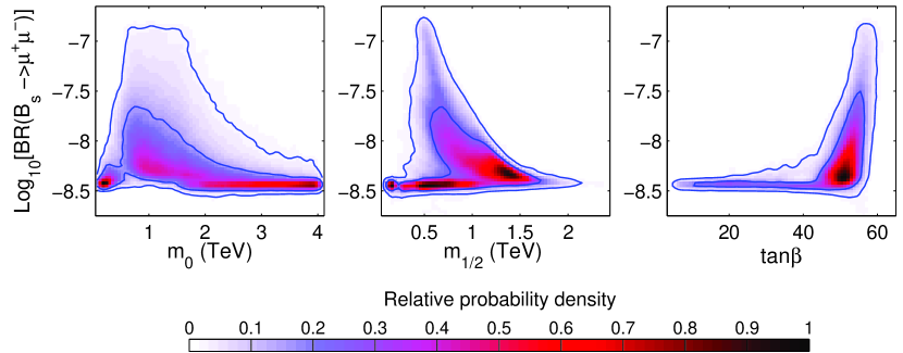
In Fig. 9 we show the 2–dimensional pdf for $BR(B_{s}\rightarrow\mu^{+}\mu^{-})$ and $m_{1/2}$, $m_{0}$ and $\tan\beta$. As expected, the SUSY contribution decreases with increasing superpartner masses and rapidly increases proportionally to $\tan^{6}\beta$. Most of the high relative probability density lies close to the SM prediction given in of Eq. (27) [89]. The 1–dimensional (2 tails) regions encompassing 68% and 95% of probability are

$$3.5\times 10^{-9}<BR(B_{s}\rightarrow\mu^{+}\mu^{-})<1.68\times 10^{-8} (68\%\text{ region}),$$ (35)

$$3.3\times 10^{-9}<BR(B_{s}\rightarrow\mu^{+}\mu^{-})<7.50\times 10^{-8} (95\%\text{ region}).$$

The current CDF and DØ limits are thus only approaching the 95% probability region. The 68% (95%) region extends just below (well above) the Tevatron reach of about $2\times 10^{-8}$. Note also that a positive measurement of the $BR$ at the Tevatron would imply $m_{0}\mathrel{\hbox to0.0pt{\lower 4.0pt\hbox{\hskip 1.0pt$\sim$}\hss}\raise 1.0pt\hbox{$<$}}1.5\mbox{ TeV}$ and would thus strongly disfavor the FP region.

Figure 10: An illustration of the tensions between different observables. While for $m_{b}(m_{b})^{\overline{MS}}$ and $\Omega_{\chi}h^{2}$ the likelihood and the posterior pdf agree very well (top panels), for ${\sin^{2}\theta_{\text{eff}}}$ and $\delta a_{\mu}^{\text{SUSY}}$ (bottom panel) they exhibit a substantial discrepancy. The latter case is a clear sign that the other constraints are strongly pulling away the posterior pdf from the value preferred by the anomalous magnetic moment measurement.

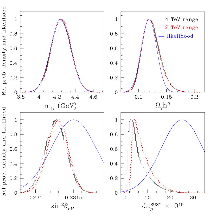
When combining many different constraints, it is possible that some combinations of them might be in conflict with each other. This has been mentioned above for $\delta a_{\mu}^{\text{SUSY}}$, where we remarked that the posterior pdf tends to prefer a value close to zero. This is further highlighted in Fig. 10 for a few representative cases. For each observable, we plot the 1–dimensional marginalized posterior pdf for the two prior ranges, along with the Gaussian likelihood function used in the analysis. If all the observations agreed with each other and in the absence of strong correlation among variables, we would expect the posterior pdf and the likelihood to overlap. This is the case for example for the bottom mass $m_{b}(m_{b})^{\overline{MS}}$ and for $\Omega_{\chi}h^{2}$ (upper panels). In the latter case, the slightly skewed shape of the posterior is due to our treatment of the theoretical uncertainty, which is larger for larger values of $\Omega_{\chi}h^{2}$. However, the posterior pdf for ${\sin^{2}\theta_{\text{eff}}}$ and $\delta a_{\mu}^{\text{SUSY}}$ show a tension with the likelihood representing the experimental result. We see a “pull” in the posterior towards values of ${\sin^{2}\theta_{\text{eff}}}$ lower than the measured mean (about one standard deviation discrepancy). We notice a similar situation for $M_{W}$. This tension is even more pronounced for the SUSY contribution to the anomalous magnetic moment of the muon $\delta a_{\mu}^{\text{SUSY}}$, whose posterior pdf peaks at values close to zero, in contrast to the experimental measurement. This is a sign of a tension between the various constraints used, with the other measurements pulling the posterior pdf for $\delta a_{\mu}^{\text{SUSY}}$ towards the SM value. This motivates us to investigate the dependence of our results on the inclusion of the $\delta a_{\mu}^{\text{SUSY}}$ measurement, which will be presented in section 4.6.

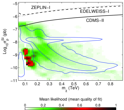
4.3 Mean quality of fit

In Bayesian statistics, the posterior pdf represents our state of knowledge about the parameters in the problem after we have seen the data and given our choice of priors, as we have explained in some detail in section 2.1. It is important to remark that regions of high posterior probability do not necessarily correspond to the best fitting points. The quality of fit is defined in terms of an effective $\chi^{2}$, obtained from the likelihood as

$$\chi^{2}(\theta)=-2\text{ ln}\,p\left(d|\xi(\theta)\right).$$ (36)

We can easily imagine a situation where a tiny multi–dimensional region in parameter space – let us call it a “spike” – shows an excellent quality of fit. At the same time, there might be another region where the quality of fit is slightly worse, but whose volume in parameter space is much larger. The much larger volume of the latter region gives it a higher weight, since it is more generic and hence less fine–tuned. In such a case, the posterior pdf would show a strong peak in the large region, while for the spike it would be suppressed due to its smallness. At the same time, the quality of fit statistics would show a stronger peak in the spike. We emphasize that this is not a feature of the MCMC exploration of parameter space, but rather a characteristics built into the Bayesian formalism. As a consequence, our inferences automatically give more weight to regions of parameter space showing less fine–tuning.

In the above scenario, an analysis performed using a fixed–grid scan and a quality of fit statistics would reach potentially very different conclusions. It can be shown, however, that both methods lead to the same conclusions if the data is informative enough, i.e., if their constraining power is sufficient. Conversely, a discrepancy between the posterior pdf and the quality of fit statistics is a useful indicator that the above mechanism is at work.

In order to carry out such a comparison, we compute the mean quality of fit in two dimensions. This is obtained from the posterior pdf by adopting the effective $\chi^{2}$ defined in Eq. (36) as a function of the parameters $f(\theta)$, as explained below Eq. (7), and plotting it in the dimensions of interest in parameter space. In Fig. 11 we plot the mean quality of fit in the same six panels for which we presented the posterior pdf in Fig. 2. The blue (solid) contours are the same as in Fig. 2 and are displayed to facilitate the comparison between the two quantities.

Figure 11: The quality of fit in the planes spanned by the CMSSM parameters: $m_{1/2}$, $m_{0}$, $A_{0}$ and $\tan\beta$ for the “4 TeV range” scan. This figure should be compared with Fig. 2 where the relative 2–dim joint relative probabilities are plotted for the same pairs of variables.

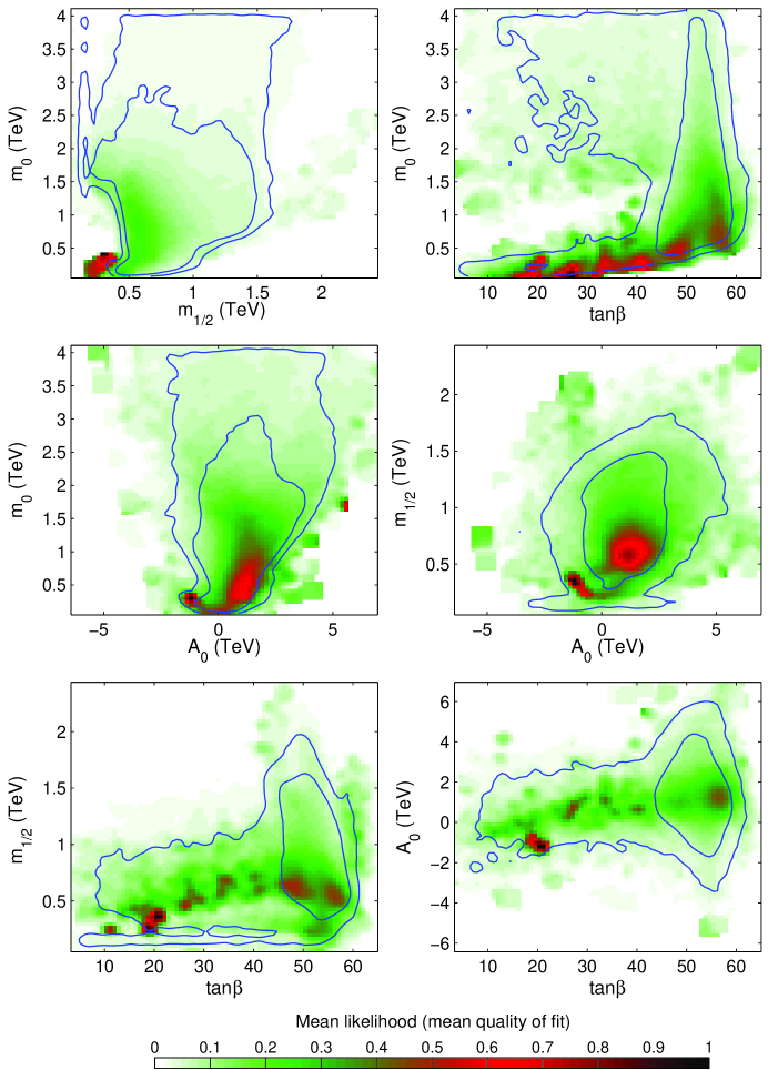
In some panels, the best fitting points (represented by dark red regions) are much more localized then the high–probability pdf. For example in the $(m_{1/2},m_{0})$ plane we find the best quality of fit in the region $m_{0},m_{1/2}\mathrel{\hbox to0.0pt{\lower 4.0pt\hbox{\hskip 1.0pt$\sim$}\hss}\raise 1.0pt\hbox{$<$}}0.5\mbox{ TeV}$. In the $(\tan\beta,m_{0})$ plane, on the other hand, we observe that good fitting point exist for almost all values of $\tan\beta$, down to $\tan\beta\approx 15$. Comparing with the corresponding panel in Fig. 2, we conclude that the strong preference for a large $\tan\beta$ shown by the posterior pdf does not imply that all the best fitting points lie in that region of parameter space. This issue can only be resolved once better data becomes available.

Figure 12: As in Fig. 6, but for $\sigma^{SI}_{p}$.

Figure 13: Top panel: the 2–dimensional relative probability density $p({m_{\chi}},{\sigma^{SI}_{p}}|d)$, with the contours containing 68% and 95% probability also marked. Bottom panel: the mean quality of fit (likelihood) with the same 68% and 95% probability contours as in the top panel to facilitate the comparison. Current 90% experimental upper limits are also shown.

4.4 Direct detection of DM

Predictions for $\sigma^{SI}_{p}$ are usually determined as a function of the CMSSM parameters by rigidly enforcing relevant constraints, e.g., 1 or $2\sigma$ ranges of $\Omega_{\chi}h^{2}$ or $BR({\bar{B}}\rightarrow X_{s}\gamma)$, etc. In our analysis, we present a posterior pdf which simultaneously accounts for all the constraints and sources of uncertainties.

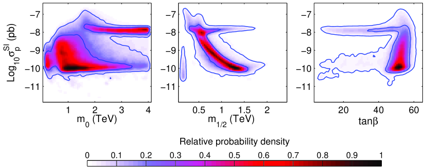
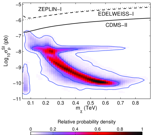
In Fig. 12 we plot the posterior pdf for the spin–independent elastic cross section $\sigma^{SI}_{p}$ and the CMSSM parameters $m_{0}$, $m_{1/2}$ and $\tan\beta$. In the left panel one can see three well–separated high probability regions. One is centered at $0.8\mbox{ TeV}\mathrel{\hbox to0.0pt{\lower 4.0pt\hbox{\hskip 1.0pt$\sim$}\hss}\raise 1.0pt\hbox{$<$}}m_{0}\mathrel{\hbox to0.0pt{\lower 4.0pt\hbox{\hskip 1.0pt$\sim$}\hss}\raise 1.0pt\hbox{$<$}}3\mbox{ TeV}$ and $\sigma^{SI}_{p}\simeq 10^{-10}\,\mbox{pb}$, although values almost as large as $10^{-8}\,\mbox{pb}$ are also allowed. It comes from the bulk, the stau coannihilation and the pseudoscalar resonance regions. To the left, and almost adjacent to it, there is a fairly narrow vertical band resulting from a light Higgs resonance mentioned above. The last main region is at large $m_{0}\mathrel{\hbox to0.0pt{\lower 4.0pt\hbox{\hskip 1.0pt$\sim$}\hss}\raise 1.0pt\hbox{$>$}}2\mbox{ TeV}$ and almost constant $\sigma^{SI}_{p}\simeq 1.6\times 10^{-8}\,\mbox{pb}$ which results from the FP region. Comparing with the right panel in Fig. 12 we can see that $\sigma^{SI}_{p}$ from the FP region and the light Higgs resonance are fairly independent of $\tan\beta$ while the bulk, coannihilation and resonance region requires large $\tan\beta$. Finally, the middle panel is added for completeness and it closely resembles the top panel of Fig. 13 (because $m_{\chi}\simeq 0.4m_{1/2}$) where we present the 2–dimensional pdf for $\sigma^{SI}_{p}$ and $m_{\chi}$. For comparison, we also show current CDMS–II, Edelweiss–I and UKDMC ZEPLIN–I 90% CL limits, but we stress that this constraint has not been used in the likelihood.

The features discussed above are visible in Fig. 13 (top). Firstly, the biggest, banana–shaped region of high probability ($68\%$ regions delimited by the internal solid, blue curve) shows a well–defined anti–correlation between $\sigma^{SI}_{p}$ and $m_{\chi}$. It comes from the bulk and stau coannihilation region (larger $\sigma^{SI}_{p}$) and from the $A$–resonance (smaller $\sigma^{SI}_{p}$) at large $\tan\beta$. This region covers roughly the range $10^{-10}\mathrel{\hbox to0.0pt{\lower 4.0pt\hbox{\hskip 1.0pt$\sim$}\hss}\raise 1.0pt\hbox{$<$}}\sigma^{SI}_{p}\mathrel{\hbox to0.0pt{\lower 4.0pt\hbox{\hskip 1.0pt$\sim$}\hss}\raise 1.0pt\hbox{$<$}}10^{-8}\,\mbox{pb}$ and $0.2\mbox{ TeV}\mathrel{\hbox to0.0pt{\lower 4.0pt\hbox{\hskip 1.0pt$\sim$}\hss}\raise 1.0pt\hbox{$<$}}m_{\chi}\mathrel{\hbox to0.0pt{\lower 4.0pt\hbox{\hskip 1.0pt$\sim$}\hss}\raise 1.0pt\hbox{$<$}}0.7\mbox{ TeV}$. In both cases the dominant contribution to $\sigma^{SI}_{p}$ typically comes from a heavy Higgs exchange.

Secondly, at small $m_{\chi}\mathrel{\hbox to0.0pt{\lower 4.0pt\hbox{\hskip 1.0pt$\sim$}\hss}\raise 1.0pt\hbox{$<$}}0.1\mbox{ TeV}$ we can again see a small vertical band of fairly low relative probability density ($\mathrel{\hbox to0.0pt{\lower 4.0pt\hbox{\hskip 1.0pt$\sim$}\hss}\raise 1.0pt\hbox{$<$}}0.2$) at small $\sigma^{SI}_{p}$. This region is allowed by the light Higgs resonance contribution to reducing $\Omega_{\chi}h^{2}$ at small $m_{1/2}$. This region essentially never features in usual fixed–grid scans, which do not smear out experimental bounds. This region would also disappear with a fair improvement in the lower bound on $m_{h}$.

Thirdly, we can see a well pronounced region of high relative probability at fairly constant $\sigma^{SI}_{p}\simeq 1.6\times 10^{-8}\,\mbox{pb}$ for $m_{\chi}\mathrel{\hbox to0.0pt{\lower 4.0pt\hbox{\hskip 1.0pt$\sim$}\hss}\raise 1.0pt\hbox{$<$}}0.42\mbox{ TeV}$ which at low $m_{\chi}$ partly overlaps with the previous region. At $95\%$ this region extends up to $m_{\chi}\mathrel{\hbox to0.0pt{\lower 4.0pt\hbox{\hskip 1.0pt$\sim$}\hss}\raise 1.0pt\hbox{$<$}}0.72\mbox{ TeV}$ for fairly constant $\sigma^{SI}_{p}$. This “high” $\sigma^{SI}_{p}$ band is a result of the FP region, basically independently of $\tan\beta$, as discussed above. This result has to be interpreted carefully, since there are large uncertainties associated with FP region, in particular with its location in the $(m_{1/2},m_{0})$ plane mentioned earlier. Hopefully, associated uncertainties in $\sigma^{SI}_{p}$ are going to be much smaller since it depends on low energy quantities like Higgs masses and the $\mu$ parameter. Despite those outstanding questions, we believe that it is probably safe to expect that the FP will be the first to be probed by DM search experiments.

Finally, after marginalizing over all other parameters, we obtain the following 1–dimensional regions encompassing 68% and 95% of the total probability:

$$1.0\times 10^{-10}\,\mbox{pb}<\sigma^{SI}_{p}<1.0\times 10^{-8}\,\mbox{pb} (68\%\text{ region}),$$ (37)

$$0.5\times 10^{-10}\,\mbox{pb}<\sigma^{SI}_{p}<3.2\times 10^{-8}\,\mbox{pb} (95\%\text{ region}).$$

Currently running experiments (most notably CDMS–II but also Edelweiss–II and ZEPLIN–II) should be able to reach down to a few $\times 10^{-8}\,\mbox{pb}$, on the edge of exploring the FP region. A future generation of “one–tonne” detectors are expected to reach down to $\sigma^{SI}_{p}\mathrel{\hbox to0.0pt{\lower 4.0pt\hbox{\hskip 1.0pt$\sim$}\hss}\raise 1.0pt\hbox{$>$}}10^{-10}\,\mbox{pb}$, thus exploring almost the whole $68\%$ region and much of the $95\%$ interval as well.

As discussed in section 4.3, the posterior pdf may be rather different from the mean quality of fit. In the bottom panel of Fig. 13 we plot the quality of fit (defined in Eq. (36)) for $\sigma^{SI}_{p}$ and $m_{\chi}$. The best fit points are found in the region $0.1\mbox{ TeV}\mathrel{\hbox to0.0pt{\lower 4.0pt\hbox{\hskip 1.0pt$\sim$}\hss}\raise 1.0pt\hbox{$<$}}m_{\chi}\mathrel{\hbox to0.0pt{\lower 4.0pt\hbox{\hskip 1.0pt$\sim$}\hss}\raise 1.0pt\hbox{$<$}}0.2\mbox{ TeV}$ and $1\times 10^{-10}\,\mbox{pb}\mathrel{\hbox to0.0pt{\lower 4.0pt\hbox{\hskip 1.0pt$\sim$}\hss}\raise 1.0pt\hbox{$<$}}\sigma^{SI}_{p}\mathrel{\hbox to0.0pt{\lower 4.0pt\hbox{\hskip 1.0pt$\sim$}\hss}\raise 1.0pt\hbox{$<$}}3\times 10^{-9}\,\mbox{pb}$, but other good fitting points (quality of fit about 0.4, dark green regions) lie right near the top of the high probability region, at rather large $\sigma^{SI}_{p}$.

4.5 Correlations among observables

Figure 14: The 2–dimensional relative probability density $p({\xi_{i}},{\xi_{j}}|d)$ for the pairs of observables marked along horizontal and vertical axes.

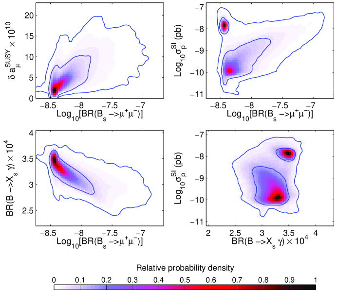
We now proceed to examine various correlations among the observables discussed above. In the upper left panel of Fig. 14 we show the 2–dimensional pdf for $BR(B_{s}\rightarrow\mu^{+}\mu^{-})$ and $\delta a_{\mu}^{\text{SUSY}}$. We can clearly see a rather strong correlation between those two variables [98] but, as pointed out above, the most probable ranges of both variables are on a low side. A positive measurement of $BR(B_{s}\rightarrow\mu^{+}\mu^{-})$ at the Tevatron (above some $2\times 10^{-8}$) would lead to a very strong tension with the current result for $\delta a_{\mu}^{\text{SUSY}}$.

In the upper right panel of Fig. 14 we show the 2–dimensional pdf for $BR(B_{s}\rightarrow\mu^{+}\mu^{-})$ and $\sigma^{SI}_{p}$. We can see two high relative probability regions here showing an interesting pattern. The one at smaller values of both variables comes from the coannihilation and Higgs resonance regions and has been pointed out in [99]. In addition, the FP region allows for a second “island” where $\sigma^{SI}_{p}$ is not far below the current CDMS limit while $BR(B_{s}\rightarrow\mu^{+}\mu^{-})$ is very small, far below the reach of the Tevatron. Thus, because of the FP region, a signal in measuring $\sigma^{SI}_{p}$ in current generation of DM search detectors would not necessarily imply a high probability of measuring $BR(B_{s}\rightarrow\mu^{+}\mu^{-})$ at the Tevatron, (or vice versa, contrary to the claim of [99]).

In the two bottom panels of Fig. 14 we show high probability regions for $BR(B_{s}\rightarrow\mu^{+}\mu^{-})$ and $BR({\bar{B}}\rightarrow X_{s}\gamma)$, and for $BR({\bar{B}}\rightarrow X_{s}\gamma)$ and $\sigma^{SI}_{p}$. In the first case, the high relative probability region for $BR(B_{s}\rightarrow\mu^{+}\mu^{-})$ lies at small values, just above the SM prediction and corresponds to the $BR({\bar{B}}\rightarrow X_{s}\gamma)$ around the central value, as noted above. It may eventually be possible to verify this correlation experimentally. Finally the variables $BR({\bar{B}}\rightarrow X_{s}\gamma)$ and $\sigma^{SI}_{p}$ show two separate peaks in the relative probability density. Again, the peak at smaller $\sigma^{SI}_{p}$ comes from the coannihilation and Higgs resonance regions while the other one from the FP region. In principle, a measurement of $\sigma^{SI}_{p}$ above some $10^{-8}\,\mbox{pb}$ would point towards a range of $BR({\bar{B}}\rightarrow X_{s}\gamma)$ above the current central value. Unfortunately, until a full NLO SUSY contribution is available, error bars in the latter quantity will remain at the level of some 10%, which would make it difficult to confirm the FP origin of the $\sigma^{SI}_{p}$ measurement.

Figure 15: Values of $m_{h}$ (upper left), $\Omega_{\chi}h^{2}$ (upper right), $\sigma^{SI}_{p}$ (lower left) and $\delta a_{\mu}^{\text{SUSY}}$ (lower right) in the $(m_{1/2},m_{0})$ plane for samples uniformly selected from our MC chains. While $\sigma^{SI}_{p}$ and $\delta a_{\mu}^{\text{SUSY}}$ show a clear correlation with the values of $(m_{1/2},m_{0})$, the CDM abundance $\Omega_{\chi}h^{2}$ can take any value within the $2\sigma$ WMAP range in the plane. Narrow “WMAP strips” in the $(m_{1/2},m_{0})$ plane for fixed values of $\tan\beta$ and $A_{0}$ thus disappear when these parameters are allowed to vary and all other parameters are correctly marginalized over.

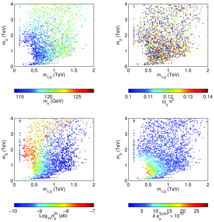
In the four panels of Fig. 15 we plot in the $(m_{1/2},m_{0})$ plane values of $m_{h}$ (upper left), $\Omega_{\chi}h^{2}$ (upper right), $\delta a_{\mu}^{\text{SUSY}}$ (lower left) and $\sigma^{SI}_{p}$ (lower right). The points have been drawn uniformly from our MC chains. To highlight the values of interest for the observables, the range of the color scales has been reduced, and points with values above (below) the scale have been plotted in red (blue). One can see that $m_{h}$ increases with increasing $m_{1/2}$ or $m_{0}$, as expected. In the region where $m_{1/2}\mathrel{\hbox to0.0pt{\lower 4.0pt\hbox{\hskip 1.0pt$\sim$}\hss}\raise 1.0pt\hbox{$<$}}1\mbox{ TeV}$ and/or $m_{0}\mathrel{\hbox to0.0pt{\lower 4.0pt\hbox{\hskip 1.0pt$\sim$}\hss}\raise 1.0pt\hbox{$<$}}2\mbox{ TeV}$ (roughly the reach of the LHC) one predominantly finds $m_{h}\mathrel{\hbox to0.0pt{\lower 4.0pt\hbox{\hskip 1.0pt$\sim$}\hss}\raise 1.0pt\hbox{$<$}}117\mbox{ GeV}$ (although larger values are not excluded), which is encouraging for Higgs searches [100]. In all the panels, at $m_{1/2}\simeq 0.2\mbox{ TeV}$, there is a vertical favored region due to a narrow light Higgs resonance contribution to $\Omega_{\chi}h^{2}$. It is interesting that in the rest of the $(m_{1/2},m_{0})$ plane one finds that the WIMP relic density (upper right window) can take any value within about the $2\sigma$ range of (21). In other words, even though for each particular choice of the CMSSM and nuisance SM parameters there are only a few narrow regions consistent with the DM constraint (19), by performing the appropriate marginalization over all other parameters it appears to be fairly easy to satisfy the WMAP value of the DM abundance at almost any point in the $(m_{1/2},m_{0})$ plane. This feature can also be seen in Fig. 6.

The values of $\sigma^{SI}_{p}$ (bottom left panel of Fig. 15) cover a large range but are generally larger for smaller $m_{1/2}$ and intermediate and large $m_{0}$ (compare with Figs. 12 and 13 (top)), with the exception of the light Higgs boson resonance region at small $m_{1/2}$. This means that DM direct detection searches will in general explore the large $m_{0}$ region of FP first – an interesting complementarity with collider searches.

On the other hand, the claimed discrepancy between experiment and the SM value (16) of the anomalous magnetic moment, when taken at face value, clearly points towards a different region of $m_{1/2}\mathrel{\hbox to0.0pt{\lower 4.0pt\hbox{\hskip 1.0pt$\sim$}\hss}\raise 1.0pt\hbox{$<$}}0.8\mbox{ TeV}$ (at small $m_{0}$) and $m_{0}\mathrel{\hbox to0.0pt{\lower 4.0pt\hbox{\hskip 1.0pt$\sim$}\hss}\raise 1.0pt\hbox{$<$}}1.5\mbox{ TeV}$ (at small $m_{1/2}$), as can be seen in the bottom right panel of Fig. 15. Thus, similarly to the case of $BR(B_{s}\rightarrow\mu^{+}\mu^{-})$ described above, a positive measurement of $\sigma^{SI}_{p}$ in currently running DM detectors (above some $2\times 10^{-8}\,\mbox{pb}$) would lead to a strong tension with the current result for $\delta a_{\mu}^{\text{SUSY}}$.

4.6 Sensitivity to $(g-2)_{\mu}$

Figure 16: The 1–dimensional relative posterior pdf’s as in Fig. 4. The black solid (blue dotted) line is for the analysis including (excluding) the measurement of the anomalous magnetic moment of the muon, Eq. (16). Both cases assume the “4 TeV range” priors.

Figure 17: As in Fig. 5. The black solid (blue dotted) line is for the analysis including (excluding) the measurement of the anomalous magnetic moment of the muon, Eq. (16). Both cases assume the “4 TeV range” priors.

Figure 18: The probability for the superpartner masses to lie below a given mass. All other parameters have been marginalized over.

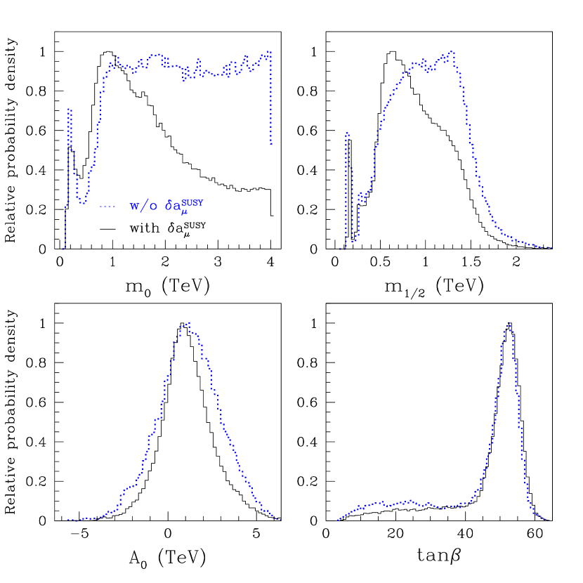
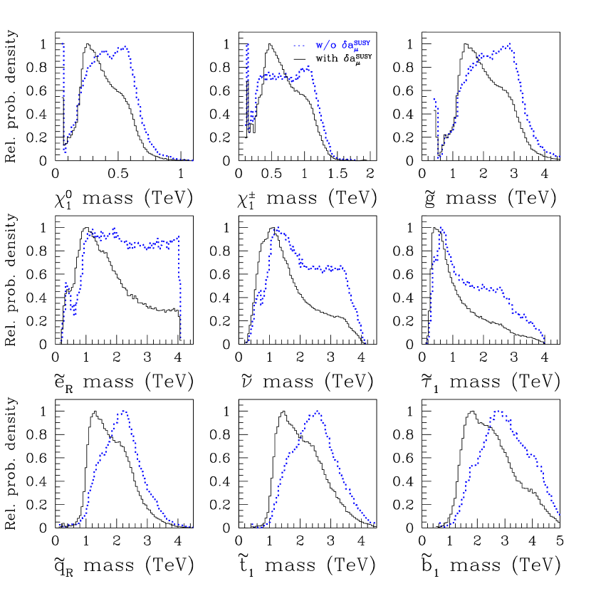
As we have shown above, the $2.7\sigma$ deviation of the anomalous magnetic moment of the muon from the SM prediction appears to be in tension with some of the other observables. To investigate to what extent our statistical inferences on superpartner masses rely on the inclusion of $\delta a_{\mu}^{\text{SUSY}}$, in this section we present the posterior pdf’s obtained by dropping it from the likelihood. To be as general as possible, we have adopted the “4 TeV range” of the priors.

Fig. 16 compares the 1–dimensional marginalized posterior pdf $p({\theta_{i}}|d)$, where $\theta_{i}=m_{0}$, $m_{1/2}$, $A_{0}$ and $\tan\beta$ with and without the inclusion of $\delta a_{\mu}^{\text{SUSY}}$ in the likelihood. If we drop the anomalous magnetic moment measurement we loose essentially all constraint on $m_{0}$, whose pdf becomes flat above $1\mbox{ TeV}$. The impact on $m_{1/2}$ is very mild, with a slight shift to larger values of the bulk of the pdf. There is also almost no change in the pdf’s for $A_{0}$ and $\tan\beta$. Intervals encompassing 68% and 95% of probability for the CMSSM parameters are given in Table 7 (compare with Table 5).

The implications for several representative superpartner masses are presented in Fig. 17, which should be compared with Fig. 5. The corresponding probability intervals are summarized in Table 8. One should remember that the dominant contribution to $\delta a_{\mu}^{\text{SUSY}}$ comes from the sneutrino–chargino exchange [101]. Since $m_{\widetilde{\nu}}$ depends much more strongly on $m_{0}$ than on $m_{1/2}$, while $m_{\chi_{1}^{\pm}}$ is more dependent on $m_{1/2}$, both soft parameters are affected but $m_{0}$ more strongly.

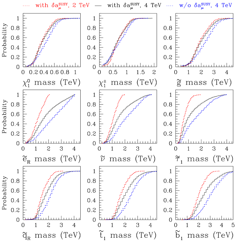
An experimental implication for the LHC is rather obvious. If the $\delta a_{\mu}^{\text{SUSY}}$ anomaly is not confirmed, the probability of finding sleptons and squarks will be reduced. This can be see in Fig. 18 where we plot the total probability as a function of mass for several superpartners. We show three cases: the “2 TeV range” (dotted red), as well as our default “4 TeV range” case with (black solid) and without (dotted blue) the $(g-2)_{\mu}$ constraint (16). It is clear that the total probability that the mass of squarks or sleptons lies below a certain value depends rather strongly on the choice priors and/or the $(g-2)_{\mu}$ constraint. On the other hand, this is not the case for the gauginos. By comparing Tables 8 and 6 it would seem that the upper bound of the 95% interval does not change much for the squark and gluino masses. However, this is probably a manifestation of the upper cut induced around 4 TeV by the prior, and therefore should not be taken as a robust result of the inference, analogously to what has been discussed above for $m_{0}$.

	“4 TeV range”, no $(g-2)_{\mu}$
Parameter	68% region	95% region
$m_{0}$ (TeV)	$<2.87$	$<3.85$
$m_{1/2}$ (TeV)	$(0.56,1.38)$	$(0.14,1.73)$
$A_{0}$ (TeV)	$(-0.60,2.89)$	$(-2.46,4.59)$
$\tan\beta$	$(28.2,53.8)$	$(10.2,57.0)$

Table 7: CMSSM parameter ranges corresponding to 68% and 95% of posterior probability (with all other parameters marginalized over) for the “4 TeV range” but without the constraint from $(g-2)_{\mu}$. These ranges should be compared with Table 5.

Super–	“4 TeV range”, no $(g-2)_{\mu}$
partner	68%	95%
$\chi_{1}^{0}$	$(0.23,0.60)$	$(0.57,0.76)$
$\chi_{1}^{\pm}$	$(0.33,1.10)$	$(0.11,1.31)$
$\widetilde{g}$	$(1.36,3.05)$	$(0.42,3.79)$
$\tilde{e}_{R}$	$(1.12,3.48)$	$(0.40,3.95)$
$\tilde{\nu}$	$(1.11,3.18)$	$(0.56,3.75)$
$\tilde{\tau}_{1}$	$(0.61,2.71)$	$(0.32,3.58)$
$\tilde{q}_{R}$	$(2.08,4.00)$	$(1.43,4.75)$
$\tilde{t}_{1}$	$(1.47,2.76)$	$(1.00,3.48)$
$\tilde{b}_{1}$	$(1.70,3.19)$	$(1.21,3.95)$

Table 8: Selected superpartner mass ranges (in TeV) containing 68% and 95% of posterior probability (with all other parameters marginalized) for the “4 TeV range” but without the constraint from $(g-2)_{\mu}$. These intervals should be compared with Table 6.

Observable	“4 TeV range”, with $(g-2)_{\mu}$		“4 TeV range”, w/o $(g-2)_{\mu}$
	68%	95%	68%	95%
$\Omega_{\chi}h^{2}$	$(0.107,0.138)$	$(0.946,0.157)$	$(0.107,0.138)$	$(0.949,0.158)$
$\delta a_{\mu}^{\text{SUSY}}\times 10^{10}$	$(1.9,9.9)$	$(0.8,17.1)$	N/A	N/A
$BR(B_{s}\rightarrow\mu^{+}\mu^{-})\times 10^{9}$	$(3.5,16.8)$	$(3.3,75.0)$	$(3.5,8.5)$	$(3.3,41.0)$
$BR({\bar{B}}\rightarrow X_{s}\gamma)\times 10^{4}$	$(2.93,3.44)$	$(2.62,3.61)$	$(3.08,3.49)$	$(2.77,3.62)$
$\sigma^{SI}_{p}(\,\mbox{pb}\times 10^{10})$	$(1,100)$	$(0.5,320)$	$(0.8,117)$	$(0.3,208)$

Table 9: Intervals encompassing 68% and 95% of posterior probability for selected observables (with all other parameters marginalized). The two columns compare results for the “4 TeV range” with (left column) and without (right column) inclusion of the constraint from $(g-2)_{\mu}$.

In Table 9 we summarize the effect of the $(g-2)_{\mu}$ constraint on some of our other observables. While the relic abundance is unaffected, $BR(B_{s}\rightarrow\mu^{+}\mu^{-})$ and $\sigma^{SI}_{p}$ get shifted to lower values as a consequence of a less constrained $m_{0}$ when the $(g-2)_{\mu}$ anomaly is discarded.

5 Summary and conclusions

In this work we performed a detailed investigation of the CMSSM parameter space using a MCMC method and analyzed our results in terms of Bayesian statistics. The power and flexibility of the approach allowed us to probe many previously unexplored ranges of parameters. Furthermore, we were able to improve on previous analyses in several important aspects. We fully incorporated the effects of remaining uncertainties in relevant SM parameters (including $\alpha_{\text{em}}(M_{Z})^{\overline{MS}}$), which are usually fixed to their central values. We incorporated often neglected theoretical uncertainties in computing mass spectra and observables. Finally, we improved upon the usual practice of applying sharp experimental limits and (typically) $1\sigma$ uncertainties by smearing them out.

By carefully constructing the likelihood function we constrained the CMSSM parameters by comparing several collider and astrophysical observables (except for $\sigma^{SI}_{p}$) with the available data. For all these variables we computed the posterior probability density functions – our main tool in analyzing our findings – in terms of which we delimited the favored regions of the CMSSM parameters, and further derived the ranges of the observables themselves that are favored by a combination of currently available data. We emphasized the difference between the posterior probability density and the quality of fit statistics. The latter is formulated in terms of an average effective $\chi^{2}$, and is akin to what is used in fixed–grid scans. For example, we concluded that the strong preference for a large $\tan\beta$ shown by the posterior pdf does not imply that all the best fitting points lie in that region of parameter space. This issue can only be resolved by acquiring better data.

We explored in detail the robustness and sensitivity of our results to the assumed initial ranges of CMSSM and SM parameters (priors). To this end we compared our findings for the default “4 TeV range” prior (which include the somewhat uncertain FP region) extending above the LHC reach, with the more restrictive “2 TeV range” prior. We emphasized that much care must be exercised in interpreting our inferences whenever boundaries of high probability regions lie close to the prior ranges. This applies mainly to $m_{0}$, and to the superpartner masses that primarily depend on it, while all other variables appear robust to a change in the range of the priors.

We furthermore examined various correlations among the relevant observables. Some have been pointed out before, e.g., between $BR(B_{s}\rightarrow\mu^{+}\mu^{-})$ and $\delta a_{\mu}^{\text{SUSY}}$ or $\sigma^{SI}_{p}$ (the last one showing a new feature due to the presence of the FP region). A more subtle correlation between $BR({\bar{B}}\rightarrow X_{s}\gamma)$ and $BR(B_{s}\rightarrow\mu^{+}\mu^{-})$ emerged, which may eventually be tested experimentally. We note that at present none of the observables appear to be in conflict with observations or with each other, with the possible exception of $(g-2)_{\mu}$. In particular, the cosmological constraint on $\Omega_{\chi}h^{2}$ appears less severe than what has been previously thought.

Our findings in the CMSSM strongly support the idea of low energy SUSY, although of course they do not disfavor other possibilities, like split SUSY [102]. Quantitatively, at 68% probability, we have found $0.52\mbox{ TeV}<m_{1/2}<1.26\mbox{ TeV}$, $m_{0}<2.10\mbox{ TeV}$, $-0.34\mbox{ TeV}<A_{0}<2.41\mbox{ TeV}$ and $38.5<\tan\beta<54.6$. The corresponding ranges of superpartner masses are given in column two of Table 6. A significant fraction of the 68% probability ranges of superpartner masses falls within the LHC reach, and typically outside the Tevatron reach. The same applies to $BR(B_{s}\rightarrow\mu^{+}\mu^{-})$ for which most favored CMSSM values are not far above the SM prediction. On the other hand, a positive measurement of $BR(B_{s}\rightarrow\mu^{+}\mu^{-})$ at the Tevatron would strongly disfavor large $m_{0}$, including the focus point region. The WIMP DM direct detection elastic scattering cross section $\sigma^{SI}_{p}$ shows a wide spread of values (below today’s limits) at around $10^{-9\pm 1}\,\mbox{pb}$ and a strong anti–correlation with $m_{\chi}$. In addition, a relatively large $\sigma^{SI}_{p}\simeq 1.6\times 10^{-8}\,\mbox{pb}$, fairly independent of $m_{\chi}$, appears to be a feature of the FP region (despite large theoretical uncertainties) and will probably be the first to be tested in direct detection experiments.

The $(g-2)_{\mu}$ anomaly still remaining the subject of some controversy, we re–examined its impact on the CMSSM parameter space. We showed the inference to be substantial on $m_{0}$, and any superpartner masses that primarily depend on it, while much less so with the other CMSSM parameters. The chance for the LHC to detect superpartners reduces somewhat but still remains strong.

Appendix A Markov chain Monte Carlo algorithm

A.1 Sampling

The purpose of the Markov Chain Monte Carlo (MCMC) algorithm is to construct a sequence of points in parameter space (called “a chain”) whose density is proportional to the posterior pdf of Eq. (5). Once such a chain has been produced, the posterior probability for a given region of parameter space (a bin) is obtained by simply counting the number of samples within that region. Marginalization over nuisance parameters (see Eq. (6)) is trivial: the coordinates of the parameters that one is not interested in are simply ignored when counting the samples.

Several algorithms are available to construct Markov chains, which are more or less suited to the structure of the parameter space under consideration, see e.g. [103] for an introductory review and references therein. We make use of the Metropolis algorithm: from a starting point in parameter space $\eta_{0}$ with associated posterior probability $p_{0}$, a candidate point $\eta_{c}$ for the next sample is proposed by sampling it from a transition probability $T(\eta_{0},\eta_{c})$. The candidate sample is then accepted with probability

$$\alpha=\min\left(\frac{p_{c}}{p_{0}},1\right),$$ (38)

where $p_{c}=p(\eta_{c}|d)$. Notice that all steps for which the candidate sample has a better probability than the previous one are accepted. If the candidate point is accepted, it becomes the new starting point, and another candidate is drawn. Otherwise the chain stays at the previous point (which is thus counted twice) and a new attempt is made from there. It can be shown that the sequence of samples $\eta_{0},\eta_{1},\dots,\eta_{t},\dots$ constructed this way converges to the target distribution $p(\eta|d)$ for $t\rightarrow\infty$.

The transition probability $T(\eta_{t},\eta_{t+1})$ must be symmetric in its arguments (so called “detailed balance”), a sufficient condition which ensures that the Markov chain constructed this way is sampling from the target probability distribution. In our case, the transition probability is given by the following prescription, which we found strikes a good balance between efficiency and robustness of the exploration. At each step, we alternatively update the value of the CMSSM parameters $\theta$ or of the nuisance parameters $\psi$. In general, all of the components of either $\theta$ or $\psi$ are updated at each step. The candidate point is proposed along the direction $w$, where the vector $w$ is restricted to either one of the two subspaces (CMSSM or nuisance parameters) and it is given by

$${w}={A}\cdot{u}.$$ (39)

Here, ${A}$ is a random rotation matrix which is restricted to a given subspace and which is renewed every 4 steps. The components of ${u}$ are initially chosen as a guess of the typical spread of the posterior distribution along each direction of parameter space. The results of a preliminary MCMC run are then used to estimate the covariance matrix for the posterior pdf, whose eigenvectors give directions of approximate degeneracies in the parameter space. In the final run, ${w}$ is built analogously as above, but this time by a random rotation in the space spanned by the projections of the eigenvectors of the covariance matrix. This procedure aims at aligning the directions of the proposals to degeneracy lines in parameter space, thus improving the efficiency of the MCMC walk.

Along the direction defined by ${w}$, the width of the step is chosen by multiplying $|{w}|$ by a scaling factor $s$ and a factor $r$ drawn from the distribution

$$p(r)\propto\frac{2}{3}r^{n-1}\exp(-nr^{2}/2)+\frac{1}{3}\exp(-r),$$ (40)

with $n=4$ and $s=2.4$. The first term on the rhs of the proposal distribution (40) tends to make the chain move away from $r=0$ for $n>1$, while the second term increases the probability near the origin. Thus this distribution tends to be robust even in situations where the target pdf is strongly non–Gaussian. The above choices for the proposal distribution and for the parameters $n,s$ are mostly a matter of trial–and–error. Our updating procedure follows closely the recommendations of [104]. Notice that since our choice of the step direction and size do not depend on $\eta_{t},\eta_{t+1}$ at any moment, the condition of detailed balance for the transition probability holds true.

A.2 Convergence

We start $N=12$ or $N=16$ chains in randomly chosen points of parameters space (within the boundary specified by our prior range), making sure that they lie well apart from each other in order to maximise the initial variance. A certain number of samples have to be discarded at the beginning of the chain, since the chain requires some time to equilibrate around the target distribution. This “burn–in period” is assessed by inspecting the evolution of the probability as a function of the number of samples. We find that discarding $10^{3}$ initial samples is more than sufficient.

The acceptance rate is defined as the percentage of accepted proposals. For the runs using the covariance matrix the typical acceptance rate is in the range $2-3\%$. This is rather low, compared to optimal cases where the acceptance rate is typically an order of magnitude larger. The reason for this is the configuration of the posterior pdf in multi–dimensional parameter space, which is strongly non–Gaussian and presents a challenging combination of wide regions and narrow wedges of high probability. There is no optimal strategy in this case, but we are confident that our chains have appropriately sampled the whole parameter space. We performed extensive checks by comparing runs obtained with and without the covariance matrix in order to make sure that the efficiency gain did not come at the expenses of a reduced sampling ability.

Mixing and convergence of the chains is assessed with the Gelman & Rubin R–statistics [105]. This represents the variance of the means divided by the mean of the variances between different chains. The usual criterion is that $R-1\mathrel{\hbox to0.0pt{\lower 4.0pt\hbox{\hskip 1.0pt$\sim$}\hss}\raise 1.0pt\hbox{$<$}}0.2$, but to be conservative we require that for our chains $R-1<0.05$ for all parameters (this means that our convergence criteria are more stringent).

Typically we run in parallel two sets of $N=12$ or $N=16$ chains, until each chain within the set has reached $3\times 10^{4}$ or $4\times 10^{4}$ samples (the exact numbers depending on the computing power available and on the convergence status). We check that each run has converged using the criterion outlined above, and we then perform consistency checks between the two runs. The final inferences are obtained after merging the two sets of chains together. At this final stage, the Gelman and Rubin criterion is again satisfied by the merged set consisting of $24\leq N\leq 32$ chains, containing a total number of samples in the range of $0.7\times 10^{6}$ to $1.3\times 10^{6}$.

References

- [1] G. L. Kane, C. F. Kolda, L. Roszkowski and J. D. Wells, Study of constrained minimal supersymmetry, Phys. Rev. D49 (1994) 6173 [arXiv:hep-ph/9312272].
- [2] P. Nath and R. Arnowitt, Phys. Rev. Lett. B74 (1995) 4592 [arXiv:hep-ph/9409301].
- [3] R. Roberts and L. Roszkowski, Implications for supersymmetry and grand unified and the neutrino relic abundance, Phys. Lett. B309 (1993) 329 [hep-ph/9301267].
- [4] L. Covi, J. E. Kim and L. Roszkowski, Axinos as cold dark matter, Phys. Rev. Lett. B82 (1999) 4180 [arXiv:hep-ph/9905212]; L. Covi, H. B. Kim, J. E. Kim and L. Roszkowski, Axinos as dark matter, 2001033 [arXiv:hep-ph/0101009]; L. Covi, L. Roszkowski, R. Ruiz de Austri and M. Small, Axino dark matter and the CMSSM, 2004003 [arXiv:hep-ph/0402240].
- [5] M. Bolz, W. Buchmüller and Plümacher, Baryon asymmetry and dark matter, Phys. Lett. B 443 (1998) 209 [arXiv:hep-ph/9809381]; M. Bolz, A. Brandenburg and W. Buchmüller, Thermal production of gravitinos, Nucl. Phys. B 606 (2001) 518 [arXiv:hep-ph/0012052]; J. R. Ellis, K. A. Olive, Y. Santoso and V. C. Spanos, Gravitino dark matter in the CMSSM, Phys. Lett. B588 (2004) 7 [arXiv:hep-ph/0312262]; J.L. Feng, A. Rajaraman and F. Takayama, Superweakly interacting massive particles, Phys. Rev. Lett. 91 (2003) 011302 [arXiv:hep-ph/0302215].
- [6] L. Roszkowski, R. Ruiz de Austri and K-Y. Choi, Gravitino dark matter in the CMSSM and implications for leptogenesis at the LHC, 2005080 [arXiv:hep-ph/0408227]; D. G. Cerdeno, K-Y. Choi, K. Jedamzik, L. Roszkowski and R. Ruiz de Austri, Gravitino dark matter in the CMSSM with improved constraints from BBN, arXiv:hep-ph/0509275.
- [7] T. Blazek, R. Dermisek and S. Raby, Predictions for the Higgs and supersymmetry spectra from SO(10) Yukawa unification with greater than 0 , Phys. Rev. Lett. B88 (2002) 111804 [arXiv:hep-ph/0107097]; Yukawa unification in SO(10), Phys. Rev. D65 (2002) 115004 [arXiv:hep-ph/0201081].
- [8] R. Dermisek, S. Raby, L. Roszkowski and R. Ruiz De Austri, Dark matter and SO(10) soft susy breaking, 20030304 [arXiv:hep-ph/0304101]; Dark matter and SO(10) soft susy breaking II, 20050509 [arXiv:hep-ph/0507233].
- [9] See, e.g., M. Drees and M. Nojiri, The neutralino relic density in minimal N=1 supergravity, Phys. Rev. D47 (1993) 376 [arXiv:hep-ph/9207234]; H. Baer and M. Brhlik, Cosmological relic density from minimal supergravity with implications for collider physics, Phys. Rev. D53 (1996) 597 [arXiv:hep-ph/9508321]; J. R. Ellis, T. Falk, K. A. Olive and M. Srednicki, Calculations of neutralino–stau coannihilation channels and the cosmologically relevant region of MSSM parameter space, Astropart. Phys. 13 (2000) 181 [Erratum-ibid. 15 (2001) 413 ] [arXiv:hep-ph/9905481]; J. R. Ellis, T. Falk, G. Ganis, K. A. Olive and M. Srednicki, The CMSSM parameter space at large tan beta, Phys. Lett. B510 (2001) 236 [arXiv:hep-ph/0102098]; T. Nihei, L. Roszkowski and R. Ruiz de Austri, New Cosmological and Experimental Constraints on the CMSSM, 2001024 [arXiv:hep-ph/0106334]; A. Lahanas and V. Spanos, Implications of the pseudo–scalar Higgs boson in determining the neutralino dark matter, Euro. Phys. Journ. C23 (2002) 185 [arXiv:hep-ph/0106345].
- [10] A. Lewis and S. Bridle, Cosmological parameters from CMB and other data: a Monte-Carlo approach, Phys. Rev. D66 (2002) 103511 [arXiv:astro-ph/0205436].
- [11] T. J. Loredo and D. Q. Lamb, Bayesian analysis of neutrinos observed from supernova SN 1987A, Phys. Rev. D65 (2002) 063002 [arXiv:astro-ph/0107260].
- [12] D. J. MacKay, Information theory, inference, and learning algorithms (CUP, 2003); E. T. Jaynes, Probability Theory. The logic of science, ed. G. L. Bretthorst, (CUP, 2003); P. C. Gregory, Bayesian Logical Data Analysis for the Physical Sciences (CUP, 2005). T. J. Loredo, From Laplace to Supernova SN 1987A: Bayesian Inference in Astrophysics, in “Maximum-Entropy and Bayesian Methods”, Dartmouth, 1989, Ed. P. Fougere (Dordrecht, The Netherlands: Kluwer Academic Publishers), 81–142 (1990).
- [13] S. Profumo and C.E. Yaguna, Statistical analysis of supersymmetric dark matter in the MSSM after WMAP, Phys. Rev. D70 (2004) 095004 [arXiv:hep-ph/0407036].
- [14] J. R. Ellis, K. A. Olive, Y. Santoso and V. C. Spanos, Likelihood analysis of the CMSSM parameter space, Phys. Rev. D69 (2004) 095004 [arXiv:hep-ph/0310356].
- [15] J. R. Ellis, S. Heinemeyer, K. A. Olive and G. Weiglein, Indirect sensitivities to the scale of supersymmetry, 2005013 [arXiv:hep-ph/0411216].
- [16] E. A. Baltz and P. Gondolo, Markov chain monte carlo exploration of minimal supergravity with implications for dark matter, 2004052 [arXiv:hep-ph/0407039].
- [17] B. C. Allanach and C. G. Lester, Multi–dimensional MSUGRA likelihood maps, arXiv:hep-ph/0507283.
- [18] B. C. Allanach, Naturalness priors and fits to the constrained minimal supersymmetric standard model, arXiv:hep-ph/0601089.
- [19] J. L. Feng, K. T. Matchev and T. Moroi, Multi–TeV scalars are natural in minimal supergravity ?, Phys. Rev. Lett. B84 (2000) 2322 [arXiv:hep-ph/9908309]; Focus Points and naturalness in supersymmetry, Phys. Rev. D61 (2000) 075005 [arXiv:hep-ph/9909334]; J. L. Feng, K. T. Matchev and F. Wilczek, Neutralino dark matter in focus point supersymmetry, Phys. Lett. B482 (2000) 388 [arXiv:hep-ph/0004043].
- [20] R. Trotta, Applications of bayesian model selection to cosmological parameters, arXiv: astro-ph/0504022.
- [21] L. S. Stark, P. Hafliger, A. Biland and F. Pauss, New allowed MSUGRA parameter space from variations of the trilinear scalar coupling , 2005059 [arXiv:hep-ph/0502197].
- [22] The ALEPH, DELPHI, L3 and OPAL Collaborations and the LEP Working Group for Higgs boson searches, R. Barate et al., Phys. Lett. B565 (2003) 61 [arXiv:hep-ex/0306033]; lephiggs.web.cern.ch/LEPHIGGS.
- [23] V. D. Barger, M. S. Berger and P. Ohmann, The supersymmetric particle spectrum, Phys. Rev. D49 (1994) 4908 [arXiv:hep-ph/9311269].
- [24] The Tevatron Electroweak Working Group. Combination of CDF and DØ results on top-quark mass, arXiv:hep-ex/0507091.
- [25] A. X. El–Khadra and M. Luke, The mass of the b quark, Ann. Rev. Nucl. Part. Sci. C52 (2002) 201 [arXiv:hep-ph/0208114].
- [26] S. Eidelman et al.[Particle Data Group Collaboration], Phys. Lett. B592 (2004) 1.
- [27] See lepewwg.web.cern.ch/LEPEWWG.
- [28] A. Pineda and A. Signer, Renormalization group improved sum rule analysis for the bottom quark mass, arXiv:hep-ph/0601185.
- [29] B. C. Allanach, SOFTSUSY: a C++ program for calculating supersymmetric spectra, Comput. Phys. Commun. C143 (2002) 305 [arXiv:hep-ph/0104145].
- [30] The Muon g-2 Collaboration, Measurement of the negative muon anomalous magnetic moment to 0.7 ppm, Phys. Rev. D92 (2004) 161802 [arXiv:hep-ex/0401008].
- [31] A. Hocker, The hadronic contribution to , arXiv:hep-ph/0410081.
- [32] Heavy Flavour Averaging Group, http://www.slac.stanford.edu/xorg/hfag.
- [33] The CDMS Collaboration, Limits on spin–independent WIMP-nucleon interactions from the two-tower run of the Cryogenic Dark Matter Search, arXiv: astro-ph/0509259.
- [34] LEP SUSY Working Group for the ALEPH, DELPHI, L3 and OPAL collaborations, http://lepsusy.web.cern.ch/lepsusy.
- [35] A. Heister et al.[ALEPH Collaboration], Search for scalar leptons collisions at center–of–mass energies up to , Phys. Lett. B526 (2002) 206 [arXiv:hep-ex/0112011].
- [36] P. Achard et al.[L3 Collaboration], Search for scalar leptons and scalar quarks at LEP, Phys. Lett. B580 (2004) 37 [arXiv:hep-ex/0310007].
- [37] A. Heister et al.[ALEPH Collaboration], Absolute mass lower limit for the lightest neutralino of the MSSM from data at up to , Phys. Lett. B583 (2004) 247.
- [38] J. Abdallah et al.[DELPHI Collaboration], Searches for supersymmetric particles in collisions up and interpretation of the results within the MSSM, Euro. Phys. Journ. C31 (2004) 421 [arXiv:hep-ex/0311019].
- [39] DØ Collaboration, http://www-d0.fnal.gov/Run2Physics.
- [40] D. M. Pierce, J. A. Bagger, K. T. Matchev and R-J. Zhang, Precision corrections in the minimal supersymmetric standard model, Nucl. Phys. B491 (1997) 3 [arXiv:hep-ph/9606211].
- [41] S. Heinemeyer and G. Weiglein, The MSSM in the light of precision data, arXiv:hep-ph/0307177.
- [42] A. Dedes, A. B. Lahanas and K. Tamvakis, The effective weak mixing angle in the MSSM, Phys. Rev. D59 (1999) 015019 [arXiv:hep-ph/9801425].
- [43] T. Moroi, The muon anomalous magnetic dipole moment in the minimal supersymmetric standard model, Phys. Rev. D53 (1996) 6565 [Erratum-ibid. D 56 (1997) 4424 ] [arXiv:hep-ph/9512396].
- [44] G. Degrassi and G. F. Giudice, QED logarithms in the electroweak corrections to the muon anomalous magnetic moment, Phys. Rev. D58 (1998) 053007 [arXiv:hep-ph/9803384].
- [45] S. Heinemeyer, D. Stǒckinger and G. Weiglein, Two loop SUSY corrections to the anomalous magnetic moment of the muon, Nucl. Phys. B690 (2004) 62 [arXiv:hep-ph/0312264].
- [46] S. Heinemeyer, D. Stǒckinger and G. Weiglein, Electroweak and supersymmetric two–loop corrections to , Nucl. Phys. B699 (2004) 103 [arXiv:hep-ph/0405255].
- [47] S. Heinemeyer, W. Hollik and G. Weiglein, Electroweak precision observables in the minimal supersymmetric standard model, arXiv:hep-ph/0412214.
- [48] M. Davier, S. Eidelman, A. Hocker and Z. Zhang, Updated estimate of the muon magnetic moment using revised results from annihilation, Euro. Phys. Journ. C31 (2003) 503 [arXiv:hep-ph/0308213].
- [49] P. Gambino and M. Misiak, Quark mass effects in , Nucl. Phys. B611 (2001) 338 [arXiv:hep-ph/0104034]; A. Ali, talk given at ICHEP04, Beijing, August 2004, to appear in the proceedings, see ichep04.ihep.ac.cn/db/paper.php.
- [50] C. Degrassi, P. Gambino and G. F. Giudice, in supersymmetry: large contributions beyond the leading order, 2000009 [arXiv:hep-ph/0009337].
- [51] P. Gambino and M. Misiak, Quark mass effects in , Nucl. Phys. B611 (2001) 338 [arXiv:hep-ph/0104034].
- [52] K. Okumura and L. Roszkowski, Deconstraining supersymmetry from , Phys. Rev. Lett. B92 (2004) 161801 [arXiv:hep-ph/0208101]; Large beyond leading order effects in in supersymmetry with general flavour mixing, 2003024 [arXiv:hep-ph/0308102].
- [53] J. Foster, K. Okumura and L. Roszkowski, New Higgs effects in B–physics in supersymmetry with general flavour mixing, Phys. Lett. B609 (2005) 102 [arXiv:hep-ph/0410323]; Probing the flavour structure of supersymmetry breaking with rare B–processes: a beyond leading order analysis, 2005094 [arXiv:hep-ph/0506146].
- [54] J. Foster, K. Okumura and L. Roszkowski, Current and future limits on general flavor violation in transitions in minimal supersymmetry, arXiv:hep-ph/0510422.
- [55] P. Gambino, U. Haisch and M. Misiak, Determining the sign of the amplitude, Phys. Rev. Lett. B94 (2005) 061803 [arXiv:hep-ph/0410155].
-
[56]
C. L. Bennett et al., First year Wilkinson microwave anisotropy probe (WMAP)
observations: preliminary maps and basic results, Astrophys. J. Suppl. 148 (2003) 1
[arXiv:astro-ph/0302207];
D. N. Spergel et al., First year Wilkinson microwave anisotropy probe (WMAP) observations: determination of cosmological parameters, ibid. 175 [arXiv:astro-ph/0302209];
L. Verde et al., First year Wilkinson microwave anisotropy probe (WMAP) observations: parameter estimation methodology, ibid. 195; [arXiv:astro-ph/0302218]. - [57] A. C. S . Readhead et al., Extended mosaic observations with the cosmic background imager, Astrophys. J. 609 (2004) 498 [arXiv:astro-ph/0402359].
- [58] C. Dickinson et al., High sensitivity measurements of the CMB power spectrum with the extended very small array, arXiv:astro-ph/0402498.
- [59] J. H. Goldstein et al., Estimates of cosmological parameters using the CMB angular power spectrum of ACBAR, Astrophys. J. 599 (2003) 773 [arXiv:astro-ph/0212517].
- [60] M. Tegmark et al., The 3–D power spectrum of galaxies from the SDSS, Astrophys. J. 606 (2004) 702 [arXiv:astro-ph/0310725].
- [61] W. L. Freedman et al., Final results from the Hubble space telescope key project to measure the Hubble constant, Astrophys. J. 553 (2001) 47 [arXiv:astro-ph/0012376].
- [62] A. G. Riess et al., Type IA supernovae discoveries at from the Hubble space telescope: evidence for past deceleration and constraints on dark energy evolution, Astrophys. J. 607 (2004) 665 [arXiv:astro-ph/0402512].
[63]
T. Nihei, L. Roszkowski and R. Ruiz de Austri,
Towards an accurate calculation of the neutralino relic density,
2001063 [arXiv:hep-ph/0102308];
T. Nihei, L. Roszkowski and R. Ruiz de Austri, Exact cross sections for the neutralino WIMP pair–annihilation, 2002031 [arXiv:hep-ph/0202009]. - [64] J. Edsjo and P. Gondolo, Neutralino relic density including coannihilations, Phys. Rev. D56 (1997) 1879 [arXiv:hep-ph/9704361].
- [65] T. Nihei, L. Roszkowski and R. Ruiz de Austri, Exact cross sections for the neutralino slepton coannihilation, 2002024 [arXiv:hep-ph/0206266].
- [66] J. R. Ellis, K. A. Olive and Y. Santoso, Calculations of neutralino stop coannihilations in the CMSSM, Ann. Phys. 18 (2003) 395 [arXiv:hep-ph/0112113].
- [67] P. Gondolo, J. Edsjo, P. Ullio, L. Bergstrom, M. Schelk and E. A. Baltz, DARKSUSY: computing supersymmetric dark matter properties numerically, http://www.physto.se/edsjo/darksusy/.
- [68] P. Gondolo and G. Gelmini, Cosmic abundances of stable particles: improved analysis, Nucl. Phys. B360 (1991) 145.
- [69] B. C. Allanach, S. Kraml and W. Porod, Theoretical uncertainties in sparticle mass predictions from computational tools, 2003016 [arXiv:hep-ph/0302102].
- [70] A. Djouadi, M. Spira and P.M. Zerwas, QCD corrections to hadronic Higgs decays, Z. Phys. C70 (1996) 427 [arXiv:hep-ph/9511344].
- [71] B. C. Allanach, G. Bélanger, F. Boudjema and A. Pukhov, Requirements on collider data tom match the precision of WMAP on supersymmetric dark matter, 2004020 [arXiv:hep-ph/0410091]; G. Bélanger, S. Kraml and A. Pukhov, Comparison of SUSY spectrum calculations and impact on the relic density constraints from WMAP, Phys. Rev. D72 (2005) 015003 [arXiv:hep-ph/0502079].
- [72] See, e.g., K. Griest, Calculations of rates for direct detection of neutralino dark matter, Phys. Rev. Lett. B61 (1988) 666; V. A. Bednyakov, H. V. Klapdor–Kleingrothaus and S. Kovalenko, On SUSY dark matter detection with spinless nuclei, Phys. Rev. D50 (1994) 7128 [arXiv:hep-ph/9401262]; L. Bergstrom and P. Gondolo, Limits on direct detection of neutralino dark matter from decays, Astropart. Phys. 5 (1996) 263 [arXiv:hep-ph/9510252]; J. R. Ellis, A. Ferstl and K. A. Olive, Exploration of elastic scattering rates for supersymmetric dark matter, Phys. Rev. D63 (2001) 065016 [arXiv:hep-ph/0007113]; E. Accomando, R. Arnowitt, B. Dutta and Y. Santoso, Neutralino proton cross-sections in supergravity models, Nucl. Phys. B585 (2000) 124 [arXiv:hep-ph/0001019]; A. Bottino, F. Donato, N. Fornengo and S. Scopel, Probing the supersymmetric parameter space by WIMP direct detection, Phys. Rev. D63 (2001) 125003 [arXiv:hep-ph/0010203]; M. E. Gomez and J. D. Vergados, Cold dark matter detection in SUSY models at large tan beta, Phys. Lett. B512 (2001) 252 [arXiv:hep-ph/0012020]; J. R. Ellis, A. Ferstl, K. A. Olive and Y. Santoso, Direct detection of dark matter in the MSSM with nonuniversal Higgs masses, Phys. Rev. D67 (2003) 123502 [arXiv:hep-ph/0302032]; H. Baer, C. Balazs, A. Belyaev and J. O’Farrill, Direct detection of dark matter in supersymmetric models, JCAP 0309 (007) 2003 [hep-ph/0305191]; D. G. Cerdeño, C. Hugonie, D. E. Lopez–Fogliani, C. Muñoz and A. M. Teixeira, Theoretical predictions for the direct detection of neutralino dark matter in the NMSSM, 0482004 [hep-ph/0408102]; J. R. Ellis, K. A. Olive, Y. Santoso and V. C. Spanos, Update on the direct detection of supersymmetric dark matter, Phys. Rev. D71 (095007) 2005 [hep-ph/0502001].
- [73] D. S. Akerib, et al., [CDMS Collaboration], First results from the cryogenic dark matter search in the Soudan underground lab., Phys. Rev. Lett. B93 (2004) 211301, [arXiv:astro-ph/0405033].
- [74] V. Sanglard et al.[EDELWEISS Collaboration], Final results of the EDELWEISS–I dark matter search with cryogenic heat–and–ionization Ge detectors, Phys. Rev. D71 (2005) 122002 [arXiv:astro-ph/0503265].
- [75] G. J. Alner et al.[UK Dark Matter Collaboration], First limits on nuclear recoil events from the ZEPLIN–I galactic dark matter detector, Astropart. Phys. 23 (2005) 444.
- [76] B. Moore, S. Ghigna, F. Governato, G. Lake, T. Quinn, J. Stadel and P. Tozzi, Dark matter substructure within galactic halos, Astropart. J. 524 (1999) 19; A. W. Graham, D. Merritt, B. Moore, J. Diemand and B. Terzic, Empirical models for dark matter halos, arXiv:astro-ph/0509417.
- [77] M. Drees and M. Nojiri, Neutralino–nucleon scattering revised, Phys. Rev. D48 (1993) 3483 [arXiv: hep-ph/9307208].
- [78] For a review, see, e.g., G. Jungman, M. Kamionkowski and K. Griest, Supersymmetric dark matter, Phys. Rep. 267 (1996) 195.
- [79] H. Baer and M. Brhlik, Neutralino dark matter in minimal supergravity: direct detection versus collider searches, Phys. Rev. D57 (1998) 567 [arXiv:hep-ph/9706509].
- [80] J. Ellis, A. Ferstl and K. A. Olive, Reevaluation of the elastic scattering of supersymmetric dark matter, Phys. Lett. B481 (2000) 304 [arXiv:hep-ph/0001005].
- [81] Y. G. Kim, T. Nihei, L. Roszkowski and R. Ruiz de Austri, Upper and lower limits on neutralino WIMP mass and spin–independent scattering cross section, and impact of new measurement, 2002034, [arXiv:hep-ph/0208069].
- [82] See http://user.pa.msu.edu/wkt/cteq/cteq6/cteq6pdf.html.
- [83] A. Bottino, F. Donato, N. Fornengo and S. Scopel, Implications for relic neutralinos of the theoretical uncertainties in the neutralino nucleon cross–section, Ann. Phys. 13 (2000) 215 [arXiv:hep-ph/9909228].
- [84] V. M. Abazov et al.[DØ Collaboration], A search for the flavor–changing neutral current decay in collisions at with the DØ detector, Phys. Rev. Lett. B94 (2005) 071802 [arXiv:hep-ex/0410039].
- [85] D. Acosta et al.[CDF Collaboration], Search for and decays in collisions with CDF II, Phys. Rev. Lett. B95 (2005) 221805 [Erratum-ibid. 95 (2005) 249905 ] [arXiv:hep-ex/0508036].
- [86] See DØ web page http://www-d0.fnal.gov/Run2Physics/WWW/results/prelim/B/B21/B21.pdf, V. M. Abazov et al.[DØ Collaboration], Update of the Upper Limit on the Rare Decay with the DØ Detector.
- [87] R. Bernhard et al.[CDF and DØ Collaborations], A combination of CDF and DØ limits on the branching ratio of decays, arXiv:hep-ex/0508058.
- [88] See, e.g., http://www-cdf.fnal.gov/physics/projections/.
- [89] A. J. Buras, Relations between and in models with minimal flavor violation, Phys. Lett. B566 (2003) 115 [arXiv:hep-ph/0303060].
- [90] C. Bobeth, T. Ewerth, F. krüger and J. Urban, Analysis of neutral Higgs–boson contributions to the decays and , Phys. Rev. D64 (2001) 074014 [arXiv:hep-ph/0104284].
- [91] M. Carena, D. Garcia, U. Nierste and C. E. Wagner, Effective Lagrangian for the interaction in the MSSM and charged Higgs phenomenology, Nucl. Phys. B577 (2000) 88 [arXiv:hep-ph/9912516].
- [92] J. R. Ellis, K. A. Olive and V. C. Spanos, On the interpretation of in the CMSSM, Phys. Lett. B624 (2005) 47 [arXiv:hep-ph/0504196].
- [93] C. Bobeth, A. J. Buras, F. Kruger and J. Urban, QCD corrections to , , and in the MSSM, Nucl. Phys. B630 (2002) 87 [arXiv:hep-ph/0112305].
- [94] B. C. Allanach, A. Djouadi, J. L. Kenur, W. Porod and P. Slavich, Precise determination of the neutral Higgs boson masses in the MSSM, 2004044 [arXiv:hep-ph/0406166].
- [95] S. Heinemeyer, W. Hollik, H. Rzehak and G. Weiglein, Higgs–precision predictions for the MSSM Higgs sector at , Euro. Phys. Journ. C39 (2005) 465 [arXiv:hep-ph/0411114].
[96]
J. Edsjo, M. Schelke, P. Ullio and P. Gondolo,
Accurate relic densities with neutralino,
chargino and sfermion coannihilations in mSUGRA,
JCAP 0304 (2003) 001 [arXiv:hep-ph/0301106];
J. R. Ellis, K. A. Olive and Y. Santoso, Calculations of neutralino stop coannihilation in the CMSSM, Astropart. Phys. 18 (2003) 395 [arXiv:hep-ph/0112113];
G. Bélanger, F. Boudjema, A. Cottrant, A. Pukhov and A. Semenov, WMAP constraints on SUGRA models with non–universal gaugino masses and prospects for direct detection, Nucl. Phys. B706 (2005) 411 [arXiv:hep-ph/0407218]. - [97] T. Nihei, L. Roszkowski and R. Ruiz de Austri, New Cosmological and Experimental Constraints on the CMSSM, 2001024 [arXiv:hep-ph/0106334].
- [98] A. Dedes, H. K. Dreiner and U. Nierste, Correlation of and in minimal supergravity, Phys. Rev. Lett. B87 (2001) 251804 [arXiv:hep-ph/0108037].
- [99] S. Baek, Y. G. Kim and P. Ko, Neutralino dark matter scattering and in SUSY models, 2005067 [arXiv:hep-ph/0406033].
- [100] For a recent study see, e.g., M. Carena, S. Heinemeyer, C. E. M. Wagner and G. Weiglein, MSSM Higgs boson searches at the Tevatron and the LHC: impact of different benchmark scenarios, arXiv:hep-ph/0511023.
- [101] U. Chattopadhyay and P. Nath, Probing supergravity grand unification in the Brookhaven g-2 experiment, Phys. Rev. D53 (1996) 1648 [arXiv:hep-ph/9507386].
- [102] N. Arkani-Hamed, S. Dimopoulos, G. F. Giudice and A. Romanino, Aspects of split supersymmetry, Nucl. Phys. B709 (2005) 3 [arXiv:hep-ph/0409232].
- [103] R. M. Neal, e.g., Technical Report CRG-TR-93-1, Dept. of Computer Science, University of Toronto, available from http://www.cs.utoronto.ca/radford/.
- [104] S. Bridle and A. Lewis, cosmomc package, available from cosmologist.info.
- [105] A. Gelman and D. Rubin, Inference from iterative simulations using multiple sequences, Statistical Science 7, 457-511 (1992).