Incorporating Memory Effects in Phase Separation Processes

Abstract

We consider the modification of the Cahn-Hilliard equation when a time delay process through a memory function is taken into account. We then study the process of spinodal decomposition in fast phase transitions associated with a conserved order parameter. Finite-time memory effects are seen to affect the dynamics of phase transition at short times and have the effect of delaying, in a significant way, the process of rapid growth of the order parameter that follows a quench into the spinodal region. These effects are important in several systems characterized by fast processes, like nonequilibrium dynamics in the early universe and in relativistic heavy-ion collisions.

keywords: nonequilibrium field dynamics, memory effects, relativistic heavy-ion collisions

The dynamics of phase transitions depends on whether the order parameter that characterizes the different phases of a system is a conserved quantity or not. In different fields of physics and chemistry the dynamics of a conserved order parameter has been described phenomenologically by the Cahn-Hilliard (CH) equation CH (see also Ref. bray-gunton for a review). However, it is a first order equation in time and as such does not take into account memory effects (ME), which may have quite important consequences on non-equilibrium dynamics for fast phase transitions.

The CH equation is a diffusion-reaction type of equation. Diffuse processes are characterized by microscopic scattering events. The diffusion equation, in particular, describes the limiting situation where the time between the scattering events is infinitesimally short and therefore does not respect causality. Since in real systems scattering events proceed through finite time intervals, their description through diffusion-type of equations poses serious problems in real physical situations, as already recognized for a very long time Jou1 . Another related problem with the usual diffusion equation is that it also leads to the breaking of the f-sum rule which gives the frequency sum of the dynamic structure factor Kadanoff ; Koidediff . However, when the time scales of the ME are much smaller than any other scales, the breaking of causality and its effects become negligible, like in several applications with the CH equation, particularly in problems of metallurgy (see for example the references in Cahn ).

However, memory and causality constrains cannot be ignored when the typical microscopic time scales are large in comparison with the other time scales characterizing the dynamics. Fast phase transitions are expected to have happened in the early universe and most certainly also characterize the phase transitions expected to occur in the highly excited matter formed in relativistic heavy-ion collisions (RHIC). In the early universe such situations may have happened when the typical microscopic time scales for relaxation, given by the inverse of the decay width associated with particle dynamics, is larger than the Hubble time. This is a situation likely to be expected when describing GUT phase transitions or even the inflationary dynamics Rudnei . In RHIC one expects to learn about the QCD phase transition Greiner ; KoideM . For instance, from the hydrodynamic analysis of the freeze-out temperature in the most central Au-Au collisions at 130 A GeV, the typical reaction time is around 10-20 fm/c Hama . However, the characteristic time scale of the memory function in the Langevin equation which describes the dynamics near the chiral phase transition is predicted to be about 1 fm/c (as, for example, it is shown in Fig. 4 of Ref. KoideM ), which is not short enough to be ignored. These are examples that, when analyzing e.g. the detailed dynamics related to conserved charges, may require the use of a related CH equation for these conserved charges that goes beyond the linear order in the time derivative and where ME can be accounted for.

In order to motivate causality in the CH equation, it is useful to start our discussion by briefly reviewing the introduction of ME in the diffusion equation. Consider a random walk process, described by the simplest Langevin equation, $\dot{x}(t)=\xi(t)$, where $\xi(t)$ represents a noise term with correlations $\langle\xi(t)\rangle=0$ and $\langle\xi(t)\xi(t^{\prime})\rangle=2\Gamma W(t-t^{\prime})$, with the intensity of the noise $\Gamma$. It is common to ignore ME and assume a Gaussian white noise, for which $W(t-t^{\prime})=\delta(t-t^{\prime})$. Then, the corresponding Fokker-Planck equation for the probability distribution $P(x,t)$ is the usual diffusion equation. However, if one takes ME into account through a colored noise, for example of the form $W(t-t^{\prime})=\exp(-|t-t^{\prime}|/\gamma)/\gamma$, one obtains the so-called causal diffusion equation, which can be approximated by the partial differential equation

$$\gamma\frac{\partial^{2}}{\partial t^{2}}P(x,t)+\frac{\partial}{\partial t}P(x,t)=\Gamma\,\nabla^{2}P(x,t).$$ (1)

The propagation speed of the equation is defined by $\sqrt{\Gamma/\gamma}$ and one can easily see that the propagation speed of the ordinary diffusion equation ($\gamma=0$) is infinite. A causal diffusion equation like Eq. (1) has been used recently gavin to discuss the evolution of conserved charges in RHIC. In the present paper we apply these ideas to dynamic phase transitions involving a conserved order parameter by deriving an analogous CH equation using memory functions. To the best of our knowledge, this is the first numerical analysis to incorporate memory constraints in a CH equation.

Though our primary motivations are fast phase transitions in cosmology and heavy-ion collision dynamics, we here adopt a very general approach that can also be of relevance in other applications, like in condensed matter systems. We shall then consider the following general Ginzburg-Landau (GL) free energy

$${}F(\phi)=\int d^{3}{\bf x}\left[\frac{a}{2}(\nabla\phi)^{2}-\frac{b}{2}\phi^{2}+\frac{c}{4}\phi^{4}\right],$$ (2)

where $\phi$ is a conserved order parameter. To describe the phase transition, we set, as usual, $b\sim T_{c}-T$ and hence the GL free energy has two minima below $T_{c}$. Because the order parameter is conserved it satisfies the equation of continuity $\frac{\partial}{\partial t}\phi({\bf x},t)+\nabla\cdot{\bf J}({\bf x},t)=0$, where ${\bf J}({\bf x},t)$ is a current. The ordinary CH equation follows assuming the irreversible current in the form ${\bf J}({\bf x},t)=-\Gamma\nabla\frac{\delta F(\phi)}{\delta\phi},$ where $\Gamma$ denotes here a kind of Onsager coefficient. Note that the irreversible current is instantaneously produced by the thermodynamic force $\nabla\frac{\delta F(\phi)}{\delta\phi}$ and as such time delay effects are not contained in this formulation. However, the instantaneous assumption leads to results in contradiction with those obtained in experiments, like in the problems of heat conduction problem, spin diffusion, dielectric relaxation, and so on (see discussions in respect to this in Ref. Jou1 ). It is further known that sum rules are broken under the instantaneous assumption, as discussed in Ref. Kadanoff ; Koidediff . To overcome these difficulties, time delay or ME should be taken into account.

A traditional way Jou1 ; Kadanoff to take into account ME is to generalize the current defined above as follows,

$${\bf J}({\bf x},t)=\!-\!\!\int^{t}_{0}\!ds\,d^{3}{\bf x}^{\prime}{\cal M}({\bf x}-{\bf x}^{\prime},t-s)\nabla_{{\bf x}^{\prime}}\frac{\delta F(\phi)}{\delta\phi({\bf x^{\prime}},s)},$$ (3)

where ${\cal M}({\bf x},t)$ is a memory function expressed by the correlation function of noise, as required by the fluctuation-dissipation theorem of second kind. Following the experience with the diffusion equation, we use a local function in space as ${\cal M}({\bf x},t)=\Gamma\,e^{-t/\gamma}\delta^{(3)}({\bf x})/\gamma$, where $\gamma$ is the relaxation time of the memory function. Substituting this into Eq. (3), we obtain

$$\gamma\frac{\partial}{\partial t}{\bf J}({\bf x},t)=-{\bf J}({\bf x},t)-\Gamma\nabla\frac{\delta F(\phi)}{\delta\phi}\;,$$ (4)

which is the analogous to the Maxwell-Cattaneo-type equation used in the heat conduction problem Jou1 . When substituting this equation into the equation of continuity, we obtain the modified CH equation,

$$\gamma\frac{\partial^{2}}{\partial t^{2}}\phi({\bf x},t)+\frac{\partial}{\partial t}\phi({\bf x},t)=\Gamma\,\nabla^{2}\frac{\delta F(\phi)}{\delta\phi}.$$ (5)

When $\gamma=0$, this equation reduces to the ordinary CH equation. Eq. (5) is our main result and in the following we examine the practical consequences of incorporating ME in the CH equation. We will also soon define precisely what we mean by Eq. (5) to be causal, which will then imply a constraint condition on $\Gamma$ and $\gamma$.

A simple way to assess the consequences of introducing memory in the CH equation is to analyze the short-time dynamics of spinodal decomposition (SD), i.e., the process of phase separation following a quench into the two phase region of the phase diagram bray-gunton . Recall that under these circumstances that spinodal decomposition is characterized by the exponential growth of long-wavelength fluctuations in the order parameter at short times after the quench, leading to the formation of domains and coarsening at later times. This is in contrast to the other possible mechanism for phase separation, i.e. nucleation, where the process of phase transition initiates through the decay of a metastable state by formation of bubbles of the stable phase that grow and percolates.

By making a linear approximation of Eq. (5), valid for small amplitude initial conditions, we obtain the equation for the Fourier-transformed field $\phi({\bf k},t)$,

$$\gamma\frac{\partial^{2}}{\partial t^{2}}\phi({\bf k},t)\!+\!\frac{\partial}{\partial t}\phi({\bf k},t)\approx-\Gamma{\bf k}^{2}(a{\bf k}^{2}\!-\!b)\phi({\bf k},t).$$ (6)

Taking an initial condition with zero time derivative and $\phi({\bf k},t=0)=\phi_{0}({\bf k})$, the solution of this equation can be written as

$$\phi_{c}({\bf k},t)=\phi_{0}({\bf k})e^{-t/2\gamma}(\lambda_{+}e^{\lambda\,t/2\gamma}-\lambda_{-}e^{-\lambda\,t/2\gamma})/(2\lambda),$$ (7)

where $\lambda_{\pm}=1\pm\lambda$ and $\lambda=\sqrt{1-4\gamma\Gamma{\bf k}^{2}(a{\bf k}^{2}-b)}$. On the other hand, the solution of the noncausal equation is

$$\phi_{nc}({\bf k},t)=\phi_{0}({\bf k})\,e^{-\Gamma{\bf k}^{2}(a{\bf k}^{2}-b))t}.$$ (8)

The sub-indexes $c$ and $nc$ stand for causal and noncausal. The long wavelength instability characterizing the SD happens for wave-numbers such that the exponentials are larger than zero. This happens for modes with momentum ${\bf k}^{2}<b/a$, for both the causal and noncausal solutions. For higher values of momentum, $\phi_{c}({\bf k},t)$ exhibits oscillation with relaxation, where the relaxation time is given by the momentum independent constant $2\gamma$, while $\phi_{nc}({\bf k},t)$ shows only relaxation (decay), with a rate that increases infinitely with momentum.

Similarly, we can derive an approximate solution at late times. Below the critical temperature the parameter $b$ is positive and the order parameter condenses with the size $\sqrt{b/c}$. We can then expand the order parameter around $\phi_{0}=\sqrt{b/c}$, $\phi({\bf x},t)=\phi_{0}+\tilde{\phi}({\bf x},t)$. Substituting this into the causal CH equation and ignoring the non-linear terms, we obtain an equation for the Fourier transformed fluctuations, $\tilde{\phi}({\bf k},t)$, analogous to (6),

$$\!\!\gamma\frac{\partial^{2}}{\partial t^{2}}\tilde{\phi}({\bf k},t)+\frac{\partial}{\partial t}\tilde{\phi}({\bf k},t)\!\approx\!-\Gamma{\bf k}^{2}(a{\bf k}^{2}+2b)\tilde{\phi}({\bf k},t),$$ (9)

whose solution is

$$\tilde{\phi}_{c}({\bf k},t)=A_{\bf k}e^{\lambda^{\prime}_{+}t}+B_{\bf k}e^{\lambda^{\prime}_{-}t}\;,$$ (10)

where $A_{\bf k}$ and $B_{\bf k}$ are arbitrary constants and $\lambda^{\prime}_{\pm}=(-1\pm\sqrt{1-4\gamma\Gamma{\bf k}^{2}(a{\bf k}^{2}+2b)})/(2\gamma)$. On the other hand, the solution for $\tilde{\phi}_{nc}({\bf k},t)$, coming from the noncausal CH equation, is

$$\tilde{\phi}_{nc}({\bf k},t)=C_{\bf k}e^{-\Gamma{\bf k}^{2}(2b+a{\bf k}^{2})t}.$$ (11)

From Eq. (10) it follows that there is a critical momentum ${k^{\prime}}^{2}_{c}=[-b+\sqrt{b^{2}+a/(4\gamma\Gamma)}]/a$, such that for $k\equiv|{\bf k}|<{k^{\prime}}_{c}$, the relaxation time is $1/(-\lambda^{\prime}_{+})$ and the long time fluctuation modes are overdamped, while for $k>{k^{\prime}}_{c}$ the relaxation time is $2\gamma$ and the relaxation is accompanied by oscillatory fluctuation modes. These features are not exhibited by the fluctuation mode solution coming from the noncausal CH equation, Eq. (11), which is always overdamped for any momentum $k$. Now, from the time Fourier transform of Eq. (9), we obtain the expression for the frequency in terms of the wave-number (neglecting the complex part coming from the first order derivative in time), $\omega({\bf k})=\sqrt{\Gamma{\bf k}^{2}(a{\bf k}^{2}+2b)/\gamma}$. This defines the wave-number velocity for the fluctuations. Calculating it at the critical value ${{\bf k}^{\prime}}^{2}_{c}$, which characterizes the maximum scale in the momentum space (because the higher momentum modes have rapid oscillations and cancel in computing averages), the maximum wave-number velocity is found to be given by

$$v^{2}({\bf k}^{\prime}_{c})=\frac{2D}{\gamma}\frac{1+\xi^{2}/(2\gamma D)}{1+\sqrt{1+\xi^{2}/(2\gamma D)}}\;,$$ (12)

where we have defined $D=2b\Gamma$ and the correlation length $\xi=\sqrt{a/b}$. Taking the limit $\gamma\to 0$ in Eq. (12), one has that $v^{2}({\bf k}^{\prime}_{c})$ goes to infinity, which is consistent with our previous assertion that the original CH equation violates causality. Taking the opposite limit of large values for $\gamma$, Eq. (12) gives a constraint condition relating the parameters $D$ and $\gamma$, $\gamma>D$, for which the wave-number velocity should have limiting value one, which leads to a causal propagation. For values of $\gamma$ satisfying the constraint $\gamma>D$ we can always find allowed values of parameters for which Eq. (5) is causal. This explains our previous notations.

Let us see how this also applies for instance to the spinodal modes and then use these results e.g. for the problem of searching a signal of a phase transition in RHIC. By considering the fastest-growing mode of the SD, which is defined by (using Eq. (7))

$$\left.\frac{\partial}{\partial k}\frac{-1+\lambda}{2\gamma}\right|_{k^{c}_{r}}=0,$$ (13)

we derive the time scale of the fastest mode to be

$$\tau_{c}(k_{r})=\frac{2\gamma}{-1+\sqrt{1+\gamma D/(2\xi^{2})}}.$$ (14)

When $\gamma$ is very small, the time scale is reduced to $\tau_{nc}(k_{r})=8\xi^{2}/D$, which agrees with the time scale of the SD without the effect of memory gavin2 . Since the modes that give the result of Eq. (14) are in fact the dominant spinodal modes and $\tau_{nc}<\tau_{c}$, this reflects itself in an overall delay of the time formation of domains, as described by the causal CH equation compared to the noncausal one, as the phase transition proceeds. This feature is confirmed by our simulations shown below. For a problem like RHIC and a possible signature of a phase transition coming from it, this difference in time scales can be very pronounced and lead to a striking effect that a signal, like charge fluctuations and domain formation, can be so much delayed that possibly could not be observed in the current experiments. For instance, in RHIC, the correlation length is typically $\xi\sim 1$ fm. Using also the relation between the parameters $D$ and $\gamma$ obtained for a quark plasma Greiner , $\gamma=3D$, which is consistent with our constraint condition obtained from Eq. (12), and considering $D\sim 3.7$ fm gavin2 ; gavin , we obtain from Eq. (14) that $\tau_{c}\sim 6.1$ fm, which is to be compared with the result $\tau_{nc}\sim 2.2$ fm. This represents almost a $200\%$ difference for the time scales for the starting of the growth of fluctuations in Eq. (5) as compared to the ordinary CH equation (for $\gamma=0$).

We have solved Eq. (5) numerically on a discrete spatial square lattice using a semi-implicit scheme in time, with a fast Fourier transform in the spatial coordinates CS . We have checked the stability of the results by changing lattice spacings and time steps. In addition, for $\gamma>1$ we have also used a leap-frog algorithm and the results obtained with both methods agreed very well. For the noncausal $\gamma=0$ equation, we used as initial condition $\phi({\bf x},t=0)$ a random distribution in space with zero average and amplitude $10^{-3}$. For $\gamma\neq 0$, we used in addition the condition that at $t=0$ the first-order derivative of $\phi$ is zero. For the numerical work, Eq. (5) is re-parameterized to dimensionless variables, conveniently defined by time $\bar{t}=(8/\tau_{nc})t=(2b^{2}\Gamma/a)t$, space coordinates $\bar{x}_{i}=x_{i}/\xi$, field $\bar{\phi}=\sqrt{c/b}\,\phi$ and $\bar{\gamma}=(8/\tau_{nc})\gamma$. In terms of these variables Eq. (5) becomes function of only one parameter, $\bar{\gamma}$. Eq. (5) was next solved for several values of $\bar{\gamma}$. Two representatives results, for $\bar{\gamma}=0$ and $\bar{\gamma}=40.5$ (for the example analyzed in the previous paragraph), are shown in Fig. 1.

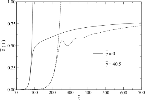
Figure 1: Volume average of $\bar{\phi}(\bar{t})$ as a function of dimensionless time $\bar{t}$ for the noncausal (solid) and causal (dashed) solutions. The two curves that exit the top of the plot are results from the linearized theory.

In Fig. 1 we present the time evolution of the volume average of the order parameter $\phi$, defined as $\bar{\phi}(t)=\frac{1}{N^{3}}\sum_{{\bf x}}\langle\bar{\phi}({\bf x},t)_{+}\rangle$, where $N^{3}$ is the total number of lattice points and the average is taken over different initial random configurations. $\phi({\bf x},t)_{+}$ indicates that only the positive values of the field are considered (i.e., a specific direction for the field has been selected). The rapid increase of $\bar{\phi}$ reflects the phenomenon of SD. The figure also shows the results by solving the linear equation. It shows that it performs extremely well up to and right after the spinodal growth of the order parameter, then justifying our previous analytical results based on the solution of the linear equation. The effect of $\gamma$ is seen to be more important at earlier times, consistent with the memory function used and becomes less important after the rapid growth of the order parameter (the spinodal explosion). It also shows the effect of a finite $\gamma$, increasing dramatically the delay of the spinodal explosion, as predicted by our previous analytical results. The time for reaching equilibrium is seen to be very long, as is common with the traditional noncausal CH equation. Also apparent from Fig. 1 are the oscillations in the order parameter for a finite $\gamma$, also predicted by our previous analysis. This is due to the increasing importance of the second-order time derivative as compared to the first-order one as $\gamma$ increases, i.e. as $\gamma$ increases the dissipation term becomes less important and the equation becomes more and more a wave-like equation. The estimated delay for the thermalization is even larger than the recent estimation FK for the time delay of the relaxation of a nonconserved order parameter.

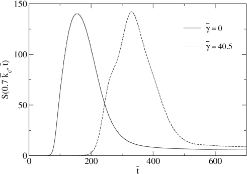
Figure 2: Spherically averaged structure function as a function of dimensionless time $\bar{t}$ for a $\bar{k}=0.7\bar{k}_{c}$ for the noncausal (solid) and causal (dashed) solutions.

We have also investigated the effect of memory for the structure function, $S(k,t)=|\phi({\bf k},t)|^{2}$. This quantity is important because it provides information on the space-time coarsening of the domains of the different phases. In Fig. 2 we present the results for the spherically averaged value of $S$ for $k=0.7k_{c}$ (to emphasize the fast growth of the long wavelength fluctuations with $k<k_{c}$). The spherical averaging for a given $k$ was done over momenta $k_{r}=\sqrt{k^{2}_{x}+k^{2}_{y}+k^{2}_{z}}$ such that $k-0.1\Delta\leq k_{r}\leq k+0.1\Delta$, with $\Delta=2\pi/L$, where $L$ is the size of the lattice. Consistently with Fig. 1, this figure shows the dramatic delay for the spinodal growth.

As conclusion, we have introduced memory into the CH equation. For a physical situation typical for the phenomenology of RHIC, we found that these ME can delay substantially the phase-separation process and consequently, there might not be enough time for the system to thermalize before the breakdown of the system due to expansion.

- (1) J.W. Cahn and J.C. Hilliard, J. Chem. Phys. 28 (1958) 258.
- (2) A.J. Bray, Adv. Phys. 43, 357 (1994); D. Gunton, M. San Miguel and P.S. Sahni, in Phase Transitions and Critical Phenomena, edited by C. Domb and J.L. Lebowitz (Academic Press, New York, 1983) Vol. 8, p. 267.
- (3) D. Jou, J. Casas-Vázquez and G. Lebon, Rep. Prog. Phys. 51 (1998) 1105; ibid. 62 (1999) 1035.
- (4) L. P. Kadanoff and P.C. Martin, Ann. Phys. (NY) 24 (1963) 419.
- (5) T. Koide, Phys. Rev. E 72 (2005) 026135.
- (6) J.W. Cahn, Acta Metall. 9 (1967) 795; Trans. Metall. Soc. AIME 242 (1968) 165.
- (7) M. Gleiser and R. O. Ramos, Phys. Rev. D 50 (1994) 2441; A. Berera and R. O. Ramos, Phys. Rev. D 63 (2001) 103509; Phys. Lett. B607, 1 (2005); Phys. Rev. D 71 (2005) 023513.
- (8) S. Gavin, Nucl. Phys. B351 (1991) 561; C. Greiner, K. Wagner and P. Rainhard, Phys. Rev. C 49 (1993) 1693; H. Heiselberg and X. N. Wang, Phys. Rev. C 53 (1996) 1892; S. Schmidt et al., Phys. Rev. D 59 (1999) 94005.
- (9) T. Koide and M. Maruyama, Nucl. Phys. A742 (2004) 95.
- (10) Y. Hama, T. Kodama and O. Socolowski Jr., Braz. J. Phys. 35 (2005) 24.
- (11) M.A. Aziz and S.Gavin, Phys. Rev. C 70 (2004) 034905.
- (12) D. Bower and S. Gavin, Phys. Rev. C 64 (2001) 051902.
- (13) J. Zhu, et al., Phys. Rev. E 60 (1999) 3564.
- (14) E.S. Fraga and G. Krein, Phys. Lett. B614 (2005) 181.