Chiral and U(1) axial symmetry restoration in linear sigma models with two quark flavors

Abstract

We study the restoration of chiral symmetry in linear sigma models with two quark flavors. The models taken into consideration have a $U(2)_{L}\times U(2)_{R}$ and an $O(4)$ internal symmetry. The physical mesons of these models are $\sigma$, pion, $\eta$ and $a_{0}$ where the latter two are not present in the $O(4)$ model. Including two-loop contributions through sunset graphs we calculate the temperature behavior of the order parameter and the masses for explicit chiral symmetry breaking and in the chiral limit. Decay threshold effects introduced by the sunset graphs alter the temperature dependence of the condensate and consequently that of the masses as well. This correctly reproduces a second-order phase transition for the $O(4)$ model and for the $U(2)_{L}\times U(2)_{R}$ model with an axial $U(1)$ anomaly as expected from universality class arguments. Chiral symmetry tends to be restored at higher temperatures in the two-loop approximation than in the Hartree–Fock approximation. To model a restoration of the axial $U(1)$ symmetry we imply a temperature-dependent anomaly parameter that sharply drops at about 175 MeV. This triggers the restoration of chiral symmetry before the full symmetry is restored and lowers the transition temperatures significantly below 200 MeV.

I Introduction

The Lagrangian of massless quantum chromodynamics (QCD) with $N_{f}$ quark flavors has a chiral $SU(N_{f})_{L}\times SU(N_{f})_{R}\times U(1)_{A}\times U(1)_{V}$ symmetry. A chiral quark condensate $\langle\bar{q}q\rangle\approx(300\,\mathrm{MeV})^{3}$ spontaneously breaks the $SU(N_{f})_{A}\times U(1)_{A}\simeq U(N_{f})_{A}$ part of the symmetry and generates $N_{f}^{2}$ Goldstone bosons. Apart from that there is also a violation of the $U(1)_{A}$ symmetry by instantons ’t Hooft (1976a, b); Pisarski and Wilczek (1984) giving mass to one of the Goldstone bosons. The $U(1)_{V}$ (vector) symmetry represents baryon number conservation, is always fulfilled and therefore will not be considered here. Adding mass terms like $m_{q}\,\bar{q}q$ to the QCD Lagrangian breaks the symmetry explicitly and gives all Goldstone bosons a mass, making them pseudo-Goldstone bosons.

At high temperatures chiral symmetry is expected to be restored. For finite quark masses this happens in a crossover transition such that the symmetry is (almost) restored when the temperature (to the third power) is of the order of the condensate $\langle\bar{q}q\rangle^{1/3}\approx 300\,\mathrm{MeV}$. Recently, lattice QCD has been able to determine the critical temperature of the chiral phase transition. For three flavors it has been found to be in the vicinity of 155 MeV while for two flavors it is about 170 MeV for a vanishing quark chemical potential Karsch (2002); Laermann and Philipsen (2003). In spite of being a challenging first-principle approach to QCD lattice calculation suffer from technical difficulties for small quark masses Fodor and Katz (2004) or for a chemical potential of the order of the temperature or larger de Forcrand and Philipsen (2002).

A different nonperturbative approach to QCD is the construction of low-energy effective theories of hadrons with the same chiral $U(N_{f})\times U(N_{f})$ symmetry. The color degrees of freedom are integrated out so that the low-energy behavior of QCD is governed by the lightest hadrons which are scalar and pseudoscalar mesons with, in general, light quark content. These particles can be found in linear sigma models Gell-Mann and Levy (1960). Since these models have the same symmetry as the underlying fundamental theory and thus belong to the same universality class they can be used to study the dynamics of phase transitions at finite temperature. Pisarski and Wilczek Pisarski and Wilczek (1984) found that there can be a second-order phase transition in presence of an explicitly broken $U(1)_{A}$ symmetry, whereas without this axial $U(1)$ anomaly the transition is of first order. The two-loop approximation investigated within this article will correctly reproduce these features in both the $U(2)_{L}\times U(2)_{R}$ and the $O(4)$ model.

Linear sigma models cannot be solved analytically so one has to make use of approximations. One problem arising at finite temperature is the breakdown of perturbation theory; at a temperature $T$, a (perturbative) expansion in powers of a coupling $g$ yields a new mass scale $gT$ that occurs in the denominators of loop graphs and cancels powers of the coupling constant in the perturbation expansion Dolan and Jackiw (1974); Braaten and Pisarski (1990a, b); Parwani (1992). So, terms of all orders of the coupling must be taken into account via resummation to avoid these unwanted cancellations. The resummation scheme we apply here is the so-called two-particle point-irreducible (2PPI) effective action introduced by Verschelde and Coppens Verschelde and Coppens (1992). Up to the level of the Hartree–Fock approximation it is identical to the two-particle irreducible (2PI) effective action formalism by Cornwall, Jackiw and Tomboulis Cornwall et al. (1974).

Linear sigma models with a $U(N_{f})\times U(N_{f})$ symmetry and two to four quark flavors have been studied in the Hartree–Fock or Hartree approximation within the last more than 25 years Röder et al. (2003); Lenaghan et al. (2000); Schaffner-Bielich (2000); Geddes (1980). The $O(N)$ model has received even greater attention; it has been analyzed using different resummation techniques, where various authors used local resummations Lenaghan and Rischke (2000); Dolan and Jackiw (1974); Baacke and Michalski (2003a); Petropoulos (1999); Patkós et al. (2002); Chiku and Hatsuda (1998); Nemoto et al. (2000); Smet et al. (2002); Verschelde and De Pessemier (2002), while, nowadays, nonlocal schemes, like the two-particle irreducible effective action Cornwall et al. (1974), have become popular as well Parwani (1992); de Godoy Caldas (2002); Röder et al. (2005); Röder (2005); Baacke and Michalski (2004a, b); Andersen et al. (2004). Furthermore, renormalization has become a heavily studied issue in this context van Hees and Knoll (2002a, b, c); Berges et al. (2005); Blaizot et al. (2004).

The Hartree–Fock approximation as well as the two-loop approximation of the 2PPI effective action violate Goldstone’s theorem because the formalism’s variational parameter associated to the Goldstone boson mass achieves finite values at temperatures above zero Baacke and Michalski (2003a); Verschelde and De Pessemier (2002); Nemoto et al. (2000). This problem can be overcome either by looking at the external (or physical) propagators Baacke and Michalski (2003a); van Hees and Knoll (2002c) — the derivatives of the one-particle irreducible (1PI) effective action — or by a construction described by Ivanov et al. Ivanov et al. (2005). For a renormalization group invariant approach to the $O(N)$ model see recent work of Destri and Sartirana Destri and Sartirana (2005a, b).

The $U(N_{f})_{L}\times U(N_{f})_{R}$ linear sigma model contains two $U(N_{f})$ isospin multiplets — a scalar and a pseudoscalar one — each of which is decomposed into an isosinglet and an $(N_{f}^{2}-1)$-dimensional isospin multiplet. For two flavors and unbroken isospin symmetry ($m_{u}=m_{d}$) we obtain four different mesons in the model, $\sigma$ [called $f_{0}(600)$ nowadays] with an isotriplet of (identical) $a_{0}$ bosons in the scalar sector, and $\eta$ with three pions in the pseudoscalar sector. The $O(N)$ linear sigma model only consists of a $\sigma$ meson and $N-1$ pions and is, for $N=N_{f}^{2}=4$, a limiting case of the $U(2)_{L}\times U(2)_{R}$ model for an infinitely strong $U(1)_{A}$ anomaly.

This article is organized as follows. In Secs. II and III we describe the $U(2)_{L}\times U(2)_{R}$ and the $O(N)$ linear sigma model and their pattern of symmetry breaking. Section IV deals with parameter fixing and numerical results in both models. Finally, in Sec. V we draw our conclusions and give an outlook. There is also an Appendix in which more details about the computation of the effective action of the $U(2)_{L}\times U(2)_{R}$ model are given.

II The $U(2)_{L}\times U(2)_{R}$ linear sigma model

II.1 Classical action

The Lagrangian of the $U(N_{f})_{R}\times U(N_{f})_{L}$ linear sigma model is given by

$$\begin{split}\mathscr{L}[\Phi]=\ &\mathrm{Tr}\;(\partial_{\mu}\Phi^{\dagger}\partial^{\mu}\Phi-m^{2}\Phi^{\dagger}\Phi)-\lambda_{1}[\mathrm{Tr}\;(\Phi^{\dagger}\Phi)]^{2}-\lambda_{2}\mathrm{Tr}\;[(\Phi^{\dagger}\Phi)^{2}]\\ &+c[\det\Phi+\det\Phi^{\dagger}]+\mathrm{Tr}\;[H(\Phi+\Phi^{\dagger})]\ .\end{split}$$ (1)

The field $\Phi$ is a complex $N_{f}\times N_{f}$ matrix containing the scalar and pseudoscalar mesons,

$$\Phi=T_{a}(\sigma_{a}+i\pi_{a}).$$ (2)

Here $\sigma_{a}$ are the scalar fields with $J^{P}=0^{+}$ while $\pi_{a}$ denotes the pseudoscalar ones with $J^{P}=0^{-}$. The last term in the Lagrangian (1) describes the interaction with an external field $H$ that breaks the symmetry explicitly,

$$H=T_{a}h_{a}\ .$$ (3)

$T_{a}$ are the generators of the group $U(N_{f})$ such that $\mathrm{Tr}\;(T_{a}T_{b})=\delta_{ab}/2$. The $U(N_{f})$ algebra is fulfilled

$$[T_{a},T_{b}] = if_{abc}\ T_{c}$$ (4a)

$$\{T_{a},T_{b}\} = d_{abc}\ T_{c}$$ (4b)

where $$f_{abc} d_{abc} U(N_{f}) a,b,c=0,\dots,N_{f}^{2}-1 SU(N_{f}) U(N_{f})$$ and are the antisymmetric and symmetric structure constants of and . They are identical to those of (with all indices starting from one), however for there is in addition

$$f_{ab0}=0\ ,\qquad d_{ab0}=\sqrt{\frac{2}{N_{f}}}\ \delta_{ab}\ .$$ (4c)

In the following we will deal only with the case $N_{f}=2$ which reduces the structure constants to

$$f_{ijk}=\varepsilon_{ijk}\quad\text{and}\quad d_{ijk}=0\quad\text{for}\quad i,j,k\in\{1,2,3\}\ ,$$ (5)

where $\varepsilon_{ijk}$ is the Levi–Civita symbol. The usual identification of the physical bosons for $N_{f}=2$ is (see, e.g., Ref. Röder et al. (2003))

$$\Phi=\frac{1}{\sqrt{2}}\left(\begin{array}[]{cc}\frac{1}{\sqrt{2}}\left(\sigma+a_{0}^{0}\right)&a_{0}^{+}\\ a_{0}^{-}&\frac{1}{\sqrt{2}}\left(\sigma-a_{0}^{0}\right)\end{array}\right)+\frac{i}{\sqrt{2}}\left(\begin{array}[]{cc}\frac{1}{\sqrt{2}}\left(\eta+\pi^{0}\right)&\pi^{+}\\ \pi^{-}&\frac{1}{\sqrt{2}}\left(\eta-\pi^{0}\right)\end{array}\right)\ .$$ (6)

Since isospin symmetry is left untouched the masses of all particles of one isovector are identical, i.e., $m_{a_{0}^{0}}=m_{a_{0}^{\pm}}$ and $m_{\pi^{0}}=m_{\pi^{\pm}}$.

II.2 Breaking the symmetry

The first three terms of the Lagrangian (1) are invariant under the group $U(2)_{L}\times U(2)_{R}\simeq SU(2)_{V}\times SU(2)_{A}\times U(1)_{A}\times U(1)_{V}$. The $U(1)_{V}$ vector symmetry reflects baryon number conservation of QCD. We will not deal with this symmetry in this paper as it is always conserved. Chiral symmetry is spontaneously broken if the vacuum expectation value of the field $\Phi$ does not vanish

$$\langle\Phi\rangle=T_{a}\phi_{a}\ .$$ (7)

The vacuum should be of even parity, so only $\phi_{a}=\langle\sigma_{a}\rangle$ is allowed. According to a theorem by Vafa and Witten Vafa and Witten (1984) global vector-like symmetries (isospin, baryon number) cannot be broken spontaneously. So, the remaining symmetry must be, at least, $SU(2)_{V}$. Spontaneously breaking $SU(2)_{A}\times U(1)_{A}$ yields four Goldstone bosons, $\eta$ and three pions. The determinants in the Lagrangian (1) break the $U(1)_{A}$ symmetry explicitly which represents the $U(1)$ axial anomaly ’t Hooft (1976a) whose strength is given here by the constant $c$. This anomaly makes the isosinglet Goldstone boson $\eta$ massive. The remaining $SU(2)$ symmetry (of three pions) stays intact if we assume the masses of the up and down quark to be equal so that only one diagonal generator gets a finite expectation value. So, we choose

$$\langle\Phi\rangle=T_{0}\phi_{0}=\frac{1}{2}\phi_{0}\ \openone\ .$$ (8)

Finally, the last term in the Lagrangian (1) explicitly breaks chiral symmetry and makes also the pions massive. It resembles the mass terms in the QCD Lagrangian where here $H$ corresponds to the quark mass matrix and $\Phi$ to the quark condensate. We will only deal with the case $h_{0}\neq 0$ and keep the $SU(2)$ isospin symmetry ($m_{u}=m_{d}$) conserved so that $h_{3}=0$.

With rising temperature we expect the chiral $SU(2)_{V}\times SU(2)_{A}\simeq SU(2)_{L}\times SU(2)_{R}$ symmetry to be restored so that the chiral partners ($\sigma$ and $\pi$, $\eta$ and $a_{0}$) become degenerate in mass. A violation of the axial $U(1)$ symmetry is inherent to the linear sigma model since its strength is directly given by the model’s parameter $c$. The restoration of this symmetry can only be modelled in a phenomenological way by making $c$ temperature-dependent, e.g., go down with rising $T$. For $c\to 0$ we expect the $\eta$ mass to become identical to the pion mass above a certain temperature so that there is a full $U(2)_{A}$ symmetry in the pseudoscalar sector. And, finally, all four masses are expected to become degenerate at temperatures above $\langle\bar{q}q\rangle^{1/3}\approx 300$ MeV for explicit symmetry breaking or above a critical temperature $T_{c}$ in the chiral limit.

II.3 Effective action

We compute the effective action using the 2PPI formalism Smet et al. (2002); Verschelde and De Pessemier (2002); Verschelde and Coppens (1992); Baacke and Michalski (2003a) and include all graphs up to two loops. The reader is referred to the Appendix for details of the computation. Here, we will only give the final result for the effective potential:

$$V_{\mathrm{eff}}({M}^{2},\phi_{0})=V_{\mathrm{cl}}(\phi_{0})+V_{\mathrm{db}}({M}^{2},\phi_{0})+V_{q}({M}^{2},\phi_{0})\ .$$ (9)

It is a function of the masses ${M}_{\sigma}^{2}$, ${M}_{\pi}^{2}$, ${M}_{\eta}^{2}$ and ${M}_{a_{0}}^{2}$ (denoted by ${M}^{2}$ for brevity) and the condensate $\phi_{0}$. The classical part is

$$V_{\mathrm{cl}}(\phi_{0})=\frac{1}{2}(m^{2}-c)\phi_{0}^{2}+\left(\frac{\lambda_{1}}{4}+\frac{\lambda_{2}}{8}\right)\phi_{0}^{4}-h_{0}\,\phi_{0}\ .$$ (10)

The quantum part $V_{q}$ contains all two-particle point-irreducible (2PPI) graphs that can be made of the vertices of the shifted Lagrangian except for the double bubbles which will be taken care of by $V_{\mathrm{db}}$. The propagators within these graphs are defined by an effective mass and have the Euclidean form

$$G_{*}(p)=\frac{1}{p^{2}+{M}_{*}^{2}}\ .$$

Here, we only take into account 2PPI graphs with one and two loops which leads to

$$\begin{split}V_{q}(M^{2},\phi_{0})=\ &\frac{1}{2}\ln\det(\partial^{2}+{M}_{\sigma}^{2})+\frac{1}{2}\ln\det(\partial^{2}+{M}_{\eta}^{2})\\ &+\frac{3}{2}\ln\det(\partial^{2}+{M}_{a_{0}}^{2})+\frac{3}{2}\ln\det(\partial^{2}+{M}_{\pi}^{2})\\ &+V_{\mathrm{sunsets}}(M^{2},\phi_{0})\end{split}$$ (11)

The sunset contribution is given by (note the minus sign)

$$\begin{split}V_{\mathrm{sunsets}}(M^{2},\phi_{0})=-\phi_{0}^{2}\,\Biggl{[}&\left(\lambda_{1}+\frac{3}{2}\lambda_{2}\right)^{2}(3\,S_{\sigma\sigma\sigma}+3\,S_{\sigma a_{0}a_{0}}+S_{\sigma\eta\eta})\\ &+\left(\lambda_{1}+\frac{\lambda_{2}}{2}\right)^{2}S_{\sigma\pi\pi}+\frac{3}{2}\lambda_{2}^{2}\,S_{a_{0}\eta\pi}\Biggr{]}\ ,\end{split}$$ (12)

where $S_{ijk}$ denotes a sunset graph made of the propagators of the particles $i$, $j$ and $k$. A graphical representation of these contributions can be found in Fig. 1. These graphs arise from the possible decays of $\sigma\to\pi\pi$, $\sigma\to\eta\eta$ and $a_{0}\to\eta\pi$.

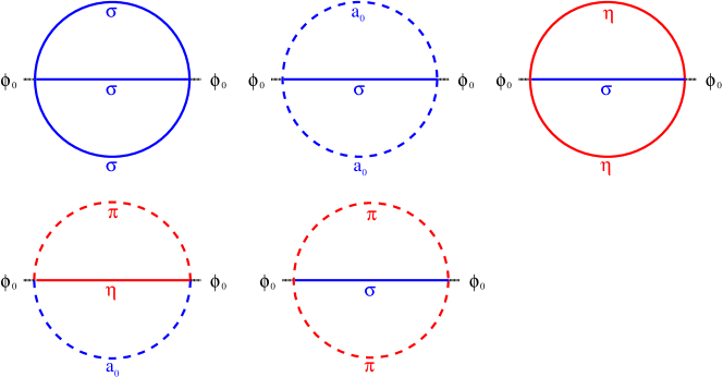
Figure 1: The sunset graphs as in Eq. (12). Scalars are drawn in blue, pseudoscalars in red. Dashed lines represent isotriplets while solid lines are used for isosinglets.

$V_{\mathrm{db}}$ is the double-bubble part that receives a special treatment in the 2PPI formalism

$$\begin{split}V_{\mathrm{db}}({M}^{2},\phi_{0})=\ &-\left(\frac{\lambda_{1}}{4}+\frac{\lambda_{2}}{8}\right)(3\,\Delta_{\sigma}^{2}+15\,\Delta_{\pi}^{2}+6\,\Delta_{\sigma}\Delta_{\pi})\\ &-\left(\frac{\lambda_{1}}{4}+\frac{\lambda_{2}}{8}\right)(3\,\Delta_{\eta}^{2}+15\,\Delta_{a_{0}}^{2}+6\,\Delta_{\eta}\Delta_{a_{0}})\\ &-\left(\frac{\lambda_{1}}{2}+\frac{\lambda_{2}}{4}\right)\Delta_{\sigma}\Delta_{\eta}-3\,\left(\frac{\lambda_{1}}{2}+\frac{3}{4}\lambda_{2}\right)\Delta_{a_{0}}\Delta_{\sigma}\\ &-3\,\left(\frac{\lambda_{1}}{2}+\frac{3}{4}\lambda_{2}\right)\Delta_{\pi}\Delta_{\eta}-3\,\left(\frac{3}{2}\lambda_{1}+\frac{7}{4}\lambda_{2}\right)\Delta_{a_{0}}\Delta_{\pi}\ .\end{split}$$ (13)

All quantities $\Delta$ are obtained via

$$\Delta_{*}({M}^{2},\phi_{0})=2\,\frac{\partial}{\partial{M}^{2}_{*}}V_{q}({M}^{2},\phi_{0})$$ (14)

where $*$ stands for $\sigma$, $a_{0}$, $\eta$ or $\pi$ and $M^{2}$ is a short-hand notation for all four masses. So, these quantities are explicit function of the mass matrix ${M}^{2}$ and the condensate $\phi_{0}$.

II.4 Equations of motion

The mass gap equations in the 2PPI effective action formalism are given by

$$\frac{\partial V_{\mathrm{eff}}}{\partial M^{2}_{*}}=0\qquad\text{with}\quad*=\sigma,a_{0},\eta,\pi$$

and read explicitly

$$\begin{split}{M}^{2}_{\sigma}=&m^{2}-c+3\left(\lambda_{1}+\frac{\lambda_{2}}{2}\right)\phi_{0}^{2}+3\,\left(\lambda_{1}+\frac{\lambda}{2}\right)(\Delta_{\sigma}+\Delta_{\pi})\\ &+3\,\left(\lambda_{1}+\frac{3}{2}\lambda_{2}\right)\Delta_{a_{0}}+\left(\lambda_{1}+\frac{\lambda_{2}}{2}\right)\,\Delta_{\eta}\end{split}$$ (15a)

$$\begin{split}{M}^{2}_{\pi}=&m^{2}-c+\left(\lambda_{1}+\frac{\lambda_{2}}{2}\right)\phi_{0}^{2}+\left(\lambda_{1}+\frac{\lambda}{2}\right)(\Delta_{\sigma}+5\,\Delta_{\pi})\\ &+\left(\lambda_{1}+\frac{3}{2}\lambda_{2}\right)\Delta_{\eta}+\left(3\,\lambda_{1}+\frac{7}{2}\lambda_{2}\right)\,\Delta_{a_{0}}\end{split}$$ (15b)

$$\begin{split}{M}^{2}_{\eta}=&m^{2}+c+\left(\lambda_{1}+\frac{\lambda_{2}}{2}\right)\phi_{0}^{2}+\left(\lambda_{1}+\frac{\lambda}{2}\right)3\,(\Delta_{\eta}+\Delta_{a_{0}})\\ &+\left(\lambda_{1}+\frac{\lambda_{2}}{2}\right)\Delta_{\sigma}+3\,\left(\lambda_{1}+\frac{3}{2}\lambda_{2}\right)\,\Delta_{\pi}\end{split}$$ (15c)

$$\begin{split}{M}^{2}_{a_{0}}=&m^{2}+c+\left(\lambda_{1}+\frac{3}{2}\lambda_{2}\right)\phi_{0}^{2}+\left(\lambda_{1}+\frac{\lambda}{2}\right)(\Delta_{\eta}+5\,\Delta_{a_{0}})\\ &+\left(\lambda_{1}+\frac{3}{2}\lambda_{2}\right)\Delta_{\sigma}+\left(3\,\lambda_{1}+\frac{7}{2}\lambda_{2}\right)\,\Delta_{\pi}\ .\end{split}$$ (15d)

The formalism is made such that these equations resemble those of the Hartree–Fock approximation with the decisive difference that here $\Delta_{*}$ is not a single bubble but calculated from Eq. (14). Neglecting the sunsets contributions to $V_{q}$ in Eq. (14) would reduce all quantum corrections to simple bubbles; in this way the Hartree–Fock approximation is regained. Solving Eqs. (15) for all four quantum corrections one finds a (quite lengthy) expression for each quantum correction in terms of all four masses and the condensate. The equation of motion for the condensate

$$\frac{\partial}{\partial\phi_{0}}V_{\mathrm{eff}}({M}^{2},\phi_{0})=0$$

can be put in a very easy form by simplifying $V_{\mathrm{db}}({M}^{2},\phi_{0})+V_{\mathrm{cl}}(\phi_{0})$:

$$h_{0}={M}^{2}_{\sigma}\,\phi_{0}-(2\lambda_{1}+\lambda_{2})\,\phi_{0}^{3}+\frac{\partial}{\partial\phi_{0}}V_{\mathrm{sunsets}}\ .$$ (16)

Neglecting the sunsets this equation is equivalent to the one found in the Hartree–Fock approximation Röder et al. (2003).

III The $O(N)$ linear sigma model

III.1 Langrangian

The linear sigma model with an $O(4)$ symmetry is obtained from the $U(2)_{V}\times U(2)_{A}$ model in the limit of infinite anomaly $c\to\infty$ with fixed $(m^{2}-c)\to m^{2}_{O(4)}$. The masses of both the $\eta$ and the $a_{0}$ mesons become infinite and thus these two mesons drop out of the spectrum. The coupling is renamed to $\lambda\equiv\left(\lambda_{1}+\frac{\lambda_{2}}{2}\right)$, and $\sigma$ and the three pions now share one $O(4)$ multiplet. Extending the isospin symmetry from four to $N$ dimensions we can now write down the well-known Lagrangian of the $O(N)$ linear sigma model

$$\mathscr{L}[\Phi]=\frac{1}{2}\left(\partial_{\mu}\Phi_{i}\right)^{2}-\frac{1}{2}m^{2}\Phi_{i}^{2}-\frac{\lambda}{4}\left(\Phi_{i}^{2}\right)^{2}+h_{i}\,\Phi_{i}\quad\text{with}\quad i=1,\dots,N$$ (17)

which has been studied extensively Lenaghan and Rischke (2000); Baacke and Michalski (2003a, b); Petropoulos (1999); Dolan and Jackiw (1974); Chiku and Hatsuda (1998); Nemoto et al. (2000); Smet et al. (2002); Verschelde and De Pessemier (2002); Andersen et al. (2004). In this article we will extend the analysis performed earlier Baacke and Michalski (2003a, b) to the case of explicit symmetry breaking and realistic values of the parameters.

III.2 Equations of motion

The equations of motion are obtained from the 2PPI effective potential where the vacuum expectation value is set to be

$$\langle\Phi_{i}\rangle=\phi_{0}\,\delta_{0i}\ ,$$

so that the 2PPI effective action reads Baacke and Michalski (2003a); Verschelde and De Pessemier (2002)

$$\begin{split}V_{\mathrm{eff}}(\phi_{0};M_{\sigma}^{2},M_{\pi}^{2})=\ &\frac{1}{2}M_{\sigma}^{2}\phi_{0}^{2}-\frac{\lambda}{2}\phi_{0}^{4}-h_{0}\,\phi_{0}+\frac{m^{2}}{2\lambda\,(N+2)}\left[M_{\sigma}^{2}+(N-1)M_{\pi}^{2}\right]\\ &-\frac{1}{8\lambda\,(N+2)}\biggl{[}(N+1)\,M_{\sigma}^{4}+3\,(N-1)M_{\pi}^{4}\\ &-2\,(N-1)\,M_{\sigma}^{2}M_{\pi}^{2}+2N\lambda^{2}m^{4}\biggr{]}+V_{q}(\phi_{0};M_{\sigma}^{2},M_{\pi}^{2})\ .\end{split}$$ (18)

The quantum corrections consist of the following one- and two-loop terms

$$\begin{split}V_{q}(\phi_{0};M_{\sigma}^{2},M_{\pi}^{2})=\ &\frac{1}{2}\ln\det(\partial^{2}+{M}_{\sigma}^{2})+\frac{N-1}{2}\ln\det(\partial^{2}+{M}_{\pi}^{2})\\ &-\lambda^{2}\phi_{0}^{2}\left[3\,S_{\sigma\sigma\sigma}+(N-1)\,S_{\sigma\pi\pi}\right]\ .\end{split}$$ (19)

The mass gap equations follow from the stationarity conditions

$$\frac{\partial}{\partial M_{\sigma}}V_{\mathrm{eff}}=0\quad\text{and}\quad\frac{\partial}{\partial M_{\pi}}V_{\mathrm{eff}}=0\ .$$

They read

$${M}_{\sigma}^{2} = m^{2}+3\,\lambda\phi_{0}^{2}+\lambda\left[3\,\Delta_{\sigma}+(N-1)\,\Delta_{\pi}\right]$$ (20a)

$${M}_{\pi}^{2} = m^{2}+\lambda\phi_{0}^{2}+\lambda\left[\Delta_{\sigma}+(N+1)\,\Delta_{\pi}\right]\ ,$$ (20b)

where all quantum corrections $\Delta$ are explicit functions of both the condensate $\phi_{0}$ and the masses defined as

$$\Delta_{i}({M}_{\sigma},{M}_{\pi};\phi_{0})=2\,\frac{\partial V_{q}}{\partial{M}_{i}^{2}}\ .$$

The equation for the condensate has the same structure as the one in the $U(2)_{L}\times U(2)_{R}$ model, Eq. (16),

$$h_{0}=\left\{{M}_{\sigma}^{2}-2\lambda\,\phi_{0}^{2}-2\,\lambda^{2}\left[3\,S_{\sigma\sigma\sigma}+(N-1)\,S_{\sigma\pi\pi}\right]\right\}\,\phi_{0}\ .$$ (21)

In the following we will only investigate the case $N=4$.

IV Numerical Results

IV.1 Parameter fixing and loop graphs at finite temperature

The parameters in both models are fixed such that at $T=0$ the values of all masses are equal to the values in the Particle Physics Booklet Eidelman et al. (2004), cf. Table 1, where we choose the mass of the $\sigma$ meson to be 600 MeV. The value of the condensate $\phi_{0}$ is related to the mesons decay constants $f_{a}$ and determined by the PCAC (partial conservation of axial vector current) hypothesis

$$f_{a}=d_{aa0}\ \phi_{0}\equiv\phi_{0}\ .$$

This fixes the condensate to $\phi_{0}=f_{\pi}$ because $d_{aa0}=1$, so all decay constants are the same.

For the two models of this paper the fixing can be done in a unique way because there are as many equations of motion as parameters. At tree-level it could be done even in the chiral limit (with $h_{0}$ fixed to zero) since the equation for the condensate coincides with the one for the pion mass. Problems occur if one wants to include terms that contain a renormalization scale because, first, in the chiral limit there is only one possible value for this scale where the parameters can be fixed and, second, for explicit symmetry breaking the temperature-dependence of the condensate and the masses is varying with the renormalization scale Lenaghan and Rischke (2000). So, the system only gets an extra parameter and all quantities are logarithmically dependent on this scale which makes the results somewhat arbitrary. Furthermore, terms originating from renormalization can be such that the gap equations are not solvable above a certain temperature Baym and Grinstein (1977); Chiku and Hatsuda (1998); Bardeen and Moshe (1986). Lenaghan and Rischke Lenaghan and Rischke (2000) have also shown that, in the $O(N)$ model, there is no qualitative difference whether one includes the finite renormalization terms or not. In order to get rid of this extra parameter we take the phenomenological approach proposed before Röder et al. (2003); Lenaghan and Rischke (2000); Lenaghan et al. (2000) and set all finite terms arising from regularization equal to zero which makes all quantum corrections only play a role at finite temperature. So, effectively the parameters are fixed at tree-level. The resulting values can be found in Tables 2 and 3.

Neglecting finite terms from renormalization the one-loop graphs at finite temperature — the boson determinants in the effective action and the single bubble (or tadpole) $\mathcal{B}$ — are given by the following equations Baacke and Michalski (2003a)

$$\ln\det(\partial^{2}+M_{i}^{2}) = \frac{T}{\pi^{2}}\int_{0}^{\infty}\!\!\!dp\ {\bf p}^{2}\,\ln\left[1-e^{-E({\bf p})/T}\right]$$ (22a)

$$\mathcal{B}_{i} = \frac{\partial}{\partial M_{i}^{2}}\ln\det(\partial^{2}+M_{i}^{2})=\frac{1}{2\,\pi^{2}}\int_{0}^{\infty}\!\!\!dp\ \frac{{\bf p}^{2}}{E_{i}(\bf p)}\,n_{i}({\bf p})\ ,$$ (22b)

where $E_{i}({\bf p})=\sqrt{{\bf p}^{2}+M_{i}^{2}}$ and $n_{i}$ is the Bose-Einstein distribution

$$n_{i}({\bf p})=\frac{1}{e^{E_{i}({\bf p})/T}-1}\ .$$ (23)

The sunset graph with three different masses $M_{i}$, $M_{j}$ and $M_{k}$ is composed of three parts in each of which two of the three particles are taken from the heat bath

$$S_{ijk}=\mathcal{S}^{(2)}_{(ij)k}+\mathcal{S}^{(2)}_{(ki)j}+\mathcal{S}^{(2)}_{(jk)i}\ .$$ (24)

Here, $\mathcal{S}^{(2)}_{(ij)k}$ is a sunset graph with $i$ and $j$ being thermal lines Baacke and Michalski (2003a)

$$\mathcal{S}^{(2)}_{(ij)k}=\frac{1}{32\,\pi^{4}}\iint_{0}^{\infty}\!\!\!dp_{i}\,dp_{j}\ \frac{p_{i}p_{j}}{E_{i}E_{j}}\,n_{i}({\bf p}_{i})\,n_{i}({\bf p}_{i})\,\ln\left|\frac{Y_{(ij)k}^{+}}{Y_{(ij)k}^{-}}\right|$$ (25)

with

$$Y_{(ij)k}^{\pm}=\left[(E_{i}+E_{j})^{2}-(E_{(ij)k}^{\pm})^{2}\right]\cdot\left[(E_{i}-E_{j})^{2}-(E_{(ij)k}^{\pm})^{2}\right]$$

and

$$E_{(ij)k}^{\pm}=\sqrt{(p_{i}\pm p_{j})^{2}+M_{k}^{2}}\ .$$

	mass in MeV
	explicit symmetry breaking		chiral limit
particle	with anomaly	without anomaly	with anomaly	without anomaly
$\sigma$	600.0	600.0	600.0	600.0
$\pi$	139.6	139.6	0	0
${a_{0}}$	984.7	984.7	984.7	984.7
$\eta$	547.3	139.6	547.3	0

Table 1: Meson masses in the linear sigma models with and without axial anomaly for explicit symmetry breaking and in the chiral limit. Note that, of course, there is no $a_{0}$ and $\eta$ meson in the $O(4)$ model.

	explicit symmetry breaking		chiral limit
parameter	with anomaly	without anomaly	with anomaly	without anomaly
$m^{2}$	$-(103.78$ MeV)2	$-(388.34$ MeV)2	$-(173.87)$ MeV)2	$-(424.26$ MeV)2
$c$	(374.22 MeV)2	0	(387.00 MeV)2	0
$h_{0}$	(121.60 MeV)3	(121.60 MeV)3	0	0
$\lambda_{1}$	$-19.30$	$-35.70$	$-19.14$	$-37.63$
$\lambda_{2}$	78.49	111.29	82.73	119.71
$\phi_{0}$	92.4 MeV	92.4 MeV	90 MeV	90 MeV

Table 2: Parameters in the $U(2)_{L}\times U(2)_{R}$ model for masses as in Table 1.

parameter	explicit symmetry breaking	chiral limit
$m^{2}$	$-(388.34$ MeV)2	$-(424.26$ MeV)2
$h_{0}$	(121.6 MeV)3	0
$\lambda$	$19.94$	$22.22$
$\phi_{0}$	92.4 MeV	90 MeV

Table 3: Parameters in the $O(4)$ model for masses as in Table 1.

IV.2 $O(4)$ model

For a given temperature $T$ we let $N=4$, fix the value of $\phi_{0}$ and then numerically extremize the effective potential in Eq. (18) with respect to $M_{\sigma}$ and $M_{\pi}$. Thereby, we obtain a 1PI potential that is only a function of $\phi_{0}$. Using the equation of motion for the condensate (21) we eventually find the temperature-dependent value of the order parameter $f_{\pi}(T)$. This quantity is plotted in Fig. 2. For comparison we also plot the result for the Hartree–Fock approximation and for a simplified two-loop approximation (HF in 2-loop) which consists in solving the gap equations (20) in the Hartree–Fock approximation but the condensate equation (21) with the sunset contributions. In the chiral limit the transition temperature is almost the same as in the true two-loop approximation though the condensate drops faster at lower temperatures and then eventually approaches zero at $T\approx 210$ MeV. In the chiral limit of the Hartree–Fock approximation, there is a first-order phase transition at $T_{c}\approx 181$ MeV whereas the two-loop approximations (both the true and the simplified one) correctly reproduce a second-order transition though at a higher temperature of about 210 MeV.

For explicit symmetry breaking the simplified two-loop approximation results lie on top of the Hartree–Fock results, only the true two-loop approximation yields slight deviations. There, the condensate drops faster at temperatures below 200 MeV and decreases more slowly for temperatures above 250 MeV than but in all approximations the crossover temperature — the one where the slope of $f_{\pi}(T)$ is largest — is about 225 MeV.

The temperature dependence of the $\sigma$ and pion mass is displayed in Fig. 3. In the chiral limit [Fig. 3(a)] the $\sigma$ mass behaves similarly in both approximations while the pion mass first increases before it slightly drops at $T\approx 195$ MeV (180 MeV in the chiral limit). Beyond temperatures of about 200 MeV the pion mass in both approximations is almost the same. In the vicinity of 300 MeV both masses become identical, a sign for the restoration of chiral symmetry. There, the temperature (to the third power) is equal to the value of the chiral quark condensate (see above). In the chiral limit [Fig. 3(b)] the pion mass first grows stronger in the two-loop approximation than in Hartree–Fock, then it slightly drops before the critical temperature is reached and the masses become the same.

Moreover, there is a violation of Goldstone’s theorem at finite temperature in the chiral limit because even for temperatures lower than the critical one, $M_{\pi}$ is not equal to zero although the symmetry is spontaneously broken. This phenomenon can also be found in earlier results on the $O(N)$ model Baacke and Michalski (2003a); Verschelde and De Pessemier (2002); Nemoto et al. (2000); Röder et al. (2003). We will comment on this in Sec. V.

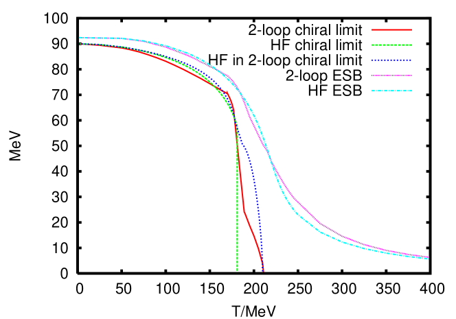
Figure 2: Temperature dependence of the condensate in the $O(4)$ model. Comparison of the two-loop approximation with the Hartree–Fock approximation (HF).

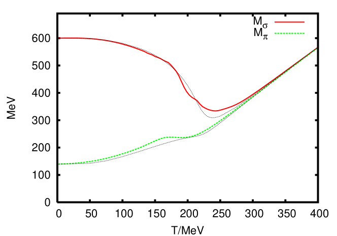
(a) Explicit symmetry breaking.

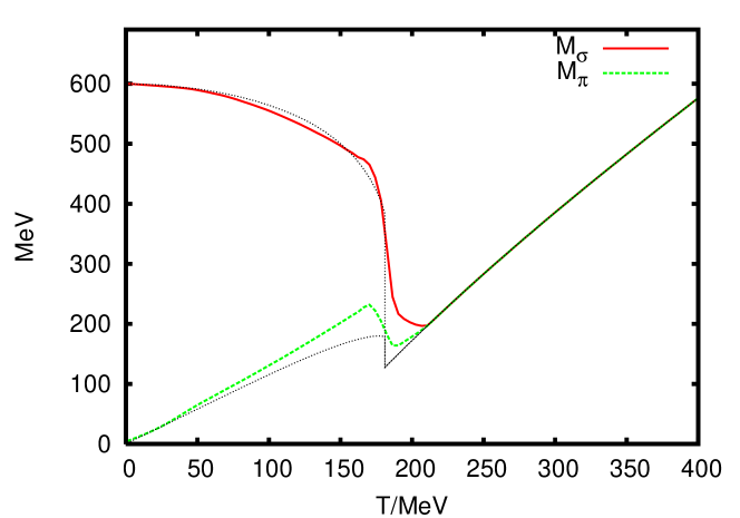
(b) Chiral limit.

Figure 3: Temperature dependence of the masses in the $O(4)$ model. Comparison of the two-loop approximation with Hartree–Fock (dotted).

IV.3 $U(2)_{L}\times U(2)_{R}$ model

The procedure performed for the $O(N)$ model, cf. Sec. IV.2, cannot be done for the $U(2)_{L}\times U(2)_{R}$ model because it turns out that the potential $V=V_{\mathrm{cl}}+V_{\mathrm{db}}$ has only a saddle point with respect to the four masses instead of a local extremum.

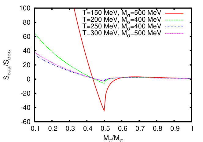
Figure 4: The ratio $S_{\sigma\pi\pi}/S_{\sigma\sigma\sigma}$ for $M_{\sigma}=500$ MeV at $T=150$ MeV and $T=300$ MeV, and $M_{\sigma}=400$ MeV at $T=200$ MeV and $T=250$ MeV.

Solving the gap equations (15) is a cumbersome procedure because they contain derivatives of the sunset graph with respect to a mass. And in the vicinity of the decay threshold of the particles involved in a sunset graph, e.g. $M_{\sigma}\simeq 2\,M_{\pi}$, the sign of the derivative of the sunset graph quickly changes (see Fig. 4) which results in a numerically unstable behavior in this region. To avoid this trouble a simplified approximation is used (cf. Sec. IV.2): we solve the mass gap equations (15) in the Hartree–Fock approximation, i.e., the quantum corrections $\Delta$ to the masses only consist of single bubbles given by Eq. (22b). We substitute these masses into the two-loop equation for the condensate (16) to obtain the temperature-dependent order parameter or decay constant $f_{\pi}(T)$ and, for simplicity, call this approximation “two-loop” from now on.

IV.3.1 Model with axial $U(1)$ anomaly

In Fig. 5 we show the temperature dependence of the condensate in the $U(2)_{L}\times U(2)_{R}$ model with an axial anomaly. In the chiral limit of the Hartree–Fock approximation there is a first-order phase transition at $T_{c}\approx 178$ MeV where the condensate discontinuously drops down from about 52 MeV to zero. In the two-loop approximation we find a second-order transition at $T_{c}\approx 272$ MeV. So, the two-loop approximation correctly reproduces the order of the phase transition obtained from universality class arguments Pisarski and Wilczek (1984), though the critical temperature is about 100 MeV higher than suggested by QCD lattice calculations Karsch (2002); Laermann and Philipsen (2003). The artificial first-order transition in the Hartree–Fock approximation has been discovered before by Röder et al. for a $\sigma$ mass of 400 MeV Röder et al. (2003). For both explicit symmetry breaking and in the chiral limit the order parameter decreases more slowly with rising temperature in the two-loop approximation than in the Hartree–Fock approximation and exhibits some “bumps” in the curve. The reason for that behavior is a decay threshold effect caused by the sunset graphs [cf. Eq. (12) and Fig. 4]. To check where the thresholds are crossed we plot the mass ratios for the decays $\sigma\to\pi\pi$, $a_{0}\to\eta\pi$ and $\sigma\to\eta\eta$ in Fig. 6.

The curve of the order parameter in the two-loop approximation deviates from the one of the Hartree–Fock approximation at a temperature of about 175-180 MeV. This is the region where the thresholds of the decays $\sigma\to\pi\pi$ and $a_{0}\to\eta\pi$ are crossed (see Fig. 6). The sunsets become larger with rising temperature but also decrease with masses approaching the threshold from below. The latter behavior suddenly changes at the threshold and the sunsets suddenly grow which causes the immediate deviation from the Hartree–Fock results. Looking at the equation for the condensate (16) one can roughly conclude that a larger value of the condensate is needed to compensate for the contribution from the sunset terms .

Comparing the prefactors of the different sunsets in Eq. (12) using the numerical values of the couplings from Table 2 we notice that, in the case of a finite $U(1)_{A}$ anomaly, the contributions from $S_{\sigma\eta\eta}$ and $S_{a_{0}\eta\pi}$ are almost of the same size whereas $S_{\sigma\pi\pi}$ is smaller by a factor of eight. Furthermore, the sunset term has dimension two and thus scales with temperature and the masses of the particles within. So, considering the prefactors and the different values for the masses — where $M_{a_{0}}$ and $M_{\eta}$ are the two largest ones — the deviation from the Hartree–Fock approximation is dominated by a threshold effect of the decay $a_{0}\to\eta\pi$.

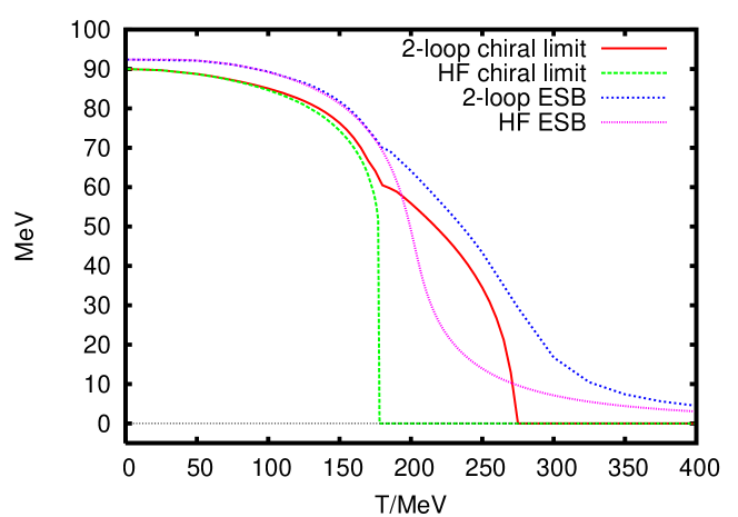
Figure 5: Temperature dependence of the condensate in the $U(2)_{L}\times U(2)_{R}$ model with an axial $U(1)$ anomaly. Comparison of the two-loop approximation with Hartree–Fock (HF) for explicit symmetry breaking (ESB) and in the chiral limit.

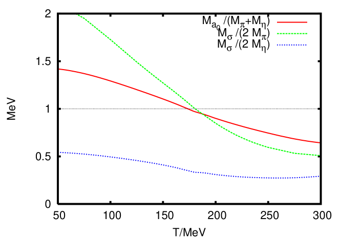
(a) Explicit symmetry breaking.

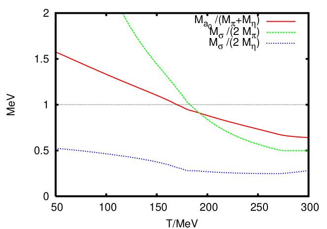
(b) Chiral limit.

Figure 6: Thresholds for the decays $\sigma\to\pi\pi$, $a_{0}\to\eta\pi$ and $\sigma\to\eta\eta$ in the $U(2)_{L}\times U(2)_{R}$ model with axial anomaly as.

The temperature-dependent masses for the $U(2)_{L}\times U(2)_{R}$ model are displayed in Fig. 7. Especially the masses of the scalar mesons $\sigma$ and $a_{0}$ behave differently in the two-loop approximation than in Hartree–Fock whereas the masses of both pseudoscalar mesons exhibit no qualitative difference in their temperature dependence between the two approximations. The observed deviations are due to the aforementioned threshold effects through sunset graphs. At a temperature of about 300 MeV (or beyond $T_{c}\approx 272$ MeV in the chiral limit) the masses of the chiral partners become identical so that chiral symmetry is restored. The $U(1)_{A}$ symmetry remains broken since the parameter $c$ is not a function of temperature. The gap between the mass squares of the isospin partners $\eta$ and $\pi$ (or $\sigma$ and $a_{0}$) remains equal to $2c$ according to Eq. (15). In the $U(2)_{L}\times U(2)_{R}$ model as well, the pion mass is finite in the chiral limit even for $T<T_{c}$ which was discovered in the Hartree–Fock approximation earlier Röder et al. (2003). We will give a statement concerning a possible violation of Goldstone’s theorem in Sec. V.

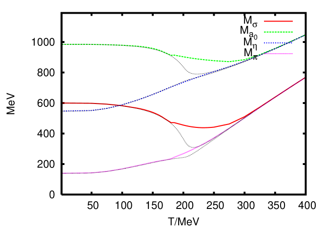
(a) Explicit symmetry breaking

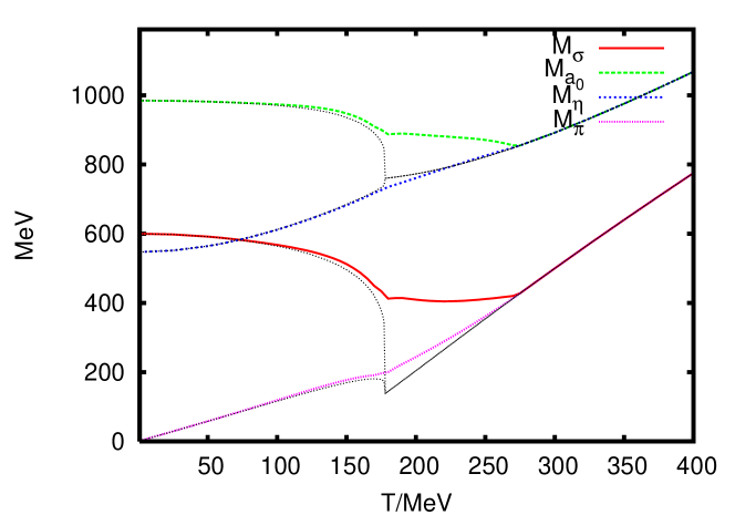
(b) Chiral limit.

Figure 7: Masses in the $U(2)_{L}\times U(2)_{R}$ model with axial anomaly as functions of temperature. Comparison of the two-loop approximation with Hartree–Fock (dotted lines).

IV.3.2 Model without axial $U(1)$ anomaly

For the $U(2)_{L}\times U(2)_{R}$ model without axial $U(1)$ anomaly we plot the condensate vs. temperature in Fig. 8. In the chiral limit there is a first-order phase transition at $T_{c}\approx 200$ MeV ($T_{c}\approx 170$ MeV in Hartree–Fock) which is expected from the respective universality class Pisarski and Wilczek (1984).

Here, the deviation from the Hartree–Fock approximation sets in at lower temperatures because the $\sigma\to\eta\eta$ threshold is crossed already at temperatures about 100 MeV, followed by $\sigma\to\pi\pi$ at about 175 MeV and, finally, the on-shell decay $a_{0}\to\eta\pi$ becomes impossible at 200 MeV (see Fig. 9). Compared to the case with a finite axial anomaly the effect of the sunset $S_{\sigma\pi\pi}$ is only about 7% (instead of 12%) of that of the other two. So, in this case as well, the deviation from the Hartree–Fock approximation is dominated by $S_{a_{0}\eta\pi}$.

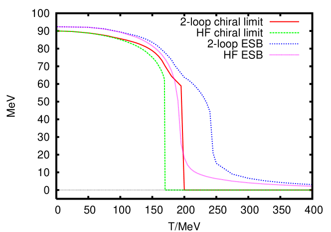
Figure 8: Temperature dependence of the condensate in the $U(2)_{L}\times U(2)_{R}$ model without an axial anomaly. Comparison of the two-loop approximation with Hartree–Fock (HF) for explicit symmetry breaking (ESB) and in the chiral limit.

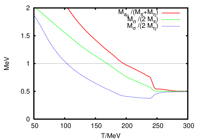
(a) Explicit symmetry breaking.

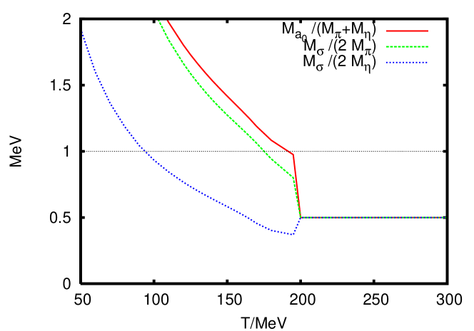
(b) Chiral limit.

Figure 9: Thresholds for the decays $\sigma\to\pi\pi$, $a_{0}\to\eta\pi$ and $\sigma\to\eta\eta$ in the $U(2)_{L}\times U(2)_{R}$ model without axial anomaly.

In Fig. 10(a) we observe that, for explicit symmetry breaking, the masses of the chiral partners tend to become identical at 250 MeV (200 MeV in Hartree–Fock) before the actual restoration of the full $U(2)_{L}\times U(2)_{R}$ symmetry takes place at about 300 MeV. In the chiral limit, [Fig. 10(b)] these two points coincide when the critical temperature is reached. At finite temperature the mass of the $\eta$ meson differs from the pion mass although they both started from 139.6 MeV (or zero in the chiral limit) at zero temperature. This indicates that the approximations considered in this article are not well-suited to model the $\eta$ meson as a fourth (pseudo-)Goldstone boson since they seem to contain an effective $U(1)_{A}$ breaking through the unequal treatment of $\eta$ and $\pi$ in the gap equations (15). This has been found before in the Hartree–Fock approximation Röder et al. (2003). In the case of a vanishing $U(1)$ anomaly as well, Goldstone’s theorem seems to be violated in the chiral limit as mentioned before because $M_{\eta}$ and $M_{\pi}$ are finite below $T_{c}$.

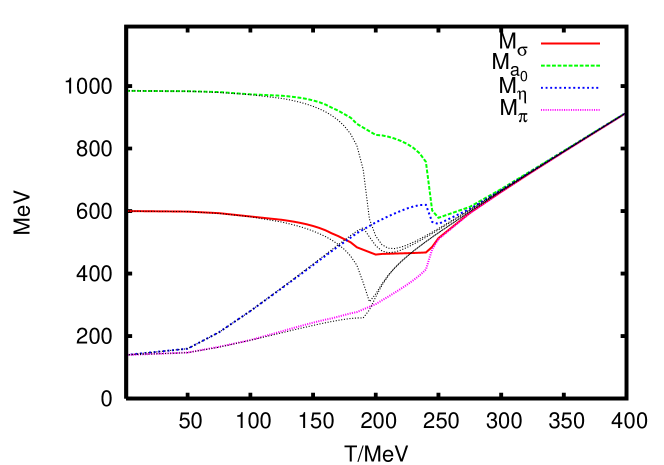
(a) Explicit symmetry breaking

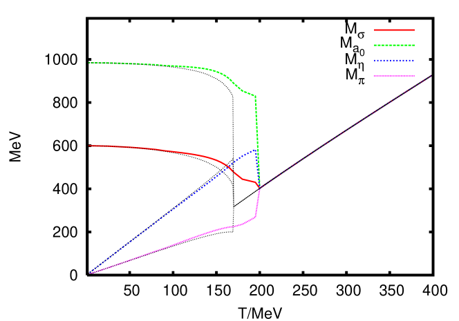
(b) Chiral limit.

Figure 10: Masses in the $U(2)_{L}\times U(2)_{R}$ model without axial anomaly as functions of temperature. Comparison of the two-loop approximation with Hartree–Fock (dotted lines).

IV.3.3 Temperature-dependent $U(1)_{A}$ anomaly

There are indications from the lattice that at high temperatures effects arising from the $U(1)_{A}$ breaking are strongly suppressed Allés et al. (1997, 1999); Chu and Schramm (1995); Chu et al. (2000); Bernard et al. (1997); Chandrasekharan et al. (1999); Gottlieb et al. (1997); Kogut et al. (1998); Chen et al. (1998). This suggests an effective restoration of the $U(1)_{A}$ symmetry close to the critical temperature. We model this by fixing the parameters at zero temperature to the physical masses but considering the anomaly parameter $c$ as a function of temperature. As an example we describe a suddenly dropping behavior at 175 MeV with the Fermi function

$$c(T)=\frac{c_{0}}{1+\exp[(T-T_{A})/\Delta T]}$$ (26)

with $T_{A}=175$ MeV and $\Delta T=10$ MeV, see Fig. 11. The values are chosen such that at $T\approx 200$ MeV the strength of the anomaly has dropped by one order of magnitude.

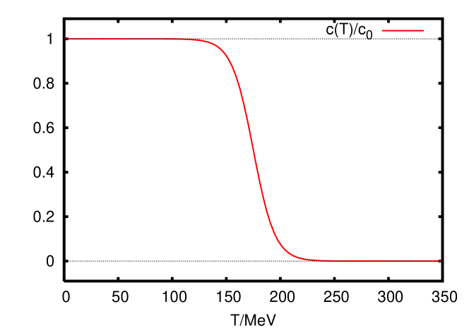
Figure 11: Modelled temperature dependence of the anomaly parameter $c$. The behavior is like the function in Eq. (26) with $T_{A}=175$ MeV and $\Delta T=10$ MeV.

This causes a sharp decrease of the order parameter at about 175 MeV, cf. Fig. 12. In the chiral limit, there is a very weak first-order transition at $T_{c}=180.49$ MeV where the condensate drops to zero from a value of $1.44$ MeV. In the Hartree–Fock approximation we find a first-order transition at $T\approx 161$ MeV. Shifting $T_{A}$ influences the order of the transition in the two-loop approximation; for $T_{A}\lesssim 175$ MeV the phase transition is of first order because the anomaly has effectively vanished at $T_{c}$, and for $T_{A}\gtrsim 175$ MeV there is a second-order transition because the axial anomaly is sufficiently strong at the critical temperature. Changing $\Delta T$ in Eq. (26) has the same effect. For explicit symmetry breaking, there is a crossover at a temperature of about $180$ MeV. The masses of the chiral partners become identical at about 200 MeV (see Fig. 13). In the two-loop approximation, these temperatures are significantly lower than those for the models with a fixed $U(1)_{A}$ anomaly. Although the anomaly parameter tends to zero the full symmetry is only finally restored at about 300 MeV where all four masses become identical. The temperature behavior of the condensate and the masses are quite similar to those found in the framework of a Nambu–Jona-Lasinio (NJL) model with three quark flavors Costa et al. (2005, 2004).

The effect that a suddenly dropping anomaly parameter triggers the restoration of chiral symmetry was observed earlier in the linear sigma model with three quark flavors Schaffner-Bielich (2000). In the chiral limit, the difference between the scalar and the pseudoscalar meson mass beyond $T_{c}$ [cf. Fig. 13(b)] is only driven by the function $c(T)$, Eq. 11. So, chiral symmetry restoration is triggered by the effective restoration of the $U(1)_{A}$ symmetry in the chiral limit, too.

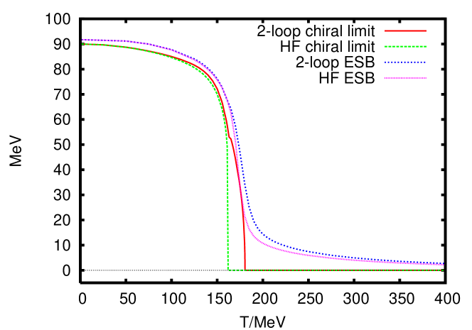
Figure 12: Temperature dependence of the condensate in the $U(2)_{L}\times U(2)_{R}$ model without an axial anomaly. Comparison of the two-loop approximation with Hartree–Fock (HF) for explicit symmetry breaking (ESB) and in the chiral limit.

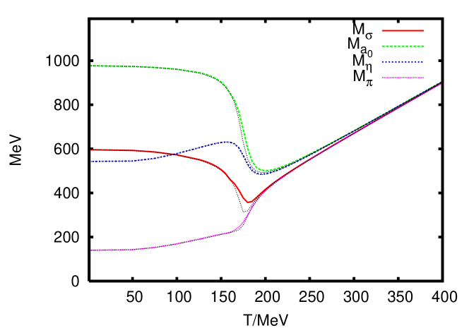
(a) Explicit symmetry breaking

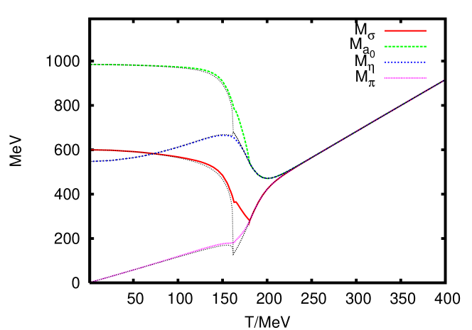
(b) Chiral limit.

Figure 13: Masses in the $U(2)_{L}\times U(2)_{R}$ model with a temperature-dependent axial anomaly as in Fig. 11. Comparison of the two-loop approximation with Hartree–Fock (dotted lines).

V Conclusions and outlook

We have investigated the restoration of chiral symmetry in the $U(2)_{L}\times U(2)_{R}$ and in the $O(N)$ linear sigma models at finite temperature. Taking into account two-loop sunset contributions makes the condensate drop less rapidly with increasing temperature; the crossover and critical temperatures are significantly higher than in the Hartree–Fock approximation which is shown in Table 4. The deviation from the Hartree–Fock approximation is induced by decay threshold effects, especially of the decay $a_{0}\to\eta\pi$, which drive the value of the condensate away from zero. For the $U(2)_{L}\times U(2)_{R}$ model with an axial $U(1)$ anomaly the masses of the chiral partners become identical at about 300 MeV for explicit symmetry breaking or at a critical temperature of about 270 MeV in the chiral limit, whereas a mass gap of $2c$ between the isospin partners remains. But even with a zero anomaly parameter, there is an effective $U(1)_{A}$ breaking by the approximation itself due to an unequal treatment of the $\eta$ meson and the pions in the gap equations (15). Here as well, the sunsets only raise the temperature where chiral symmetry is restored compared to the Hartree–Fock approximation.

We have also investigated the effect of a temperature-dependent anomaly parameter $c(T)$ as in Eq. (26). With a steep decrease at about 175 MeV, such that the strength is reduced to 10% at temperatures of about 200 MeV, we could reduce the transition temperature to 181 MeV in the chiral limit of the two-loop approximation. The phase transition is (very weakly) of first order for this parameters, though it can be changed to second order by letting $c$ decrease slower with rising temperature. The masses of the chiral partners become identical at significantly lower temperatures (about 200 MeV for explicit symmetry breaking) than with a fixed anomaly parameter. Nevertheless, the full symmetry is also only restored at about 300 MeV (explicit symmetry breaking) or at 220 MeV where both the condensate and the anomaly have vanished. Though it is obvious that a suddenly dropping anomaly parameter triggers the restoration of chiral symmetry in the two-loop approximation.

There seems to be a violation of Goldstone’s theorem in the chiral limit because all masses of the Goldstone bosons [$M_{\pi}$ in Fig. 7(b) and 13(b), $M_{\pi}$ and $M_{\eta}$ in Fig. 10(b)] are finite below the critical temperature $T_{c}$. The reason for that is the fact that resummation schemes usually violate global symmetries van Hees and Knoll (2002c). The physical masses, obtained as second derivatives of a one-particle irreducible effective potential, are not identical to the variational mass parameters. The usual geometric argument that proves the physical Goldstone masses to be zero ist the following. Consider the second derivative of a 1PI effective potential depending on the $O(N)$ invariant $\vec{\phi}^{2}=\phi_{a}\phi_{a}$

$$\frac{\partial^{2}}{\partial\phi_{a}\partial\phi_{b}}V(\vec{\phi}^{2})\biggr{|}_{\vec{\phi}=\langle\vec{\phi}\rangle}=2\,V^{\prime}(\vec{\phi}^{2})\,\delta_{ab}\biggr{|}_{\vec{\phi}=\langle\vec{\phi}\rangle}+4\,V^{\prime\prime}(\vec{\phi}^{2})\,\phi_{a}\phi_{b}\biggr{|}_{\vec{\phi}=\langle\vec{\phi}\rangle}\ .$$ (27)

With the expectation value pointing only in the $0$-direction, $\langle\vec{\phi}\rangle=(\phi_{0},0,\dots,0)$, the Goldstone masses are given by the derivatives perpendicular to that direction and thus are proportional to $V^{\prime}(\vec{\phi}^{2})$ which is zero for a non-trivial vacuum. So, whenever there is a minimum off zero in the potential there are Goldstone bosons .

Comparing this work with recent publications Röder et al. (2005); Röder (2005) one has to state that the effect of non-local corrections to the propagators seems to be more efficient for the reduction of the critical temperature from the Hartree–Fock value of about 200 MeV to a desired value of about 175 MeV Karsch (2002); Laermann and Philipsen (2003) than considering only local corrections. The approach described in this article is can only reduce the crossover temperature significantly if a varying anomaly strength is taken into account. So, it would be interesting to apply non-local resummation schemes also to the $U(2)_{L}\times U(2)_{R}$ model.

Furthermore, the effective $U(1)_{A}$ symmetry breaking that is inherent to the Hartree–Fock and two-loop approximation may be remedied by a different approximation, possibly by one inspired by a $1/N$ expansion similar to that used in Ref. Röder (2005).

Including strange mesons ($N_{f}=3$) could possibly lead to interesting non-linear effects since the $U(1)_{A}$ anomaly term is trilinear for three flavors and thus would generate additional sunset graphs with different signs. Adding fermions (nucleons or constituent quarks) to the model using a Yukawa coupling is also an attractive extension of this work Michalski (2006). For the $O(N)$ model this has been done by several authors before Roh and Matsui (1998); Mócsy et al. (2004); Caldas et al. (2001).

model			transition temperature (order of phase transition)
			Hartree–Fock	two-loop
$O(4)$		ESB	225 MeV	225 MeV
		chiral limit	181 MeV (1st)	210 MeV
$U(2)_{L}\times U(2)_{R}$	with anomaly	ESB	210 MeV	270 MeV
		chiral limit	178 MeV (1st)	272 MeV (2nd)
	without anomaly	ESB	195 MeV	245 MeV
		chiral limit	170 MeV (1st)	200 MeV (1st)
	with varying anomaly	ESB	180 MeV	185 MeV
		chiral limit	161 MeV (1st)	181 MeV (weak 1st)

Table 4: Transition temperatures and order of the phase transitions of the two models in two different approximations. For explicit symmetry breaking there is always a crossover.

Appendix A Effective action of the $U(2)_{L}\times U(2)_{R}$ model

This Appendix contains details for the computation of the effective action of the $U(2)_{L}\times U(2)_{R}$ model. We define the vacuum expectation value

$$\langle\Phi\rangle=T_{a}\,\phi_{a}$$

with a real-valued condensate $\phi_{0}$ [cf. Eq. (8)] and shift the (complex) $U(2)_{L}\times U(2)_{R}$ fields to

$$\Phi=\frac{1}{2}\phi_{0}\,\openone+T_{a}(\sigma_{a}+i\pi_{a})\ ,$$

where $\sigma_{a}$ and $\pi_{a}$ are real and symbolize the scalar and pseudoscalar meson fields. The shifted Lagrangian is a sum of four parts,

$$\mathscr{L}[\Phi]=-V_{\mathrm{class}}(\phi_{0})+\mathscr{L}_{2}[\Phi]+\mathscr{L}_{3}[\Phi]+\mathscr{L}_{4}[\Phi]\ .$$ (A1)

The first part is the classical tree-level potential

$$V_{\mathrm{class}}(\phi)=\frac{1}{2}m^{2}\phi_{a}^{2}-3\mathcal{G}_{ab}\ \phi_{a}\phi_{b}+\frac{1}{3}\mathcal{F}_{abcd}\ \phi_{a}\phi_{b}\phi_{c}\phi_{d}-h_{a}\phi_{a}\ ,$$ (A2)

which for the choice of Eq. (8) reduces to the expression in Eq. (10). The structure of the mass matrices and interactions is given by the coefficients Röder et al. (2003)

$$\mathcal{G}_{ab} = \frac{c}{6}\left(\delta_{a0}\delta_{b0}-\delta_{a1}\delta_{b1}-\delta_{a2}\delta_{b2}-\delta_{a3}\delta_{b3}\right)$$ (A3a)

$$\mathcal{F}_{abcd} = \frac{\lambda_{1}}{4}\left(\delta_{ab}\delta_{cd}+\delta_{ad}\delta_{bc}+\delta_{ac}\delta_{bd}\right)$$ (A3b)

$$+\frac{\lambda_{2}}{8}\left(d_{abn}d_{ncd}+d_{adn}d_{nbc}+d_{acn}d_{nbd}\right)$$

$$\mathcal{H}_{abcd} = \frac{\lambda_{1}}{4}\delta_{ab}\delta_{cd}+\frac{\lambda_{2}}{8}\left(d_{abn}d_{ncd}+f_{acn}f_{nbd}+f_{bcn}f_{nad}\right)\ .$$ (A3c)

The second part of the shifted Lagrangian consists of all bilinear terms in the fields

$$\begin{split}\mathscr{L}_{2}[\phi_{a};\sigma_{a},\pi_{a}]=\ &\frac{1}{2}(\partial_{\mu}\sigma_{a})^{2}-\frac{1}{2}\left[m^{2}\ \delta_{ab}-6\,\mathcal{G}_{ab}+4\,\mathcal{F}_{abcd}\ \phi_{c}\phi_{d}\right]\sigma_{a}\sigma_{b}\\ &+\frac{1}{2}(\partial_{\mu}\pi_{a})^{2}-\frac{1}{2}\left[m^{2}\ \delta_{ab}+6\,\mathcal{G}_{ab}+4\,\mathcal{H}_{abcd}\ \phi_{c}\phi_{d}\right]\pi_{a}\pi_{b}\ .\end{split}$$ (A4)

Looking at the structure of this equation we conclude that the tree-level mass matrix is diagonal if the expectation value $\phi_{a}$ has only one component, e.g., $\phi_{a}=\delta_{a0}\,\phi_{0}$. So there is neither a mass mixing among the scalar and pseudoscalar mesons nor between them. According to the 2PPI resummation scheme Smet et al. (2002); Verschelde and De Pessemier (2002); Verschelde and Coppens (1992); Baacke and Michalski (2003a) one constructs the one-loop terms as given in Eq. (11).

The third part of Eq. (A1) contains trilinear terms describing the three-particle vertex

$$\begin{split}\mathscr{L}_{3}[\phi_{a};\sigma_{a},\pi_{a}]=\ &-\frac{4}{3}\,\mathcal{F}_{abcd}\ \phi_{d}\sigma_{a}\sigma_{b}\sigma_{c}-4\,\mathcal{H}_{abcd}\ \phi_{d}\pi_{a}\pi_{b}\sigma_{c}\ .\end{split}$$ (A5)

The sunset contributions to the effective potential are constructed from that by computing the expectation value

$$V_{\text{sunset}}(M^{2},\phi_{0})=-\frac{1}{2}\left<\int_{x}\int_{y}\mathscr{L}_{3}(x)\,\mathscr{L}_{3}(y)\right>_{\text{2PPI}}$$ (A6)

where we chose conventions for Euclidean space-time and neglected an overall volume factor on the left hand side. The subscript 2PPI means that only two-particle point-irreducible graphs may be constructed from this expectation value resulting in sunset graphs with three propagators from the vertex at $x$ to the vertex at $y$ as required by Wick’s theorem. Note that since there is no tree-level mixing of masses, valid contractions are only of the type

$$\langle\sigma_{a}(x)\,\sigma_{a}(y)\rangle\longrightarrow\frac{1}{p^{2}+M_{\sigma_{a}}^{2}}\quad\text{or}\quad\langle\pi_{a}(x)\,\pi_{a}(y)\rangle\longrightarrow\frac{1}{p^{2}+M_{\pi_{a}}^{2}}$$ (A7)

where $\sigma_{0}=\sigma$, $\sigma_{1,2,3}=a_{0}$ and $\pi_{0}=\eta$, $\pi_{1,2,3}=\pi$. This finally yields the sunset contribution to the effective potential

$$\begin{split}V_{\mathrm{sunsets}}(M^{2},\phi_{0})=-\phi_{0}^{2}\,\Biggl{[}&\left(\lambda_{1}+\frac{3}{2}\lambda_{2}\right)^{2}(3\,S_{\sigma\sigma\sigma}+3\,S_{\sigma a_{0}a_{0}}+S_{\sigma\eta\eta})\\ &+\left(\lambda_{1}+\frac{\lambda_{2}}{2}\right)^{2}S_{\sigma\pi\pi}+\frac{3}{2}\lambda_{2}^{2}\,S_{a_{0}\eta\pi}\Biggr{]}\ ,\end{split}$$ (A8)

where $S_{ijk}$ denotes a sunset graph with propagators of the particles $i$, $j$ and $k$. The last part of the shifted Lagrangian contains the rest, i.e., the four-vertex interactions,

$$\begin{split}\mathscr{L}_{4}[\sigma_{a},\pi_{a}]=\ &-2\,\mathcal{H}_{abcd}\ \sigma_{a}\sigma_{b}\pi_{c}\pi_{d}-\frac{1}{3}\,\mathcal{F}_{abcd}\ (\sigma_{a}\sigma_{b}\sigma_{c}\sigma_{d}+\pi_{a}\pi_{b}\pi_{c}\pi_{d})\ .\end{split}$$ (A9)

We can now write down the general structure of the two-particle point-irreducible (2PPI) effective potential

$$V_{\mathrm{eff}}(M^{2},\phi_{0})=V_{\mathrm{class}}(\phi_{0})+2\,\mathcal{H}_{abcd}\ \Delta^{S}_{ab}\,\Delta^{P}_{cd}+\mathcal{F}_{abcd}\ (\Delta^{S}_{ab}\Delta^{S}_{cd}+\Delta^{P}_{ab}\Delta^{P}_{cd})+V_{q}(M^{2},\phi_{0})\ ,$$ (A10)

where

$$\Delta^{S}_{ab}=\langle\sigma_{a}(x)\sigma_{b}(x)\rangle\quad\text{and}\quad\Delta^{P}_{ab}=\langle\pi_{a}(x)\pi_{b}(x)\rangle$$ (A11)

denote expectation values of local composite operators (“bubbles”), and $V_{q}$ contains higher-order corrections made of 2PPI graphs likes sunsets, basketballs etc. For the masses are diagonal the expectation values (A11) are diagonal as well. Using the physical identification of the meson fields as given in Eq. (6) we declare

$$\Delta_{\sigma} \equiv\Delta^{S}_{00} \Delta_{\eta} \equiv\Delta^{P}_{00}$$ (A12a)

$$\Delta_{a_{0}} \equiv\Delta^{S}_{11}=\Delta^{S}_{22}=\Delta^{S}_{33} \Delta_{\pi} \equiv\Delta^{P}_{11}=\Delta^{P}_{22}=\Delta^{P}_{33} \ .$$ (A12b)

Contracting the coefficients $\mathcal{F}_{abcd}$ and $\mathcal{H}_{abcd}$ with the appropriate expectation values we obtain the following expression for the 2PPI effective action

$$\begin{split}V_{\mathrm{eff}}(M^{2},\phi_{0})=\ &V_{\mathrm{class}}(\phi_{0})+V_{q}(\phi_{0},M^{2})\\ &-\left(\frac{\lambda_{1}}{4}+\frac{\lambda_{2}}{8}\right)(3\,\Delta_{\sigma}^{2}+15\,\Delta_{\pi}^{2}+6\,\Delta_{\sigma}\Delta_{\pi})\\ &-\left(\frac{\lambda_{1}}{4}+\frac{\lambda_{2}}{8}\right)(3\,\Delta_{\eta}^{2}+15\,\Delta_{a_{0}}^{2}+6\,\Delta_{\eta}\Delta_{a_{0}})\\ &-\left(\frac{\lambda_{1}}{2}+\frac{\lambda_{2}}{4}\right)\Delta_{\sigma}\Delta_{\eta}+3\,\left(\frac{\lambda_{1}}{2}+\frac{3}{4}\lambda_{2}\right)\Delta_{a_{0}}\Delta_{\sigma}\\ &-3\,\left(\frac{\lambda_{1}}{2}+\frac{3}{4}\lambda_{2}\right)\Delta_{\pi}\Delta_{\eta}+3\,\left(\frac{3}{2}\lambda_{1}+\frac{7}{4}\lambda_{2}\right)\Delta_{a_{0}}\Delta_{\pi}\ ,\end{split}$$ (A13)

where $V_{\mathrm{eff}}$ is a function of the condensate $\phi_{0}$ and all four masses $M_{\sigma}$, $M_{a_{0}}$, $M_{\eta}$ and $M_{\pi}$. Note that this is the case for each quantity $\Delta_{*}$ as well since it is given by Eq. (14). Equation (A13) looks like the double-bubble term in the 2PI expansion Röder et al. (2003) except for the sign which is different here due to the special role of this contribution and the quantity $\Delta$ within the 2PPI formalism Smet et al. (2002); Verschelde and De Pessemier (2002); Verschelde and Coppens (1992).

For a detailed graphical comparison of the 2PPI and the 2PI effective action see the Appendix of Ref. Baacke and Michalski (2003a).

References

- ’t Hooft (1976a) G. ’t Hooft, Phys. Rev. Lett. 37, 8 (1976a).
- ’t Hooft (1976b) G. ’t Hooft, Phys. Rev. D14, 3432 (1976b).
- Pisarski and Wilczek (1984) R. D. Pisarski and F. Wilczek, Phys. Rev. D29, 338 (1984).
- Karsch (2002) F. Karsch, Lect. Notes Phys. 583, 209 (2002), eprint hep-lat/0106019.
- Laermann and Philipsen (2003) E. Laermann and O. Philipsen, Ann. Rev. Nucl. Part. Sci. 53, 163 (2003), eprint hep-ph/0303042.
- Fodor and Katz (2004) Z. Fodor and S. D. Katz, JHEP 04, 050 (2004), eprint hep-lat/0402006.
- de Forcrand and Philipsen (2002) P. de Forcrand and O. Philipsen, Nucl. Phys. B642, 290 (2002), eprint hep-lat/0205016.
- Gell-Mann and Levy (1960) M. Gell-Mann and M. Levy, Nuovo Cim. 16, 705 (1960).
- Dolan and Jackiw (1974) L. Dolan and R. Jackiw, Phys. Rev. D9, 3320 (1974).
- Braaten and Pisarski (1990a) E. Braaten and R. D. Pisarski, Phys. Rev. Lett. 64, 1338 (1990a).
- Braaten and Pisarski (1990b) E. Braaten and R. D. Pisarski, Nucl. Phys. B337, 569 (1990b).
- Parwani (1992) R. R. Parwani, Phys. Rev. D45, 4695 (1992), eprint hep-ph/9204216.
- Verschelde and Coppens (1992) H. Verschelde and M. Coppens, Phys. Lett. B287, 133 (1992).
- Cornwall et al. (1974) J. M. Cornwall, R. Jackiw, and E. Tomboulis, Phys. Rev. D10, 2428 (1974).
- Röder et al. (2003) D. Röder, J. Ruppert, and D. H. Rischke, Phys. Rev. D68, 016003 (2003), eprint nucl-th/0301085.
- Lenaghan et al. (2000) J. T. Lenaghan, D. H. Rischke, and J. Schaffner-Bielich, Phys. Rev. D62, 085008 (2000), eprint nucl-th/0004006.
- Schaffner-Bielich (2000) J. Schaffner-Bielich, Phys. Rev. Lett. 84, 3261 (2000), eprint hep-ph/9906361.
- Geddes (1980) H. B. Geddes, Phys. Rev. D21, 278 (1980).
- Lenaghan and Rischke (2000) J. T. Lenaghan and D. H. Rischke, J. Phys. G26, 431 (2000), eprint nucl-th/9901049.
- Baacke and Michalski (2003a) J. Baacke and S. Michalski, Phys. Rev. D67, 085006 (2003a), eprint hep-ph/0210060.
- Petropoulos (1999) N. Petropoulos, J. Phys. G25, 2225 (1999), eprint hep-ph/9807331.
- Patkós et al. (2002) A. Patkós, Z. Szép, and P. Szépfalusy, Phys. Lett. B537, 77 (2002), eprint hep-ph/0202261.
- Chiku and Hatsuda (1998) S. Chiku and T. Hatsuda, Phys. Rev. D58, 076001 (1998), eprint hep-ph/9803226.
- Nemoto et al. (2000) Y. Nemoto, K. Naito, and M. Oka, Eur. Phys. J. A9, 245 (2000), eprint hep-ph/9911431.
- Smet et al. (2002) G. Smet, T. Vanzielighem, K. van Acoleyen, and H. Verschelde, Phys. Rev. D65, 045015 (2002), eprint hep-th/0108163.
- Verschelde and De Pessemier (2002) H. Verschelde and J. De Pessemier, Eur. Phys. J. C22, 771 (2002), eprint hep-th/0009241.
- Röder et al. (2005) D. Röder, J. Ruppert, and D. H. Rischke (2005), eprint hep-ph/0503042.
- Röder (2005) D. Röder (2005), eprint hep-ph/0509232.
- Baacke and Michalski (2004a) J. Baacke and S. Michalski (2004a), eprint hep-ph/0409153.
- Baacke and Michalski (2004b) J. Baacke and S. Michalski, Phys. Rev. D70, 085002 (2004b), eprint hep-ph/0407152.
- Andersen et al. (2004) J. O. Andersen, D. Boer, and H. J. Warringa, Phys. Rev. D70, 116007 (2004), eprint hep-ph/0408033.
- de Godoy Caldas (2002) H. C. de Godoy Caldas, Phys. Rev. D65, 065005 (2002), eprint hep-th/0111194.
- van Hees and Knoll (2002a) H. van Hees and J. Knoll, Phys. Rev. D65, 025010 (2002a), eprint hep-ph/0107200.
- van Hees and Knoll (2002b) H. van Hees and J. Knoll, Phys. Rev. D65, 105005 (2002b), eprint hep-ph/0111193.
- van Hees and Knoll (2002c) H. van Hees and J. Knoll, Phys. Rev. D66, 025028 (2002c), eprint hep-ph/0203008.
- Berges et al. (2005) J. Berges, S. Borsányi, U. Reinosa, and J. Serreau, Phys. Rev. D71, 105004 (2005), eprint hep-ph/0409123.
- Blaizot et al. (2004) J.-P. Blaizot, E. Iancu, and U. Reinosa, Nucl. Phys. A736, 149 (2004), eprint hep-ph/0312085.
- Ivanov et al. (2005) Y. B. Ivanov, F. Riek, H. van Hees, and J. Knoll, Phys. Rev. D72, 036008 (2005), eprint hep-ph/0506157.
- Destri and Sartirana (2005a) C. Destri and A. Sartirana (2005a), eprint hep-ph/0509032.
- Destri and Sartirana (2005b) C. Destri and A. Sartirana, Phys. Rev. D72, 065003 (2005b), eprint hep-ph/0504029.
- Vafa and Witten (1984) C. Vafa and E. Witten, Nucl. Phys. B234, 173 (1984).
- Baacke and Michalski (2003b) J. Baacke and S. Michalski (2003b), eprint hep-ph/0312031.
- Eidelman et al. (2004) S. Eidelman et al. (Particle Data Group), Phys. Lett. B592, 1 (2004), URL http://pdg.lbl.gov.
- Baym and Grinstein (1977) G. Baym and G. Grinstein, Phys. Rev. D15, 2897 (1977).
- Bardeen and Moshe (1986) W. A. Bardeen and M. Moshe, Phys. Rev. D34, 1229 (1986).
- Allés et al. (1997) B. Allés, M. D’Elia, and A. Di Giacomo, Nucl. Phys. B494, 281 (1997), erratum-ibid. B679, 397 (2004), eprint hep-lat/9605013.
- Allés et al. (1999) B. Allés, M. D’Elia, A. Di Giacomo, and P. W. Stephenson, Nucl. Phys. Proc. Suppl. 73, 518 (1999), eprint hep-lat/9808004.
- Chu and Schramm (1995) M. C. Chu and S. Schramm, Phys. Rev. D51, 4580 (1995), eprint nucl-th/9412016.
- Chu et al. (2000) M. C. Chu, S. M. Ouellette, S. Schramm, and R. Seki, Phys. Rev. D62, 094508 (2000), eprint hep-lat/9712023.
- Bernard et al. (1997) C. W. Bernard et al., Phys. Rev. Lett. 78, 598 (1997), eprint hep-lat/9611031.
- Chandrasekharan et al. (1999) S. Chandrasekharan et al., Phys. Rev. Lett. 82, 2463 (1999), eprint hep-lat/9807018.
- Gottlieb et al. (1997) S. A. Gottlieb et al., Phys. Rev. D55, 6852 (1997), eprint hep-lat/9612020.
- Kogut et al. (1998) J. B. Kogut, J. F. Lagae, and D. K. Sinclair, Phys. Rev. D58, 054504 (1998), eprint hep-lat/9801020.
- Chen et al. (1998) P. Chen et al. (1998), eprint hep-lat/9812011.
- Costa et al. (2005) P. Costa, M. C. Ruivo, C. A. de Sousa, and Y. L. Kalinovsky, Phys. Rev. D71, 116002 (2005), eprint hep-ph/0503258.
- Costa et al. (2004) P. Costa, M. C. Ruivo, C. A. de Sousa, and Y. L. Kalinovsky, Phys. Rev. D70, 116013 (2004), eprint hep-ph/0408177.
- Michalski (2006) S. Michalski, in preparation (2006).
- Roh and Matsui (1998) H.-S. Roh and T. Matsui, Eur. Phys. J. A1, 205 (1998), eprint nucl-th/9611050.
- Mócsy et al. (2004) Á. Mócsy, I. N. Mishustin, and P. J. Ellis, Phys. Rev. C70, 015204 (2004), eprint nucl-th/0402070.
- Caldas et al. (2001) H. C. G. Caldas, A. L. Mota, and M. C. Nemes, Phys. Rev. D63, 056011 (2001), eprint hep-ph/0005180.