High energy inelastic electron hadron scattering, in peripheral kinematics. Sum rules for hadron form factors

Abstract

Relations between differential cross section for inelastic scattering of electrons on hadrons and hadron form factors (sum rules) are derived on the basis of analytical properties of heavy photon forward Compton scattering on hadrons. Sum rules relating the slope of form-factors at zero momentum transfer and anomalous magnetic moments of hadrons with some integrals on photo-production on a hadrons is obtained as well. To provide the convergence of these integrals we construct differences of individual sum rules for different hadrons. Universal interaction of Pomeron with nucleons is assumed. We derive the explicit formulae for processes of electro-production on proton and light isobar nuclei. Sudakov’s parametrization of momenta, for peripheral kinematics relevant here, is used. The light-cone form of differential cross sections is also discussed. The accuracy of sum rules estimated in frames of point-like hadrons and it is shown to be at the level of precision achievable by experiments. Suggestions and predictions for future experiments are also given.

*)On leave of absence from Istitute of Physics SAS, Bratislava

I Introduction

The idea of construction of sum rules, relating the form-factors of electron with the cross sections of electro-production processes at $e^{+}e_{-}$ high energy collisions was born in 1974. In a series of papers the cross sections of processes such as

$$e_{+}e_{-}\to(2e_{-}e_{+})e_{+};(e_{-}\gamma)e_{+};(e_{-}2\gamma)e_{+};(e_{-}\mu_{+}\mu_{-})e_{+}$$

were calculated in the so called peripheral kinematics, when the jet consisted from particles noted in parentheses are moving closely to the initial electron direction in center of mass reference frame. These cross sections do not decrease as a function of the center of mass total beam energy $\sqrt{s}$. Moreover, they are enhanced by a logarithmical factor $\ln(s/m_{e}^{2})$,which is characteristic for Weizsacker-Williams approximation. It was obtained for contribution to the process of muon pair production cross section from the so called bremsstrahlung mechanism (corresponding to the virtual photon conversion into muon - anti-muon pair) Ku74a ; Ku74b :

$$\sigma^{e^{+}e^{-}\to e^{-}\mu^{+}\mu^{-}e^{+}}=\displaystyle\frac{\alpha^{4}}{\pi\mu^{2}}\left[\left(ln\displaystyle\frac{s^{2}}{m_{e}^{2}\mu^{2}}\right)\left(\displaystyle\frac{77}{18}\xi_{2}-\displaystyle\frac{1099}{162}\right)+const\right]$$ (1)

where $\xi_{2}=\displaystyle\frac{\pi^{2}}{6}$.

In the paper of Barbieri,Mignaco and Remiddi Ba72 from 1972 the slope of the electron Dirac Form Factor for $q^{2}\to 0$ was calculated :

$$F_{1}^{\prime}(0)=\displaystyle\frac{\alpha^{2}}{8\pi^{2}\mu^{2}}\left(\displaystyle\frac{77}{18}\xi_{2}-\displaystyle\frac{1099}{162}\right).$$ (2)

The fact that the same coefficients appear in Eqs (1) and (2) suggests that a relation exists between inelastic cross section and elastic form factors. This relation was later on derived in the paper Ku74b .

Here we review an extension of these studies to strong interaction particles, considering QED interactions in the lowest order of perturbation theory. We demonstrate sum rules which relate the nucleon and light nuclei form-factors with the differential cross sections of electron scattering on the corresponding hadrons in peripheral kinematics. This kinematics corresponds to the region of very small values of Bjorken parameter $x_{B}$ in deep inelastic scattering experiments. This paper is organized as follows.

After describing the relevant processes in peripheral kinematics, in terms of Sudakov variables (Section II), we remind the analytical properties of the advanced and the retarded parts of the virtual Compton scattering amplitudes (Section II). Then briefly the problem of restoring gauge invariance and formulation of the modified optical theorem are discussed.

Following QED analysis in Ku74b , we introduce light cone projection of Compton scattering amplitude integrated on some contour in the $s_{2}$ plane, where $s_{2}$ is the invariant mass squared of the hadronic jet.

Sum rules (Section III) arise when the Feynman contour in the $s_{2}$ plane is closed to the left real axes singularities of the Compton amplitude and to the right ones. Sum rules obtained in such a way contain the left hand cut contribution which is difficult to be interpreted in terms of cross sections. Moreover, it suffers from ultraviolet divergencies of contour integral arising from Pomeron Regge pole contribution. The final form of these sum rules consists of differences, constructed in such a way in order to compensate the Pomeron contributions and the left hand cuts as well.

The applications to different kinds of targets, as proton and neutron, deuteron and light nuclei are explicitly given. Appendix A is devoted to an estimation of the cross section of $p\bar{p}$ pair proton photo-production in the framework of a simple model arising from effect of identity of protons in final state. In Appendix B the details of kinematics of recoil target particle momentum is investigated in terms of Sudakov’s approach.

I.1 Sudakov parametrization

Let us consider the process presented in Fig. 1, where the inelastic electron - hadron interaction occurs through a virtual photon of momentum $q$. The particle momenta are indicated in the figure: $p^{2}=M^{2}$, $p_{1}^{2}=p_{1}^{\prime 2}=m^{2}$. The total energy is $s=(p+p_{1})^{2}$ and the momentum transfer from the initial to the final electron is $t=(p_{1}-p_{1}^{\prime})^{2}$.

Let us introduce some useful notations, in order to calculate the differential cross section for the process of Fig. 1, where the the hadron is a proton in peripheral kinematics, i.e, $s\gg-t\simeq M^{2}$. Therefore $s=(p_{1}+p)^{2}=M^{2}+m_{e}^{2}+2pp_{1}\simeq 2pp_{1}=2ME\gg M^{2}\gg m_{e}^{2}$.

The differential cross section can be written as:

$$d\sigma=\displaystyle\frac{1}{2\cdot 2\cdot 2s}\sum|{\cal M}|^{2}d\Gamma.$$ (3)

Let us define two light-like vectors:

$$\tilde{p}=p-p_{1}\displaystyle\frac{M^{2}}{s},~{}\tilde{p}_{1}=p_{1}-p\displaystyle\frac{m^{2}}{s}$$

and a transversal vector, $q_{\perp}$, such that $\tilde{p}q_{\perp}=p_{1}q_{\perp}=0.$

Therefore ${\tilde{p}}^{2}={\cal O}\left(\displaystyle\frac{m^{2}M^{4}}{s^{2}}\right)$ and similarly ${\tilde{p}}^{2}={\cal O}\left(\displaystyle\frac{m^{4}M^{2}}{s^{2}}\right)$. Terms of order ${\cal O}\left(\displaystyle\frac{M^{2}}{s},\frac{m^{2}}{M^{2}}\right)$ compared to ones of order 1 we will neglect systematically. In the Laboratory system, with an appropriate choice of the axis, the four vectors are written, in explicit form, as: $\tilde{p}_{1}\approx p_{1}=E(1,1,0,0)$, and $\tilde{p}=\displaystyle\frac{M}{2}(1,-1,0,0)$, and $q_{\perp}=(0,0,q_{x},q_{y})$, $q^{2}_{\perp}=-\vec{q}^{2}<0$, which is essentially a two-dimensional vector. Let us express the four momentum of the exchanged photon in the Sudakov parametrization, in infinite momentum frame, as function of two (small) parameters $\alpha$ and $\beta$ (Sudakov parameters):

$$q=\alpha\tilde{p}+\beta\tilde{p}_{1}+q_{\perp}.$$ (4)

The on-mass shell condition for the scattered electron can be written as:

$$p_{1}^{\prime 2}-m^{2}=(p_{1}-q)^{2}-m^{2}=-\vec{q}^{2}+s\alpha\beta-\alpha s-\beta m^{2}=0$$ (5)

where we use the relation:

$$2p_{1}\tilde{p}_{1}=2p_{1}\left(p_{1}-p\displaystyle\frac{m^{2}}{s}\right)=m^{2},$$ (6)

similarly one can find $2p\tilde{p}=M^{2}$.

From the definition, Eq. (4), and using Eq. (5), the momentum squared of the virtual photon is:

$$q^{2}=s\alpha\beta-\vec{q}^{2}=-\displaystyle\frac{\vec{q}^{2}+m^{2}\beta^{2}}{1-\beta}<0.$$

The variable $\beta$ is related to the invariant mass of the proton jet, the set of particles moving close to the direction of the initial proton:

$$s_{2}=(q+p)^{2}-M^{2}+{\vec{q}}^{2}\simeq s\beta$$

neglecting small terms as $s\alpha\beta$ and $\alpha M^{2}$ (Weizsacker-Williams approximation We34 ). We discuss later the consequences of such approximation on the $s$ dependence of the cross section. In these notation the phase space of the final particle

$$d\Gamma = (2\pi)^{4}\displaystyle\frac{d^{3}p_{1}^{\prime}}{2\epsilon_{1}^{\prime}(2\pi)^{3}}\Pi_{1}^{n}\displaystyle\frac{d^{3}q_{i}}{2\epsilon_{i}(2\pi)^{3}}\delta^{4}(p_{1}+p-p_{1}^{\prime}-\sum_{i}^{n}q_{i}),$$ (7)

introducing an auxiliary integration on the photon transferred momentum $\int d^{4}q\delta^{4}(p_{1}-q-p_{1}^{\prime})=1$ can be written as

$$d\Gamma=(2\pi)^{-3}\delta^{4}((p_{1}-q)^{2}-m^{2})d^{4}qd\Gamma_{H},$$ (8)

where $d\Gamma_{H}$ is the hadron phase space:

$$d\Gamma_{H}=(2\pi)^{4}\delta^{4}(p+q-\sum_{i}^{n}q_{i})\Pi_{1}^{n}\displaystyle\frac{d^{3}q_{i}}{2\epsilon_{i}(2\pi)^{3}}.$$ (9)

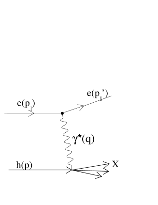
Figure 1: Feynman diagram for inelastic electron hadron scattering .

In the Sudakov parametrization:

$$d^{4}q=\displaystyle\frac{s}{2}d\alpha d\beta d^{2}q_{\perp}\simeq\displaystyle\frac{ds_{2}}{2s}d(s\alpha)d^{2}\vec{q},$$ (10)

we obtain:

$$d\Gamma=\displaystyle\frac{ds_{2}}{2s}d^{2}\vec{q}(2\pi)^{-3}d\Gamma_{H}.$$ (11)

Let us use the matrix elements to be expressed by the Sudakov parameters. Then it can be rewritten into the form:

$${\cal M}=\displaystyle\frac{4\pi\alpha}{q^{2}}\overline{u}(p_{1}^{\prime})\gamma^{\mu}u(p_{1}){\cal J}_{H}^{\nu}g_{\mu\nu}.$$ (12)

It is convenient to use here the Gribov representation of the numerator of the (exact) Green function in the Feynman gauge for the exchanged photon:

$$g_{\mu\nu}=(g_{\perp})_{\mu\nu}+\displaystyle\frac{2}{s}(\tilde{p}_{\mu}\tilde{p}_{1\nu}+\tilde{p}_{\nu}\tilde{p}_{1\mu}).$$ (13)

All three terms, in the right hand side of the previous equation, give contributions to the matrix element proportional to

$$1:\displaystyle\frac{s}{M^{2}}:\displaystyle\frac{M}{s}.$$

So, the main contribution (with power accuracy) is

$${\cal M}=\displaystyle\frac{4\pi\alpha}{q^{2}}\displaystyle\frac{2}{s}{\overline{u}}(p_{1}^{\prime})\hat{p}u(p_{1}){\cal J}_{H}^{\nu}p_{1\nu}=\displaystyle\frac{8\pi\alpha s}{q^{2}}N\displaystyle\frac{{\cal J}_{H}^{\nu}p_{1\nu}}{s},$$ (14)

with $N=\displaystyle\frac{1}{s}{\overline{u}}(p_{1}^{\prime})\hat{p}u(p_{1})$. One can see explicitly the proportionality of the matrix element of peripheral processes to $s$, in the high energy limit, $s\gg-t$. It follows from the relation $\sum_{pol}|N|^{2}=\displaystyle\frac{1}{s^{2}}Tr\hat{p}_{1}^{\prime}\hat{p}\hat{p}_{1}\hat{p}=2$ and from the fact, that the quantity $\displaystyle\frac{1}{s}{\cal J}_{H}^{\nu}p_{1\nu}$ is finite in this limit. Such term can be further transformed using the conservation of the hadron current ${\cal J}_{H}^{\nu}q_{\nu}\simeq(\beta p_{1}+q_{\perp})_{\nu}{\cal J}_{H}^{\nu}=0$. The latter leads to

$$\frac{1}{s}{\cal J}_{H}^{\nu}p_{1\nu}=\displaystyle\frac{1}{s\beta}\vec{q}\cdot\vec{\cal J}_{H}=\displaystyle\frac{|\vec{q}|}{s_{2}}(\vec{e}\cdot\vec{\cal J}_{H}),$$ (15)

where $\vec{e}=\vec{q}/|\vec{q}|$ is the polarization vector of the virtual photon. As a result, one finds:

$$\sum|{\cal M}|^{2}=\displaystyle\frac{(8\pi\alpha s)^{2}|\vec{q}|^{2}}{\left[(\vec{q})^{2}+m^{2}\left(\displaystyle\frac{s_{2}}{s}\right)^{2}\right]^{2}}\displaystyle\frac{2}{s_{2}^{2}}\left(\vec{\cal J}_{H}\cdot\vec{e}\right)^{2}.$$ (16)

With the help of Eqs. (7,14,16) one finds:

$$d\sigma^{(e+p\to e+jet)}=\displaystyle\frac{\alpha^{2}d^{2}q\vec{q}^{2}ds_{2}}{\pi\left[(\vec{q})^{2}+m^{2}\left(\displaystyle\frac{s_{2}}{s}\right)^{2}\right]^{2}s_{2}^{2}}(\vec{e}\cdot\vec{\cal J}_{H})^{2}d\Gamma_{H}.$$ (17)

Let us note that the differential cross section at $\vec{q}^{2}\neq 0$ does not depend on the CMS energy $\sqrt{s}$. In the logarithmic (Weizsacker-Williams) approximation, the integral over the transverse momentum $\vec{q}$, at small $\vec{q}^{2}$, gives even rise to large logarithm:

$$\sigma_{tot}^{\ell}=\pi\alpha~{}ln\left(\displaystyle\frac{s^{2}Q^{2}}{M^{4}m^{2}}\right)\int_{s_{th}}^{\infty}\displaystyle\frac{ds_{2}}{s_{2}}\sigma_{tot}^{(\gamma+p\to X)}(s_{2}),$$ (18)

where $s_{th}=(M+m_{\pi})^{2}-M^{2}$, $Q^{2}$ is the characteristic momentum transfer squared, $Q^{2}\simeq M^{2}$, and we introduced the total cross section for real polarized photons interacting with protons:

$$\sigma_{tot}^{(\gamma+p\to X)}(s_{2},q^{2}=0)=\displaystyle\frac{\alpha\pi}{s_{2}}\int(\vec{\cal J}_{H}\cdot\vec{e})^{2}d\Gamma_{H}.$$ (19)

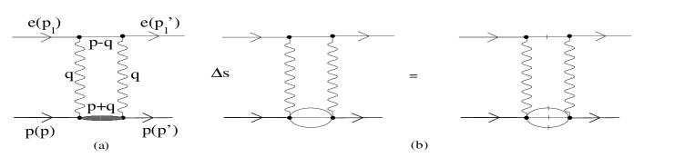
Figure 2: Feynman diagram for $e^{+}e^{-}$ scattering at the order $\alpha^{3}$.

The differential cross section $(\ref{eq:qq3})$ is closely related (due to the optical theorem) with the $s$-channel discontinuity of the forward amplitude for electron-proton scattering with the same intermediate state: a single electron and a jet, moving in opposite directions (see Figs. 2a, 2b) where, by Cutkovsky rule, the denominators of the ”cutted” lines in the Feynman graph of Fig. 2b must be replaced by:

$$\frac{1}{q^{2}-M^{2}+i0}\to-2\pi i\delta(q^{2}-m^{2}).$$ (20)

For the spin averaged forward scattering amplitude we have:

$$\Delta_{s}A(s)=\displaystyle\frac{4s\alpha}{\pi^{2}}\int\displaystyle\frac{d^{2}q_{\perp}\vec{q}^{2}}{(q^{2})^{2}}\int\displaystyle\frac{ds_{2}}{s_{2}}\sigma^{(\gamma^{*}p\to X)}(s_{2},q)$$ (21)

with

$$\sigma^{(\gamma^{*}p\to X)}(s_{2},q)=\int\displaystyle\frac{4\pi\alpha}{2\cdot 2\cdot 2s_{2}}(\vec{\cal J}_{H}\cdot\vec{e})^{2}d\Gamma_{H}.$$ (22)

From the formulae given above we can obtain

$$\frac{d\Delta_{s}\bar{A}^{eY\to eY}}{d^{2}q}=2s\frac{d\sigma^{eY\to eY}}{d^{2}q},$$ (23)

where $\bar{A}^{eY\to eY}$ is the averaged on spin states forward scattering amplitude. This relation is the statement of optical theorem in differential form.

Let us now consider the discontinuity of forward scattering amplitude with the initial hadron intermediate state, we call it a ”pole contribution”. For the case of elastic electron-proton scattering we have

$$\frac{d\Delta_{s}\bar{A}^{ep\to ep}}{d^{2}q}=\frac{(4\pi\alpha)^{2}}{(q^{2})^{2}s(2\pi)^{2}}Sp,$$ (24)

with

$$Sp=Sp(\hat{P}+M_{p})\Gamma(q)(\hat{P}^{\prime}+M_{p})\Gamma(-q)^{*},$$

and

$$\Gamma(q)=F_{1}\hat{p}_{1}-\frac{1}{2M}F_{2}\hat{q}\hat{p}_{1}.$$

A simple calculation gives $Sp=2s^{2}[(F_{1})^{2}+\tau(F_{2})^{2}]$, with $\tau=\vec{q}^{2}/(4M^{2}_{p})$.

For the case of electron-deuteron scattering we use the electromagnetic vertex of deuteron in the form AR78

$$<\xi^{\lambda^{\prime}}(P^{\prime})|J^{EM}_{\mu}(q)|\xi^{\lambda}(P)>=d_{\mu}[F_{1}(\xi^{\lambda^{\prime}*}\xi^{\lambda})-\frac{F_{3}}{2M_{d}^{2}}(\xi^{\lambda^{\prime}*}q)(\xi^{\lambda}q)]+F_{2}[\xi^{\lambda}_{\mu}(q\xi^{\lambda^{\prime}*})-\xi^{\lambda^{\prime}*}_{\mu}(\xi^{\lambda}q)],$$ (25)

where $d_{\mu}=(P^{\prime}+P)_{\mu},q_{\mu}=(P^{\prime}-P)_{\mu}$ and $\xi^{\lambda}(P)$ is the polarization vector of deuteron in chiral state $\lambda$. It has the properties:

$$\xi^{2}=-1,(\xi(P)P)=0;\sum_{\lambda}\xi^{\lambda}(P)_{\mu}\xi^{\lambda*}(P)_{\nu}=g_{\mu\nu}-\frac{P_{\mu}P_{\nu}}{M_{d}^{2}}.$$ (26)

For the averaged on spin states forward scattering amplitude we have

$$\frac{d\Delta_{s}\bar{A}^{ed\to ed}}{d^{2}q}=\frac{2s(4\pi\alpha)^{2}}{3(q^{2})^{2}(2\pi)^{2}}Tr,$$ (27)

with

$$Tr=2(F_{1})^{2}+(F_{1}+2\tau_{d}(1+\tau_{d})F_{3})^{2}+2\tau_{d}(F_{2})^{2},\tau_{d}=\frac{\vec{q}^{2}}{4M_{d}^{2}}.$$ (28)

We note that the amplitude corresponding to box-type Feynman diagram with the crossed photon legs have a zero $s$-channel discontinuity.

II Virtual Compton scattering on proton

Let us examine the different contributions to the total amplitude for virtual photon Compton scattering on a proton (hadron). Keeping in mind the baryon number conservation low we can separate all possible Feynman diagram to four classes. In one, which will be named as class of retarded diagram (corresponding amplitude is denoted as $A_{1}$) the initial state photon is first absorbed by nucleon line and after emitted the scattered photon. Another class (advanced, $A_{2}$), corresponds to the diagrams, in which scattered photon is first emitted along the nucleon line and the point of absorption is located after. Third class corresponds to the case when both photons do not interact with initial nucleon line. The corresponding amplitude is which we denote as $A_{P}$. The fourth class contains diagrams in which only one of external photons interact with nucleon line. The corresponding notation is $A_{odd}$ (see Fig.3):

$$A^{\mu\nu}(s,q)=A_{1}^{\mu\nu}(s,q)+A_{2}^{\mu\nu}(s,q)+A_{P}^{\mu\nu}(s,q)+A_{odd}.$$ (29)

Amplitude $A_{P}^{\mu\nu}(s,q)$ corresponds to Pomeron type Feynman diagram (Fig. 4e) and gives the non-vanishing contribution to the total cross sections in the limit of a large invariant mass squared of initial particles $s_{2}\to\infty$. The fourth class amplitude can be relevant in experiments with measuring the charge-odd effects. It is not considered here. One can show explicitly that each of 4 classes amplitudes are gauge invariant. The arguments in favor of it is essentially the same as was used in QED case BFKK .

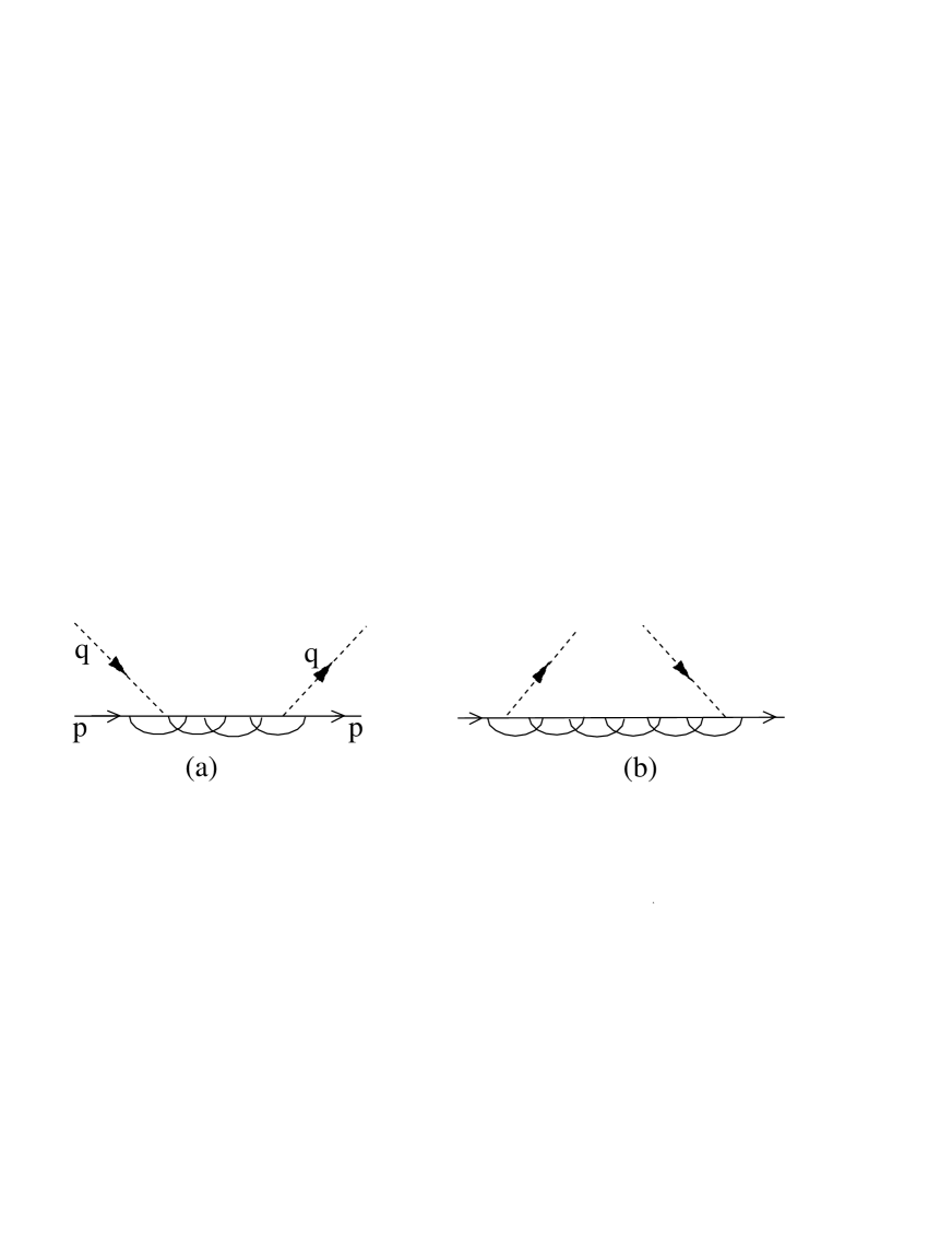
Figure 3: Illustration of retarded (a) and advanced (b) virtual photon emission and absorbtion diagrams. The diagram containing Pomeron is not considered here.

Let us discuss now the analytical properties of the retarded part of the forward Compton scattering of a virtual photon on a proton, $A_{1}(s_{2},q)$ (see Fig. 4)at $s_{2}$ - plane. Due to general principles the singularities - poles and branch points - are situated on the real axis.

These singularities are illustrated in Fig. 5. On the right side the pole at $s_{2}=0$ correspond to one nucleon exchange in the $s_{2}$ channel (Fig. 5a), the right hand cut starts at the pion-nucleon threshold, $s_{2}=(M+m_{\pi})^{2}-M^{2}$. The left cut, related with the $u$ channel 3-nucleon state of the Feynman amplitude is illustrated in Fig. 4f. It is situated rather far from the origin at $s_{2}=-8M^{2}$. It can be shown that it is the nearest singularity of right hand cut. Really the $u$-channel cut corresponding to $2\pi N$ state can not be realized without exotic quantum number states (see Fig. 4h).

III Sum rules

Following to BFKK let us introduce the quantity

$$\int_{C}ds_{2}\displaystyle\frac{p_{1}^{\mu}p_{1}^{\nu}A_{1\mu\nu}^{\gamma^{*}p\to\gamma^{*}p}}{s^{2}({\vec{q}}^{2})^{2}}=\displaystyle\frac{dI}{d{\vec{q}}^{2}},$$ (30)

with the Feynman contour $C$ in the $s_{2}$ plane as it is shown in Fig. 5a.

Sum rules appear when one considers the equality of the path integrals along the contours obtained by deformation $C$ such to be closed to the left and to the right side (Fig. 5). As a result one finds:

$$F({\vec{q}}^{2})=\displaystyle\frac{d\sigma_{left}}{d{\vec{q}}^{2}}-\displaystyle\frac{d\sigma_{el}-d\sigma_{el}^{B}}{d{\vec{q}}^{2}}=\displaystyle\frac{d\sigma_{inel}}{d{\vec{q}}^{2}},$$ (31)

where $\displaystyle\frac{d\sigma_{left}}{d{\vec{q}}^{2}}$ indicates the contribution of left cut ;

$$\frac{d\sigma_{el}^{B}}{d{\vec{q}}^{2}}=\displaystyle\frac{4\pi\alpha^{2}Z^{2}}{({\vec{q}}^{2})^{2}}.$$

The latter is generally the Born cross section of the scattering of an electron on any hadron with charge $Z$, when the strong interaction is switched off, and $\displaystyle\frac{d\sigma_{el}}{d{\vec{q}}^{2}}$ is the elastic electron hadron cross section, when the strong interaction is switched on, in the lowest order of QED coupling constant. This quantity can be expressed in terms of electromagnetic form factors of corresponding hadrons.

Using the notation for generalized square of form-factors as $\Phi^{2}$ we have for process of electron scattering on a hadron $Y$ with charge $Z$ the expression:

$$Z^{2}-\Phi^{2}(-\vec{q}^{2})=\frac{2\vec{q}^{2}}{\pi\alpha^{2}}\frac{d\sigma^{eY\to eX}}{d\vec{q}^{2}}.$$ (32)

For the case of spin-zero target the quantity $\Phi^{2}$ coincide with its squared charge form factor.

For the case of electron scattering on a spin one-half (proton, ${}^{3}\!He$,${}^{3}\!H$),which are described by two form-factors (Dirac’s one $F_{1}$ and Pauli one $F_{2}$) we have

$$Z_{i}^{2}-F_{1i}^{2}(-\vec{q}^{2})-\tau_{i}F_{2i}^{2}(-\vec{q}^{2})=\frac{2\vec{q}^{2}}{\pi\alpha^{2}}\frac{d\sigma^{eY_{i}\to eX_{i}}}{d\vec{q}^{2}},$$ (33)

with

$$\tau_{i}=\frac{\vec{q}^{2}}{4M_{i}^{2}};Z_{p}=Z_{{}^{3}\!H}=1;Z_{{}^{3}\!He}=2.$$

For scattering of electron on deuteron we have:

$$1-\frac{1}{3}[2F_{1}^{2}(-\vec{q}^{2})+[F_{1}(-\vec{q}^{2})+2\tau_{d}(1+\tau_{d})F_{3}(-\vec{q}^{2})]^{2}+2\tau_{d}F_{2}^{2}(-\vec{q}^{2})]=\frac{2\vec{q}^{2}}{\pi\alpha^{2}}\frac{d\sigma^{ed\to eX}}{d\vec{q}^{2}}.$$ (34)

These equations can be tested in experiments with electron-hadron colliders.

Further we will consider differential form of these sum rules: $\left.\displaystyle\frac{d}{d{\vec{q}}^{2}}({\vec{q}}^{2})^{2}F({\vec{q}}^{2})\right|_{{\vec{q}}^{2}=0}$, which can be expressed in terms of charge radii of hadrons, their anomalous magnetic moments, etc. and photo-production total cross section.

Considering formally this derivative at $\vec{q}^{2}=0$ we obtain

$$\frac{d}{d\vec{q}^{2}}\Phi_{Y}^{2}|_{\vec{q}^{2}=0}=\frac{2}{\pi^{2}\alpha}\int\limits_{s_{th}}^{\infty}\frac{ds_{2}}{s_{2}}\sigma_{tot}^{\gamma Y\to X}(s_{2}).$$ (35)

Unfortunately the sum rule in this form can not be used for experimental verification due to the divergence of integral in right hand side of this equation. Its origin follows from the known fact of increasing of photo production cross sections at large values of initial center of mass energies squares $s_{2}$. It’s commonly known that this fact is the consequence of Pomeron Regge pole contribution. The universal character of Pomerom interaction with nucleons can be confirmed by the Particle Data Group-2004 (PDG) result

$$[\sigma^{\gamma p}(s_{2})-\sigma^{\gamma n}(s_{2})]|_{s_{2}\to\infty}=[2\sigma^{\gamma p}(s_{2})-\sigma^{\gamma d}(s_{2})]|_{s_{2}\to\infty}=0.$$ (36)

In paper Ba04 the difference of proton and neutron sum rule was derived

$$\frac{1}{3}<r^{2}_{p}>+\displaystyle\frac{1}{4M^{2}}\left[\kappa^{2}_{n}-\kappa^{2}_{p}\right]=\displaystyle\frac{2}{\pi^{2}\alpha}\int_{\omega_{n}}^{\infty}\displaystyle\frac{d\omega}{\omega}\left[\sigma^{\gamma p\to X}(\omega)-\sigma^{\gamma n\to X}(\omega)\right].$$ (37)

We use here the known relations

$$F_{1}(-\vec{q}^{2})=1-\frac{1}{6}\vec{q}^{2}<r^{2}>+O((\vec{q}^{2})^{2});F_{2}(0)=\kappa,$$

with $<r^{2}>,\ \kappa$-are the charge radius squared and the anomalous magnetic moment of nucleon (in units $h/Mc$).

It was verified in this paper that this sum rule is fulfilled within the experimental errors: both sides of the equation equal 1.925 mb. Here the Pomeron contribution is compensated in the difference of proton and neutron total cross photo-production cross sections.

In paper Du06 the similar combination of cross sections was considered for A=3 nuclei:

$$\frac{2}{3}<r^{2}_{{}^{3}\!He}>-\displaystyle\frac{1}{3}<r^{2}_{{}^{3}\!H}>-\displaystyle\frac{1}{4M^{2}}\left[\kappa^{2}_{{}^{3}\!He}-\kappa^{2}_{{}^{3}\!H}\right]=\displaystyle\frac{2}{\pi^{2}\alpha}\int_{\omega_{th}}^{\infty}\displaystyle\frac{d\omega}{\omega}\left[\sigma^{\gamma^{3}\!He\to X}(\omega)-\sigma^{\gamma^{3}\!H\to X}(\omega)\right].$$ (38)

In the similar way, the combination of cross sections of electron scattering on proton and deuteron leads to the relation

$$\frac{1}{3}<r^{2}_{d}>-\frac{F_{3}(0)}{3M_{d}^{2}}-\frac{1}{6M_{d}^{2}}F_{2}(0)^{2}-2[\frac{1}{3}<r^{2}_{p}>-\frac{1}{4M_{p}^{2}}\kappa_{p}^{2}]=$$

$$\frac{2}{\pi^{2}\alpha}\int\limits_{\omega_{th}}^{\infty}\frac{d\omega}{\omega}[\sigma_{tot}^{\gamma d\to X}(\omega)-2\sigma_{tot}^{\gamma p\to X}(\omega)],$$ (39)

with $\omega_{th}$ for deuteron and proton are different: $(\omega_{th})_{d}=2,2MeV,(\omega_{th})_{p}=m_{\pi}+\frac{m_{\pi}^{2}}{2M_{p}}\approx 140MeV.$

We use here the similar expansion for $F_{1}$ deuteron form factor $F_{1}(0)=1$ and introduce its square charge radius. Other quantities can be found in paper GM :

$$F_{2}(0)=-\frac{M_{d}}{M_{p}}\mu_{d};\ \mu_{d}=0.857;\ 2F_{3}(0)=1+F_{2}(0)-M_{d}^{2}Q_{d};\ Q_{d}=0.2859fm^{2}.$$

We find for the left side of formula (39) by using PDG-2000 and rossi

$$\frac{2}{\pi^{2}\alpha}\biggl{\{}\int\limits_{0.020}^{0.260}\frac{d\omega}{\omega}\sigma_{tot}^{\gamma d\to X}(\omega)+\int\limits_{0.260}^{16}\frac{d\omega}{\omega}\biggl{[}\sigma_{tot}^{\gamma d\to X}(\omega)-2\sigma_{tot}^{\gamma p\to X}(\omega)\biggr{]}\biggr{\}}=0.8583fm^{2}=8.5834mb$$ (40)

IV Conclusions

The left cut contribution has no direct interpretation in terms of cross section. In analogy with QED case it can be associated with contribution to the cross section of process of proton antiproton pair electro-production on proton $ep\to e{2p\bar{p}}$, arising from taking into account the identity of final state protons.

Fortunately the threshold of this process is located enough far away. Using this fact we can estimate its contribution in the framework of QED- like model with nucleons and pions ($\rho$-mesons),omitting the form factor effects (so we put them equal to coupling constants of nucleons with pions and vector mesons).

In this paper we use optical theorem, which connects the s-channel discontinuity of forward scattering amplitude with the total cross section. This statement is valid for complete scattering amplitude, nevertheless, we consider only part of it, $A_{1}$. We can explicitly point out on the Feynman diagram (see Fig. 4 g), contributing to $A_{2}$, which has 3 nucleon $s$-channel state. The relevant contribution can be interpreted as identity effect of proton photo-production of $p\bar{p}$ pair.

The explicit calculation in the framework of our approach is given by Appendix A. The corresponding contribution to the derivative on $\vec{q}^{2}$ at $\vec{q}^{2}=0$ of scattering amplitudes entering the sum rules have an order of magnitude

$$I=\frac{g^{4}M^{2}}{\pi^{3}s_{2min}^{2}}.$$

In order to estimate the strong coupling constant we use the PDG value for the total cross section of scattering of pion on proton $\sigma_{tot}^{\pi p}=20mb$. Keeping in mind the $\rho$-meson t-channel contribution $\sigma^{\pi p}\sim g^{4}/(4\pi m_{\rho}^{2})$ and the minimal value of three nucleon invariant mass squared $s_{2min}=8M_{p}^{2}$ we have $I\approx(1/15)mb$. Comparing this value with typical values of right and left hand sides of sum rules of order of $2mb$ we estimate the error arising by omitting the left cut contribution as well as replacing our non-complete cross section by the measurable ones on the level of $3\%$.

Using the data and PDG (2000) for $\gamma p$ and $\gamma d$ cross sections rossi we find

$$<r_{d}>\ \approx\ 1.94fm.$$

This quantity in a satisfactory agreement with prediction of models based dispersion relations d where is $<r_{d}>\sim 2fm.$ Reason (besides the errors 3% of our approach) can be related with the lack of data for $\gamma p$ and $\gamma d$ cross sections near the thresholds.

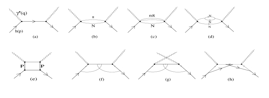
Figure 4: Feynman diagrams for forward virtual Compton scattering on the proton, contributing to the retarded part of the amplitude: intermediate state in $s_{2}$ channel for single proton (a), $N\pi$ (b), $Nn\pi$ (c), $\sum N\overline{N}$ (d), two jets $s_{2}$ channel state, with two Pomeron $t$ channel state (d), $3N$ intermediate state in $u$ channel (e), $3N$ intermediate state in $u_{2}$ channel (f). The Feynman diagram of the $A_{2}$ set which has $s$ channel discontinuity is illustrated in (g) and an example of exotic $u$ channel state in (h).

Figure 5: Illustration of singularities along the $s_{2}$ real axis with the open contour C (a), and with the contour C closed (b), corresponding o Fig. 4. LC stays for large circle contribution.

V Acknowledgement

The authors are thankful to S.Dubnicka for careful reading of the manuscript and valuable discussions. One of us (E.K.) is grateful to the Institute of Physics, Slovak Academy of Sciences, Bratislava for warm hospitality and (M.S.) is grateful to Slovak Grant Agency for Sciences VEGA for partial support, Gr.No. 2/4099/25. One of us (E.K) is grateful to Saclay Physical Centrum, Paris, where part of this work was done. We are grateful to A. V. Shebeko (KHFIT, Kharkov, Ukraina) and V. V. Burov (JINR) for detailed information about deuteron disintegration region kinematics.

VI Appendix A:effect of identity of protons to the cross section of $2p\bar{p}$ photo-production cross section

The contribution to s-channel discontinuity of part $A_{2}^{\gamma^{*}p\to\gamma^{*}p}$ scattering amplitude arising from interference of amplitudes of creation of proton-antiproton pair bremsstrahlung type due to identity of protons in the final state have a form:

$$\Delta_{s}A_{2}(s,q)=-\frac{16g^{4}}{s^{2}}\int ds_{2}d\Gamma_{3}\frac{S}{(q_{1}^{2}-m_{\pi}^{2})(q_{2}^{2}-m_{\pi}^{2})},$$ (41)

where $q_{1}=P_{1}-P,q_{2}=P_{2}-P$ and

$$S=\frac{1}{4}Sp(\hat{P}+M)\gamma_{5}(\hat{P}_{1}+M)V_{1}(\hat{P}_{3}-M)V_{2}(\hat{P}_{2}+M)\gamma_{5},$$

and $V_{1}=\gamma_{5}\frac{\hat{q}-\hat{P}_{3}+M}{d_{3}}\hat{p}_{1}+\hat{p}_{1}\frac{\hat{P}_{1}-\hat{q}+M}{d_{1}}\gamma_{5}$;
$V_{2}=\gamma_{5}\frac{-\hat{q}+\hat{P}_{2}+M}{d_{2}}\hat{p}_{1}+\hat{p}_{1}\frac{-\hat{P}_{3}+\hat{q}+M}{d_{3}}\gamma_{5}$;
$d_{1,2,3}=(q-P_{1,2,3})^{2}-M^{2},s_{2}=(P+q)^{2}-M-q^{2}$.

Besides the phase volume element have a form:

$$d\Gamma_{3}=(2\pi)^{4}\delta^{4}(P+q-P_{1}-P_{2}-P_{3})\Pi_{1}^{3}\frac{d^{3}P_{i}}{2E_{i}(2\pi)^{3}}.$$

Here we consider pions to be interacting with nucleons with coupling constant $g$. The similar expression can be written for the case when one or both pions are replaced by $\rho$-meson. It can be shown that the corresponding contributions are approximately one order of magnitude smaller than those from pions.

We use Sudakov’s parametrization of momenta:

$$q=\alpha\tilde{P}+\beta p_{1}+q_{\bot};\ P=\tilde{P}+\frac{M^{2}}{s}p_{1};\ P_{i}=\alpha_{i}\tilde{P}+\beta_{i}p_{1}+P_{i\bot}.$$ (42)

Using the formulae given above all the relevant quantities can be written as:

$$\int ds_{2}d\Gamma_{3}=\frac{1}{4(2\pi)^{3}}\frac{d^{2}P_{1}d^{2}P_{2}d\alpha_{1}d\alpha_{2}}{\alpha_{1}\alpha_{2}\alpha_{3}};\alpha_{1}+\alpha_{2}+\alpha_{3}=1;\vec{P}_{1}+\vec{P}_{2}+\vec{P}_{3}=\vec{q}$$ (43)

and

$$s_{2}=s\beta=-M^{2}+\sum_{1}^{3}\frac{\vec{P}_{i}^{2}+M^{2}}{\alpha_{i}};$$

$$q_{i}^{2}=-\frac{\vec{P}_{i}^{2}+(1-\alpha_{i})^{2}}{\alpha_{i}},\ i=1,2;\ d_{i}=-s_{2}\alpha_{i}+2\vec{q}\vec{P}_{i}-\vec{q}^{2},\ i=1,2,3.$$ (44)

Note that the quantities $V_{i}$ can be written as

$$V_{1}=s\gamma_{5}A_{13}+\frac{\gamma_{5}\hat{q}\hat{p}_{1}}{d_{3}}-\frac{\hat{p}_{1}\hat{q}\gamma_{5}}{d_{1}};\ V_{2}=s\gamma_{5}A_{23}-\frac{\gamma_{5}\hat{q}\hat{p}_{1}}{d_{2}}+\frac{\hat{p}_{1}\hat{q}\gamma_{5}}{d_{3}},$$ (45)

with

$$A_{13}=\frac{\alpha_{1}}{d_{1}}-\frac{\alpha_{3}}{d_{3}};\ A_{23}=\frac{\alpha_{2}}{d_{2}}-\frac{\alpha_{3}}{d_{3}}.$$

In this form the gauge invariance of contribution to forward scattering amplitude is explicitly seen, namely this quantity turns out to zero at $\vec{q}\to 0$, (we see that replacements $\hat{q}\hat{p}_{1}=\hat{q}_{\perp}\hat{p}_{1},\hat{p}_{1}\hat{q}=\hat{p}_{1}\hat{q}_{\perp}$ in $V_{1,2}$ can be done).

Computation of the trace give the result:

$$\frac{S}{s^{2}}=A_{13}A_{23}S_{1}+A_{13}[\frac{1}{d_{3}}+\frac{1}{d_{2}}]S_{2}+A_{23}[\frac{1}{d_{3}}+\frac{1}{d_{1}}]S_{3}+[\frac{1}{d_{3}}+\frac{1}{d_{1}}][\frac{1}{d_{3}}+\frac{1}{d_{2}}]S_{4},$$ (46)

with

$$S_{1}=M^{4}+\frac{1}{2}M^{2}\vec{q}^{2}+(PP_{1})(P_{2}P_{3})+(P_{3}P_{1})(P_{2}P)-(PP_{3})(P_{2}P_{1});$$

$$S_{4}=-\frac{\alpha_{3}\vec{q}^{2}}{2}[M^{2}\alpha_{3}+\alpha_{1}(PP_{2})+\alpha_{2}(PP_{1})-(P_{1}P_{2})];$$

$$S_{2}=\frac{M^{2}}{2}[\alpha_{2}(\vec{q}\vec{P}_{2})-\alpha_{3}(\vec{q}\vec{P}_{3})-(\alpha_{1}+2\alpha_{3})(\vec{q}\vec{P}_{1})]+\frac{1}{2}[(\vec{q}\vec{P}_{3})[(P_{1}P_{2})-$$ (47)

$$\alpha_{2}(PP_{1})-\alpha_{1}(PP_{2})]+(\vec{q}\vec{P}_{2})[(P_{1}P_{3})+\alpha_{3}(PP_{1})-\alpha_{1}(PP_{3})]-$$

$$(\vec{q}\vec{P}_{1})[(P_{3}P_{2})-\alpha_{2}(PP_{3})-\alpha_{3}(PP_{2})]];$$

$$S_{3}=\frac{M^{2}}{2}[\alpha_{3}(\vec{q}\vec{P}_{3})-\alpha_{1}(\vec{q}\vec{P}_{1})+(\alpha_{2}+2\alpha_{3})(\vec{q}\vec{P}_{2})]+\frac{1}{2}[(\vec{q}\vec{P}_{1})[-(P_{3}P_{2})-$$

$$\alpha_{3}(PP_{2})+\alpha_{2}(PP_{3})]+(\vec{q}\vec{P}_{2})[(P_{1}P_{3})-\alpha_{3}(PP_{1})-\alpha_{1}(PP_{3})]-$$

$$(\vec{q}\vec{P}_{3})[(P_{1}P_{2})-\alpha_{1}(PP_{2})-\alpha_{2}(PP_{1})]].$$

The invariants entering this expression have a form

$$2PP_{i}=\frac{\vec{P}_{i}^{2}+M^{2}(1+\alpha_{i}^{2})}{\alpha_{i}};\ 2P_{i}P_{j}=\frac{(\alpha_{i}\vec{P}_{j}-\alpha_{j}\vec{P}_{i})^{2}+M^{2}(\alpha_{i}^{2}+\alpha_{j}^{2})}{\alpha_{i}\alpha_{j}}.$$

Numerical integration of this expression confirm the estimate given above within $10\%$.

VII Appendix B:Correlation between momentum and the scattering angle of recoil particle in Lab.Frame

The idea of expanding four-vectors of some relativistic problem using as a basis two of them (Sudakov’s parametrization) becomes useful in many regions of quantum field theory. It was crucial at studying the double logarithmical asymptotic of amplitudes of processes with large transversal momenta. Being applied to processes with peripheral kinematics it essentially coincides with infinite momentum frame approach.

Here we demonstrate its application to to study of the kinematic of peripheral process of jet formation on a resting target particle. One of experimental approach to study them is measuring the recoil particle momentum distribution. For instance this method used in process of electron-positron pair production by linearly polarized photon on electron in solid target (atomic electrons). Here the correlation between recoil momentum-initial photon plane and the plane of photon polarization is used to determine the degree of photon polarization VK72 .

Sudakov’s parametrization allows to give a transparent explanation of correlation between the angle of emission of recoil target particle of mass $M$ with recoil momentum value in laboratory reference frame VK72 :

$$\frac{\vec{P}^{\prime}}{M}=\frac{2\cos\theta_{p}}{\sin^{2}\theta_{p}};\frac{E^{\prime}}{M}=\frac{1+\cos^{2}\theta_{p}}{\sin^{2}\theta_{p}},$$ (48)

where $\vec{P}^{\prime},E^{\prime}$are the 3-momentum and energy of recoil particle,$(E^{\prime})^{2}-(P^{\prime})^{2}=M^{2}$; $\theta_{p}$ is the angle between the beam axes $\vec{k}$ in the rest frame of target particle

$$\gamma(k)+P(P)\to jet+P(P^{\prime}),\ s=2kP=2M\omega,P-P^{\prime}=q,\ P^{2}=(P^{\prime})^{2}=M^{2}.$$

We consider here the kinematics of main contribution to the cross section, which correspond the case when the jet move close to projectile direction. Using Sudakov representation for transfer momentum $q=\alpha\tilde{P}+\beta k+q_{\bot}$, and the recoil particle on mass shell condition $(P-q)^{2}-M^{2}\approx-s\beta-\vec{q}^{2}=0$, we obtain for the ratio of squares of transversal and longitudinal components of the 3-momentum of recoil particle:

$$\tan^{2}\theta_{p}=\frac{\vec{q}^{2}}{(\beta\omega)^{2}}=\frac{4M^{2}}{\vec{q}^{2}},\vec{q}^{2}=(P^{\prime})^{2}\sin^{2}\theta_{p}.$$ (49)

The relation noted in beginning of this section follows immediately.

This correlation was first mentioned in paper BM where the production on electrons from the matter was investigated. It was proven in paper VK72 .

This relation can be applied in experiments with collisions of high energy protons scattered on protons in the matter.

References

- (1) E. A. Kuraev and L. N. Lipatov, Yad. Fiz. 20 (1974) 112.
- (2) R. Barbieri, J. A. Mignaco and E. Remiddi, Nuovo Cim. A 11 (1972) 824.
- (3) E. A. Kuraev, L. N. Lipatov and N. P. Merenkov, Phys. Lett. B 47 (1973) 33.
- (4) C. F. von Weizsacker, Z. Phys. 88 (1934) 612; E. Williams Phys. Rev. 45 (1939) 729.
- (5) S. Eidelman et al., Phys. Lett. B 592 (2004) 1.
- (6) E. Bartoš, S. Dubnička, and E. A. Kuraev Phys. Rev. D 70 (2004) 117901.
- (7) K. Gottfried, Phys. Rev. Lett. 18 (1967) 1174.
- (8) S. Dubnička, E. Bartoš and E. Kuraev, Nucl. Phys. (Proc. Suppl.) 126 (2004) 100.
- (9) E. Vinokurov and E. Kuraev, JETP 63 (1972) 1142.
- (10) D.Benaksas and R. Morrison, Phys. Rev. 160 (1967) 1245.
- (11) V.N. Baier, V. S. Fadin, V. A. Khoze and E. A. Kuraev, Phys. Rep. 78 (1981) 293.
- (12) G. I. Gakh, and N. P. Merenkov, JETP 98 (2004) 853.
- (13) A.I. Akhiezer and M.P. Rekalo ”Electrodynamics of Hadrons”, Kiev, Naukova Dumka, 1978; S. Dubnička, Acta Physica Polonica B 27 (1996) 2525.
- (14) P. Rossi et al., Phys. Rev. C 40 (1989) 2412.
- (15) T. Herrmann, R. Rosenfelder, Eur. Phys. J A 2 (1998) 29.