BNL-NT-06/4

DFF 432/01/06

LPTHE-06-01

hep-ph/0601200

January 2006

Minimal Subtraction vs. Physical Factorisation Schemes
in Small-$\boldsymbol{x}$ QCD

M. Ciafaloni^(a), D. Colferai^(a), G.P. Salam^(b) and A.M. Staśto^(c)

^(a) Dipartimento di Fisica, Università di Firenze, 50019 Sesto Fiorentino (FI), Italy;
INFN Sezione di Firenze, 50019 Sesto Fiorentino (FI), Italy
^(b) LPTHE, Université Pierre et Marie Curie – Paris 6, Université Denis Diderot – Paris 7, CNRS UMR 7589, 75252 Paris 75005, France
^(c) Physics Department, Brookhaven National Laboratory, Upton, NY 11973, USA;
and
H. Niewodniczański Institute of Nuclear Physics, Kraków, Poland

We investigate the relationship of “physical” parton densities defined by $\boldsymbol{k}$-factorisation, to those in the minimal subtraction scheme, by comparing their small-$x$ behaviour. We first summarize recent results on the above scheme change derived from the BFKL equation at NL$x$ level, and we then propose a simple extension to the renormalisation-group improved (RGI) equation. In this way we are able the examine the difference between resummed gluon distributions in the $Q_{0}$ and $\overline{\mathrm{MS}}$ schemes and also to show $\overline{\mathrm{MS}}$ scheme resummed results for $P_{gg}$ and approximate ones for $P_{qg}$. We find that, due to the stability of the RGI approach, small-$x$ resummation effects are not much affected by the scheme-change in the gluon channel, while they are relatively more sensitive for the quark–gluon mixing.

Predictions of perturbative Quantum Chromodynamics for DGLAP [1] evolution kernels in hard processes have been substantially improved in the past few years, both by higher order calculations for any Bjorken $x$ [2] and by resummation methods in the small-$x$ region [3, 4, 5, 6, 7, 8, 9, 10, 11, 12, 13, 14]. However, higher order splitting functions are factorisation-scheme dependent: while the NNLO results and standard parton densities [15, 16] are obtained in the minimal subtraction ($\overline{\mathrm{MS}}$) scheme, the resummed ones are in the so-called $Q_{0}$-scheme, in which the gluon density is defined by $\boldsymbol{k}$-factorisation of a physical process. Therefore, in order to compare theoretical results, or to exploit the small-$x$ results in the analysis of data, we need a precise understanding of the relationship of physical schemes based on $\boldsymbol{k}$-factorisation and of minimal subtraction ones, with sufficient accuracy.

The starting point in this direction is the work of Catani, Hautmann and one of us (M.C.) [17, 18], who calculated the leading-$\log x$ (LL$x$) coefficient function $R$ of the gluon density in the (dimensional) $Q_{0}$-scheme versus the minimal subtraction one, namely

$$g^{(Q_{0})}(t,\omega)=R\Big{(}\gamma_{\mathrm{L}}\big{(}\frac{\bar{\alpha}_{\mathrm{s}}(t)}{\omega}\big{)}\Big{)}g^{(\overline{\mathrm{MS}})}(t,\omega)\;,\quad t\equiv\log\frac{\boldsymbol{k}^{2}}{\mu^{2}}\;,\quad\bar{\alpha}_{\mathrm{s}}\equiv\alpha_{\mathrm{s}}\frac{N_{c}}{\pi}$$ (1)

where $\omega$ is the moment index conjugated to $x$, the $\overline{\mathrm{MS}}$ density

$$g^{(\overline{\mathrm{MS}})}(t,\omega)=\exp\left[\frac{1}{\varepsilon}\int_{0}^{\bar{\alpha}_{\mathrm{s}}(t)/\omega}\frac{\mathrm{d}a}{a}\;\gamma_{\mathrm{L}}(a)\right]$$ (2)

factorises a string of minimal-subtraction $1/\varepsilon$ poles starting from an on-shell massless gluon, $\gamma_{\mathrm{L}}(\bar{\alpha}_{\mathrm{s}}/\omega)$ is the LL$x$ BFKL [21] anomalous dimension, and the explicit form of $R$ will be given shortly.

The purpose of the present Letter is to show how to generalise the relation (1) to possibly resummed subleading-log levels and to quarks. We first summarize the essentials of such generalisation at next-to-leading $\log(x)$ (NL$x$) level, following the detailed analysis of the BFKL equation in $4+2\varepsilon$ dimensions of two of us [20]. We then propose a simple extension of the method to the renormalisation group improved (RGI) approach [4, 6]. On this basis, we show the effect of a $Q_{0}$ to $\overline{\mathrm{MS}}$ scheme change on a toy resummed gluon distribution and we calculate a full $\overline{\mathrm{MS}}$ small-$x$ resummed $P_{gg}$ evolution kernel as well as a small-$x$ resummed $P_{qg}$ evolution kernel in an approximation to the $\overline{\mathrm{MS}}$ scheme.

1 Scheme change to the $\boldsymbol{\overline{\mathrm{MS}}}$ gluon at NL$\boldsymbol{x}$ level

Let us first summarize the results of [20] for the gluon channel only ($N_{f}=0$). The starting point is the BFKL equation [21] with NL$x$ corrections [22, 23] continued to $4+2\varepsilon$ dimensions, as described in more detail in [20]. In particular, we consider running coupling evolution at the level of the one-loop $\beta$-function

$$\beta(\alpha_{\mathrm{s}},\varepsilon)=\varepsilon\alpha_{\mathrm{s}}-b\alpha_{\mathrm{s}}^{2}\;,\quad b=\frac{11N_{c}}{12\pi}$$ (3)

so that

$$\frac{1}{\alpha_{\mathrm{s}}(t)}-\frac{b}{\varepsilon}=\mathrm{e}^{-\varepsilon t}\left(\frac{1}{\alpha_{\mu}}-\frac{b}{\varepsilon}\right)\;,\quad\alpha_{\mathrm{s}}(t)=\frac{\alpha_{\mu}\mathrm{e}^{\varepsilon t}}{1+b\alpha_{\mu}\frac{\mathrm{e}^{\varepsilon t}-1}{\varepsilon}}\;,$$ (4)

where $\alpha_{\mu}\equiv(g\mu^{\varepsilon})^{2}\mathrm{e}^{-\varepsilon\psi(1)}/(4\pi)^{1+\varepsilon}$ is normalised according to the $\overline{\mathrm{MS}}$ scheme.

Note first that, the ultraviolet (UV) fixed point of Eq. (3) at $\alpha_{\mathrm{s}}=\varepsilon/b$ separates the evolution (4) into two distinct regimes, according to whether (i) $\alpha_{\mu}<\varepsilon/b$ or (ii) $\alpha_{\mu}>\varepsilon/b$. In the regime (i) $\alpha_{\mathrm{s}}(t)$ runs monotonically from $\alpha_{\mathrm{s}}=0$ to $\alpha_{\mathrm{s}}=\varepsilon/b$ for $-\infty<t<+\infty$ — and is thus infrared (IR) free and bounded —, while in the regime (ii) $\alpha_{\mathrm{s}}(t)$ starting from $\varepsilon/b$ in the UV limit, goes through the Landau pole at $t_{\Lambda}=\log(1-\varepsilon/b\alpha_{\mu})/\varepsilon<0$, and reaches $\alpha_{\mathrm{s}}=0$ from below in the IR limit.

The main result of [20] is a factorisation formula for the BFKL gluon density in $4+2\varepsilon$ dimensions. If the gluon is initially on-shell, and the ensuing IR singularities are regulated by $\varepsilon>0$ in the (unphysical) running coupling regime (i) mentioned above, then the gluon density at scale $\boldsymbol{k}^{2}=\mu^{2}\mathrm{e}^{t}$ factorises in the form

$$g_{\varepsilon}^{(Q_{0})}(t,\omega)=\mathcal{N}_{\varepsilon}\big{(}\alpha_{\mathrm{s}}(t),\omega\big{)}\exp\int_{-\infty}^{t}\mathrm{d}\tau\;\bar{\gamma}\big{(}\alpha_{\mathrm{s}}(\tau),\omega;\varepsilon\big{)}\;,$$ (5)

where $\bar{\gamma}$ is the saddle point value of the anomalous dimension variable $\gamma$ conjugated to $t$ and the factor $\mathcal{N}_{\varepsilon}$ — which is perturbative in $\alpha_{\mathrm{s}}(t)$ and $\varepsilon$ — is due to fluctuations around the saddle point. The expression of $\bar{\gamma}$ for $\varepsilon>0$ is determined by the analogue of the BFKL eigenvalue function, namely at NL$x$ level by the equation

$$\bar{\alpha}_{\mathrm{s}}(t)\left[\chi_{\varepsilon}^{(0)}(\bar{\gamma})+\omega\frac{\chi_{\varepsilon}^{(1)}(\bar{\gamma})}{\chi_{\varepsilon}^{(0)}(\bar{\gamma}-\varepsilon)}\right]=\omega\;,$$ (6)

where, by definition,

$$\mathcal{K}_{\varepsilon}^{(0)}\;(\boldsymbol{k}^{2})^{\gamma-1-\varepsilon} =\chi_{\varepsilon}^{(0)}(\gamma)\,(\boldsymbol{k}^{2})^{\gamma-1}\;,$$ (7)

$$\mathcal{K}_{\varepsilon}^{(1)}\;(\boldsymbol{k}^{2})^{\gamma-1-2\varepsilon} =\chi_{\varepsilon}^{(1)}(\gamma)\,(\boldsymbol{k}^{2})^{\gamma-1}\;,$$ (8)

and the detailed form of the kernels is found in Refs. [22, 23] on the basis of Refs. [24, 25]. The result (5) is proven in [20] from the Fourier representation of the solutions of the NL$x$ equation by using a saddle-point method in the limit of small $\varepsilon=\mathcal{O}\left(b\alpha_{\mathrm{s}}\right)$, which singles out $\bar{\gamma}$ as in Eq. (6).

Let us now make the key observation that — due to the infinite IR evolution down to $\alpha_{\mathrm{s}}(-\infty)=0$ — the exponent in Eq. (5) develops $1/\varepsilon$ singularities according to the identity

$$\int_{-\infty}^{t}\mathrm{d}\tau\;\bar{\gamma}\big{(}\alpha_{\mathrm{s}}(\tau),\omega;\varepsilon\big{)}=\int_{0}^{\alpha_{\mathrm{s}}(t)}\frac{\mathrm{d}\alpha}{\alpha(\varepsilon-b\alpha)}\;\bar{\gamma}(\alpha,\omega;\varepsilon)\;,$$ (9)

which produces single and higher order $\varepsilon$-poles in the formal $b\alpha/\varepsilon$ expansion of the denominator. However, such singularities are not yet in minimal subtraction form, because we can expand in the $\varepsilon$ variable the leading and NL parts of $\bar{\gamma}$, as follows:

$$\bar{\gamma}(\alpha_{\mathrm{s}},\omega;\varepsilon) =\gamma^{(0)}\Big{(}\frac{\bar{\alpha}_{\mathrm{s}}}{\omega},\varepsilon\Big{)}+\alpha_{\mathrm{s}}\gamma^{(1)}\Big{(}\frac{\bar{\alpha}_{\mathrm{s}}}{\omega},\varepsilon\Big{)}$$ (10)

$$=\gamma_{0}^{(0)}\Big{(}\frac{\bar{\alpha}_{\mathrm{s}}}{\omega}\Big{)}+\alpha_{\mathrm{s}}\gamma_{0}^{(1)}\Big{(}\frac{\bar{\alpha}_{\mathrm{s}}}{\omega}\Big{)}+\varepsilon\gamma_{1}^{(0)}\Big{(}\frac{\bar{\alpha}_{\mathrm{s}}}{\omega}\Big{)}+\varepsilon\left[\alpha_{\mathrm{s}}\gamma_{1}^{(1)}\Big{(}\frac{\bar{\alpha}_{\mathrm{s}}}{\omega}\Big{)}+\varepsilon\gamma_{2}^{(0)}\Big{(}\frac{\bar{\alpha}_{\mathrm{s}}}{\omega}\Big{)}\right]+\cdots\;.$$

While the $\varepsilon=0$ part is already in minimal subtraction form, the terms $\mathcal{O}\left(\varepsilon\right)$ and higher need to be expanded in the variable $\varepsilon-b\alpha$ in order to cancel the series of $\varepsilon$-poles generated by the denominator:

$$\frac{\varepsilon}{\varepsilon-b\alpha} =\frac{b\alpha}{\varepsilon-b\alpha}+1\;,$$ (11a)

$$\frac{\varepsilon^{2}}{\varepsilon-b\alpha} =\frac{b^{2}\alpha^{2}}{\varepsilon-b\alpha}+b\alpha+\varepsilon\;,$$ (11b)

and similarly for the higher order terms in $\varepsilon$. Therefore, by replacing Eqs. (10) and (11) into Eq. (5), we are able to factor out the minimal subtraction density in the form

$$g_{\varepsilon}^{(Q_{0})}(t,\omega) =R_{\varepsilon}\big{(}\alpha_{\mathrm{s}}(t),\omega\big{)}\exp\int_{0}^{\alpha_{\mathrm{s}}(t)}\frac{\mathrm{d}\alpha}{\alpha(\varepsilon-b\alpha)}\;\gamma^{(\overline{\mathrm{MS}})}(\alpha,\omega)$$

$$=R_{\varepsilon}\big{(}\alpha_{\mathrm{s}}(t),\omega\big{)}g_{\varepsilon}^{(\overline{\mathrm{MS}})}(t,\omega)\;,$$ (12)

where now the $\varepsilon$-independent $\overline{\mathrm{MS}}$ anomalous dimension is

$$\gamma^{(\overline{\mathrm{MS}})}(\alpha_{\mathrm{s}},\omega) =\bar{\gamma}(\alpha_{\mathrm{s}},\omega;b\alpha_{\mathrm{s}})$$ (13)

$$=\gamma_{0}^{(0)}\Big{(}\frac{\bar{\alpha}_{\mathrm{s}}}{\omega}\Big{)}+\alpha_{\mathrm{s}}\gamma_{0}^{(1)}\Big{(}\frac{\bar{\alpha}_{\mathrm{s}}}{\omega}\Big{)}+b\alpha_{\mathrm{s}}\left[\gamma_{1}^{(0)}\Big{(}\frac{\bar{\alpha}_{\mathrm{s}}}{\omega}\Big{)}+\alpha_{\mathrm{s}}\gamma_{1}^{(1)}\Big{(}\frac{\bar{\alpha}_{\mathrm{s}}}{\omega}\Big{)}+b\alpha_{\mathrm{s}}\gamma_{2}^{(0)}\Big{(}\frac{\bar{\alpha}_{\mathrm{s}}}{\omega}\Big{)}\right]\,,$$

and contains some NNL$x$ terms related to the $\varepsilon$-dependent ones in square brackets in Eq. (10).

Correspondingly, the coefficient $R_{\varepsilon}$ in Eq. (12) has a finite $\varepsilon=0$ limit, at fixed values of $\alpha_{\mu}$ and $\alpha_{\mathrm{s}}(t)=\alpha_{\mu}/(1+b\alpha_{\mu}t)$. Therefore, we are able to reach the physical UV-free regime (ii), and we obtain

$$\frac{R_{0}\big{(}\alpha_{\mathrm{s}}(t),\omega\big{)}}{\mathcal{N}_{0}\big{(}\alpha_{\mathrm{s}}(t),\omega\big{)}}\equiv\mathfrak{R}\big{(}\alpha_{\mathrm{s}}(t),\omega\big{)}=\exp\int_{0}^{\bar{\alpha}_{\mathrm{s}}(t)}\frac{\mathrm{d}\alpha}{\alpha}\;\left[\gamma_{1}^{(0)}\Big{(}\frac{\alpha}{\omega}\Big{)}+\left(\alpha\gamma_{1}^{(1)}\Big{(}\frac{\alpha}{\omega}\Big{)}+b\alpha\gamma_{2}^{(0)}\Big{(}\frac{\alpha}{\omega}\Big{)}\right)\right]\;,$$ (14)

which is the result for the $R$ factor at NL$x$ level we were looking for.

A few remarks are in order. Firstly, the expansion coefficients $\gamma_{1}^{(0)}$ and $\gamma_{2}^{(0)}$ are simply obtained from the known form of the $\varepsilon$-dependence of $\chi_{\varepsilon}^{(0)}(\gamma)\equiv\chi_{0}(\gamma)+\varepsilon\chi_{1}(\gamma)+\varepsilon^{2}\chi_{2}(\gamma)+\mathcal{O}\left(\varepsilon^{3}\right)$ in Eq. (7), while $\gamma_{1}^{(1)}$ is not explicitly known, because the $\varepsilon$-dependence of $\chi_{\varepsilon}^{(1)}(\gamma)$ in Eq. (8) has yet to be extracted from the literature [24, 25]. We quote the results

$$\frac{\bar{\alpha}_{\mathrm{s}}}{\omega}\chi_{0}\big{(}\gamma_{0}^{(0)}\big{)} =1$$ (15)

$$\gamma_{1}^{(0)} =\left.-\frac{\chi_{1}(\gamma)}{\chi_{0}^{\prime}(\gamma)}\right|_{\gamma=\gamma_{0}^{(0)}(\frac{\bar{\alpha}_{\mathrm{s}}}{\omega})}$$ (16)

$$\gamma_{2}^{(0)} =\left.-\frac{\chi_{2}(\gamma)}{\chi_{0}^{\prime}(\gamma)}+\frac{\chi_{1}(\gamma)\chi_{1}^{\prime}(\gamma)}{\chi_{0}^{\prime}{}^{2}(\gamma)}-\frac{1}{2}\frac{\chi_{1}^{2}(\gamma)\chi_{0}^{\prime\prime}(\gamma)}{\chi_{0}^{\prime}{}^{3}(\gamma)}\right|_{\gamma=\gamma_{0}^{(0)}(\frac{\bar{\alpha}_{\mathrm{s}}}{\omega})}\;.$$ (17)

In particular $\gamma_{1}^{(0)}$, together with the LL$x$ form of

$$\mathcal{N}_{0}=\frac{1}{\gamma_{\mathrm{L}}\sqrt{-\chi^{\prime}{}^{(0)}(\gamma_{\mathrm{L}})}}\;,\quad\gamma_{\mathrm{L}}\equiv\gamma_{0}^{(0)}\;,$$ (18)

yields the result of Ref. [17, 18]

$$R_{0}\big{(}\alpha_{\mathrm{s}}(t),\omega\big{)} =R\Big{(}\gamma_{\mathrm{L}}\big{(}\frac{\bar{\alpha}_{\mathrm{s}}(t)}{\omega}\big{)}\Big{)}=\frac{1}{\gamma_{\mathrm{L}}\sqrt{-\chi^{\prime}{}^{(0)}(\gamma_{\mathrm{L}})}}\exp\int_{0}^{\bar{\alpha}_{\mathrm{s}}(t)}\frac{\mathrm{d}\alpha}{\alpha}\;\left[\gamma_{1}^{(0)}\Big{(}\frac{\alpha}{\omega}\Big{)}+{\mathrm{NL}x}\right]$$ (19a)

$$=\left\{\frac{\Gamma(1-\gamma_{\mathrm{L}})\chi_{0}(\gamma_{\mathrm{L}})}{\Gamma(1+\gamma_{\mathrm{L}})[-\gamma_{\mathrm{L}}\chi_{0}^{\prime}(\gamma_{\mathrm{L}})]}\right\}^{1/2}\exp\left\{\gamma_{\mathrm{L}}\,\psi(1)+\int_{0}^{\gamma_{\mathrm{L}}}\mathrm{d}\gamma^{\prime}\;\frac{\psi^{\prime}(1)-\psi^{\prime}(1-\gamma^{\prime})}{\chi_{0}(\gamma^{\prime})}\right\}\;,$$ (19b)

while $\gamma_{2}^{(0)}$ and $\gamma_{1}^{(1)}$ provide the new NL$x$ contribution to $R$ of [20].

Secondly, the anomalous dimension in the $Q_{0}$-scheme takes contributions from $\mathcal{N}_{0}$ only, namely

$$\gamma^{(Q_{0})}(\alpha_{\mathrm{s}},\omega)=\gamma_{0}^{(0)}\Big{(}\frac{\bar{\alpha}_{\mathrm{s}}}{\omega}\Big{)}+\alpha_{\mathrm{s}}\gamma_{0}^{(1)}\Big{(}\frac{\bar{\alpha}_{\mathrm{s}}}{\omega}\Big{)}-b\alpha_{\mathrm{s}}^{2}\frac{\partial\log\mathcal{N}_{0}(\alpha_{\mathrm{s}},\omega)}{\partial\alpha_{\mathrm{s}}}\;,$$ (20)

and is therefore independent of the kernel properties for $\varepsilon>0$. On the other hand, by Eqs. (13) and (14), $\gamma^{(\overline{\mathrm{MS}})}$ is related to $\mathfrak{R}$ by the expression

$$\gamma^{(\overline{\mathrm{MS}})}(\alpha_{\mathrm{s}},\omega)=\gamma_{0}^{(0)}\Big{(}\frac{\bar{\alpha}_{\mathrm{s}}}{\omega}\Big{)}+\alpha_{\mathrm{s}}\gamma_{0}^{(1)}\Big{(}\frac{\bar{\alpha}_{\mathrm{s}}}{\omega}\Big{)}+b\alpha_{\mathrm{s}}^{2}\frac{\partial\log\mathfrak{R}(\alpha_{\mathrm{s}},\omega)}{\partial\alpha_{\mathrm{s}}}\;,$$ (21)

whose origin is tied up to the identity (11). Indeed, we have separated terms of order $\varepsilon$ or $\varepsilon^{2}$ into minimal subtraction and coefficient contributions: therefore, their $t$-evolution should cancel out in the $\varepsilon=0$ limit, which is the content of Eq. (21).

Using Eqs. (20) and (21), the well known relations [17] for NL$x$ anomalous dimensions can be extended to subleading levels, as generated by the $\varepsilon$-expansion. Thus the difference

$$\gamma^{(\overline{\mathrm{MS}})}-\gamma^{(Q_{0})}=b\alpha_{\mathrm{s}}\left[\gamma_{1}^{(0)}+\alpha_{\mathrm{s}}\gamma_{1}^{(1)}+b\alpha_{\mathrm{s}}\gamma_{2}^{(0)}+\frac{\partial\log\mathcal{N}_{0}}{\partial\log\alpha_{\mathrm{s}}}\right]\;.$$ (22)

is computed up to NNL$x$ level as outlined above, even if the dynamical $\varepsilon=0$ NNL$x$ contributions to the $\gamma$’s are not investigated here.

We conclude that, while the anomalous dimension in the $Q_{0}$-scheme (which is roughly a “maximal” subtraction one) only depends on the $\varepsilon=0$ properties of the BFKL evolution, the $\overline{\mathrm{MS}}$ coefficient and anomalous dimension both depend on higher orders in the $\varepsilon$-expansion of the kernel eigenvalue, which generate subleading contributions. The result in Eq. (22) of  [20] directly provides the scheme change for the gluon anomalous dimension at NNL$x$ level.

2 Resummed results for the $\boldsymbol{\overline{\mathrm{MS}}}$ gluon splitting function

A problem exists concerning the magnitude of the scheme change summarized above in the small-$x$ region. In fact, the explicit form of the coefficients $\mathcal{N}$, $\gamma_{1}^{(0)}$, $\gamma_{1}^{(1)}$, $\gamma_{2}^{(0)}$ exhibit leading Pomeron singularities of increasing weight, indicating that a small-$x$ resummation is in principle required for the scheme-change too. As a consequence, any resummed evolution model should provide, in principle, information on the corresponding $\varepsilon$-dependence for a rigorous relation to the $\overline{\mathrm{MS}}$ factorisation scheme, a task which appears to be practically impossible.

In order to circumvent this difficulty, we remark that $R$ in Eq. (19b) is directly expressed as a function of the variable $\gamma$, and that the leading Pomeron singularity occurs because of the saddle point identification $\gamma=\gamma_{\mathrm{L}}\big{(}\bar{\alpha}_{\mathrm{s}}(t)/\omega)\big{)}$. It is then conceivable that such a singularity will be replaced by a much softer one if the effective anomalous dimension variable becomes $\gamma=\gamma_{\mathrm{res}}\big{(}\bar{\alpha}_{\mathrm{s}}(t)/\omega)\big{)}$ at resummed level. A replacement similar to this one was used in anomalous dimension space in the study of the scheme-change of [10]. In our framework, we are able to ensure in general that $\gamma_{\mathrm{res}}$ is the relevant variable by assuming that the $Q_{0}\to\overline{\mathrm{MS}}$ normalisation change occurs in a $\boldsymbol{k}$-factorised form, i.e., by taking the “ansatz”

$$g_{\omega}^{(\overline{\mathrm{MS}})}(t)=\int\frac{\mathrm{d}\gamma}{2\pi\mathrm{i}}\;\mathrm{e}^{\gamma t}\frac{1}{\gamma\,\tilde{R}(\gamma,\omega)}f_{\omega}^{(Q_{0})}(\gamma)\;,$$ (23)

where $\tilde{R}$ is a properly chosen $\gamma$- and $\omega$-dependent coefficient and $f_{\omega}^{(Q_{0})}(\gamma)$ denotes the unintegrated gluon density in $\gamma$-space in the $Q_{0}$-scheme. The latter is directly provided by the $\varepsilon=0$ small-$x$ BFKL equation, possibly of resummed (RGI) type. It is then clear that, at LL$x$ level, $\tilde{R}$ in Eq. (23) takes the saddle point value $\tilde{R}\big{(}\gamma_{\mathrm{L}}(\bar{\alpha}_{\mathrm{s}}(t)/\omega),0)$, which therefore should coincide with the expression (19) in order to reproduce Eq. (1). Furthermore, the NL$x$ expression (14) can be reproduced too, by a properly chosen $\mathcal{O}\left(\omega\right)$ term in the expression of $\tilde{R}$; and similarly for further subleading terms in the $\omega$-expansion of $\tilde{R}$. In other words, Eq. (23) can be made equivalent to Eq. (14) at any degree of accuracy in the logarithmic small-$x$ hierarchy, but has the advantage that the effective anomalous dimension is order by order dictated by $f_{\omega}^{(Q_{0})}$, possibly in RGI resummed form, and is therefore much smoother than its LL$x$ counterpart.

By the argument above, we expect the $\omega$-expansion of the $\boldsymbol{k}$-factorized scheme-change (23) to be more convergent than (14) in the small-$x$ region. This encourages us to implement it at leading level ($\omega=0$), in which we have

$$g_{\omega}^{(\overline{\mathrm{MS}})}(t)=\int_{-\infty}^{+\infty}\rho(t-t^{\prime})f_{\omega}^{(Q_{0})}(t^{\prime})\;\mathrm{d}t^{\prime}\;,$$ (24)

where

$$\rho(\tau)=\int_{0^{+}+\mathbb{I}}\frac{\mathrm{d}\gamma}{2\pi\mathrm{i}}\;\mathrm{e}^{\gamma\tau}\frac{1}{\gamma\,R(\gamma)}\;,$$ (25)

is pictured in Fig. 1.a. For $\tau\geq 0$ it is close to a $\Theta$-function and for negative $\tau$ it oscillates with a damped amplitude for larger $|\tau|$ and with increasing frequency. The difference of $g^{(\overline{\mathrm{MS}})}$ and $g^{(Q_{0})}$ involves a weight function distributed around $t^{\prime}\simeq t$ which, convoluted with $f_{\omega}^{(Q_{0})}(t^{\prime})$, includes automatically the RGI resummation effects of the $Q_{0}$-scheme. A word of caution is however needed about the accuracy of (24) in the finite-$x$ region, where subleading terms in the $\omega$-expansion of $\tilde{R}$ in Eq. (23) are needed, and are left to future investigations.

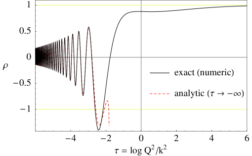
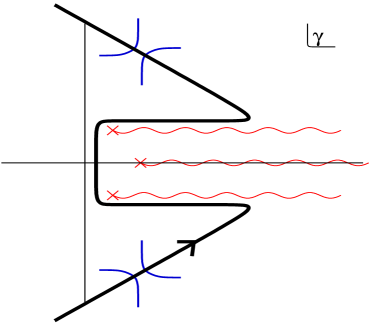
Figure 1: (a) The function $\rho(\tau)$ (solid) and its asymptotic estimates for $\tau\to-\infty$ (dashed). (b) Sketch of the fastest convergence contour in the complex $\gamma$-plane of the integral in Eq. (25) for $\tau\ll-1$, including the cuts and two saddle points that provide the dominant contributions to $\rho$ for very negative $\tau$.

Even if $\Delta(\tau)\equiv\rho(\tau)-\Theta(\tau)$ is in a sense a small quantity — because the first two $\tau$-moments of $\Delta(\tau)$ must vanish — the numerical evaluation of (24) is delicate because of the large oscillations of $\rho$ in the negative $\tau$ region. For $\tau\ll-1$ the fastest convergence contour is shown in Fig. 1.b, where two saddle points $\gamma_{\mathrm{sp}},\gamma_{\mathrm{sp}}^{*}$ of order $\gamma_{\mathrm{sp}}(\tau)\simeq 1+\mathrm{i}\exp\left\{|\tau|+\psi(1)\right\}$ are found. A saddle point evaluation

$$\rho(\tau)|_{\mathrm{sp}}=\sqrt{\frac{2}{\pi}}\;\mathcal{I}m\left\{\frac{\exp\left[c(\tau_{0})+\int_{\tau_{0}}^{\tau}\mathrm{d}\tau^{\prime}\;\gamma_{\mathrm{sp}}(\tau^{\prime})\right]}{{\textstyle\frac{1}{2}}\sqrt{\chi_{0}^{(0)}{}^{\prime}\big{(}\gamma_{\mathrm{sp}}(\tau)\big{)}}}\right\}\;,$$ (26)

provides a good estimate for the contributions from the diagonal parts of the contour, while we integrate numerically the remaining part of the contour. The result (26) is $\tau_{0}$-independent, but the constant of integration $c(\tau_{0})$ is determined numerically, e.g., $c(-3)\simeq-1.18+\mathrm{i}\,2.15$. The function $\rho(\tau)$ is also computed entirely numerically for $\tau\gtrsim-7$.

In order to illustrate the difference between small-$x$ gluon distributions in the $Q_{0}$ and $\overline{\mathrm{MS}}$ factorisation schemes, we consider a toy gluon density obtained by inserting a valence-like inhomogeneous term $f_{0}$ in the RGI equation of [6], as follows

$$f_{0}(x,t)=Ax^{0.5}(1-x)^{5}\delta(t-t_{0})\qquad(e^{t_{0}}\equiv k_{0}^{2}=0.55\;\mathrm{GeV}^{2})\;,$$ (27)

and solving the corresponding evolution for the unintegrated gluon density $f(x,t)\equiv\mathcal{G}(Q^{2},k_{0}^{2};x)$ where $t\equiv\log Q^{2}/\mu^{2}$. The normalisation $A$ is set so that the inhomogeneous term has a momentum sum-rule equal to $1/2$. The solution of the RGI equation approximately maintains the sum-rule for the full resulting gluon, though not exactly because of some higher-twist violations.

We then define the integrated densities

$$xg^{(Q_{0})}(x,Q^{2}) =\int dt^{\prime}\,\Theta(t-t^{\prime})\,f(x,t^{\prime})$$ (28)

$$xg^{(\overline{\mathrm{MS}})}(x,Q^{2}) =\int dt^{\prime}\,\rho(t-t^{\prime})\,f(x,t^{\prime})\;,$$ (29)

which are shown in Fig. 2 in comparison to CTEQ (NLO) and MRST (NNLO) fits for the $\overline{\mathrm{MS}}$ gluon at two scales. Note that we have not attempted to fine-tune the inhomogeneous gluon term to get good agreement at large $x$ since in any case we neglect the quark part of the evolution which is likely to contribute non-negligibly there.

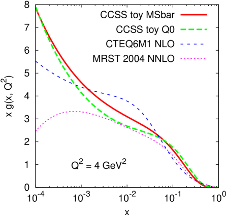
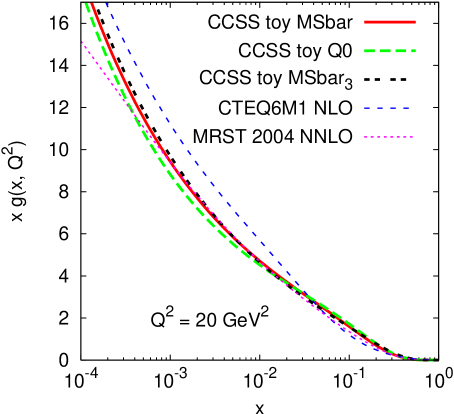
Figure 2: Toy gluon at scales $Q^{2}=4\;\mathrm{GeV}^{2}$ and $20\;\mathrm{GeV}^{2}$ in the $Q_{0}$ and $\overline{\mathrm{MS}}$ schemes, compared to MRST2004 (NNLO) [15] and CTEQ6M1 (NLO) [16]. At the higher $Q^{2}$ value we also show the $\overline{\mathrm{MS}}_{3}$ approximation to the full $\overline{\mathrm{MS}}$ evaluation.

One observes that the difference between the $Q_{0}$ and $\overline{\mathrm{MS}}$ schemes is modest compared to that between the CTEQ and MRST fits and, in particular, there is no tendency for the $\overline{\mathrm{MS}}$ density to go negative. This is despite the violently oscillatory nature of $\rho$, which might have been expected to lead to significant corrections. This can in part be understood from the approximate form of $g^{(\overline{\mathrm{MS}})}$

$$xg^{(\overline{\mathrm{MS}}_{3})}(x,Q^{2})\equiv xg^{(Q_{0})}(x,Q^{2})-\frac{8\zeta(3)}{3}\frac{d^{3}}{dt^{3}}\big{[}xg^{(Q_{0})}(x,Q^{2})\big{]}\;,$$ (30)

which is obtained by expanding the scheme-change in the anomalous dimension variable $\gamma\sim\mathrm{d}/\mathrm{d}t$ to first non-trivial order. We can see that this approximation is pretty good in the small-$x$ region for reasonable values of $\alpha_{\mathrm{s}}$ ($Q^{2}=20\;\mathrm{GeV}^{2}$), corresponding to an effective $\gamma\simeq 0.25$.

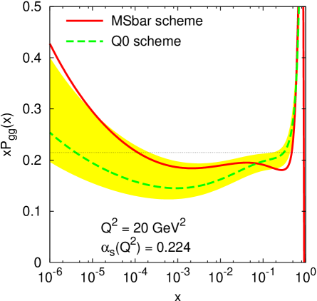
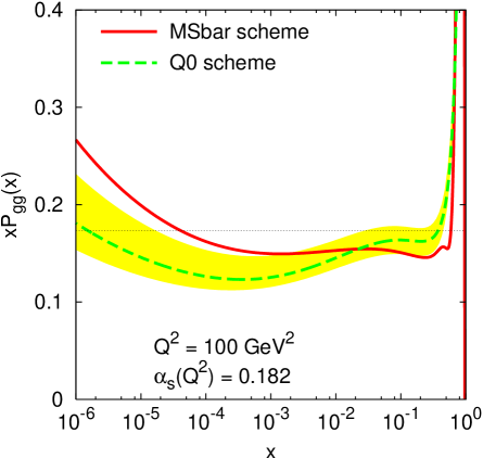
Figure 3: Resummed $P_{gg}$ splitting function in the $Q_{0}$ and $\overline{\mathrm{MS}}$ schemes together with the uncertainty band for the $Q_{0}$ scheme that comes from varying the renormalisation scale for $\alpha_{s}$ by a factor $x_{\mu}$, in the range $1/2<x_{\mu}<2$; shown for two $Q^{2}$ values.

We can also use our usual techniques [26] for extracting the splitting function itself in the $\overline{\mathrm{MS}}$-scheme. The results are shown in Fig. 3, where the $\overline{\mathrm{MS}}$ curve is supposed to be reliable in the small-$x$ region only ($x\lesssim 10^{-1}$), because at finite $x$ the $\omega$-dependence of the scheme change will become important. It appears that the splitting function is more sensitive to the scheme-change than the density itself. At the lower $Q^{2}$ value the difference between the $\overline{\mathrm{MS}}$-scheme and the $Q_{0}$-scheme (with $\mathrm{NLL_{B^{\prime}}}$ resummation) is nearly the same as the renormalisation scale uncertainty and so might not be considered a major effect. Recall however that the scale uncertainty is NNL$x$ whereas the factorisation scheme change is a NL$x$ effect, so that while the renormalisation scale uncertainty decreases quite rapidly as $Q^{2}$ is increased (right-hand plot), the effect of the factorisation scheme change remains non-negligible.

At small $x$, most of the difference between the $\overline{\mathrm{MS}}$ and $Q_{0}$ splitting functions seems to be due to the $\overline{\mathrm{MS}}$ splitting function rising as a larger power of $1/x$. One can check this interpretation by estimating the factorisation-scheme dependence of the asymptotic $x^{-\omega_{c}}$ behaviour, using the $\overline{\mathrm{MS}}_{3}$ approximation. We find

$$\Delta\omega_{c}(t)=\omega_{c}^{\overline{\mathrm{MS}}}-\omega_{c}^{Q_{0}}\simeq-\frac{\mathrm{d}\omega_{c}(t)}{\mathrm{d}t}\frac{8\zeta(3)}{3}\frac{g^{\prime\prime\prime}\big{(}t,\omega_{c}(t)\big{)}}{g^{\prime}\big{(}t,\omega_{c}(t)\big{)}}\simeq 0.029\,,$$ (31)

where the numerical value is given for $Q^{2}=20\;\mathrm{GeV}^{2}$, and is in rough agreement with what is seen in the left-hand plot of Fig. 3.

3 Approximate resummed splitting function for the $\boldsymbol{\overline{\mathrm{MS}}}$ quark

Let us now discuss the inclusion of quarks in the resummed, small-$x$ flavour singlet evolution. Resummation effects will be included via the unintegrated gluon density as discussed before, while the scheme-change to the $\overline{\mathrm{MS}}$-quark will be an (approximate) $\boldsymbol{k}$-factorised form of the one arising at first non-trivial LL$x$ level.

In order to better specify the scheme change, we first recall [18] that the quark density in a physical $Q_{0}$-scheme corresponding to the measuring process $p$ (e.g. $F_{2}$ or $F_{T}$ in DIS) — which we call $p$-scheme — is defined, at NL$x$ level, by $\boldsymbol{k}$-factorisation of some $g\to q\bar{q}$ impact factor $H_{\varepsilon}^{(p)}$, as follows:

$$q_{\varepsilon}^{(p)}(t)\equiv\alpha_{\mu}\int\mathrm{d}^{2+2\varepsilon}\boldsymbol{k}^{\prime}\;H_{\varepsilon}^{(p)}(\boldsymbol{k},\boldsymbol{k}^{\prime}){\mathcal{F}}_{\varepsilon}(\boldsymbol{k}^{\prime})\;.$$ (32)

By then working out this convolution in terms of the eigenvalue function $\mathcal{H}^{(p)}_{\varepsilon}(\gamma)/\gamma(\gamma+\varepsilon)$ of $H_{\varepsilon}^{(p)}$, one directly obtains a NL$x$ resummation formula for the $\varepsilon$-dependent $qg$ anomalous dimension in the $p$-scheme:

$$\left[g_{\varepsilon}^{(Q_{0})}(t)\right]^{-1}\frac{\mathrm{d}}{\mathrm{d}t}q_{\varepsilon}^{(p)}(t)\equiv\gamma_{qg}^{(p)}\big{(}\alpha_{\mathrm{s}}(t),\omega;\varepsilon\big{)}\;,$$ (33)

where, in the $\varepsilon=0$ limit, $\gamma_{qg}^{(p)}=\alpha_{\mathrm{s}}(t)\mathcal{H}^{(p)}_{0}(\gamma_{\mathrm{L}})$ has been obtained in closed form in various cases [18, 20], including sometimes the $\varepsilon$-dependence.

The $\overline{\mathrm{MS}}$-scheme is then related to the $p$-scheme by the transformation

$$q^{(p)}=C_{qq}^{(p)}q^{(\overline{\mathrm{MS}})}+C_{qg}^{(p)}g^{(\overline{\mathrm{MS}})}\;,$$ (34)

where we set $C_{qq}^{(p)}=1$ and $b=0$ at NL$x$ level, so that $\alpha_{\mathrm{s}}(t)=\alpha_{\mu}\mathrm{e}^{\varepsilon t}$. We thus obtain, by the definition (33) and by Eq. (1),

$$\gamma_{qg}^{(p)}(\alpha_{\mathrm{s}},\omega;\varepsilon)R(\alpha_{\mathrm{s}},\omega;\varepsilon) =\left(g_{\varepsilon}^{(\overline{\mathrm{MS}})}\right)^{-1}\frac{\mathrm{d}}{\mathrm{d}t}\left[C_{qg}^{(p)}(\alpha_{\mathrm{s}},\omega;\varepsilon)g_{\varepsilon}^{(\overline{\mathrm{MS}})}\right]+\gamma_{qg}^{(\overline{\mathrm{MS}})}(\alpha_{\mathrm{s}},\omega)$$

$$=\left[\gamma_{\mathrm{L}}\big{(}\frac{\bar{\alpha}_{\mathrm{s}}}{\omega}\big{)}+\varepsilon\hat{D}\right]C_{qg}^{(p)}(\alpha_{\mathrm{s}},\omega;\varepsilon)+\gamma_{qg}^{(\overline{\mathrm{MS}})}(\alpha_{\mathrm{s}},\omega)\;,$$ (35)

where $\hat{D}=\alpha_{\mathrm{s}}\partial/\partial\alpha_{\mathrm{s}}$ and $\gamma_{qg}^{(\overline{\mathrm{MS}})}$ is universal and $\varepsilon$-independent, so that the process dependence of $\gamma_{qg}^{(p)}$ is carried by the perturbative, scheme-changing coefficient $C_{qg}^{(p)}$.

The coefficient $C_{qg}^{(p)}$ in Eq. (35) can be formally eliminated by promoting $\varepsilon$ to be an operator in $\alpha_{\mathrm{s}}$-space, as follows:

$$\varepsilon=-\gamma_{\mathrm{L}}\big{(}\frac{\bar{\alpha}_{\mathrm{s}}}{\omega}\big{)}\hat{D}^{-1}\;,$$ (36)

so that the square bracket in Eq. (35) in front of $C_{qg}^{(p)}$ just vanishes (this procedure is rigorously justified in [20]). That implies that the l.h.s. of Eq. (35) and $\mathcal{H}^{(p)}_{\varepsilon}(\gamma)$ are to be evaluated at values of $\varepsilon\sim\gamma_{\mathrm{L}}=\mathcal{O}\left(\alpha_{\mathrm{s}}/\omega\right)$ which modifies $\gamma_{qg}^{(\overline{\mathrm{MS}})}-\gamma_{qg}^{(p)}$ at relative LL$x$ level. Therefore, even if $\gamma_{qg}^{(\overline{\mathrm{MS}})}$ is by itself a NL$x$ quantity, the subtraction of the coefficient part in Eq. (35) affects the scheme change at relative leading order, contrary to the gluon case of Eqs. (13) and (22).

The replacement (36) was used in [20] in order to get an “exact” expression of $\gamma_{qg}^{(\overline{\mathrm{MS}})}$ at NL$x$ level (that is, resumming the series of next-to-leading $\omega$-singularities $\sim\alpha_{\mathrm{s}}(t)[\alpha_{\mathrm{s}}(t)/\omega]^{n}$). The main observation is that, by expanding $\mathcal{H}^{(p)}_{\varepsilon}(\gamma)$ in the $\gamma$ variable around $\gamma=-\varepsilon$ with coefficients $\mathcal{H}^{(p)}_{n}(\varepsilon)$, and by converting Eq. (32) to $\gamma$-space, we obtain

$$\frac{\mathrm{d}}{\mathrm{d}t}q^{(p)}_{\varepsilon}(t) =\alpha_{\mathrm{s}}(t)\int\mathrm{d}\gamma\;\mathrm{e}^{\gamma t}\mathcal{H}^{(p)}_{\varepsilon}(\gamma)\tilde{g}_{\varepsilon}(\gamma,\omega)$$

$$=\left(\mathcal{H}(\varepsilon)+\sum_{n=1}^{\infty}\mathcal{H}^{(p)}_{n}(\varepsilon)\frac{\mathrm{d}^{n}}{\mathrm{d}t^{n}}\right)\left(\alpha_{\mathrm{s}}(t)R\Big{(}\frac{\bar{\alpha}_{\mathrm{s}}}{\omega},\varepsilon\Big{)}g_{\varepsilon}^{(\overline{\mathrm{MS}})}(t,\omega)\right)\;,$$ (37)

where $\tilde{g}_{\varepsilon}(\gamma,\omega)$ is the Fourier transform of $g_{\varepsilon}^{(\overline{\mathrm{MS}})}(t,\omega)$ and $\mathcal{H}(\varepsilon)\equiv\mathcal{H}^{(p)}_{\varepsilon}(-\varepsilon)$ turns out to be the universal function

$$\mathcal{H}(\varepsilon)=\left[\frac{T_{R}}{2\pi}\,\frac{2}{3}\,\frac{1+\varepsilon}{(1+2\varepsilon)(1+\frac{2}{3}\varepsilon)}\right]\left[\frac{\mathrm{e}^{\varepsilon\psi(1)}\Gamma^{2}(1+\varepsilon)\Gamma(1-\varepsilon)}{\Gamma(1+2\varepsilon)}\right]\equiv\mathcal{H}^{\mathrm{rat}}(\varepsilon)\mathcal{H}^{\mathrm{tran}}(\varepsilon)\;,$$ (38)

which we factorise into parts with rational and transcendental coefficients. Note that the universality of $\mathcal{H}(\varepsilon)$, which is proportional to the residue of the characteristic function $\mathcal{H}^{(p)}_{\varepsilon}(\gamma)/\gamma(\gamma+\varepsilon)$ at the collinear pole $\gamma=-\varepsilon$, is due to the interesting fact that one can define [18] a universal [20], off-shell $g(\boldsymbol{k})\to q(\boldsymbol{l})$ splitting function in the collinear limit $\boldsymbol{k}^{2}\sim\boldsymbol{l}^{2}\ll Q^{2}$, for any ratio $\boldsymbol{k}^{2}/\boldsymbol{l}^{2}$ of the corresponding virtualities.

We then realise from Eq. (37) that the terms in the r.h.s. with at least one derivative $\mathrm{d}/\mathrm{d}t$ are of coefficient type, and vanish by the replacement (36). The remaining one, proportional to $\mathcal{H}(\varepsilon)$, is universal and, by (36), yields the NL$x$ result [20]

$$\gamma_{qg}^{(\overline{\mathrm{MS}})}\big{(}\alpha_{\mathrm{s}}(t),\omega\big{)}=\alpha_{\mathrm{s}}(t)\mathcal{H}^{\mathrm{rat}}\bigg{(}-\gamma_{\mathrm{L}}\Big{(}\frac{\bar{\alpha}_{\mathrm{s}}(t)}{\omega}\Big{)}\frac{1}{1+\hat{D}}\bigg{)}\sum_{n=0}^{\infty}\left(\gamma_{\mathrm{L}}\Big{(}\frac{\bar{\alpha}_{\mathrm{s}}(t)}{\omega}\Big{)}\frac{1}{1+\hat{D}}\right)^{n}R_{n}\Big{(}\frac{\bar{\alpha}_{\mathrm{s}}(t)}{\omega}\Big{)}\;,$$ (39)

where we have factorised $\alpha_{\mathrm{s}}(t)$ by the commutator $[\hat{D},\alpha_{\mathrm{s}}]=\alpha_{\mathrm{s}}$ and we have defined the quantity

$$\mathcal{H}^{\mathrm{tran}}(\varepsilon)R\Big{(}\frac{\bar{\alpha}_{\mathrm{s}}}{\omega},\varepsilon\Big{)}=\sum_{n=0}^{\infty}(-\varepsilon)^{n}R_{n}\Big{(}\frac{\bar{\alpha}_{\mathrm{s}}}{\omega}\Big{)}\;,$$ (40)

which has transcendental coefficients and differs from unity by terms of order $(\gamma_{\mathrm{L}})^{3}$ or higher, in the $\varepsilon\sim\gamma_{\mathrm{L}}$ region [18, 20].

The complicated expression (39) has been evaluated iteratively [18], but not resummed in closed form. However, it can be drastically simplified in the $\boldsymbol{k}$-factorised framework by neglecting the transcendental corrections $\mathcal{O}\left(\gamma^{3}\right)$, on the ground that the resummed anomalous dimension is small. In fact, by setting $R=\mathcal{H}^{\mathrm{tran}}=1$ and $\gamma_{\mathrm{L}}=\bar{\alpha}_{\mathrm{s}}/\omega$, Eq. (39) reduces to the expression

$$\gamma_{qg}^{(\overline{\mathrm{MS}})}\simeq\alpha_{\mathrm{s}}(t)\mathcal{H}^{\mathrm{rat}}\Big{(}-\frac{\bar{\alpha}_{\mathrm{s}}}{\omega}\frac{1}{1+\hat{D}}\Big{)}\cdot 1=\alpha_{\mathrm{s}}(t)\sum_{n}\frac{\mathcal{H}^{\mathrm{rat}}_{n}}{n!}\left(\frac{\bar{\alpha}_{\mathrm{s}}}{\omega}\right)^{n}\;,$$ (41)

which is just the Borel transform of

$$\mathcal{H}^{\mathrm{rat}}(\varepsilon)=\sum_{n}\mathcal{H}^{\mathrm{rat}}_{n}\,(-\varepsilon)^{n}=\frac{T_{R}}{4\pi}\left[\frac{1}{1+2\varepsilon}+\frac{1}{3}\,\frac{1}{1+\frac{2}{3}\varepsilon}\right]\;.$$ (42)

Since $\mathcal{H}^{\mathrm{rat}}_{n}=\frac{T_{R}}{4\pi}[2^{n}+\frac{1}{3}(\frac{2}{3})^{n}]$ we obtain from (41) what we call the “rational” approximation NL$x|_{\mathrm{rat}}$ (first derived in [18])

$$\left.\gamma_{qg}^{(\overline{\mathrm{MS}})}\right|_{\mathrm{rat}}\simeq\frac{\alpha_{\mathrm{s}}(t)T_{R}}{4\pi}\left(\mathrm{e}^{2\frac{\bar{\alpha}_{\mathrm{s}}}{\omega}}+\frac{1}{3}\mathrm{e}^{\frac{2}{3}\frac{\bar{\alpha}_{\mathrm{s}}}{\omega}}\right)\;.$$ (43)

This result can be further interpreted in $\boldsymbol{k}$-factorised form

$$\frac{\mathrm{d}q_{\mathrm{rat}}^{(\overline{\mathrm{MS}})}}{\mathrm{d}t}=H^{(\overline{\mathrm{MS}})}_{\mathrm{rat}}\otimes f\;,$$ (44)

by using the characteristic function

$$\mathcal{H}^{(\overline{\mathrm{MS}})}_{\mathrm{rat}}(\gamma)=\frac{\alpha_{\mathrm{s}}T_{R}}{4\pi}\frac{1}{\gamma}\left(\mathrm{e}^{2\gamma}+\frac{1}{3}\mathrm{e}^{\frac{2}{3}\gamma}\right)\;,$$ (45)

which yields the result in Eq. (43) at the LL saddle point.

Finally, since the exponentials in (45) generate translations in $t$, our rough estimate of the resummed $P_{qg}$ is provided by the simple formula

$$\frac{\mathrm{d}}{\mathrm{d}t}q_{\mathrm{rat}}^{(\overline{\mathrm{MS}})}(t,x) =\frac{\alpha_{\mathrm{s}}(t)T_{R}}{4\pi}\left[g\big{(}t+2,x\big{)}+\frac{1}{3}g\big{(}t+\frac{2}{3},x\big{)}\right]$$ (46a)

$$=\int_{x}^{1}\frac{\mathrm{d}z}{z}\;P_{qg}^{(\overline{\mathrm{MS}})}\big{(}\alpha_{\mathrm{s}}(t),z\big{)}g\big{(}t,\frac{x}{z}\big{)}\;.$$ (46b)

By replacing in Eq. (46a) the resummed gluon density [6] and by performing the necessary deconvolution [26] we obtain the results in Fig. 4, compared to NLO and NL$x$ [18] results.

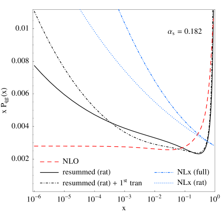
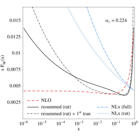
Figure 4: The $\overline{\mathrm{MS}}$ $g\to q$ splitting function for two values of $\alpha_{\mathrm{s}}$ and in various approximations: at two-loop [dashed], the RGI resummed rational one in Eq. (46) [solid] and with the addition of the first transcendental correction [dash-dotted], the rational NL$x$ approximation [dotted] and the complete NL$x$ one [dash-dot-dotted]

A proper comparison of the curves in Fig. 4 can be made only in the small-$x$ region $x\lesssim 10^{-1}$ because Eqs. (39) and (46) do not include the finite-$x$ perturbative terms. We then notice that small-$x$ resummation effects in $q_{\mathrm{rat}}^{(\overline{\mathrm{MS}})}$ are sizeable even around $x\sim 10^{-3}$ and somewhat larger than the gluonic ones. They are anyway much smaller than the corresponding ones of the NL$x$ result, thus showing that the resummed anomalous dimension variable is pretty small, as already noticed in the gluon case. We can also check how good the “rational” resummation is, by calculating the effect of the first $\mathcal{O}\left(\gamma^{3}\right)$ transcendental correction, which is also shown in Fig. 4. It appears that the difference is indeed not large and anyway much smaller than the difference between the results of NL$x|_{\mathrm{rat}}$ in Eq. (43) and NL$x$ [18], both shown in Fig. 4.

To sum up, we have proposed here a $\boldsymbol{k}$-factorised form of the $Q_{0}\to\overline{\mathrm{MS}}$ scheme-change (Eqs. (23) and (44)) which allows a convergent leading log hierarchy, because of the smoothness of the resummed anomalous dimension. Applying the leading scheme change to the gluon density and — in an approximate way — to the quark density we have provided predictions for the $gg$ and $qg$ splitting functions in the $\overline{\mathrm{MS}}$-scheme and for the corresponding densities.

We find that the gluon density itself is rather insensitive to the scheme change, while its splitting function is somewhat sensitive. Resummation effects for the $\overline{\mathrm{MS}}$ quark are more important, but anyway much smaller than those at NL$x$ level. We are thus confident that the scheme change can be calculated in a reliable way in a fully resummed approach as well.

References

[1]
V.N. Gribov and L.N. Lipatov, Sov. J. Nucl. Phys. 15 (1972) 438;
G. Altarelli and G. Parisi, Nucl. Phys. B 126 (1977) 298;
Yu.L. Dokshitzer, Sov. Phys. JETP 46 (1977) 641.
[2]
S. Moch, J. A. M. Vermaseren and A. Vogt,
Nucl. Phys. B 688 (2004) 101;
Nucl. Phys. B 691 (2004) 129.
[3] G.P. Salam, JHEP 9807 (1998) 019.
[4] M. Ciafaloni and D. Colferai, Phys. Lett. B 452 (1999) 372.
[5] M. Ciafaloni, D. Colferai and G.P. Salam,
Phys. Rev. D 60 (1999) 114036.
[6]
M. Ciafaloni, D. Colferai, G.P. Salam and A.M. Staśto,
Phys. Lett. B 576 (2003) 143;
Phys. Rev. D 68 (2003) 114003.
[22]
V. S. Fadin and L. N. Lipatov,
Phys. Lett. B 429 (1998) 127.
[23]
G. Camici and M. Ciafaloni,
Phys. Lett. B 412 (1997) 396
[Erratum-ibid. B 417 (1998) 390];
Phys. Lett. B 430 (1998) 349.
[24]
V. S. Fadin and L. N. Lipatov,
JETP Lett. 49 (1989) 352
[Yad. Fiz. 50 (1989 SJNCA,50,712.1989) 1141];
Nucl. Phys. B 406 (1993) 259;
Nucl. Phys. B 477 (1996) 767.
V. S. Fadin, R. Fiore and A. Quartarolo,
Phys. Rev. D 50 (1994) 2265;
Phys. Rev. D 50 (1994) 5893.
V. S. Fadin, R. Fiore and M. I. Kotsky,
Phys. Lett. B 359 (1995) 181;
Phys. Lett. B 387 (1996) 593;
Phys. Lett. B 389 (1996) 737.
V. S. Fadin, M. I. Kotsky and L. N. Lipatov,
BUDKER-INP-1996-92, arXiv:hep-ph/9704267.
V. Del Duca,
Phys. Rev. D 54 (1996) 989;
Phys. Rev. D 54 (1996) 4474.
V.S. Fadin, R. Fiore, A. Flachi and M.I. Kotsky,
Phys. Lett. B 422 (1998) 287.
[25]
S. Catani, M. Ciafaloni and F. Hautmann,
Phys. Lett. B 242 (1990) 97;
Nucl. Phys. B 366 (1991) 135.
G. Camici and M. Ciafaloni, Phys. Lett. B 386 (1996) 341;
Nucl. Phys. B 496 (1997) 305
[Erratum-ibid. B 607 (2001) 431].
[26]
M. Ciafaloni, D. Colferai and G. P. Salam,
JHEP 0007 (2000) 054.