Two-Photon Effects in Lepton-AntiLepton Pair Photoproduction from a Nucleon Target using Real Photons

Abstract

We consider the production of a lepton-antilepton pair by real photons off a hadronic target. The interference of one and two photon exchange amplitudes leads to a charge asymmetry term that may be calculated explicitly in the large-$t$ limit in terms of hadronic distribution amplitudes. A rather compact expression emerges for the leading order asymmetry at fixed angle in the centre-of-mass of the lepton pair. The magnitude appears sizeable and is approximately independent of the pair mass in the asymptotic limit.

Measurement of the nucleon’s electric and magnetic form factors has traditionally been based upon the well-known Rosenbluth formula[1] which assumes that scattering occurs through the exchange of a single photon. A recent extraction of $G_{E}^{p}/G_{M}^{p}$ in the $Q^{2}$ range from 0.5 to 5.6 $GeV^{2}$ has used the polarization-transfer technique exploited at Jefferson Laboratory[2]. This method, which does not use the Rosenbluth separation, revealed a large discrepancy with previously published form factors. Subsequently, a close scrutiny was made of two-photon exchange effects in elastic electron-proton scattering. In this process a virtual photon knocks the incident proton into an excited state, and a second one de-excites it back into the ground state. Both photons may be hard, and hence they probe nucleon structure. The effects were found to exist at a few percent level and are capable of resolving the observed discrepancy[3]. Model dependence is inevitable. Chen et al. [4] have also calculated the two-photon exchange contribution and related it to the generalized parton distributions[5] that occur in various other hard processes as well. A clear exposition of experimental techniques and two-photon physics may be found in a review by Wright and Jager[6].

In this paper, we shall consider two-photon effects in the production of a lepton-antilepton pair from a hadronic target by real photons (see Fig. 1) at high centre of mass energy $s$.

Figure 1: Exclusive photoproduction of a lepton pair off a proton target.

The process predominantly occurs through the exchange of one photon,with a two-photon admixture. Both amplitudes are for the same final state and so interfere with one another. These exchanges come from diagrams with opposite charge conjugation [7]. This fact enables one to isolate the interference term by counting the difference in the number of produced antileptons and leptons. In the limit of large momentum transfer $t$, they can be explicitly computed from the leading Fock-state in terms of lowest order hadronic distribution amplitudes. We find a rather compact expression for the leading order asymmetry at fixed angle in the centre-of-mass of the lepton pair. The inputs to this calculation, apart from the hadron distribution amplitudes, are experimentally determined hadronic form factors at sufficiently large $t$. We note that Berger, Diehl, and Pire had analyzed and estimated exclusive lepton pair photoproduction (at small $t$) as a means of studying generalized parton distributions in the nucleon[8]. Exclusive electroproduction of J/psi mesons (which then decay into lepton pairs) has been studied at HERA[9] for fairly small $Q^{2}$ values.

Before considering the more complex case of the proton, we shall first consider a pion target. It is convenient to work in the rest frame of the produced lepton-antilepton pair. The mass of the quarks, and of the hadronic target, have been ignored in this preliminary calculation, i.e. $P^{2}=P^{\,\prime\,2}=0$ where $P^{\mu}$ and $P^{\,\prime\mu\,}$ are the momenta of the initial and final hadron. The squared invariant mass of the produced leptons (also assumed massless) is $M^{2}$. This may be selected at will and should be chosen far away from a resonance. Simple expressions emerge only for $s>>-t,M^{2}>>\Lambda_{QCD}^{2}$ where $t$ is defined, as usual, from $t=(P-P^{\,\prime})^{2}.$ It is negative in the physical region. The incoming real photon ($q^{2}=0$) is taken along the $z$-axis, and the $x-z$ scattering plane is defined by the incoming vectors $q^{\mu}$ and $P^{\mu}$outgoing, elastically scattered, hadron is in the $x-z$ plane. The sum of the lepton-antilepton momentum vectors is $K^{\mu}=l^{\mu}+l^{{}^{\prime}\mu}$. A convenient parametrization of the scattering kinematics is then provided by,

$$q^{\mu} = (\omega,0,0,\omega),$$ (1)

$$P^{\mu} = (\epsilon,\epsilon\sin\psi,0,\epsilon\cos\psi),$$ (2)

$$P^{\,\prime\,\mu} = (\epsilon+\omega-M,\epsilon\sin\psi,0,\omega+\epsilon\cos\psi),$$ (3)

$$K^{\mu} = (M,0,0,0),$$ (4)

where the incoming hadron energy $\epsilon$, incoming photon energy $\omega$, and angle $\psi$ are,

$$\epsilon = \frac{s+t}{2M},$$ (5)

$$\omega = \frac{M^{2}-t}{2M},$$ (6)

$$\cos\psi = 1-\frac{s}{2\omega\epsilon}.$$ (7)

The outgoing lepton and antilepton, also taken to be massless, have spinors $\overline{u}(l)$ and v$(l^{{}^{\,\prime}}).$ The lepton and anti-lepton momentum vectors are,

$$l^{\,\mu} = \frac{M}{2}(1,\sin\theta\cos\phi,\sin\theta\sin\phi,\cos\theta),$$ (8)

$$l^{{}^{\prime}\,\mu} = \frac{M}{2}(1,-\sin\theta\cos\phi,-\sin\theta\sin\phi,-\cos\theta).$$ (9)

The azimuthal angle $\phi$ is measured relative to the plane formed by $\overrightarrow{P}$ and $\overrightarrow{q}$ (which defines the z-axis and hence $\theta$). In the centre-of-mass frame used here $\overrightarrow{P}^{\,\prime}$ also lies in this plane. By angular momentum conservation, the two massless leptons have opposite helicities. Since we shall work at the amplitude level, we need simple, covariant expressions for the matrix v$(l^{{}^{\,\prime}})\overline{u}(l)$ in the helicity basis. The method developed by Vega and Wudka[10] is especially convenient when used in the cm frame:

$$\text{v}_{\downarrow}(l^{{}^{\,\prime}})\overline{u}_{\uparrow}(l) = -\frac{M}{4}\eta_{+}\!\!\!\!\!\!/\;\;+\frac{M}{4}\eta_{+}\!\!\!\!\!\!/\,\;\gamma_{5},$$ (10)

$$\text{v}_{\uparrow}(l^{{}^{\,\prime}})\overline{u}_{\downarrow}(l) = -\frac{M}{4}\eta_{-}\!\!\!\!\!\!/\;\;-\frac{M}{4}\eta_{-}\!\!\!\!\!\!/\,\;\gamma_{5}.$$ (11)

since it will not enter the cross-sections. The auxiliary vector $\eta_{\pm}^{\mu}$ is defined as,

$$\eta_{\pm}^{\mu}=(0,\cos\theta\cos\phi\pm i\sin\phi,\cos\theta\cos\phi\mp i\cos\phi,-\sin\theta).$$ (12)

Here $\pm$ refers to the lepton helicity. $\eta^{\mu}$ satisfies,

$$\eta_{-} = \eta_{+}^{\ast},$$ (13)

$$\eta_{+}\cdot\eta_{+} = \eta_{-}\cdot\eta_{-}=0,$$ (14)

$$\eta_{\pm}\cdot l = \eta_{\pm}\cdot l^{{}^{\,\prime}}=0.$$ (15)

Consider now lepton pair production from a pion via the form factor diagram (Fig.2). This, together with its crossed counterpart, is easily calculated in the large $s$ limit.

With the pion factor normalized such that $F_{\pi}(0)=1$, the amplitude for producing a positive helicity lepton from a positive helicity real photon is,

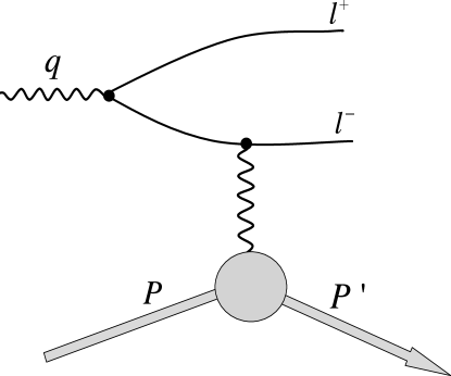
Figure 2: Form-factor contribution to lepton pair production at lowest order.

$$A_{1}^{\uparrow\uparrow} \equiv A_{1}(\theta,\phi,\gamma^{\uparrow},l^{\uparrow},\bar{l}^{\downarrow})$$

$$= -i\sqrt{2}e^{3}\frac{s}{M^{3}\sqrt{\rho}(1+\rho)^{2}}e^{-i\theta}\left[i\sqrt{\rho}(e^{i\theta}-1)+e^{i\phi}(e^{i\theta}+1)\right]^{2}\csc\theta\;F_{\pi}(t)$$

For convenience we have defined the dimensionless momentum transfer,

$$\rho=-\frac{t}{M^{2}}.$$ (17)

By examining the $\gamma$-matrix structure, the other helicity amplitudes are easily obtained from,

$$A_{1}^{\downarrow\uparrow} \equiv A_{1}(\theta,\phi,\gamma^{\downarrow},l^{\uparrow},l^{\prime\downarrow})=A_{1}(\theta+\pi,-\phi,\gamma^{\uparrow},l^{\uparrow},l^{\prime\downarrow}),$$ (18)

$$A_{1}^{\uparrow\downarrow} \equiv A_{1}(\theta,\phi,\gamma^{\uparrow},l^{\downarrow},l^{\prime\uparrow})=A_{1}(\theta+\pi,\phi,\gamma^{\uparrow},l^{\uparrow},l^{\prime\downarrow}),$$ (19)

$$A_{1}^{\downarrow\downarrow} \equiv A_{1}(\theta,\phi,\gamma^{\downarrow},l^{\downarrow},l^{\prime\uparrow})=A_{1}(\theta,-\phi,\gamma^{\uparrow},l^{\uparrow},l^{\prime\downarrow}).$$ (20)

For momentum transfers much higher than the invariant mass of the produced lepton pair

$$A_{1}^{\uparrow\uparrow}\rightarrow-i\frac{\sqrt{8}e^{3}}{(-t)^{3/2}}s\tan\frac{\theta}{2}F_{\pi}(t)\;\;\;\;(s>>-t>>M^{2}).$$ (21)

Note that the $\phi$ dependence entirely disappears in this limit. The singular behaviour for $\theta\rightarrow 0$ comes from the lepton propagator in Fig.2 and disappears upon including the lepton mass. However, for purposes of comparing with the other amplitudes to be computed below, where including the mass would make the formulae less transparent, this mass will be kept at zero in this preliminary calculation.

The squared amplitude from Fig.2, summed over lepton polarizations, and averaged over photon polarizations, is:

$$\sum_{\gamma,s}\left|A_{1}^{\gamma s}\right|^{2}=\frac{32s^{2}e^{6}F_{\pi}^{2}(t)}{M^{6}\rho(1+\rho)^{4}}\sum_{n=0}^{2}a_{n}\cos n\phi.$$ (22)

The coefficients $a_{n}$ are ,

$$a_{0} = -(\rho^{2}-4\rho+1)+2(\rho^{2}+1)\csc^{2}\theta,$$ (23)

$$a_{1} = 4\sqrt{\rho}(\rho-1)\cot\theta,$$ (24)

$$a_{2} = 2\rho.$$ (25)

Under spatial inversion (i.e. $\theta\rightarrow\theta+\pi$ and $\phi\rightarrow\phi$ ) the outgoing lepton and anti-lepton are exchanged. But $\frac{d\sigma}{dt}\;$, computed from Eq. 22 suffers no change. In other words the charge asymmetry at leading order is zero.

A fermion line attached to three vector vertices has the opposite charge conjugation properties relative to the same line with two vertices. We shall use this property in an essential way. So, now consider scattering into the same final state but through the exchange of two photons. The three photon vertices may be connected to the $l^{-}l^{+}$ line in six different ways, two of which have been shown in Fig.3.

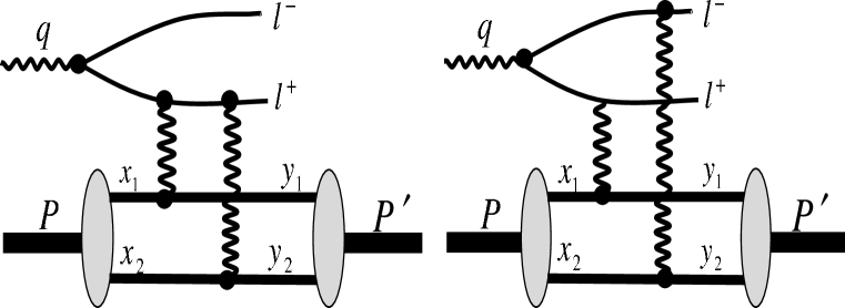
Figure 3: Typical two-photon contributions to lepton photoproduction from a pion target.

In general, the scattering from any hadronic state is extremely complicated and, in the language of Fock states, involves an infinite number of proton wavefunction components. However, in the large-$t$ limit, all higher components beyond the minimal one are strongly suppressed in a purely exclusive process. The reason is straightforward: every quark and gluon present in the initial state must be “turned around” and its momentum components redirected into the final state. This simple fact allows for calculation of hadronic form-factors[13], as well as generalized parton distributions[14], etc.

In the calculation reported below we assume that large enough values of $t$ can be selected for the minimal 2-quark component of the pion to dominate the scattering. Integrating over the transverse momentum of quarks, one may then approximately represent the pion state by,

$$|\pi^{+},P\rangle = \int\frac{\left[dx\right]}{\sqrt{4x_{1}x_{2}}}\Phi(x_{1},x_{2})\frac{1}{\sqrt{3}}\left\{u_{a\uparrow}^{\dagger}(x_{1})\overline{d}_{a\downarrow}^{\dagger}(x_{2})-u_{a\downarrow}^{\dagger}(x_{1})\overline{d}_{a\uparrow}^{\dagger}(x_{2})\right\}|0\rangle,$$

Where the integration measure is,

$$\left[dx\right]=dx_{1}dx_{2}\delta(1-x_{1}-x_{2}).$$ (27)

Here $a=1,2,3$ denotes colour. Asymptotically, as is well known, $\phi_{\pi}(x)$ approaches $f_{\pi}\sqrt{6}x(1-x).$

The calculation of diagrams in Fig.3 is straightforward. Typically one has a denominator that, expanded out in the large $s$ limit, looks like,

$$\frac{1}{s(x_{1}-y_{1})\left[1+\rho+2\sqrt{\rho}\cos\phi\sin\theta+(\rho-1)\cos\theta\right]+i\epsilon}.$$

This is singular at $x_{1}=y_{1}$, and so has a principal part in addition to an imaginary (delta function) piece. The principal parts cancel when taking the sum of all six diagrams for the upper diagrams. The numerator is of $O(s^{2}),$ and so the overall contribution is proportional to $s$.

After a tedious calculation, the amplitude for producing a positive helicity lepton from a positive helicity real photon via two-photon exchange reads,

$$A_{2}^{\uparrow\uparrow} \equiv A_{2}^{\gamma\pi\rightarrow\pi l^{-}l^{+}}(\theta,\phi)$$ (28)

$$= -\frac{2i\sqrt{2}\pi e_{u}e_{d}e^{3}s\text{ }}{M^{5}\rho^{3/2}(1+\rho)^{2}}e^{-i\theta}(\cos\theta+e^{-i\phi}\frac{M}{\sqrt{-t}}\sin\theta)\left[i\sqrt{\rho}(e^{i\theta}-1)+e^{i\phi}(e^{i\theta}+1)\right]^{2}\times$$

$$\;\int\left[dx\right]\left[dy\right]\frac{\Phi(x_{1},x_{2})\Phi(y_{1},y_{2})\delta(y_{1}-x_{1})}{x_{1}\overline{x}_{1}\left[x_{1}\overline{x}_{1}+\Lambda\right]}.$$

In the above, $\overline{x}_{1}=1-x_{1}$ and the integrand depends upon $\theta$ and $\phi:$

$$\Lambda=\frac{e^{-i\phi}}{4\sqrt{\rho}}\sin 2\theta-\frac{1}{4}(1-\frac{e^{-i2\phi}}{\rho})\sin^{2}\theta.$$ (29)

The other amplitudes can be expressed in terms of $A_{2}^{\uparrow\uparrow}:$

$$A_{2}^{\uparrow\downarrow} \equiv A_{2}(\theta,\phi,\gamma^{\uparrow},l^{\downarrow},\bar{l}^{\uparrow})=-A_{2}(\theta+\pi,\phi,\gamma^{\uparrow},l^{\uparrow},\bar{l}^{\downarrow}),$$ (30)

$$A_{2}^{\downarrow\uparrow} \equiv A_{2}(\theta,\phi,\gamma^{\downarrow},l^{\uparrow},\bar{l}^{\downarrow})=-A_{2}(\theta+\pi,-\phi,\gamma^{\uparrow},l^{\uparrow},\bar{l}^{\downarrow}),$$ (31)

$$A_{2}^{\downarrow\downarrow} \equiv A_{2}(\theta,\phi,\gamma^{\downarrow},l^{\downarrow},\bar{l}^{\uparrow})=A_{2}(\theta,-\phi,\gamma^{\uparrow},l^{\uparrow},\bar{l}^{\downarrow}).$$ (32)

The negative signs in the above amplitudes will be responsible for the charge asymmetry in the crossection, as we shall see shortly. But first, let us remark on the apparent problem in the integral,

$$\int\left[dx\right]\left[dy\right]\frac{\Phi(x_{1},x_{2})\Phi(y_{1},y_{2})\delta(y_{1}-x_{1})}{x_{1}\overline{x_{1}}\left[x_{1}\overline{x_{1}}+\Lambda\right]}.$$ (33)

For $\phi=0$ the integrand is real and has a singularity inside the integration range. However, reinstating the lepton mass removes the singularity by introducing a term of order $m^{2}/M^{2}$. This still leaves a very strong $\phi$ dependence, thereby distinguishing the two-photon exchange term from that with a single photon. A proper calculation must, of course, include lepton masses. One might wonder about other diagrams, also of $O(e^{3}),$ such as those in Fig.4. However, these can be shown to be of $O(1/s)$.

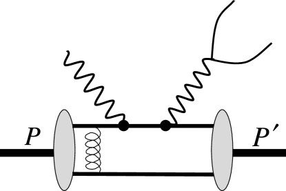
Figure 4: A typical diagram for lepton pairproduction from a single quark in the target. The sum of all such diagrams is suppressed in the large - s limit for real photons.

Now consider the interference term in $\left|A_{1}+A_{2}\right|^{2}$,

$$\Theta(\theta,\phi)=\frac{\sum_{\gamma,s}(A_{1}^{\gamma s}A_{2}^{\ast\gamma s}+A_{1}^{\ast\gamma s}A_{2}^{\gamma s})}{\sum_{\gamma,s}\left|A_{1}^{\gamma s}\right|^{2}}.$$ (34)

After simplication, this becomes,

$$\Theta(\theta,\phi) = \frac{16\pi^{2}e_{u}e_{d}\alpha_{e}}{M^{2}\rho F_{\pi}(t)}(\cos\theta+e^{-i\phi}\frac{1}{\sqrt{\rho}}\sin\theta)$$

$$\times\int\left[dx\right]\left[dy\right]\frac{\Phi(x_{1},x_{2})\Phi(y_{1},y_{2})\delta(y_{1}-x_{1})}{x\overline{x}\left(x\overline{x}+\Lambda\right)}+cc,$$

$$= \frac{16\pi^{2}e_{u}e_{d}\alpha_{e}}{M^{2}\rho F_{\pi}(t)}(\cos\theta+e^{-i\phi}\frac{1}{\sqrt{\rho}}\sin\theta)\int_{0}^{1}dx\frac{\Phi^{2}(x)}{x\overline{x}\left(x\overline{x}+\Lambda\right)}+cc.$$

In the above, $\overline{x}=1-x=1-x_{1}$ and $e_{u}=2/3$, $e_{d}=-1/3$. We define the charge asymmetry as:

$$\Xi(\theta,\phi)=\Theta(\theta+\pi,\phi)-\Theta(\theta,\phi)=-2\Theta(\theta,\phi).$$ (36)

Obviously $\Xi(\theta,\phi)=-\Xi(\theta+\pi,\phi)$. This quantity is proportional to the difference in count rates between antileptons and leptons. As is apparent from the definition of $\Lambda$, the integral over $x$ asymptotically goes to a constant, finite value as $\rho\rightarrow\infty.$ A leading order calculation[13],[15] for the pion form factor gives $(-t)F_{\pi}=12f_{\pi}^{\;2}\pi C_{F}\alpha_{S}$ at large $t$ or, equivalently, $\rho F_{\pi}=12(f_{\pi}^{\;2}/M^{2})\pi C_{F}\alpha_{S}$. Note that $M$, the lepton pair invariant mass, has disappeared from the final formula for $\Xi.$ In Fig.5, $\Xi$ is plotted as a function of $\rho$ for fixed angles. Note that we have assumed collinear quarks and so the formula is valid only for $M$ greater than the typical $k_{T}$ of quarks inside the pion.

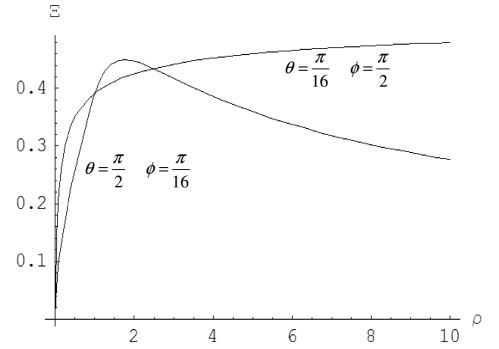
Figure 5: Lepton pair asymmetry from a pion target.

With the above case for the pion as a warm-up, we now proceed to lepton pair production from a 3-quark target. For calculational purposes, it is useful to introduce a 4-vector for the scattered hadron[10],

$$\xi^{\mu} = (0,\cos\psi,-i,-\sin\psi),$$ (37)

$$P\cdot\xi = 0,$$ (38)

in terms of which the proton spinor matrix can be expressed as,

$$u_{\uparrow}(P)\overline{u}_{\uparrow}(P^{\,\prime})=\frac{\gamma_{5}\,\xi\!\!/\,P\!\!\!\!/\,\,P^{{}^{\,\prime}}\!\!\!\!\!\!/}{2\sqrt{2P\cdot P^{\,\prime}}}.$$ (39)

The form-factor contribution to lepton photoproduction off a proton is identical to that from a pion in the limit where the spin-flip term (Pauli form factor) is set to zero. Indeed for massless quarks and no transverse momentum, this is strictly true. The minimal state of the proton is,

$$|P_{\uparrow}\rangle=\int\frac{\left[dx\right]}{2\sqrt{24x_{1}x_{2}x_{3}}}\Phi(x_{1},x_{2},x_{3})\frac{\varepsilon^{abc}}{\sqrt{6}}u_{a\uparrow}^{\dagger}(x_{1})\left\{u_{b\downarrow}^{\dagger}(x_{2})d_{c\uparrow}^{\dagger}(x_{3})-d_{b\downarrow}^{\dagger}(x_{2})u_{c\uparrow}^{\dagger}(x_{3})\right\}|0\rangle,$$ (40)

where $\left[dx\right]=dx_{1}dx_{2}dx_{3}\delta(1-x_{1}-x_{2}-x_{3}).$ Asymptotically, $\Phi(x_{1},x_{2},x_{3})\sim 120\;x_{1}x_{2}x_{3}$ but more realistic wavefunctions have been constructed and can be found in refs.[11],[12].

The proton case requires more work but it follows the calculation detailed above for the pion. We imagine that 3 collinear quarks with charges $e_{1},e_{2},e_{3}$ enter from the left with momentum fractions $x_{1},x_{2},x_{3}$ and emerge to the right with fractions $y_{1},y_{2},y_{3}.$ An extra gluon is required to transfer the hard momentum on to the remaining quark, and this brings an additional factor of $g^{2}$ into the amplitude. The incoming proton is taken to be in a definite (positive) helicity state. In the absence of quark transverse momentum, as well as quark mass, the helicity of the final proton is that of the incoming one. Equivalently, in this approximation, the Pauli form factor is zero. Summing over the twelve different ways of connecting two photons to the 3 quark lines gives, after a tedious calculation:

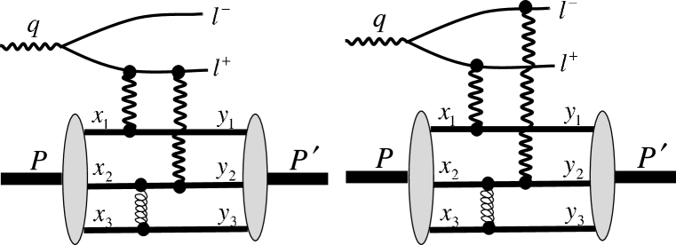
Figure 6: Typical diagrams for lepton pair production from a 3-quark proton.

$$A_{2}^{\uparrow\uparrow} \equiv A_{2}^{\gamma N\rightarrow Nl^{-}l^{+}}(\theta,\phi)$$

$$= \frac{2i\sqrt{2}\pi g^{2}e^{3}s\text{ }}{9M^{7}\rho^{5/2}(1+\rho)^{2}}e^{-i\theta}(\cos\theta+e^{-i\phi}\frac{M}{\sqrt{-t}}\sin\theta)\left[i\sqrt{\rho}(e^{i\theta}-1)+e^{i\phi}(e^{i\theta}+1)\right]^{2}\times$$

$$\;\int\left[dx\right]\left[dy\right]\frac{e_{1}(e_{2}x_{2}y_{2}+e_{3}x_{3}y_{3})\Phi(x_{1},x_{2},x_{3})\Phi(y_{1},y_{2},y_{3})x_{1}\delta(y_{1}-x_{1})}{x_{1}x_{2}x_{3}y_{1}y_{2}y_{3}\left[x_{1}\overline{x}_{1}+\Lambda\right]\overline{x}_{1}^{2}}.$$

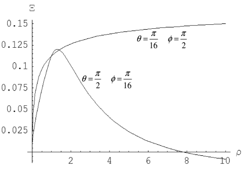
Figure 7: Lepton pair asymmetry from a proton target.

In the above (as well as in the equation below), it is implicitly understood that the complex conjugate, and exchange of labels $(1,3)\leftrightarrows(3,1)$ are to be added on. The charges $e_{i}$ are in units of the electron charge $e$ $(\alpha_{e}=e^{2}/4\pi)$. Inserting this and the single-photon results into Eq.34 yields,

$$\Theta_{N}(\theta,\phi) = -\frac{64\pi^{3}\alpha_{s}\alpha_{e}}{9(-t)^{2}G_{M}(t)}(\cos\theta+e^{-i\phi}\frac{M}{\sqrt{-t}}\sin\theta)\times$$

$$\int\left[dx\right]\left[dy\right]\frac{e_{1}(e_{2}x_{2}y_{2}+e_{3}x_{3}y_{3})\Phi(x_{1},x_{2},x_{3})\Phi(y_{1},y_{2},y_{3})x_{1}\delta(y_{1}-x_{1})}{x_{1}x_{2}x_{3}y_{1}y_{2}y_{3}\left[y_{1}\overline{y_{1}}+\Lambda\right]\overline{y_{1}}^{2}}.$$

As a check on the correctness of the calculations for scattering amplitudes for both the meson and baryon cases, we have verified that the Ward identity is satisfied in all different ways. Perturbatively $(-t)^{2}G_{M}(t)\longrightarrow$ constant at large $t$, and so again one has approximate scale invariance. In Fig. 7 we have plotted the asymmetry off a proton target. In this exploratory calculation we have used the Chernyak-Zhitnitsky wavefunction in ref.[9]. In this paper we have calculated asymmetries, not cross-sections because the latter involve a 3-body phase space. Since J-Psi photoproduction has been measured in exclusive reactions[9], lepton pair production should also be possible.

Finally we remark that Sudakov effects, which arise from the bremstrahlung of widely separated quarks that undergo large changes in momentum, will lead to a weakening of the effective coupling. Thus, although the angular structure of the amplitude will probably be similar, one must investigate diagrams that are of one order higher in $\alpha_{s}$. For the proton case this will involve a very large number of diagrams that will require a machine computation. We have not attempted this calculation.

Acknowledgments

The author thanks Stanley J. Brodsky and Xiangdong Ji for valuable comments and encouragement.

References

• [1] M.N. Rosenbluth, Phys. Rev. 79, 615 1950.
• [2] M.K.Jones et al., Phys.Rev.Lett.84, 1398 (2000); O.Gayouet al., Phys.Rev.Lett.88, 092301 (2002); V.Punjabi et al. Phys.Rev. C71:055202 (2005); Jones M.K, et al. Phys. Rev.Lett 84:1398 (2000).
• [3] P.G. Blunden, W. Melnitchouk, J.A. Tjon, Phys.Rev.C72:034612, 2005, e-Print Archive: nucl-th/0506039.
• [4] Yu-Chun Chen, Andrei V. Afanasev, Stanley J. Brodsky, Carl E. Carlson, Marc Vanderhaeghen, Phys.Rev.D72:013008, 2005 and e-Print Archive: hep-ph/0502013.
• [5] X. Ji, Phys. Rev. Lett. 78, 610 (1997); X. Ji, Phys.Rev.D55, 7114 (1997); A. V. Radyushkin, Phys.Lett.B380, 417 (1996); Phys.Lett.B385 (1996) 333; A. V. Radyushkin, Phys.Rev.D56, 5524, 1997.
• [6] C.E.H Wright and K. Jager, Ann.Rev.Nucl.Part.Sci.54:217-267,2004.
• [7] S.J.Brodsky and J.R.Gillespie, Phys. Rev. D173, 1011, 1968. This paper discusses photoproduction of lepton pairs from a nuclear target and also uses interference with the Born amplitude to generate asymmetries.
• [8] E.R. Berger, M. Diehl, B. Pire, Eur.Phys.J.C23:675-689,2002, e-Print Archive: hep-ph/0110062.
• [9] ZEUS Collaboration, Nucl.Phys. B695 (2004) 3-37, e-Print Archive: hep-ex/0404008.
• [10] R.Vega and J.Wudka, Phys.Rev.D53:5286-5292, 1996, Erratum-ibid. D56:6037-6038, 1997.
• [11] G.R.Farrar, H.Zhang, A.A.Ogloblin, and I.R.Zhitnitsky, Nucl.Phys. B311 585, 1988.
• [12] V. Braun, R.J. Fries, N. Mahnke, E. Stein, Nucl.Phys.B589:381-409,2000, Erratum-ibid.B607:433,2001.
• [13] G.P.Lepage and S.J.Brodsky, Phys.Rev.D22, 2157, 1980.
• [14] P.Hoodbhoy, X.Ji, and F.Yuan, Phys.Rev.Lett. 92: 012003, 2004, e-Print Archive: hep-ph/0309085.
• [15] A.V. Efremov and A.V.Radyushkin , Phys. Lett. 94B:245 (1980).