$Id:espcrc2.tex,v1.22004/02/2411:22:11speppingExp$ E. Gardi and J.R. Andersen

Progress in computing inclusive B decay spectra

Abstract

We review the progress in the QCD calculation of inclusive decay spectra. It was recently shown that the inherent infrared finiteness of inclusive spectra extends beyond the level of logarithms. Dressed Gluon Exponentiation makes practical use of this property by computing the Sudakov exponent as a Borel sum. Based on renormalon analysis, infrared sensitivity in the exponent is reflected in power corrections that are inversely proportional to the third power of the mass. Therefore, the parametric enhancement of non-perturbative corrections near the phase–space boundary is effective only in a small region. Consequently, the on-shell decay spectrum provides a good approximation to the meson decay. In particular, it facilitates a precise determination of $|V_{ub}|$ from present measurements of inclusive charmless semileptonic widths without involving a non-perturbative “shape function”.

One of the important challenges for QCD presented by the B factories is the calculation of inclusive partial decay widths within specific regions of phase space. The obvious example is the inclusive measurement of charmless semileptonic decay, ${\bar{B}}\longrightarrow X_{u}l\bar{\nu}$, used for the determination of $|V_{ub}|$. Owing to the overwhelming charm background, this measurement is strictly restricted to the region of small hadronic mass, $M_{X}<1.7$ GeV, where charmed final states are kinematically excluded; specific cuts within this region are adopted depending on the experimental techniques applied. Consequently, extracting $|V_{ub}|$ relies on quantitative theoretical understanding of the spectrum.

The common lore has been that estimates of the partial widths for the relevant cuts strongly depend on the non-perturbative structure of the meson. The spectrum in the small–$M_{X}$ region was obtained [1, 2, 3] through the convolution of a computable hard coefficient function with a leading–twist momentum distribution function of the b quark in the meson, the “shape function” [4, 5]. Being non-perturbative, the latter was not computed, but rather parametrized and fitted to the measured ${\bar{B}}\longrightarrow X_{s}\gamma$ spectrum, in analogy with deep inelastic (DIS) structure function phenomenology. The “shape function” has been the dominant source of uncertainty in determining $|V_{ub}|$.

Recently the situation has changed. It was shown that the inherent infrared finiteness of inclusive spectra extends beyond the level of logarithms [6]: the leading renormalon ambiguity in the Sudakov exponent cancels against that of the pole mass while the next–to–leading one is absent. Upon using Dressed Gluon Exponentiation (DGE) [7, 8, 9, 10, 11, 12] the ${\bar{B}}\longrightarrow X_{s}\gamma$ and ${\bar{B}}\longrightarrow X_{u}l\bar{\nu}$ decay spectra can be well approximated by the corresponding on-shell decay spectra [6, 15, 14, 17, 16, 13]. Non-perturbative effects associated with the meson structure enter in this framework as power corrections, and have just a small impact on the experimentally–relevant partial widths. The purpose of this talk is to explain why this is so.

Inclusive B decays such as $\bar{B}\longrightarrow X_{s}\gamma$ and $\bar{B}\longrightarrow X_{u}l\bar{\nu}$ are dominated by jet-like momentum configurations: the hadronic system $X$ has a small mass, $M_{X}\ll M_{B}$, while its energy in the B rest frame is large. Inclusive decays can be analyzed within perturbation theory owing to the fact that the heavy quark carries most of the meson momentum and it is therefore close to its mass shell. By making the perturbative, on-shell approximation one neglects non-perturbative effects that are suppressed by inverse powers of the heavy–quark mass. In the region of interest, of small $M_{X}$, these power corrections are parametrically enhanced. This will be a central issue in what follows.

Given the typical jet–like momentum configuration it is convenient to compute the spectrum in terms of lightcone coordinates. The hadronic lightcone coordinates are defined by: $P^{\pm}=E_{X}\mp|\vec{P}_{X}|$. The jet is characterized by large $P^{-}$, of ${\cal O}(M_{B})$ and small $P^{+}$, which is of the order of the mass difference between the meson and the quark, $\bar{\Lambda}=M_{B}-m_{b}$. Within the on-shell approximation, we define the partonic lightcone coordinates: $p_{j}^{\pm}=P^{\pm}-\bar{\Lambda}$. At Born level, the $p_{j}^{+}$ distribution is trivial, $\delta(p_{j}^{+})$. Beyond this order, the small $p_{j}^{+}$ region is characterized by soft and collinear gluon emission that broadens the $p_{j}^{+}$ distribution. This is why Sudakov resummation is essential in computing the spectrum.

One obvious limitation of perturbation theory is the fact that the perturbative spectrum, at any order, has support only for $p_{j}^{+}>0$, i.e. for $P^{+}>\bar{\Lambda}$, while the physical spectrum fills up the whole region down to $P^{+}=0$. As we shall see below, this inherent limitation is removed in the DGE approach [15].

In perturbation theory, the large hierarchy between $p_{j}^{+}$ and $p_{j}^{-}$ in the peak region is reflected in large Sudakov logarithms. It is convenient to choose the resummation variable as the exponent of the rapidity, $r\equiv p_{j}^{+}/p_{j}^{-}$ and write the triple differential width in $b\longrightarrow X_{u}l\bar{\nu}$ as [17]

$$\frac{1}{\Gamma_{0}}\frac{d\Gamma(\lambda,r,x_{l})}{d\lambda drdx_{l}}=V(\lambda,x_{l})\delta(r)+R(\lambda,r,x_{l}),$$ (1)

where the additional kinamatic variables are $\lambda=p_{j}^{-}/m_{b}$ and $x_{l}=2E_{l}/m_{b}$, the Born–level width is $\Gamma_{0}={G_{F}^{2}\left|V_{ub}\right|^{2}m_{b}^{5}}/{(192\pi^{3})}$, the virtual corrections are

$$V(\lambda,x_{l})=w_{0}(\lambda,x_{l})+\frac{C_{F}\alpha_{s}}{\pi}w_{1}(\lambda,x_{l})+\cdots$$ (2)

and the real–emission contribution, which starts at ${\cal O}(\alpha_{s})$, is further split as $R(\lambda,r,x_{l})=R_{\hbox{\tiny sing.}}(\lambda,r,x_{l})+R_{\hbox{\tiny reg.}}(\lambda,r,x_{l})$. The regular piece $R_{\hbox{\tiny reg.}}(\lambda,r,x_{l})$, similarly to $V(\lambda,x_{l})$, is known [20, 17] to ${\cal O}(\alpha_{s})$ only, while

$$\!R_{\hbox{\tiny sing.}}(\lambda,r,x_{l})\!=\!-w_{0}(\lambda,x_{l})\!\left(\frac{\ln r}{r}\!+\!\frac{7}{4}\frac{1}{r}\right)_{*}\!\!\!\frac{C_{F}\alpha_{s}}{\pi}\!+\!\cdots$$

which contains all the non-integrable terms at $r\longrightarrow 0$, regularized as $()_{*}$ distributions, is known in full to ${\cal O}(\alpha_{s}^{2})$ — see Eq. (3.41) in Ref. [17] — and in part, at higher orders. This higher–order information is contained in the resummation formula:

$$\frac{d\Gamma_{N}(\lambda,x_{l})}{d\lambda dx_{l}}\!\!\!\! \equiv \!\!\!\!\frac{1}{\Gamma_{0}}\int_{0}^{(1-x_{l})/\lambda}\!\!\!\!\!\!\!\!\!\!\!\!\!\!dr\left(1-r\right)^{N-1}\frac{d\Gamma(\lambda,r,x_{l})}{d\lambda drdx_{l}}$$ (3)

$$=V(\lambda,x_{l})\times{\rm Sud}(m_{b}\lambda,N)+\Delta R_{N}(\lambda,x_{l}).$$

In the small $p_{j}^{+}$ region, corresponding to large $N$, the first term dominates: it sum up to all orders perturbative corrections that diverge as powers of $\ln N$ or are finite in the $N\longrightarrow\infty$ limit. The remainder,

$$\Delta R_{N}(\lambda,x_{l})\equiv\int_{0}^{{(1-x_{l})}/{\lambda}}\!\!\!\!\!\!\!\!\!dr(1-r)^{N-1}R_{\hbox{\tiny reg.}}(r,\lambda,x_{l}),$$

is of ${\cal O}(1/N)$ and can be included at fixed order.

The resummation formula (3) is a manifestation of the infrared and collinear safety of the on-shell decay spectrum: owing to the cancellation of infrared singularities between real and virtual corrections, the moments have finite expansion coefficients to any order in perturbation theory. As usual, this cancelation leaves behind large Sudakov logarithms. These arise from two distinct subprocesses [21, 22, 6, 23]: the formation of a jet of invariant mass squared of ${\cal O}(p^{+}_{j}p^{-}_{j})$ and radiation off the nearly on-shell b–quark, characterized by transverse momenta of ${\cal O}(p^{+}_{j})$. The two corresponding functions, the jet function $J_{N}$ [24, 25, 26, 12] and the quark distribution in an on-shell heavy quark $S_{N}$ [14, 28, 27] obey the following evolution equations in moment space:

$$\frac{d\ln J_{N}(Q;\mu_{F})}{d\ln Q^{2}}=\!\!\int_{0}^{1}\!\!\frac{dr}{r}\!\!\left(\bar{r}^{N-1}-1\right){\cal J}\left(\alpha_{s}(rQ^{2})\right),$$

(4)

$$\frac{d\ln S_{N}(Q;\mu_{F})}{d\ln Q^{2}}=\!\!-\!\!\int_{0}^{1}\!\!\frac{dr}{r}\!\!\left(\bar{r}^{N-1}-1\right){\cal S}\left(\alpha_{s}(r^{2}Q^{2})\right),$$

where $\bar{r}\equiv 1-r$ and where ${\cal J}$ and ${\cal S}$ are Sudakov anomalous dimensions that are now known in full to NNLO [29, 15, 14, 28]. The Sudakov factor, summing up the logarithmically–enhanced terms in decay spectra to all orders, is: ${\rm Sud}(\lambda m_{b},N)=J_{N}(\lambda m_{b};\mu_{F})S_{N}(\lambda m_{b};\mu_{F})$, where the factorization–scale dependence cancels exactly in the product.

Note the fundamental difference with DIS structure functions where there is just one source [12] of Sudakov logarithms, namely the jet function $J_{N}(Q;\mu_{F})$, and the factorization–scale dependence cancels against the non-perturbative quark distribution function $q_{N}(\mu_{F})$, e.g. $F_{2}^{N}\sim J_{N}(Q;\mu_{F})q_{N}(\mu_{F})$. Contrary to $S_{N}$, $q_{N}$ cannot be defined in perturbation theory owing to the collinear singularity of an incoming light quark.

Because of the cancellation of logarithmic infrared singularities, the evolution kernels defined by the r.h.s. in (Progress in computing inclusive B decay spectra) are finite to any order in perturbative theory. However, these kernels conceal infrared sensitivity at the power level [30, 31, 32, 7, 8, 9, 10, 11, 12, 6, 15, 14, 17, 16, 13], which only becomes explicit once running–coupling effects are resummed to all orders [7, 8, 9, 10, 11, 12]. A systematic way to quantify this infrared sensitivity is to regularize the ensuing divergence of the perturbative expansion by Borel summation [33, 34, 35]. To this end one writes the scheme–invariant Borel representation [36] of the anomalous dimensions [7, 8, 9, 10, 11, 12, 6, 15, 14, 17, 16, 13]:

$${\cal J}\left(\alpha_{s}(\mu^{2})\right)\!=\!\frac{C_{F}}{\beta_{0}}\int_{0}^{\infty}\!du\left(\frac{\Lambda^{2}}{\mu^{2}}\right)^{u}T(u)B_{\cal J}(u),$$ (5)

$${\cal S}\left(\alpha_{s}(\mu^{2})\right)\!=\!\frac{C_{F}}{\beta_{0}}\int_{0}^{\infty}\!du\left(\frac{\Lambda^{2}}{\mu^{2}}\right)^{u}T(u)B_{\cal S}(u),$$

where $\beta_{0}=\frac{11}{12}C_{A}-\frac{1}{6}N_{f}$ and $T(u)\equiv(u\delta)^{u\delta}{\rm e}^{-u\delta}/\Gamma(1+u\delta)$ with $\delta\equiv\beta_{1}/\beta_{0}^{2}$. Using (5) in (Progress in computing inclusive B decay spectra) one can explicitly perform the $r$ integration and identify potential power–like ambiguities arising from the $r\longrightarrow 0$ limit as Borel singularities. The solution of the evolution equations, formulated as a Borel sum, is [15]:

$${\rm Sud}(\lambda m_{b},N)=\exp\bigg{\{}\frac{C_{F}}{\beta_{0}}\int_{0}^{\infty}\frac{du}{u}\,T(u)\left(\frac{\Lambda^{2}}{\lambda^{2}m_{b}^{2}}\right)^{u}$$

$$\times\bigg{[}B_{\cal S}(u)\left(\frac{\Gamma(-2u)\Gamma(N)}{\Gamma(N-2u)}+\frac{1}{2u}\right)$$ (6)

$$\hskip 30.0pt-B_{\cal J}(u)\left(\frac{\Gamma(-u)\Gamma(N)}{\Gamma(N-u)}+\frac{1}{u}\right)\bigg{]}\bigg{\}}.$$

In the jet–function part one finds potential renormalon ambiguities at positive integer values of $u$, while in the soft–function part at any integer and half integer $u$. Being anomalous dimensions, $B_{\cal J}(u)$ and $B_{\cal S}(u)$ are not expected to have any renormalon singularities of their own, however, unless these functions vanish at these locations there will be power-like ambiguities in the evolution kernels in (Progress in computing inclusive B decay spectra). These ambiguities scale as powers of $\Lambda^{2}N/(\lambda m_{b})^{2}$ and $\Lambda N/(\lambda m_{b})$, corresponding to the jet–mass and the soft scale, respectively, so they are parametrically–enhanced at large $N$.

The discussion of renormalon singularities can be made concrete by focusing on the gauge–invariant set of radiative corrections corresponding to the large–$\beta_{0}$ limit. The anomalous dimensions are then obtained as analytic functions in the Borel plane [12]:

$$\left.B_{\cal J}(u)\right|_{{\rm large}\,\beta_{0}} \!\!\!\!=\!\!\!\! \frac{{\rm e}^{\frac{5}{3}u}}{2}\left(\frac{1}{1-u}+\frac{1}{1-u/2}\right)\frac{\sin\pi u}{\pi u},$$

$$\left.B_{\cal S}(u)\right|_{{\rm large}\,\beta_{0}} \!\!\!\!=\!\!\!\! {\rm e}^{\frac{5}{3}u}(1-u).$$ (7)

Based on these expressions one can deduce which power ambiguities indeed appear in Eq. (Progress in computing inclusive B decay spectra). On the soft scale one finds ambiguities corresponding to $u=\frac{1}{2}$ and $u\geq\frac{3}{2}$ and on the jet mass scale, $u=1$ and $u=2$. Of course, these ambiguities should all cancel once non-perturbative corrections are systematically included. Conversely, in absence of a non-perturbative calculation, the ambiguities provide a good hint on the functional form, and quite possibly even the magnitude, of the non-perturbative power corrections.

Although the dominance of non-perturbative corrections that are probed by renormalons cannot be established from first principles in QCD, this conjecture has led to successful power–correction phenomenology in a variety of applications [37, 34, 39, 38]. The DGE approach was applied to several infrared and collinear safe observable, notably event–shape distributions [7, 8] and heavy–quark fragmentation [10, 11] where precise data from LEP was used to test the renormalon dominance assumption. The observed hadronization effects near the phase–space boundary were found to be in agreement with the pattern of power corrections predicted by renormalons. On these grounds one expects that the renormalon structure of the Sudakov exponent provides a good indication on non-perturbative corrections also in B decay spectra. Of course, here the leading corrections are associated with the initial–state B meson, rather than final–state hadronization, and the renormalon dominance assumption must be again confronted with data.

In computing the Sudakov factor (Progress in computing inclusive B decay spectra) we assume that the pattern of renormalon singularities of the large–$\beta_{0}$ limit holds in the full theory. Nonetheless, the perturbative expansions of these functions at $u=0$ and likewise the residues in (Progress in computing inclusive B decay spectra) get modified by ${\cal O}(1/\beta_{0})$ contributions. In order to match (Progress in computing inclusive B decay spectra) onto the perturbative expansions of ${\cal J}$ and ${\cal S}$ [14], we write the following ansatz [15, 17]:

$$B_{\cal J}(u) \!\!\!\!\!\!=\!\!\!\!\!\! \left.B_{\cal J}(u)\right|_{{\rm large}\,\beta_{0}}\times{\rm e}^{c_{1}u+c^{\cal J}_{2}u^{2}}\times W_{\cal J}(u)$$ (8)

$$B_{\cal S}(u) \!\!\!\!\!\!=\!\!\!\!\!\! \left.B_{\cal S}(u)\right|_{{\rm large}\,\beta_{0}}\times{\rm e}^{c_{1}u+c^{\cal S}_{2}u^{2}}\times W_{\cal S}(u),$$

where $c_{1}=\left(1-{\pi^{2}}/{4}\right){C_{A}}/({3\beta_{0}})$ is universal [27], $c^{{\cal J}/{\cal S}}_{2}$ are determined based on the known NNLO expansions of these functions and $W_{{{\cal J}/{\cal S}}}(u)$ parametrize yet–unknown ${\cal O}(u^{3})$ corrections. By fixing $B_{\cal S}(u)$ and $B_{\cal J}(u)$ this way and choosing the Principal Value prescription for the renormalons, the Sudakov factor (Progress in computing inclusive B decay spectra) is uniquely determined.

Now, the resummed spectrum is obtained by an inverse Mellin transformation of Eq. (3),

$$\frac{1}{\Gamma_{0}}\frac{d\Gamma(\lambda,r,x_{l})}{d\lambda drdx_{l}}=\int_{\cal C}\frac{dN}{2\pi i}\left(1-{r}\right)^{-N}\!\frac{d\Gamma_{N}(\lambda,x_{l})}{d\lambda dx_{l}},$$ (9)

where the integration contour ${\cal C}$ runs parallel to the imaginary axis, to the right of the singularities of the integrand. Finally, the triple differential distribution in physical, hadronic variables is:

$$\frac{1}{\Gamma_{0}}\frac{d\Gamma(P^{+},\,P^{-},\,E_{l})}{dP^{+}\,dP^{-}\,dE_{l}}=\frac{2}{\lambda m_{b}^{3}}\,\times$$ (10)

$$\left.\frac{1}{\Gamma_{0}}\frac{d\Gamma(\lambda,r,x_{l})}{d\lambda drdx_{l}}\right|_{\left\{r=\frac{P^{+}-\bar{\Lambda}}{P^{-}-\bar{\Lambda}};\,\lambda=\frac{P^{-}-\bar{\Lambda}}{m_{b}};\,x_{l}=\frac{2E_{l}}{m_{b}}\right\}}.$$

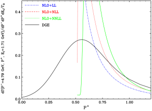
Figure 1: The $P^{+}$ spectrum in $\bar{B}\longrightarrow X_{u}l\bar{\nu}$ in the on-shell approximation at a representative point in phase space: $P^{-}=4.79$ GeV; $E_{l}=1.71$ GeV. The spectrum is computed with fixed logarithmic accuracy (LL, NLL, NNLL) and by DGE. All results are matched to NLO [17].

The change of variables in (10) has a subtle but absolutely crucial role in obtaining the correct distribution within the on-shell approximation. To understand it observe that this transformation involves $\bar{\Lambda}\equiv M_{B}-m_{b}$ that is ambiguous since the pole mass $m_{b}$ has a $u=\frac{1}{2}$ renormalon [18, 19], and recall that the Sudakov exponent in (Progress in computing inclusive B decay spectra) also has a $u=\frac{1}{2}$ renormalon ambiguity. These ambiguities have the same source namely the ambiguous definition of an on-shell state and they cancel out exactly [6] in Eq. (10). This cancellation was checked explicitly in the large–$\beta_{0}$ limit and it is understood to be general. In the course of the calculation we deal with it by using the Principal Value Borel sum regularization in both Eq. (Progress in computing inclusive B decay spectra) and in the calculation of the pole mass [15] in $\bar{\Lambda}$.

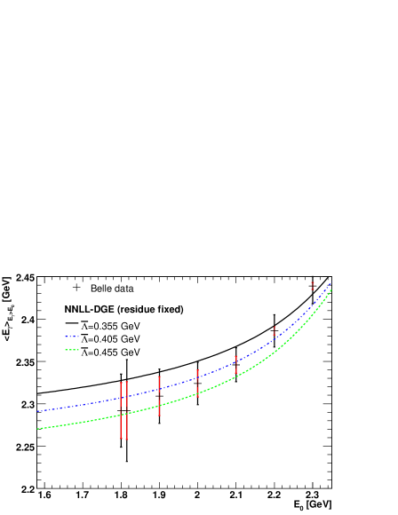
Figure 2: The average energy in $\bar{B}\longrightarrow X_{s}\gamma$, $\left<E_{\gamma}\right>$, in the on-shell approximation, as a function of the minimum photon energy cut $E_{0}$, as calculated by DGE in [15] varying $m_{b}^{\hbox{\tiny${\overline{\rm MS}}$}}$ within its error range. The result is compared with data from Belle [42]. Inner and total error bars show systematic and statistical plus systematic errors (added in quadrature), respectively.

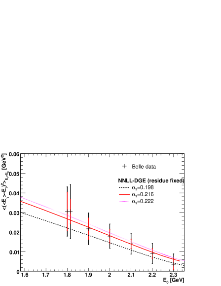
Figure 3: The energy variance in $\bar{B}\longrightarrow X_{s}\gamma$, $\left<(\left<E_{\gamma}\right>-E_{\gamma})^{2}\right>$, as a function of the minimum photon energy cut $E_{0}$, as calculated by DGE in [15] varying $\alpha_{s}$ within its error range, compared with data from Belle [42].

The extent to which the perturbative on-shell spectrum is constrained depends primarily on having the soft anomalous dimension function $B_{\cal S}(u)$ entering Eq. (Progress in computing inclusive B decay spectra) sufficiently well under control. Eq. (8) incorporates the QCD perturbative expansion of $B_{\cal S}(u)$ around the origin up to NNLO. However, owing to the soft scales probed as $N$ gets large, which are ${\cal O}(\lambda m_{b}/N)$, the Borel sum has some sensitivity to $B_{\cal S}(u)$ away from the origin. This sensitivity depends on what is assumed about $W_{\cal S}(u)$ in Eq. (8). Here one can make use [15] of additional information, namely the value of the leading renormalon residue of the pole mass, which fixes $B_{\cal S}(u=\frac{1}{2})$ owing to the exact cancellation of ambiguities explained above. We further assume that $W_{\cal S}(u)$ has no Borel singularities and thus the vanishing of $\left.B_{\cal S}\right|_{{\rm large}\,\beta_{0}}(u=1)$ carries over to the full theory. It was shown [15, 17] that so long as $B_{\cal S}(u)$ does not get particularly large beyond this region, e.g. near the $u=\frac{3}{2}$ renormalon position, the Principal Values Borel sum in Eq. (Progress in computing inclusive B decay spectra) is well under control. Moreover, the resulting spectrum in hadronic variables (10) has approximately the correct physical support properties, i.e. it smoothly extends into the non-perturbative region $P^{+}<\bar{\Lambda}$ and vanishes for $P^{+}\mathrel{\mathchoice{\vbox{\offinterlineskip\halign{$\m@th\displaystyle\hfil#\hfil$\cr<\crcr\sim\crcr} }}{\vbox{\offinterlineskip\halign{$\m@th\textstyle\hfil#\hfil$\cr<\crcr\sim\crcr} }}{\vbox{\offinterlineskip\halign{$\m@th\scriptstyle\hfil#\hfil$\cr<\crcr\sim\crcr} }}{\vbox{\offinterlineskip\halign{$\m@th\scriptscriptstyle\hfil#\hfil$\cr<\crcr\sim\crcr} }}}0$. This highly non-trivial property of the Borel–resummed on-shell spectrum suggests that non-perturbative corrections in this framework are not large.

Having obtained this result through resummation, it is interesting to return to the conventional Sudakov resummation framework, in which Eq. (Progress in computing inclusive B decay spectra) is expanded and computed to a given logarithmic accuracy, and see why it fails. The comparison between the results is shown in Fig. 1. Obviously, there is a qualitative difference: the fixed–logarithmic–accuracy curves are sharply peaked reaching a Landau singularity near $P^{+}=0.5$ GeV where they become complex; in contrast, the DGE result, which is not affected by Landau singularities, smoothly extends to the non-perturbative regime $P^{+}<\bar{\Lambda}\simeq 0.4$ GeV. Aside from the Landau singularity issue, one observes that results of increasing logarithmic accuracy represent a badly divergent series, which is dominated by the leading $u=\frac{1}{2}$ renormalon. The divergence sets in early (see Tables 1 and 2 in Ref. [16]) and therefore increasing the formal accuracy in this naive approach may result in worse approximations. In contrast, in the DGE approach the renormalon is regularized and the associated ambiguity cancels.

Eventually, the dependence of the on-shell decay spectrum on the adopted Principal Value prescription concerns renormalons at $u=k/2$, with all integer $k\geq 3$. These give rise to ambiguities scaling as powers of $\left(\Lambda N/(\lambda m_{b})\right)^{k}$. The corresponding power corrections can be summed up into a non-perturbative “shape function”, ${\cal F}\left(\Lambda N/(\lambda m_{b})\right)$, which multiplies the Sudakov factor. This function has a clear field–theoretic interpretation as the moment space ratio between the quark distribution in the meson and that in an on-shell heavy quark [6]. A priori, power corrections on the soft scale could affect the entire peak region. However, based on the renormalon ambiguities we actually find the situation is quite different: the absence of the first two powers and the inherent suppression of higher powers that is dictated by the structure of Sudakov exponent (Eqs. (3.50) and (3.51) in Ref. [17]) suggest that the shape function should mainly affect high moments $N>\lambda m_{b}/\Lambda$ and therefore be important only in the close vicinity of the endpoint, $P^{+}\longrightarrow 0$. It amounts to small corrections elsewhere.

Given the properties of the resummed spectrum and the relatively minor role of non-perturbative corrections in this approach, one can directly use the perturbative on-shell result as an approximation to the meson decay spectrum; in this approximation ${\cal F}\left(\Lambda N/(\lambda m_{b})\right)=1$. This was suggested in Ref. [15] where predictions for the $\bar{B}\longrightarrow X_{s}\gamma$ spectrum were obtained. In addition the first few central moments with a varying lower cut on the photon energy were computed. Soon after, first results for these moments were published by the BaBar collaboration, which agree well with the predictions — see Fig. 4 in [16]. A similar comparison with Belle results [42] was done later on and is shown in Figs. 2 and 3.

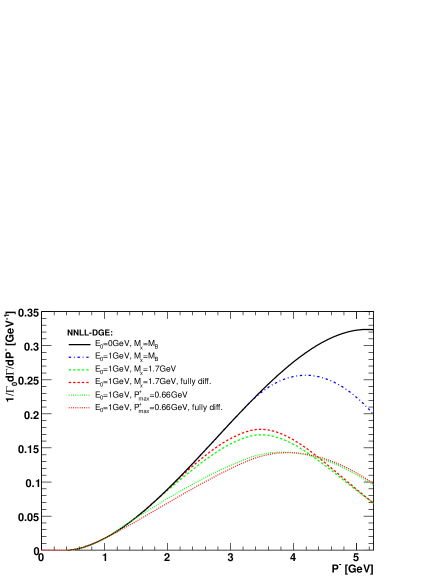
Figure 4: The $P^{-}$ spectrum in $\bar{B}\longrightarrow X_{u}l\bar{\nu}$ as calculated by DGE [17], after integration over $P^{+}$ and $E_{l}$ in four different situations: no cuts (full), $E_{l}>1$ GeV cut only (dotdashes), $E_{l}>1$ GeV with $P^{+}P^{-}<M_{X}^{2}=(1.7\,{\rm GeV})^{2}$ (dashes), and $E_{l}>1$ GeV with $P^{+}<P^{+}_{\max}=0.66$ GeV (dots).

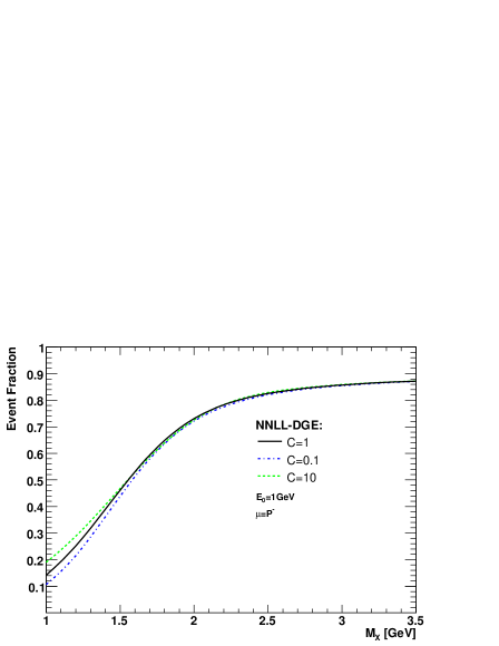
Figure 5: The event fraction in $\bar{B}\longrightarrow X_{u}l\bar{\nu}$ within the range $P^{+}P^{-}<M_{X}^{2}$ and $E_{l}>1$ GeV, as calculated by DGE, plotted as a function of the cut value $M_{X}$. Different assignments for the unknown parameter $C$ (see Sec. 3.2 in [17]), which is proportional to $B_{\cal S}(u=\frac{3}{2})$, are used.

The good agreement [16] of the on-shell calculation with the measured $\bar{B}\longrightarrow X_{s}\gamma$ decay spectrum provided a strong incentive to apply this approach to $\bar{B}\longrightarrow X_{u}l\bar{\nu}$. This was done in Ref. [17] where $|V_{ub}|$ was extracted for the first time directly based on resummed perturbation theory, without relying on any parametrization of the spectral shape. As explained above, the resummation applies to the fully differential width. This means that the measurement of any partial branching fraction can be readily translated into a measurement of $|V_{ub}|$.

Fig. 4 presents the computed event–fraction as a function of $P^{-}$. It shows the distribution for two cuts that have been used by Belle [43] to discriminate charm: an upper cut on the hadronic invariant mass at $M_{X}=1.7$ GeV, and an upper cut on $P^{+}$, at $P^{+}_{\max}=0.66$ GeV. In both cases a lower cut on the lepton energy $E_{l}>1\,{\rm GeV}$ is applied as well. Belle data in these measurements are:

$$\Delta{\cal B}(P^{+}P^{-}<(1.7\,{\rm GeV})^{2})={1.24\cdot 10^{-3}}\,\,(\pm 13.4\%)$$

$$\Delta{\cal B}(P^{+}<0.66\,{\rm GeV})={1.10\cdot 10^{-3}}\,\,(\pm 17.2\%),$$

where the numbers in the brackets represent the total experimental error. The DGE results for the corresponding event fractions are:

$${R_{\rm cut}}(P^{+}P^{-}<(1.7\,{\rm GeV})^{2})={0.615}\,\,(\pm 9.6\%)$$

$${R_{\rm cut}}(P^{+}<0.66\,{\rm GeV})={0.535}\,\,(\pm 15.2\%).$$

Using

$$\Delta{\cal B}({\bar{B}\longrightarrow X_{u}l\bar{\nu}}\,\,{\rm{restricted}\,\,phase\,\,space})$$

$$=\tau_{B}{\Gamma_{\hbox{\tiny tot}}}\left({\bar{B}\longrightarrow X_{u}l\bar{\nu}}\right)\times{R_{\rm cut}},$$ (11)

and $\Gamma_{\hbox{\tiny tot}}\left(\bar{B}\longrightarrow X_{u}l\bar{\nu}\right)={\left|V_{ub}\right|^{2}}\times 66.5\pm 4\,{\rm ps}^{-1}$, we obtain [17]

$$\left|V_{ub}\right| = \Big{(}4.35\,\pm\,0.28_{[{\rm exp}]}\,\pm\,0.26_{[{\rm th}]}\Big{)}\cdot 10^{-3}$$

$$\left|V_{ub}\right| = \Big{(}4.39\,\pm\,0.36_{[{\rm exp}]}\,\pm\,0.40_{[{\rm th}]}\Big{)}\cdot 10^{-3},$$

respectively. The largest source of uncertainty, in both the calculation of the total width and in that of the event fraction, is the value of the short–distance mass $m_{b}^{\hbox{\tiny${\overline{\rm MS}}$}}$. Apart from a precise mass, to further improve this determination it would be necessary to have a complete NNLO perturbative calculation to the fully differential width. Importantly, we find that the sensitivity to the details of the quark distribution function is small. An estimate of this source of uncertainty was obtained in Ref. [17] by changing $W_{\cal S}(u)$ in Eq. (8). Fig. 5 shows the result as a function of the $M_{X}$ cut. Evidently, the effect is small for experimentally relevant cuts.

Needless to say, the potential of the DGE approach is far from being exhausted by this perturvative determination of $\left|V_{ub}\right|$. In order to quantify the leading power corrections that constitute ${\cal F}\left(\Lambda N/(\lambda m_{b})\right)$ one would obviously need careful comparison with the measured spectrum. Both $\bar{B}\longrightarrow X_{s}\gamma$ and $\bar{B}\longrightarrow X_{u}l\bar{\nu}$ decays can be used for this purpose.

To conclude, we have shown that by properly resumming the perturbative expansion, the on-shell approximation provides reliable predictions for inclusive B decay spectra, facilitating a precise determination of $\left|V_{ub}\right|$. The calculation of the Sudakov exponent as a Borel sum guarantees renormalization and factorization scale invariance, and opens the way for incorporating valuable information on the large–order behavior of the series. At the end of the day, the main advantage of this approach stems from the possibility to use the inherent infrared safety of decay spectra, which extends beyond logarithmic accuracy.

References

- [1] A. F. Falk, Z. Ligeti and M. B. Wise, Phys. Lett. B406 (1997) 225 [hep-ph/9705235].
- [2] I. I. Y. Bigi, R. D. Dikeman and N. Uraltsev, Eur. Phys. J. C4 (1998) 453 [hep-ph/9706520].
- [3] B. O. Lange, M. Neubert and G. Paz, Phys. Rev. D72, 073006 (2005) [hep-ph/0504071].
- [4] M. Neubert, Phys. Rev. D49 (1994) 4623; [hep-ph/9312311]. Phys. Rev. D49 (1994) 3392 [hep-ph/9311325].
- [5] I. I. Y. Bigi, M. A. Shifman, N. G. Uraltsev and A. I. Vainshtein, Int. J. Mod. Phys. A9 (1994) 2467 [hep-ph/9312359].
- [6] E. Gardi, JHEP 0404, 049 (2004) [hep-ph/0403249].
- [7] E. Gardi and J. Rathsman, Nucl. Phys. B609 (2001) 123 [hep-ph/0103217];
- [8] E. Gardi and J. Rathsman, Nucl. Phys. B638 (2002) 243 [hep-ph/0201019].
- [9] E. Gardi, Nucl. Phys. B622 (2002) 365 [hep-ph/0108222].
- [10] M. Cacciari and E. Gardi, Nucl. Phys. B664 (2003) 299 [hep-ph/0301047].
- [11] E. Gardi and M. Cacciari, Eur. Phys. J. C33 (2004) S876 [hep-ph/0308235].
- [12] E. Gardi and R. G. Roberts, Nucl. Phys. B653, 227 (2003) [hep-ph/0210429].
- [13] E. Gardi, “Inclusive B decay spectra and IR renormalons”, Proceedings of ‘Workshop on Continuous Advances in QCD 2004’, Minneapolis, Minnesota, 13-16 May 2004. published by World Scientific, T. Gherghetta (Ed.) [hep-ph/0407322].
- [14] E. Gardi, JHEP 0502 (2005) 053 [hep-ph/0501257].
- [15] J. R. Andersen and E. Gardi, JHEP 0506 (2005) 030 [hep-ph/0502159].
- [16] E. Gardi and J. R. Andersen, “A new approach to inclusive decay spectra,” presented at 40th Rencontres de Moriond on QCD and High Energy Hadronic Interactions, La Thuile, Aosta Valley, Italy, 12-19 Mar 2005 [hep-ph/0504140].
- [17] J. R. Andersen and E. Gardi, JHEP 0601 (2006) 097 [hep-ph/0509360].
- [18] M. Beneke and V. M. Braun, Nucl. Phys. B426, 301 (1994) [hep-ph/9402364].
- [19] I. I. Y. Bigi, M. A. Shifman, N. G. Uraltsev and A. I. Vainshtein, Phys. Rev. D50, 2234 (1994) [hep-ph/9402360].
- [20] F. De Fazio and M. Neubert, JHEP 9906 (1999) 017 [hep-ph/9905351].
- [21] G. P. Korchemsky and G. Sterman, Phys. Lett. B340 (1994) 96 [hep-ph/9407344].
- [22] C. W. Bauer, S. Fleming, D. Pirjol and I. W. Stewart, Phys. Rev. D63 (2001) 114020 [hep-ph/0011336].
- [23] S. W. Bosch, B. O. Lange, M. Neubert and G. Paz, Nucl. Phys. B699 (2004) 335 [hep-ph/0402094].
- [24] G. Sterman, Nucl. Phys. B281 (1987) 310.
- [25] S. Catani and L. Trentadue, Nucl. Phys. B327 (1989) 323.
- [26] H. Contopanagos, E. Laenen and G. Sterman, Nucl. Phys. B484, 303 (1997) [hep-ph/9604313].
- [27] G. P. Korchemsky and A. V. Radyushkin, Nucl. Phys. B283 (1987) 342; Phys. Lett. B279 (1992) 359 [hep-ph/9203222].
- [28] G. P. Korchemsky and G. Marchesini, Nucl. Phys. B406 (1993) 225 [hep-ph/9210281].
- [29] S. Moch, J. A. M. Vermaseren and A. Vogt, Nucl. Phys. B688 (2004) 101 [hep-ph/0403192].
- [30] H. Contopanagos and G. Sterman, Nucl. Phys. B419 (1994) 77 [hep-ph/9310313].
- [31] A. G. Grozin and G. P. Korchemsky, Phys. Rev. D53 (1996) 1378 [hep-ph/9411323].
- [32] G. P. Korchemsky and G. Sterman, Nucl. Phys. B437 (1995) 415 [hep-ph/9411211].
- [33] A. H. Mueller, Nucl. Phys. B250 (1985) 327.
- [34] M. Beneke, Phys. Rept. 317, 1 (1999) [hep-ph/9807443].
- [35] M. Beneke and V. M. Braun, Nucl. Phys. B454, 253 (1995) [hep-ph/9506452].
- [36] G. Grunberg, Phys. Lett. B304 (1993) 183.
- [37] Y. L. Dokshitzer, G. Marchesini and B. R. Webber, Nucl. Phys. B469 (1996) 93 [hep-ph/9512336].
- [38] E. Gardi and G. Grunberg, JHEP 9911 (1999) 016 [hep-ph/9908458].
- [39] M. Dasgupta and G. P. Salam, J. Phys. G30 (2004) R143 [hep-ph/0312283].
- [40] A. Pineda, JHEP 0106 (2001) 022 [hep-ph/0105008].
- [41] T. Lee, Phys. Lett. B563, 93 (2003) [hep-ph/0212034].
- [42] K. Abe et al. [Belle Collaboration], “Moments of the photon energy spectrum from B X/s gamma decays measured by Belle,” [hep-ex/0508005].
- [43] I. Bizjak et al. [BELLE Collaboration], “Measurement of the inclusive charmless semileptonic partial branching fraction of B mesons and determination of V(ub) using the full reconstruction tag,” [hep-ex/0505088].