Abstract

In this article, we calculate the axial and the induced pseudoscalar form-factors $G_{A}(t=-Q^{2})$ and $G_{P}(t=-Q^{2})$ of the nucleons in the framework of the light-cone QCD sum-rules approach up to twist-6 three valence quark light-cone distribution amplitudes, and observe that the form-factors $G_{A}(t=-Q^{2})$ and $G_{P}(t=-Q^{2})$ at intermediate and large momentum transfers with $Q^{2}>2GeV^{2}$ have significant contributions from the end-point (soft) terms. The numerical values for the axial form-factor $G_{A}(t=-Q^{2})$ are compatible with the experimental data and theoretical calculations, for example, the chiral quark models and lattice QCD. The numerical values for the induced pseudoscalar form-factor $G_{P}(t=-Q^{2})$ are compatible with the calculation from the Bethe-Salpeter equation.

PACS : 12.38.Aw, 12.38.-t, 14.20.Dh

Key Words: Axial-vector current, Light-cone QCD sum rules, Form-factor

1 Introduction

The axial and induced pseudoscalar form-factors of the nucleons are of fundamental importance in studying the weak interactions and the pion-nucleon scattering. They provide an important test for theories which attempt to describe the under-structures of the nucleons and the underlying dynamics [1, 2]. Using Lorentz covariance and chiral symmetry, the matrix element of the axial-vector current between the initial and final nucleon states excluding the second class current [3] can be parameterized as,

$$\langle N(P^{\prime})|A_{\mu}^{a}(0)|N(P)\rangle=N(P^{\prime})\left\{\gamma_{\mu}G_{A}(t)+\frac{(P^{\prime}-P)_{\mu}}{2M}G_{P}(t)\right\}\gamma_{5}\tau^{a}N(P),$$ (1)

here the $\tau^{a}$ is the Pauli matrix, the $M$ is the average mass for the proton and neutron, $t=(P^{\prime}-P)^{2}$, the $G_{A}(t)$ and $G_{P}(t)$ are the axial and induced pseudoscalar form-factor respectively. The Goldberger-Treiman relation [4] relates the form factors $G_{A}(t)$ and $G_{P}(t)$, and the pion decay constant $f_{\pi}$,

$$g_{\pi NN}={g_{A}M\over f_{\pi}},\ \ \ g_{\pi NN}=G_{P}(t=m_{\pi}^{2}),\ \ \ g_{A}=G_{A}(t=0)\,.$$ (2)

In this article, we calculate the axial form-factor $G_{A}(t)$ and induced pseudoscalar form-factor $G_{P}(t)$ of the nucleons in the framework of the light-cone sum rules (LCSR) approach [5, 6] which combine the standard techniques of the QCD sum rules with the conventional parton distribution amplitudes describing the hard exclusive processes[7]. In the LCSR approach, the short-distance operator product expansion with the vacuum condensates of increasing dimensions is replaced by the light-cone expansion with the distribution amplitudes (which correspond to the sum of an infinite series of operators with the same twist) of increasing twists to parameterize the non-perturbative QCD vacuum, while the contributions from the hard re-scattering can be correctly incorporated as the $O(\alpha_{s})$ corrections [8]. In recent years, there have been a lot of applications of the LCSR to the mesons, for example, the form-factors, strong coupling constants and hadronic matrix elements [6], the applications to the baryons are cumbersome and only the electromagnetic form factors [9], the scalar form-factor [10] and the weak decay $\Lambda_{b}\to p\ell\nu_{\ell}$ [11] are studied, the higher twists distribution amplitudes of the baryons were not available until recently [13].

The article is arranged as follows: we derive the light-cone sum rules for the axial and induced pseudoscalar form-factors $G_{A}(t)$ and $G_{P}(t)$ of the nucleons in section II; in section III, numerical results and discussion; section VI is reserved for conclusion.

2 Light-cone sum rules for the form-factors $G_{A}(t)$ and $G_{P}(t)$

In the following, we write down the two-point correlation function $\Pi_{\mu}(P,q)$ in the framework of the LCSR approach,

$$\Pi_{\mu}(P,q) = i\int d^{4}x\,e^{iq\cdot x}\langle 0|T\left\{\eta(0)J_{\mu}(x)\right\}|P\rangle,$$ (3)

with the axial-vector current

$$J_{\mu}(x) = \bar{d}(x)\gamma_{\mu}\gamma_{5}u(x),$$ (4)

and the neutron current [12]

$$\eta(0) = \epsilon^{ijk}\left[d^{i}(0)C\!\not\!{z}d^{j}(0)\right]\,\gamma_{5}\!\not\!{z}u^{k}(0)\,,$$

$$\langle 0|\eta(0)|P\rangle = f_{\rm N}\,(P\cdot z)\!\not\!{z}N(P)\,,$$ (5)

here the $z$ is a light-cone vector, $z^{2}=0$, and the $f_{N}$ is the coupling constant of the leading twist light-cone distribution amplitude [14]. At the large Euclidean momenta ${P^{\prime}}^{2}=(P-q)^{2}$ and $q^{2}=-Q^{2}$, the correlation function $\Pi_{\mu}(P,q)$ can be calculated in perturbation theory. In calculation, we need the following light-cone expanded quark propagator [15],

$$S(x) = \frac{i\Gamma(d/2)\not\!x}{2\pi^{2}(-x^{2})^{d/2}}$$ (6)

$$+ \frac{i\Gamma(d/2-1)}{16\pi^{2}(-x^{2})^{d/2-1}}\int\limits_{0}^{1}dv\Big{\{}(1-v)\not\!x\sigma_{\mu\nu}G^{\mu\nu}(vx)+v\sigma_{\mu\nu}G^{\mu\nu}(vx)\!\not\!x\Big{\}}+...,$$

where $G_{\mu\nu}=g_{s}G_{\mu\nu}^{a}(\lambda^{a}/2)$ is the gluon field strength tensor and $d$ is the space-time dimension. The contributions proportional to the $G_{\mu\nu}$ can give rise to four-particle (and five-particle) nucleon distribution amplitudes with a gluon (or quark-antiquark pair) in addition to the three valence quarks, their corrections are usually not expected to play any significant roles [16] and neglected here [9, 11]. In the parton model, at large momentum transfers, the electromagnetic and weak currents interact with the almost free partons in the nucleons. Employ the ”free” light-cone quark propagator in the correlation function $\Pi_{\mu}(P,q)$, we obtain

$$z^{\mu}\Pi_{\mu}(P,q) = -2\int d^{4}x\,\frac{z\cdot xe^{iq\cdot x}}{\pi^{2}x^{4}}(\gamma_{5}\!\not\!{z})^{\lambda\alpha}(C\!\not\!{z}\gamma_{5})^{\beta\gamma}\epsilon^{ijk}\langle 0|T\left\{u^{i}_{\alpha}(0)u^{j}_{\beta}(x)d^{k}_{\gamma}(0)\right\}|P\rangle.$$

In the light-cone limit $x^{2}\to 0$, the remaining three-quark operator sandwiched between the proton state and the vacuum can be written in terms of the nucleon distribution amplitudes [12, 13, 14]. The three valence quark components of the nucleon distribution amplitudes are defined by the matrix element,

$$4\langle 0|\epsilon^{ijk}u_{\alpha}^{i}(a_{1}x)u_{\beta}^{j}(a_{2}x)u_{\gamma}^{k}(a_{3}x)|P\rangle=\mathcal{S}_{1}MC_{\alpha\beta}(\gamma_{5}N)_{\gamma}+\mathcal{S}_{2}M^{2}C_{\alpha\beta}(\hbox to0.0pt{/\hss}x\gamma_{5}N)_{\gamma}$$

$${}+\mathcal{P}_{1}M(\gamma_{5}C)_{\alpha\beta}N_{\gamma}+\mathcal{P}_{2}M^{2}(\gamma_{5}C)_{\alpha\beta}(\hbox to0.0pt{/\hss}xN)_{\gamma}+(\mathcal{V}_{1}+\frac{x^{2}M^{2}}{4}\mathcal{V}_{1}^{M})(\hbox to0.0pt{/\hss}PC)_{\alpha\beta}(\gamma_{5}N)_{\gamma}$$

$${}+\mathcal{V}_{2}M(\hbox to0.0pt{/\hss}PC)_{\alpha\beta}(\hbox to0.0pt{/\hss}x\gamma_{5}N)_{\gamma}+\mathcal{V}_{3}M(\gamma_{\mu}C)_{\alpha\beta}(\gamma^{\mu}\gamma_{5}N)_{\gamma}+\mathcal{V}_{4}M^{2}(\hbox to0.0pt{/\hss}xC)_{\alpha\beta}(\gamma_{5}N)_{\gamma}$$

$${}+\mathcal{V}_{5}M^{2}(\gamma_{\mu}C)_{\alpha\beta}(i\sigma^{\mu\nu}x_{\nu}\gamma_{5}N)_{\gamma}+\mathcal{V}_{6}M^{3}(\hbox to0.0pt{/\hss}xC)_{\alpha\beta}(\hbox to0.0pt{/\hss}x\gamma_{5}N)_{\gamma}$$

$${}+(\mathcal{A}_{1}+\frac{x^{2}M^{2}}{4}\mathcal{A}_{1}^{M})(\hbox to0.0pt{/\hss}P\gamma_{5}C)_{\alpha\beta}N_{\gamma}+\mathcal{A}_{2}M(\hbox to0.0pt{/\hss}P\gamma_{5}C)_{\alpha\beta}(\hbox to0.0pt{/\hss}xN)_{\gamma}+\mathcal{A}_{3}M(\gamma_{\mu}\gamma_{5}C)_{\alpha\beta}(\gamma^{\mu}N)_{\gamma}$$

$${}+\mathcal{A}_{4}M^{2}(\hbox to0.0pt{/\hss}x\gamma_{5}C)_{\alpha\beta}N_{\gamma}+\mathcal{A}_{5}M^{2}(\gamma_{\mu}\gamma_{5}C)_{\alpha\beta}(i\sigma^{\mu\nu}x_{\nu}N)_{\gamma}+\mathcal{A}_{6}M^{3}(\hbox to0.0pt{/\hss}x\gamma_{5}C)_{\alpha\beta}(\hbox to0.0pt{/\hss}xN)_{\gamma}$$

$${}+(\mathcal{T}_{1}+\frac{x^{2}M^{2}}{4}\mathcal{T}_{1}^{M})(P^{\nu}i\sigma_{\mu\nu}C)_{\alpha\beta}(\gamma^{\mu}\gamma_{5}N)_{\gamma}+\mathcal{T}_{2}M(x^{\mu}P^{\nu}i\sigma_{\mu\nu}C)_{\alpha\beta}(\gamma_{5}N)_{\gamma}$$

$${}+\mathcal{T}_{3}M(\sigma_{\mu\nu}C)_{\alpha\beta}(\sigma^{\mu\nu}\gamma_{5}N)_{\gamma}+\mathcal{T}_{4}M(P^{\nu}\sigma_{\mu\nu}C)_{\alpha\beta}(\sigma^{\mu\rho}x_{\rho}\gamma_{5}N)_{\gamma}$$

$${}+\mathcal{T}_{5}M^{2}(x^{\nu}i\sigma_{\mu\nu}C)_{\alpha\beta}(\gamma^{\mu}\gamma_{5}N)_{\gamma}+\mathcal{T}_{6}M^{2}(x^{\mu}P^{\nu}i\sigma_{\mu\nu}C)_{\alpha\beta}(\hbox to0.0pt{/\hss}x\gamma_{5}N)_{\gamma}$$

$${}+\mathcal{T}_{7}M^{2}(\sigma_{\mu\nu}C)_{\alpha\beta}(\sigma^{\mu\nu}\hbox to0.0pt{/\hss}x\gamma_{5}N)_{\gamma}+\mathcal{T}_{8}M^{3}(x^{\nu}\sigma_{\mu\nu}C)_{\alpha\beta}(\sigma^{\mu\rho}x_{\rho}\gamma_{5}N)_{\gamma}\,\,.$$ (8)

The calligraphic distribution amplitudes do not have definite twist and can be related to the ones with definite twist as

$$\mathcal{S}_{1}=S_{1},\hskip 22.76228pt2P\cdot x\mathcal{S}_{2}=S_{1}-S_{2},$$

$$\mathcal{P}_{1}=P_{1},\hskip 22.76228pt2P\cdot x\mathcal{P}_{2}=P_{1}-P_{2}$$

for the scalar and pseudoscalar distribution amplitudes,

$$\mathcal{V}_{1}=V_{1},\hskip 68.28644pt2P\cdot x\mathcal{V}_{2}=V_{1}-V_{2}-V_{3},$$

$$2\mathcal{V}_{3}=V_{3},\hskip 62.59596pt4P\cdot x\mathcal{V}_{4}=-2V_{1}+V_{3}+V_{4}+2V_{5},$$

$$4P\cdot x\mathcal{V}_{5}=V_{4}-V_{3},\hskip 14.22636pt(2P\cdot x)^{2}\mathcal{V}_{6}=-V_{1}+V_{2}+V_{3}+V_{4}+V_{5}-V_{6}$$

for the vector distribution amplitudes,

$$\mathcal{A}_{1}=A_{1},\hskip 68.28644pt2P\cdot x\mathcal{A}_{2}=-A_{1}+A_{2}-A_{3},$$

$$2\mathcal{A}_{3}=A_{3},\hskip 62.59596pt4P\cdot x\mathcal{A}_{4}=-2A_{1}-A_{3}-A_{4}+2A_{5},$$

$$4P\cdot x\mathcal{A}_{5}=A_{3}-A_{4},\hskip 14.22636pt(2P\cdot x)^{2}\mathcal{A}_{6}=A_{1}-A_{2}+A_{3}+A_{4}-A_{5}+A_{6}$$

for the axial vector distribution amplitudes, and

$$\mathcal{T}_{1}=T_{1},\hskip 109.54327pt2P\cdot x\mathcal{T}_{2}=T_{1}+T_{2}-2T_{3},$$

$$2\mathcal{T}_{3}=T_{7},\hskip 104.70593pt2P\cdot x\mathcal{T}_{4}=T_{1}-T_{2}-2T_{7},$$

$$2P\cdot x\mathcal{T}_{5}=-T_{1}+T_{5}+2T_{8},\hskip 14.22636pt(2P\cdot x)^{2}\mathcal{T}_{6}=2T_{2}-2T_{3}-2T_{4}+2T_{5}+2T_{7}+2T_{8},$$

$$4P\cdot x\mathcal{T}_{7}=T_{7}-T_{8},\hskip 54.06006pt(2P\cdot x)^{2}\mathcal{T}_{8}=-T_{1}+T_{2}+T_{5}-T_{6}+2T_{7}+2T_{8}$$

for the tensor distribution amplitudes. The light-cone distribution amplitudes $F=V_{i}$, $A_{i}$, $T_{i}$, $S_{i}$, $P_{i}$ can be represented as

$$F(a_{i}p\cdot x)=\int\mathcal{D}xe^{-ip\cdot x\Sigma_{i}x_{i}a_{i}}F(x_{i})\;,$$ (9)

with

$$\mathcal{D}x=dx_{1}dx_{2}dx_{3}\delta(x_{1}+x_{2}+x_{3}-1).$$

The distribution amplitudes are scale dependent and can be expanded with the operators of increasing conformal spin, we write down the explicit expressions for the $V_{i}$, $A_{i}$, $T_{i}$, $S_{i}$ and $P_{i}$ up to the next-to-leading conformal spin accuracy in the appendix [13, 11]; in the following, we will denote ”the light-cone distribution amplitudes including the next-to-leading conformal spin” as ”the $P$-wave approximation”. The $V_{1}$, $A_{1}$ and $T_{1}$ are the leading twist-3 distribution amplitudes; the $S_{1}$, $P_{1}$, $V_{2}$, $V_{3}$, $A_{2}$, $A_{3}$, $T_{2}$, $T_{3}$ and $T_{7}$ are the twist-4 distribution amplitudes; the $S_{2}$, $P_{2}$, $V_{4}$, $V_{5}$, $A_{4}$, $A_{5}$, $T_{4}$, $T_{5}$ and $T_{8}$ are the twist-5 distribution amplitudes; while the twist-6 distribution amplitudes are the $V_{6}$, $A_{6}$ and $T_{6}$. The parameters $\phi_{3}^{0}$, $\phi_{6}^{0}$, $\phi_{4}^{0}$, $\phi_{5}^{0}$, $\xi_{4}^{0}$, $\xi_{5}^{0}$, $\psi_{4}^{0}$, $\psi_{5}^{0}$, $\phi_{3}^{-}$, $\phi_{3}^{+}$, $\phi_{4}^{-}$, $\phi_{4}^{+}$, $\psi_{4}^{-}$, $\psi_{4}^{+}$, $\xi_{4}^{-}$, $\xi_{4}^{+}$, $\phi_{5}^{-}$, $\phi_{5}^{+}$, $\psi_{5}^{-}$, $\psi_{5}^{+}$, $\xi_{5}^{-}$, $\xi_{5}^{+}$, $\phi_{6}^{-}$, $\phi_{6}^{+}$ in the light-cone distribution amplitudes $V_{i}$, $A_{i}$, $T_{i}$, $S_{i}$, $P_{i}$ can be expressed in terms of eight independent matrix elements of the local operators with the parameters $f_{N}$, $\lambda_{1}$, $\lambda_{2}$, $V_{1}^{d}$, $A_{1}^{u}$, $f_{d}^{1}$, $f_{d}^{2}$ and $f_{u}^{1}$, the three parameters $f_{N}$, $\lambda_{1}$ and $\lambda_{2}$ are related to the leading order (or $S$-wave) contributions of the conformal spin expansion, the remaining five parameters $V_{1}^{d}$, $A_{1}^{u}$, $f_{d}^{1}$, $f_{d}^{2}$ and $f_{u}^{1}$ are related to the next-to-leading order (or $P$-wave) contributions of the conformal spin expansion; the explicit expressions are given in the appendix; for the details, one can consult Ref.[13].

Taking into account the three valence quark light-cone distribution amplitudes up to twist-6 and performing the integration over the $x$ in the coordinate space, finally we obtain the following results,

$$z^{\mu}\Pi_{\mu}(P,q)$$ (10)

$$= \!\not\!{z}\gamma_{5}(P\cdot z)^{2}N(P)\left\{2\int_{0}^{1}dt_{2}t_{2}\int_{0}^{1-t_{2}}dt_{1}\left[\frac{V_{1}-A_{1}+2T_{1}}{(q-t_{2}P)^{2}}+M^{2}\frac{V^{u}_{1}-A^{u}_{1}+2T^{u}_{1}}{(q-t_{2}P)^{4}}\right]\right.$$

$$+\left.2M^{2}\int_{0}^{1}d\lambda\lambda^{2}\int_{1}^{\lambda}dt_{2}\int_{0}^{1-t_{2}}dt_{1}\frac{1}{(q-\lambda P)^{4}}\right.$$

$$\left.\left[-V_{1}+V_{4}+V_{5}+A_{1}+A_{4}-A_{5}-2T_{1}+2T_{2}-2T_{3}+2T_{5}+2T_{7}+4T_{8}\right]\right.$$

$$-\left.4M^{2}\int_{0}^{1}d\tau\tau\int_{1}^{\tau}d\lambda\int_{1}^{\lambda}dt_{2}\int_{0}^{1-t_{2}}dt_{1}\frac{T_{1}-T_{3}-T_{4}+T_{5}+T_{7}+T_{8}}{(q-\tau P)^{4}}\right.$$

$$+\left.8M^{2}\int_{0}^{1}d\tau\tau\int_{1}^{\tau}d\lambda\int_{1}^{\lambda}dt_{2}\int_{0}^{1-t_{2}}dt_{1}\frac{q^{2}-\tau^{2}M^{2}}{(q-\tau P)^{4}}\left[T_{1}-T_{3}-T_{4}+T_{5}+T_{7}+T_{8}\right]\right\}$$

$$+ \!\not\!{z}\!\not\!{q}\gamma_{5}(P\cdot zq\cdot z)N(P)\left\{2M\int_{0}^{1}d\lambda\int_{1}^{\lambda}dt_{2}\int_{0}^{1-t_{2}}dt_{1}\frac{1}{(q-\lambda P)^{4}}\right.$$

$$\left.\left\{V_{1}-V_{2}-V_{3}-A_{1}+A_{2}-A_{3}+2T_{1}-2T_{3}-2T_{7}\right\}\right.$$

$$+\left.8M^{3}\int_{0}^{1}d\tau\tau\int_{1}^{\tau}d\lambda\int_{1}^{\lambda}dt_{2}\int_{0}^{1-t_{2}}dt_{1}\frac{1}{(q-\tau P)^{6}}\left[-V_{1}+V_{2}+V_{3}+V_{4}+V_{5}\right.\right.$$

$$\left.\left.-V_{6}+A_{1}-A_{2}+A_{3}+A_{4}-A_{5}+A_{6}-2T_{1}+2T_{3}+2T_{4}-2T_{6}+2T_{7}+2T_{8}\right]\right\}$$

$$+ \cdots,$$

here the $V_{i}=V_{i}(t_{1},t_{2},1-t_{1}-t_{2})$, $A_{i}=A_{i}(t_{1},t_{2},1-t_{1}-t_{2})$ and $T_{i}=T_{i}(t_{1},t_{2},1-t_{1}-t_{2})$.

According to the basic assumption of current-hadron duality in the QCD sum rules approach [7], we insert a complete series of intermediate states satisfying the unitarity principle with the same quantum numbers as the current operator $\eta(0)$ into the correlation function in Eq.(3) to obtain the hadronic representation. After isolating the pole term of the lowest neutron state, we obtain the following result,

$$z^{\mu}\Pi_{\mu}(P,q) = \frac{\!\not\!{z}P^{\prime}\cdot zf_{N}N(P^{\prime})\langle N(P^{\prime})|\bar{d}(0)\!\not\!{z}\gamma_{5}u(0)|N(P)\rangle}{M^{2}-(q-P)^{2}}+\cdots$$ (11)

$$= \frac{P\cdot zf_{N}\left\{2P\cdot zG_{A}(t)\!\not\!{z}+\frac{q\cdot z}{2M}G_{P}(t)\!\not\!{z}\!\not\!{q}\right\}\gamma_{5}N(P)}{M^{2}-(q-P)^{2}}+\cdots\,.$$

We choose the tensor structure $\!\not\!{z}\gamma_{5}(P\cdot z)^{2}$ and $\!\not\!{z}\!\not\!{q}\gamma_{5}(P\cdot zq\cdot z)$ to analyze the axial form-factor $G_{A}(t=-Q^{2})$ and induced pseudoscalar form-factor $G_{P}(t=-Q^{2})$ respectively.

The Borel transformation and the continuum states subtraction can be performed by using the following substitution rules,

$$\int dx\frac{\rho(x)}{(q-xP)^{2}} = -\int_{0}^{1}\frac{dx}{x}\frac{\rho(x)}{s-{P^{\prime}}^{2}}\Rightarrow-\int_{x_{0}}^{1}\frac{dx}{x}\rho(x)e^{-\frac{s}{M_{B}^{2}}},$$

$$\int dx\frac{\rho(x)}{(q-xP)^{4}} = \int_{0}^{1}\frac{dx}{x^{2}}\frac{\rho(x)}{(s-{P^{\prime}}^{2})^{2}}\Rightarrow\frac{1}{M_{B}^{2}}\int_{x_{0}}^{1}\frac{dx}{x^{2}}\rho(x)e^{-\frac{s}{M_{B}^{2}}}+\frac{\rho(x_{0})e^{-\frac{s_{0}}{M_{B}^{2}}}}{Q^{2}+x_{0}^{2}M^{2}},$$

$$\int dx\frac{\rho(x)}{(q-xP)^{6}} = -\int_{0}^{1}\frac{dx}{x^{3}}\frac{\rho(x)}{(s-{P^{\prime}}^{2})^{3}}\Rightarrow-\frac{1}{2M_{B}^{4}}\int_{x_{0}}^{1}\frac{dx}{x^{3}}\rho(x)e^{-\frac{s}{M_{B}^{2}}}$$

$$-\frac{\rho(x_{0})e^{-\frac{s_{0}}{M_{B}^{2}}}}{2x_{0}(Q^{2}+x_{0}^{2}M^{2})}+\frac{x_{0}^{2}}{2(Q^{2}+x_{0}^{2}M^{2})}\left[\frac{d}{dx_{0}}\frac{\rho(x_{0})}{x_{0}(Q^{2}+x_{0}^{2}M^{2})}\right]e^{-\frac{s_{0}}{M_{B}^{2}}},$$

$$s = (1-x)M^{2}+\frac{(1-x)}{x}Q^{2},$$

$$x_{0} = \frac{\sqrt{(Q^{2}+s_{0}-M^{2})^{2}+4M^{2}Q^{2}}-(Q^{2}+s_{0}-M^{2})}{2M^{2}}.$$ (12)

Finally we obtain the sum rule for the axial form-factor $G_{A}(t=-Q^{2})$ and induced pseudoscalar form-factor $G_{P}(t=-Q^{2})$ ,

$$G_{A}(t)f_{N}e^{-\frac{M^{2}}{M_{B}^{2}}}$$ (13)

$$= -\int_{x_{0}}^{1}dt_{2}\int_{0}^{1-t_{2}}dt_{1}\exp\left\{-\frac{t_{2}(1-t_{2})M^{2}+(1-t_{2})Q^{2}}{t_{2}M_{B}^{2}}\right\}\left[V_{1}-A_{1}+2T_{2}\right]$$

$$+ \frac{M^{2}}{M_{B}^{2}}\int_{x_{0}}^{1}\frac{dt_{2}}{t_{2}}\int_{0}^{1-t_{2}}dt_{1}\exp\left\{-\frac{t_{2}(1-t_{2})M^{2}+(1-t_{2})Q^{2}}{t_{2}M_{B}^{2}}\right\}\left[V^{u}_{1}-A^{u}_{1}+2T^{u}_{2}\right]$$

$$+ \frac{x_{0}M^{2}}{Q^{2}+x_{0}^{2}M^{2}}\int_{0}^{1-x_{0}}dt_{1}\exp\left\{-\frac{s_{0}}{M_{B}^{2}}\right\}\left[V^{u}_{1}-A^{u}_{1}+2T^{u}_{2}\right]$$

$$+ \frac{M^{2}}{M_{B}^{2}}\int_{x_{0}}^{1}d\lambda\int_{1}^{\lambda}dt_{2}\int_{0}^{1-t_{2}}dt_{1}\exp\left\{-\frac{\lambda(1-\lambda)M^{2}+(1-\lambda)Q^{2}}{\lambda M_{B}^{2}}\right\}$$

$$\left[-V_{1}+V_{4}+V_{5}+A_{1}+A_{4}-A_{5}-2T_{1}+2T_{2}-2T_{3}+2T_{5}+2T_{7}+4T_{8}\right]$$

$$+ \frac{x_{0}^{2}M^{2}}{Q^{2}+x_{0}^{2}M^{2}}\int_{1}^{x_{0}}dt_{2}\int_{0}^{1-t_{2}}dt_{1}\exp\left\{-\frac{s_{0}}{M_{B}^{2}}\right\}$$

$$\left[-V_{1}+V_{4}+V_{5}+A_{1}+A_{4}-A_{5}-2T_{1}+2T_{2}-2T_{3}+2T_{5}+2T_{7}+4T_{8}\right]$$

$$- \frac{2M^{2}}{M_{B}^{2}}\int_{x_{0}}^{1}\frac{\tau}{\tau}\int_{1}^{\tau}d\lambda\int_{1}^{\lambda}dt_{2}\int_{0}^{1-t_{2}}dt_{1}\exp\left\{-\frac{\tau(1-\tau)M^{2}+(1-\tau)Q^{2}}{\tau M_{B}^{2}}\right\}$$

$$\left[T_{1}-T_{3}-T_{4}+T_{5}+T_{7}+T_{8}\right]$$

$$- \frac{2x_{0}M^{2}}{Q^{2}+x_{0}^{2}M^{2}}\int_{1}^{x_{0}}d\lambda\int_{1}^{\lambda}dt_{2}\int_{0}^{1-t_{2}}dt_{1}\exp\left\{-\frac{s_{0}}{M_{B}^{2}}\right\}\left[T_{1}-T_{3}-T_{4}+T_{5}+T_{7}+T_{8}\right]$$

$$+ \frac{2M^{2}}{M_{B}^{4}}\int_{x_{0}}^{1}\frac{\tau}{\tau^{2}}\int_{1}^{\tau}d\lambda\int_{1}^{\lambda}dt_{2}\int_{0}^{1-t_{2}}dt_{1}\exp\left\{-\frac{\tau(1-\tau)M^{2}+(1-\tau)Q^{2}}{\tau M_{B}^{2}}\right\}$$

$$\left[Q^{2}+\tau^{2}M^{2}\right]\left[T_{1}-T_{3}-T_{4}+T_{5}+T_{7}+T_{8}\right]$$

$$+ \frac{2M^{2}}{M_{B}^{2}}\int_{1}^{x_{0}}d\lambda\int_{1}^{\lambda}dt_{2}\int_{0}^{1-t_{2}}dt_{1}\exp\left\{-\frac{s_{0}}{M_{B}^{2}}\right\}\left[T_{1}-T_{3}-T_{4}+T_{5}+T_{7}+T_{8}\right]$$

$$- \frac{2x_{0}^{2}M^{2}}{Q^{2}+x_{0}^{2}M^{2}}\int_{1}^{x_{0}}dt_{2}\int_{0}^{1-t_{2}}dt_{1}\exp\left\{-\frac{s_{0}}{M_{B}^{2}}\right\}\left[T_{1}-T_{3}-T_{4}+T_{5}+T_{7}+T_{8}\right].$$

$$G_{P}(t)f_{N}e^{-\frac{M^{2}}{M_{B}^{2}}}$$

$$= \frac{4M^{2}}{M_{B}^{2}}\int_{x_{0}}^{1}\frac{d\lambda}{\lambda^{2}}\int_{1}^{\lambda}dt_{2}\int_{0}^{1-t_{2}}dt_{1}\exp\left\{-\frac{\lambda(1-\lambda)M^{2}+(1-\lambda)Q^{2}}{\lambda M_{B}^{2}}\right\}$$

$$\left[V_{1}-V_{2}-V_{3}-A_{1}+A_{2}-A_{3}+2T_{1}-2T_{3}-2T_{7}\right]$$

$$+ \frac{4M^{2}}{Q^{2}+x_{0}^{2}M^{2}}\int_{1}^{x_{0}}dt_{2}\int_{0}^{1-t_{2}}dt_{1}\exp\left\{-\frac{s_{0}}{M_{B}^{2}}\right\}$$

$$\left[V_{1}-V_{2}-V_{3}-A_{1}+A_{2}-A_{3}+2T_{1}-2T_{3}-2T_{7}\right]$$

$$- \frac{8M^{4}}{M_{B}^{4}}\int_{x_{0}}^{1}\frac{\tau}{\tau^{2}}\int_{1}^{\tau}d\lambda\int_{1}^{\lambda}dt_{2}\int_{0}^{1-t_{2}}dt_{1}\exp\left\{-\frac{\tau(1-\tau)M^{2}+(1-\tau)Q^{2}}{\tau M_{B}^{2}}\right\}$$

$$\left[-V_{1}+V_{2}+V_{3}+V_{4}+V_{5}-V_{6}+A_{1}-A_{2}+A_{3}+A_{4}-A_{5}+A_{6}\right.$$

$$\left.-2T_{1}+2T_{3}+2T_{4}-2T_{6}+2T_{7}+2T_{8}\right]$$

$$- \frac{8M^{4}}{(Q^{2}+x_{0}^{2}M^{2})M_{B}^{2}}\int_{1}^{x_{0}}d\lambda\int_{1}^{\lambda}dt_{2}\int_{0}^{1-t_{2}}dt_{1}\exp\left\{-\frac{s_{0}}{M_{B}^{2}}\right\}\left[-V_{1}+V_{2}+V_{3}+V_{4}+V_{5}\right.$$

$$\left.-V_{6}+A_{1}-A_{2}+A_{3}+A_{4}-A_{5}+A_{6}-2T_{1}+2T_{3}+2T_{4}-2T_{6}+2T_{7}+2T_{8}\right]$$

$$- \frac{8x_{0}^{2}M^{4}}{Q^{2}+x_{0}^{2}M^{2}}\left[\frac{d}{dx_{0}}\frac{1}{Q^{2}+x_{0}^{2}}\int_{1}^{x_{0}}d\lambda\int_{1}^{\lambda}dt_{2}\int_{0}^{1-t_{2}}dt_{1}\right]\exp\left\{-\frac{s_{0}}{M_{B}^{2}}\right\}\left[-V_{1}+V_{2}+V_{3}\right.$$

$$\left.+V_{4}+V_{5}-V_{6}+A_{1}-A_{2}+A_{3}+A_{4}-A_{5}+A_{6}-2T_{1}+2T_{3}+2T_{4}-2T_{6}+2T_{7}+2T_{8}\right].$$

3 Numerical results and discussions

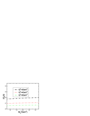
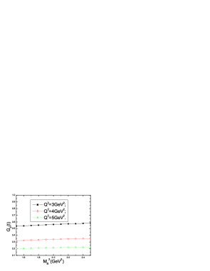
The input parameters have to be specified before the numerical analysis. We choose the suitable range for the Borel parameter $M_{B}$, $1.5GeV^{2}<M_{B}^{2}<2.5GeV^{2}$. In this range, the Borel parameter $M_{B}$ is small enough to warrant the higher mass resonances and continuum states are suppressed sufficiently, on the other hand, it is large enough to warrant the convergence of the light-cone expansion with increasing twists in the perturbative QCD calculation [17, 18]. The numerical results indicate that in this range the form-factors $G_{A}(t=-Q^{2})$ and $G_{P}(t=-Q^{2})$ are almost independent on the Borel parameter $M_{B}$, which we can see from the Fig.1 and Fig.2 respectively for the central values of the eight input parameters $f_{N}$, $\lambda_{1}$, $\lambda_{2}$, $V_{1}^{d}$, $A_{1}^{u}$, $f_{d}^{1}$, $f_{d}^{2}$ and $f_{u}^{1}$.

Figure 1: The axial form-factor $G_{A}(t)$ with the parameter $M_{B}$ for $s_{0}=2.25GeV^{2}$.

Figure 2: The induced pseudoscalar form-factor $G_{P}(t)$ with the parameter $M_{B}$ for $s_{0}=2.25GeV^{2}$.

For simplicity, we choose the standard values for the threshold parameter $s_{0}$, $s_{0}=2.25GeV^{2}$, to subtract the contributions from the higher resonances and continuum states i.e. we restrict the range of integral to the energy region below the Roper resonance ($N(1440)$); furthermore, it is large enough to take into account all contributions from the neutron. For $Q^{2}=(2-9)GeV^{2}$, $x\geq x_{0}=0.5-0.8$, the average value $\langle x\rangle=0.75-0.90$, with the intermediate and large space-like momentum $Q^{2}$, the end-point (soft) contributions (or the Feynman mechanism) are dominant, it is consistent with the growing consensus that the onset of the perturbative QCD region in exclusive processes is postponed to very large energy scales. The parameters in the light-cone distribution amplitudes $\phi_{3}^{0}$, $\phi_{6}^{0}$, $\phi_{4}^{0}$, $\phi_{5}^{0}$, $\xi_{4}^{0}$, $\xi_{5}^{0}$, $\psi_{4}^{0}$, $\psi_{5}^{0}$, $\phi_{3}^{-}$, $\phi_{3}^{+}$, $\phi_{4}^{-}$, $\phi_{4}^{+}$, $\psi_{4}^{-}$, $\psi_{4}^{+}$, $\xi_{4}^{-}$, $\xi_{4}^{+}$, $\phi_{5}^{-}$, $\phi_{5}^{+}$, $\psi_{5}^{-}$, $\psi_{5}^{+}$, $\xi_{5}^{-}$ ,$\xi_{5}^{+}$, $\phi_{6}^{-}$, $\phi_{6}^{+}$ are scale dependent and can be calculated with the corresponding QCD sum rules. They are functions of eight independent parameters $f_{N}$, $\lambda_{1}$, $\lambda_{2}$, $V_{1}^{d}$, $A_{1}^{u}$, $f^{d}_{1}$, $f^{d}_{2}$ and $f^{u}_{1}$, the three parameters $f_{N}$, $\lambda_{1}$ and $\lambda_{2}$ are related to the leading order (or $S$-wave) contributions in the conformal spin expansion, the remaining five parameters $V_{1}^{d}$, $A_{1}^{u}$, $f^{d}_{1}$, $f^{d}_{2}$ and $f^{u}_{1}$ are related to the next-to-leading order (or $P$-wave) contributions in the conformal spin expansion; the explicit expressions are presented in the appendix, for detailed and systematic studies about this subject, one can consult Ref.[13]. Here we take the values at the energy scale $\mu=1GeV$ and neglect the evolution with the energy scale $\mu$ for simplicity, the values for the eight independent parameters are taken as $f_{N}=(5.3\pm 0.5)\times 10^{-3}GeV^{2}$, $\lambda_{1}=-(2.7\pm 0.9)\times 10^{-2}GeV^{2}$, $\lambda_{2}=(5.1\pm 1.9)\times 10^{-2}GeV^{2}$, $V_{1}^{d}=0.23\pm 0.03$, $A_{1}^{u}=0.38\pm 0.15$, $f_{1}^{d}=0.6\pm 0.2$, $f_{2}^{d}=0.15\pm 0.06$ and $f_{1}^{u}=0.22\pm 0.15$. In estimating those coefficients with the QCD sum rules, only the first few moments are taken into account, the values are not very accurate. In the limit $Q^{2}\rightarrow\infty$, the five parameters related to the light-cone distribution amplitudes with the $P$-wave conformal spin take the asymptotic values $f^{d}_{1}=\frac{3}{10}$, $f^{d}_{2}=\frac{4}{15}$, $f^{u}_{1}=\frac{1}{10}$, $A^{u}_{1}=0$ and $V^{d}_{1}=\frac{1}{3}$.

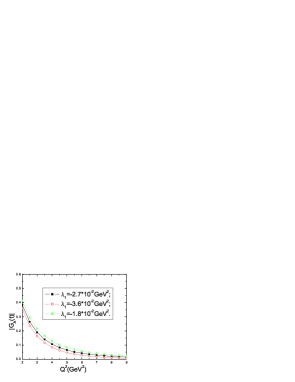
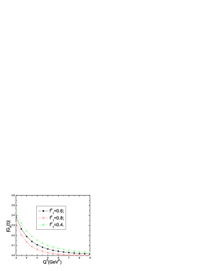
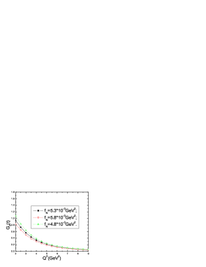
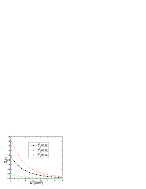
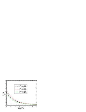
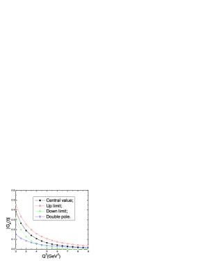
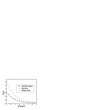
We perform the operator product expansion in the light-cone with large $Q^{2}$ and $P^{\prime 2}$, the form-factors $G_{A}(t=-Q^{2})$ and $G_{P}(t=-Q^{2})$ make sense at the regions, for example, $Q^{2}>2GeV^{2}$, with low momentum transfers, the operator product expansion is questionable. In numerical analysis, we observe that the axial form-factor $G_{A}(t=-Q^{2})$ is sensitive to the two parameters $\lambda_{1}$ and $f^{d}_{1}$, small variations of the two parameters can lead to relatively large changes for the values, the induced pseudoscalar form-factor $G_{P}(t=-Q^{2})$ is sensitive to the four parameters $f_{N}$, $\lambda_{1}$, $f^{d}_{1}$ and $f^{u}_{1}$, small variations of those parameters, especially the $\lambda_{1}$ and $f^{d}_{1}$, can lead to large changes for the values, which are shown in the Fig.3, Fig.4, Fig.5, Fig.6, Fig.7 and Fig.8, respectively. The large uncertainties can impair the predictive ability of the sum rules, the parameters $\lambda_{1}$, $f^{d}_{1}$, $f_{N}$ and $f^{u}_{1}$ should be refined to make robust predictions, in Ref.[10], we observe that the scalar-form factor of the nucleon is sensitive to the four parameters $\lambda_{1}$, $f^{d}_{1}$, $f^{d}_{2}$ and $f^{u}_{1}$, so refining the three parameters $\lambda_{1}$, $f^{d}_{1}$ and $f^{u}_{1}$ is of great importance. The final numerical values for the axial form-factor $G_{A}(t=-Q^{2})$ and induced pseudoscalar form-factor $G_{P}(t=-Q^{2})$ at the intermediate and large space-like momentum regions, $2GeV^{2}<Q^{2}<9GeV^{2}$, are plotted in the Fig.9 and Fig.10 respectively.

From those figures, we can see that the central values of the axial form-factor $G_{A}(t=-Q^{2})$ lie above the results of the double-pole fitted formulation from the neutrino scattering experiments [2],

$$G_{A}(t)=\frac{g_{A}}{(1-t/M_{A}^{2})^{2}}\,,$$ (15)

here we take the values $g_{A}=1.2673$, $M_{A}=1.026$, and neglect the uncertainties for simplicity; at the region $Q^{2}>4.0GeV^{2}$, the values of the double-pole fitted formulation lie between the up and down limits, our results can make both qualitative and quantitative predictions. Furthermore, our results are compatible with the calculation of lattice QCD [19] and chiral quark models [20]. For the induced pseudoscalar form-factor $G_{P}(t=-Q^{2})$, the uncertainties are very large and the values make sense only qualitatively, not quantitatively, our results are compatible with the calculation from the Bethe-Salpeter equation [21].

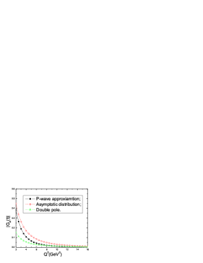
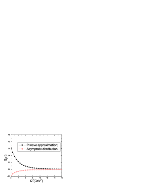
In the limit $Q^{2}\rightarrow\infty$, we present the numerical values for the axial form-factor $G_{A}(t=-Q^{2})$ and the induced pseudoscalar form-factor $G_{P}(t=-Q^{2})$ with the asymptotic light-cone distribution amplitudes in the Fig.11 and Fig.12, respectively. From the Fig.11, we can see that for the axial form-factor $G_{A}(t=-Q^{2})$, the values with the asymptotic light-cone distribution amplitudes lie above the corresponding ones with the light-cone distribution amplitudes in the $P$-wave approximation, at $Q^{2}>10GeV^{2}$, the two curves approach the values of the double-pole fitted formulation $G_{A}(t=-Q^{2})\sim\frac{1}{Q^{4}}$, which is expected from the naive power counting rules. From the Fig.12, we can see that for the induced pseudoscalar form-factor $G_{P}(t=-Q^{2})$, the values with the asymptotic light-cone distribution amplitudes have negative sign comparing with the corresponding ones with the light-cone distribution amplitudes in the $P$-wave approximation, at $Q^{2}>10GeV^{2}$, the two curves approach the same values. The large difference between the values from the asymptotic light-cone distribution amplitudes and the $P$-wave approximated light-cone distribution amplitudes again indicate the importance of the contributions from the $P$-wave conformal spin at the intermediate and large momentum transfers $2GeV^{2}<Q^{2}<10GeV^{2}$, to make robust predictions, we have to refine the five parameters.

The consistent and complete LCSR analysis should take into account the contributions from the perturbative $\alpha_{s}$ corrections, the distribution amplitudes with additional valence gluons and quark-antiquark pairs, and improve the parameters which enter in the LCSRs.

Figure 3: The axial form-factor $G_{A}(t)$ with the parameters $M_{B}^{2}=2.0GeV^{2}$ and $\lambda_{1}$.

Figure 4: The axial form-factor $G_{A}(t)$ with the parameters $M_{B}^{2}=2.0GeV^{2}$ and $f^{d}_{1}$.

Figure 5: The induced pseudoscalar form-factor $G_{P}(t)$ with the parameters $M_{B}^{2}=2.0GeV^{2}$ and $f_{N}$.

Figure 6: The induced pseudoscalar form-factor $G_{P}(t)$ with the parameters $M_{B}^{2}=2.0GeV^{2}$ and $\lambda_{1}$.

Figure 7: The induced pseudoscalar form-factor $G_{P}(t)$ with the parameters $M_{B}^{2}=2.0GeV^{2}$ and $f^{d}_{1}$.

Figure 8: The induced pseudoscalar form-factor $G_{P}(t)$ with the parameters $M_{B}^{2}=2.0GeV^{2}$ and $f^{u}_{1}$.

Figure 9: The axial form-factor $G_{A}(t)$ with the parameter $M_{B}^{2}=2.0GeV^{2}$.

Figure 10: The induced pseudoscalar form-factor $G_{P}(t)$ with the parameter $M_{B}^{2}=2.0GeV^{2}$.

Figure 11: The axial form-factor $G_{A}(t)$ with the parameters $f_{N}=5.3\times 10^{-3}GeV^{2}$, $\lambda_{1}=-2.7\times 10^{-2}GeV^{2}$, $\lambda_{2}=5.1\times 10^{-2}GeV^{2}$ and $M_{B}^{2}=2.0GeV^{2}$.

Figure 12: The $G_{P}(t)$ with the parameters $f_{N}=5.3\times 10^{-3}GeV^{2}$, $\lambda_{1}=-2.7\times 10^{-2}GeV^{2}$, $\lambda_{2}=5.1\times 10^{-2}GeV^{2}$ and $M_{B}^{2}=2.0GeV^{2}$.

4 Conclusion

In this work, we calculate the axial and induced pseudoscalar form-factors $G_{A}(t=-Q^{2})$ and $G_{P}(t=-Q^{2})$ of the nucleons in the framework of the LCSR approach up to twist-6 three valence quark light-cone distribution amplitudes. The form-factors $G_{A}(t=-Q^{2})$ and $G_{P}(t=-Q^{2})$ at intermediate and large momentum transfers with $Q^{2}>2GeV^{2}$ have significant contributions from the end-point (soft) terms. The axial form-factor $G_{A}(t=-Q^{2})$ is sensitive to the two parameters $\lambda_{1}$ and $f^{d}_{1}$, small variations of the two parameters can lead to relatively large changes for the values; the induced pseudoscalar form-factor $G_{P}(t=-Q^{2})$ is sensitive to the four parameters $f_{N}$, $\lambda_{1}$, $f^{d}_{1}$ and $f^{u}_{1}$, small variations of those parameters, especially the $\lambda_{1}$ and $f^{d}_{1}$, can lead to large changes for the values. The large uncertainties can impair the predictive ability of the sum rules, the parameters $\lambda_{1}$, $f^{d}_{1}$, $f_{N}$ and $f^{u}_{1}$ should be refined to make robust predictions. The numerical values for the $G_{A}(t=-Q^{2})$ are compatible with the experimental data and theoretical calculations, for example, chiral quark model and lattice QCD. In the limit $Q^{2}\rightarrow\infty$, the values for the axial form-factor $G_{A}(t=-Q^{2})$ with both the asymptotic light-cone distribution amplitudes and the light-cone distribution amplitudes in the $P$-wave approximation approach the results of the double-pole fitted formulation $G_{A}(t=-Q^{2})\sim\frac{1}{Q^{4}}$. The numerical results for the induced pseudoscalar form-factor $G_{P}(t=-Q^{2})$ are compatible with the calculation from the Bethe-Salpeter equation, in the limit $Q^{2}\rightarrow\infty$, the values of the $G_{A}(t=-Q^{2})$ with both the asymptotic light-cone distribution amplitudes and the light-cone distribution amplitudes in the $P$-wave approximation approach the same values. The consistent and complete LCSR analysis should take into account the contributions from the perturbative $\alpha_{s}$ corrections, the distribution amplitudes with additional valence gluons and quark-antiquark pairs, and improve the parameters which enter in the LCSRs.

Appendix

$$V_{1}(x_{i},\mu) = 120x_{1}x_{2}x_{3}[\phi_{3}^{0}(\mu)+\phi_{3}^{+}(\mu)(1-3x_{3})],$$

$$V_{2}(x_{i},\mu) = 24x_{1}x_{2}[\phi_{4}^{0}(\mu)+\phi_{3}^{+}(\mu)(1-5x_{3})],$$

$$V_{3}(x_{i},\mu) = 12x_{3}\{\psi_{4}^{0}(\mu)(1-x_{3})+\psi_{4}^{-}(\mu)[x_{1}^{2}+x_{2}^{2}-x_{3}(1-x_{3})]$$

$$+\psi_{4}^{+}(\mu)(1-x_{3}-10x_{1}x_{2})\},$$

$$V_{4}(x_{i},\mu) = 3\{\psi_{5}^{0}(\mu)(1-x_{3})+\psi_{5}^{-}(\mu)[2x_{1}x_{2}-x_{3}(1-x_{3})]$$

$$+\psi_{5}^{+}(\mu)[1-x_{3}-2(x_{1}^{2}+x_{2}^{2})]\},$$

$$V_{5}(x_{i},\mu) = 6x_{3}[\phi_{5}^{0}(\mu)+\phi_{5}^{+}(\mu)(1-2x_{3})],$$

$$V_{6}(x_{i},\mu) = 2[\phi_{6}^{0}(\mu)+\phi_{6}^{+}(\mu)(1-3x_{3})].$$

$$A_{1}(x_{i},\mu) = 120x_{1}x_{2}x_{3}\phi_{3}^{-}(\mu)(x_{2}-x_{1}),$$

$$A_{2}(x_{i},\mu) = 24x_{1}x_{2}\phi_{4}^{-}(\mu)(x_{2}-x_{1}),$$

$$A_{3}(x_{i},\mu) = 12x_{3}(x_{2}-x_{1})\{(\psi_{4}^{0}(\mu)+\psi_{4}^{+}(\mu))+\psi_{4}^{-}(\mu)(1-2x_{3})\},$$

$$A_{4}(x_{i},\mu) = 3(x_{2}-x_{1})\{-\psi_{5}^{0}(\mu)+\psi_{5}^{-}(\mu)x_{3}+\psi_{5}^{+}(\mu)(1-2x_{3})\},$$

$$A_{5}(x_{i},\mu) = 6x_{3}(x_{2}-x_{1})\phi_{5}^{-}(\mu)$$

$$A_{6}(x_{i},\mu) = 2(x_{2}-x_{1})\phi_{6}^{-}(\mu).$$

$$T_{1}(x_{i},\mu) = 120x_{1}x_{2}x_{3}[\phi_{3}^{0}(\mu)+\frac{1}{2}(\phi_{3}^{-}-\phi_{3}^{+})(\mu)(1-3x_{3})],$$

$$T_{2}(x_{i},\mu) = 24x_{1}x_{2}[\xi_{4}^{0}(\mu)+\xi_{4}^{+}(\mu)(1-5x_{3})],$$

$$T_{3}(x_{i},\mu) = 6x_{3}\{(\xi_{4}^{0}+\phi_{4}^{0}+\psi_{4}^{0})(\mu)(1-x_{3})+(\xi_{4}^{-}+\phi_{4}^{-}-\psi_{4}^{-})(\mu)[x_{1}^{2}+x_{2}^{2}-x_{3}(1-x_{3})]$$

$$+(\xi_{4}^{+}+\phi_{4}^{+}+\psi_{4}^{+})(\mu)(1-x_{3}-10x_{1}x_{2})\},$$

$$T_{4}(x_{i},\mu) = \frac{3}{2}\{(\xi_{5}^{0}+\phi_{5}^{0}+\psi_{5}^{0})(\mu)(1-x_{3})+(\xi_{5}^{-}+\phi_{5}^{-}-\psi_{5}^{-})(\mu)[2x_{1}x_{2}-x_{3}(1-x_{3})]$$

$$+(\xi_{5}^{+}+\phi_{5}^{+}+\psi_{5}^{+})(\mu)(1-x_{3}-2(x_{1}^{2}+x_{2}^{2}))\},$$

$$T_{5}(x_{i},\mu) = 6x_{3}[\xi_{5}^{0}(\mu)+\xi_{5}^{+}(\mu)(1-2x_{3})],$$

$$T_{6}(x_{i},\mu) = 2[\phi_{6}^{0}(\mu)+\frac{1}{2}(\phi_{6}^{-}-\phi_{6}^{+})(\mu)(1-3x_{3})],$$

$$T_{7}(x_{i},\mu) = 6x_{3}\{(-\xi_{4}^{0}+\phi_{4}^{0}+\psi_{4}^{0})(\mu)(1-x_{3})+(-\xi_{4}^{-}+\phi_{4}^{-}-\psi_{4}^{-})(\mu)[x_{1}^{2}+x_{2}^{2}-x_{3}(1-x_{3})]$$

$$+(-\xi_{4}^{+}+\phi_{4}^{+}+\psi_{4}^{+})(\mu)(1-x_{3}-10x_{1}x_{2})\},$$

$$T_{8}(x_{i},\mu) = \frac{3}{2}\{(-\xi_{5}^{0}+\phi_{5}^{0}+\psi_{5}^{0})(\mu)(1-x_{3})+(-\xi_{5}^{-}+\phi_{5}^{-}-\psi_{5}^{-})(\mu)[2x_{1}x_{2}-x_{3}(1-x_{3})]$$

$$+(-\xi_{5}^{+}+\phi_{5}^{+}+\psi_{5}^{+})(\mu)(1-x_{3}-2(x_{1}^{2}+x_{2}^{2}))\}.$$

$$S_{1}(x_{i},\mu) = 6x_{3}(x_{2}-x_{1})\left[(\xi_{4}^{0}+\phi_{4}^{0}+\psi_{4}^{0}+\xi_{4}^{+}+\phi_{4}^{+}+\psi_{4}^{+})(\mu)+(\xi_{4}^{-}+\phi_{4}^{-}-\psi_{4}^{-})(\mu)(1-2x_{3})\right]\,,$$

$$S_{2}(x_{i},\mu) = \frac{3}{2}(x_{2}-x_{1})\left[-\left(\psi_{5}^{0}+\phi_{5}^{0}+\xi_{5}^{0}\right)(\mu)+\left(\xi_{5}^{-}+\phi_{5}^{-}-\psi_{5}^{0}\right)(\mu)x_{3}\right.$$

$$\left.+\left(\xi_{5}^{+}+\phi_{5}^{+}+\psi_{5}^{0}\right)(\mu)(1-2x_{3})\right]\,,$$

$$P_{1}(x_{i},\mu) = 6x_{3}(x_{2}-x_{1})\left[(\xi_{4}^{0}-\phi_{4}^{0}-\psi_{4}^{0}+\xi_{4}^{+}-\phi_{4}^{+}-\psi_{4}^{+})(\mu)+(\xi_{4}^{-}-\phi_{4}^{-}+\psi_{4}^{-})(\mu)(1-2x_{3})\right]\,,$$

$$P_{2}(x_{i},\mu) = \frac{3}{2}(x_{2}-x_{1})\left[\left(\psi_{5}^{0}+\psi_{5}^{0}-\xi_{5}^{0}\right)(\mu)+\left(\xi_{5}^{-}-\phi_{5}^{-}+\psi_{5}^{0}\right)(\mu)x_{3}\right.$$

$$\left.+\left(\xi_{5}^{+}-\phi_{5}^{+}-\psi_{5}^{0}\right)(\mu)(1-2x_{3})\right]\,.$$

$$\mathcal{V}_{1}^{d}(x_{3}) = \frac{x_{3}^{2}}{24}(\lambda_{1}C_{\lambda}^{d}+f_{N}C_{f}^{d}),$$

$$\mathcal{V}_{1}^{u}(x_{2}) = \frac{x_{2}^{2}}{24}(\lambda_{1}C_{\lambda}^{u}+f_{N}C_{f}^{u}),$$

$$C_{\lambda}^{d} = -(1-x_{3})[11+131\,x_{3}-169x_{3}^{2}+63x_{3}^{3}-30\,f_{1}^{d}\,(3+11x_{3}-17x_{3}^{2}+7x_{3}^{3})]$$

$$-12\,(3-10\,f_{1}^{d})\,\ln x_{3},$$

$$C_{f}^{d} = -(1-x_{3})\,[1441+505x_{3}-3371x_{3}^{2}+3405x_{3}^{3}-1104x_{3}^{4}-24V_{1}^{d}$$

$$(207-3x_{3}-368x_{3}^{2}+412x_{3}^{3}-138x_{3}^{4})]-12(73-220\,V_{1}^{d})\,\ln x_{3},$$

$$C_{\lambda}^{u} = -(1-x_{2})^{3}[13-20f_{1}^{d}+3x_{2}+10f_{1}^{u}(1-3x_{2})],$$

$$C_{f}^{u} = (1-x_{2})^{3}[113+495x_{2}-552x_{2}^{2}+10A_{1}^{u}(-1+3x_{2})$$

$$+2V_{1}^{d}(113-951x_{2}+828x_{2}^{2})].$$

$$\mathcal{A}_{1}^{d}(x_{3}) = 0,$$

$$\mathcal{A}_{1}^{u}(x_{2}) = \frac{x_{2}^{2}}{24}(1-x_{2})^{3}(\lambda_{1}D_{\lambda}^{u}+f_{N}D_{f}^{u}),$$

$$D_{\lambda}^{u} = 29-45x_{2}-10f_{1}^{u}(7-9x_{2})-20f_{1}^{d}(5-6x_{2}),$$

$$D_{f}^{u} = 11+45x_{2}+10V_{1}^{d}(1-30x_{2})-2A_{1}^{u}(113-951x_{2}+828x_{2}^{2}).$$

$$\phi_{3}^{0}=\phi_{6}^{0}=f_{N}\,,\hskip 8.5359pt \phi_{4}^{0}=\phi_{5}^{0}=\frac{1}{2}\left(\lambda_{1}+f_{N}\right)\,,$$

$$\xi_{4}^{0}=\xi_{5}^{0}=\frac{1}{6}\lambda_{2}\,, \psi_{4}^{0}=\psi_{5}^{0}=\frac{1}{2}\left(f_{N}-\lambda_{1}\right)\,.$$

$$\tilde{\phi}_{3}^{-} = \frac{21}{2}A_{1}^{u},$$

$$\tilde{\phi}_{3}^{+} = \frac{7}{2}(1-3V_{1}^{d}),$$

$$\phi_{4}^{-} = \frac{5}{4}\left(\lambda_{1}(1-2f_{1}^{d}-4f_{1}^{u})+f_{N}(2A_{1}^{u}-1)\right)\,,$$

$$\phi_{4}^{+} = \frac{1}{4}\left(\lambda_{1}(3-10f_{1}^{d})-f_{N}(10V_{1}^{d}-3)\right)\,,$$

$$\psi_{4}^{-} = -\frac{5}{4}\left(\lambda_{1}(2-7f_{1}^{d}+f_{1}^{u})+f_{N}(A_{1}^{u}+3V_{1}^{d}-2)\right)\,,$$

$$\psi_{4}^{+} = -\frac{1}{4}\left(\lambda_{1}(-2+5f_{1}^{d}+5f_{1}^{u})+f_{N}(2+5A_{1}^{u}-5V_{1}^{d})\right)\,,$$

$$\xi_{4}^{-} = \frac{5}{16}\lambda_{2}(4-15f_{2}^{d})\,,$$

$$\xi_{4}^{+} = \frac{1}{16}\lambda_{2}(4-15f_{2}^{d})\,,$$

$$\phi_{5}^{-} = \frac{5}{3}\left(\lambda_{1}(f_{1}^{d}-f_{1}^{u})+f_{N}(2A_{1}^{u}-1)\right)\,,$$

$$\phi_{5}^{+} = -\frac{5}{6}\left(\lambda_{1}(4f_{1}^{d}-1)+f_{N}(3+4V_{1}^{d})\right)\,,$$

$$\psi_{5}^{-} = \frac{5}{3}\left(\lambda_{1}(f_{1}^{d}-f_{1}^{u})+f_{N}(2-A_{1}^{u}-3V_{1}^{d})\right)\,,$$

$$\psi_{5}^{+} = -\frac{5}{6}\left(\lambda_{1}(-1+2f_{1}^{d}+2f_{1}^{u})+f_{N}(5+2A_{1}^{u}-2V_{1}^{d})\right)\,,$$

$$\xi_{5}^{-} = -\frac{5}{4}\lambda_{2}f_{2}^{d}\,,$$

$$\xi_{5}^{+} = \frac{5}{36}\lambda_{2}(2-9f_{2}^{d})\,,$$

$$\phi_{6}^{-} = \phantom{-}\frac{1}{2}\left(\lambda_{1}(1-4f_{1}^{d}-2f_{1}^{u})+f_{N}(1+4A_{1}^{u})\right)\,,$$

$$\phi_{6}^{+} = -\frac{1}{2}\left(\lambda_{1}(1-2f_{1}^{d})+f_{N}(4V_{1}^{d}-1)\right)\,.$$

References

- [1] S. L Adler, R. F. Dashen, Current Algebra and Application to Particle Physics (Benjamin, New York, 1968).
- [2] V. Bernard, L. Elouadrhiri, U. G. Meissner, J. Phys. G28 (2002) R1.
- [3] S. Weinberg, Phys. Rev. 112 (1958) 1375.
- [4] M. L. Goldberger, S.B. Treiman, Phys. Rev. 110 (1958) 1178; M. L. Goldberger, S. B. Treiman, Phys. Rev. 111 (1958) 354.
- [5] I. I. Balitsky, V. M. Braun and A. V. Kolesnichenko, Nucl. Phys. B312 (1989) 509; V. L. Chernyak and I. R. Zhitnitsky, Nucl. Phys. B345 (1990) 137; V. L. Chernyak and A. R. Zhitnitsky, Phys. Rept. 112 (1984) 173.
- [6] V. M. Braun, hep-ph/9801222; P. Colangelo and A. Khodjamirian, hep-ph/0010175.
- [7] M. A. Shifman, A. I. Vainshtein and V. I. Zakharov, Nucl. Phys. B147 (1979) 385, 448.
- [8] V. Braun and I. Halperin, Phys. Lett. B328 (1994) 457; V. M. Braun, A. Khodjamirian and M. Maul, Phys. Rev. D61 (2000) 073004.
- [9] V. M. Braun, A. Lenz, N. Mahnke, Phys. Rev. D65 (2002) 074011; A. Lenz, M. Wittmann, E. Stein, Phys. Lett. B581 (2004) 199; V. M. Braun, A. Lenz, G. Peters, A.V. Radyushkin, hep-ph/0510237 .
- [10] Z. G. Wang, S. L. Wan, W. M. Yang, hep-ph/0601025.
- [11] M. Q. Huang, D. W. Wang, Phys. Rev. D69 (2004) 094003.
- [12] V. L. Chernyak and I. R. Zhitnitsky, Nucl. Phys. B246 (1984) 52; I. D. King and C. T. Sachrajda, Nucl. Phys. B279 (1987) 785; V. L. Chernyak, A. A. Ogloblin and I. R. Zhitnitsky, Sov. J. Nucl. Phys. 48 (1988) 536; Z. Phys. C 42 (1989) 583.
- [13] V. Braun, R. J. Fries, N. Mahnke and E. Stein, Nucl. Phys. B 589 (2000) 381; Erratum-ibid. B607 (2001) 433.
- [14] G. P. Lepage and S. J. Brodsky, Phys. Rev. Lett. 43 (1979) 545, 1625 (E); V. A. Avdeenko, V. L. Chernyak and S. A. Korenblit, Yad. Fiz. 33 (1981) 481; S. J. Brodsky, G. P. Lepage and A. A. Zaidi, Phys. Rev. D23 (1981) 1152; S. J. Brodsky and G. P. Lepage, A. I. Milshtein and V. S. Fadin, Yad. Fiz. 35 (1982) 1603.
- [15] I. I. Balitsky and V. M. Braun, Nucl. Phys. B311 (1989) 541.
- [16] M. Diehl, T. Feldmann, R. Jakob and P. Kroll, Eur. Phys. J. C8 (1999) 409.
- [17] B. L. Ioffe and A. V. Smilga Nucl. Phys. B232 (1984) 109 ; I. I. Balitsky and A. V. Yung, Phys. Lett. B129 (1983) 328.
- [18] B. L. Ioffe, Nucl. Phys. B188 (1981) 317; Erratum-ibid. B191 (1981) 591.
- [19] S. J. Dong, J. F. Lagae, K. F. Liu, Phys. Rev. D 54 (1996) 5496 .
- [20] A. Silva, H. C. Kim, D. Urbano, K. Goeke, Phys. Rev. D72(2005) 094011; K. Khosonthongkee, V. E. Lyubovitskij, Th. Gutsche, A. Faessler, K. Pumsa-ard, S. Cheedket, Y. Yan, J. Phys. G30 (2004) 793;
- [21] G. Hellstern. R. Alkofer, M. Oettel, H. Reinhardt, Nucl. Phys. A627 (1997) 679.