Classical Cancellation of the Cosmological Constant Re-Considered

Abstract

We revisit a scenario in which the cosmological constant is cancelled by the potential energy of a slowly evolving scalar field, or “cosmon”. The cosmon’s evolution is tied to the cosmological constant by a feedback mechanism. This feedback is achieved by an unconventional coupling of the cosmon field to the Ricci curvature scalar. The solutions show that the effective cosmological constant evolves approximately as $t^{-2}$ and remains always of the same order as the density of ordinary matter and radiation. Newton’s constant varies on cosmological time scales, with $\dot{G}_{N}/G_{N}\ll 1/t$. $G_{N}$ could have been somewhat different, and possibly smaller, at the time of Big Bang nucleosynthesis.

1 Introduction

Many ideas have been suggested for solving the cosmological constant problem review , but none so far has proven to be completely satisfactory. An old idea is that the vacuum energy of ordinary fields is cancelled by some compensating field, sometimes called a “cosmon”. The cosmon would roll down a potential hill until it had lowered the total vacuum energy to an acceptable level barr ; ford ; cosmon . The question is how the cosmon field would “know” when to stop rolling. If the cosmon potential happened to have a minimum at exactly the right height, it can cancel off other contributions to $\Lambda$. However, that would obviously be nothing other than a manual setting of the total $\Lambda$ to zero at the minimum, i.e. just the old fine-tuning of $\Lambda$ that one is trying to avoid.

If a conspiracy of parameters is to be avoided, it is imperative that the cosmon action does not directly depend on the contributions to $\Lambda$ coming from other sectors of the theory. But how, in that case, is the cosmon to know when to stop rolling? Some sort of feedback mechanism is required. Several such mechanisms have been proposed over the years barr ; ford ; cosmon ; feedback . The one we will explore in this paper was proposed in the papers of Ref. barr ; ford in the mid 1980s, and is based on the idea that the cosmon field couples to the scalar curvature $R$. Since the trace of the Einstein field equations tells us that $-R=2\Lambda+\frac{1}{2}(\rho-3p)$, the cosmon can learn about $\Lambda$ through its effect on $R$. The conventional wisdom, based on a “no-go theorem” stated in Weinberg’s well-known 1989 review of the cosmological constant problem, is that this kind of feedback mechanism cannot work. However, this “theorem”, which originally comes from the papers barr ; ford , does not apply to the kind of model we discuss in this paper, as we shall see. (Note: we will be using units where $16\pi G_{N}=1$, signature -+++, and the sign convention in which a sphere has negative $R$.)

Before exploring this idea further, there is a general point that may be important. In any realistic feedback mechanism, it would seem that the “effective vacuum energy” $\lambda$ — by which we mean the vacuum energy from other sectors of the theory ($\Lambda$) plus the potential energy in the cosmon field ($V_{cosmon}$) — must fall to zero as time passes in such a way that it is always of roughly the same order as the matter energy density, $\rho_{matter}$. By “matter” here we mean all forms of particles, including baryons, photons, neutrinos, dark matter particles, etc. The reason for this is as follows. If $\lambda$ falls off significantly more slowly than $\rho_{matter}$, then it will quickly come to dominate the universe, which will end up with $\Omega_{matter}$ being negligibly small. If, on the other hand, $\lambda$ falls off significantly faster than $\rho_{matter}$, then very early in the history of the universe the effective cosmological constant would be much smaller than $T^{4}$, where $T$ is the temperature of the universe. However, that would mean that any subsequent phase transition (such as one associated with the symmetry breaking of grand unification, the weak interactions, or the chiral symmetry of the quarks) would drive $\lambda$ very negative, since it would lower $\Lambda$ by an amount of order $T^{4}$. Given the arguments of Coleman and De Luccia coleman and more recently from a string theoretic viewpoint, Banks banks , it is questionable whether such a transition could occur. But if it did, once the universe has negative $\lambda$, it is not clear how it could get out of that hole, as it would have to in order to be consistent with present observations.

The upshot is that any successful feedback mechanism would seem to require that the hidden energy density of $\Lambda$ plus “cosmon” field energy must be roughly of order the density of ordinary matter at all times. This is very suggestive, given the puzzling fact that a dark energy has been observed that is comparable to the matter energy today.

The feedback model we discuss does indeed have the desired feature that $\lambda\sim\rho_{matter}$ at all times. As we shall see, however, this does not necessarily account for the dark energy that has been observed. The problem is that any mechanism that is designed to erase $\Lambda$ will tend to erase dark energy too. In the model we discuss there is indeed energy that is “dark” (namely $\lambda=\Lambda+V_{cosmon}$), which generally falls to zero roughly as $t^{-2}$ and has $w\cong 1/3$. However, after a phase transition $\lambda$ tends to fall more slowly for a period of time, so that $w$ can be smaller than $1/3$ and perhaps even close to $-1$. It is possible that this fact can be used to account for the nearly constant dark energy that has recently been observed.

To return to the specific idea that the feedback occurs through coupling of the cosmon to the scalar curvature $R$, the obvious way for this to happen is through the cosmon potential. To illustrate how this might work, consider a toy model barr ; ford with $V_{cosmon}=-\alpha\phi R$, where $\phi$ always denotes the cosmon in this paper. The effective vacuum energy, as we defined it above, is then $\lambda=\Lambda-\alpha\phi R$. As the cosmon rolls down its linear potential hill, $\lambda$ will decrease; and as that happens, the scalar curvature will decrease as well. This decrease of the scalar curvature reduces the slope ($-\alpha R$) of the cosmon potential, and therefore the cosmon rolling will decelerate (since there is friction due to the Hubble expansion). If we assume that $R$ receives contributions only from $\lambda$, then as $\lambda$ approaches zero, the slope of the cosmon potential will approach zero also, and the velocity of the cosmon’s rolling will approach zero. In other words, whatever the value of $\Lambda$ is, the quantity $\lambda$ will asymptotically approach zero as time passes. That is, the potential energy of the cosmon, $-\alpha\phi R$ will progressively erase $\Lambda$.

In fact, this is what actually would happen in this toy model, as an explicit solution of the field equations shows. Unfortunately, however, Newton’s constant $G_{N}$ suffers a disaster. Instead of the usual Einstein-Hilbert action $-R$, one has $-(1-\alpha\phi)R$. Since the quantity $\alpha\phi R_{U}$ (where $R_{U}$ is the background scalar curvature of the universe) is asymptotically approaching $\Lambda$, that means that $(16\pi G_{N})_{eff}^{-1}=1-\alpha\phi$ is asymptotically approaching $1-\Lambda/R_{U}$, which is exponentially large at present ($\sim 10^{120}$). In other words, Newton’s “constant” turns off in a drastic way.

This is the problem that seems to afflict any attempt to construct a feedback mechanism through a coupling of the cosmon to the scalar curvature through the cosmon potential. (This is the conclusion that was reached in the papers barr ; ford and repeated in Weinberg’s 1989 review review .) This led to an attempt in barr to achieve a viable feedback through the kinetic term of the cosmon. What is required is that negative powers of $R$ appear in the cosmon kinetic term, which, of course, is a peculiar thing indeed overR . Nevertheless, a model that erases the cosmological constant without any fine-tuning of parameters at the classical level can easily be constructed as shown in barr . In the paper we correct and extend the analysis in that earlier paper, and address several important issues that were not considered there.

This paper is organized as follows. In section 2 we present the toy model that we are discussing and find cosmological solutions for the cases where cosmon energy is dominant and where radiation is dominant. (In barr only the cosmon-dominated case was considered, and the analysis of it was faulty, since certain assumptions were made that were not self-consistent.) We also discuss the stability of the solutions, and what the cosmon equation of state looks like. We find that while there are modifications to the effective Newton’s constant (because of the appearance of $R$ in the cosmon kinetic term), they are of order 1 and harmless.

In section 3, we look at what happens when baryonic matter (or other matter whose stress-energy tensor is not traceless) is present. We confirm the conclusion of barr that this does not disturb the feedback mechanism for erasing the cosmological constant. However, there is an interesting effect: the cosmon field does wipe out the trace of the stress-energy tensor inside baryonic matter (contrary to what was claimed in barr ). That is, inside a lump of baryonic matter (e.g. a nucleon, atomic nucleus, or neutron star) the cosmon field has a pressure and density such that the total stress-energy tensor is traceless. However, this has less dramatic effects than one might suppose. This will be analyzed in section 3.

In section 4, we discuss other issues, such as stability of solutions, what happens if the vacuum energy is suddenly reset by a phase transition, and quantum corrections to the model and fine-tuning.

In the Appendix we point out certain mistakes and deficiencies in the analysis in barr .

2 The Toy Model

The model that we shall discuss in the rest of this paper has the action

$${\cal L}=-\frac{c^{2}}{2}(\partial_{\sigma}\phi\partial^{\sigma}\phi)R^{-2}+\alpha\phi-R-\Lambda_{0}+{\cal L}_{matter},$$ (1)

where $c$ is a parameter with dimensions of $M^{4}$ that we take to be of order one in Planckian units. $\Lambda_{0}$ is the vacuum energy that we are trying to erase. (It may change suddenly if there is a first order phase transition.) The third term is just the usual Einstein-Hilbert action. Our metric signature is $(-+++)$. We use the convention that $R$ is negative for a sphere.

The idea is the following. As the cosmon rolls down its potential hill, the effective vacuum energy $\lambda=\Lambda_{0}-\alpha\phi$ will decrease, causing $-R$ to decrease also. This in turn will cause the kinetic term of the cosmon to stiffen, so that the rolling of the cosmon will slow down. As $R$ approaches zero, so does the velocity of the cosmon. In fact, even though $R$ approaches zero, $\dot{\phi}$ approaches zero faster, so that the kinetic energy of $\phi$ becomes smaller, not larger, even though $R$ is in the denominator. Our explicit solutions will show this.

Having a negative power of $R$ in the cosmon kinetic term overR can be avoided if we use an auxiliary field:

$$\begin{array}[]{cl}{\cal L}=&-\frac{1}{2}X^{2}(\partial_{\sigma}\phi\partial^{\sigma}\phi)+\alpha\phi\\ &\\ &+(\partial_{\sigma}X\partial^{\sigma}X)/X^{m}-bR(XR-c)^{2}\\ &\\ &-R-\Lambda_{0}+{\cal L}_{matter}.\end{array}$$ (2)

The power $m$ in the kinetic term of the auxiliary field $X$ must be large enough so that $X$ can adjust rapidly to changes in $R$. For large $b$ and $m$ this version of the model reduces to that in Eq. (1). We shall therefore use Eq. (1).

The gravity equation coming from Eq. (1) is

$$\begin{array}[]{ccl}G^{\lambda\rho}(1-f)&=&-\frac{1}{2}T^{\lambda\rho}_{matter}+\frac{1}{2}\lambda g^{\lambda\rho}\\ &&\\ &-&\frac{c^{2}}{2}(\partial^{\lambda}\phi\partial^{\rho}\phi-\frac{3}{2}\partial^{\sigma}\phi\partial_{\sigma}\phi g^{\lambda\rho})R^{-2}\\ &&\\ &+&(g^{\lambda\rho}\Box-\nabla^{(\lambda}\nabla^{\rho)})f,\end{array}$$ (3)

where

$$f\equiv c^{2}\partial^{\sigma}\phi\partial_{\sigma}\phi R^{-3},$$ (4)

and

$$\lambda\equiv\Lambda_{0}-\alpha\phi,$$ (5)

which implies, of course, that $\dot{\lambda}=-\alpha\dot{\phi}$. The last term in Eq. (3) arises from $\frac{\delta R}{\delta g_{\lambda\rho}}\frac{\delta}{\delta R}\left(-\frac{c^{2}}{2}\partial_{\sigma}\phi\partial^{\sigma}\phi R^{-2}\right)=(\delta R/\delta g_{\lambda\rho})f$ after two integrations by parts. As we shall see, when there is only cosmon energy, the combination of fields that we have called $f$ ends up being simply a constant, so that the last term in Eq. (3) vanishes. When there is matter present, however, $f$ is not constant and the last term in Eq. (3) becomes very important, as we shall see.

If we take the trace of Eq. (3), we get

$$\begin{array}[]{l}-R(1+\frac{3}{2}f)=-\frac{1}{2}T_{matter}+2\lambda+3\Box f.\end{array}$$ (6)

The equation of motion for $\phi$ is

$$-\frac{1}{\sqrt{-g}}\partial_{\sigma}\left[\sqrt{-g}(c^{2}\partial^{\sigma}\phi R^{-2})\right]=\alpha,$$ (7)

and assuming a flat Friedmann-Robertson Walker (FRW) ansatz for the metric, the expression for the scalar curvature in terms of the scale factor of the universe $a(t)$ is, with our sign conventions,

$$-R=6\left(\frac{\ddot{a}}{a}+\left(\frac{\dot{a}}{a}\right)^{2}\right).$$ (8)

We will solve these equations first in the case where there is no ordinary matter, but only cosmon energy. Let us assume that $a(t)\propto t^{n}$ and that the fields are constant in space. Then the cosmon equation of motion becomes $t^{-3n}\partial/\partial t\left[t^{3n}\dot{\lambda}R^{-2}\right]=-\alpha^{2}/c^{2}$, and has the solution

$$\begin{array}[]{l}\dot{\lambda}R^{-2}=-\frac{1}{3n+1}(\alpha^{2}/c^{2})t-kt^{-3n}.\end{array}$$ (9)

The second term on the right is a transient that dies off rapidly. (It has already implicitly been assumed to be negligible, since its presence would cause the scale factor to deviate from a pure power dependence on $t$.) It is easily shown that the solution to the coupled equations gives $R$ proportional to $\lambda$, so we will write $-R=2\gamma\lambda$, with the number $\gamma$ to be determined. Substituting this into Eq. (9) and dropping the transient term gives $\lambda=\frac{3n+1}{2\gamma^{2}}(c^{2}/\alpha^{2})t^{-2}$, for large $t$ t2 . From this, it is easy to see that $f$ is independent of $t$, so that the last term in Eq. (6) may be dropped. Since we are assuming that there is no matter present, that equation then takes the simple form $-R(1+\frac{3}{2}f)=2\lambda$, which implies that $(1+\frac{3}{2}f)=\gamma^{-1}$. We can get another relation between $f$ and $\gamma$ from the definition of $f$, Eq. (4), which we can write as $f=(2\gamma)^{-3}(c^{2}/\alpha^{2})\dot{\lambda}^{2}\lambda^{-3}$. Substituting our solution for $\lambda$ into this gives $f=(3n+1)^{-1}\gamma^{-1}$. Combining the two expressions relating $f$ and $\gamma$ gives $\gamma=\frac{6n-1}{2(3n+1)}$ and $f=\frac{2}{6n-1}$. Therefore

$$\begin{array}[]{l}\lambda=\frac{2(3n+1)^{3}}{(6n-1)^{2}}\frac{c^{2}}{\alpha^{2}}t^{-2}.\end{array}$$ (10)

It remains to use Eq. (8), which tells us that $-R=12n(n-\frac{1}{2})t^{-2}$. Our solution for $\lambda$ and $\gamma$ gives $-R=2\gamma\lambda=\frac{2(3n+1)^{2}}{6n-1}\frac{c^{2}}{\alpha^{2}}t^{-2}$. Combining these gives the power $n$ in terms of the parameters of the model:

$$\frac{6n(6n-1)(n-\frac{1}{2})}{(3n+1)^{2}}=\frac{c^{2}}{\alpha^{2}}.$$ (11)

Note that physical quantities must depend on the combination $c^{2}/\alpha^{2}$ since it is invariant under rescalings of the fields. Let us call this combination $\epsilon$. If we take $\epsilon\ll 1$, then

$$\begin{array}[]{l}n\cong\frac{1}{2}+\frac{25}{24}\epsilon.\end{array}$$ (12)

Note that the universe expands faster than $t^{1/2}$. If there is a small amount of radiation in this cosmon-dominated universe, it will redshift as $\rho_{rad}\sim t^{-2-\frac{25}{6}\epsilon}$, whereas the “effective vacuum energy”, $\lambda$, goes as $t^{-2}$. We shall find that the same is true in a radiation dominated universe with a small amount of cosmon energy: the cosmon/radiation ratio grows as a power of $t$, where the power is of order $\epsilon$. Thus if $\epsilon\sim 10^{-2}$, say, the cosmon energy tracks the radiation density very well over many orders of magnitude in time.

The quantity $\lambda$ contains the vacuum energy $\Lambda_{0}$ (i.e. the underlying cosmological constant) and the cosmon potential energy. If one considers the full “dark” stress energy, which includes the contributions from $\Lambda_{0}$ and from both the kinetic and potential energy of the cosmon, one finds that for $\epsilon\ll 1$, $p\cong\rho/3$. In other words, all the “dark” energy — cosmological constant plus cosmon — has an equation of state similar to radiation.

What can we say about Newton’s constant? The coefficient of the Einstein tensor in Eq. (3), which we may call $(16\pi G_{N})_{eff}^{-1}$, is given by $(1-f)=6(n-\frac{1}{2})/(6n-1)$, which for small $\epsilon$ is approximately $\frac{25}{8}\epsilon$. What matters, of course, is not the particular value of $(G_{N})_{eff}$, which is just a meaningless rescaling of the Planck scale, but how $(G_{N})_{eff}$ changes with time. We see that if only cosmon energy (including $\Lambda$) is present $(G_{N})_{eff}$ is constant. We shall see shortly that when matter is present, $(G_{N})_{eff}$ changes over cosmological time scales, but very little if $\epsilon\ll 1$, which is the case of interest.

Now let us turn to the case of a radiation-dominated universe, with some cosmon energy. Since radiation is dominant, one expects the scale factor to grow approximately as $t^{1/2}$, so we take

$$a(t)=a_{0}(t/t_{0})^{1/2}(1+g_{1}(t/t_{0})^{d}+g_{2}(t/t_{0})^{2d}+...),$$ (13)

where $t_{0}$ is some time that, as we shall see, is close to when the cosmon energy is equal to the radiation energy. The power $d$ is negative, as is $g_{1}$, so that the cosmon/radiation ratio decreases. However, since $d$ turns out to be of $O(\epsilon)$, the cosmon/radiation ratio will change very slowly for small $\epsilon$. Eq. (13) gives

$$-R=6d(1+d)g_{1}t_{0}^{-2}(t/t_{0})^{-2+d}+O(t^{-2+2d}).$$ (14)

It is easy to show that the leading behavior of $\lambda$ is $t^{-2+2d}$, so we write

$$\lambda=\lambda_{0}t_{0}^{-2}(t/t_{0})^{-2+2d}+O(t^{-2+3d}).$$ (15)

Substituting Eqs. (14) and (15) into the cosmon equation of motion, Eq. (7), we find $\lambda_{0}=\frac{36}{5}\frac{\alpha^{2}}{c^{2}}\frac{d^{2}(1+d)^{2}}{1-d}g_{1}^{2}$. Substituting Eqs. (14) and (15) into the Eq. (4) (the definition of $f$), we find $f=\frac{24}{25}d(1+d)(\alpha^{2}/c^{2})g_{1}(t/t_{0})^{d}$ to leading order.

Considering now the trace of the gravity equation, Eq. (6), we see that the leading terms on both sides go as $t^{-2+d}$. If we match only the leading terms (which is good enough for our purposes), we may neglect $\lambda$, which contains only terms of order $t^{-2+2d}$ and higher. We may also neglect the $\frac{3}{2}f$ on the left-hand side for the same reason. Since the matter is assumed to be radiation, $T_{matter}=0$. With fields assumed to be constant in space, we need keep only time derivatives, so that Eq. (6) reduces finally to the simple form $-R=-3(\frac{\partial^{2}}{\partial t^{2}}+\frac{3}{2t}\frac{\partial}{\partial t})f=-3d(d+\frac{1}{2})ft^{-2}$, which gives $-R=-\frac{72}{25}d^{2}(d+\frac{1}{2})(1+d)(\alpha^{2}/c^{2})g_{1}t_{0}^{-2}(t/t_{0})^{-2+d}$. Combining this with Eq. (14) yields

$$\begin{array}[]{l}-\frac{6}{25}d(1+2d)=\frac{c^{2}}{\alpha^{2}}=\epsilon.\end{array}$$ (16)

For small $\epsilon$, $d\cong-\frac{25}{6}\epsilon$, so that

$$\lambda/\rho_{radiation}\sim t^{-\frac{25}{3}\epsilon}.$$ (17)

In fact, since the leading term in Einstein’s equations gives $\rho_{radiation}\cong\frac{3}{2}t^{-2}$, one has $\lambda/\rho_{radiation}\cong\lambda_{0}(t/t_{0})^{2d}$. The preceding calculations give the result $\lambda_{0}=-\frac{30d(1+d)^{2}}{(1-d)(1+2d)}g_{1}^{2}$. Consequently, for small $\epsilon$, one has $\lambda/\rho_{radiation}\cong\frac{250}{3}\epsilon g_{1}^{2}(t/t_{0})^{2d}$. We see, then, that when $\lambda$ is comparable to the radiation density, the terms in $a(t)$ of higher order in $t^{d}$ are of the same size as the lower order terms, and the whole approximation scheme we have been using breaks down, as one would indeed have expected.

Note that the effective Newton’s Constant in an era where radiation dominates is (for small $\epsilon$) given by $(16\pi G_{N})_{eff}^{-1}=1-f\cong 1+4g_{1}(t/t_{0})^{-\frac{25}{6}\epsilon}$. That is, $G_{N}$ decreases very slowly, with $\dot{G_{N}}/G_{N}\sim O(\epsilon)/t$ (although see the discussion in Sec. 4 below).

3 What Happens Inside Matter

The mechanism we have been describing relies on the fact that the scalar curvature is a “proxy” for the vacuum energy. However, inside a matter distribution there is also a contribution from the trace of the matter stress-energy, as shown in Eq. (6). One might worry that this would interfere with the mechanism for cancelling the cosmological constant.

To study this situation, let us consider a spherical mass of radius $r_{m}$, and constant density $\rho_{m}$, surrounded by a vacuum. We take $\rho_{m}$ to be nuclear density, for specificity, and the pressure to be negligible. This mass could be a baryon, or a neutron star, for example. One might suppose that since in natural gravitational units, $\rho_{m}\sim 10^{-80}$ while $\lambda\sim 10^{-120}$, that $\rho_{m}$ would dominate the right-hand side of Eq. (6). Let us make this assumption to start with, even though it will prove to be false, because it will be instructive and point us toward the right solution.

Using spherical symmetry, we can write the equation of motion for the cosmon inside the mass as $\frac{1}{r^{2}}\frac{\partial}{\partial r}(r^{2}\frac{\partial\lambda}{\partial r})=\frac{1}{4}\rho_{m}^{2}(\alpha^{2}/c^{2})$. This has the solution, $\lambda=\lambda_{vac}+\frac{1}{24}\rho_{m}^{2}(\alpha^{2}/c^{2})(r^{2}-r_{m}^{2})$, for $r\leq r_{m}$, where $\lambda_{vac}$ is the value of $\lambda$ in the vacuum, which we have given in Eq. (10). Then $\Delta\lambda\equiv\lambda(r=0)-\lambda_{vac}\sim\rho_{m}^{2}r_{m}^{2}$. If $r_{m}$ is the radius of a baryon, this is of order $10^{-120}$ in natural units. Even if $r_{m}$ is the radius of a neutron star, $\Delta\lambda$ is only of order $10^{-80}$. Now consider the quantity $f$. Inside the sphere of matter, $f\cong\frac{c^{2}}{\alpha^{2}}(\frac{\partial\lambda}{\partial r})^{2}R^{-2}\sim\rho_{m}^{2}r_{m}^{2}$, which for a baryon is $O(10^{-120})$ and for a neutron star is $O(10^{-80})$. If our assumptions were correct, then, it would imply that $f\cong 1$ far from the matter and $f\ll 1$ inside. But this cannot be the case, for then somewhere inside or near the matter distribution the quantity $\nabla^{2}f$ would have to be of order $1/r_{m}^{2}$. For a baryon this is $O(10^{-40})$ which is many orders of magnitude larger than nuclear density. That is, the last term in Eq. (6) would greatly dominate, contrary to our assumption. Thus the assumption that $\rho_{m}$ dominates is false.

This shows what the real solution of the coupled equations must look like. It must be that $f=f_{vac}+\tilde{f}(x^{\mu})$, where $\tilde{f}\ll f_{vac}\ll 1$ and $\nabla^{2}\tilde{f}\cong-\frac{1}{6}\rho_{m}$ (inside matter) so that the terms $-\frac{1}{2}T_{matter}$ and $3\Box f$ on the right-hand side of Eq. (6) cancel. Then $-R$ can have the same value inside and outside the matter distribution, allowing $\lambda$ to be nearly spatially constant. Consequently, $f\cong f_{vac}$ even inside matter. This is the only way to get a self-consistent solution.

The net result is the following. The effective Newton’s constant $(16\pi G_{N})_{eff}^{-1}=1-f$ is the same everywhere, both inside baryonic matter (or any other kind of matter) and in the vacuum. This is what we would expect anyway from the Equivalence Principle. However, something very strange happens; namely the total stress energy tensor acts like radiation, since the sum of the matter stress energy and the last term in Eq. (3), namely $(g^{\lambda\rho}\Box-\nabla^{(\lambda}\nabla^{\rho)})f$, gives something traceless. It is easy to see that if the mass of a ball of baryonic matter is $M$ due to $T^{\lambda\rho}_{matter}$, the total mass including the last term in Eq. (6) is only $\frac{2}{3}M$.

Isn’t it catastrophic to have the total stress energy be traceless, even for ordinary matter? For example, consider a box of gas. The spatial average of the pressure inside the box would be $\frac{1}{3}\rho_{gas}$, where $\rho_{gas}$ includes the rest energy of the gas molecules. However, it must be realized that this average pressure is almost all coming from pressure in the cosmon field inside the material particles. The actual gas pressure due to particles colliding with each other is just what would be given by the kinetic theory of gases. On the other hand, the box of gas would gravitate as though it had traceless stress energy.

4 Other Issues

The cosmological solutions we have found are stable under small perturbations. This can be seen from the solution to the cosmon equation of motion given in Eqs. (9) and (10). The first integral of the equation of motion depends on an integration constant denoted $k$ in Eq. (9). One sees that $k$ describes a transient term that dies away with increasing $t$. The integration of Eq. (9) gives another integration constant that we have not shown in Eq. (10). However, the exact solution approaches the one given in Eq. (10) for large $t$.

There is a simple physical reason why the solutions we have given are stable under small perturbations. Imagine that $\lambda$ finds itself at some $t$ with a somewhat smaller value than that given in Eq. (10). Then $R$ will also be somewhat smaller than in our solutions. That will cause the kinetic term of the cosmon to be more “stiff”, which causes the cosmon field to roll down its potential hill more slowly than it does in our solution. In other words, if $\lambda$ is initially ”too small”, it compensates by decreasing more slowly, until eventually it rejoins the asymptotic solution given in Eq. (10). In the same way if $\lambda$ starts off somewhat larger than the solution in Eq.(10), then $R$ is larger and the cosmon rolls down its hill faster until it rejoins the asymptotic solution.

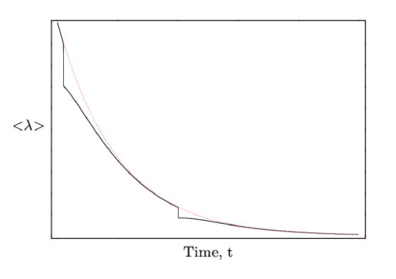
Figure 1: Schematic diagram of the evolution of the cosmon field in the presence of phase transitions. The solid line represents the actual evolution of the cosmon field while the dashed line is the trajectory it would assume in the absence of any phase transitions. In the above case, we have included only two phase transitions; after both of which, the vev of the cosmon field asymptotes back to the pre-phase transition trajectory.

This feature has an important consequence that would be helpful in making a realistic model of cosmology. In a realistic particle theory there would be phase transitions that change the vacuum energy density relatively suddenly, such as those connected with the breaking of grand unified symmetries, supersymmetry, the weak interaction symmetries, or the chiral symmetries of the quarks. Thus, the cosmological “constant” $\Lambda_{0}$ that has to be cancelled off by any cosmon field undergoes sudden jumps downward. The stability of our solutions allows our mechanism to accomodate these jumps. Suppose that $\lambda\equiv\Lambda_{0}-\alpha\phi$ is evolving as shown in Eq. (10), namely as $t^{-2}$, and suddenly a phase transition resets $\Lambda_{0}$ to be smaller by an amount of order $T^{4}$, where $T$ is the temperature at which the phase transition happens. Now $\lambda$ is of order $\rho_{radiation}$, as we have seen; and $\rho_{radiation}$ is of order $T^{4}$. So $\lambda$ will be reset downward by an amount that is of order its own size. Let us suppose that it is not driven to a negative value by this, but only to a smaller positive value. Then, for the reasons we have just explained, the rolling of the cosmon down its hill will be slowed until $\lambda$ rejoins the asymptotic solution we have found. In fact, this could happen repeatedly at various epochs in the history of the universe: the effective vacuum energy could be repeatedly reset by phase transitions, and then after a few e-foldings in time, rejoin its asymptotic solution. Fig.1 schematically illustrates the evolution of just such a cosmon field that undergoes several phase transitions. The fact that $\lambda$ levels off for a period of time after a phase transition and acts more like a cosmological constant may be a possible explanation of the observed dark energy if the universe has recently undergone a phase transition. There is a complication that such an explanation would face, namely that the radiation released in the phase transition would tend to dominate over $\lambda$ for a period of time. How $\lambda$ and $w$ would behave after a phase transition is something that has to be more carefully studied numerically before one can tell if this is a viable explanation of dark energy.

Another effect of the phase transition would be a transient time dependence of $G_{N}$. Suppose that $\Lambda_{0}$ and therefore $R$ is decreased suddenly (compared to t), then by the equation of motion, Eq. 7, one expects $\dot{\phi}R^{-2}$ to be approximately constant during this sudden decrease in R. Thus, $f=-c^{2}\dot{\phi}^{2}R^{-3}$ is driven to a smaller value than the asymptotic solution. As $\lambda$ evolves to a rejoin the asymptotic solution, $f$ will be increasing and hence so will $G_{N}$. In other words, if we are in an era where $\lambda$ is “recovering” from a phase transition (which might explain the near constancy of $\lambda$), then $G_{N}$ might be slowly increasing. This can have implications for Big Bang Nucleosynthesis.

It should be noted that if a phase transition were to drive $\lambda$ negative, there would be a catastrophe: $\lambda$ could not ever become positive again. Rather it would roll to ever more negative values, which would make $|R|$ larger and the cosmon kinetic term less stiff, so that the rolling would accelerate and $\lambda$ would plunge ever faster into the abyss. However, there does not seem to be any reason why phase transitions would necessarily have to drive $\lambda$ negative. Whether or not one did so would depend on the parameters of the theory.

There are of course many other issues that would have to be examined to see if a realistic cosmology could emerge from the toy model we have described or some similar model. We intend to return to these in the future. Another very important issue is whether the kind of theory we are describing could make sense at the quantum level. One obvious issue is whether there is any fine-tuning is involved in the choice of cosmon kinetic term we have made. If one considers the effects of either matter loops or cosmon loops, these do not seem to raise any problems of fine tuning (though we have not proved this). One thing that helps in this regard is that the cosmon only couples to gravity. However, simple power-counting arguments suggest that graviton loops induce a term of the form $(\partial\phi)^{2}/R^{3}$ in addition to $(\partial\phi)^{2}/R^{2}$. The former term would overwhelm the latter unless its coefficient were tuned to be less than about $10^{-120}$, i.e. about the same tuning that is involved in the cosmological constant problem itself. However, even if this is the case, that does not mean that the model achieves nothing. It seems to be a solution to the cosmological constant problem at the classical level (whether a realistic one or not, that remains to be seen). That is, it can solve the “small number problem” even if it does not solve the “fine tuning problem”. However, any conclusions about the quantum theory are premature, as we have not studied it in detail.

5 Conclusions

We have analyzed a toy model that realizes the idea of a feedback mechanism for cancelling the cosmological constant at the classical level. The model has several appealing features. First, the total “dark energy” of vacuum energy plus cosmon field energy is always of the same order as the energy in radiation and matter. This is certainly suggestive, given the observed “cosmic coincidence” that the dark energy is currently of the same order as the energy in particles. Second, the mechanism works even if there are several phase transitions throughout the history of the universe that reset the cosmological constant. As explained in the introduction, any successful cancellation mechanism for the cosmological constant must have these features. There are also two interesting modifications of gravity. (a) The effective Newton’s constant changes slightly over cosmological time scales during periods when cosmon energy is subdominant. (b) The cosmon stress energy acts to make the total stress energy tensor approximately traceless everywhere, even inside baryonic matter. There are several aspects of the model that are less attractive. The most serious is that the scalar curvature appears (at least effectively) in the denominator of the cosmon kinetic term. This makes it questionable whether this model would make sense at the quantum level. Moreover, naive power counting suggests that the model must be fine tuned at the one loop level by the same amount that is involved in solving the cosmological constant “by hand”. There is also the difficulty that the rolling of the cosmon field tends to erase any dark energy that has $w\cong-1$ just as it erases a true cosmological constant. In other words, the cancellation mechanism works it too well! However, after phase transitions, the cosmon field tends to stop rolling for a while, so that the “effective cosmological constant” is approximately constant and may explain the observed dark energy if the universe has recently undergone a phase transition. This deserves further study.

There are several other aspects of the model that also require further study. It must be seen what the implications of the tracelessness of the stress-energy tensor are. The cosmology of the model must be studied to see how close to being realistic it can be made. And whether the model makes sense as a quantum theory needs to be investigated. Finally, it would be interesting to see if the feedback idea can be made to work in some other way that does not involve such an exotic cosmon kinetic term.

Appendix

The present paper is a reconsideration of ideas first presented in a 1987 paper of Barr barr . The purpose of this appendix is to point out a number of flaws in the analysis in that paper. Before discussing them, one should note that in most of that paper, an auxiliary field $X$ was used as in Eq. (2) here. That is, instead of the cosmon kinetic term depending on negative powers of the scalar curvature $R$, it depended on positive powers of $X$, where some potential $V(X,R)$ forced $X$ to be of order $1/R$. The cosmon kinetic term assumed there was of the form $\frac{1}{2}(\partial_{\lambda}\phi)^{2}X^{\eta}$, where $\eta$ was allowed to be a free parameter for much of the analysis, whereas in this paper we always assume that it is 2 (in fact, it can be shown that it must be 2 for the power-law solution to dominate).

(1) The most serious mistake in the analysis in barr was to assume that the scale factor of the universe went as $a(t)\sim t^{1/2}$. In general, as we see from Eqs. (12) and (13) here, this is not the case, except in the (unrealizable) limit $c^{2}/\alpha^{2}\rightarrow 0$. The false assumption that $a\sim t^{1/2}$ together with the assumption that $V(X,R)$ is of the form $f(XR)$, led to the result (in Eq. (A15) of barr ) that $(16\pi G_{N})^{-1}_{eff}=\frac{3(\eta-2)}{2(2\eta-3)}$, and (in Eq. (A10) of barr ) that the effective cosmological constant $\lambda\sim t^{-2/(\eta-1)}$. So, in order to have positive Newton’s constant, it had to be assumed in barr that $\eta$ is larger than 2, implying that $\lambda$ falls off more slowly than the radiation density (which under the assumption that $a\sim t^{1/2}$ obviously goes as $t^{-2}$). Indeed, if $\eta=2+\delta$, with $\delta\ll 1$, then $(16\pi G_{N})^{-1}_{eff}=O(\delta)$ and $\lambda/\rho_{radiation}\sim t^{O(\delta)}$.

Now, even though the analysis of barr was based on a wrong assumption about $a(t)$, and the conclusions therefore are invalid, some of those conclusions resemble the results of the correct analysis presented here. In the present paper, we also find that $\lambda$ falls off slower than the radiation density. And if our parameter $\epsilon\equiv c^{2}/\alpha^{2}\ll 1$, then $(16\pi G_{N})^{-1}_{eff}=O(\epsilon)$ and $\lambda/\rho_{radiation}\sim t^{O(\epsilon)}$.

In barr , it was thought that to have positive Newton’s constant in the case $\eta=2$, a rather complicated form of $V(X,R)$ had to be used (see section III of that paper). However, that is not the case, as we have found here.

(2) Another mistake in the analysis of Appendix A of barr was in assuming that $V(X,R)$ could have the form $f(XR)$ (cf. Eq. (A2) of barr ). This leads to an inconsistency in the analysis as one sees from Eq. (A11) of that paper, which is $\partial V/\partial X=\frac{2\gamma}{\beta}\frac{2\eta}{5(\eta-1)}\lambda^{2}$. The left-hand side is $f^{\prime}(XR)R=O(R)$, whereas the right-hand side is $O(\lambda^{2})=O(R^{2})$. That is why in Eq. (2) of the present paper we chose the form $V(X,R)=bR(XR-c)^{2}$, which is of the form $Rf(XR)$ and does not lead to this inconsistency.

(3) There is a mistake in Eq. (A3) of barr , in the last term, which contains the operator $2(g^{\lambda\rho}\Box-\nabla^{\lambda}\nabla^{\rho})$. The factor of 2 should not be present, and the indices on $\nabla^{\lambda}\nabla^{\rho}$ should be symmetrized. In other words, the operator should be the same as in Eq. (3) of this paper.

(4) The analysis of what happens inside matter was incorrect in that it assumed that the matter density dominates the right-hand side of what is Eq. (6). As a result, it was thought that what we call $f$ here (which corresponds to $\partial V/\partial R$ in barr if one makes use of the equation of motion for $X$) varies from being very small inside matter to being of order one outside. As was noted in barr , this would make the terms with second derivatives of $f$ (or equivalently $\partial V/\partial R$) enormously large, so large as to dominate over the matter density. As we found here, the resolution of this apparent inconsistency is that $f$ inside matter is almost exactly the same as outside, but its second derivatives almost exactly cancel the trace of the stress energy tensor of the matter. This was not realized in barr , so that some of the discussion in section IV of that paper is incorrect.

In spite of these flaws, most of the major conclusions of that paper stand as correct, including the following: (i) in the model where $R$ is contained in the cosmon potential Newton’s constant is driven to zero; (ii) this problem does not arise if $R$ couples to the cosmon through the denominator of its kinetic term; (iii) $\lambda$ falls off slower than the radiation or matter density if $\lambda$ dominates; (iv) the feedback mechanism works even when lumps of matter are present because the cosmon field does not significantly “sag” inside matter, and is therefore everywhere approximately equal to its value in empty space. Our present analysis shows that some apparent problems discussed in barr are not real. Most importantly, the disastrously large contributions to the stress energy coming from the second derivatives of $f$ (or $\partial V/\partial R$) do not arise, and there is no difficulty in obtaining a positive Newton’s constant.

References

- (1) For an excellent review, see S. Weinberg, Rev. Mod. Phys. 61, 1 (1989).
- (2) S. M. Barr, Phys. Rev. D 36, 1691 (1987).
- (3) L. H. Ford, Phys. Rev. D 35, 2339 (1987).
- (4) A. D. Dolgov, In “Cambridge 1982, Proceedings, The Very Early Universe”, 449-458; T. Banks, Nucl. Phys. B 249, 332 (1985); L. F. Abbott, Phys. Lett. B 150, 427 (1985);
- (5) F. Wilczek and A. Zee, unpublished (1983), for more details see the references of review ; F. Wilczek, Phys. Rept. 104, 143 (1984). S. M. Barr and D. Hochberg, Phys. Lett. B 211, 49 (1988); R. D. Peccei, J. Sola and C. Wetterich, Phys. Lett. B 195, 183 (1987); T. P. Singh and T. Padmanabhan, Int. J. Mod. Phys. A 3, 1593 (1988). For more recent works, see recent .
- (6) A. Hebecker and C. Wetterich, Phys. Rev. Lett. 85, 3339 (2000) [arXiv:hep-ph/0003287]; M. Sami and T. Padmanabhan, Phys. Rev. D 67, 083509 (2003) [Erratum-ibid. D 67, 109901 (2003)] [arXiv:hep-th/0212317]; S. Nojiri and S. D. Odintsov, Phys. Lett. B 599, 137 (2004) [arXiv:astro-ph/0403622]; Phys. Lett. B 599, 137 (2004) [arXiv:astro-ph/0403622]; I. Dymnikova and M. Khlopov, Grav. Cosmol. Suppl. 4, 50 (1998); Eur. Phys. J. C 20, 139 (2001); Mod. Phys. Lett. A 15, 2305 (2000) [arXiv:astro-ph/0102094].; M. Pavsic, Found. Phys. 35, 1617 (2005) [arXiv:hep-th/0501222]; Phys. Lett. A 254, 119 (1999) [arXiv:hep-th/9812123].
- (7) S. R. Coleman and F. De Luccia, Phys. Rev. D 21, 3305 (1980).
- (8) T. Banks, arXiv:hep-th/0211160.
- (9) For papers where negative powers of R appear in the Lagrangian, see S. M. Carroll, V. Duvvuri, M. Trodden and M. S. Turner, Phys. Rev. D 70, 043528 (2004) [arXiv:astro-ph/0306438]; D. N. Vollick, Phys. Rev. D 68, 063510 (2003) [arXiv:astro-ph/0306630]; T. Chiba, Phys. Lett. B 575, 1 (2003) [arXiv:astro-ph/0307338]; J. M. Cline, arXiv:astro-ph/0307423.; S. Nojiri and S. D. Odintsov, Unification of the inflation and of the cosmic acceleration,” Phys. Rev. D 68, 123512 (2003) [arXiv:hep-th/0307288]; X. Meng and P. Wang, Class. Quant. Grav. 20, 4949 (2003) [arXiv:astro-ph/0307354]; Class. Quant. Grav. 21, 951 (2004) [arXiv:astro-ph/0308031]; A. D. Dolgov and M. Kawasaki, Phys. Lett. B 573, 1 (2003) [arXiv:astro-ph/0307285] and E. E. Flanagan, Phys. Rev. Lett. 92, 071101 (2004) [arXiv:astro-ph/0308111].
- (10) Similar time dependence in another kind of model was found in O. Bertolami, Nuovo Cim. B 93, 36 (1986).