Abstract

The radiative decays of the phi meson are known to be a good source of information about the $a_{0}$(980) and $f_{0}$(980) scalar mesons. We discuss these decays starting from a non-linear model Lagrangian which maintains the (broken) chiral symmetry for the pseudoscalar (P), scalar (S) and vector (V) nonets involved. The characteristic feature is derivative coupling for the SPP interaction. In an initial approximation which models all the scalar nonet radiative processes together with the help of a point like vertex, it is noted that the derivative coupling prevents the $a_{0}$ and $f_{0}$ resonance peaks from getting washed out (by falling phase space). However, the shapes of the invariant two final PP mass distributions do not agree well with the experimental ones. For improving the situation we verify that inclusion of the charged K meson loop diagrams in the model does reproduce the experimental spectrum shapes in the resonance region. The derivative coupling introduces quadratic as well as logarithmic divergences in this calculation. Using dimensional regularization we show in detail that these divergences actually cancel out among the four diagrams, as expected from gauge invariance. We point out the features which are expected to be important for further work on this model and for learning more about the puzzling scalar mesons.

1 Introduction

Recently, there have been a number of important experimental studies [7] of the rare radiative decays of the $\phi$(1020) vector meson: $\phi\rightarrow\pi\pi\gamma$ and $\phi\rightarrow\pi\eta\gamma$. These decays seem to be dominated by the production (and subsequent decay) of the scalar mesons, $a_{0}$(980) and $f_{0}$(980) according to $\phi\rightarrow f_{0},a_{0}+\gamma$ and hence are generally considered to provide valuable information about the puzzling light scalar mesons[8] of low energy QCD.

The theoretical analysis of this type of decay was initiated by Achasov and Ivanchenko [9] and followed up by many others [10]. The starting point was the observation that the $\phi$ meson decays about 50 per cent of the time into ${K^{+}K^{-}}$. Since this final state can easily annihilate to produce either an $f_{0}$ or $a_{0}$ together with an emitted photon, it is rather natural to consider charged $K$-meson loop diagrams to describe the process. Similarly the $\phi$ meson is observed to decay about 15 per cent of the time to $\pi\rho$ or $\pi^{+}\pi^{-}\pi^{0}$ so one expects some non resonant background which is likely to include the emission of a pion with a virtual $\rho$ which subsequently decays into $\pi\gamma$ (and similar diagrams leading to a $\pi^{0}\eta\gamma$ final state).

The varied calculations along these lines lead to results which more or less agree with experiment. Of course it is desirable to fine tune this agreement, both to reflect the expected improved accuracy of new experiments as well as to improve our understanding of strong interaction calculations. Here we will focus on some technical points, which do not much change the previous results but may be of interest for future more ambitious calculations as more experimental data become available. Mainly, we will require that the amplitudes all be computed from a chiral invariant Lagrangian (containing usual quark mass induced breaking terms). This is a symmetry of nature apparently so it is desirable to calculate in this way even though the spontaneous breakdown of chiral symmetry (in the absence of quark mass terms) means that, especially away from thresholds, one can often get reasonable predictions by not explicitly taking it into account.

Two approaches are commonly employed to implement the chiral symmetry in the effective Lagrangian framework. In the linear sigma model approach, scalar partners of the pseudoscalars are introduced. In the non-linear sigma model approach, one initially deals with pseudoscalars only, the scalars having been essentially “integrated out”. The characteristic feature of the non linear model is the appearance of derivative type interaction terms as opposed to non derivative type interaction terms in the linear model. Nevertheless, the non linear model is often more convenient to use. For example, the celebrated result [11] for near threshold pi pi scattering arises in the linear model from a delicate cancellation of two rather large terms. On the other hand it arises directly from a simple single term of the correct characteristic strength in the non linear model. In the present paper we shall deal with the non linear model approach. Since vector and scalar mesons are also involved in the processes of interest we will add these to the non linear Lagrangian of pseudoscalars in a conventional way. Such a formulation essentially implements vector meson dominance automatically for processes involving photons.

We shall restrict our attention further here to processes of the type $\phi\rightarrow\gamma$ + virtual scalar where the virtual scalar (either $a_{0}$ or $f_{0}$) subsequently decays to two pseudoscalars. First we shall consider a possible non - $K^{+}$ loop contribution to this process. We previously [12] studied this by introducing an effective strong VVS (vector-vector scalar) interaction based on an analogy to the effective VVP (vector vector pseudoscalar) interaction used many years ago [13] to study analogous processes like $\omega$(782) $\rightarrow\pi^{0}\gamma$. This might open the possibility of understanding properties of the whole nonet of scalars at once. Especially, it might shed some light on the composition of the light scalar nonet; whether the light scalar mesons are composed of one quark and one anti-quark (2-quark picture) or two quarks and two anti-quarks (4-quark picture).

In the present paper, we point out an interesting effect. If a non derivative SPP type interaction were to be used there would be a strong tendency for the decreasing phase space to wash out the predicted scalar meson peak in, for example, $d\Gamma(\phi\rightarrow\pi^{0}\eta\gamma)/dq$. Here $q^{2}$ is the invariant squared mass for the $\pi\eta$ system. On the other hand, the use of a derivative type SPP interaction, as is required for chiral symmetry in the non linear sigma model approach, restores the peak. (There is not necessarily any contradiction with the expectation that the same physics near threshold should be expressed by suitably generalized linear and non linear models. One expects the linear model description to include additional terms). However, we notice that there is experimentally more enhancement of the scalar peak than can be accounted for by this mechanism. Thus we are led to also consider the usual $K^{+}$ loop diagram in our approach.

As mentioned, the $K^{+}$ loop diagram has been considered by many authors [9, 10]. We can not basically change the well established results. However we note that the effect of the derivative couplings will also sharpen the scalar peak. Actually, the derivative SPP couplings result in quadratic as well as logarithmic divergences and an additional diagram. It has been found [14] that such“unpleasant details” of the calculation can be circumvented by assuming gauge invariance. Specifically, gauge invariance requires that the amplitude for $\phi\rightarrow$ photon + scalar be proportional to $\epsilon_{\mu}\epsilon^{V}_{\nu}(\delta_{\mu\nu}p{\cdot}k-p_{\mu}k_{\nu})$, where $\epsilon^{V}$ and $p$ are respectively the polarization and momentum four vectors of the $\phi$ meson while $\epsilon$ and $k$ correspond to the photon. Then it is only necessary to calculate the coefficient of the $p_{\mu}k_{\nu}$ term, which eliminates the need to calculate two diagrams and worry about divergences actually cancelling each other. Of course it would be nice to regulate all the diagrams and verify in detail how the cancellations take place. We have carried out this somewhat lengthy task using the dimensional regularization scheme and will give details in the present paper.

In section 2, we first present the chiral Lagrangian of pseudoscalars, vectors and scalars which will be used for the subsequent calculations. Our initial motivation, described in Ref. [12], was to relate all the decays of the types S$\rightarrow\gamma\gamma$, V $\rightarrow$S$\gamma$ and S $\rightarrow$V$\gamma$ to each other by using a simple effective point like interaction. We next consider the $\phi(1020)$ decays into $\pi^{0}\eta$ and $\pi^{0}\pi^{0}$ proceeding respectively from intermediate $a_{0}(980)$ and $f_{0}(980)$ resonances in this simple model. It can be seen that the spectrum shapes for large $q$ are not as sharply peaked as the experimental data indicate.

In section 3, we calculate the form of the charged $K$ meson loop contributions to these two decays using a non-linear chiral Lagrangian which maintains the chiral invariance when vectors and scalars as well as pseudoscalars are included. The extension to include photon interactions is given. It is noted that individual diagrams contain quadratic as well as logarithmic divergences. A careful treatment using the dimensional regularization scheme shows that these divergences both cancel leaving a finite answer.

In section 4 we study the spectrum shape of the $K$-loop contributions to these decays. We find that this has a characteristic shape which does in fact agree with experiment, suggesting that the dynamics of the $K$ loop plays an important role.

Section 5 contains a brief summary. Some discussion will be given on the status of the present program and related future work.

2 VVS type contributions to $\phi\rightarrow\pi^{0}\eta\gamma$ and $\phi\rightarrow\pi^{0}\pi^{0}\gamma$

Our calculation is based on a standard non-linear chiral Lagrangian containing, in addition to the pseudoscalar nonet matrix field $\phi$, the vector meson nonet matrix $\rho_{\mu}$ and a scalar nonet matrix field denoted by $N$. Under chiral unitary transformations of the three light quarks; $q_{\rm L,R}\rightarrow U_{\rm L,R}\cdot q_{\rm L,R}$, the chiral matrix $U=\exp(2i\phi/F_{\pi})$, where $F_{\pi}\simeq 0.131\,\mbox{GeV}$, transforms as $U\rightarrow U_{\rm L}\cdot U\cdot U_{\rm R}^{\dagger}$. The convenient matrix $K(U_{\rm L},U_{\rm R},\phi)$ [15] is defined by the following transformation property of $\xi$ ($U=\xi^{2}$): $\xi\rightarrow U_{\rm L}\cdot\xi\cdot K^{{\dagger}}=K\cdot\xi\cdot U_{\rm R}^{{\dagger}}$, and specifies the transformations of “constituent-type” objects. The fields we need transform as

$$N\rightarrow K\cdot N\cdot K^{{\dagger}}\ ,$$

$$\rho_{\mu}\rightarrow K\cdot\rho_{\mu}\cdot K^{{\dagger}}+\frac{i}{\tilde{g}}K\cdot\partial_{\mu}K^{{\dagger}}\ ,$$

$$F_{\mu\nu}(\rho)=\partial_{\mu}\rho_{\nu}-\partial_{\nu}\rho_{\mu}-i\tilde{g}\left[\rho_{\mu}\,,\,\rho_{\nu}\right]\rightarrow K\cdot F_{\mu\nu}\cdot K^{{\dagger}}\ ,$$ (2.1)

where the coupling constant $\tilde{g}$ is about $4.04$. One may refer to Ref. [16] for our treatment of the pseudoscalar-vector Lagrangian and to Ref. [17] for the scalar addition. The entire Lagrangian is chiral invariant (modulo the quark mass term induced symmetry breaking pieces) and, when electromagnetism is added, gauge invariant. The $U(3)_{L}\times U(3)_{R}$ invariant portion of the effective Lagrangian reads: 

$${\cal L}_{0}= - \frac{F_{\pi}^{2}}{2}{\rm Tr}(p_{\mu}p_{\mu})-\frac{1}{4}{\rm Tr}(F_{\mu\nu}(\rho)F_{\mu\nu}(\rho))$$ (2.2)

$$- \frac{1}{2}{\rm Tr}({\cal D}_{\mu}N{\cal D}_{\mu}N)-\frac{m_{v}^{2}}{2{\tilde{g}}^{2}}{\rm Tr}\left[{(\tilde{g}\rho_{\mu}-v_{\mu})}^{2}\right]$$

$$- a{\rm Tr}(NN)-c{\rm Tr}(N){\rm Tr}(N)$$

$$+ F_{\pi}^{2}[A\epsilon^{abc}\epsilon_{def}N_{a}^{d}{(p_{\mu})}_{b}^{e}{(p_{\mu})}_{c}^{f}+B{\rm Tr}(N){\rm Tr}{(p_{\mu}p_{\mu})}$$

$$+ C{\rm Tr}(Np_{\mu}){\rm Tr}(p_{\mu})+D{\rm Tr}(N){\rm Tr}(p_{\mu}){\rm Tr}(p_{\mu})]\,$$

where ${\cal D}_{\mu}N=\partial_{\mu}N-i\tilde{g}\rho_{\mu}N+iN\tilde{g}\rho_{\mu}$. Furthermore $v_{\mu},p_{\mu}=(i/2)(\xi\partial_{\mu}\xi^{\dagger}\pm\xi^{\dagger}\partial_{\mu}\xi)$, where $\xi=U^{1/2}$. These terms include the parameters $m_{v}^{2},a,c,A,B,C$ and $D$. More details about the evaluation of these parameters are discussed in Refs. [22] and [16].

It should be remarked that the effect of adding vectors to the chiral Lagrangian of pseudoscalars only is to replace the photon coupling to the charged pseudoscalars as,

$$ie{\cal A}_{\mu}\,\mbox{Tr}\left(Q\phi\mathop{\partial_{\mu}}^{\leftrightarrow}\phi\right)\rightarrow$$

$$\quad e{\cal A}_{\mu}\,\biggl{[}k\tilde{g}F_{\pi}^{2}\mbox{Tr}\left(Q\rho_{\mu}\right)$$

$$\qquad+i\left(1-\frac{k}{2}\right)\mbox{Tr}\left(Q\phi\mathop{\partial_{\mu}}^{\leftrightarrow}\phi\right)\biggr{]}+\cdots\ ,$$ (2.3)

where ${\cal A}_{\mu}$ is the photon field, $Q=\mbox{diag}(2/3,-1/3,-1/3)$ and $k=\left(\frac{m_{v}}{\tilde{g}F_{\pi}}\right)^{2}$ with $m_{v}\simeq 0.76\,\mbox{GeV}$. The ellipses stand for symmetry breaking corrections. We see that in this model, Sakurai’s vector meson dominance [23] simply amounts to the statement that $k=2$ (the KSRF relation [24]). This is a reasonable numerical approximation which is essentially stable to the addition of symmetry breakers [16, 25] and we employ it here by neglecting the last term in Eq. (2.3).

The proposed effective SVV type terms in the effective Lagrangian are [12]:

$${\cal L}_{SVV}=\beta_{A}\,\epsilon_{abc}\epsilon^{a^{\prime}b^{\prime}c^{\prime}}\left[F_{\mu\nu}(\rho)\right]_{a^{\prime}}^{a}\left[F_{\mu\nu}(\rho)\right]_{b^{\prime}}^{b}N_{c^{\prime}}^{c}$$

$$\quad{}+\beta_{B}\,\mbox{Tr}\left[N\right]\mbox{Tr}\left[F_{\mu\nu}(\rho)F_{\mu\nu}(\rho)\right]$$

$$\quad{}+\beta_{C}\,\mbox{Tr}\left[NF_{\mu\nu}(\rho)\right]\mbox{Tr}\left[F_{\mu\nu}(\rho)\right]$$

$$\quad{}+\beta_{D}\,\mbox{Tr}\left[N\right]\mbox{Tr}\left[F_{\mu\nu}(\rho)\right]\mbox{Tr}\left[F_{\mu\nu}(\rho)\right]\ .$$ (2.4)

Chiral invariance is evident from Eq. (2.1) and the four flavor-invariants are needed for generality. (A term $\sim\mbox{Tr}(FFN)$ is linearly dependent on the four shown). Actually the $\beta_{D}$ term does not contribute in our model so there are only three relevant parameters $\beta_{A}$, $\beta_{B}$ and $\beta_{C}$.

2.1 $a_{0}(980)$ production

The Feynman diagram for the contribution from the new VVS terms to the decay process $\phi(p,\epsilon^{V})\rightarrow\pi^{0}(q_{1})\eta(q_{2})\gamma(k,\epsilon)$ is shown in Fig. 1.

Figure 1: Feynman diagram for $\phi(p,\epsilon^{V})\rightarrow\pi^{0}(q_{1})\eta(q_{2})\gamma(k,\epsilon)$ using an effective VVS term

Note that the photon is produced through its mixing with vector mesons according to Eq. (2.3). The Feynman amplitude is

$$e(q_{1}\cdot q_{2})Y^{(\pi\eta)}_{a_{0}}\left[(p\cdot k)(\epsilon^{V}\cdot\epsilon)-(p\cdot\epsilon)(k\cdot\epsilon^{V})\right]\ ,$$ (2.5)

where

$$Y_{a_{0}}^{(\pi\eta)}=\frac{C_{\phi}^{a_{0}}}{\widetilde{g}}\,D_{a_{0}}(q^{2})\,\gamma_{a_{0}\pi\eta}\ .$$ (2.6)

Here $C_{\phi}^{a_{0}}$ is given in terms of the coefficients of Eq. (2.4) and a scalar mixing angle in Eq. (8) of Ref. [12] and will be considered, for generality, a single parameter. Furthermore we use the simple $a_{0}$ propagator:

$$D_{a_{0}}(q^{2})=\frac{1}{m_{a_{0}}^{2}-q^{2}-im_{a_{0}}\Gamma_{a_{0}}}\ .$$ (2.7)

Also, $q$ is the positive quantity:

$$q=\left[(p_{0}-k_{0})^{2}-({\bf p}-{\bf k})^{2}\right]^{1/2}.$$ (2.8)

Finally, the SPP type coupling constant in Eq. (2.6) as well as others needed in this paper are defined from the Lagrangian density:

$${\cal L}_{SPP} = -\gamma_{a_{o}\pi\eta}a_{0}^{0}\partial_{\mu}\pi^{0}\partial_{\mu}\eta-\frac{\gamma_{f_{0}\pi\pi}}{\sqrt{2}}f_{0}\partial_{\mu}\pi^{0}\partial_{\mu}\pi^{0}$$ (2.9)

$${}-\frac{\gamma_{aK{\bar{K}}}}{\sqrt{2}}a_{0}^{0}\partial_{\mu}K^{-}\partial_{\mu}K^{+}-\frac{\gamma_{fK{\bar{K}}}}{\sqrt{2}}f_{0}\partial_{\mu}K^{-}\partial_{\mu}K^{+}+\cdots\ .$$

The relations between these coefficients to $A$, $B$, $C$, $D$ in Eq. (2.2) are given in Appendix C of Ref. [17]. The “$q$-distribution” $d\Gamma(\phi\rightarrow\pi^{0}\eta\gamma)/dq$ is expressed as

$$\frac{d\Gamma(\phi\rightarrow\pi^{0}\eta\gamma)}{dq} = \frac{\alpha}{768\pi^{2}}\left(\frac{M_{\phi}^{2}-q^{2}}{M_{\phi}}\right)^{3}\sqrt{\frac{\left[q^{2}-(m_{\eta}+m_{\pi})^{2}\right]\left[q^{2}-(m_{\eta}-m_{\pi})^{2}\right]}{q^{2}}}$$ (2.10)

$${}\times\left(q^{2}-m_{\pi}^{2}-m_{\eta}^{2}\right)^{2}\left|Y_{a_{0}}^{(\pi\eta)}\right|^{2}\ .$$

Discussion of the phase space integral is given, for example, in Ref. [26].

Now let us see how well we can fit the experimental data on the $\pi^{0}\eta$ invariant mass distribution in this model. We will use the inputs: $m_{a_{0}}=984.7\,\mbox{MeV}$ (from the PDG table [26]); $\Gamma_{a_{0}}=70\,\mbox{MeV}$ (from [27]); $\gamma_{a_{0}\pi\eta}=-6.80\,\mbox{GeV}^{-1}$ (from  [27, 28]).

Let us perform two types of fits for obtaining the best value of $C_{\phi}^{a_{0}}$ (assuming $\tilde{g}$ to be fixed at the value $4.04$):

$$\mbox{(I) use the data for all values of $q=m_{\pi^{0}\eta}$}\ ,$$ (2.11)

$$\mbox{(II) use the data for $m_{\pi^{0}\eta}\geq 850\,\rm{MeV}$}\ .$$ (2.12)

The results are

$$\mbox{(I)}\quad C_{\phi}^{a_{0}}=3.7\pm 0.1\,\mbox{GeV}^{-1}\ ,\quad\chi^{2}/\mbox{d.o.f}=41/(32-1)\ ,$$

$$\mbox{(II)}\quad C_{\phi}^{a_{0}}=3.6\pm 0.1\,\mbox{GeV}^{-1}\ ,\quad\chi^{2}/\mbox{d.o.f}=32/(17-1)\ .$$ (2.13)

Figure 2 shows the resulting plots of $dB(\phi\rightarrow\pi^{0}\eta\gamma)/dq$ together with the experimental data. Note that, since only the combination $\gamma_{a_{0}\pi\eta}C_{\phi}^{a_{0}}/\tilde{g}$ appears in our fitting procedure, the best fitted curve will not change even if we allow the values of $\gamma_{a_{0}\pi\eta}$ and $\tilde{g}$ to vary.

Figure 2: $dB(\phi\rightarrow\pi^{0}\eta\gamma)/dq\times 10^{7}$ (in units of $\mbox{MeV}^{-1}$) as a function in the $\pi^{0}$-$\eta$ invariant mass $q=m_{\pi^{0}\eta}$ (in MeV). Solid line shows the $a_{0}$ contribution with the best fitted value $C_{\phi}^{a_{0}}=3.7\,\mbox{GeV}^{-1}$, and the dashed line shows that with $C_{\phi}^{a_{0}}=3.6\,\mbox{GeV}^{-1}$, Experimental data indicated by white diamonds ($\Diamond$) are from the SND collaboration in Ref. [29], and those by filled triangles and filled diamonds are shown in Ref. [30] extracted from the KLOE collaboration in Ref. [31].

This model gives a poor fit to the experimental data in the energy region above $950\,\mbox{MeV}$. One possibility is that the fit may be improved by raising the mass of $a_{0}$ above $984.7\,\mbox{MeV}$. Actually, Ref. [29] gives the best fit value as $m_{a_{0}}=995^{+52}_{-10}\,\mbox{MeV}$. Let us then fit the $a_{0}$ mass together with value of $C_{\phi}^{a_{0}}$. The results are

$$\mbox{(I)}\quad C_{\phi}^{a_{0}}=4.0\pm 0.1\,\mbox{GeV}^{-1}\ ,\quad m_{a_{0}}=993.2\pm 2.8\,\mbox{MeV}\ ,\quad\chi^{2}/\mbox{d.o.f}=39/(32-2)\ ,$$

$$\mbox{(II)}\quad C_{\phi}^{a_{0}}=3.9\pm 0.1\,\mbox{GeV}^{-1}\ ,\quad m_{a_{0}}=990.4\pm 2.5\,\mbox{MeV}\ ,\quad\chi^{2}/\mbox{d.o.f}=31/(17-2)\ .$$ (2.14)

Note that the best fit value of $m_{a_{0}}$ in case (II) is very close to the values shown in Ref. [29]. In Fig. 3, we plot $dB(\phi\rightarrow\pi^{0}\eta\gamma)/dq$ together with the experimental data.

Figure 3: $dB(\phi\rightarrow\pi^{0}\eta\gamma)/dq\times 10^{7}$ (in units of $\mbox{MeV}^{-1}$) as a function in the $\pi^{0}$-$\eta$ invariant mass $q=m_{\pi^{0}\eta}$ (in MeV). Solid line shows the $a_{0}$ contribution with the best fitted values $C_{\phi}^{a_{0}}=4.0\,\mbox{GeV}^{-1}$ and $m_{a_{0}}=993.2\,\mbox{MeV}$, and the dashed line shows that with $C_{\phi}^{a_{0}}=3.9\,\mbox{GeV}^{-1}$ and $m_{a_{0}}=990.4\,\mbox{MeV}$. Experimental data are as in Fig. 2.

This figure shows that it is still difficult to reproduce the experimental data in the energy region above $950\,\mbox{MeV}$ in the present model even if one allows the $a_{0}$ mass to vary.

For comparison with the chiral symmetric case, we will now investigate the effect of using non-derivative coupling at the $a_{0}\pi^{0}\eta$ interaction vertex. This amounts to multiplying Eq. (2.10) by the factor:

$$\frac{(m_{a_{0}}^{2}-m^{2}_{\pi}-m^{2}_{\eta})^{2}}{(q^{2}-m^{2}_{\pi}-m^{2}_{\eta})^{2}},$$ (2.15)

which has the effect of deemphasizing the high $q$ region. It yields

$$\mbox{(I)}\quad C_{\phi}^{a_{0}}=2.13\pm 0.07\,\mbox{GeV}^{-1}\ ,\quad\chi^{2}/\mbox{d.o.f}=113/(32-1)\ ,$$

$$\mbox{(II)}\quad C_{\phi}^{a_{0}}=2.68\pm 0.08\,\mbox{GeV}^{-1}\ ,\quad\chi^{2}/\mbox{d.o.f}=67.9/(17-1)\ .$$ (2.16)

Furthermore, Fig. 4 shows the plot of $dB(\phi\rightarrow\pi^{0}\eta\gamma)/dq$ together with the experimental data.

Figure 4: $dB(\phi\rightarrow\pi^{0}\eta\gamma)/dq\times 10^{7}$ (in units of $\mbox{MeV}^{-1}$) as a function in the $\pi^{0}$-$\eta$ invariant mass $q=m_{\pi^{0}\eta}$ (in MeV). Solid line shows the $a_{0}$ contribution in the non-derivative coupling model with the best fit value $C_{\phi}^{a_{0}}=2.13\,\mbox{GeV}^{-1}$ and the dashed line shows that with $C_{\phi}^{a_{0}}=2.68\,\mbox{GeV}^{-1}$ Experimental data are as in Fig. 2.

Comparing this figure with Fig. 2 and the results in Eq. (2.16) with those in Eq. (2.13) indicates that the derivative coupling model gives a better fit. The non derivative coupling factor clearly seems to wash out the resonance peak.

2.2 $f_{0}(980)$ production

The treatment of the decay $\phi\rightarrow\pi^{0}\pi^{0}\gamma$ assuming only the VVS type interaction where S is identified as $f_{0}$(980) and subsequently decays to the two neutral pions, proceeds in a similar manner. Again it is found that the use of a chiral symmetric derivative type interaction is to be preferred because it does not wash out the scalar resonance peak. However the overall fit to the $\pi\pi$ invariant mass distribution is not good, again suggesting that the VVS type of contribution is not the dominant one. In this case, $d\Gamma(\phi\rightarrow\pi^{0}\pi^{0}\gamma)/dq$ is given by,

$$\frac{d\Gamma(\phi\rightarrow\pi^{0}\pi^{0}\gamma)}{dq}=\frac{\alpha}{1536\pi^{2}}\left(\frac{M_{\phi}^{2}-q^{2}}{M_{\phi}}\right)^{3}\sqrt{q^{2}-4m_{\pi}^{2}}\left(q^{2}-2m_{\pi}^{2}\right)^{2}\left|Y_{f_{0}}^{(\pi\pi)}\right|^{2}\ ,$$ (2.17)

where

$$Y_{f_{0}}^{(\pi\pi)}=\frac{C_{\phi}^{f_{0}}}{\widetilde{g}}\,D_{f_{0}}(q^{2})\,\sqrt{2}\gamma_{f_{0}\pi\pi}\ .$$ (2.18)

The $f_{0}$ propagator is:

$$D_{f_{0}}(q^{2})=\frac{1}{m_{f_{0}}^{2}-q^{2}-im_{f_{0}}\Gamma_{f_{0}}}\ ,$$ (2.19)

and we will use the mass of the $f_{0}(980)$ to be  [32] 987 MeV. The coupling constant $\gamma_{f_{0}\pi\pi}$ is related to the width of $f_{0}$ as [32]

$$\Gamma_{f_{0}}=\frac{3}{64\pi}\frac{\gamma_{f_{0}\pi\pi}^{2}}{m_{f_{0}}}\sqrt{1-\frac{4m_{\pi}^{2}}{m_{f_{0}}^{2}}}\left(m_{f_{0}}^{2}-2m_{\pi}^{2}\right)^{2}\ .$$ (2.20)

In Ref. [32] a treatment of $\pi\pi$ scattering suggested $\Gamma_{f_{0}}\approx 64.6$ MeV and correspondingly $|\gamma_{f_{0}\pi\pi}|\approx 2.25\,\mbox{GeV}^{-1}$. Considering both $\pi\pi$ and $\pi K$ scattering, $\gamma_{f_{0}\pi\pi}\approx 1.47\,\mbox{GeV}^{-1}$ and $\Gamma_{f_{0}}\approx 27.6$ MeV were determined in Ref. [17].

Using for example $|\gamma_{f_{0}\pi\pi}|=1.47\,\mbox{GeV}^{-1}$ let us next fit the value of $C_{\phi}^{f_{0}}$ to the experimental data. Furthermore, to avoid any possible confusion with an expected low energy contribution from the $\sigma$ we shall use experimental data only in the region

$$m_{\pi^{0}\pi^{0}}\geq 850\,\mbox{MeV}\ .$$ (2.21)

This yields

$$C_{\phi}^{f_{0}}\approx 9.3\mbox{GeV}^{-1}\ ,\quad\chi^{2}/\mbox{d.o.f.}=101/(17-1)\ .$$ (2.22)

In Fig. 5, we show the resultant $f_{0}$ contribution together with the experimental data [33, 34].

(a)                                           (b)

Figure 5: $dB(\phi\rightarrow\pi^{0}\pi^{0}\gamma)dq\times 10^{8}$ (in units of $\mbox{MeV}^{-1}$) as a function of the dipion invariant mass $q=m_{\pi^{0}\pi^{0}}$ (in MeV). Solid line shows the $f_{0}$ contribution with $C_{\phi}^{f_{0}}=9.3\,\mbox{GeV}^{-1}$. (a) shows the result in the entire energy region, and (b) shows that in $m_{\pi^{0}\pi^{0}}\geq 850\,\mbox{MeV}$. Experimental data shown by $\circ$ are from Ref. [33], and those by $\bullet$ are from Ref. [34].

3 Charged $K$ loop contribution

Now let us explore the $K$-loop contributions to the radiative $\phi$ decays. The relevant Feynman diagrams are shown in Fig. 6.

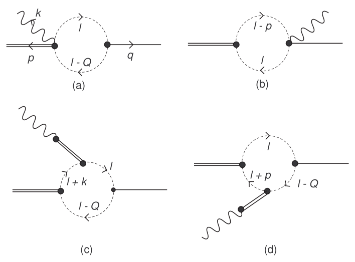
Figure 6: Feynman diagrams for the charged $K$ loop contributions to $\phi(p,\epsilon^{V})\rightarrow a_{0}(Q)+\gamma(k,\epsilon)$. The solid line denotes the $a_{0}$ meson, the wavy line the photon, the double solid line the vector mesons ($\rho$, $\omega$, $\phi$) and the dashed line the $K$ meson. $p$, $k$ and $Q$ are the momenta of the $\phi$ meson, the photon and the $a_{0}(980)$, respectively, and $l$ is the loop momentum.

The diagrams (c) and (d) each give the same result while (a) and (b) are required by gauge invariance. Notice from Eq. (2.3) that the direct photon-two pseudoscalar vertex vanishes in this model when $k=2$ is adopted, as we are doing here.  Thus the two pseudoscalars first couple to $\rho,\omega$ and $\phi$ which then transform to a photon as shown in Figs. (c) and (d). The strong vector-two pseudoscalar interaction vertices may be read from the fourth term of Eq. (2.2) while the scalar-two pseudoscalar interaction vertices are derived from the A, B, C and D terms of this equation (and explicitly given in Eq. (2.9)).

Note again that the Lagrangian density of Eq. (2.2) treats all of the pseudoscalars, scalars and vectors in a consistent chiral invariant manner. It can be modified to include gauge invariant photon interactions by making the replacements:

$$v_{\mu}\rightarrow{\tilde{v}}_{\mu} = v_{\mu}+\frac{1}{2}e{\cal A}_{\mu}\left(\xi Q\xi^{\dagger}+\xi^{\dagger}Q\xi\right),$$

$$p_{\mu}\rightarrow{\tilde{p}}_{\mu} = p_{\mu}+\frac{1}{2}e{\cal A}_{\mu}\left(\xi Q\xi^{\dagger}-\xi^{\dagger}Q\xi\right),$$

$$\rho_{\mu}\rightarrow{\tilde{\rho}}_{\mu} = \rho_{\mu}\ ,$$ (3.23)

where ${\cal A}$ and $Q$ were defined after Eq. (2.3). Under an infinitesimal electromagnetic gauge transformation with $\delta{\cal A}_{\mu}={\partial}_{\mu}\lambda(x)$, ${\tilde{p}}_{\mu}$ and ${\tilde{v}}_{\mu}-{\tilde{g}}{\tilde{\rho}}_{\mu}$ in Eq. (3.23) do not contain any terms proportional to ${\partial}_{\mu}\lambda(x)$. When substituted into Eq. (2.2), the above replacements yield, in addition to Eq. (2.3) the four field photon interaction terms in the Lagrangian density:

$$\frac{em_{v}^{2}}{{\tilde{g}}F_{\pi}^{2}}{\cal A}_{\mu}{\phi_{\mu}}K^{+}K^{-}+i\frac{e\gamma_{aKK}}{\sqrt{2}}{\cal A}_{\mu}a_{0}^{0}(K^{+}\partial_{\mu}K^{-}-K^{-}\partial_{\mu}K^{+})+\cdots\ ,$$ (3.24)

where $\phi_{\mu}$ is the $\phi$-meson field and $a_{0}^{0}$ is the neutral $a_{0}(980)$ scalar meson field.  Now it is straightforward to obtain the $K$ loop amplitudes (with the assumption $k=2$) for $\phi(p,\epsilon^{V})\rightarrow a_{0}(Q)+\gamma(k,\epsilon)$:

$$S_{a} = h\int\frac{d^{4}l}{i(2\pi)^{4}}\frac{[l\cdot(Q-l)][\epsilon\cdot\epsilon^{V}]}{[l^{2}+m_{K}^{2}][(Q-l)^{2}+m_{K}^{2}]},$$

$$S_{b} = -\frac{h}{2}\int\frac{d^{4}l}{i(2\pi)^{4}}\frac{[(2l-p)\cdot\epsilon^{V}][(2l-p)\cdot\epsilon]}{[l^{2}+m_{K}^{2}][(p-l)^{2}+m_{K}^{2}]},$$

$$S_{c}=S_{d} = -\frac{h}{2}\int\frac{d^{4}l}{i(2\pi)^{4}}\frac{[l\cdot(Q-l)][(2l+k)\cdot\epsilon][(2l+k-Q)\cdot\epsilon^{V}]}{[l^{2}+m_{K}^{2}][(Q-l)^{2}+m_{K}^{2}][(k+l)^{2}+m_{K}^{2}]},$$ (3.25)

where

$$h=\frac{em_{v}^{2}\gamma_{aKK}}{\sqrt{2}{\tilde{g}}F_{\pi}^{2}}\approx{\sqrt{2}}e{\tilde{g}}\gamma_{aKK},$$ (3.26)

and the KSRF relation was used in the last step. Note that the quantity defined in Eq. (2.8), $q^{2}=-Q^{2}$. To get the amplitude for the decay $\phi\rightarrow f_{0}\gamma$ we should replace $\gamma_{aKK}$ by $\gamma_{fKK}$ in Eq. (3.26).

The next step is to regulate the divergences which occur in these amplitudes. We employ the dimensional regularization scheme and thus continue from 4 to $d$ space-time dimensions according to the formula:

$$\int\frac{d^{d}l}{i(2\pi)^{d}}\frac{1}{(l^{2}+s)^{n}}=\frac{\Gamma(n-d/2)}{(4\pi)^{d/2}\Gamma(n)s^{n-d/2}},$$ (3.27)

where $n$ is an integer while $s$ is arbitrary. The physical amplitudes will emerge in the limit when $\epsilon=4-d\rightarrow 0$. It is convenient to define:

$$\frac{1}{{\bar{\epsilon}}}=\frac{2}{\epsilon}-\gamma+\ln(4\pi),$$ (3.28)

where $\gamma\approx$ 0.577 is the Euler-Mascheroni constant.

For $S_{a}$ we use the identity $l\cdot Q-l^{2}=-1/2[(l-Q)^{2}+m_{K}^{2}]-1/2(l^{2}+m_{K}^{2})+(m_{K}^{2}+Q^{2}/2)$ to write:

$$S_{a}=ih\delta_{\mu\nu}\epsilon^{V}_{\mu}(p)\epsilon_{\nu}(k)[-A_{0}(m_{K}^{2})+\frac{1}{2}(2m_{K}^{2}+Q^{2})B_{0}(Q^{2})],$$ (3.29)

where

$$A_{0}(m_{K}^{2}) = \int\frac{d^{d}l}{i(2\pi)^{d}}\frac{1}{l^{2}+m_{K}^{2}}\ ,$$

$$B_{0}(Q^{2}) = \int\frac{d^{d}l}{i(2\pi)^{d}}\frac{1}{[l^{2}+m_{K}^{2}][(l-Q)^{2}+m_{K}^{2}]}\ .$$ (3.30)

For $S_{b}$ we define:

$$S_{b} = -i\frac{h}{2}\epsilon^{V}_{\mu}(p)\epsilon_{\nu}(k)B_{\mu\nu}(p),$$

$$B_{\mu\nu}(p) = \int\frac{d^{d}l}{i(2\pi)^{d}}\frac{(2l-p)_{\mu}(2l-p)_{\nu}}{[l^{2}+m_{K}^{2}][(p-l)^{2}+m_{K}^{2}]}\ .$$ (3.31)

Finally, for the triangle diagrams we similarly rearrange the numerator to get:

$$S_{c}=S_{d} = -i\frac{h}{2}\epsilon^{V}_{\mu}(p)\epsilon_{\nu}(k)[-\frac{1}{2}B_{\mu\nu}(k)+{Q_{\mu}}{B_{\nu}}(-k)+\frac{1}{2}{Q_{\mu}}{k_{\nu}}{B_{0}}(k^{2})$$ (3.32)

$$- \frac{1}{2}B_{\mu\nu}(p)-{B_{\mu}}(p)Q_{\nu}+\frac{1}{2}{p_{\mu}}{Q_{\nu}}{B_{0}}(p^{2})+\frac{1}{2}(2m_{K}^{2}+Q^{2})X_{\mu\nu}(p,k)],$$

wherein $B_{0}(p^{2})$ and $B_{\mu\nu}(p)$ have been already defined while,

$$B_{\mu}(p)=\int\frac{d^{d}l}{i(2\pi)^{d}}\frac{l_{\mu}}{[l^{2}+m_{K}^{2}][(l-p)^{2}+m_{K}^{2}]},$$ (3.33)

and

$$X_{\mu\nu}(p,k)=\int\frac{d^{d}l}{i(2\pi)^{d}}\frac{(2l+k-Q)_{\mu}(2l+k)_{\nu}}{[l^{2}+m_{K}^{2}][(Q-l)^{2}+m_{K}^{2}][(k+l)^{2}+m_{K}^{2}]}.$$ (3.34)

Note that $k^{2}=0$ since it corresponds to a physical photon momentum.

Using Feynman’s trick for combining denominators and Eqs. (3.27) and (3.28) we evaluate the integral $B_{0}(p^{2})$ near $d=4$:

$$B_{0}(p^{2}) = \frac{1}{(4\pi)^{2}}[\frac{1}{{\bar{\epsilon}}}-F_{0}(p^{2})],$$

$$F_{0}(p^{2}) = \int^{1}_{0}dx\ln[m_{K}^{2}-x(x-1)p^{2}].$$ (3.35)

We also find

$$B_{\mu}(p)=\frac{1}{2}p_{\mu}B_{0}(p^{2}).$$ (3.36)

The presence of a pole at $d=4$ indicated by the term $1/{\bar{\epsilon}}$ corresponds, of course, to a logarthmic divergence in the cutoff regularization method.

Using the integrals defined above we can compactly write the total amplitude as:

$$S = S_{a}+S_{b}+S_{c}+S_{d}$$ (3.37)

$$= i\frac{h}{2}\epsilon^{V}_{\mu}(p)\epsilon_{\nu}(k)[\delta_{\mu\nu}(-2A_{0}(m_{K}^{2})+(2m_{K}^{2}+Q^{2})B_{0}(q^{2}))+B_{\mu\nu}(k)$$

$$- (2m_{K}^{2}+Q^{2})X_{\mu\nu}(p,k)].$$

Notice, in particular, that the contribution of $S_{b}$ has cancelled out against a piece of the triangle diagrams.

The evaluation of an integral of the form $B_{\mu\nu}(p)$ is a little more complicated. We use covariance (in $d$-dimensions) to relate it to the other integrals as:

$$B_{\mu\nu}(p) = \delta_{\mu\nu}\frac{4}{1-d}[-\frac{A_{0}(m_{K}^{2})}{2}+(m_{K}^{2}+\frac{p^{2}}{4})B_{0}(p^{2})]$$ (3.38)

$$+ {p_{\mu}}p_{\nu}[\frac{4}{p^{2}}((1+\frac{1}{2}\frac{d}{1-d})A_{0}(m_{K}^{2})-m_{K}^{2}(1+\frac{d}{1-d})B_{0}(p^{2})$$

$$- \frac{p^{2}}{4}\frac{d}{1-d}B_{0}(p^{2}))-B_{0}(p^{2})].$$

We see that $B_{\mu\nu}$ contains the integral $A_{0}(m_{K}^{2})$ which is noted from Eq. (3.30) to involve a quadratic divergence in the cut-off regularization scheme. In the dimensional regularization approach this corresponds  [35] to a pole at $d=2$, as may be seen from Eq. (3.27). It is necessary to check that this divergence cancels out in the total amplitude. This may be done by using Eq. (3.38) to get, near $d=2$:

$$B_{\mu\nu}(k)|_{k^{2}=0}=2A_{0}(m_{K}^{2})\delta_{\mu\nu}+\cdots\ ,$$ (3.39)

where the three dots indicate terms not containing $A_{0}(m_{K}^{2})$. Substituting this into Eq. (3.37) (considered at d=2) shows that all dependence on $A_{0}(m_{K}^{2})$ at $d=2$ is cancelled, as desired. We interpret this as the cancellation of the quadratic divergences in the individual diagrams.

For the physical case we must consider, of course, the amplitude evaluated near $d=4$. The integral $A_{0}(m_{K}^{2})$ is, near $d=4$:

$$A_{0}(m_{K}^{2})=-\frac{m_{K}^{2}}{(4\pi)^{2}}\left[\frac{1}{{\bar{\epsilon}}}+1-\ln(m_{K}^{2})\right]\ .$$ (3.40)

Using Eq. (3.38) we find for $B_{\mu\nu}(k)$ near $d=4$ and $k^{2}=0$:

$$B_{\mu\nu}(k)=2A_{0}(m_{K}^{2})\delta_{\mu\nu}+\frac{1}{3(4\pi)^{2}}k_{\mu}k_{\nu}\left[\frac{1}{{\bar{\epsilon}}}-\ln(m_{K}^{2})+\frac{2}{3}\right]\ ,$$ (3.41)

wherein the first term was separated for convenience. Note that the ${k_{\mu}}k_{\nu}$ term will not contribute to the physical amplitude because it gets multiplied by the photon polarization vector $\epsilon_{\nu}(k)$. Now substituting Eq. (3.41) into the total amplitude, Eq. (3.37), shows that its effect is simply to cancel the $-2A_{0}(m_{K}^{2})$ term.

To evaluate the remaining, $X_{\mu\nu}(p,k)$ term we first use covariance to express it as:

$$X_{\mu\nu}(p,k)=\delta_{\mu\nu}X_{1}+p_{\mu}p_{\nu}X_{2}+k_{\mu}k_{\nu}X_{3}+p_{\mu}k_{\nu}X_{4}+k_{\mu}p_{\nu}X_{5}\ ,$$ (3.42)

where each of the $X_{i}$ depends on $p^{2}$ and $p{\cdot}k$. The $X_{i}$ may be determined by calculating $X_{\mu\mu}$, $k_{\mu}X_{\mu\nu}$, $p_{\nu}X_{\mu\nu}$ and $k_{\mu}p_{\nu}X_{\mu\nu}$ both from Eq. (3.42) and from Eq. (3.34). This leads to the relations (remembering $k^{2}=0$):

$$X_{2} = 0,$$

$$B_{0}(Q^{2}) = X_{1}+k{\cdot}pX_{5},$$

$$0 = k{\cdot}pX_{3}+p^{2}X_{4},$$

$$X_{5} = \frac{1}{(p{\cdot}k)^{2}}[\frac{p^{2}}{d-2}(B_{0}(Q^{2})-B_{0}(p^{2}))+(p{\cdot}k+\frac{Q^{2}-p^{2}}{d-2})B_{0}(Q^{2})$$ (3.43)

$$+ \frac{4m_{K}^{2}k{\cdot}p}{d-2}C(p^{2},k{\cdot}p)],$$

where the finite integral $C(p^{2},k{\cdot}p)$ is given by:

$$C(p^{2},k{\cdot}p)=\int\frac{d^{4}l}{i(2\pi)^{4}}\frac{1}{[l^{2}+m_{K}^{2}][(l-Q)^{2}+m_{K}^{2}][(l+k)^{2}+m_{K}^{2}]}.$$ (3.44)

Actually, only the coefficients $X_{1}$ and $X_{5}$ remain after $X_{\mu\nu}$ is multiplied by the polarization vectors of the photon and $\phi$ meson; furthermore these two coefficients are related as above. Substituting back into the total amplitude, Eq. (3.37) and making use of the cancellation between the $A_{0}(m_{K}^{2})$ and $B_{\mu\nu}(k)$ terms discussed before, yields:

$$S = i\,\frac{h}{2}\,\epsilon^{V}_{\mu}(p)\epsilon_{\nu}(k)\left(-\frac{\delta_{\mu\nu}}{p{\cdot}k}+\frac{k_{\mu}p_{\nu}}{(p{\cdot}k)^{2}}\right)(2m_{K}^{2}+Q^{2})\Biggl{[}\frac{p^{2}}{2}\left\{B_{0}(Q^{2})-B_{0}(p^{2})\right\}$$ (3.45)

$${}+2m_{K}^{2}(p{\cdot}k)C(p^{2},p{\cdot}k)-\frac{p{\cdot}k}{(4\pi)^{2}}\Biggr{]}\ .$$

Note that the last term arises from the $1/\epsilon$ term in $B_{0}(Q^{2})$ multiplying the leading $\epsilon$ term of its factor. From Eq. (3.35) we see that the logarithmic divergences cancel out of the difference $(B_{0}(Q^{2})-B_{0}(p^{2}))$. Thus the final amplitude is completely finite; both the logarithmic and quadratic divergences have been seen to cancel using regularized expressions for everything. The quadratic divergences arose in the first place because of the derivative-type interactions required by use of the non linear sigma model terms to describe the pseudoscalar meson interactions. In addition, the starting Lagrangian treated the vector and scalar mesons in the same chiral invariant framework.

Evaluation of the finite integrals in Eq. (3.45) yields the final expression for the Feynman amplitude, $iS$:

$$iS = -\frac{h}{2}\frac{1}{(4\pi)^{2}}\epsilon^{V}_{\mu}(p)\epsilon_{\nu}(k)(-\frac{\delta_{\mu\nu}}{p\cdot k}+\frac{k_{\mu}p_{\nu}}{(p{\cdot}k)^{2}})(2m_{K}^{2}+Q^{2})\biggl{\{}-p{\cdot}k$$ (3.46)

$$+ \frac{p^{2}}{2}\left(\sigma(p^{2})[\ln\frac{1+\sigma(p^{2})}{1-\sigma(p^{2})}-i\pi]-\sigma(Q^{2})[\ln\frac{1+\sigma(Q^{2})}{1-\sigma(Q^{2})}-i\pi]\right)$$

$$+ \frac{m_{K}^{2}}{2}\left([\ln\frac{1+\sigma(p^{2})}{1-\sigma(p^{2})}-i\pi]^{2}-[\ln\frac{1+\sigma(Q^{2})}{1-\sigma(Q^{2})}-i\pi]^{2}\right)\biggr{\}},$$

where,

$$\sigma(p^{2}) = \sqrt{1+\frac{4m_{K}^{2}}{p^{2}}},$$

$$\sigma(Q^{2}) = \sqrt{1+\frac{4m_{K}^{2}}{Q^{2}}},$$ (3.47)

Note that Eq. (3.46) holds only in the kinematical range where $-Q^{2}=q^{2}>4m_{K}^{2}$; the positive quantity, $q$ was also defined in Eq. (2.8). Furthermore note that $p^{2}=-m_{\phi}^{2}$. In the kinematical range where $-Q^{2}=q^{2}<4m_{K}^{2}$, one should replace

$$[\ln\frac{1+\sigma(Q^{2})}{1-\sigma(Q^{2})}-i\pi] \rightarrow -2i\tan^{-1}\frac{1}{{\tilde{\sigma}}(Q^{2})},$$

$$\sigma(Q^{2})\rightarrow i{\tilde{\sigma}}(Q^{2}) = i\sqrt{-1-\frac{4m_{K}^{2}}{Q^{2}}}\ ,$$ (3.48)

in Eq. (3.46) above.

4 Comparing the $K$ loop with experiment

The expression in Eq. (3.46) describes the decay $\phi\rightarrow a_{0}\gamma$. To get the Feynman amplitude for $\phi\rightarrow\pi^{0}\eta\gamma$, we should multiply Eq. (3.46) by the factor $(q_{1}\cdot q_{2})D_{a_{0}}(q^{2})\gamma_{a_{0}\pi\eta}$, where $D_{a_{0}}(q^{2})$ was defined in Eq. (2.7). This assumes a simple form for the $a_{0}$ propagator, which can only be an approximation. However our main concern here is an initial exploration of the resonance region in the present framework so it seems reasonable for now. We write the resulting Feynman amplitude as

$$iS(\phi\rightarrow\pi^{0}\eta\gamma)=e(q_{1}\cdot q_{2})X^{(\pi\eta)}_{a_{0}}\left[(p\cdot k)(\epsilon^{V}\cdot\epsilon)-(p\cdot\epsilon)(k\cdot\epsilon^{V})\right]\ ,$$ (4.49)

which thereby defines $X^{(\pi\eta)}_{a_{0}}$. Note that the sum $X^{(\pi\eta)}_{a_{0}}+Y^{(\pi\eta)}_{a_{0}}$, where $Y^{(\pi\eta)}_{a_{0}}$ is defined in Eq. (2.6), would correspond to a model containing both the $K$ loop contribution to the resonant amplitude as well as a point vertex contribution to the resonant amplitude. For now we focus on the $K$-loop contribution. The decay spectrum shape, $d\Gamma/dq$ is then obtained by replacing $Y^{(\pi\eta)}_{a_{0}}$ in Eq. (2.10) by $X^{(\pi\eta)}_{a_{0}}$. Conventionally, one uses instead,

$$\frac{dB(\phi\rightarrow\pi^{0}\eta\gamma)}{dq}=\frac{1}{\Gamma(\phi)}\frac{d\Gamma(\phi\rightarrow\pi^{0}\eta\gamma)}{dq}\ ,$$ (4.50)

where $\Gamma(\phi)=4.26$ MeV.

In section 2.1 we observed that, even though the use of derivative type SPP coupling helped somewhat, the tree interaction involving the $a_{0}(980)$ resonance was unable to explain the shape of the peak at large $q$ in the experimental data for $dB(\phi\rightarrow\pi^{0}\eta\gamma)/dq$. Now we will look at the result of using the $K$-loop amplitude for this purpose. Taking [26] $m_{a}=985$ MeV and $\Gamma_{a}=50$-$100$ MeV, the only quantity which is not well known is the product of the scalar meson coupling constants $\gamma_{aKK}\gamma_{a\pi\eta}$. In Fig. 7, it is shown that a choice $\gamma_{aKK}\gamma_{a\pi\eta}=125\,\mbox{GeV}^{-2}$ can nicely explain the shape of the experimental data in the region of $q$ near the $a_{0}(980)$ resonance.

Figure 7: Predicted $dB(\phi\rightarrow\pi^{0}\eta\gamma)/dq$ in the region of the $a_{0}(980)$ resonance with $\gamma_{aKK}\gamma_{a\pi\eta}=125\,\mbox{GeV}^{-2}$ and $\Gamma_{a}=0.1$ GeV. The vertical scale has units $10^{-7}\,\mbox{MeV}^{-1}$. Experimental data are as in Fig. 2.

For $q$ below the resonance region, the $K$ loop contribution in the present model falls off rapidly, as one might reasonably expect with derivative coupling, and lies lower than the data points. In addition to the nonresonant background [9] which is usually included to explain this region, there might be some tree level resonance production which was observed in Fig. 2 to peak around $950$ MeV.

The main feature of the data is that there is a very rapid falloff with apparent discontinuity of the slope, when $q$ reaches the $K{\bar{K}}$ threshold. This is a clear signal for the importance of the $K$ loop contribution. One may see this feature by referring to Fig. 8, for which the $a_{0}(980)$ mass has been artificially lowered to $970$ MeV. Comparing with the previous figure shows that the sharp fall-off is exactly the same in both cases, clearly unaffected by the difference of assumed resonance masses in the two cases. The difference in masses, on the other hand, shows up as a difference in position of the peaks. It should be remarked that the peak position is also affected by the decreasing phase space with increasing $q$. This characteristic feature of the $K$-loop contribution was first illustrated by Achasov [36] by considering the behavior of the result with lowered values of the $K$-meson mass.

Figure 8: Predicted $dB(\phi\rightarrow\pi^{0}\eta\gamma)/dq$ in the region of the $a_{0}(980)$ resonance but where the $a_{0}$ mass was artificially lowered to $970$ MeV. Here $\gamma_{aKK}\gamma_{a\pi\eta}=115\,\mbox{GeV}^{-2}$ and $\Gamma_{a}=0.1$ GeV. Experimental data are as in Fig. 2.

Next, let us check the dependence of the prediction on the width of $a_{0}(980)$. Figure 9 shows that the predicted $dB(\phi\rightarrow\pi^{0}\eta\gamma)/dq$ in the region of the $a_{0}$(980) resonance with $\gamma_{aKK}\gamma_{a\pi\eta}=95\mbox{GeV}^{-2}$ and $\Gamma_{a}=0.05$ GeV.

Figure 9: Predicted $dB(\phi\rightarrow\pi^{0}\eta\gamma)/dq$ in the region of the $a_{0}(980)$ resonance with $\gamma_{aKK}\gamma_{a\pi\eta}=95\,\mbox{GeV}^{-2}$ and $\Gamma_{a}=0.05$ GeV. Experimental data are as in Fig. 2.

Comparing this prediction with that given in Fig. 7, we see that the smaller $a_{0}$ width gives a sharper peak, and that a smaller value of $\gamma_{aKK}\gamma_{a\pi\eta}$ can also reproduce the experimental data at the peak position. For further decreasing the value of $\gamma_{aKK}\gamma_{a\pi\eta}$ the inclusion of the $K$-loop correction into the propagator of $a_{0}(980)$ may be important as pointed out in Ref. [36].

The $K$-loop contribution to the branching distribution, $dB(\phi\rightarrow\pi^{0}\pi^{0}\gamma)/dq$ may be similarly evaluated and compared to experiment. There is similarly a problem for the tree level resonance model to reproduce this experimental shape in the high $q$ region. The $K$ loop amplitude $\phi\rightarrow f_{0}(980)\gamma$ is given by Eq. (3.46) wherein the overall factor $h$ is now obtained by replacing $\gamma_{aKK}$ in Eq. (3.26) by $\gamma_{fKK}$. To get the Feynman amplitude for $\phi\rightarrow\pi^{0}\pi^{0}\gamma$, we should multiply Eq. (3.46) by the factor $\sqrt{2}(q_{1}\cdot q_{2})D_{f_{0}}(q^{2})\gamma_{f_{0}\pi\pi}$, where $D_{f_{0}}(q^{2})$ was defined in Eq. (2.19). This defines $X^{(\pi\pi)}_{f_{0}}$ as in Eq. (4.49). The spectrum shape is determined by using Eq. (2.17) with $X^{(\pi\pi)}_{f_{0}}$ replacing $Y^{(\pi\pi)}_{f_{0}}$ .

Taking [26] $m_{f}=980\pm 10$ MeV and $\Gamma_{f}=40$-$100$ MeV, the only quantity which is not well known is the product of the scalar meson coupling constants $\gamma_{fKK}\gamma_{f\pi\pi}$. In Fig. 10, it is shown that a choice $\gamma_{aKK}\gamma_{f\pi\pi}=86\,\mbox{GeV}^{-2}$ can nicely explain the shape of the experimental data in the region of $q$ near the $f_{0}(980)$ resonance.

Figure 10: Predicted $dB(\phi\rightarrow\pi^{0}\pi^{0}\gamma)/dq$ in the region of the $f_{0}(980)$ resonance with $\gamma_{fKK}\gamma_{f\pi\pi}=86\,\mbox{GeV}^{-2}$ and $\Gamma_{f}=0.1$ GeV. The vertical scale has units $10^{-8}\mbox{MeV}^{-1}$.

As in the case of the $\phi\rightarrow\pi^{0}\eta\gamma$ process, the $K$-loop description of $dB/dq$ only explains the upper $q$ region near the scalar resonance. To cover the lower $q$ region some non resonant background [9] is required. Possibly a tree level resonant background, corresponding to using $X^{(\pi\pi)}_{f_{0}}+Y^{(\pi\pi)}_{f_{0}}$ in Eq. (2.17), would also be appropriate.

In both cases considered in this section, it is also desirable to include the effects of using multichannel scalar meson propagators [37] for a better approximation to the detailed dynamics. A very recent treatment of the $\phi\rightarrow\pi^{0}\pi^{0}\gamma$ process in this framework is given in [38].

5 Summary and discussion

Historically, the study of elementary particle spectroscopy has been built around the organization of these particles into SU(3) flavor multiplets and the consequent predicted (broken symmetry) mass formulas and interaction vertices. The still mysterious scalars can be expected to yield up some of their secrets by this type of analysis. Indeed some recent analyses have already been carried out [17, 39, 40, 41, 42]. The most dramatic feature is that the light scalars appear to exhibit, as originally suggested by Jaffe [43], a reverse mass ordering compared to the other meson multiplets.

In Ref. [12] an attempt was made to extend the SU(3) analysis to relate all the decays of the types S$\rightarrow\gamma\gamma$, V$\rightarrow$S$\gamma$ and S$\rightarrow$V$\gamma$ to each other by using a simple effective VVS point-like interaction, together with vector meson dominance. The analogous assumption [13] of a point-like VVP structure was very successful [44] in phenomenologically correlating P$\rightarrow\gamma\gamma$, V$\rightarrow$P$\gamma$ and P$\rightarrow$V$\gamma$ decays. Such an approach was the original motivation which led to the present investigation. In section 2 we compared the spectrum shape of the decays $\phi\rightarrow\eta\pi^{0}$, measuring the effects of an intermediate $a_{0}(980)$ resonance and $\phi\rightarrow\pi^{0}\pi^{0}$, measuring the effects of an intermediate $f_{0}(980)$ resonance, in the point like VVS model with the corresponding experimental observations. It was found that the resonant peaks in the model were pushed lower due to decreasing phase space. This contrasted with experiment which does not indicate this effect. On the other hand, if one were to use a tree model of this type with non derivative SPP type couplings, the resonant peaks were seen to get completely washed out. This would appear to be an advantage for the derivative coupling, which is dictated by chiral symmetry in the present framework. Nevertheless, since even with derivative coupling the spectrum shape is not very well fitted, there must be another mechanism at work.

Now, it has been emphasized [36] that the $K$-loop model for the $\phi$ radiative decays constitutes a special mechanism which does give a characteristic spectrum shape in agreement with experiment. This is readily understandable since the $\phi(1020)$ meson is just a little bit heavier than the two $K$ mesons which comprise its main decay product. We thus studied the $K$-loop diagrams using the chiral Lagrangian of pseudoscalars, vectors and scalars given in Eqs. (2.2) and (2.4) with the relevant photon terms introduced by the substitutions shown in Eq. (3.23). Most of the calculations of this process have not started from a chiral symmetric Lagrangian and have thus used non-derivative type SPP type interaction vertices. The use of derivative coupling introduces an extra complication in that there is an new diagram, shown as (b) in Fig. 6. In addition, individual diagrams now contain quadratic as well as logarithmic divergences. It is known that these divergences are forced to cancel from gauge invariance. However we have used the dimensional regularization scheme and shown explicitly in section 3 that both the log and quadratic divergences cancel in the regularized expressions. This may be of some interest in dealing with processes of the present type.

In section 4, we observed that the shape of the $a_{0}(980)$ and $f_{0}(980)$ resonance regions in the $\phi$ radiative decays could be explained by the corresponding $K$-loop amplitudes. Furthermore, it was evident that the characteristic sharp drop in the amplitude at large $q^{2}$ was associated with the the $K{\bar{K}}$ threshold rather than with the falloff of the resonance away from its peak. For this work, we used the coupling constant products $\gamma_{aKK}\gamma_{a\pi\eta}$ and $\gamma_{fKK}\gamma_{f\pi\pi}$ respectively as fitting parameters for the $\phi$ radiative decay spectra into $\pi^{0}\eta$ and $\pi^{0}\pi^{0}$. Elsewhere, we plan to study more precisely the values of these coupling constants obtained by comparing with experiment, chiral models of meson meson scattering in which the same interactions are used. We also will study how the point-like diagrams with resonant contributions discussed in section 2 can be used in conjunction with the $K$-loop diagrams to improve the fit to the resonant region. This will presumably become even more interesting when more data points become available. Another point of interest concerns the extent to which the various SPP coupling constants can be correlated assuming a single nonet of scalars. This arises because there is some evidence [45] that two scalar nonets (one presumably made from 4 quarks and the other from two quarks) mix to make up the physical scalar states. A recent exploration of the effect of such a mixture on $\phi(1020)$ radiative decays has been given in Ref. [46]. Still another correction to the simple picture employed here would be to use more realistic resonance propagators by including pseudoscalar loops [37].

Of course, in order to make a careful comparison with experiment one should include non-resonant contributions which are expected to dominate for small $q$. These will include the emission of a pion with a virtual $\rho$ which subsequently decays into $\pi\gamma$ (and similar diagrams leading to a $\pi^{0}\eta\gamma$ final state) as discussed in Ref. [9]. There will also be non resonant contributions from the $K$-loop diagrams. A variety of interference mechanisms to explain the full spectrum are discussed in Ref. [47]. It should be noted that the “background” contributions may very well have a non-trivial effect also in the resonance region itself.

Using the results obtained here and taking into account the features just discussed, we will continue to study the $\phi$ radiative decays with the expectation that it may contribute to the understanding of the puzzling scalar mesons and ultimately to low energy QCD.

DEDICATION: We are pleased to dedicate this paper to Rafael Sorkin in connection with the world wide web celebration of his sixtieth birthday. We have benefited a great deal from our interactions with Rafael. We wish him good health and continued success in his endeavor to understand the deepest mysteries of space-time structure.

References

- [1]
- [2] [] e-mail: dblack@jlab.org
- [3]
- [4] [] e-mail: harada@phys.nagoya-u.ac.jp
- [5]
- [6] [] e-mail: schechte@physics.syr.edu
- [7] M. N. Achasov et al. [SND Collaboration], Phys. Lett. B 479, 53 (2000); R. R. Akhmetshin et al. [CMD-2 Collaboration], Phys. Lett. B 462, 380 (1999); A. Aloisio et al. [KLOE Collaboration], arXiv:hep-ex/0107024; Phys. Lett. B 537, 21 (2002); Phys. Lett. B 536, 209 (2002).
- [8] See the proceedings of the conferences: S. Ishida et al “Possible existence of the sigma meson and its implication to hadron physics”, KEK Proceedings 2000-4, Soryyushiron Kenkyu 102, No. 5, 2001; D. Amelin and A. M. Zaitsev, “Hadron spectroscopy: ninth international conference on hadron spectroscopy HADRON 2001, AIP conference proceedings No. 619; A. H. Fariborz, “Scalar mesons: an interesting puzzle for QCD”, SUNY Institute of Technology, Utica, NY, 16-18 May 2003, AIP conference proceedings No. 688.
- [9] N. N. Achasov and V. N. Ivanchenko, Nucl. Phys. B 315, 465 (1989).
- [10] F. E. Close, N. Isgur and S. Kumano, Nucl. Phys. B 389, 513 (1993); N. N. Achasov and V. V. Gubin, Phys. Rev. D 56, 4084 (1997); Phys. Rev. D 57, 1987 (1998); N. N. Achasov, V. V. Gubin and V. I. Shevchenko, Phys. Rev. D 56, 203 (1997); J. L. Lucio Martinez and M. Napsuciale, Phys. Lett. B 454, 365 (1999); Phys. Lett. B 454, 365 (1999); arXiv:hep-ph/0001136; A. Bramon, R. Escribano, J. L. Lucio Martinez, M. Napsuciale and G. Pancheri, Phys. Lett. B 494, 221 (2000).
- [11] S. Weinberg, Phys. Rev. Lett. 17, 616 (1966).
- [12] D. Black, M. Harada and J. Schechter, Phys. Rev. Lett. 88, 181603 (2002) [arXiv:hep-ph/0202069]. See also arXiv:hep-ph/0306065 for some additional discussion.
- [13] M. Gell-Mann, D. Sharp and W. G. Wagner, Phys. Rev. Lett. 8, 261 (1962). A general formulation of the interaction in a gauge invariant manner was given in: T. Fujiwara, T. Kugo, H. Terao, S. Uehara and K. Yamawaki, Prog. Theor. Phys. 73, 926 (1985); O. Kaymakcalan, S. Rajeev and J. Schechter, Phys. Rev. D 30, 594 (1984); O. Kaymakcalan and J. Schechter, Phys. Rev. D 31, 1109 (1985); P. Jain, R. Johnson, U. G. Meissner, N. W. Park and J. Schechter, Phys. Rev. D 37, 3252 (1988).
- [14] F. E. Close, N. Isgur and S. Kumano, Nucl. Phys. B 389, 513 (1993) [arXiv:hep-ph/9301253]; J. E. Palomar, L. Roca, E. Oset and M. J. Vicente Vacas, Nucl. Phys. A 729, 743 (2003) [arXiv:hep-ph/0306249].
- [15] C. G. Callan, S. Coleman, J. Wess and B. Zumino, Phys. Rev. 177, 2247 (1969).
- [16] M. Harada and J. Schechter, Phys. Rev. D 54, 3394 (1996).
- [17] D. Black, A. H. Fariborz, F. Sannino and J. Schechter, Phys. Rev. D 59, 074026 (1999).
- [18] M. Bando, T. Kugo and K. Yamawaki, Phys. Rept. 164, 217 (1988).
- [19] M. Harada and K. Yamawaki, Phys. Rept. 381, 1 (2003) [arXiv:hep-ph/0302103].
- [20] O. Kaymakcalan, S. Rajeev and J. Schechter, Phys. Rev. D 30, 594 (1984); O. Kaymakcalan and J. Schechter, Phys. Rev. D 31, 1109 (1985);
- [21] J. Schechter, Phys. Rev. D 34, 868 (1986); K. Yamawaki, Phys. Rev. D 35, 412 (1987); M. F. Golterman and N. D. Hari Dass, Nucl. Phys. B 277, 739 (1986); U. G. Meissner and I. Zahed, Z. Phys. A 327, 5 (1987).
- [22] A. M. Abdel-Rehim, D. Black, A. H. Fariborz and J. Schechter, Phys. Rev. D 67, 054001 (2003) [arXiv:hep-ph/0210431].
- [23] J.J. Sakurai, Currents and mesons (Chicago U.P., Chicago, 1969). In the present context, see for example. J. Schechter, Phys. Rev. D 34, 868 (1986).
- [24] K. Kawarabayashi and M. Suzuki, Phys. Rev. Lett. 16, 255 (1966): Riazuddin and Fayyazuddin, Phys. Rev. 147, 1071 (1966).
- [25] In M. Harada and K. Yamawaki, Phys. Rev. Lett. 87, 152001 (2001), it was shown that this is also satisfied even at the quantum level in three flavor QCD.
- [26] S. Eidelman et al. [Particle Data Group], Phys. Lett. B 592, 1 (2004) and 2005 Partial update for edition 2006 (URL: http://pdg.lbl.gov).
- [27] A. H. Fariborz and J. Schechter, Phys. Rev. D 60, 034002 (1999) [arXiv:hep-ph/9902238].
- [28] D. Black, A. H. Fariborz and J. Schechter, Phys. Rev. D 61, 074030 (2000) [arXiv:hep-ph/9910351].
- [29] See the result of the SND Collaboration in [7] above.
- [30] N. N. Achasov and A. V. Kiselev, Phys. Rev. D 70, 111901 (2004) [arXiv:hep-ph/0405128].
- [31] See the result of the KLOE Collaboration in [7] above.
- [32] M. Harada, F. Sannino and J. Schechter, Phys. Rev. D 54, 1991 (1996) [arXiv:hep-ph/9511335].
- [33] M. N. Achasov et al., Phys. Lett. B 485, 349 (2000) [arXiv:hep-ex/0005017].
- [34] A. Aloisio et al. [KLOE Collaboration], Phys. Lett. B537, 21 (2002) [arXiv:hep-ex/0204013].
- [35] M. J. G. Veltman, Acta Phys. Polon. B 12, 437 (1981); see also Ref. [19].
- [36] N. N. Achasov, Nucl. Phys. A 728, 425 (2003).
- [37] N. N. Achasov, S. A. Devyanin and G. N. Shestakov, Sov. J. Nucl. Phys. 32(4), 566 (1980) and Z. Phys. C 22, 53 (1984); see also Ref. [30].
- [38] N. N. Achasov and A. V. Kisilev [arXiv:hep-ph/0512047].
- [39] V. Cirigliano, G. Ecker, H. Neufeld and A. Pich, JHEP 0306, 012 (2003) [arXiv:hep-ph/0305311].
- [40] J. A. Oller, Nucl. Phys. A 727, 353 (2003) [arXiv:hep-ph/0306031].
- [41] J. R. Pelaez, Mod. Phys. Lett. A 19, 2879 (2004) [arXiv:hep-ph/0411107].
- [42] L. Maiani, F. Piccinini, A. D. Polosa and V. Riquer, Phys. Rev. Lett. 93, 212002 (2004) [arXiv:hep-ph/0407017].
- [43] R. L. Jaffe, Phys. Rev. D 15, 267 (1977).
- [44] For a review see P. J. O’Donnell, Rev. Mod. Phys. 53, 673 (1981).
- [45] D. Black, A. H. Fariborz and J. Schechter, Phys. Rev. D 61, 074001 (2000) [arXiv:hep-ph/9907516]; D. Black, A. H. Fariborz, S. Moussa, S. Nasri and J. Schechter, Phys. Rev. D 64, 014031 (2001) [arXiv:hep-ph/0012278]; T. Teshima, I. Kitamura and N. Morisita, J. Phys. G 28, 1391 (2002) [arXiv:hep-ph/0105107]; J. Phys. G 30, 663 (2004) [arXiv:hep-ph/0305296]; Nucl. Phys. A 759, 131 (2005) [arXiv:hep-ph/0501073]; F. E. Close and N. A. Tornqvist, J. Phys. G 28, R249 (2002) [arXiv:hep-ph/0204205]; A. H. Fariborz, Int. J. Mod. Phys. A 19, 2095 (2004) [arXiv:hep-ph/0302133]; M. Napsuciale and S. Rodriguez, Phys. Rev. D 70, 094043 (2004) [arXiv:hep-ph/0407037]; A. H. Fariborz, R. Jora and J. Schechter, Phys. Rev. D 72, 034001 (2005)[arXiv:hep-ph/0506170]
- [46] T. Teshima, I. Kitamura and N. Morisita, J. Phys. G 28, 1391 (2002) [arXiv:hep-ph/0105107].
- [47] A. Gokalp, A. Kuckarslan, S. Solmaz and O. Yilmaz, J. Phys. G 28, 2783 (2002) [Erratum-ibid. G28, 3021 (2002)] [arXiv:hep-ph/0205016].