Coupling of $\bar{K}^{*}N$ to the $\Lambda(1520)$

Abstract

We study the coupling of the $\Lambda(1520)\equiv\Lambda^{*}$ resonance to the $\bar{K}^{*}$ vector meson and nucleon. This coupling is not directly measured from the resonance decay, but is expected to be important in hyperon production reactions, in particular for the exotic $\Theta^{+}$ production. We compute the coupling in two different schemes, one in the chiral unitary model where the $\Lambda^{*}$ is dominated by the quasibound state of mesons and baryons, and the other in the quark model where the resonance is a $p$-wave excitation in the three valence quarks. Although it is possible to construct both models such that they reproduce the $\bar{K}N$ and $\pi\Sigma$ decays, there is a significant difference between the $\Lambda^{*}\bar{K}^{*}N$ couplings in the two models. In the chiral unitary model $|g_{\Lambda^{*}\bar{K}^{*}N}|\sim 1.5$, while in the quark model $|g_{\Lambda^{*}\bar{K}^{*}N}|\sim 10$. The difference of the results stems from the different structure of the $\Lambda^{*}$ in both models, and hence, an experimental determination of this coupling would shed light on the nature of the resonance.

I Introduction

Recent activities in hadron physics have been much stimulated by the discussions on exotic states. The existence of the exotic pentaquark $\Theta^{+}$ Nakano:2003qx is not yet confirmed, but much of the works are related to explain its expectedly unusual properties.

Exotic states, by definition, contain more than three quarks in the case of baryons, and more than one quark-antiquark pair in the case of mesons. In both cases, the exotic states may have components of two or more color singlet states. If the color-singlet correlations such as $[\bar{q}q]_{\text{singlet}}$ and $[qqq]_{\text{singlet}}$ are strong, the states may be regarded as composite states of two or more hadrons. However, if the color-nonsinglet correlations such as diquark correlations are strong, the components of color singlet states are only a small part of the exotic states.

Such color-singlet or color-nonsinglet correlations may be tested not only in the manifestly exotic states but also in ordinary hadrons. The role of diquark correlations in hadrons has been discussed Jaffe:2004ph ; Jaffe:2005md . Contrary, the importance of color-singlet correlations may be tested by the mesonic cloud around baryons. For instance, the existence of a pion cloud offers an explanation of the negative charge radius of the neutron. The strong correlation between mesons and baryons, as implied by chiral perturbation theory, has been shown to generate baryon resonances especially in $s$-wave scattering channels: For instance, the $\Lambda(1405)$ resonance which can be generated in $s$-wave $\bar{K}N$ scattering annphys10.307 ; Jennings:1986yg ; Kaiser:1995eg ; Oset:1998it . An interesting feature of such a dynamically generated $\Lambda(1405)$ is that it is a superposition of two poles near the nominal mass region, one of which couples dominantly to the $\bar{K}N$ and the other to $\pi\Sigma$ state Jido:2003cb ; Hyodo:2003jw ; Magas:2005vu .

Recently, another $\Lambda$ resonance, the $\Lambda(1520)\equiv\Lambda^{*}$ of $J^{P}=3/2^{-}$, has been investigated in several contexts. In Refs. Kolomeitsev:2003kt ; Sarkar:2004jh , the resonance was described as a quasibound state of $\pi\Sigma(1385)$ and $K\Xi(1530)$ in $s$ wave. In these studies, the identification of some baryon resonances with $s$-wave quasibound state of an octet meson and a decuplet baryon has been extensively studied. This approach is further extended in particular to the $\Lambda^{*}$, by including the $d$-wave channels of mesons and ground state baryons Sarkar:2005ap ; Luis ; Sarkar:2005sp , leading to a successful description of existing data.

The $\Lambda^{*}\bar{K}^{*}N$ coupling is worth being studied. In the experimental data Barber:1980zv and its analysis for $\Lambda^{*}$ photoproduction Sibirtsev:2005ns , the important role of $\bar{K}^{*}$ vector meson was suggested, while a similar behavior was recently explained by means of the photo-$K^{*}$ contact term Nam:2005uq . Not much is known for the properties of the interaction with $\bar{K}^{*}$, which is expected to be important in associated $\Lambda^{*}$ and $\Theta^{+}$ production from deuteron as observed recently by the LEPS collaboration Titov:2005kf . As compared to the interactions with a kaon, we must rely much on models for the estimation of the $\bar{K}^{*}$ interaction, since there is no theoretical framework to introduce it such as chiral symmetry, nor experimental information on the decay of the $\Lambda^{*}$ to $\bar{K}^{*}N$, which is kinematically forbidden.

In this paper, we investigate exclusively the $\bar{K}^{*}$ coupling to the $\Lambda^{*}$, where the $\Lambda^{*}$ is formed dominantly by the $s$-wave $\pi\Sigma(1385)$ quasibound state, which is supplemented by the $K\Xi(1530)$ state and the $d$-wave $\bar{K}N$ and $\pi\Sigma$ states. Since this is the first attempt to investigate the quantity in the present framework, we explain in detail how we compute the coupling in the present model. The result is then compared with that of the conventional quark model, where the $\Lambda^{*}$ is described as a $p$-wave excitation of one of the three valence quarks. This comparison should be useful in testing the very different nature of the two descriptions, as we will discuss in detail.

This paper is organized as follows. In Sec. II, we describe how the $\Lambda^{*}\bar{K}^{*}N$ coupling is computed in the chiral unitary model for $\Lambda^{*}$. Numerical results and discussions are presented in Sec. III, where we compare the result of the chiral unitary model with the quark model predictions. The final section is devoted to summarize the present work.

II Formulation

II.1 Structure of the amplitude

We consider an effective interaction Lagrangian Nam:2005uq given by

$$\mathcal{L}_{\Lambda^{*}\bar{K}^{*}N}=\frac{g_{\Lambda^{*}\bar{K}^{*}N}}{M_{K^{*}}}\bar{\Lambda}^{*}_{\mu}\gamma_{\nu}(\partial^{\mu}K^{*\nu}-\partial^{\nu}K^{*\mu})N+\text{h.c.}~{},$$ (1)

where $M_{K^{*}}$ is the mass of the vector $K^{*}$ meson, h.c. denotes the hermitian conjugate, and $g_{\Lambda^{*}\bar{K}^{*}N}$ is the coupling constant. Because $J^{P}(\Lambda^{*})=3/2^{-}$, the coupling has two independent components. In terms of multipoles, they are $E1$ and $M2$, which are related to the two helicity amplitudes $A_{1/2}$ and $A_{3/2}$. In the $E1$ amplitude, the orbital angular momentum of the decaying channel of $\bar{K}^{*}N$ is $s$ wave, while in $M2$, it is $d$ wave. Here, we investigate the $s$-wave coupling which is the $E1$ amplitude in the chiral unitary model. We expect that the $s$-wave coupling dominates in the small three-momentum $|\bm{k}|$ region, where $\bm{k}$ is the relative momentum of the (virtual) $\bar{K}^{*}$ and $N$. Assuming the interaction region of about 1 fm, the $d$-wave and hence the $M2$ component will become important for $|\bm{k}|>400$ MeV.

Applying the nonrelativistic reduction to Eq. (1), and picking up the $s$-wave component, we obtain the transition amplitude of $\bar{K}^{*}N\to\Lambda^{*}$ as

$$-it_{\Lambda^{*}\bar{K}^{*}N}=g_{\Lambda^{*}\bar{K}^{*}N}\bm{S}^{\dagger}\cdot\bm{\epsilon}.$$ (2)

Here $\bm{\epsilon}$ is the polarization vector of the $\bar{K}^{*}$ and $\bm{S}$ is the spin transition operator Ericson:1988gk , which is defined by $\langle 3/2,m+\lambda|S^{{\dagger}}_{\lambda}|1/2,m\rangle={\cal{C}}(\tfrac{1}{2}\ 1\ \tfrac{3}{2};m,\lambda)$ where $\lambda$ represents a spherical component $\pm 1$ or 0 and ${\cal{C}}(j_{1}\ j_{2}\ J;\mu_{1},\mu_{2})$ denotes the SU(2) Clebsch-Gordan coefficient for $\bm{J}(\mu_{1}+\mu_{2})=\bm{j}_{1}(\mu_{1})+\bm{j}_{2}(\mu_{2})$.

In the chiral unitary model, the $\Lambda^{*}$ is generated dynamically in the scattering of the $\pi\Sigma^{*}$ and $K\Xi^{*}$ channels in $s$ wave and the $\bar{K}N$ and $\pi\Sigma$ channels in $d$ wave Sarkar:2005ap ; Luis . In order to estimate the coupling of the $\Lambda^{*}$ resonance to the $\bar{K}^{*}N$ channel, we follow the microscopic mechanism as illustrated in Fig. 1. In this case, the $\bar{K}^{*}N$ couples to the dynamically generated $\Lambda^{*}$, represented by the amplitude $T$ in the figure, decaying into the $\pi\Sigma^{*}$ channel. Notice that the $K\Xi^{*}$ channel does not appear in the first intermediate loop, since there is no direct coupling from $\bar{K}^{*}N$ to $K\Xi^{*}$. Schematically, the process $\bar{K}^{*}N\to\Lambda^{*}\to\pi\Sigma(1385)$ can be expressed as

$$-it_{\text{ChU}}=\sum_{l}(-iT_{\pi\Sigma^{*}l})iG_{l}(-it_{l\bar{K}^{*}N}),$$ (3)

where $T_{\pi\Sigma^{*}l}$ is $l\to\pi\Sigma^{*}$ amplitude obtained by the chiral unitary model Sarkar:2005ap ; Luis , $G_{l}$ is the loop function of the intermediate state $l$, and $-it_{l\bar{K}^{*}N}$ is the amplitude of $\bar{K}^{*}N\to l$. As shown in Fig. 1, there are four types of transition amplitudes for $-it_{l\bar{K}^{*}N}$ with three different intermediate states $\pi\Sigma^{*},\pi\Sigma$, and $\bar{K}N$.

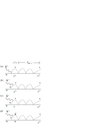
Figure 1: Diagrams for the microscopic mechanism of $\bar{K}^{*}N\to\Lambda^{*}\to\pi\Sigma^{*}$ calculated in the chiral unitary model.

Since we are considering first the $s$-wave coupling, the amplitude $-it_{l\bar{K}^{*}N}$ should be written as $-it_{l\bar{K}^{*}N}=g_{l\bar{K}^{*}N}\bm{S}^{\dagger}\cdot\bm{\epsilon}$, where $g_{l\bar{K}^{*}N}$ will be calculated later. We denote the total energy as $\sqrt{s}$, and consider the energy region close to the $\Lambda^{*}$ pole $\sqrt{s}\sim M_{\Lambda^{*}}$ with $M_{\Lambda^{*}}$ being the mass of the $\Lambda^{*}$ resonance. In this region, the chiral unitary amplitude $T_{ij}$ can be approximated by the Breit-Wigner propagator $T_{ij}\sim g_{\Lambda^{*}i}g_{\Lambda^{*}j}/(\sqrt{s}-M_{\Lambda^{*}})$ with coupling constants $g_{\Lambda^{*}i}$, where $i$ stands for the channels coupling to $\Lambda^{*}$. Then we have

$$-it_{\text{ChU}}\sim-ig_{\Lambda^{*}\pi\Sigma^{*}}\frac{i}{\sqrt{s}-M_{\Lambda^{*}}}\sum_{l}g_{\Lambda^{*}l}\,G_{l}\,g_{l\bar{K}^{*}N}\bm{S}^{\dagger}\cdot\bm{\epsilon}.$$ (4)

On the other hand, with the $s$-wave coupling Eq. (2), the resonance model for the amplitude $\bar{K}^{*}N\to\Lambda^{*}\to\pi\Sigma(1385)$ can be written as shown in Fig. 2,

$$-it_{\text{res}}=-ig_{\Lambda^{*}\pi\Sigma^{*}}\frac{i}{\sqrt{s}-M_{\Lambda^{*}}}g_{\Lambda^{*}\bar{K}^{*}N}\bm{S}^{\dagger}\cdot\bm{\epsilon},$$

where $g_{\Lambda^{*}\bar{K}^{*}N}$ is the $\Lambda^{*}\bar{K}^{*}N$ coupling constant that we are interested in. Hence comparing this amplitude with Eq. (4), we extract the $\Lambda^{*}\bar{K}^{*}N$ coupling as

$$g_{\Lambda^{*}\bar{K}^{*}N}=\sum_{l}g_{\Lambda^{*}l}\,G_{l}\,g_{l\bar{K}^{*}N}.$$ (5)

In the previous study Luis , the coupling constants $g_{\Lambda^{*}l}$ have been determined as

$$g_{\Lambda^{*}\pi\Sigma^{*}}=0.91,\quad g_{\Lambda^{*}\pi\Sigma}=-0.45,\quad g_{\Lambda^{*}\bar{K}N}=-0.54,$$ (6)

which well reproduce the partial decay widths of the $\Lambda(1520)$ resonance to these channels. In the following, we evaluate $G_{l}g_{l\bar{K}^{*}N}$ by calculating the diagrams in Fig. 1 one by one.

Figure 2: Diagram for the resonance dominance model of $\bar{K}^{*}N\to\Lambda^{*}\to\pi\Sigma^{*}$.

II.2 Computation of loop diagrams

Let us first consider the diagrams (a) and (b) in Fig. 1. The amplitudes for these diagrams $-it^{(a)}$ and $-it^{(b)}$ are related to each other through the gauge condition

$$(-it_{\mu}^{(a)}-it_{\mu}^{(b)})k^{\mu}=0,$$ (7)

where $-it^{(i)}\equiv-it^{(i)}_{\mu}\epsilon^{\mu}$ and $k^{\mu}$ is the momentum of the $\bar{K}^{*}$. First we consider the diagram (b). Utilizing the interaction Lagrangians given in appendix, the amplitude of, for instance, $\bar{K}^{*0}n\to\pi^{+}\Sigma^{*-}$ for the meson pole diagram (b) at tree level is written as

$$-it^{(b)}_{\pi^{-}\Sigma^{*+}\bar{K}^{*-}n}= \frac{1}{\sqrt{2}}ig\epsilon^{\mu}(2q_{\mu}-k_{\mu})\frac{i}{(q-k)^{2}-m_{K}^{2}}$$

$$\times\frac{1}{\sqrt{3}}\frac{g_{A}^{*}}{2f}\bm{S}^{{\dagger}}\cdot(\bm{q}-\bm{k}).$$ (8)

The momentum variables in Eq. (8) are assigned as shown in Fig. 3, $m_{K}$ is the mass of kaon, $g=-6.05$, $g_{A}^{*}=(D+F)\times 2.13$, $D+F=1.26$, $f=f_{\pi}=93$ MeV. In order to obtain the corresponding tree level amplitude for the contact diagram (a), $-it^{(a)}_{\pi^{-}\Sigma^{*+}\bar{K}^{*-}n}$, we first replace $\epsilon^{\mu}$ by $k^{\mu}$ in Eq. (8), set $q^{2}=m_{\pi}^{2}=M_{K}^{2}$ assuming the SU(3) limit (this manipulation is only for the purpose of determining the contact term) and set $\bm{q}=\bm{0}$. Then, the contact term has to be

$$-it^{(a)}_{\pi^{-}\Sigma^{*+}\bar{K}^{*-}n}=\frac{g}{\sqrt{2}}\frac{g_{A}^{*}}{2f}\frac{1}{\sqrt{3}}\bm{S}^{{\dagger}}\cdot\bm{\epsilon},$$

in order to satisfy Eq. (7).

We can repeat the same operation for other charge states. Writing the $\bar{K}^{*}N$ and $\pi\Sigma^{*}$ states in isospin basis (recalling that $|\,K^{*-}\,\rangle=-|\,1/2,-1/2\,\rangle$ and $|\,\pi^{+}\,\rangle=-|\,1,1\,\rangle$ in our convention), we find

$$-it^{(a)}_{\pi\Sigma^{*}\bar{K}^{*}N}=\frac{g}{2}\frac{g_{A}^{*}}{2f}\bm{S}^{{\dagger}}\cdot\bm{\epsilon},$$ (9)

after projecting over $I=0$. Inserting Eq. (9) into Eq. (3), we can now write

$$-it^{(a)}=(-iT_{\pi\Sigma^{*}\pi\Sigma^{*}})iG_{\pi\Sigma^{*}}\,g_{\pi\Sigma^{*}\bar{K}^{*}N}\,\bm{S}^{\dagger}\cdot\bm{\epsilon},$$ (10)

where $G_{\pi\Sigma^{*}}$ is the loop function involving the $\pi$ and the $\Sigma^{*}$:

$$G_{\pi\Sigma^{*}}(\sqrt{s})= i\int\frac{d^{4}q}{(2\pi)^{4}}\frac{1}{q^{2}-m_{\pi}^{2}+i\epsilon}$$

$$\times\frac{1}{\sqrt{s}-q^{0}-E_{\Sigma^{*}}+i\epsilon},$$

where $E_{\Sigma^{*}}(\bm{q})=\sqrt{M_{\Sigma^{*}}^{2}+\bm{q}^{2}}$ and the coupling constant is given by

$$g_{\pi\Sigma^{*}\bar{K}^{*}N}=\frac{1}{2}g\frac{g_{A}^{*}}{2f}.$$ (11)

Figure 3: Momentum assignment for the diagram (b) in Fig. 1.

On the other hand, we can also extract the $s$-wave component of the meson pole term from Eq. (8) after projecting over $I=0$, and we find

$$-it^{(b)}_{l\bar{K}^{*}N}=g_{\pi\Sigma^{*}\bar{K}^{*}N}\frac{2}{3}\frac{\bm{q}^{2}}{(q-k)^{2}-m_{K}^{2}}\bm{S}^{{\dagger}}\cdot\bm{\epsilon},$$ (12)

where the variable $\bm{q}$ should be included in the loop function. Therefore, the amplitude for this process can be expressed similarly as in Eq. (10) but with the meson-baryon loop function $G_{\pi\Sigma^{*}}$ replaced by the loop function with an additional factor, which is defined by

$$\tilde{G}_{\pi\Sigma^{*}K}(\sqrt{s},k)= i\int\frac{d^{4}q}{(2\pi)^{4}}\frac{\bm{q}^{2}}{(q-k)^{2}-m_{K}^{2}+i\epsilon}$$

$$\times\frac{1}{q^{2}-m_{\pi}^{2}+i\epsilon}\frac{1}{\sqrt{s}-q^{0}-E_{\Sigma^{*}}+i\epsilon}.$$

Finally, combining the contributions from $(a)$ and $(b)$, we obtain

$$-it^{(a)}-it^{(b)}= (-iT_{\pi\Sigma^{*}\pi\Sigma^{*}})i\left(G_{\pi\Sigma^{*}}+\frac{2}{3}\tilde{G}_{\pi\Sigma^{*}K}\right)$$

$$\times g_{\pi\Sigma^{*}\bar{K}^{*}N}\bm{S}^{\dagger}\cdot\bm{\epsilon}~{}.$$

We now evaluate the amplitude for the diagram (c) and (d) in Fig. 1. The structure of the first loop can be found from Fig. 4. Since we need the $d$-wave projection of the meson pole term to balance the $d$-wave $\bar{K}N\to\pi\Sigma^{*}$ amplitude in the loop, we study the amplitude in some detail. Using the interaction Lagrangians given in the appendix, the $I=0$ component of the tree level amplitude for (d), for instance, is given by

$$-it^{(d)}_{\bar{K}N\bar{K}^{*}N}= -3ig\frac{D+F}{2f}\epsilon^{\mu}(2q_{\mu}-k_{\mu})$$

$$\times\frac{i}{(q-k)^{2}-m_{\pi}^{2}}\bm{\sigma}\cdot(\bm{k}-\bm{q}).$$

The spin structure takes the form $(\bm{\epsilon}\cdot\bm{q})(\bm{\sigma}\cdot\bm{q})$, neglecting $\bm{k}$ which is assumed to be small. Now, the $d$-wave structure obtained from $\sigma_{i}q_{i}\epsilon_{j}q_{j}\to\sigma_{i}\epsilon_{j}(q_{i}q_{j}-\bm{q}^{2}\delta_{ij}/3)$ will combine with the $d$-wave structure coming from the $\bar{K}N\to\pi\Sigma^{*}$ vertex to produce a scalar quantity after the loop integration is performed. We write

$$\sigma_{i}\epsilon_{j}(q_{i}q_{j}-\tfrac{1}{3}\bm{q}^{2}\delta_{ij})=A\left[[\sigma\otimes\epsilon]_{\mu}^{2}\ Y_{2}(\hat{q})\right]_{0}^{0},$$ (13)

where $A$ is a constant. This indicates that the two vector operators $\sigma$ and $\epsilon$ combine to produce an operator of rank $2$, which couples to the spherical harmonic $Y_{2}(\hat{q})$ to produce a scalar. The right hand side can be written as

$$A \sum_{\mu}(-1)^{\mu}[\sigma\otimes\epsilon]_{\mu}^{2}\ Y_{2,-\mu}(\hat{q})$$

$$=A\sum_{\mu,\alpha}(-1)^{\mu}Y_{2,-\mu}(\hat{q})\ {\cal{C}}(1\ 1\ 2;\alpha,\mu-\alpha)\sigma_{\alpha}\epsilon_{\mu-\alpha}.$$

To find the value of $A$ we take the matrix element of both sides of Eq. (13) between the states $m$ and $m^{\prime}$ so that

$$\langle m|\sigma_{i} \epsilon_{j}\left(q_{i}q_{j}-\frac{1}{3}|\bm{q}|^{2}\delta_{ij}\right)|m^{\prime}\rangle$$

$$= A\sum_{\mu}(-1)^{\mu}\ Y_{2,-\mu}(\hat{q})\ \epsilon_{\mu-m+m^{\prime}}$$

$$\times{\cal{C}}(1\ 1\ 2;m-m^{\prime},\mu-m+m^{\prime})$$

$$\times{\cal{C}}\left(\frac{1}{2}\ 1\ \frac{1}{2};m^{\prime},m-m^{\prime}\right),$$ (14)

where we have used $\langle m|\sigma_{\alpha}|m^{\prime}\rangle=\sqrt{3}\ {\cal{C}}(\tfrac{1}{2}\ 1\ \tfrac{1}{2};m^{\prime},\alpha)$ with $m=m^{\prime}+\alpha$. Considering specific values of $m$ and $m^{\prime}$, we obtain

$$A=\sqrt{\frac{8\pi}{15}}\ \bm{q}^{2}.$$ (15)

Figure 4: Momentum and spin indices assignment for the loop diagram in (d) in Fig. 1.

Following Ref. Sarkar:2005ap , we now include the $\bar{K}N\to\pi\Sigma^{*}$ vertex given by

$$-it_{\bar{K}N\to\pi\Sigma^{*}}= -i\beta_{\bar{K}N}\ \bm{q}^{2}\ {\cal{C}}\left(\frac{1}{2}\ 2\ \frac{3}{2};m,M-m\right)$$

$$\times Y_{2,m-M}(\hat{q})(-1)^{M-m}\sqrt{4\pi},$$ (16)

so that the total spin structure of the loop shown in Fig. 4 is essentially given by

$$J= \sum_{m}\int\frac{d\Omega_{q}}{4\pi}\langle m|\sigma_{i}\epsilon_{j}\left(q_{i}q_{j}-\frac{1}{3}\bm{q}^{2}\delta_{ij}\right)|m^{\prime}\rangle$$

$$\times{\cal{C}}\left(\frac{1}{2}\ 2\ \frac{3}{2};m,M-m\right)Y_{2,m-M}(\hat{q})(-1)^{M-m}\sqrt{4\pi},$$

where we perform an average over the angular dependence in the integration over the loop momentum $q$. Using Eqs. (14) and (15) this can be written as

$$J= \sqrt{\frac{2}{3}}\bm{q}^{2}(-1)^{1-M+m^{\prime}}\ \epsilon_{m^{\prime}-M}\sum_{m}\ {\cal{C}}(\tfrac{1}{2}\ 1\ \tfrac{1}{2};m^{\prime},m-m^{\prime})\$$

$$\times{\cal{C}}(\tfrac{1}{2}\ 2\ \tfrac{3}{2};m,M-m){\cal{C}}(1\ 2\ 1;m-m^{\prime},M-m),$$

where we have used the well known relations

$$\int\ d\Omega_{q}\ Y_{2,-\mu}(\hat{q})\ Y_{2,m-M}(\hat{q})=(-1)^{\mu}\delta_{\mu,m-M},$$

and

$${\cal{C}}(1\ 1\ 2;m-m^{\prime},m^{\prime}-M)$$

$$= (-1)^{1-m+m^{\prime}}\sqrt{\frac{5}{3}}\ {\cal{C}}(1\ 2\ 1;m-m^{\prime},M-m).$$

The product of three Clebsch-Gordan coefficients is then combined into a single one with Racah coefficients, resulting in the identity

$$\sum_{m} {\cal{C}}\left(\frac{1}{2}\ 1\ \frac{1}{2};m^{\prime},m-m^{\prime}\right)\ {\cal{C}}\left(\frac{1}{2}\ 2\ \frac{3}{2};m,M-m\right)$$

$$\times{\cal{C}}(1\ 2\ 1;m-m^{\prime},M-m)$$

$$=-\sqrt{\frac{1}{2}}\ {\cal{C}}\left(\frac{1}{2}\ 1\ \frac{3}{2};m^{\prime},M-m^{\prime}\right),$$

so that, we finally have

$$J=\frac{1}{\sqrt{3}}\ \bm{q}^{2}\ \bm{S}^{\dagger}\cdot\bm{\epsilon}.$$ (17)

The above relation implies that for practical purposes we can replace in the first vertex $(\bm{\epsilon}\cdot\bm{q})(\bm{\sigma}\cdot\bm{q})$ by the simple form $\tfrac{1}{\sqrt{3}}\ \bm{q}^{2}\ \bm{S}^{\dagger}\cdot\bm{\epsilon}$ and for the second vertex the factor $\beta_{\bar{K}N}\bm{q}^{2}$ and continue with the formalism exactly as in $s$-wave. Putting everything together, the amplitude for the process shown in Fig. 1 (d) can be written as

$$-it^{(d)}=(-iT_{\pi\Sigma^{*}\bar{K}N})i\tilde{G}_{\bar{K}N\pi}\,g_{\bar{K}N\bar{K}^{*}N}\bm{S}^{\dagger}\cdot\bm{\epsilon},$$ (18)

which has the same form as Eq. (11). In the above equation, we have defined

$$g_{\bar{K}N\bar{K}^{*}N}=\sqrt{3}g\frac{D+F}{2f},$$

and

$$\tilde{G}_{\bar{K}N\pi}(\sqrt{s},k)= i\int\frac{d^{4}q}{(2\pi)^{4}}\ \frac{\bm{q}^{2}}{(q-k)^{2}-m_{\pi}^{2}+i\epsilon}\ \frac{\bm{q}^{2}}{q_{\text{on}}^{2}}$$

$$\times\frac{1}{q^{2}-m_{K}^{2}+i\epsilon}\frac{M_{N}}{E_{N}}\frac{1}{\sqrt{s}-q^{0}-E_{N}+i\epsilon},$$ (19)

with $q_{\text{on}}=\lambda^{1/2}(s,m_{N}^{2},m_{K}^{2})/2\sqrt{s}$. The factor $\bm{q}^{2}$ appearing in the vertex of Eq. (17) is kept in the loop. On the other hand, the amplitudes which we use for $\bar{K}N\to\pi\Sigma^{*}$ of Eq. (18) factorize the on shell value $q_{\text{on}}^{2}$. This is the reason for the factor $\frac{\bm{q}^{2}}{q_{\text{on}}^{2}}$ in Eq. (19) since in Eq. (18) we write explicitly $T_{\pi\Sigma^{*}\bar{K}N}$.

The amplitude for the process shown in Fig. 1 (c) can be evaluated in a similar way as described above. In this case we have

$$-it^{(c)}=(-iT_{\pi\Sigma^{*}\pi\Sigma})i\tilde{G}_{\pi\Sigma K}g_{\pi\Sigma\bar{K}^{*}N}\bm{S}^{\dagger}\cdot\bm{\epsilon},$$

where

$$g_{\pi\Sigma\bar{K}^{*}N}=\sqrt{2}g\frac{D-F}{2f},$$

with $D-F=0.33$ and $G_{\pi\Sigma K}$ given similarly as in Eq. (19) with the replacements $\pi\to K$ and $N\to\Sigma$.

Following Eq. (5), we thus obtain the coupling of the $\Lambda(1520)$ with $\bar{K}^{*}N$ as

$$g_{\Lambda^{*}\bar{K}^{*}N}(\sqrt{s},k)= g_{\Lambda^{*}\pi\Sigma^{*}}\left[G_{\pi\Sigma^{*}}(\sqrt{s})+\frac{2}{3}\tilde{G}_{\pi\Sigma^{*}K}(\sqrt{s},k)\right]$$

$$\times g_{\pi\Sigma^{*}\bar{K}^{*}N}+g_{\Lambda^{*}\pi\Sigma}\,\tilde{G}_{\pi\Sigma K}(\sqrt{s},k)\,g_{\pi\Sigma\bar{K}^{*}N}$$

$$+g_{\Lambda^{*}\bar{K}N}\,\tilde{G}_{\bar{K}N\pi}(\sqrt{s},k)\,g_{\bar{K}N\bar{K}^{*}N}.$$ (20)

III Results and discussions

III.1 Chiral unitary model

Before calculating Eq. (20), let us consider the momentum variables. Since Eq. (4) is valid close to the pole of the resonance, we choose $\sqrt{s}=1520$ MeV. For this $\sqrt{s}$, $\Lambda^{*}$ cannot decay into $\bar{K}^{*}(892)$ and $N(940)$. Here we assume that the $\bar{K}^{*}$ is off the mass shell with the nucleon being on-shell, which would be compatible with the $K^{*}$ $t$-channel exchange in $\Lambda^{*}$ photoproduction on the nucleon target. Then the energy of the $\bar{K}^{*}$ can be given by

$$k^{0}=\sqrt{s}-E_{N}(\bm{k})=\sqrt{s}-\sqrt{M_{N}^{2}+\bm{k}^{2}},$$

where we are in the center of mass frame. As we have seen, our formulation is consistent with $|\bm{k}|\sim 0$, where the $s$-wave interaction is dominant. If $|\bm{k}|=0$, we obtain $k^{0}=\sqrt{s}-M_{N}\sim 580$ MeV, which is the maximum energy of the $\bar{K}^{*}$ when the nucleon is on-shell.

In order to study the finite momentum effect and stability of the result, we vary the momentum $|\bm{k}|$ from zero to 400 MeV, and plot the real and imaginary parts as well as the absolute value of the $\Lambda^{*}\bar{K}^{*}N$ coupling constant in Fig. 5. For reference, we also plot the energy $k^{0}$ in the lower panel in Fig. 5. We observe that the result is stable against the momentum $|\bm{k}|$ up to $\sim 200$ MeV, where the $s$-wave coupling is expected to be dominant. Numerical values are

$$g_{\Lambda^{*}\bar{K}^{*}N}\sim 1.53+0.41i,\quad|g_{\Lambda^{*}\bar{K}^{*}N}|\sim 1.58.$$

The complex phase is the relative one to $g_{\Lambda^{*}\bar{K}N}=-0.45$ given in Eq. (6).

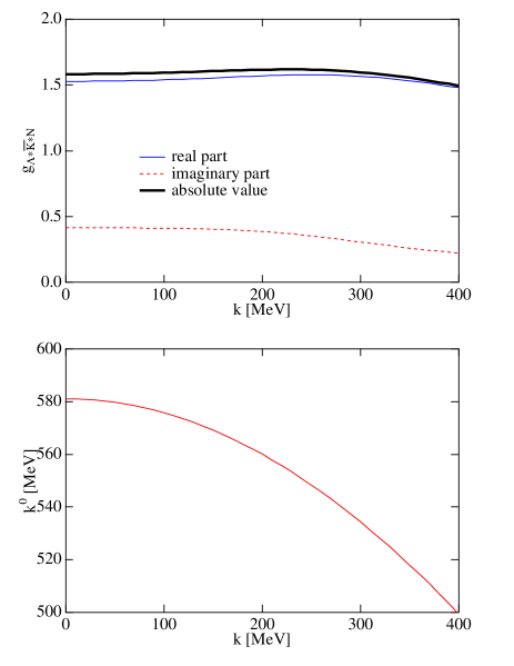
Figure 5: (Color online) Upper: Numerical results for the $\Lambda^{*}\bar{K}^{*}N$ coupling constant as a function of $K^{*}$ momentum $|\bm{k}|$ in the chiral unitary model. Thick solid line, thin solid line, and dashed line represent absolute value, real part, and imaginary part of the coupling constant, respectively. Lower: Energy of the $K^{*}$ as a function of $|\bm{k}|$, assuming the nucleon is on-shell.

Let us look at each component in detail. Substituting the numerical factors, Eq. (20) can be written as

$$g_{\Lambda^{*}\bar{K}^{*}N}\sim -0.042G_{\pi\Sigma^{*}}-0.028\tilde{G}_{\pi\Sigma^{*}K}$$

$$+0.0068\tilde{G}_{\pi\Sigma K}+0.038\tilde{G}_{\bar{K}N\pi}.$$ (21)

Note that the contribution from $\tilde{G}_{\pi\Sigma K}$ is factor 5 smaller than the others, due to the $D-F$ factor.

III.2 Quark model

In the quark model, $\Lambda(1520)$ resonance is a $p$-wave state of 70-dimensional representation of SU(6) Isgur:1978xj . In the spin-flavor group, it is a superposition of ${}^{2}\bm{1}$, ${}^{2}\bm{8}$, and ${}^{4}\bm{8}$. Here we use the notation ${}^{2S+1}D$, where $2S+1$ is the degeneracy of spin states and $D$ denotes a flavor representation. In the standard quark model, $\Lambda^{*}$ is dominated by the flavor singlet ${}^{2}\bm{1}$ with some mixture of ${}^{2}\bm{8}$; the spin quartet ${}^{4}\bm{8}$ has only a small fraction.

Such a wave function has been tested for the decay of $\Lambda^{*}\to\bar{K}N,\pi\Sigma$, and has been proven to work reasonably well Isgur:1978xj ; Hey:1974nc . For the decay to the chiral mesons, the matrix elements of the meson-quark interaction can be taken

$$\mathcal{L}_{mqq} =-ig_{mqq}\bar{q}\gamma_{5}\Phi q\to\tfrac{g_{mqq}}{2m_{q}}\chi^{\dagger}\bm{\sigma}\cdot\bm{\nabla}\Phi\chi~{},$$

where $\chi$ is a two-component spinor, and in the second line the non-relativistic approximation is performed. The SU(3) meson field is defined here by

$$\Phi=\left(\begin{array}[]{c c c}\pi^{0}+\frac{\eta}{\sqrt{3}}&\sqrt{2}\pi^{+}&\sqrt{2}K^{+}\\ \sqrt{2}\pi^{-}&\pi^{0}-\frac{\eta}{\sqrt{3}}&\sqrt{2}K^{0}\\ \sqrt{2}K^{-}&\sqrt{2}K^{0}&-\frac{2\eta}{\sqrt{3}}\end{array}\right)\,.$$ (25)

The meson-quark coupling constant $g_{mqq}\sim 2.6$ is determined from the $\pi NN$ coupling $g_{\pi NN}\sim 13$, and the constituent quark mass is taken as $330$ MeV for all $u,d,s$ quarks for simplicity. The use of a larger mass for $m_{s}$ will change slightly the SU(6) symmetric wave function such that the excitation of the strange quark will be easier than the excitation of the $u,d$ quarks. But we expect that the following results are not affected too much.

For the $\bar{K}^{*}$ (vector meson) coupling, we can use the interaction Lagrangian at the quark level

$$\mathcal{L}_{vqq}= g_{vqq}\bar{q}\gamma_{\mu}V^{\mu}q$$

$$\to -\frac{g_{vqq}}{\sqrt{2}m_{q}}\Bigl{\{}u^{\dagger}(i\bm{\nabla}-i\bm{\nabla})s$$

$$+\bm{\nabla}\times(u^{\dagger}\bm{\sigma}s)\Bigr{\}}\cdot\bm{\epsilon}(K^{*+})+\text{h.c.}\,,$$ (26)

where $\bm{\epsilon}(K^{*+})$ is the polarization vector of the $K^{*+}$, the quark flavor is indicated explicitly for the $\bar{K}^{*}$ coupling, and the $g_{vqq}\sim 3$ is determined by the empirical $\rho NN$ coupling strength. This Lagrangian of vector type coupling works well for baryon magnetic moments when the $\bar{K}^{*}$ is replaced by the photon after SU(3) rotation. For the $\rho NN$, however, the tensor coupling is slightly underestimated $g_{T}/g_{V}\sim 4$, as compared with the strong tensor coupling $g_{T}/g_{V}\sim 6$ Machleidt:1987hj . For the present study of qualitative analysis, however, we simply adopt the Lagrangian (26).

In order to extract the relevant coupling strength, we compute the two transverse helicity amplitudes,

$$a_{3/2} \equiv-\langle N(s_{z}=1/2),K^{*}(h=+1)|{\cal L}_{vqq}|\Lambda^{*}(s_{z}=3/2)\rangle$$

$$a_{1/2} \equiv-\langle N(s_{z}=-1/2),K^{*}(h=+1)|{\cal L}_{vqq}|\Lambda^{*}(s_{z}=1/2)\rangle\,.$$

Here $s_{z}$ represents the third component of spin and $h$ the helicity of the photon. In general, for a massive vector meson, there is another type of scalar or longitudinal one, which can be computed by the time component of the current. For the present purpose, however, the two transverse components are sufficient. They are then related to the multipole amplitudes by

$$E1 =-\frac{1}{2}a_{1/2}-\frac{\sqrt{3}}{2}a_{3/2}\,,$$

$$M2 =\frac{\sqrt{3}}{2}a_{1/2}-\frac{1}{2}a_{3/2}\,.$$

The quark model calculation is rather standard, and so we just show the final result:

$$E1 =-i\frac{3\sqrt{2}\sqrt{\alpha}}{m_{q}}g_{vqq}\left(1-\frac{\bm{k}^{2}}{6\alpha}\right)e^{-\bm{k}^{2}/6\alpha}\,,$$

$$M2 =-i\frac{\sqrt{6}\sqrt{\alpha}}{4m_{q}}g_{vqq}\frac{\bm{k}^{2}}{6\alpha}e^{-\bm{k}^{2}/6\alpha}\,,$$

where $\bm{k}$ is the momentum of $K^{*}$ and $\alpha$ is a harmonic oscillator parameter of the wave function of the non-relativistic quark model, which is related to the size of the system by

$$\langle r^{2}\rangle=3/\alpha\,.$$

The $\Lambda^{*}\bar{K}^{*}N$ coupling constant is then related to the $E1$ amplitude by an overall constant

$$g_{\Lambda^{*}\bar{K}N}=\frac{3}{\sqrt{6}}E1.$$ (27)

In the calculation, we consider a mixing of ${}^{2}\bm{1}$ and ${}^{2}\bm{8}$ states for $\Lambda(1520)$ as

$$|\Lambda(1520)\rangle=\cos\theta|^{2}\bm{1}\rangle+\sin\theta|^{2}\bm{8}\rangle\,.$$

In the Isgur-Karl model, the mixing angle was obtained $\theta\sim 0.4$ Isgur:1978xj . The result is shown in Fig. 6, where the coupling constant $g_{\Lambda^{*}\bar{K}^{*}N}$ is shown as a function of $K^{*}$ three-momentum $k$ for different mixing angles $\theta$. The quark model value, in contrast with that of the chiral unitary approach, is of order $g_{\Lambda^{*}\bar{K}^{*}N}\sim 10$. In particular, the value increases slightly as the mixing angle increases, which is a consequence of the interference between the two flavor states. The difference between the values of the chiral unitary model and the quark model is large, and it would be interesting to test the coupling by experiments. In reality, the physical resonance state may be a mixture of the two extreme schemes of the chiral unitary and the quark models. The coupling $g_{\Lambda^{*}\bar{K}^{*}N}$ could be used to investigate such a hybrid nature of the resonance.

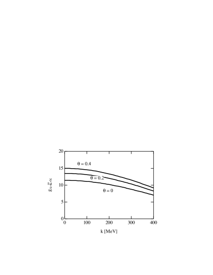
Figure 6: Numerical result for the $\Lambda^{*}\bar{K}^{*}N$ coupling constant as a function of $K^{*}$ momentum $k$ in the quark model, for different mixing angles $\theta$.

For completeness, we would like to mention the phenomenological analysis of the $g_{\Lambda^{*}\bar{K}^{*}N}$ coupling constant. In Ref. Titov:2005kf , the $g_{\Lambda^{*}\bar{K}^{*}N}$ is estimated from the $\Lambda^{*}$ photoproduction data Barber:1980zv . They fit the cross section at $E_{\gamma}=2.8$-$4.8$ GeV by a Regge trajectory of $K^{*}$ exchange, and match the amplitude at $E_{\gamma}=2.3$ GeV to the one calculated by the Born terms with the effective Lagrangian approach which includes the $g_{\Lambda^{*}\bar{K}^{*}N}$ in the $K^{*}$ $t$-channel exchange. The result in the present convention is

$$g_{\Lambda^{*}\bar{K}^{*}N}=+7.1\text{ or }-12.6,$$ (28)

where we denote the relative $\pm$ sign to $g_{\Lambda^{*}\bar{K}N}$. However, this conclusion depends on the assumption of the Regge trajectory of $K^{*}$ exchange, and the same data Barber:1980zv can be equally well reproduced with $g_{\Lambda^{*}\bar{K}^{*}N}=0$ in a different model Nam:2005uq , where the Kroll-Ruderman term plays a dominant role. In order to perform a precise phenomenological analysis, we need further experimental information of the $\Lambda^{*}$.

IV Summary and discussions

In this paper, we have studied the $\Lambda(1520)\bar{K}^{*}N$ coupling constant. The motivations are twofold: One is to offer a model estimation for the unknown coupling constant which is expected to be important in hyperon production reactions, and the other one is to test different types of models for baryon resonances. In the chiral unitary model the resonances are described as a meson baryon quasibound state which may indicate the importance of hadron-like correlations in hadron structure.

Since the coupling constant has not been calculated in the chiral unitary model before, we have shown here a detailed derivation. The resulting coupling constant $g_{\Lambda^{*}\bar{K}^{*}N}$ is expressed as a sum over contributions from various channels necessary for the formation of $\Lambda^{*}$. The actual number of the coupling $g_{\Lambda^{*}\bar{K}^{*}N}$ turned out to be of order 1-2, which is significantly smaller than the quark model value of order 10.

The difference in the results in two models should be a consequence of the difference of the model setup in various aspects. First, the quark model describes the $\Lambda^{*}$ as a three-quark system, while it is five-quark description in the chiral unitary model. Second, in the chiral unitary model, the $\Lambda^{*}$ is mainly a member of flavor $\bm{8}$, while in the quark model it is presumably dominated by the flavor singlet $\bm{1}$. Third, the wave function of the $\Lambda^{*}$ would be dominated by the $s$-wave component of $\pi\Sigma(1385)$, while it is a $p$-wave excitation in the quark model. Such differences in the internal structure should be reflected in the $\Lambda^{*}\bar{K}^{*}N$ coupling. If the actual $\Lambda(1520)$ has a mixed structure of the meson-baryon quasibound state and the three-quark state, the relevant coupling constant will be an intermediate value.

Since we have no experimental information of the coupling it would be very interesting to have the experimental value. Photoproduction reactions such as $\gamma N\to\Lambda^{*}K$ and $\gamma N\to\Lambda^{*}K^{*}$ may discriminate the coupling constant. In the $K$ production case, comparison between proton target and neutron target will be useful, since the $K$ exchange and contact terms are absent for the neutron target Nam:2005uq . As a consequence, the $t$-channel behavior is dominated by the $K^{*}$ exchange, so that the angular dependence is very sensitive to the strength of the $\Lambda^{*}\bar{K}^{*}N$ coupling constant. Hence, the angular dependence of the cross section ratio of proton and neutron will give us the information of the coupling constant of interest. It is also interesting to investigate the $\gamma p\to\Lambda^{*}K$ and $\gamma p\to\Lambda^{*}K^{*}$ reactions with $\Lambda^{*}$ going forward, which is naively dominated by the $u$-channel diagram. When the exchanged particle is the $\Lambda^{*}$, the cross section ratio of the $K$ production and the $K^{*}$ production provides the ratio of the coupling constants $\Lambda^{*}\bar{K}N$ and $\Lambda^{*}\bar{K}^{*}N$. Information from such experiments as well as theoretical comparison would provide further understanding of the resonance structure.

Appendix A Lagrangians and conventions

Here we summarize the chiral Lagrangians which are used in the present analysis. The coupling of vector meson and pseudoscalar mesons is given by

$${\cal{L}}_{1}=-i\frac{g}{\sqrt{2}}\text{Tr}(V^{\mu}[\partial_{\mu}P,P]),$$ (29)

with $g=-6.05$ and the Yukawa coupling of ground state baryon is given by

$${\cal{L}}_{2}=\text{Tr}\left(\frac{D}{2}\bar{B}\gamma^{\mu}\gamma^{5}\{u_{\mu},B\}+\frac{F}{2}\bar{B}\gamma^{\mu}\gamma^{5}[u_{\mu},B]\right),$$ (30)

with standard notations given in Refs. Ecker:1995gg ; Pich:1995bw ; Bernard:1995dp . The coupling constants are such that $D+F=1.26$ and $D-F=0.33$. With these Lagrangians, we obtain the amplitudes for the $t$-channel meson exchange processes $\bar{K}^{*}(k)+\pi(q-k)\to\bar{K}(q)$ and $N\to\pi(q-k)+N$

$$-it_{1}= -i\alpha\frac{g}{2}(2q-k)_{\mu}\epsilon^{\mu},$$

$$-it_{2}= \left(\beta\frac{D+F}{2f}+\gamma\frac{D-F}{2f}\right)\bm{\sigma}\cdot(\bm{q}-\bm{k}),$$

with suitable SU(3) coefficients $\alpha$, $\beta$, and $\gamma$. The Yukawa coupling of $\Sigma^{*}\to M_{i}(q-k)+B_{i}$ is similarly given by

$$-it_{3}=c_{i}\frac{12}{5}\frac{g_{A}^{*}}{2f}\bm{S}\cdot(\bm{q}-\bm{k}).$$

with $g_{A}^{*}=(D+F)\times 2.13$ where the numerical factor comes from $f_{\pi N\Delta}=2.13f_{\pi NN}$. SU(3) coefficients $c_{i}$ are tabulated in Refs. Jido:2002zk ; Hyodo:2004vt .

References

- (1) LEPS Collaboration, T. Nakano et al., Phys. Rev. Lett. 91, 012002 (2003).
- (2) R. L. Jaffe, Phys. Rep. 409, 1 (2005).
- (3) R. L. Jaffe, Phys. Rev. D 72, 074508 (2005).
- (4) R. H. Dalitz and S. F. Tuan, Ann. Phys. (NY) 10, 307 (1960).
- (5) B. K. Jennings, Phys. Lett. B176, 229 (1986).
- (6) N. Kaiser, P. B. Siegel, and W. Weise, Nucl. Phys. A594, 325 (1995).
- (7) E. Oset and A. Ramos, Nucl. Phys. A635, 99 (1998).
- (8) D. Jido, J. A. Oller, E. Oset, A. Ramos, and U. G. Meissner, Nucl. Phys. A725, 181 (2003).
- (9) T. Hyodo, A. Hosaka, E. Oset, A. Ramos, and M. J. Vicente Vacas, Phys. Rev. C 68, 065203 (2003).
- (10) V. K. Magas, E. Oset, and A. Ramos, Phys. Rev. Lett. 95, 052301 (2005).
- (11) E. E. Kolomeitsev and M. F. M. Lutz, Phys. Lett. B585, 243 (2004).
- (12) S. Sarkar, E. Oset, and M. J. Vicente Vacas, Nucl. Phys. A750, 294 (2005).
- (13) S. Sarkar, E. Oset, and M. J. Vicente Vacas, Phys. Rev. C 72, 015206 (2005).
- (14) L. Roca, S. Sarkar, V. K. Magas, and E. Oset, submitted to Phys. Rev. C.
- (15) S. Sarkar, L. Roca, E. Oset, V. K. Magas, and M. J. V. Vacas, nucl-th/0511062.
- (16) D. P. Barber et al., Z. Phys. C 7, 17 (1980).
- (17) A. Sibirtsev, J. Haidenbauer, S. Krewald, U.-G. Meissner, and A. W. Thomas, hep-ph/0509145.
- (18) S.-I. Nam, A. Hosaka, and H.-Ch. Kim, Phys. Rev. D 71, 114012 (2005).
- (19) A. I. Titov, B. Kampfer, S. Date, and Y. Ohashi, Phys. Rev. C 72, 035206 (2005).
- (20) T. E. O. Ericson and W. Weise, Pions and Nuclei (Clarendon press, Oxford, U.K., 1988).
- (21) N. Isgur and G. Karl, Phys. Rev. D 18, 4187 (1978).
- (22) A. J. G. Hey, P. J. Litchfield and R. J. Cashmore, Nucl. Phys. B95, 516 (1975).
- (23) R. Machleidt, K. Holinde and C. Elster, Phys. Rep. 149, 1 (1987).
- (24) G. Ecker, Prog. Part. Nucl. Phys. 35, 1 (1995).
- (25) A. Pich, Rep. Prog. Phys. 58, 563 (1995).
- (26) V. Bernard, N. Kaiser, and U.-G. Meissner, Int. J. Mod. Phys. E4, 193 (1995).
- (27) D. Jido, E. Oset, and A. Ramos, Phys. Rev. C 66, 055203 (2002).
- (28) T. Hyodo, A. Hosaka, M. J. Vicente Vacas, and E. Oset, Phys. Lett. B593, 75 (2004).