Abstract

In this article, we calculate the scalar form-factor of the proton in the framework of the light-cone QCD sum rules approach with the three valence quark light-cone distribution amplitudes up to twist-6, and observe the scalar form-factor $\sigma(t=-Q^{2})$ at intermediate and large momentum transfers $Q^{2}>2GeV^{2}$ has significant contributions from the end-point (or soft) terms. The numerical values for the $\sigma(t=-Q^{2})$ are compatible with the calculations from the chiral quark model and lattice QCD at the region $Q^{2}>2GeV^{2}$.

PACS : 12.38.-t, 14.20.Dh, 13.40.Gp

Key Words: Sigma term, Light-cone QCD sum rules, Scalar form-factor

1 Introduction

The pion-nucleon sigma-term $\Sigma_{\pi N}$ measures the nucleon mass shift away from the chiral limit and is particularly suited to test our understanding of the mechanism of the spontaneous and explicit chiral symmetry breaking in QCD due to the non-zero $u$, $d$ quark masses ( For an elegant review of the earlier works, one can consult Ref.[1] ). The precise knowledge of the values of the $\Sigma_{\pi N}$ is of great importance for many phenomenological applications, for example, the $\Sigma_{\pi N}$ enters the counting rates in searching for the Higgs boson [2], supersymmetric particles [3] and dark matter [4, 5]. However, no experimental method can be used to measure the $\Sigma_{\pi N}$ directly. The low energy theorem relates the nucleon scalar form-factor $\sigma(t)$ to the isospin-even $\pi N$ scattering amplitude $D^{+}(\nu,t)$ at the un-physical Cheng-Dashen point, $\nu=0,t=2m_{\pi}^{2}$ [6]. The Cheng-Dashen point lies outside the physical $\pi N$ scattering region, we have to extrapolate the experimental $\bar{D}^{+}$ amplitude to obtain the $\Sigma_{\pi N}$ with the general techniques of the dispersion relation and partial-waves analysis, the bar over $\bar{D}^{+}$ indicates that the pseudo-vector Born term has been subtracted. Earlier analysis performed by Koch [7] and Gasser, Leutwyler, Sainio [8] gave the canonical value for the $\sigma(2m_{\pi}^{2})$, $\sigma(2m_{\pi}^{2})\approx 60\,{\rm MeV}$, however, the recent analysis of the $\pi N$ scattering data supports the values $\Sigma_{\pi N}=79\pm 7$ MeV [9]. Although there have been a lot of works on the pion-nucleon sigma-term, for example, chiral perturbation theory [10, 11, 12], lattice QCD [13, 14, 15, 16], various chiral quark models [17, 18, 19, 20], or Schwinger-Dyson equation [21], the value of the sigma term remains a puzzle.

In this article, we calculate the scalar form-factor $\sigma(t)$ of the proton in the framework of the light-cone sum rules (LCSR) [22, 25] which combine the standard techniques of the QCD sum rules with the conventional parton distribution amplitudes describing the hard exclusive processes [23]. In the LCSR approach, the short-distance operator product expansion with the vacuum condensates of increasing dimensions is replaced by the light-cone expansion with the distribution amplitudes (which correspond to the sum of an infinite series of operators with the same twist) of increasing twists to parameterize the non-perturbative QCD vacuum, while the contributions from the hard re-scattering can be correctly incorporated as the $O(\alpha_{s})$ corrections [24]. In recent years, there have been a lot of applications of the LCSR to the mesons, for example, the form-factors, strong coupling constants and hadronic matrix elements [25], the applications to the baryons are cumbersome and only the nucleon electromagnetic form-factors [26] and the weak decay $\Lambda_{b}\to p\ell\nu_{\ell}$ [27] are studied, the higher twists distribution amplitudes for the baryons were not available until recently [29].

The article is arranged as follows: we derive the light-cone sum rules for the scalar form-factor $\sigma(t)$ of the proton in section II; in section III, numerical results and discussion; section VI is reserved for conclusion.

2 Light-cone sum rules for the scalar form-factor

In the following, we write down the two-point correlation function $\Pi(P,q)$ in the framework of the LCSR approach,

$$\Pi(P,q)=i\int d^{4}x\,e^{iq\cdot x}\langle 0|T\left\{\eta(0)J(x)\right\}|P\rangle,$$ (1)

with the scalar current

$$J(x)=\bar{u}(x)u(x)+\bar{d}(x)d(x),$$ (2)

and the baryon current [28]

$$\eta(0) = \epsilon^{ijk}\left[u^{i}(0)C\!\not\!{z}u^{j}(0)\right]\,\gamma_{5}\!\not\!{z}d^{k}(0)\,,$$

$$\langle 0|\eta(0)|P\rangle = f_{\rm N}\,(P\cdot z)\!\not\!{z}N(P)\,,$$ (3)

here $z$ is a light-cone vector, $z^{2}=0$, and the $f_{N}$ is the coupling constant for the leading twist distribution amplitude [30]. At the large Euclidean momenta ${P^{\prime}}^{2}=(P-q)^{2}$ and $q^{2}=-Q^{2}$, the correlation function $\Pi(P,q)$ can be calculated in perturbation theory. In calculation, we need the following light-cone expanded quark propagator [31],

$$S(x) = \frac{i\Gamma(d/2)\not\!x}{2\pi^{2}(-x^{2})^{d/2}}$$ (4)

$$+ \frac{i\Gamma(d/2-1)}{16\pi^{2}(-x^{2})^{d/2-1}}\int\limits_{0}^{1}dv\Big{\{}(1-v)\not\!x\sigma_{\mu\nu}G^{\mu\nu}(vx)+v\sigma_{\mu\nu}G^{\mu\nu}(vx)\!\not\!x\Big{\}}+...,$$

where $G_{\mu\nu}=g_{s}G_{\mu\nu}^{a}(\lambda^{a}/2)$ is the gluon field strength tensor and $d$ is the space-time dimension. The contributions proportional to the $G_{\mu\nu}$ can give rise to four-particle (and five-particle) nucleon distribution amplitudes with a gluon or quark-antiquark pair in addition to the three valence quarks, their corrections are usually not expected to play any significant roles [32] and neglected here [26, 27]. Employ the light-cone quark propagator in the correlation function $\Pi(P,q)$, we obtain

$$\Pi(P,q) = i\int d^{4}x\,\frac{e^{iq\cdot x}}{2\pi^{2}x^{4}}\left\{2(C\!\not\!{z}\!\not\!{x})^{\alpha\beta}(\gamma_{5}\!\not\!{z})^{\gamma}\epsilon^{ijk}\langle 0|T\left\{u^{i}_{\alpha}(0)u^{j}_{\beta}(x)d^{k}_{\gamma}(0)\right\}|P\rangle\right.$$ (5)

$$\left.+(C\!\not\!{z})^{\alpha\beta}(\gamma_{5}\!\not\!{z}\!\not\!{x})^{\gamma}\epsilon^{ijk}\langle 0|T\left\{u^{i}_{\alpha}(0)u^{j}_{\beta}(0)d^{k}_{\gamma}(x)\right\}|P\rangle\right\}\,.$$

In the light-cone limit $x^{2}\to 0$, the remaining three-quark operator sandwiched between the proton state and the vacuum can be written in terms of the nucleon distribution amplitudes [30, 28, 29]. It is obviously that if we only take into account the three valence quark component of the distribution amplitudes, the correlation function $i\int d^{4}x\,e^{iq\cdot x}\langle 0|T\left\{\eta(0)\bar{s}(x)s(x)\right\}|P\rangle$ must be zero, i.e. the strange-component of the scalar form-factor $\langle P^{\prime}|\bar{s}(0)s(0)|P\rangle=0$; if the strange-component of the $\pi N$ sigma term manifests itself, the distribution amplitudes with additional valence gluons and quark-antiquark pairs must play significant roles. The three valence quark components of the nucleon distribution amplitudes are defined by the matrix element,

$$4\langle 0|\epsilon^{ijk}u_{\alpha}^{i}(a_{1}x)u_{\beta}^{j}(a_{2}x)u_{\gamma}^{k}(a_{3}x)|P\rangle=\mathcal{S}_{1}MC_{\alpha\beta}(\gamma_{5}N)_{\gamma}+\mathcal{S}_{2}M^{2}C_{\alpha\beta}(\hbox to0.0pt{/\hss}x\gamma_{5}N)_{\gamma}$$

$${}+\mathcal{P}_{1}M(\gamma_{5}C)_{\alpha\beta}N_{\gamma}+\mathcal{P}_{2}M^{2}(\gamma_{5}C)_{\alpha\beta}(\hbox to0.0pt{/\hss}xN)_{\gamma}+(\mathcal{V}_{1}+\frac{x^{2}M^{2}}{4}\mathcal{V}_{1}^{M})(\hbox to0.0pt{/\hss}PC)_{\alpha\beta}(\gamma_{5}N)_{\gamma}$$

$${}+\mathcal{V}_{2}M(\hbox to0.0pt{/\hss}PC)_{\alpha\beta}(\hbox to0.0pt{/\hss}x\gamma_{5}N)_{\gamma}+\mathcal{V}_{3}M(\gamma_{\mu}C)_{\alpha\beta}(\gamma^{\mu}\gamma_{5}N)_{\gamma}+\mathcal{V}_{4}M^{2}(\hbox to0.0pt{/\hss}xC)_{\alpha\beta}(\gamma_{5}N)_{\gamma}$$

$${}+\mathcal{V}_{5}M^{2}(\gamma_{\mu}C)_{\alpha\beta}(i\sigma^{\mu\nu}x_{\nu}\gamma_{5}N)_{\gamma}+\mathcal{V}_{6}M^{3}(\hbox to0.0pt{/\hss}xC)_{\alpha\beta}(\hbox to0.0pt{/\hss}x\gamma_{5}N)_{\gamma}$$

$${}+(\mathcal{A}_{1}+\frac{x^{2}M^{2}}{4}\mathcal{A}_{1}^{M})(\hbox to0.0pt{/\hss}P\gamma_{5}C)_{\alpha\beta}N_{\gamma}+\mathcal{A}_{2}M(\hbox to0.0pt{/\hss}P\gamma_{5}C)_{\alpha\beta}(\hbox to0.0pt{/\hss}xN)_{\gamma}+\mathcal{A}_{3}M(\gamma_{\mu}\gamma_{5}C)_{\alpha\beta}(\gamma^{\mu}N)_{\gamma}$$

$${}+\mathcal{A}_{4}M^{2}(\hbox to0.0pt{/\hss}x\gamma_{5}C)_{\alpha\beta}N_{\gamma}+\mathcal{A}_{5}M^{2}(\gamma_{\mu}\gamma_{5}C)_{\alpha\beta}(i\sigma^{\mu\nu}x_{\nu}N)_{\gamma}+\mathcal{A}_{6}M^{3}(\hbox to0.0pt{/\hss}x\gamma_{5}C)_{\alpha\beta}(\hbox to0.0pt{/\hss}xN)_{\gamma}$$

$${}+(\mathcal{T}_{1}+\frac{x^{2}M^{2}}{4}\mathcal{T}_{1}^{M})(P^{\nu}i\sigma_{\mu\nu}C)_{\alpha\beta}(\gamma^{\mu}\gamma_{5}N)_{\gamma}+\mathcal{T}_{2}M(x^{\mu}P^{\nu}i\sigma_{\mu\nu}C)_{\alpha\beta}(\gamma_{5}N)_{\gamma}$$

$${}+\mathcal{T}_{3}M(\sigma_{\mu\nu}C)_{\alpha\beta}(\sigma^{\mu\nu}\gamma_{5}N)_{\gamma}+\mathcal{T}_{4}M(P^{\nu}\sigma_{\mu\nu}C)_{\alpha\beta}(\sigma^{\mu\rho}x_{\rho}\gamma_{5}N)_{\gamma}$$

$${}+\mathcal{T}_{5}M^{2}(x^{\nu}i\sigma_{\mu\nu}C)_{\alpha\beta}(\gamma^{\mu}\gamma_{5}N)_{\gamma}+\mathcal{T}_{6}M^{2}(x^{\mu}P^{\nu}i\sigma_{\mu\nu}C)_{\alpha\beta}(\hbox to0.0pt{/\hss}x\gamma_{5}N)_{\gamma}$$

$${}+\mathcal{T}_{7}M^{2}(\sigma_{\mu\nu}C)_{\alpha\beta}(\sigma^{\mu\nu}\hbox to0.0pt{/\hss}x\gamma_{5}N)_{\gamma}+\mathcal{T}_{8}M^{3}(x^{\nu}\sigma_{\mu\nu}C)_{\alpha\beta}(\sigma^{\mu\rho}x_{\rho}\gamma_{5}N)_{\gamma}\,\,.$$ (6)

The calligraphic distribution amplitudes do not have definite twist and can be related to the ones with definite twist as

$$\mathcal{S}_{1}=S_{1},\hskip 22.76228pt2P\cdot x\mathcal{S}_{2}=S_{1}-S_{2},$$

$$\mathcal{P}_{1}=P_{1},\hskip 22.76228pt2P\cdot x\mathcal{P}_{2}=P_{1}-P_{2}$$

for the scalar and pseudo-scalar distribution amplitudes,

$$\mathcal{V}_{1}=V_{1},\hskip 68.28644pt2P\cdot x\mathcal{V}_{2}=V_{1}-V_{2}-V_{3},$$

$$2\mathcal{V}_{3}=V_{3},\hskip 62.59596pt4P\cdot x\mathcal{V}_{4}=-2V_{1}+V_{3}+V_{4}+2V_{5},$$

$$4P\cdot x\mathcal{V}_{5}=V_{4}-V_{3},\hskip 14.22636pt(2P\cdot x)^{2}\mathcal{V}_{6}=-V_{1}+V_{2}+V_{3}+V_{4}+V_{5}-V_{6}$$

for the vector distribution amplitudes,

$$\mathcal{A}_{1}=A_{1},\hskip 68.28644pt2P\cdot x\mathcal{A}_{2}=-A_{1}+A_{2}-A_{3},$$

$$2\mathcal{A}_{3}=A_{3},\hskip 62.59596pt4P\cdot x\mathcal{A}_{4}=-2A_{1}-A_{3}-A_{4}+2A_{5},$$

$$4P\cdot x\mathcal{A}_{5}=A_{3}-A_{4},\hskip 14.22636pt(2P\cdot x)^{2}\mathcal{A}_{6}=A_{1}-A_{2}+A_{3}+A_{4}-A_{5}+A_{6}$$

for the axial vector distribution amplitudes, and

$$\mathcal{T}_{1}=T_{1},\hskip 109.54327pt2P\cdot x\mathcal{T}_{2}=T_{1}+T_{2}-2T_{3},$$

$$2\mathcal{T}_{3}=T_{7},\hskip 104.70593pt2P\cdot x\mathcal{T}_{4}=T_{1}-T_{2}-2T_{7},$$

$$2P\cdot x\mathcal{T}_{5}=-T_{1}+T_{5}+2T_{8},\hskip 14.22636pt(2P\cdot x)^{2}\mathcal{T}_{6}=2T_{2}-2T_{3}-2T_{4}+2T_{5}+2T_{7}+2T_{8},$$

$$4P\cdot x\mathcal{T}_{7}=T_{7}-T_{8},\hskip 54.06006pt(2P\cdot x)^{2}\mathcal{T}_{8}=-T_{1}+T_{2}+T_{5}-T_{6}+2T_{7}+2T_{8}$$

for the tensor distribution amplitudes. The distribution amplitudes $F=V_{i}$, $A_{i}$, $T_{i}$, $S_{i}$, $P_{i}$ can be represented as

$$F(a_{i}p\cdot x)=\int\mathcal{D}xe^{-ip\cdot x\Sigma_{i}x_{i}a_{i}}F(x_{i})\;,$$ (7)

with

$$\mathcal{D}x=dx_{1}dx_{2}dx_{3}\delta(x_{1}+x_{2}+x_{3}-1).$$

Those light-cone distribution amplitudes are scale dependent and can be expanded with the conformal operators, to the next-to-leading conformal spin accuracy, we obtain [29],

$$V_{1}(x_{i},\mu) = 120x_{1}x_{2}x_{3}[\phi_{3}^{0}(\mu)+\phi_{3}^{+}(\mu)(1-3x_{3})],$$

$$V_{2}(x_{i},\mu) = 24x_{1}x_{2}[\phi_{4}^{0}(\mu)+\phi_{3}^{+}(\mu)(1-5x_{3})],$$

$$V_{3}(x_{i},\mu) = 12x_{3}\{\psi_{4}^{0}(\mu)(1-x_{3})+\psi_{4}^{-}(\mu)[x_{1}^{2}+x_{2}^{2}-x_{3}(1-x_{3})]$$

$$+\psi_{4}^{+}(\mu)(1-x_{3}-10x_{1}x_{2})\},$$

$$V_{4}(x_{i},\mu) = 3\{\psi_{5}^{0}(\mu)(1-x_{3})+\psi_{5}^{-}(\mu)[2x_{1}x_{2}-x_{3}(1-x_{3})]$$

$$+\psi_{5}^{+}(\mu)[1-x_{3}-2(x_{1}^{2}+x_{2}^{2})]\},$$

$$V_{5}(x_{i},\mu) = 6x_{3}[\phi_{5}^{0}(\mu)+\phi_{5}^{+}(\mu)(1-2x_{3})],$$

$$V_{6}(x_{i},\mu) = 2[\phi_{6}^{0}(\mu)+\phi_{6}^{+}(\mu)(1-3x_{3})],$$

$$A_{1}(x_{i},\mu) = 120x_{1}x_{2}x_{3}\phi_{3}^{-}(\mu)(x_{2}-x_{1}),$$

$$A_{2}(x_{i},\mu) = 24x_{1}x_{2}\phi_{4}^{-}(\mu)(x_{2}-x_{1}),$$

$$A_{3}(x_{i},\mu) = 12x_{3}(x_{2}-x_{1})\{(\psi_{4}^{0}(\mu)+\psi_{4}^{+}(\mu))+\psi_{4}^{-}(\mu)(1-2x_{3})\},$$

$$A_{4}(x_{i},\mu) = 3(x_{2}-x_{1})\{-\psi_{5}^{0}(\mu)+\psi_{5}^{-}(\mu)x_{3}+\psi_{5}^{+}(\mu)(1-2x_{3})\},$$

$$A_{5}(x_{i},\mu) = 6x_{3}(x_{2}-x_{1})\phi_{5}^{-}(\mu)$$

$$A_{6}(x_{i},\mu) = 2(x_{2}-x_{1})\phi_{6}^{-}(\mu),$$

$$T_{1}(x_{i},\mu) = 120x_{1}x_{2}x_{3}[\phi_{3}^{0}(\mu)+\frac{1}{2}(\phi_{3}^{-}-\phi_{3}^{+})(\mu)(1-3x_{3})],$$

$$T_{2}(x_{i},\mu) = 24x_{1}x_{2}[\xi_{4}^{0}(\mu)+\xi_{4}^{+}(\mu)(1-5x_{3})],$$

$$T_{3}(x_{i},\mu) = 6x_{3}\{(\xi_{4}^{0}+\phi_{4}^{0}+\psi_{4}^{0})(\mu)(1-x_{3})+(\xi_{4}^{-}+\phi_{4}^{-}-\psi_{4}^{-})(\mu)[x_{1}^{2}+x_{2}^{2}-x_{3}(1-x_{3})]$$

$$+(\xi_{4}^{+}+\phi_{4}^{+}+\psi_{4}^{+})(\mu)(1-x_{3}-10x_{1}x_{2})\},$$

$$T_{4}(x_{i},\mu) = \frac{3}{2}\{(\xi_{5}^{0}+\phi_{5}^{0}+\psi_{5}^{0})(\mu)(1-x_{3})+(\xi_{5}^{-}+\phi_{5}^{-}-\psi_{5}^{-})(\mu)[2x_{1}x_{2}-x_{3}(1-x_{3})]$$

$$+(\xi_{5}^{+}+\phi_{5}^{+}+\psi_{5}^{+})(\mu)(1-x_{3}-2(x_{1}^{2}+x_{2}^{2}))\},$$

$$T_{5}(x_{i},\mu) = 6x_{3}[\xi_{5}^{0}(\mu)+\xi_{5}^{+}(\mu)(1-2x_{3})],$$

$$T_{6}(x_{i},\mu) = 2[\phi_{6}^{0}(\mu)+\frac{1}{2}(\phi_{6}^{-}-\phi_{6}^{+})(\mu)(1-3x_{3})],$$

$$T_{7}(x_{i},\mu) = 6x_{3}\{(-\xi_{4}^{0}+\phi_{4}^{0}+\psi_{4}^{0})(\mu)(1-x_{3})+(-\xi_{4}^{-}+\phi_{4}^{-}-\psi_{4}^{-})(\mu)[x_{1}^{2}+x_{2}^{2}-x_{3}(1-x_{3})]$$

$$+(-\xi_{4}^{+}+\phi_{4}^{+}+\psi_{4}^{+})(\mu)(1-x_{3}-10x_{1}x_{2})\},$$

$$T_{8}(x_{i},\mu) = \frac{3}{2}\{(-\xi_{5}^{0}+\phi_{5}^{0}+\psi_{5}^{0})(\mu)(1-x_{3})+(-\xi_{5}^{-}+\phi_{5}^{-}-\psi_{5}^{-})(\mu)[2x_{1}x_{2}-x_{3}(1-x_{3})]$$

$$+(-\xi_{5}^{+}+\phi_{5}^{+}+\psi_{5}^{+})(\mu)(1-x_{3}-2(x_{1}^{2}+x_{2}^{2}))\},$$

$$S_{1}(x_{i},\mu) = 6x_{3}(x_{2}-x_{1})\left[(\xi_{4}^{0}+\phi_{4}^{0}+\psi_{4}^{0}+\xi_{4}^{+}+\phi_{4}^{+}+\psi_{4}^{+})(\mu)+(\xi_{4}^{-}+\phi_{4}^{-}-\psi_{4}^{-})(\mu)(1-2x_{3})\right]\,,$$

$$S_{2}(x_{i},\mu) = \frac{3}{2}(x_{2}-x_{1})\left[-\left(\psi_{5}^{0}+\phi_{5}^{0}+\xi_{5}^{0}\right)(\mu)+\left(\xi_{5}^{-}+\phi_{5}^{-}-\psi_{5}^{0}\right)(\mu)x_{3}\right.$$

$$\left.+\left(\xi_{5}^{+}+\phi_{5}^{+}+\psi_{5}^{0}\right)(\mu)(1-2x_{3})\right]\,,$$

$$P_{1}(x_{i},\mu) = 6x_{3}(x_{2}-x_{1})\left[(\xi_{4}^{0}-\phi_{4}^{0}-\psi_{4}^{0}+\xi_{4}^{+}-\phi_{4}^{+}-\psi_{4}^{+})(\mu)+(\xi_{4}^{-}-\phi_{4}^{-}+\psi_{4}^{-})(\mu)(1-2x_{3})\right]\,,$$

$$P_{2}(x_{i},\mu) = \frac{3}{2}(x_{2}-x_{1})\left[\left(\psi_{5}^{0}+\psi_{5}^{0}-\xi_{5}^{0}\right)(\mu)+\left(\xi_{5}^{-}-\phi_{5}^{-}+\psi_{5}^{0}\right)(\mu)x_{3}\right.$$ (8)

$$\left.+\left(\xi_{5}^{+}-\phi_{5}^{+}-\psi_{5}^{0}\right)(\mu)(1-2x_{3})\right]\,.$$

The $V_{1}$, $A_{1}$ and $T_{1}$ are leading twist-3 distribution amplitudes; the $S_{1}$, $P_{1}$, $V_{2}$, $V_{3}$, $A_{2}$, $A_{3}$, $T_{2}$, $T_{3}$ and $T_{7}$ are twist-4 distribution amplitudes; the $S_{2}$, $P_{2}$, $V_{4}$, $V_{5}$, $A_{4}$, $A_{5}$, $T_{4}$, $T_{5}$ and $T_{8}$ are twist-5 distribution amplitudes; while the twist-6 distribution amplitudes are the $V_{6}$, $A_{6}$ and $T_{6}$. Those parameters $\phi_{3}^{0}$, $\phi_{6}^{0}$, $\phi_{4}^{0}$, $\phi_{5}^{0}$, $\xi_{4}^{0}$, $\xi_{5}^{0}$, $\psi_{4}^{0}$, $\psi_{5}^{0}$, $\phi_{3}^{-}$, $\phi_{3}^{+}$, $\phi_{4}^{-}$, $\phi_{4}^{+}$, $\psi_{4}^{-}$, $\psi_{4}^{+}$, $\xi_{4}^{-}$, $\xi_{4}^{+}$, $\phi_{5}^{-}$, $\phi_{5}^{+}$, $\psi_{5}^{-}$, $\psi_{5}^{+}$, $\xi_{5}^{-}$, $\xi_{5}^{+}$, $\phi_{6}^{-}$, $\phi_{6}^{+}$ can be expressed in terms of eight independent matrix elements of the local operators, for the details, one can consult Ref.[29].

Taking into account the three valence quark light-cone distribution amplitudes up to twist-6 and performing the integration over the $x$ in the coordinate space, finally we obtain the following results,

$$\Pi(P,q) = \!\not\!{z}P\cdot zN(P)\left\{M\int_{0}^{1}dt_{2}t_{2}\int_{0}^{1-t_{2}}dt_{1}\frac{1}{(q-t_{2}P)^{2}}\right.$$ (9)

$$\left.\left\{2\left[S_{1}+T_{7}\right](t_{1},t_{2},1-t_{1}-t_{2})-V_{3}(t_{1},1-t_{1}-t_{2},t_{2})\right\}\right.$$

$$+ \left.M\int_{0}^{1}d\lambda\int_{1}^{\lambda}dt_{2}\int_{0}^{1-t_{2}}dt_{1}\frac{1}{(q-\lambda P)^{2}}\right.$$

$$\left.\left\{\left[V_{1}-V_{2}-V_{3}\right](t_{1},1-t_{1}-t_{2},t_{2})-2\left[T_{1}-T_{3}-T_{7}\right](t_{1},t_{2},1-t_{1}-t_{2})\right\}\right.$$

$$+ \left.4M\int_{0}^{1}d\lambda\lambda\int_{1}^{\lambda}dt_{2}\int_{0}^{1-t_{2}}dt_{1}\frac{(q-\lambda P)\cdot P}{(q-\lambda P)^{4}}\left[T_{2}-T_{3}+T_{7}\right](t_{1},t_{2},1-t_{1}-t_{2})\right.$$

$$+ \left.M^{3}\int_{0}^{1}d\tau\tau\int_{1}^{\tau}d\lambda\int_{1}^{\lambda}dt_{2}\int_{0}^{1-t_{2}}dt_{1}\frac{1}{(q-\tau P)^{4}}\right.$$

$$\left.\left[-V_{1}+V_{2}+V_{3}+V_{4}+V_{5}-V_{6}\right](t_{1},1-t_{1}-t_{2},t_{2})\right\}$$

$$+ \cdots\,.$$

According to the basic assumption of current-hadron duality in the QCD sum rules approach [23], we insert a complete series of intermediate states satisfying the unitarity principle with the same quantum numbers as the current operator $\eta(0)$ into the correlation function in Eq.(1) to obtain the hadronic representation. After isolating the pole terms of the lowest proton state, we obtain the following result,

$$\Pi(P,q) = \frac{\!\not\!{z}P^{\prime}\cdot zf_{N}N(P-q)\langle N(P-q)|\bar{u}(0)u(0)+\bar{d}(0)d(0)|N(P)\rangle}{M^{2}-(q-P)^{2}}+\cdots$$ (10)

$$= \frac{\!\not\!{z}P^{\prime}\cdot zf_{N}\left\{\!\not\!{P}-\!\not\!{q}+M\right\}\sigma(t)N(P)}{\hat{m}\left[M^{2}-(q-P)^{2}\right]}+\cdots\,,$$

here $\hat{m}=\frac{m_{u}+m_{d}}{2}$. The structure $\!\not\!{z}$ has an odd number of $\gamma$-matrix and conserves chirality, the structures $\!\not\!{z}\!\not\!{P}$ , $\!\not\!{z}\!\not\!{q}$ have even number of $\gamma$-matrixes and violate chirality. In the original QCD sum rules analysis of the nucleon magnetic moments [33], the interval of dimensions (of the condensates) for the odd structure is larger than the interval of dimensions for the even structures, one may expect a better accuracy of the results obtained from the sum rules with the odd structure. In this article, we choose the structure $\!\not\!{z}$ for analysis.

The Borel transformation and the continuum states subtraction can be performed by using the following substitution rules,

$$\int dx\frac{\rho(x)}{(q-xP)^{2}} = -\int_{0}^{1}\frac{dx}{x}\frac{\rho(x)}{s-{P^{\prime}}^{2}}\Rightarrow-\int_{x_{0}}^{1}\frac{dx}{x}\rho(x)e^{-\frac{s}{M_{B}^{2}}},$$

$$\int dx\frac{\rho(x)}{(q-xP)^{4}} = \int_{0}^{1}\frac{dx}{x^{2}}\frac{\rho(x)}{(s-{P^{\prime}}^{2})^{2}}\Rightarrow\frac{1}{M_{B}^{2}}\int_{x_{0}}^{1}\frac{dx}{x^{2}}\rho(x)e^{-\frac{s}{M_{B}^{2}}}+\frac{\rho(x_{0})e^{-\frac{s_{0}}{M_{B}^{2}}}}{Q^{2}+x_{0}^{2}M^{2}},$$

$$s = (1-x)M^{2}+\frac{(1-x)}{x}Q^{2},$$

$$x_{0} = \frac{\sqrt{(Q^{2}+s_{0}-M^{2})^{2}+4M^{2}Q^{2}}-(Q^{2}+s_{0}-M^{2})}{2M^{2}}.$$ (11)

Finally we obtain the sum rule for the scalar form-factor $\sigma(t=-Q^{2})$,

$$\sigma(t)f_{N}e^{-\frac{M^{2}}{M_{B}^{2}}}$$ (12)

$$= -\hat{m}\int_{x_{0}}^{1}dt_{2}\int_{0}^{1-t_{2}}dt_{1}\exp\left\{-\frac{t_{2}(1-t_{2})M^{2}+(1-t_{2})Q^{2}}{t_{2}M_{B}^{2}}\right\}$$

$$\left\{2\left[S_{1}+T_{7}\right](t_{1},t_{2},1-t_{1}-t_{2})-V_{3}(t_{1},1-t_{1}-t_{2},t_{2})\right\}$$

$$- \hat{m}\int_{x_{0}}^{1}\frac{d\lambda}{\lambda}\int_{1}^{\lambda}dt_{2}\int_{0}^{1-t_{2}}dt_{1}\exp\left\{-\frac{\lambda(1-\lambda)M^{2}+(1-\lambda)Q^{2}}{\lambda M_{B}^{2}}\right\}$$

$$\left\{\left[V_{1}-V_{2}-V_{3}\right](t_{1},1-t_{1}-t_{2},t_{2})-2\left[T_{1}+T_{2}-2T_{3}\right](t_{1},t_{2},1-t_{1}-t_{2})\right\}$$

$$- 2\hat{m}\int_{x_{0}}^{1}\frac{d\lambda}{\lambda^{2}}\int_{1}^{\lambda}dt_{2}\int_{0}^{1-t_{2}}dt_{1}\frac{Q^{2}+\lambda^{2}M^{2}}{M_{B}^{2}}$$

$$\exp\left\{-\frac{\lambda(1-\lambda)M^{2}+(1-\lambda)Q^{2}}{\lambda M_{B}^{2}}\right\}\left[T_{2}-T_{3}+T_{7}\right](t_{1},t_{2},1-t_{1}-t_{2})$$

$$- 2\hat{m}\int_{1}^{x_{0}}dt_{2}\int_{0}^{1-t_{2}}dt_{1}\exp\left\{-\frac{s_{0}}{M_{B}^{2}}\right\}\left[T_{2}-T_{3}+T_{7}\right](t_{1},t_{2},1-t_{1}-t_{2})$$

$$+ \frac{\hat{m}M^{2}}{M_{B}^{2}}\int_{x_{0}}^{1}\frac{d\tau}{\tau}\int_{1}^{\tau}d\lambda\int_{1}^{\lambda}dt_{2}\int_{0}^{1-t_{2}}dt_{1}\exp\left\{-\frac{\tau(1-\tau)M^{2}+(1-\tau)Q^{2}}{\tau M_{B}^{2}}\right\}$$

$$\left[-V_{1}+V_{2}+V_{3}+V_{4}+V_{5}-V_{6}\right](t_{1},1-t_{1}-t_{2},t_{2})$$

$$+ \frac{x_{0}\hat{m}M^{2}}{M^{2}+x_{0}^{2}M^{2}}\int_{1}^{x_{0}}d\lambda\int_{1}^{\lambda}dt_{2}\int_{0}^{1-t_{2}}dt_{1}\exp\left\{-\frac{s_{0}}{M_{B}^{2}}\right\}$$

$$\left[-V_{1}+V_{2}+V_{3}+V_{4}+V_{5}-V_{6}\right](t_{1},1-t_{1}-t_{2},t_{2}).$$

3 Numerical results and discussions

The input parameters have to be specified before the numerical analysis. We choose the suitable values for the Borel parameter $M_{B}$, $M_{B}^{2}=(1.5-2.5)GeV^{2}$. In this range, the Borel parameter $M_{B}$ is small enough to warrant the higher mass resonances and continuum states are sufficiently suppressed, on the other hand, it is large enough to warrant the convergence of the light-cone expansion with increasing twists in the perturbative QCD calculations [33, 34]. The numerical results show that in this range, the scalar form-factor $\sigma(t=-Q^{2})$ is almost independent on the Borel parameter $M_{B}$, which we can see from the Fig.1 for $Q^{2}=3GeV^{2}$, $4GeV^{2}$ and $5GeV^{2}$.

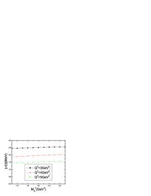
Figure 1: The $\sigma(t)$ with the Borel parameter $M_{B}^{2}$ for $s_{0}=2.25GeV^{2}$.

In this article, we take the middle point for the Borel parameter, $M_{B}^{2}=2.0GeV^{2}$ in numerical analysis, such a specialization will not lead to much uncertainties on the final results and impair the predictive ability.

There are two independent interpolating currents with spin $\frac{1}{2}$ and isospin $\frac{1}{2}$, both are expected to excite the ground state proton from the vacuum, the general form of the proton current can be written as [37]

$$J(x,t) = \epsilon^{abc}\left\{\left[u_{a}^{T}(x)C\gamma_{5}d_{b}(x)\right]u_{c}(x)+t\left[u_{a}^{T}(x)Cd_{b}(x)\right]\gamma_{5}u_{c}(x)\right\},$$ (13)

in the limit $t=-1$, we recover the Ioffe current. The Monte-Carlo calculations for the two-point vacuum correlation function indicate that the optimal mixing be $t=-1.2$, the threshold parameter be $\sqrt{s_{0}}=(1.53\pm 0.41)GeV$ and the mass of the proton be $M=(1.17\pm 0.26)GeV$ [38], furthermore, the Monte-Carlo method has been successfully applied in studying the axial coupling constant and the magnetic moments of the decuplet baryons [39]. Here we take the Ioffe-type current $\eta(x)$ in Eq.(3) to keep in consistent with the sum rules used in determining the parameters in the light-cone distribution amplitudes, $\phi_{3}^{0}$, $\phi_{6}^{0}$, $\phi_{4}^{0}$, $\phi_{5}^{0}$, $\xi_{4}^{0}$, $\xi_{5}^{0}$, $\psi_{4}^{0}$, $\psi_{5}^{0}$, $\phi_{3}^{-}$, $\phi_{3}^{+}$, $\phi_{4}^{-}$, $\phi_{4}^{+}$, $\psi_{4}^{-}$, $\psi_{4}^{+}$, $\xi_{4}^{-}$, $\xi_{4}^{+}$, $\phi_{5}^{-}$, $\phi_{5}^{+}$, $\psi_{5}^{-}$, $\psi_{5}^{+}$, $\xi_{5}^{-}$, $\xi_{5}^{+}$, $\phi_{6}^{-}$, $\phi_{6}^{+}$; furthermore, we take the physical mass for the proton rather than determine it from the corresponding sum rules, this obviously leads to some deviations from the Monte-Carlo adjusted threshold parameter $s_{0}$.

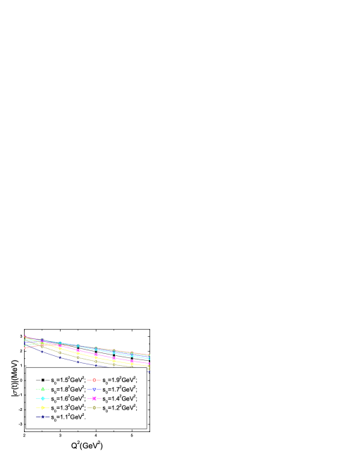
Figure 2: The $\sigma(t)$ with the central values of the input parameters.

In the Fig.2, we plot the dependence on the threshold parameter $s_{0}$ for the sum rules in a large range, $\sqrt{s_{0}}=(1.5\pm 0.4)GeV$. From the figure, we can see that in the region $Q^{2}>3GeV^{2}$, the scalar form-factor is insensitive to threshold parameter $s_{0}$, while in the region $Q^{2}<3GeV^{2}$, the curves for the form-factor $\sigma(t=-Q^{2})$ with $\sqrt{s_{0}}<1.5GeV$ are quite different from those ones with $\sqrt{s_{0}}>1.5GeV$, which may be due to the contributions from the high resonances and continuum states. For simplicity, we choose the standard value for the threshold parameter $s_{0}$, $s_{0}=2.25GeV^{2}$ to subtract the contributions from the higher resonances and continuum states, i.e. we restrict the range of integral to the energy region below the Roper resonance ($N(1440)$); on the other hand, it is large enough to include all the contributions from the proton. The current masses for the $u$ and $d$ quarks are, $m_{u}=(1.5-4)MeV$ and $m_{d}=(4-8)MeV$ from the Particle Data Group in 2004 [35], we choose $\hat{m}=\frac{m_{u}+m_{d}}{2}=5MeV$. For $Q^{2}=(2-5)GeV^{2}$, $x\geq x_{0}=0.5-0.7$, and the average value $\langle x\rangle=0.75-0.85$, with the intermediate and large space-like momentum $Q^{2}$, the end-point contributions (or the Feynman mechanism) are dominant , it is consistent with the growing consensus that the onset of the perturbative QCD region in exclusive processes is postponed to very large energy scales.

The parameters in the light-cone distribution amplitudes $\phi_{3}^{0}$, $\phi_{6}^{0}$, $\phi_{4}^{0}$, $\phi_{5}^{0}$, $\xi_{4}^{0}$, $\xi_{5}^{0}$, $\psi_{4}^{0}$, $\psi_{5}^{0}$, $\phi_{3}^{-}$, $\phi_{3}^{+}$, $\phi_{4}^{-}$, $\phi_{4}^{+}$, $\psi_{4}^{-}$, $\psi_{4}^{+}$, $\xi_{4}^{-}$, $\xi_{4}^{+}$, $\phi_{5}^{-}$, $\phi_{5}^{+}$, $\psi_{5}^{-}$, $\psi_{5}^{+}$, $\xi_{5}^{-}$ ,$\xi_{5}^{+}$, $\phi_{6}^{-}$, $\phi_{6}^{+}$ are scale dependent and can be calculated with the corresponding QCD sum rules, the approximated central values are presented in the Table 1.

	$\phi_{i}^{0}$	$\phi_{i}^{-}$	$\phi_{i}^{+}$	$\psi_{i}^{0}$	$\psi_{i}^{-}$	$\psi_{i}^{+}$	$\xi_{i}^{0}$	$\xi_{i}^{-}$	$\xi_{i}^{+}$
twist-3: $i=3$	$\phantom{-}0.53$	$\phantom{-}2.11$	0.57
twist-4: $i=4$	$-1.08$	$\phantom{-}3.22$	2.12	1.61	$-6.13$	0.99	0.85	$\phantom{-}2.79$	0.56
twist-5: $i=5$	$-1.08$	$-2.01$	1.42	1.61	$-0.98$	-0.99	0.85	$-0.95$	0.46
twist-6: $i=6$	$\phantom{-}0.53$	$\phantom{-}3.09$	-0.25

Table 1: Numerical values for the parameters, the values are given in units of $10^{-2}\,{\rm GeV^{2}}$ [29].

They are functions of eight independent parameters, $f_{N}$, $\lambda_{1}$, $\lambda_{2}$, $V_{1}^{d}$, $A_{1}^{u}$, $f_{d}^{1}$, $f_{d}^{2}$ and $f_{u}^{1}$, the explicit expressions are presented in the appendix, for detailed and systematic studies about this subject, one can consult Ref.[29]. Here we neglect the scale dependence and take the following values for the eight independent parameters, $f_{N}=(5.3\pm 0.5)\times 10^{-3}GeV^{2}$, $\lambda_{1}=-(2.7\pm 0.9)\times 10^{-2}GeV^{2}$, $\lambda_{2}=(5.1\pm 1.9)\times 10^{-2}GeV^{2}$, $V_{1}^{d}=0.23\pm 0.03$, $A_{1}^{u}=0.38\pm 0.15$, $f_{1}^{d}=0.6\pm 0.2$, $f_{2}^{d}=0.15\pm 0.06$, $f_{1}^{u}=0.22\pm 0.15$. In estimating those parameters with the QCD sum rules, only the first few moments are taken into account, the values are not very accurate. One can map the uncertainties of the input parameters into the uncertainties of the adjusted phenomenological parameters [38, 39], for example, the threshold parameter $s_{0}$, the mass of the proton $M$, the scalar form-factor $\sigma(t=-Q^{2})$, etc, with the Monte-Carlo method through $\chi^{2}$ minimization, which may be the most realistic estimates of the uncertainties as there are many input parameters which can be taken into account simultaneously, however, we are no expert in Monte-Carlo simulation, the traditional uncertainties analysis is chosen in this article.

We perform the operator product expansion in the light-cone with large $Q^{2}$ and $P^{\prime 2}$, the scalar form-factor $\sigma(t=-Q^{2})$ make sense at the range $Q^{2}>2GeV^{2}$, with the low momentum transfers, the operator product expansion is questionable. In this article, we devote to calculate the scalar form-factor at the range $Q^{2}>2GeV^{2}$, which corresponding to the size about $0.1fm$, $(q-xP)^{2}\rightarrow xM_{B}^{2}$ after the Borel transformation, in the region $M_{B}^{2}=(1.5-2.5)GeV^{2}$, $\frac{1}{\sqrt{xM_{B}^{2}}}\leq\frac{1}{\sqrt{0.5\times 1.5}GeV}\sim 0.24fm$, retaining only the three valence quark light-cone distribution amplitudes up to twist-6 is reasonable. The size of the proton is about the order of $1fm$ which corresponding to the confinement scale $\Lambda_{QCD}\approx 0.2GeV$, we only investigate short distance physics inside the proton. With smaller momentum transfers, the contributions from the soft (small virtual) gluons and quarks become larger, and the multi-parton configurations become more and more important, the quark and gluons degrees of freedom have to be integrated out, we can work in the hadronic representation and resort to the chiral perturbation theory to deal with the problems [10, 11, 12]. In numerical analysis, we observe that the scalar form-factor $\sigma(t=-Q^{2})$ is sensitive to the four parameters, $\lambda_{1}$, $f^{d}_{1}$, $f^{d}_{2}$ and $f^{u}_{1}$, which are shown in Fig.3, Fig.4, Fig.5 and Fig.6, respectively.

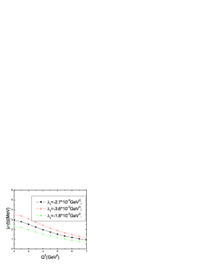
Figure 3: The $\sigma(t)$ with the $Q^{2}$ for the central values of the parameters except $\lambda_{1}$ .

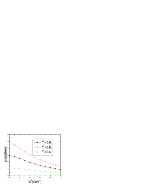
Figure 4: The $\sigma(t)$ with the $Q^{2}$ for the central values of the parameters except $f^{d}_{1}$.

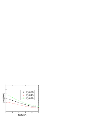
Figure 5: The $\sigma(t)$ with the $Q^{2}$ for the central values of the parameters except $f^{d}_{2}$.

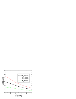
Figure 6: The $\sigma(t)$ with the $Q^{2}$ for the central values of the parameters except $f^{u}_{1}$.

Small variations of those parameters can lead to large changes for the values, the large uncertainties can impair the predictive ability of the sum rules, and those parameters $\lambda_{1}$, $f^{d}_{1}$, $f^{d}_{2}$ and $f^{u}_{1}$ should be refined to make robust predications. The final numerical values for the scalar form-factor $\sigma(t=-Q^{2})$ at the intermediate and large space-like momentum regions $Q^{2}>2GeV^{2}$ are plotted in the Fig.7, from the figure, we can see that the values of the scalar form-factor $\sigma(t=-Q^{2})$ are compatible with the calculations of lattice QCD [13] and chiral quark models [36]. If we take the values from the recent analysis of the $\pi N$ scattering data, $\sigma(0)\approx(\Sigma_{\pi N}=79\pm 7MeV)$, as input, the results from the lattice calculation give $\sigma(-2GeV^{2})<\sigma(0)\times 0.1\approx 7.9MeV$, our results $|\sigma(-2GeV^{2})|\approx(2.9\pm 2.7)MeV$ are smaller, however, reasonable. The $\alpha_{s}$ corrections to the scalar form-factor of the proton may be significant, quantitative conclusion can be reached after the solid calculations, the calculations are tedious though not impossible, and beyond the present work. In the case of the $\pi$ meson, the $\alpha_{s}$ corrections of the twist-2 light-cone distribution amplitude reproduce the $\frac{1}{Q^{2}}$ behavior for the electro-magnetic form-factor with large $Q^{2}$, which corresponding to the hard re-scattering mechanism [24]. The contributions from the four-particle (and five-particle) nucleon distribution amplitudes with a gluon or quark-antiquark pair in addition to the three valence quarks are usually not expected to play any significant roles [32] and neglected here. The consistent and complete LCSR analysis should include the contributions from the perturbative $\alpha_{s}$ corrections, the distribution amplitudes with additional valence gluons and quark-antiquark pairs, and improve the parameters which enter in the LCSRs.

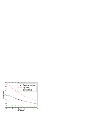
Figure 7: The $\sigma(t)$ with the $Q^{2}$.

4 Conclusion

In this work, we calculate the scalar form-factor $\sigma(t=-Q^{2})$ of the proton in the framework of the LCSR approach up to twist-6 three valence quark light-cone distribution amplitudes and observe the scalar form-factor $\sigma(t=-Q^{2})$ with intermediate and large momentum transfers, $Q^{2}>2GeV^{2}$, has significant contributions from the end-point (or soft) terms, it is consistent with the growing consensus that the onset of the perturbative QCD region in exclusive processes is postponed to very large energy scales. In numerical analysis, we observe that the scalar form-factor $\sigma(t=-Q^{2})$ is sensitive to the four parameters, $\lambda_{1}$, $f^{d}_{1}$, $f^{d}_{2}$ and $f^{u}_{1}$, small variations of those parameters can lead to large changes for the values. The large uncertainties can impair the predictive ability of the sum rules, the parameters $\lambda_{1}$, $f^{d}_{1}$, $f^{d}_{2}$ and $f^{u}_{1}$ should be refined to make robust predications. The numerical values for the $\sigma(t=-Q^{2})$ are compatible with the calculations from the chiral quark model and lattice QCD. The consistent and complete LCSR analysis should include the contributions from the perturbative $\alpha_{s}$ corrections, the distribution amplitudes with additional valence gluons and quark-antiquark pairs, and improve the parameters which enter in the LCSRs.

Appendix

$$\phi_{3}^{0}=\phi_{6}^{0}=f_{N}\,,\hskip 8.5359pt \phi_{4}^{0}=\phi_{5}^{0}=\frac{1}{2}\left(\lambda_{1}+f_{N}\right)\,,$$

$$\xi_{4}^{0}=\xi_{5}^{0}=\frac{1}{6}\lambda_{2}\,, \psi_{4}^{0}=\psi_{5}^{0}=\frac{1}{2}\left(f_{N}-\lambda_{1}\right)\,.$$

$$\tilde{\phi}_{3}^{-} = \frac{21}{2}A_{1}^{u},$$

$$\tilde{\phi}_{3}^{+} = \frac{7}{2}(1-3V_{1}^{d}),$$

$$\phi_{4}^{-} = \frac{5}{4}\left(\lambda_{1}(1-2f_{1}^{d}-4f_{1}^{u})+f_{N}(2A_{1}^{u}-1)\right)\,,$$

$$\phi_{4}^{+} = \frac{1}{4}\left(\lambda_{1}(3-10f_{1}^{d})-f_{N}(10V_{1}^{d}-3)\right)\,,$$

$$\psi_{4}^{-} = -\frac{5}{4}\left(\lambda_{1}(2-7f_{1}^{d}+f_{1}^{u})+f_{N}(A_{1}^{u}+3V_{1}^{d}-2)\right)\,,$$

$$\psi_{4}^{+} = -\frac{1}{4}\left(\lambda_{1}(-2+5f_{1}^{d}+5f_{1}^{u})+f_{N}(2+5A_{1}^{u}-5V_{1}^{d})\right)\,,$$

$$\xi_{4}^{-} = \frac{5}{16}\lambda_{2}(4-15f_{2}^{d})\,,$$

$$\xi_{4}^{+} = \frac{1}{16}\lambda_{2}(4-15f_{2}^{d})\,,$$

$$\phi_{5}^{-} = \frac{5}{3}\left(\lambda_{1}(f_{1}^{d}-f_{1}^{u})+f_{N}(2A_{1}^{u}-1)\right)\,,$$

$$\phi_{5}^{+} = -\frac{5}{6}\left(\lambda_{1}(4f_{1}^{d}-1)+f_{N}(3+4V_{1}^{d})\right)\,,$$

$$\psi_{5}^{-} = \frac{5}{3}\left(\lambda_{1}(f_{1}^{d}-f_{1}^{u})+f_{N}(2-A_{1}^{u}-3V_{1}^{d})\right)\,,$$

$$\psi_{5}^{+} = -\frac{5}{6}\left(\lambda_{1}(-1+2f_{1}^{d}+2f_{1}^{u})+f_{N}(5+2A_{1}^{u}-2V_{1}^{d})\right)\,,$$

$$\xi_{5}^{-} = -\frac{5}{4}\lambda_{2}f_{2}^{d}\,,$$

$$\xi_{5}^{+} = \frac{5}{36}\lambda_{2}(2-9f_{2}^{d})\,,$$

$$\phi_{6}^{-} = \phantom{-}\frac{1}{2}\left(\lambda_{1}(1-4f_{1}^{d}-2f_{1}^{u})+f_{N}(1+4A_{1}^{u})\right)\,,$$

$$\phi_{6}^{+} = -\frac{1}{2}\left(\lambda_{1}(1-2f_{1}^{d})+f_{N}(4V_{1}^{d}-1)\right)\,.$$

References

[1] E. Reya, Rev. Mod. Phys. 46 (1974) 545 ; R. L. Jaffe, Phys. Rev. D21 (1980)
3215.
[2] T. P. Cheng, Phys. Rev. D38 (1988) 2869 .
[3] A. Bottino, F. Donato, N. Fornengo and S. Scopel,
Astropart. Phys. 13 (2000) 215 .
[4] U. Chattopadhyay, A. Corsetti and P. Nath,
Phys. Rev. D66 (2002) 035003.
[5] G. Prezeau, A. Kurylov, M. Kamionkowski and P. Vogel,
Phys. Rev. Lett. 91 (2003) 231301.
[6] T. P. Cheng and R. Dashen, Phys. Rev. Lett. 26 (1971) 594.
[7]
R. Koch, Z. Phys. C 15 (1982) 161 .
[8]
J. Gasser, H. Leutwyler and M. E. Sainio, Phys. Lett. B253 (1991) 252; Phys. Lett. B253 (1991) 260.
[9] M. M. Pavan, I. I. Strakovsky, R. L. Workman, R. A.
Arndt, PiN Newslett. 16 (2002) 110; M. E. Sainio, PiN
Newslett. 16 (2002) 138.
[10] V. Bernard, N. Kaiser and U. G. Meissner, Z. Phys.
C 60 (1993) 111 ; ibid, Phys. Lett. B389 (1996)
144 .
[11] B. Borasoy and U. G. Meissner, Phys. Lett.
B365 (1996) 285 ; B. Borasoy, and U. G. Meissner, Ann. Phys.
(N.Y.) 254 (1997) 192; B. Borasoy, Eur. Phys. J. C8
(1999) 121.
[12] Y. Oh, W. Weise, Eur. Phys. J. A4 (1999) 363 .
[13] S.J. Dong, J. F. Lagae, K. F. Liu, Phys. Rev. D 54 (1996)
5496 .
[14] S. Güsken, P. Ueberholz, J. Viehoff, N. Eicker,
P. Lacock, T. Lippert, K. Schilling, A. Spitz, T. Struckmann, Phys.
Rev. D59 (1999) 054504 .
[15] D. B. Leinweber, A. W. Thomas, S. V. Wright,
Phys. Lett. B482 (2000) 109 ; D. B. Leinweber, A. W. Thomas,
R. D. Young, Phys. Rev. Lett. 92 (2004) 242002;
D. B. Leinweber, A. W. Thomas, K. Tsushima, and
S. V. Wright, Phys. Rev. D61 (2000) 074502.
[16] M. Procura, T. R. Hemmert, W. Weise, Phys. Rev.
D69 (2004) 034505 .
[17] J.-P. Blaizot, M. Rho, N. N. Scoccola, Phys. Lett.
B209 (1988) 27.
[18] D. Diakonov, V. Yu. Petrov, M. Praszaĺowicz,
Nucl. Phys. B323 (1989) 53.
[19] V. E. Lyubovitskij, T. Gutsche, A. Faessler,
E. G. Drukarev, Phys. Rev. D63 (2001) 054026.
[20] P. Schweitzer, Phys. Rev. D69 (2004) 034003;
P. Schweitzer, Eur. Phys. J. A22 (2004) 89.
[21] V. V. Flambaum, A. Hoell, P. Jaikumar, C. D. Roberts, S. V.
Wright, nucl-th/0510075.
[22]
I. I. Balitsky, V. M. Braun and A. V. Kolesnichenko, Nucl. Phys.
B312 (1989) 509; V. L. Chernyak and I. R. Zhitnitsky, Nucl.
Phys. B345 (1990) 137; V. L. Chernyak and A. R. Zhitnitsky,
Phys. Rept. 112 (1984) 173.
[23] M. A. Shifman, A. I. Vainshtein and V. I. Zakharov,
Nucl. Phys. B147 (1979) 385, 448.
[24]
V. Braun and I. Halperin, Phys. Lett. B328 (1994) 457; V. M.
Braun, A. Khodjamirian and M. Maul,
Phys. Rev. D61 (2000) 073004.
[25]
V. M. Braun, hep-ph/9801222; P. Colangelo and A. Khodjamirian,
hep-ph/0010175.
[26] V. M. Braun, A. Lenz, N. Mahnke,
Phys. Rev. D65 (2002) 074011;
A. Lenz, M. Wittmann, E. Stein, Phys. Lett. B581 (2004) 199;
V. M. Braun, A. Lenz, G. Peters, A.V. Radyushkin, hep-ph/0510237 .
[27] M. Q. Huang, D. W. Wang, Phys. Rev. D69 (2004)
094003.
[28]
V. L. Chernyak and I. R. Zhitnitsky, Nucl. Phys. B246 (1984)
52; I. D. King and C. T. Sachrajda, Nucl. Phys. B279 (1987)
785; V. L. Chernyak, A. A. Ogloblin and I. R. Zhitnitsky, Sov. J.
Nucl. Phys. 48 (1988) 536; Z. Phys. C 42 (1989) 583.
[29]
V. Braun, R. J. Fries, N. Mahnke and E. Stein, Nucl. Phys. B
589 (2000) 381; Erratum-ibid. B607 (2001) 433.
[30]
G. P. Lepage and S. J. Brodsky, Phys. Rev. Lett. 43 (1979) 545,
1625 (E); V. A. Avdeenko, V. L. Chernyak and S. A. Korenblit,
Yad. Fiz. 33 (1981) 481;
S. J. Brodsky, G. P. Lepage and A. A. Zaidi,
Phys. Rev. D23 (1981) 1152; S. J. Brodsky and G. P. Lepage,
A. I. Milshtein and V. S. Fadin, Yad. Fiz. 35 (1982) 1603.
[31]
I. I. Balitsky and V. M. Braun, Nucl. Phys. B311 (1989) 541.
[32]
M. Diehl, T. Feldmann, R. Jakob and P. Kroll, Eur. Phys. J. C8 (1999) 409.
[33] B. L. Ioffe and A. V. Smilga Nucl. Phys. B232 (1984) 109 ;
I. I. Balitsky and A. V. Yung, Phys. Lett. B129 (1983) 328.
[34] B. L. Ioffe, Nucl. Phys. B188 (1981) 317; Erratum-ibid. B191 (1981)
591.
[35] Particle Data Group, Phys. Lett. B592 (2004)
1.
[36] H. C. Kim, A. Blotz, C. Schneider, K. Goeke, Nucl. Phys. A596 (1996)
415; T. Inoue, V. E. Lyubovitskij, T. Gutsche, A. Faessler, Phys.
Rev. C69 (2004) 035207.
[37] V. Chung, H. G. Dosch, M. Kremer, D. Scholl,
Nucl. Phys.B197 (1982) 55; H. G. Dosch, M. Jamin and S.
Narison, Phys. Lett.B220 (1989) 251.
[38] D. B. Leinweber, Annals Phys. 254 (1997)
328.
[39] F. X. Lee, Phys. Rev. D57 (1998) 1801; Phys. Lett. B419 (1998)
14; Phys. Rev. C57 (1998) 322; F. X. Lee, D. B. Leinweber, X.
M. Jin, Phys. Rev. D55 (1997) 4066.