Principle of minimum complexity as a new principle in hadronic scattering

Abstract

In this paper a measure of complexity of the system of [$J$ and $\theta$]-quantum states produced in hadronic scattering is introduced in terms of the $[S_{J}(p)$, $S_{\theta}(q)]-$scattering entropies. We presented strong experimental evidence for the saturation of the $[S_{J}^{o1}(p),S_{\theta}^{o1}(q)]-$PMD-SQS optimal limits in the pion-nucleon and kaon-nucleon scatterings. The validity of a principle of minimum complexity in hadronic interaction is supported with high accuracy ($CL>99\%$) by the experimental data on pion-nucleon especially at energies higher than 2 GeV.

1 Introduction

In this paper, by using the optimality [1], the scattering entropies [2-4] $[S_{J}(p)$, $S_{\theta}(q)],$  a measure of the complexity [5] of quantum scattering in terms of Tsallis-like entropies [6] is proposed. Then, the nonextensive statistical behavior, optimality [1] and complexity of the [$J$ and $\theta$]-quantum states in hadronic scatterings are investigated in an unified manner. A connection between optimal states obtained from the principle of minimum distance in the space of quantum states (PMD-SQS)[1] and the most stringent (MaxEnt) entropic bounds on Tsallis-like entropies for quantum scattering is established. A measure of the complexity of quantum scattering in terms of Tsallis-like entropies is proposed. The results on the experimental tests of the PMD-SQS-optimality, as well as on the complexity, obtained by using the experimental pion-nucleon pion-nucleus phase shifts, are presented. Then, the nonextensivity indices p and q are determined from the experimental entropies by a fit with the optimal entropies $[S_{J}^{o1}(p)$, $S_{\theta}^{o1}(q)]$ obtained from the principle of minimum distance in the space of states. In this way strong experimental evidences for the $p-$nonextensivities in the range $0.5\leq p\leq 0.6$ with $q$ correlated via relation $1/p+1/q=2,$ are obtained with high accuracy ($CL>99\%$) from the experimental data of the pion-nucleon and pion-nucleus scatterings.

2 What is the complexity of a quantum system of scattering states?

In the last time many authors have developed and commented on the multiplicity and variety of definitions of complexity (C) in the scientific literature (see Ref.[5] and references therein).

What is the complexity of an interacting system? In general complexity is a concept very difficult to be defined. If we consider that this notion is coming from the original Latin word complexus, which signifies ”entwined”, ”twisted together” then this may interpreted in the following way: in order to have a complex system you need two or more distinct components, which are joined in such a way that it is difficult to separate them. If we look in the Oxford Dictionary we find that something is defined as complex if it is ”made of closely connected parts”. So, in these definitions we find the basic duality between parts which are at the same time distinct and connected. This implies that: a system would be more complex if more parts could be distinguished, and if more connections between them exist. So, the aspects of distinction and connections between the parts of systems determine two dimensions characterizing complexity. Distinction corresponds to the fact that different parts of the complex behaves differently while connections correspond to constrains. Moreover, the distinction leads at the limits to disorder $(\Delta),$ or chaos, while the connection leads to order $(\Omega).$ Complexity can only exist if both aspects are present: neither perfect disorder nor perfect order are complex. Before of a precise mathematical definition of the complexity measure (C) it is useful to point out some intuitive properties of the complexity of the physical systems [5]. These are as follows:

(a) Any reasonable measure of complexity must vanish for the complete ordered or complete disordered states of the system;

(b) Any  complexity must be an universal physical quantity$-$that is, it is applied to any dynamical system;

(c) Any complexity must correspond to mathematical complexity in problem solving.

Current definitions may be divided into three distinct categories according to the following essential feature: (a) Definitions which take complexity as monotonically increasing function of disorder ($\Delta$); (b) Complexity defined as a convex function of disorder ($\Delta$); Complexity defined as monotonically increasing function of order ($\Omega=1-\Delta$).

Since we will express our complexity measure (C) in terms of disorder ($\Delta$), or of order ($\Omega$), we start with the definitions [5]

$$\Delta=\frac{S}{S^{\max}},\vskip 3.0pt plus 1.0pt minus 1.0pt\ \Omega=1-\Delta=1-\frac{S}{S^{\max}}$$ (1)

where S is the Boltzmann-Gibs-Shannon (BGS) entropy

$$S=-\sum p_{i}\ln p_{i}$$ (2)

where p${}_{i},1\leq i\leq N,$ is the probability of i-state of the N states available to the system (the Boltzmann constant k is taken k=1). In the simplest case of an isolated system, the maximum entropy occurs to the equiprobable distribution $p_{i}=1/N,$ $1\leq i\leq N,$ yielding

$$S_{\max}=\ln N$$ (3)

All categories of complexity measures can be included by defining a measure of the form [5]

$$C^{\alpha\beta}(q)=\Delta^{\alpha}\Omega^{\beta}$$ (4)

So, the complexity measures of category I and III correspond to the particular cases: $\alpha>0$, $\beta=0,$and $\alpha=0,\beta>0.$ The category II is obtained when both $\alpha>0$ and $\beta>0.$ Then, the complexity measures $C^{\alpha\beta}(q)$ vanishes at zero disorder and zero order, and has the maximum

$$C_{\max}^{\alpha\beta}=\frac{\alpha^{\alpha}\beta^{\beta}}{(\alpha+\beta)^{(\alpha+\beta)}}\>{\rm at}\>\Delta_{m}=\frac{\alpha}{\alpha+\beta},\>\Omega_{m}=\frac{\beta}{\alpha+\beta}$$ (5)

3  Entropies for two-body scattering

Therefore, in order to introduce a measure of complexity of the hadronic system of quantum states produced in hadronic scatterings we must define the disorder ($\Delta$), or order ($\Omega$) for the hadron-hadron scattering. These physical quantities can be defined just as in Eqs (1)-(2) by using the scattering Boltzman-Gibs-like entropy [2] or more general Tsallis-like scattering entropies introduced by us in Refs. [1,2]. For completeness we start our discussion with $f_{++}(x)$ and $f_{+-}(x)$, $x\in[-1,1]$, as the scattering helicity amplitudes of meson-nucleon scattering

$$M\>(0^{-})+N\>(\frac{1}{2}^{+})\rightarrow M\>(0^{-})+N\>(\frac{1}{2}^{+})$$ (6)

where $x=\cos(\theta),\theta$ being the c.m. scattering angle. The normalization of the helicity amplitudes $f_{++}(x)$ and $f_{+-}(x)$ is chosen such that the c.m. differential cross section $\frac{d\sigma}{d\Omega}(x)$ is given by

$$\frac{d\sigma}{d\Omega}(x)=\mid f_{++}(x)\mid^{2}+\mid f_{+-}(x)\mid^{2}$$ (7)

Since we will work at fixed energy, the dependence of $\sigma_{el}$ and,$\frac{d\sigma}{d\Omega}(x)$ and of $f(x)$, on this variable was suppressed. Hence, the helicities of incoming and outgoing nucleons are denoted by $\mu$, $\mu^{{}^{\prime}}$, and was written as (+),(-), corresponding to $(\frac{1}{2})$ and $(-\frac{1}{2})$, respectively. In terms of the partial waves amplitudes $f_{J+}$ and $f_{J-}$ we have

$$f_{++}(x)=\sum_{J=\frac{1}{2}}^{J_{\max}}(J+1/2)(f_{J-}+f_{J+})d_{\frac{1}{2}\frac{1}{2}}^{J}(x)$$

(8)

where the d${}_{\mu\nu}^{J}(x)$-rotation functions are given by

$$d_{\frac{1}{2}\frac{1}{2}}^{J}(x)=\frac{1}{l+1}\cdot\left[\frac{1+x}{2}\right]^{\frac{1}{2}}\left[\stackrel{{\scriptstyle\circ}}{{P}}_{l+1}(x)-\stackrel{{\scriptstyle\circ}}{{P}}_{l}(x)\right]$$ (9)

$$d_{-\frac{1}{2}\frac{1}{2}}^{J}(x)=\frac{1}{l+1}\cdot\left[\frac{1-x}{2}\right]^{\frac{1}{2}}\left[\stackrel{{\scriptstyle\circ}}{{P}}_{l+1}(x)+\stackrel{{\scriptstyle\circ}}{{P}}_{l}(x)\right]$$ (10)

$P_{l}(x)$ are Legendre Polynomials and prime indicates differentiation with respect to x $\equiv\cos\theta$.

Now, the elastic integrated cross section for the meson-nucleon scattering is expressed in terms of partial amplitudes $f_{J+}$ and $f_{J-}$

$$\sigma_{el}/2\pi=\int_{-1}^{+1}dx\frac{d\sigma}{d\Omega}(x)=\sum_{J=\frac{1}{2}}^{J_{\max}}(2J+1)(\mid f_{J+}\mid^{2}+\mid f_{J-}\mid^{2})$$ (11)

J-nonextensive entropy for the quantum scattering

Now, we define two kind of Tsallis-like scattering entropies. One of them, namely $S_{J}(p),$ p$\in R,$ is special dedicated to the investigation of the nonextensive statistical behavior of the angular momentum $J-$quantum states, and can be defined by

$$S_{J}(p)=\left[1-\sum(2l+1)p_{l}^{p}\right]/(p-1),\vskip 3.0pt plus 1.0pt minus 1.0pt\ \>p\in R,\$$ (12)

where the probability distributions $p_{J},$ is given by

$$p_{J}=\frac{\mid f_{J+}\mid^{2}+\mid f_{J-}\mid^{2}}{\sum_{J=\frac{1}{2}}^{J_{\max}}(2J+1)(\mid f_{J+}\mid^{2}+\mid f_{J-}\mid^{2})},\vskip 3.0pt plus 1.0pt minus 1.0pt\ \sum_{J=\frac{1}{2}}^{J_{\max}}(2J+1)\>p_{J}=1$$ (13)

$\theta$-nonextensive entropy for the quantum scattering

In similar way, for the $\theta-$scattering states considered as statistical canonical ensemble, we can investigate their nonextensive statistical behavior by using an angular Tsallis-like scattering entropy $S_{\theta}(q)$ defined as

$$S_{\theta}(q)=\left[1-\int_{-1}^{+1}dx[P(x)]^{q}\right]/(q-1),\vskip 3.0pt plus 1.0pt minus 1.0pt\ q\in R$$ (14)

where

$$P(x)=\frac{2\pi}{\sigma_{el}}\,\cdot\frac{d\sigma}{d\Omega}(x),\>\int_{-1}^{1}P(x)dx=1$$ (15)

with $\frac{d\sigma}{d\Omega}(x)$ and $\sigma_{el}$ defined by Eqs.(7)-(11).

The above Tsallis-like scattering entropies posses two important properties. First, in the limit $k\rightarrow 1,k\equiv p,q,$ the Boltzman-Gibs kind of entropies is recovered:

$$\lim_{p\rightarrow 1}S_{J}(p)=S_{J}(1)=-\sum(2J+1)p_{J}\ln p_{J}\>$$

(16)

Secondly, these entropies are nonextensive in the sense that

$$S_{A+B}(k)=S_{A}(k)+S_{B}(k)+(1-k)S_{A}(k)S_{B}(k),\vskip 3.0pt plus 1.0pt minus 1.0pt\ k=p,q$$ (17)

for any independent sub-systems $A,B$ $(p_{A+B}=p_{A}\cdot p_{B}).$ Hence, each of the indices $p\neq 1$ or $q\neq 1$ from the definitions (12) and (17) can be interpreted as measuring the degree nonextensivity of the quantum state system.

We next consider the maximum-entropy (MaxEnt) problem

$$\max\{S_{J}(p),S_{\theta}(q)\}{\rm\>when\>}\sigma_{el}={\rm fixed\>and\>}\frac{d\sigma}{d\Omega}(1)={\rm fixed}$$ (18)

as criterion for the determination of the equilibrium distributions $p_{l}^{me}$ and $P^{me}(x)$ for the quantum states from the $(0^{-}\frac{1}{2}\rightarrow 0^{-}\frac{1}{2})-$scattering. For the J-quantum states, in the spin $(0^{-}\frac{1}{2}\rightarrow 0^{-}\frac{1}{2})$ scattering case, these distributions are given by:

$$p_{J}^{me}=p_{J}^{o1}=\frac{1}{2K_{\frac{1}{2}\frac{1}{2}}(1,1)}=\frac{1}{(J_{o}+1)^{2}-1/4},\vskip 3.0pt plus 1.0pt minus 1.0pt\ {\rm\>for}\frac{1}{2}\leq J\leq J_{o},{\rm\>and}$$

(19)

while, for the $\theta-$quantum states, these distributions are as follows

$$P^{me}(x)=P^{o1}(x)=\left[\frac{K_{\frac{1}{2}\frac{1}{2}}^{2}(x,1)}{K_{\frac{1}{2}\frac{1}{2}}(1,1)}\right]$$ (20)

Consequently, by a straightforward calculus we obtain that the solution of the problem (18) is given by

$$S_{J}^{\max}(p)=S_{J}^{o1}(p)=\left[1-[2K_{\frac{1}{2}\frac{1}{2}}(1,1)]^{1-p}\right]/(p-1),{\rm for\>}p>0$$ (21)

$$S_{\theta}^{\max}(q)=S_{\theta}^{o1}(q)=\left[1-\int_{-1}^{+1}dx\left(\frac{\left[K_{\frac{1}{2}\frac{1}{2}}(x,1)\right]^{2}}{K_{\frac{1}{2}\frac{1}{2}}(1,1)}\right)^{q}\right]/(q-1),{\rm\>for\>}q>0$$ (22)

where the reproducing kernel function $K_{\frac{1}{2}\frac{1}{2}}(x,1)$ is given by

$$K_{\frac{1}{2}\frac{1}{2}}(x,1)=\frac{1}{2}\sum_{1/2}^{J_{o}}(2J+1)d_{\frac{1}{2}\frac{1}{2}}^{J}(x)$$ (23)

while the optimal angular momentum $J_{o\>}$ is

$$(J_{o}+1)^{2}-1/4=2K_{\frac{1}{2}\frac{1}{2}}(1,1)=\frac{4\pi}{\sigma_{el}}\frac{d\sigma}{d\Omega}(1)$$ (24)

$d_{\frac{1}{2}\frac{1}{2}}^{J}(x)$ are the usual spin 1/2-rotation functions.

Proof: The proof of the problem (18) is equivalent to the following unconstrained maximization problem:

$$\pounds\rightarrow\max$$ (25)

where the Lagrangian function is defined as

$$\pounds \equiv \lambda_{0}\left\{S_{J}(p),S_{\theta}(q)\right\}+\lambda_{1}\left\{\sigma_{el}/4\pi-\sum(2J+1)\left[\mid f_{J-}\mid^{2}+\mid f_{J+}\mid^{2}\right]\right\}+$$

$$\lambda_{2}\left\{\frac{d\sigma}{d\Omega}(1)-\left[\sum(2J+1){\rm Re}f_{J+}\right]^{2}-\left[\sum(2J+1){\rm Im}f_{J+}\right]^{2}\right\}$$

Hence, the solution of the problem (18), correspond to the the singular case $\lambda_{0}=0,$ and is reduced just to the solution of the minimum constrained distance in space of quantum states:

$$\min\sum(2J+1)\left[\mid f_{J-}\mid^{2}+\mid f_{J+}\mid^{2}\right]{\rm\>when\>}\frac{d\sigma}{d\Omega}(1)={\rm\>is\>\>fixed}$$ (27)

from which we obtain the following analytic form of the optimal scattering helicity amplitudes

$$f_{++}^{o1}(x)=f_{++}(1)\cdot\frac{K_{\frac{1}{2}\frac{1}{2}}(x,1)}{K_{\frac{1}{2}\frac{1}{2}}(1,1)},\>f_{+-}^{o1}(x)=0,$$ (28)

where the reproducing kernels $K_{\frac{1}{2}\frac{1}{2}}(x,1)$ are given by Eqs. (23)-(24). All these results together other are presented in Table 1

4 Complexity measure for quantum scattering  

Now, let us apply the definitions (1) and (4) of the disorder, order, and complexity measure to the nonextensive quantum scattering of the elementary particles. Then, we define the scattering ($J,\theta$)$-$disorders  as follows

$$\Delta_{X}(q)=\frac{S_{X}(q)}{S_{X}^{\max}(q)},\vskip 3.0pt plus 1.0pt minus 1.0pt\ \vskip 3.0pt plus 1.0pt minus 1.0pt\ X\equiv\theta,J$$ (29)

and the corresponding scattering ($\theta,J$)$-$orders by the relations

$$\Omega_{X}(q)=1-\Delta_{X}(q),\vskip 3.0pt plus 1.0pt minus 1.0pt\ \vskip 3.0pt plus 1.0pt minus 1.0pt\ X\equiv\theta,J$$ (30)

where $S_{\theta}(q),S_{J}(q)$ are the scattering Tsallis-like scattering entropies defined in Section 3.

Therefore, using Eqs. (29)-(30) and (12)-(15) we can calculate the scattering complexities $C_{X}^{\alpha\beta}(q)$ defined as follows

$$C_{X}^{\alpha\beta}(q)=\Delta_{X}^{\alpha}(q)\Omega_{X}^{\beta}(q),\vskip 3.0pt plus 1.0pt minus 1.0pt\ X\equiv\theta,J{\>and\>}q\in R$$ (31)

5 Numerical Results

Now, for a systematic experimental investigation of the saturation of the optimality limits in hadron-hadron scattering is necessary to use the formulas from the Table 1 and the available experimental phase-shifts [8-10] to solve the following numerical problems: (i) To reconstruct the experimental pion-nucleon, kaon-nucleon and antikaon-nucleon scattering amplitudes; (ii) To obtain numerical values of the experimental scattering entropies $S_{J}(q),$ $S_{\theta}(q),\overline{S}_{J\theta}(p,q)$ from the reconstructed amplitudes; (iii) To obtain the numerical values of the optimal angular momentum J_o from experimental scattering amplitudes and to calculate the numerical values for the PMD-SQS-optimal entropies $S_{J}^{o1}(q),$ $S_{\theta}^{o1}(q);\overline{S}_{J\theta}(p,q);$ (iv) To obtain numerical values for $\chi_{J}^{2}(p)$ or/and $\chi_{\theta}^{2}(q)$-test functions given by

$$\chi_{X}^{2}(k)=\sum_{i=1}^{n_{\exp}}\left[\frac{[S_{X}(k)]_{i}-[S_{X}^{o1}(k)]_{i}}{[\Delta S_{X}^{o1}]_{i}}\right]^{2},\quad X\equiv J,\theta;\stackrel{{\scriptstyle-}}{{J\theta}}\;\;k\equiv p,q$$ (32)

where

$$\Delta S_{X}^{o1}(k)=|[S_{X}^{o1}(k)]_{J_{o}+1}-[S_{X}^{o1}(k)]_{J_{o}-1}|$$ (33)

are the values of the $PMD-SQS-$optimal entropies $[S_{X}^{o1}(k)]_{J_{o}\pm 1}$ calculated with the optimal angular momenta $J_{o}\pm 1,$ respectively. This procedure is equivalent with assumption of an error of $\Delta J_{o}=\pm 1$ in estimation of the experimental values of the optimal angular momentum $J_{o}.$ The results obtained in this way are presented in the Figs. 1 and Tables 2-4. So, the best fit is obtained (see Tables 2) for the correlated pairs $p$ and $q=p/(2p-1)$ with the values of $p$ in the range $p=$ $0.6$ and $q=p/(2p-1)=3$.0. However, at this level of error analysis the case of the extensive system (p=q=1) of quantum scattering states is also consistent with the experimental data while the pair of nonextensivities (p=3.0,q=0.6) rejected by the values of $\chi^{2}/n_{D}-$test function (see Table 4).

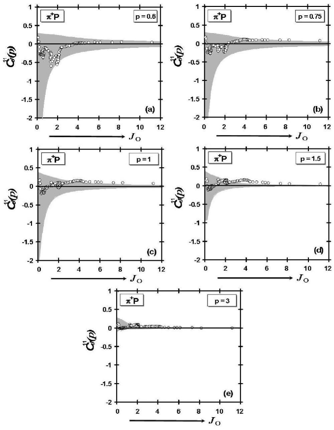
Figure 2: The experimental values of the complexities $C_{J}^{11}(p)$ for $\pi^{+}p-$scatterings, obtained, by using Eqs. (29)-(31), from the available experimental phase-shifts [8-10], are compared with the PMD-SQS-optimal state complexity (full curve $C_{J}^{11}(p)=0).$ The error-band (the grey region) around the optimality curve is calculated by assuming an error of $\Delta J=\pm 1$ in calculation of the optimal angular momentum J_o.

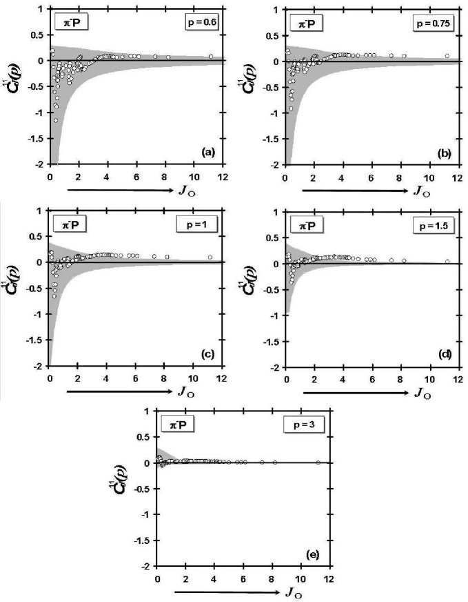
Figure 3: The experimental values of the complexities $C_{J}^{11}(p)$ for $\pi^{-}p-$scatterings, obtained from the available experimental phase-shifts [8], are compared with the PMD-SQS-optimal state complexity (the full curve $C_{J}^{11}(p)=0).$ The error-band (the grey region) around the optimality curve is calculated by assuming an error of $\Delta J=\pm 1$ in calculation of the optimal angular momentum J_o.

Moreover, in Fig. 2-3 we presented the numerical results for the complexity of the J-quantum systems of states produced in the pion-nucleon scattering. So, the experimental values of the complexities $C_{J}^{11}(p)$ for $\pi^{+}p$ and $\pi^{-}p-$scatterings, obtained from the available experimental phase-shifts [19], are compared with the PMD-SQS-optimal state predictions (full curve [$C_{J}^{11}(p)]^{o1}=0$). In all cases, the error-bands (the grey regions) around the optimality curves are calculated by assuming an error of $\Delta J_{o}=\pm 1$ in calculation of the optimal angular momentum J_o From the results of the Figs.2-3 we conclude that the scattering complexities $C_{J}^{11}(p)$ are in excellent agreement with the optimal complexities [$C_{J}^{11}(p)]^{o1}=0$. So, a principle of minimum complexity in hadronic interaction is suggested with high accuracy ($CL>99\%$) by the experimental pion-nucleon scattering data.

6 Summary and Conclusions

In this paper, by using the optimality [1-4] and $[S_{J}(p)$, $S_{\theta}(q)]$-Tsallis-like entropies , the complexity and nonextensivity of the [$J$ and $\theta$]-quantum states produced in hadronic scatterings are investigated. The main results and conclusions can be summarized as follows:

• Using the available experimental phase shifts analysis we calculated the numerical values for the [$S_{J}(p)$, $S_{\theta}(q))$]-Tsallis-like scattering entropies for the pure isospin $I-$scattering states: [$(\pi N)_{I=1/2,3/2}$; $(KN)_{I=0,1}$; $(\overline{K}N)_{I=0,1}$];

• We presented strong experimental evidence for the saturation of the $[S_{J}^{o1}(p),S_{\theta}^{o1}(q)]-$PMD-SQS optimal limits for all nonextensive ($J$, $\theta$)-statistical ensembles of quantum states produced in hadron-hadron scattering (see Fig.1 and Table 2). These results allow to conclude that the $[J]$-quantum system and $[\theta]$-quantum system are produced at ”equilibrium” but with the $[\frac{1}{2p}+\frac{1}{2q}]-$ conjugated nonextensivities $p=0.6$ and $q=p/(2p-1)=3$ in all investigated isospin scattering states: [$(\pi N)_{I=1/2,3/2};(KN)_{I=0,1};(\overline{K}N)_{I=0,1}]$. So the ”geometric origin” of the nonextensivities p and q (as dimensions of the Hilbert spaces $L_{2p}$ and $L_{2q})$ as well as their correlations are experimentally confirmed with high accuracy ($CL>99\%$). The strong experimental evidence obtained here for the nonextensive statistical behavior of the $(J,\theta)-$ quantum scatterings states in the pion-nucleon, kaon-nucleon and antikaon-nucleon scatterings can be interpreted as an indirect manifestation of the presence of the quarks and gluons as fundamental constituents of the scattering system having the strong-coupling long-range regime required by the Quantum Chromodynamics.

• We presented strong experimental evidence fo the validity of a principle of minimum complexity (PMC) in pion-nucleon scattering. PMC is supported with high accuracy ($CL>99\%$) by all the experimental data especially at energies higher than 2 GeV beyond the resonance region.

Finally, we note that further investigations are needed since this saturation of optimality and complexity limits as well as nonextensive statistical behavior of the quantum scattering, evidentiated here with high accuracy $(CL>99\%)$, can be a signature for a new universal law of the quantum scattering.

TABLE CAPTIONS

• The optimal distributions, reproducing kernels, optimal entropies, entropic bands, for the $(0^{-}1/2^{+}\rightarrow 0^{-}1/2^{+})-$scatterings.

• $\chi^{2}/n_{D}$ obtained from comparisons of the experimental scattering entropies: S${}_{J}(p),$ S${}_{\theta}(q)$ with the optimal entropies: S${}_{J}^{o1}(p),$ S${}_{\theta}^{o1}(q),$respectively, for the pair (p=0.6, q=3.0).

• $\chi^{2}/n_{D}$ obtained from comparisons of the experimental scattering entropies: S${}_{J}(p),$ S${}_{\theta}(q)$ with the optimal entropies: S${}_{J}^{o1}(p),$ S${}_{\theta}^{o1}(q),$ respectively, for the pair (p=1.0, q=1.0).

• $\chi^{2}/n_{D}$ obtained from comparisons of the experimental scattering entropies: S${}_{J}(p),$ S${}_{\theta}(q)$ with the optimal entropies: S${}_{J}^{o1}(p),$ S${}_{\theta}^{o1}(q),$ respectively, for the pair (p=3.0, q=0.6).

FIGURES CAPTIONS

• The experimental values of the Tsallis-like scattering entropies $S_{J}(p)$ (12) for $[(\pi N)_{I=1/2,3/2}$; $(KN)_{I=0,1}$; $(\overline{K}N)_{I=0,1}]-$ scatterings, obtained from the available experimental phase-shifts [8-10], are compared with the PMD-SQS-optimal state predictions $S_{J}^{o1}(p)$ (full curve).The error-band (the grey region) around the optimality curve is calculated by assuming an error of $\Delta J_{o}=\pm 1$ in calculation of the optimal angular momentum J_o.

• The experimental values of the complexities $C_{J}^{11}(p)$ for $\pi^{+}p-$scatterings, obtained, by using Eqs. (29)-(31), from the available experimental phase-shifts [8-10], are compared with the PMD-SQS-optimal state complexity (full curve $C_{J}^{11}(p)=0).$ The error-band (the grey region) around the optimality curve is calculated by assuming an error of $\Delta J=\pm 1$ in calculation of the optimal angular momentum J_o.

• The experimental values of the complexities $C_{J}^{11}(p)$ for $\pi^{-}p-$scatterings, obtained from the available experimental phase-shifts [8], are compared with the PMD-SQS-optimal state complexity (the full curve $C_{J}^{11}(p)=0).$ The error-band (the grey region) around the optimality curve is calculated by assuming an error of $\Delta J=\pm 1$ in calculation of the optimal angular momentum J_o.

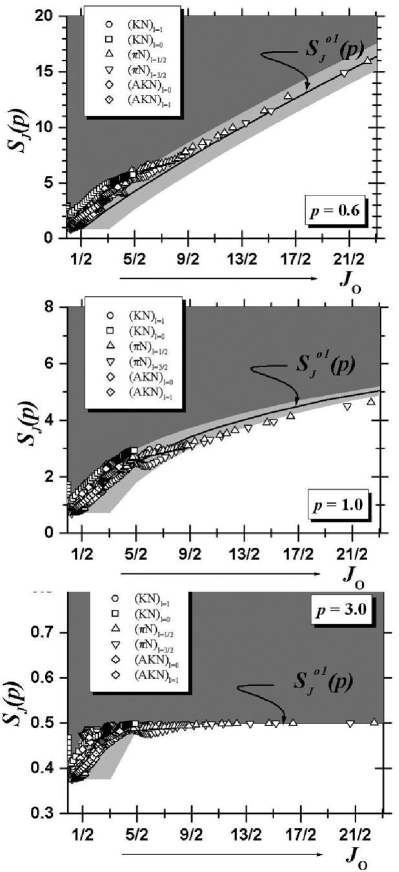
Figure 1: The experimental values of the Tsallis-like scattering entropies $S_{J}(p)$ (12) for $[(\pi N)_{I=1/2,3/2}$; $(KN)_{I=0,1}$; $(\overline{K}N)_{I=0,1}]-$ scatterings, obtained from the available experimental phase-shifts [8-10], are compared with the PMD-SQS-optimal state predictions $S_{J}^{o1}(p)$ (full curve).The error-band (the grey region) around the optimality curve is calculated by assuming an error of $\Delta J_{o}=\pm 1$ in calculation of the optimal angular momentum J_o.

References

- [1] D. B. Ion, Phys. Lett. B 376, 282 (1996).
- [2] D. B. Ion and M. L. D. Ion, Phys Rev. Lett. 81 (1998) 5714; M. L. D. Ion and D. B. Ion, Phys Rev. Lett. 83 (1999) 463. D.B. Ion and M.L.D. Ion, Phys. Rev. E 60, 5261(1999); M.L.D. Ion and D.B. Ion, Phys. Lett. B 482,57 (2000); D.B. Ion and M.L.D. Ion, Phys. Lett. B 503, 263 (2001); D.B. Ion and M.L.D. Ion, Phys. Lett. B 519, 63 (2001); D.B. Ion and M.L.D. Ion, in Classical and Quantum Complexity and Nonexten-sive Thermodynamics, eds. P. Grigolini, C. Tsallis and B.J. West, Chaos , Solitons and Fractals 13 (2002) 547; D. B. Ion and M. L. Ion, Physica A340 (2004) 501.
- [3] M.L.D. Ion and D.B. Ion, Phys. Lett. B 474, 395 (2000).
- [4] D. B. Ion, International J. Theor. Phys. 24, 1217 (1985); D. B. Ion, International J. Theor. Phys. 25, 1257 (1986); D. B. Ion, Rev. Rom. Phys. 26, 15 and 25 (1981); D. B. Ion, Rev. Rom. Phys. 36, 251 (1991).
- [5] J. S. Shiner, M. Davidson and Landsberg, Phys. Rev. E 59 (1999) 1459.
- [6] C. Tsallis, J. Stat. Phys. 52, 479 (1988).
- [7] C. Tsallis and E. P. Borges, Nonextensive statistical mecanics-Applications to nuclear and high energy physics, ArXiv: cond-mat/0301521 (2003), to appear in the Proceedings of the X International Workshop on Multiparticle Production Correlations and Fluctuations in QCD (8-15 June 2002, Crete), ed. N. Antoniou (World Scientific, 2003); An updated bibliography on Nonextensive Statistics can be found at the website: http://tsallis.cat.cbpf.br/biblio.htm. For more general nonextensive entropies see: E. P. Borges and I. Roditi in Phys. Lett. A246, 399 (1998).
- [8] G. Höhler, F. Kaiser, R. Koch, and E. Pietarinen, Physics Data, Handbook of Pion-Nucleon Sattering, 1979, Nr.12-1
- [9] R. A. Arndt and L. D. Roper, Phys. Rev. D31, 2230 (1985).
- [10] M. Alston-Garnjost, R.W. Kenney, D.L. Pollard, R.R. Ross, R.D. Tripp, H. Nicholson, M. Ferro-Luzzi, Phys. Rev. D18, 182 (1978)
- [11] L. R. Lopez, L.J. Caufield, A Principle of Minimum Complexity in Evolution, Lecture Notes in Computer Science, 496, 405 (1991).