PITHA 05/21
December 23, 2005

Spectator scattering at NLO in non-leptonic
$B$ decays: Tree amplitudes

M. Beneke and S. Jäger
Institut für Theoretische Physik E, RWTH Aachen
D–52056 Aachen, Germany

We compute the 1-loop ($\alpha_{s}^{2}$) correction to hard spectator scattering in non-leptonic $B$ decay tree amplitudes. This forms part of the NNLO contribution to the QCD factorization formula for hadronic $B$ decays, and introduces a new rescattering phase that corrects the leading-order result for direct CP asymmetries. Among the technical issues, we discuss the cancellation of infrared divergences, and the treatment of evanescent four-quark operators. The infrared finiteness of our result establishes factorization of spectator scattering at the 1-loop order. Depending on the values of hadronic input parameters, the new 1-loop correction may have a significant impact on tree-dominated decays such as $B\to\pi\pi$.

1 Introduction

The majority of observables at the $B$ factories is connected with branching fractions and CP asymmetries of hadronic $B$ decays to two charmless mesons, for which strong-interaction effects are essential. There is some control over these effects, since the decay amplitudes factorize in the heavy-quark limit. In the QCD factorization framework [1] the matrix elements of the effective weak interaction operators take the (schematic) expression

$$\langle M_{1}M_{2}|Q_{i}|B\rangle=F^{BM_{1}}(0)\,\,T^{\mathrm{I}}_{i}*f_{M_{2}}\phi_{M_{2}}+T^{\mathrm{II}}_{i}*f_{B}\phi_{B+}*f_{M_{1}}\phi_{M_{1}}*f_{M_{2}}\phi_{M_{2}}.$$ (1)

The long-distance strong-interaction effects are now confined to a form factor $F^{BM_{1}}(0)$ at $q^{2}=0$, decay constants $f_{M}$, and light-cone distribution amplitudes $\phi_{M}$. The benefit is that information extraneous to two-body $B$ decays is available for these, and that the short-distance kernels $T_{i}^{\rm I,II}$ can be expanded in a perturbation series in the strong coupling $\alpha_{s}$. Both kernels are currently known from [1] at order $\alpha_{s}$. While for $T_{i}^{\rm I}$ this includes a 1-loop correction to “naive factorization”, in case of $T_{i}^{\rm II}$ the order $\alpha_{s}$ contribution is actually the leading term. It originates from the tree-level exchange of a hard-collinear gluon with the spectator-quark in the $B$ meson, as indicated in Figure 2 below. (The class of corrections from fermion-loop insertions into the gluon propagator is also known [2]. In spectator scattering these $n_{f}$-terms are all connected with the hard-collinear scale and make no contribution to the hard 1-loop correction, which we compute here.)

In this paper we shall compute the 1-loop ($\alpha_{s}^{2}$) correction to the spectator-scattering kernel $T_{i}^{\rm II}$ for what is known as the (topological) “tree amplitudes” in two-body decays. There are several motivations for performing this calculation:

• As in any perturbative QCD calculation the 1-loop correction is necessary to eliminate scale ambiguities. In the present case of spectator scattering the characteristic scales are $m_{b}$ and $(m_{b}\Lambda_{\rm QCD})^{1/2}$. The latter being only about $1.5\,\mbox{GeV}$, a 1-loop calculation is necessary to ascertain the validity of a perturbative treatment by showing that the expansion converges. The 1-loop correction to spectator scattering forms part of the next-to-next-to-leading order (NNLO) contribution to the decay amplitudes.

• At order $\alpha_{s}$ the strong interaction phases, and hence direct CP asymmetries, originate entirely from the imaginary part of the kernel $T_{i}^{\rm I}$ in the first term on the right-hand side of (1). The 1-loop correction to $T_{i}^{\rm II}$ introduces a new rescattering mechanism by spectator scattering. Its calculation represents an important, presumably dominant, part of the next-to-leading order (NLO) result for the CP asymmetries. The NLO result will be needed to resolve or understand potential discrepancies of the LO result with experimental data.

The organization of the paper is as follows. In Section 2 we set up the definitions and matching equations for the calculation of the hard-scattering kernel $T_{i}^{\rm II}$, which is then described in Section 3. The expression for the kernel is given at the end of that section. In Section 4 we obtain the tree amplitudes $\alpha_{1,2}(M_{1}M_{2})$ in a convenient representation, where the light-cone distribution amplitudes are integrated in the Gegenbauer expansion. The numerical effect of the new correction on the tree amplitudes and the $B\to\pi\pi$ branching fractions is investigated in Section 5. We conclude in Section 6.

2 Set-up and matching

2.1 Flavour and colour

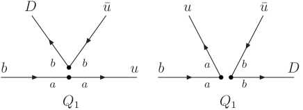
Figure 1: Flavour and colour flow for insertions of $Q_{1}$. The connected fermion lines indicate the contraction of spinor indices. Left: “right insertion”. Right: “wrong insertion”.

We are concerned with the current-current operators in the effective weak Hamiltonian for $b\to u$ transitions given by

$${\cal H}_{\mathrm{eff}} = \frac{G_{F}}{\sqrt{2}}\,V_{uD}^{*}V_{ub}\left(C_{1}Q_{1}+C_{2}Q_{2}\right)+\mathrm{h.c.},$$ (2)

$$Q_{1}=[\bar{u}_{a}\gamma^{\mu}(1-\gamma_{5})b_{a}][\bar{D}_{b}\gamma_{\mu}(1-\gamma_{5})u_{b}],$$

$$Q_{2}=[\bar{u}_{b}\gamma^{\mu}(1-\gamma_{5})b_{a}][\bar{D}_{a}\gamma_{\mu}(1-\gamma_{5})u_{b}],$$

with $a,b$ denoting color, and $D=d$ or $s$. There are two possible flavour flows to the final state as illustrated in Figure 1 for $Q_{1}$. In case of the colour-allowed tree amplitude (left), denoted $\alpha_{1}(M_{1}M_{2})$ following the notation of [3], meson $M_{2}$ represented by the up-going quark lines has the flavour quantum numbers of $[\bar{u}D]$, and $M_{1}$ those of $[\bar{q}_{s}u]$, where $\bar{q}_{s}$ denotes the flavour of the spectator anti-quark in the $\bar{B}$ meson. In case of the colour-suppressed tree amplitude $\alpha_{2}(M_{1}M_{2})$ (right in Figure 1), the corresponding quantum numbers are $[\bar{u}u]$ and $[\bar{q}_{s}D]$, respectively. In addition there exist “penguin contractions”, where the $u$ and $\bar{u}$ fields from $Q_{i}$ are contracted in the same fermion loop. Together with other operators from the effective Hamiltonian they contribute to the (topological) penguin amplitudes, which we do not consider in this paper. Thus, in the computation of the (topological) tree amplitudes there appear four short-distance coefficients, two corresponding to the matrix element of $Q_{1}$ as shown in Figure 1, and two corresponding to $Q_{2}$, which differ only by the colour labels at the operator vertex. It will be seen from the final result that only two of the four coefficients are different, because $Q_{1}$ and $Q_{2}$ are equivalent by a Fierz transformation, when the flavours $u$ and $D$ are not distinguished. However, since we use dimensional regularization, Fierz symmetry cannot be assumed to hold a priori.

We shall refer to the flavour-flow diagrams, where the spinor indices are contracted along the quark lines of $M_{2}$ (left diagram of Figure 1), as the “right insertions” of $Q_{1,2}$; the other contraction (right diagram) is the “wrong insertion”. Exactly the same diagrams contribute to the two right (wrong) insertions, only the colour factor is different for each diagram, since the two operators $Q_{1,2}$ have different colour-orderings. With colour and flavour thus understood, we will omit colour and flavour labels in the subsequent discussion of operator matching.

2.2 Matching onto SCET_I

The short-distance kernels $T^{\rm I,II}_{i}$ can be determined by extracting the hard and hard-collinear momentum regions from quark decay amplitudes according to the strategy of expanding Feynman diagrams by regions [4]. The calculation becomes more transparent, when it is organized as an operator matching calculation in soft-collinear effective theory (SCET) [5]. The spectator-scattering kernel is obtained by the matching sequence QCD $\to$ SCET_I $\to$ SCET_II, by which hard fluctuations ($k\sim m_{b}$, virtuality $m_{b}^{2}$) and hard-collinear fluctuations ($n_{+}k\sim m_{b}$, $k_{\perp}\sim(m_{b}\Lambda_{\rm QCD})^{1/2}$, $n_{-}k\sim\Lambda_{\rm QCD}$, virtuality $m_{b}\Lambda_{\rm QCD}$) are integrated out in two steps. This method has by now been worked out completely for heavy-to-light form factors at large recoil energy of the light meson, both to all orders [6, 7], and by explicit 1-loop calculations of the short-distance coefficients [8, 9, 10]. For application to non-leptonic decays the effective theory has to be extended to include two sets of collinear fields corresponding to the (nearly) light-like directions of the two final-state mesons. As explained in [11] this is a relatively minor complication, because the collinear fields for different directions decouple already at the scale $m_{b}$.

Our SCET conventions follow those of the form-factor calculations [6, 8, 10]. Meson $M_{1}$, which picks up the spectator anti-quark from the $\bar{B}$ meson, moves into the direction of the light-like vector $n_{-}$. The collinear quark field for this direction is denoted by $\xi$ with $n\hskip-4.49997pt/_{-}\xi=0$, the corresponding collinear gluon field is $A_{c1}$. The second meson moves into the opposite direction $n_{+}$, and the collinear fields for this direction are $\chi$, satisfying $n\hskip-4.49997pt/_{+}\chi=0$, and $A_{c2}$. The heavy quark field $h_{v}$ is labeled by the time-like vector $v=(n_{-}+n_{+})/2$ with $v^{2}=1$.

In [6] a power-counting argument has been developed to identify the SCET_I operators that can appear at leading power in the $1/m_{b}$ expansion of heavy-to-light form factors. Applying this argument to the two collinear directions separately, we find that $Q_{1,2}$ can match to only two operators in SCET_I with non-vanishing matrix elements $\langle M_{1}M_{2}|\ldots|\bar{B}\rangle$ for non-singlet mesons $M_{1,2}$. The leading operator in the collinear-2 sector is uniquely given by $(\bar{\chi}W_{c2})(tn_{-})n\hskip-4.49997pt/_{-}(1-\gamma_{5})(W_{c2}^{\dagger}\chi)(0)$. The two operators are then constructed by multiplying this with an A0- and a B1-type current for the $\bar{B}\to M_{1}$ transition [6]. Due to chirality conservation and the requirement that the operator be a Lorentz scalar, there is only one current of each type. The two SCET_I operators thus obtained can be arranged to reproduce the structure of the factorization formula (1) by defining

$$O^{\rm I}(t) = (\bar{\chi}W_{c2})(tn_{-}){\frac{{n\!\!\!/}_{-}}{2}}(1-\gamma_{5})(W_{c2}^{\dagger}\chi)\;\Big{[}\tilde{C}^{(A0)}_{f_{+}}\,({\bar{\xi}}W_{c1}){n\!\!\!/}_{+}(1-\gamma_{5})h_{v}$$

$$\hskip 28.45274pt-\frac{1}{m_{b}}\int d\hat{s}\,\tilde{C}^{(B1)}_{f_{+}}(\hat{s})\,(\bar{\xi}W_{c1}){n\!\!\!/}_{+}[W^{\dagger}_{c1}iD\hskip-5.89996pt/_{\perp c1}W_{c1}](sn_{+})(1+\gamma_{5})h_{v}\Big{]},$$

$${O^{\mathrm{II}}}(t,s) = \frac{1}{m_{b}}\Big{[}(\bar{\chi}W_{c2})(tn_{-}){\frac{{n\!\!\!/}_{-}}{2}}(1-\gamma_{5})(W_{c2}^{\dagger}\chi)\Big{]}$$ (3)

$$\hskip 28.45274pt\times\Big{[}(\bar{\xi}W_{c1}){\frac{{n\!\!\!/}_{+}}{2}}[W^{\dagger}_{c1}iD\hskip-5.89996pt/_{\perp c1}W_{c1}](sn_{+})(1+\gamma_{5})h_{v}\Big{]}.\quad$$

The first operator includes the short-distance coefficients $\tilde{C}^{(A0)}_{f_{+}}$, $\tilde{C}^{(B1)}_{f_{+}}(\hat{s})$ such that its matrix element is proportional to the form factor $f_{+}^{BM_{1}}(0)$ ($A_{0}^{BM_{1}}(0)$ for vector mesons) in QCD (not SCET_I). The expressions for the coefficients to 1-loop (more precisely, their momentum space Fourier transforms) can be found in [10], but they will not be needed here. In (3) fields without position argument are at $x=0$, and the field products within the large brackets are colour-singlets. We do not consider colour-octet operators, since their matrix elements between meson states vanish. Although the second operator carries an apparent $1/m_{b}$ suppression, both operators are in fact leading, because the matrix element of $O^{\rm I}(t)$ is suppressed. Hence, at leading order in $1/m_{b}$, the operators $Q_{1,2}$ from (2) are represented in SCET_I by the equation

$$Q=\int d\hat{t}\,\tilde{T}^{\rm I}(\hat{t})O^{\rm I}(t)+\int d\hat{t}d\hat{s}\,\tilde{H}^{\rm II}(\hat{t},\hat{s}){O^{\mathrm{II}}}(t,s)$$ (4)

with $\hat{s}=n_{+}p^{\prime}s=m_{B}s$, $\hat{t}=n_{-}q\,t=m_{B}t$, and $p^{\prime}$ ($q$) the momentum of $M_{1}$ ($M_{2}$). Of the two matching coefficients $T^{\rm I}(u)=\int d\hat{t}\,e^{iu\hat{t}}\,\tilde{T}^{\rm I}(\hat{t})$ is already known to the 1-loop order ($\alpha_{s}$) [1]. In this paper we compute the 1-loop ($\alpha_{s}^{2}$) correction to

$$H^{\rm II}(u,v)=\int d\hat{t}d\hat{s}\,e^{i(u\hat{t}+(1-v)\hat{s})}\,\tilde{H}^{\rm II}(\hat{t},\hat{s}).$$ (5)

We recall that on accounting for flavour there are actually two copies of ${O^{\mathrm{I}}}(t,s)$, ${O^{\mathrm{II}}}(t,s)$ with different flavour structure, and given the two operators $Q_{1,2}$ in the effective Hamiltonian, there are four different coefficient functions $H^{\rm II}(u,v)$, which we do not distinguish here to simplify the notation.

To see how (1) follows and to make the overall factors explicit, we evaluate the matrix element of (4) for the case that $M_{1}$ and $M_{2}$ are both pseudoscalar mesons. The SCET Lagrangian contains no leading-power interactions between the collinear-2 and collinear-1 fields after decoupling soft gluons from the collinear-2 sector by a field redefinition (second paper of [5]). The matrix elements of ${O^{\mathrm{I}}}(t,s)$, ${O^{\mathrm{II}}}(t,s)$ fall apart into ([10], eqs. (18,81) with $E=n_{+}p^{\prime}/2=m_{B}/2$)

$$\langle M_{2}|(\bar{\chi}W_{c2})(tn_{-}){\frac{{n\!\!\!/}_{-}}{2}}(1-\gamma_{5})(W_{c2}^{\dagger}\chi)|0\rangle=\frac{if_{M_{2}}m_{B}}{2}\int_{0}^{1}du\,e^{iu\hat{t}}\,\phi_{M_{2}}(u),$$

$$\langle M_{1}|(\bar{\xi}W_{c1}){\frac{{n\!\!\!/}_{+}}{2}}[W^{\dagger}_{c1}iD\hskip-5.89996pt/_{\perp c}W_{c1}](sn_{+})(1+\gamma_{5})h_{v}|\bar{B}\rangle=-m_{b}m_{B}\int_{0}^{1}d\tau\,e^{i\tau\hat{s}}\,\Xi_{M_{1}}(\tau),$$ (6)

such that

$$\langle M_{1}M_{2}|Q|\bar{B}\rangle = im_{B}^{2}\,\Bigg{\{}\,f_{+}^{BM_{1}}(0)\int_{0}^{1}du\,T^{\rm I}(u)\,f_{M_{2}}\phi_{M_{2}}(u)$$ (7)

$$\hskip 31.2982pt-\,\frac{1}{2}\int_{0}^{1}dudz\,H^{\rm II}(u,z)\,\Xi_{M_{1}}(1-z)\,f_{M_{2}}\phi_{M_{2}}(u)\Bigg{\}}$$

A demonstration of factorization should provide an argument for the convergence of the various convolution integrals, an issue that is not solved to all orders in perturbation theory for the second term (spectator scattering) in the bracket. The convergence will be explicitly checked at 1-loop in our calculation. At the 1-loop order it is also easy to see by diagrammatic analysis that no operators other than $O^{\rm I}(t)$, $O^{\rm II}(t,s)$ are needed to reproduce the hard momentum regions. In particular any diagrams that match directly onto six-quark operators already in SCET_I are power-suppressed.

2.3 Matching onto SCET_II

To complete the derivation of (1) the hard-collinear scale is integrated out by matching onto SCET_II. Hard-collinear momentum regions appear only in spectator scattering, since an external soft momentum is required. Thus the first term in the bracket of (7) is left unchanged, while the SCET_I form factor $\Xi_{M_{1}}$ related to the matrix element (6) must be matched onto SCET_II. No new calculation is needed for this step, since we can use ([10], eq. (86))

$$\Xi_{M_{1}}(\tau)=\frac{m_{B}}{4m_{b}}\int_{0}^{\infty}d\omega\int_{0}^{1}dv\,J_{\parallel}(\tau;v,\omega)\,\hat{f}_{B}\phi_{B+}(\omega)\,f_{M_{1}}\phi_{M_{1}}(v),$$ (8)

where the “jet function” $J_{\parallel}(\tau;v,\omega)$ has been calculated to 1-loop in [9, 10], and $\hat{f}_{B}$ is $\sqrt{m_{B}}$ times the $B$ decay constant in the static limit ([10], eq. (83)). Inserting this into (7), we obtain

$$\langle M_{1}M_{2}|Q|\bar{B}\rangle = im_{B}^{2}\,\Bigg{\{}\,f_{+}^{BM_{1}}(0)\int_{0}^{1}du\,T^{\rm I}(u)\,f_{M_{2}}\phi_{M_{2}}(u)$$ (9)

$$+\int_{0}^{\infty}d\omega\int_{0}^{1}dudv\,T^{\rm II}(\omega,u,v)\,\hat{f}_{B}\phi_{B+}(\omega)\,f_{M_{1}}\phi_{M_{1}}(v)\,f_{M_{2}}\phi_{M_{2}}(u)\Bigg{\}},$$

which (up to a normalization factor $im_{B}^{2}$) is (1) with

$$T^{\rm II}(\omega,u,v)=-\frac{m_{B}}{8m_{b}}\int_{0}^{1}dz\,H^{\rm II}(u,z)\,J_{\parallel}(1-z;v,\omega).$$ (10)

The jet function is unique, i.e. all four hard-scattering functions $H^{\rm II}(u,z)$ are convoluted with the same $J_{\parallel}(1-z;v,\omega)$.

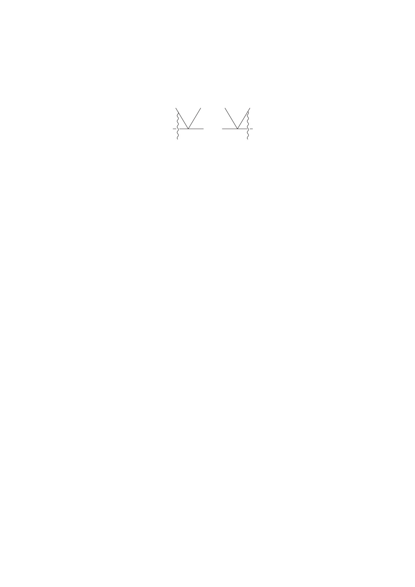
Figure 2: Tree diagrams for $H^{\rm II(0)}(u,z)$.

The tree-level expressions for the hard coefficient functions (when not zero) and the jet function are

$$H^{\rm II(0)}(u,z) = \frac{1}{N_{c}}\,\frac{2}{\bar{u}},$$

$$J_{\parallel}^{(0)}(\bar{z};v,\omega) = -\frac{4\pi\alpha_{s}C_{F}}{N_{c}}\,\frac{1}{m_{B}\omega\bar{v}}\,\delta(\bar{z}-\bar{v}),$$ (11)

where we introduced the QCD colour factors $C_{F}=(N_{c}^{2}-1)/(2N_{c})$, $C_{A}=N_{c}=3$, and the “bar notation”, in which $\bar{x}\equiv 1-x$ for convolution variables $x$. Only the two diagrams shown in Figure 2 have to be computed to obtain $H^{\rm II(0)}(u,z)$. The other two diagrams with attachments to the horizontal quark lines are included in the tree contribution to $T^{\rm I}C_{f_{+}}^{(B1)}$, and thus belong to the $\tilde{T}^{\rm I}O^{\rm I}$ term in (4). Combining the tree coefficients, we obtain

$$T^{\rm II(0)}(\omega,u,v)=\frac{\pi\alpha_{s}C_{F}}{N_{c}^{2}}\,\frac{1}{m_{b}\omega\bar{u}\bar{v}},$$ (12)

which reproduces the result from [1]. Note that $m_{b}$ denotes the $b$-quark pole mass, and $m_{B}$ the $B$ meson mass, but that factors of $m_{b}$ and $m_{B}$ have not been distinguished in [1], since the difference is a power correction.

3 1-loop calculation

In this section we describe technical aspects of the computation of $H^{\rm II}(u,v)$. We calculate the 5-point $b\to q_{c2}\bar{q}_{c2}q_{c1}g_{c1}$ amplitude

$$\langle q(q_{1})\bar{q}(q_{2})q(p^{\prime}_{1})g(p_{2}^{\prime})|Q|b(p)\rangle$$ (13)

and the corresponding SCET_I matrix elements of the right-hand side of (4). With the exception of one class of diagrams to be discussed below, the parton momenta can be restricted to their leading components. Thus for the partons in the collinear-2 direction we put $q_{1}=um_{b}n_{+}/2$, $q_{2}=\bar{u}m_{b}n_{+}/2$, for those in the collinear-1 direction $p_{1}^{\prime}=vm_{b}n_{-}/2$, $p_{2}^{\prime}=\bar{v}m_{b}n_{-}/2$, and for the heavy quark momentum $p^{\mu}=m_{b}v^{\mu}$. For such external momenta the SCET and HQET spinors coincide with the QCD ones.

We use dimensional regularization with $d=4-2\epsilon$ and an anti-commuting $\gamma_{5}$ (NDR scheme). The amplitude (13) has ultraviolet (UV) and infrared (IR) singularities. The former must be subtracted in accordance with the definition of the operators $Q$ in the effective Hamiltonian [13]; the latter in accordance with the definition of the jet function $J_{\parallel}$ and light-cone distribution amplitudes. This is accomplished by using $\overline{\rm MS}$ subtractions and a certain prescription for dealing with evanescent operators. We first discuss the “right insertion” of $Q$, in which the quark spinor indices are contracted according to $[\bar{\chi}\chi][\bar{\xi}h_{v}]$. The “wrong insertion” leads to $[\bar{\xi}\chi][\bar{\chi}h_{v}]$, which differs from the desired order (3) by a Fierz transformation.

3.1 Evanescent operators

The calculation in dimensional regularization is complicated by the presence of evanescent products of Dirac matrices (products that vanish in four dimensions). When such products multiply $1/\epsilon$ poles they need special treatment. In our calculation there are evanescent products that multiply UV singularities. Their definition is related to the renormalization convention for $Q$. The NDR-$\overline{\rm MS}$ scheme corresponds to setting

$$\gamma^{\mu}\gamma^{\nu}\gamma^{\rho}(1-\gamma_{5})\otimes\gamma_{\mu}\gamma_{\nu}\gamma_{\rho}(1-\gamma_{5})=(16-4\epsilon)\,\gamma^{\mu}(1-\gamma_{5})\otimes\gamma_{\mu}(1-\gamma_{5}),$$ (14)

whenever the left-hand side multiplies an UV pole. All other products multiplying UV singularities can be reduced to (14) by permutations.

The evanescent products that multiply IR poles are more complicated. Their treatment is related to the definition of evanescent operators of the $O^{\rm II}(t,s)$ type in SCET_I. To reduce the notation to the essentials, we strip off all the fields from $O^{\rm II}(t,s)$ and represent it only by its Dirac structure,

$$O^{\rm II}(t,s)\to{\frac{{n\!\!\!/}_{-}}{2}}(1-\gamma_{5})\,\otimes\,{\frac{{n\!\!\!/}_{+}}{2}}(1-\gamma_{5})\gamma_{\perp}^{\mu},$$ (15)

where

$$\gamma^{\mu}={\frac{{n\!\!\!/}_{+}}{2}}n^{\mu}_{-}+{\frac{{n\!\!\!/}_{-}}{2}}n^{\mu}_{+}+\gamma^{\mu}_{\perp}.$$ (16)

In our 1-loop calculation we encounter the four operators

$$O_{1} = {\frac{{n\!\!\!/}_{-}}{2}}(1-\gamma_{5})\,\otimes\,{\frac{{n\!\!\!/}_{+}}{2}}(1-\gamma_{5})\gamma_{\perp}^{\mu},$$

$$O_{2} = {\frac{{n\!\!\!/}_{-}}{2}}\gamma_{\perp}^{\mu}\gamma_{\perp}^{\alpha}(1-\gamma_{5})\,\otimes\,{\frac{{n\!\!\!/}_{+}}{2}}(1-\gamma_{5})\gamma_{\perp\alpha},$$

$$O_{3} = {\frac{{n\!\!\!/}_{-}}{2}}\gamma_{\perp}^{\alpha}\gamma_{\perp}^{\beta}(1-\gamma_{5})\,\otimes\,{\frac{{n\!\!\!/}_{+}}{2}}(1-\gamma_{5})\gamma_{\perp}^{\mu}\gamma_{\perp\alpha}\gamma_{\perp\beta},$$

$$O_{4} = {\frac{{n\!\!\!/}_{-}}{2}}\gamma_{\perp}^{\mu}\gamma_{\perp}^{\alpha}\gamma_{\perp}^{\beta}\gamma_{\perp}^{\gamma}(1-\gamma_{5})\,\otimes\,{\frac{{n\!\!\!/}_{+}}{2}}(1-\gamma_{5})\gamma_{\perp\alpha}\gamma_{\perp\beta}\gamma_{\perp\gamma}.$$ (17)

In this notation $O_{1}$ equals $O^{\rm II}(t,s)$. One easily checks that the other three operators are evanescent, i.e. vanish in four dimensions. These operators will disappear from the final result, since we shall renormalize them such that their IR-finite matrix elements vanish, but they must be kept in intermediate steps, hence the matching equation (4) has to be extended to include all four operators on the right-hand side.

Evanescent operators appear already at tree level. In this approximation the matrix element (13) is given by

$$\langle Q_{2}\rangle_{\rm nf}=\frac{1}{N_{c}}\left(\frac{2}{\bar{u}}\langle O_{1}\rangle-\frac{1}{u\bar{u}}\langle O_{2}\rangle\right).$$ (18)

(The “right insertion” of $Q_{1}$ vanishes at tree level, because the colour-trace is zero.) The subscript “nf” (for “non-factorizable”) means that the “factorizable” terms that belong to $T^{\rm I}O^{\rm I}$ are omitted, and only the two diagrams in Figure 2 are included. While one can simply set $\langle O_{2}\rangle=0$ here to recover (11), since no $1/\epsilon$ poles are present at tree level, the appearance of an evanescent operator at tree level implies that one must compute the mixing of $O_{2}$ into $O_{1}$ in the 1-loop calculation.

3.2 UV renormalized 1-loop amplitude

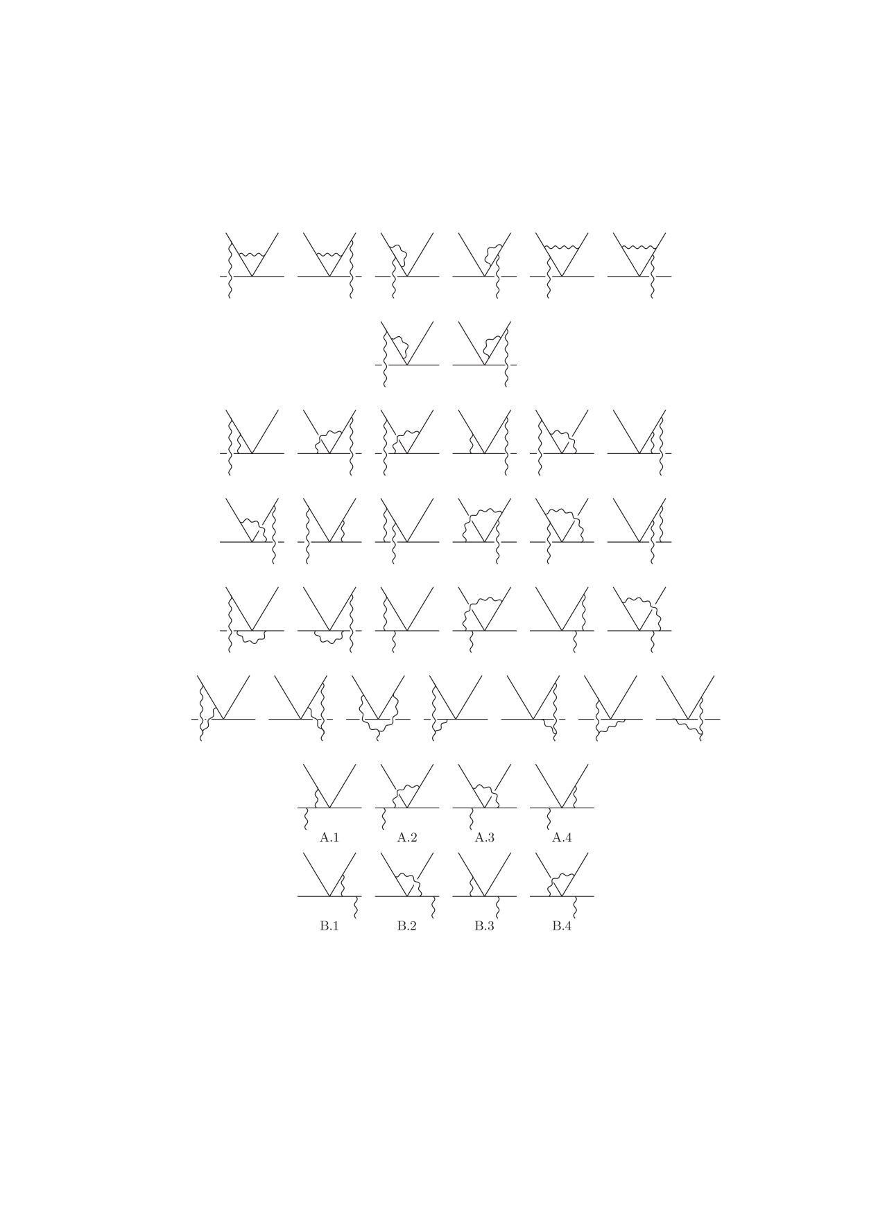
Figure 3: 1-loop diagrams for $\langle Q\rangle_{\rm nf}$.

The calculation of the 1-loop correction to $H^{\rm II}(u,v)$ involves the diagrams shown in Figure 3. The two lines directed upward represent the quark (anti-quark) with collinear-2 momentum proportional to $n_{+}$. The horizontal lines describe an incoming bottom quark, and an outgoing collinear-1 quark with momentum proportional to $n_{-}$. The momentum of the external gluon is also in the $n_{-}$ direction. The calculation of diagrams with no gluon lines that connect the two upper lines to the horizontal lines is not necessary, since the definition of $O^{\rm I}$ is chosen such that these diagrams contribute only to $T^{\rm I}(u)$.

The calculation of the diagrams uses standard methods. The massive box integrals in dimensional regularization can be evaluated adapting the method of [14]. Alternatively, they can be reduced to vertex integrals, because all external momenta are linear combinations of only two vectors $n_{-}$, $n_{+}$. This observation also simplifies the tensor reduction, since one can use

$$k^{\alpha}_{\perp}k^{\beta}_{\perp}\to\frac{1}{d-2}\,g_{\perp}^{\alpha\beta}k_{\perp}^{2}.$$ (19)

The classes A, B of 1-particle reducible diagrams must be included in the amplitude calculation. The heavy-quark propagator to the right of the external gluon line in class A is off-shell by an amount of order $m_{b}^{2}$, hence these diagrams contribute entirely to the short-distance coefficient. Class B is more complicated, since the light-quark propagator with momentum $p^{\prime}=p^{\prime}_{1}+p^{\prime}_{2}$ has small virtuality, hence the diagram is not completely short-distance. The non-local, long-distance contributions cancel in the matching relation against time-ordered products of $O^{\rm I}$ and the SCET interaction Lagrangian as discussed in [8]. The local contribution to the short-distance coefficient can be extracted via the substitution

$$\frac{ip\hskip-4.49997pt/^{\prime}}{{p^{\prime}}^{2}}\to\frac{i}{n_{+}p^{\prime}}\,{\frac{{n\!\!\!/}_{+}}{2}}.$$ (20)

A short-cut to this conclusion is obtained by observing that we can put $p_{1\perp}^{\prime}=p_{2\perp}^{\prime}=p_{\perp}^{\prime}=0$, since we do not match operators with transverse derivatives, and keep only $p^{\prime\mu}=n_{+}p^{\prime}\,n_{-}^{\mu}/2+n_{-}p^{\prime}\,n_{+}^{\mu}/2$. For $p_{\perp}^{\prime}=0$ all relevant interaction terms from the SCET Lagrangian vanish, hence the class B diagrams are purely short-distance. Indeed, since the $n\hskip-4.49997pt/_{-}$ term in the propagator does not contribute owing to the on-shell spinor to the right, the substitution (20) becomes an identity for $p_{\perp}^{\prime}=0$.

Ultraviolet renormalization of the amplitude involves standard counterterms from the QCD Lagrangian as well as the counterterms for $Q$. The UV-renormalized amplitude is written as

$$\langle Q\rangle_{\rm nf}=\sum_{i=1}^{4}\left(A_{i}^{(0)}+A_{i}^{(1)}\right)\langle O_{i}\rangle^{(0)},$$ (21)

where $\langle O_{i}\rangle^{(0)}$ denotes the partonic tree-level matrix element of $O_{i}$, equal to the Dirac matrix products (17) multiplied by the SCET quark spinors and gluon polarization vector. As already mentioned the tree matrix element of the “right insertion” of $Q_{1}$ vanishes due to colour, so $A_{i}^{(0)}=0$ for $Q_{1}$. In this case the 1-loop amplitudes $A_{i}^{(1)}$ are IR-finite and can be evaluated in $d=4$ (after UV renormalization is applied). Hence the evanescent terms $i=2,3,4$ vanish. The “right insertion” of $Q_{2}$ has $A_{i}^{(0)}\not=0$ for $i=1,2$ [see (18)], and the 1-loop amplitudes are IR-divergent. The $i=1,2$ 1-loop terms have a $1/\epsilon^{2}$ singularity, proportional to the tree matrix element, as follows from the universality of soft singularities. $A_{3}^{(1)}$ has a $1/\epsilon$ pole, while $A_{4}^{(1)}$ turns out to be IR-finite. The IR divergences cancel when the QCD amplitude is related to the matching coefficient $H^{\rm II}$ through (4) as explained in the following.

3.3 IR subtractions

We start from the matching equation (4) extended to include the evanescent operators

$$Q=T^{\rm I}\ast O^{\rm I}+\sum_{i}H^{\rm II}_{i}\ast O^{\rm II}_{i}.$$ (22)

Convolutions, which may involve one or two integrations, are now represented by an asterisk. Since we work with matrix elements in states with definite momentum it is convenient to use the momentum-space representation. Expanding all quantities to the 1-loop order, making use of (21) and $O_{i}^{\rm II}=O_{i}$, we obtain

$$\sum_{i}\left(A_{i}^{(1)}+A_{i,\rm f}^{(1)}\right)\langle O_{i}\rangle^{(0)} = T^{{\rm I}(1)}\langle O^{\rm I}\rangle^{(0)}+T^{{\rm I}(0)}\ast\langle O^{\rm I}\rangle^{(1)}$$ (23)

$$+\,\sum_{i}\bigg{(}H^{{\rm II}(1)}_{i}\langle O_{i}\rangle^{(0)}+H^{{\rm II}(0)}_{i}\ast\langle O_{i}\rangle^{(1)}\bigg{)}$$

The factorizable contribution $A_{i,\rm f}^{(1)}$ on the left-hand side comes from 1-loop diagrams with no gluon lines connecting the $\bar{\chi}\chi$ part of the diagram to the $\bar{\xi}A\hskip-4.49997pt/_{\perp c1}h_{v}$ part. It is canceled by the term $T^{{\rm I}(0)}\ast\langle O^{\rm I}\rangle^{(1)}$ on the right-hand side, since the 1-loop matrix element of $O_{i}^{\rm I}$ contains exactly these diagrams in the coefficient function $C_{f_{+}}^{(B1)}$ in its definition (3). The UV-renormalized 1-loop matrix elements of the $O_{i}$ are given by

$$\langle O_{i}\rangle^{(1)}=\sum_{j}\Big{(}M_{ij}^{(1)R}+Z_{ij}^{(1)}\Big{)}\,\langle O_{i}\rangle^{(0)},$$ (24)

where $M_{ij}^{(1)R}$ is the bare matrix element, which depends on the IR regularization scheme $R$, and $Z_{ij}^{(1)}$ the matrix kernel of ultraviolet renormalization factors. When dimensional regularization is used for UV and IR singularities as was done in the calculation of $A_{i}^{(1)}$, the bare matrix elements vanish, since the 1-loop diagrams are scaleless. Hence, inserting (24) into (23), using (3) and $H^{{\rm II}(0)}_{i}=A_{i}^{(0)}$, we obtain

$$A_{1}^{(1)}=H_{1}^{\rm II(1)}+\sum_{i=1}^{2}A_{i}^{(0)}\ast Z_{i1}^{(1)}+(-2)T^{\rm I(1)}C_{f_{+}}^{(B1)(0)}$$ (25)

by comparing the coefficient of $\langle O_{1}\rangle^{(0)}$. We also used that $A_{i}^{(0)}$ is zero for $i=3,4$. The renormalization constants for the evanescent operators are determined by requiring that the IR-finite matrix elements $\langle O_{i}\rangle$ ($i=2,3,4$) vanish [13, 15]. Here “IR-finite” means the matrix element computed with any IR regularization $R=\,$off other than dimensional and with dimensional regularization applied only to the UV singularities. According to (24) this fixes $Z_{21}^{(1)}=-M_{21}^{\rm(1)off}$. Hence the 1-loop short-distance coefficient of the physical (non-evanescent) operator $O^{\rm II}$ is given by

$$H^{\rm II(1)}=A_{1}^{(1)}-A_{1}^{(0)}\ast Z_{11}^{(1)}+A_{2}^{(0)}\ast M_{21}^{\rm(1)off}+2\,T^{\rm I(1)}C_{f_{+}}^{(B1)(0)}.$$ (26)

Note that since the IR-finite matrix elements of the evanescent operators have been made to vanish, only the term $i=1$ survives in (22). It is therefore not necessary to determine the coefficient functions $H^{\rm II}_{i}$ for $i\not=1$. We also note that the renormalization constant $Z_{21}^{(1)}$ is finite, and that $M_{21}^{\rm(1)off}$ is independent of the apparently arbitrary IR regulator. This is because the mixing of an evanescent operator into a physical operator arises through the multiplication of an ultraviolet $1/\epsilon$ pole with a term of order $\epsilon$ from the Dirac algebra, both of which are independent of the IR regularization. The $1/\epsilon^{2}$ poles do not contribute to operator mixing due to their universality.

Eq. (26) provides the final result for the two of the four matching coefficients associated with the right insertions. We briefly discuss the subtraction terms in (26). First note that for the right insertion of $Q_{1}$ the tree amplitudes $A_{i}^{(0)}$ vanish, hence (26) is simply $H^{\rm II(1)}=A_{1}^{(1)}$. This is consistent, since for this case $A_{1}^{(1)}$ is IR-finite as observed above. For the right insertion of $Q_{2}$, all three subtraction terms in (26) are present. Due to factorization in SCET, the renormalization of an operator $[\bar{\chi}\chi]\,[\bar{\xi}A_{\perp c1}h_{v}]$ falls apart into a renormalization factor for the collinear-2 bracket $[\bar{\chi}\chi]$ and one for a B1-type current. $Z_{11}^{(1)}$ is therefore determined by the requirement that the light-cone distribution amplitude of $M_{2}$ and the jet function are defined in the $\overline{\rm MS}$ scheme. This gives $Z_{11}^{(1)}$ as the product of the Brodsky-Lepage kernel [16] and the renormalization kernel $Z_{\parallel}$ for the B1-type current (first paper of [9], [10]). Subtracting $A_{1}^{(0)}\ast Z_{11}^{(1)}$ from $A_{1}^{(1)}$ removes the IR singularities such that $H^{\rm II(1)}$ is finite as must be for a short-distance coefficient. The third term on the right-hand side involves the computation of the 1-loop matrix element of the evanescent operator $O_{2}$. We find that only a single diagram, shown in Figure 4, contributes to $M_{21}^{\rm(1)off}$, such that $M_{21}^{\rm(1)off}$ is proportional to the spin-dependent part of the Brodsky-Lepage kernel. Explicitly,

$$A_{2}^{(0)}\ast M_{21}^{\rm(1)off} = \frac{\alpha_{s}C_{F}}{4\pi}\int_{0}^{1}du^{\prime}\,\frac{(-1)}{N_{c}u^{\prime}\bar{u}^{\prime}}\,(-8)\left(\frac{u^{\prime}}{u}\,\theta(u-u^{\prime})+\frac{\bar{u}^{\prime}}{\bar{u}}\,\theta(u^{\prime}-u)\right)$$ (27)

$$= \frac{\alpha_{s}}{4\pi}\frac{C_{F}}{N_{c}}\,(-8)\left(\frac{\ln u}{\bar{u}}+\frac{\ln\bar{u}}{u}\right)$$

The fourth term $2\,T^{\rm I(1)}C_{f_{+}}^{(B1)(0)}$ follows from $C_{f_{+}}^{(B1)(0)}=-1$ [10] and [1]

$$T^{\rm I(1)}=\frac{\alpha_{s}}{4\pi}\,\frac{C_{F}}{N_{c}}\,V(u)$$ (28)

with $V(u)$ given in (40) below. Note that $H^{\rm II(1)}(u,v)$ is a function of two variables, but like the tree contribution the two subtraction terms (27), (28) depend on $u$, but not on the momentum fraction $v$ related to the collinear-1 momenta.

Figure 4: SCET 1-loop diagram contributing to $M_{21}^{\rm(1)off}$, the mixing of $O_{2}$ into $O_{1}$.

3.4 “Wrong insertion”

The other two matching coefficients are related to the wrong insertions of $Q_{1,2}$ as in the right diagram of Figure 1. We would like to express them as the coefficients of the same SCET_I operator $O^{\rm II}(t,s)$, but the QCD calculation involves Dirac matrix products with a different contraction of spinor indices corresponding to

$$\tilde{O}^{\rm II}(t,s) = \frac{1}{m_{b}}\Big{[}(\bar{\xi}W_{c1})(tn_{-})[W^{\dagger}_{c1}iD\hskip-5.89996pt/_{\perp c1}W_{c1}](sn_{+})(1-\gamma_{5})(W_{c2}^{\dagger}\chi)\Big{]}\,\Big{[}(\bar{\chi}W_{c2})(1+\gamma_{5})h_{v}\Big{]}$$ (29)

$$\to \gamma_{\perp}^{\mu}(1-\gamma_{5})\;{\,\tilde{\otimes}\,}\;(1+\gamma_{5})$$

In the second line we introduced again a short-hand notation that highlights the Dirac structure. The symbol ${\,\tilde{\otimes}\,}$ means that the spinor indices are contracted as in $[\bar{\xi}\chi]\,[\bar{\chi}h_{v}]$. We deal with the required Fierz transformation and evanescent operators simultaneously by introducing the operators

$$\tilde{O}_{0} = {\frac{{n\!\!\!/}_{-}}{2}}(1-\gamma_{5})\,\otimes\,{\frac{{n\!\!\!/}_{+}}{2}}(1-\gamma_{5})\gamma_{\perp}^{\mu},$$

$$\tilde{O}_{1} = \gamma_{\perp}^{\mu}(1-\gamma_{5})\;{\,\tilde{\otimes}\,}\;(1+\gamma_{5}),$$

$$\tilde{O}_{2} = \gamma_{\perp}^{\alpha}(1-\gamma_{5})\;{\,\tilde{\otimes}\,}\;(1+\gamma_{5})\gamma_{\perp}^{\mu}\gamma_{\perp\alpha},$$

$$\tilde{O}_{3} = \gamma_{\perp}^{\mu}\gamma_{\perp}^{\alpha}\gamma_{\perp}^{\beta}(1-\gamma_{5})\;{\,\tilde{\otimes}\,}\;(1+\gamma_{5})\gamma_{\perp\alpha}\gamma_{\perp\beta},$$

$$\tilde{O}_{4} = \gamma_{\perp}^{\alpha}\gamma_{\perp}^{\beta}\gamma_{\perp}^{\gamma}(1-\gamma_{5})\;{\,\tilde{\otimes}\,}\;(1+\gamma_{5})\gamma_{\perp}^{\mu}\gamma_{\perp\alpha}\gamma_{\perp\beta}\gamma_{\perp\gamma}.$$ (30)

Here $\tilde{O}_{0}$ is the short-hand for $O^{\rm II}$. The basis is chosen such that $\tilde{O}_{1}$ and $\tilde{O}_{0}$ are Fierz-equivalent and $\tilde{O}_{2-4}$ vanish in four dimensions. Hence we have one physical operator, $\tilde{O}_{0}$, and four evanescent operators, $\tilde{O}_{1}-\tilde{O}_{0}$, and $\tilde{O}_{2-4}$. The tree matrix element is now given by

$$\langle Q_{1}\rangle_{\rm nf}=\frac{1}{N_{c}}\left(\frac{2}{\bar{u}}\langle\tilde{O}_{1}\rangle+\frac{1}{u}\langle\tilde{O}_{2}\rangle\right),$$ (31)

and the 1-loop amplitude reads

$$\langle Q\rangle_{\rm nf}=\sum_{i=1}^{4}\left(\tilde{A}_{i}^{(0)}+\tilde{A}_{i}^{(1)}\right)\langle\tilde{O}_{i}\rangle^{(0)}.$$ (32)

This does not contain $\langle\tilde{O}_{0}\rangle^{(0)}$, since all diagrams have the “wrong” Fierz-ordering. Proceeding as before and requiring that the infrared-finite matrix elements of the four evanescent operators vanish, we find that (26) is replaced by

$$H^{\rm II(1)}=\tilde{A}_{1}^{(1)}-\tilde{A}_{1}^{(0)}\ast\tilde{Z}_{00}^{(1)}+\tilde{A}_{2}^{(0)}\ast\tilde{M}_{21}^{\rm(1)off}+\tilde{A}_{1}^{(0)}\ast\left(\tilde{M}_{11}^{\rm(1)off}-\tilde{M}_{00}^{\rm(1)off}\right)+2\,T^{\rm I(1)}C_{f_{+}}^{(B1)(0)}$$ (33)

with $\tilde{M}_{21}^{\rm(1)off}$ the bare 1-loop mixing of $\tilde{O}_{2}$ into $\tilde{O}_{1}$, and $\tilde{Z}_{00}^{(1)}=Z_{11}^{(1)}$. The new term $\tilde{A}_{1}^{(0)}\ast(\tilde{M}_{11}^{\rm(1)off}-\tilde{M}_{00}^{\rm(1)off})$ involves the difference of the mixing of $\tilde{O}_{1}$ and $\tilde{O}_{0}$ into themselves. This difference is finite and independent of the IR regulator for the same reason that $\tilde{M}_{21}^{\rm(1)off}$ is. There is one subtle aspect hidden in (33) that requires explanation. As in (23) we would like to cancel the factorizable QCD diagrams against the matrix element of $O^{\rm I}$, but the two terms appear in different Fierz-orderings. The consequence of this is that there should be an extra term related to the factorizable diagrams on the right-hand side of (33). Using that at tree-level only $A_{1,\rm f}^{(0)}$, $\tilde{A}_{1,\rm f}^{(0)}$, $\tilde{A}_{2,\rm f}^{(0)}$ are non-zero, it is given by

$$\tilde{A}_{1,\rm f}^{(1)}-A_{1,\rm f}^{(1)}+\tilde{A}_{2,\rm f}^{(0)}\ast\tilde{M}_{21}^{\rm(1)off}+\tilde{A}_{1,\rm f}^{(0)}\ast\left(\tilde{M}_{11}^{\rm(1)off}-\tilde{M}_{00}^{\rm(1)off}\right).$$ (34)

However, we find that this term vanishes, hence (33) is correct. The subtractions $-\tilde{A}_{1}^{(0)}\ast\tilde{Z}_{00}^{(1)}$ and $2\,T^{\rm I(1)}C_{f_{+}}^{(B1)(0)}$ are identical to the corresponding terms for the right insertion. The other two terms are once again related to an integral over the spin-dependent part of the Brodsky-Lepage kernel. Explicitly, they read

$$\tilde{A}_{2}^{(0)}\ast\tilde{M}_{21}^{\rm(1)off} = \frac{\alpha_{s}}{4\pi}\frac{C_{F}}{N_{c}}\,(-8)\,\frac{\ln u}{\bar{u}},$$

$$\tilde{A}_{1}^{(0)}\ast\left(\tilde{M}_{11}^{\rm(1)off}-\tilde{M}_{00}^{\rm(1)off}\right) = \frac{\alpha_{s}}{4\pi}\frac{C_{F}}{N_{c}}\,(-4)\,\frac{\ln\bar{u}}{u}.\qquad$$ (35)

Despite the different Dirac algebra and subtraction structure we find that the final result for the matching coefficient related to the wrong insertion of $Q_{1}$ ($Q_{2}$) is identical to the one for the right insertion of $Q_{2}$ ($Q_{1}$).

3.5 Matching coefficients

Here we give the final results for the matching coefficients (hard spectator-scattering kernels) $H^{\rm II}(u,v)$ in the convolutions (7), (10). The kernels are independent of the mesons but dependent on their flavour quantum numbers. To make them explicit, we write $\langle[\bar{q}_{s}q_{M_{1}}][\bar{q}_{M_{2}}q_{M_{2}}]|Q|[\bar{q}_{s}b]\rangle$ for $\langle M_{1}M_{2}|Q|\bar{B}\rangle$ to indicate flavour. Then

• for $\langle[\bar{q}_{s}D][\bar{u}u]|Q_{1}|[\bar{q}_{s}b]\rangle$, the contribution of $Q_{1}$ to the colour-suppressed tree amplitude $\alpha_{2}(M_{1}M_{2})$, and for $\langle[\bar{q}_{s}u][\bar{u}D]|Q_{2}|[\bar{q}_{s}b]\rangle$, the contribution of $Q_{2}$ to the colour-allowed tree amplitude $\alpha_{1}(M_{1}M_{2})$, we have

  $$H_{1}^{\rm II}(u,v)=\frac{2}{N_{c}}\left(\frac{1}{\bar{u}}+\frac{\alpha_{s}}{4\pi}\,r_{1}(u,v)\right)$$ (36)

• for $\langle[\bar{q}_{s}u][\bar{u}D]|Q_{1}|[\bar{q}_{s}b]\rangle$, the contribution of $Q_{1}$ to the colour-allowed tree amplitude $\alpha_{1}(M_{1}M_{2})$, and for $\langle[\bar{q}_{s}D][\bar{u}u]|Q_{2}|[\bar{q}_{s}b]\rangle$, the contribution of $Q_{2}$ to the colour-suppressed tree amplitude $\alpha_{2}(M_{1}M_{2})$:

  $$H_{2}^{\rm II}(u,v)=\frac{2}{N_{c}}\,\frac{\alpha_{s}}{4\pi}\,r_{2}(u,v)$$ (37)

Here $r_{1}(u,v)$, $r_{2}(u,v)$ are given by

$$r_{1} = C_{F}\Bigg{[}-\frac{1}{2\bar{u}}\ln^{2}\frac{m_{b}^{2}}{\mu^{2}}+\bigg{(}6-\frac{5}{2\bar{u}}+\frac{2}{\bar{u}}\ln\bar{u}\bigg{)}\ln\frac{m_{b}^{2}}{\mu^{2}}+\frac{u}{\bar{u}}\,\Big{[}V(u)+18\Big{]}$$ (38)

$$\hskip 22.76228pt-\,\frac{2u}{\bar{u}}\,F(v,u)+\frac{2u^{3}}{(\bar{v}-u)^{3}}\,F(v,\bar{u})-\frac{2}{\bar{u}}\Big{(}\ln\bar{u}+\ln\bar{v}\Big{)}i\pi-\frac{1}{\bar{u}}\bigg{(}9+\frac{5}{12}\pi^{2}\bigg{)}$$

$$\hskip 22.76228pt+\,\bigg{(}\frac{u}{\bar{v}-u}-\frac{2u^{2}}{(\bar{v}-u)^{2}}-\frac{2(3u-2)}{\bar{u}}\bigg{)}\Big{[}\log u-i\pi\Big{]}-\frac{2(1-uv)}{u\bar{u}v\bar{v}}\ln(1-uv)$$

$$\hskip 22.76228pt-\,\bigg{(}\frac{u(2-4u+u^{2})}{\bar{u}^{2}(\bar{v}-u)}-\frac{2(2-u)u^{2}}{\bar{u}(\bar{v}-u)^{2}}+\frac{\bar{u}-v+4u\bar{u}v}{u\bar{u}^{2}v^{2}}\bigg{)}\ln(1-\bar{u}v)$$

$$\hskip 22.76228pt+\,\frac{1}{\bar{u}}\big{(}\ln^{2}\bar{u}-\ln^{2}\bar{v}\big{)}+\bigg{(}\frac{u}{\bar{v}-u}-\frac{2u^{2}}{(\bar{v}-u)^{2}}+\frac{\bar{v}+3uv^{2}}{uv^{2}}\bigg{)}\ln\bar{v}$$

$$\hskip 22.76228pt+\,\bigg{(}3+\frac{2}{u\bar{v}}-2\ln v+\Big{(}2+\frac{2}{\bar{u}}\Big{)}\ln\bar{v}\bigg{)}\ln\bar{u}+\bigg{(}3+\frac{2}{\bar{u}}\ln\bar{v}\bigg{)}\ln v$$

$$\hskip 22.76228pt+\,\bigg{(}\frac{1-3u\bar{u}}{\bar{u}^{2}}+\frac{2(3u-2)}{\bar{u}}+2\ln v+\frac{2u}{\bar{u}}\ln\bar{v}\bigg{)}\ln u+\frac{2}{\bar{u}}\,\mathrm{Li}_{2}(\bar{v})\Bigg{]}$$

$$+\left(C_{F}-\frac{C_{A}}{2}\right)\Bigg{[}-\frac{2}{\bar{u}\bar{v}}\,\ln v\,\ln\frac{m_{b}^{2}}{\mu^{2}}+\frac{1}{\bar{u}}\,V(u)+\frac{2u}{v-u}F(v,u)+\frac{2u^{2}}{(\bar{v}-u)^{2}}F(v,\bar{u})$$

$$\hskip 22.76228pt+\,2i\pi\,\bigg{(}\frac{\bar{v}}{\bar{v}-u}+\frac{u}{\bar{u}}\ln\frac{u}{\bar{u}}+\frac{v}{\bar{u}\bar{v}}\ln v+\frac{1}{\bar{u}}\ln\bar{v}\bigg{)}+\frac{1}{\bar{u}}\bigg{[}\ln^{2}\bar{v}+\frac{\pi^{2}}{3}\bigg{]}+\frac{u}{\bar{u}}\big{(}\ln^{2}u-\ln^{2}\bar{u}\big{)}$$

$$\hskip 22.76228pt-\,\frac{1+\bar{v}}{\bar{u}\bar{v}}\ln^{2}v+\bigg{(}\frac{2-3u}{u\bar{u}}+\frac{2}{u\bar{v}}\bigg{)}\ln\bar{u}-\frac{2(1-uv)}{u\bar{u}v\bar{v}}\ln(1-uv)$$

$$\hskip 22.76228pt+\bigg{(}\frac{2(1-3u^{2}+u^{3})}{u\bar{u}v}+\frac{2(1-\bar{v}^{2}\bar{u})}{\bar{u}v\bar{v}}+\frac{2(2-u)u}{v(\bar{v}-u)}\bigg{)}\ln(1-\bar{u}v)$$

$$\hskip 22.76228pt+\,\bigg{(}\frac{1+2u\bar{u}}{\bar{u}^{2}}-\frac{2(1-uv)}{\bar{u}^{2}\bar{v}}+\frac{2u(u\bar{u}-v)}{\bar{u}^{2}(\bar{v}-u)}\bigg{)}\ln u$$

$$\hskip 22.76228pt+\,\bigg{(}\frac{3(1+\bar{v})}{\bar{u}\bar{v}}+\frac{2}{\bar{u}}\ln u-\frac{2}{\bar{u}\bar{v}}\ln\bar{u}\bigg{)}\ln v$$

$$\hskip 22.76228pt-\,\bigg{(}\frac{2-5u-4u^{2}+2u^{3}}{u\bar{u}v}+\frac{(1+2u)\bar{v}}{\bar{u}v}+\frac{2u\bar{u}}{v(\bar{v}-u)}+\frac{2u}{\bar{u}}\ln u$$

$$\qquad\qquad+2\ln\bar{u}+\frac{2(1-2u)}{u\bar{u}\bar{v}}\ln v\bigg{)}\ln\bar{v}$$

$$\hskip 22.76228pt+\,2\,\bigg{\{}\!-\frac{1+2u\bar{v}}{\bar{u}\bar{v}}\,\mathrm{Li}_{2}(u)+\frac{1-u\bar{v}+2u^{2}\bar{v}}{u\bar{u}\bar{v}}\,\mathrm{Li}_{2}(\bar{u})+\frac{1+u\bar{v}}{\bar{u}\bar{v}}\,\mathrm{Li}_{2}(uv)$$

$$\qquad\qquad-\,\frac{1-u\bar{u}\bar{v}}{u\bar{u}\bar{v}}\,\mathrm{Li}_{2}(\bar{u}v)-\frac{1-2u+u\bar{v}}{u\bar{u}\bar{v}}\,\mathrm{Li}_{2}(\bar{v})\bigg{\}}\Bigg{]},$$

$$r_{2} = \frac{1}{2\bar{u}}\,\Big{[}V(u)+2\Big{]}+\frac{u\bar{v}}{\bar{u}(v-u)}\,F(v,u)+\frac{u^{2}\bar{v}}{(\bar{v}-u)^{3}}\,F(v,\bar{u})+\frac{\bar{v}(\bar{v}-3u)}{2(\bar{v}-u)^{2}}\,\Big{[}\ln\bar{v}-i\pi\Big{]}$$ (39)

$$+\,\bigg{(}\frac{1+u^{2}}{2\bar{u}^{2}}+\frac{u}{2\bar{u}^{2}\,\bar{v}}-\frac{u^{2}}{(\bar{v}-u)^{2}}-\frac{u}{2(\bar{v}-u)}\bigg{)}\ln u+\frac{\bar{u}+\bar{v}}{u\bar{u}\bar{v}}\,\ln\bar{u}$$

$$+\,\bigg{(}\frac{3}{2\bar{u}}-\frac{1}{2\bar{u}\bar{v}}+\frac{\ln u}{\bar{u}}-\frac{\ln\bar{u}}{\bar{u}}\bigg{)}\ln v-\bigg{(}\frac{1}{u\bar{u}v}+\frac{1}{u\bar{v}}\bigg{)}\ln(1-uv)$$

$$+\,\bigg{(}\!-\frac{1}{2}-\frac{u}{2\bar{u}^{2}\bar{v}}+\frac{u^{2}(\bar{u}^{2}+v)}{\bar{u}^{2}(\bar{v}-u)^{2}}+\frac{u(2+u^{2})}{2\bar{u}^{2}(\bar{v}-u)}\bigg{)}\ln(1-\bar{u}v),$$

where we defined

$$F(v,w) = 2\,\mathrm{Li}_{2}\bigg{(}\!-\frac{\bar{v}w}{\bar{w}}\bigg{)}+2\,\mathrm{Li}_{2}(w)-\mathrm{Li}_{2}(vw)+\frac{1}{2}\ln^{2}\frac{\bar{w}}{\bar{v}}+i\pi\ln\frac{\bar{w}}{\bar{v}},$$

$$V(u) = 6\ln\frac{m_{b}^{2}}{\mu^{2}}-18+3\,\bigg{(}\frac{1-2u}{\bar{u}}\ln u-i\pi\bigg{)}$$ (40)

$$\quad+\bigg{\{}2\,\mathrm{Li}_{2}(u)-\ln^{2}u+\frac{2\ln\,u}{\bar{u}}-(3+2i\pi)\ln u-(u\leftrightarrow\bar{u})\bigg{\}}.$$

The expressions for $r_{1}$ and $r_{2}$ constitute the main technical results of this paper. In applications the kernels always appear in convolutions. In the following we perform the convolution integrals analytically and obtain a compact representation for the (topological) tree amplitudes.

4 Tree amplitudes with NLO spectator scattering

The complete 1-loop correction to spectator scattering is the convolution of the hard-scattering kernels $H^{\rm II}_{1,2}$ with the jet function

$$J_{\parallel}(\bar{z};v,\omega)=-\frac{4\pi\alpha_{s}C_{F}}{N_{c}}\,\frac{1}{m_{B}\omega\bar{v}}\left[\delta(\bar{z}-\bar{v})+\frac{\alpha_{s}}{4\pi}\,j_{\parallel}(\bar{z};v,\omega)\right].$$ (41)

Inserting this and (36), (37) into (10), and expanding to order $\alpha_{s}^{2}$, we obtain

$$T_{i}^{\rm II}(\omega,u,v) = \frac{\pi\alpha_{s}C_{F}}{N_{c}^{2}}\,\frac{1}{m_{b}\omega\bar{v}}\,\left\{\begin{array}[]{l}\displaystyle\frac{1}{\bar{u}}+\frac{\alpha_{s}}{4\pi}\left[r_{1}(u,v)+\frac{1}{\bar{u}}\int_{0}^{1}dz\,j_{\parallel}(z;v,\omega)\right]\quad(i=1)\\[14.22636pt] \displaystyle\frac{\alpha_{s}}{4\pi}\,r_{2}(u,v)\quad(i=2)\end{array}\right.$$ (44)

(The integral $\int_{0}^{1}dz\,j_{\parallel}(z;v,\omega)$ is given analytically in appendix B.1 of [10].) The spectator-scattering contribution to the tree decay amplitudes $\alpha_{1,2}(M_{1}M_{2})$ in the standard normalization is

$$S_{i}=\frac{\hat{f}_{B}f_{M_{1}}}{f_{+}^{BM_{1}}(0)}\int_{0}^{\infty}d\omega\int_{0}^{1}dudv\,T_{i}^{\rm II}(\omega,u,v)\,\phi_{B+}(\omega)\,\phi_{M_{1}}(v)\,\phi_{M_{2}}(u),$$ (45)

see (9). More precisely, accounting for the Wilson coefficients in the effective weak Hamiltonian (2), we have $\alpha_{1}(M_{1}M_{2})|_{\rm sp}=C_{1}S_{2}+C_{2}S_{1}$, $\alpha_{2}(M_{1}M_{2})|_{\rm sp}=C_{1}S_{1}+C_{2}S_{2}$.

4.1 Expansion of convolutions in Gegenbauer moments

The integration over the spectator quark momentum fraction $\omega$ is simple, because $\omega$ appears only in the jet function, or as the over-all factor $1/\omega$. The dependence on the light-cone distribution amplitude of the $B$ meson is encoded in the inverse moment

$$\frac{1}{\lambda_{B}}\equiv\int_{0}^{\infty}\frac{d\omega}{\omega}\,\phi_{B+}(\omega),$$ (46)

and the logarithmic moments

$$\langle L^{n}\rangle=\lambda_{B}\int\frac{d\omega}{\omega}\phi_{B_{+}}(\omega)\ln^{n}\frac{m_{b}\omega}{\mu^{2}}$$ (47)

up to $n=2$. The light-cone distribution amplitude of a light meson, $\phi_{M}$, is conventionally expanded into the eigenfunctions of the 1-loop renormalization kernel,

$$\phi_{M}(x)\,=\,6x\bar{x}\left[1+\sum\limits_{n=1}^{\infty}a_{n}^{M}C^{(3/2)}_{n}(2x-1)\right]\,,$$ (48)

where $a_{n}^{M}$ and $C^{(3/2)}_{n}$ are the Gegenbauer moments and polynomials, respectively. The integrals over $u$ and $v$ can then be performed, the result being represented as a double expansion in the Gegenbauer moments of $M_{1}$ and $M_{2}$. Often, there appear the quantities

$$\Delta_{M}\equiv\int_{0}^{1}dx\,\frac{\phi_{M}(x)}{3x}=1+\sum_{n=1}^{\infty}(-1)^{n}\,a_{n}^{M},\quad\bar{\Delta}_{M}\equiv\int_{0}^{1}dx\,\frac{\phi_{M}(x)}{3\bar{x}}=1+\sum_{n=1}^{\infty}a_{n}^{M},$$ (49)

We give the final result for the tree amplitude parameters $\alpha_{1,2}(M_{1}M_{2})$ in the notation of [3] [eq. (35)], including the 1-loop vertex correction $V_{i}(M_{2})$ not related to spectator scattering,

$$\alpha_{i}(M_{1}M_{2}) = C_{i}+\frac{C_{i\pm 1}}{N_{c}}+\frac{C_{i\pm 1}}{N_{c}}\,\frac{\alpha_{s}C_{F}}{4\pi}\,V_{i}(M_{2})$$ (50)

$$+\,\frac{\pi\alpha_{s}C_{F}}{N_{c}^{2}}\,\frac{9f_{M_{1}}\hat{f}_{B}}{m_{b}f_{+}^{BM_{1}}(0)\lambda_{B}}\,\Big{[}C_{i\pm 1}\,h_{1}(M_{1}M_{2})+C_{i}\,h_{2}(M_{1}M_{2})\Big{]}.$$

The upper signs apply when $i$ is odd (here simply $i=1$), the lower ones when $i$ is even (here $i=2$). The spectator-scattering mechanism is encoded in the two objects

$$h_{1}(M_{1}M_{2}) = \bar{\Delta}_{M_{1}}\bar{\Delta}_{M_{2}}+\frac{1}{3}\,r_{\chi}^{M_{1}}\Delta_{M_{2}}X_{H}+\frac{\alpha_{s}}{4\pi}\,\Big{[}R_{1}(M_{1}M_{2})+\bar{\Delta}_{M_{2}}J(M_{1})\Big{]},$$

$$h_{2}(M_{1}M_{2}) = \frac{\alpha_{s}}{4\pi}R_{2}(M_{1}M_{2}),$$ (51)

such that the $\alpha_{s}$ terms in these expressions extend the result given in [3], and $r_{\chi}^{M_{1}}\Delta_{M_{2}}X_{H}$ denotes a power correction included in the definition of $H_{i}(M_{1}M_{2})$ in [3]. Performing the convolution integrals in a double Gegenbauer expansion as described above, the hard-collinear 1-loop ($\alpha_{s}^{2}$) correction is given up to the second Gegenbauer moment in terms of ([10], appendix B.1)

$$J(M_{1}) \equiv \frac{\lambda_{B}}{3}\int_{0}^{1}\frac{dv}{\bar{v}}\,\phi_{M_{1}}(v)\int_{0}^{\infty}\frac{d\omega}{\omega}\,\phi_{B+}(\omega)\int_{0}^{1}d\tau j_{\parallel}(\tau;v,\omega)$$ (52)

$$= \frac{4}{3}\langle L^{2}\rangle+\left(-\frac{19}{3}+\frac{\pi^{2}}{9}\right)\langle L\rangle+\frac{169}{18}-\frac{2\pi^{2}}{9}-\frac{8}{3}\zeta(3)$$

$$+a_{1}^{M_{1}}\bigg{[}\frac{4}{3}\langle L^{2}\rangle+\left(-\frac{110}{9}+\frac{\pi^{2}}{3}\right)\langle L\rangle+\frac{464}{27}+\frac{\pi^{2}}{9}-8\zeta(3)\bigg{]}$$

$$+a_{2}^{M_{1}}\bigg{[}\frac{4}{3}\langle L^{2}\rangle+\left(-\frac{157}{9}+\frac{2\pi^{2}}{3}\right)\langle L\rangle+\frac{646}{27}+\frac{8\pi^{2}}{9}-16\zeta(3)\bigg{]}.$$

(Here we have set $n_{f}=4$, $T_{f}=1/2$ and $C_{F}=4/3$ and $C_{A}=3$.) The new hard correction is in

$$R_{k}(M_{1}M_{2})\equiv\frac{1}{9}\int_{0}^{1}dudv\,\phi_{M_{1}}(v)\,\phi_{M_{2}}(u)\,\frac{r_{k}(u,v)}{\bar{v}}.$$ (53)

Integrating the kernels (38), (39), and truncating the Gegenbauer expansions after $n=2$, we obtain

$$R_{1} = C_{F}\bigg{[}\!-{\frac{1}{2}}\,\ell^{2}+{\frac{1}{2}}\,\ell+\frac{9}{2}-\frac{3\pi^{2}}{4}+2i\pi\bigg{]}$$ (54)

$$+\,\bigg{(}\!C_{F}-\frac{C_{A}}{2}\bigg{)}\bigg{[}\bigg{(}2+\frac{2\pi^{2}}{3}\bigg{)}\ell-\frac{74}{5}-2\pi^{2}+\frac{32}{5}\zeta(3)-i\pi\bigg{(}1+\frac{2\pi^{2}}{5}\bigg{)}\bigg{]}$$

$$+\,a^{M_{2}}_{1}\,\Bigg{\{}C_{F}\bigg{[}\!-{\frac{1}{2}}\,\ell^{2}-\frac{13}{6}\,\ell+\frac{175}{18}+\frac{7\pi^{2}}{12}+i\pi\frac{14}{3}\bigg{]}$$

$$+\,\bigg{(}\!C_{F}-\frac{C_{A}}{2}\bigg{)}\bigg{[}\bigg{(}2+\frac{2\pi^{2}}{3}\bigg{)}\ell-\frac{442}{15}-\frac{2\pi^{2}}{3}+\frac{32}{5}\zeta(3)-i\pi\bigg{(}3+\frac{2\pi^{2}}{5}\bigg{)}\bigg{]}\Bigg{\}}$$

$$+\,a^{M_{2}}_{2}\,\Bigg{\{}C_{F}\bigg{[}\!-{\frac{1}{2}}\,\ell^{2}-\frac{11}{3}\,\ell+\frac{2741}{72}-\frac{3\pi^{2}}{4}+i\pi\frac{37}{6}\bigg{]}$$

$$+\,\bigg{(}\!C_{F}-\frac{C_{A}}{2}\bigg{)}\bigg{[}\bigg{(}2+\frac{2\pi^{2}}{3}\bigg{)}\ell-\frac{5717}{140}+\frac{2\pi^{2}}{9}+\frac{164}{35}\zeta(3)-i\pi\bigg{(}1+\frac{62\pi^{2}}{105}\bigg{)}\bigg{]}\Bigg{\}}$$

$$+\,a^{M_{1}}_{1}\,\Bigg{\{}C_{F}\bigg{[}\!-{\frac{1}{2}}\,\ell^{2}+{\frac{1}{2}}\,\ell-\frac{67}{30}+\frac{5\pi^{2}}{36}-\frac{24}{5}\zeta(3)+i\pi\bigg{(}\frac{70}{9}-\frac{8\pi^{2}}{15}\bigg{)}\bigg{]}$$

$$+\,\bigg{(}\!C_{F}-\frac{C_{A}}{2}\bigg{)}\bigg{[}\bigg{(}\!-12+2\pi^{2}\bigg{)}\ell+\frac{283}{15}-\frac{16\pi^{2}}{3}+\frac{72}{5}\zeta(3)+i\pi\bigg{(}\frac{31}{3}-\frac{26\pi^{2}}{15}\bigg{)}\bigg{]}\Bigg{\}}$$

$$+\,a^{M_{1}}_{2}\,\Bigg{\{}C_{F}\bigg{[}\!-{\frac{1}{2}}\,\ell^{2}+{\frac{1}{2}}\,\ell+\frac{267}{14}-\frac{127\pi^{2}}{36}+\frac{24}{7}\zeta(3)+i\pi\bigg{(}\!-\frac{19}{18}+\frac{8\pi^{2}}{21}\bigg{)}\bigg{]}$$

$$+\,\bigg{(}\!C_{F}-\frac{C_{A}}{2}\bigg{)}\bigg{[}\bigg{(}\!-\frac{94}{3}+4\pi^{2}\bigg{)}\ell+\frac{9713}{140}-\frac{103\pi^{2}}{9}+\frac{804}{35}\zeta(3)+i\pi\bigg{(}\frac{301}{9}-\frac{144\pi^{2}}{35}\bigg{)}\bigg{]}\Bigg{\}}$$

$$+\,a^{M_{1}}_{1}a^{M_{2}}_{1}\,\Bigg{\{}C_{F}\bigg{[}\!-{\frac{1}{2}}\,\ell^{2}-\frac{13}{6}\,\ell+\frac{20077}{210}-\frac{89\pi^{2}}{12}-\frac{216}{35}\zeta(3)+i\pi\bigg{(}\frac{34}{3}-\frac{24\pi^{2}}{35}\bigg{)}\bigg{]}$$

$$+\,\bigg{(}\!C_{F}-\frac{C_{A}}{2}\bigg{)}\bigg{[}\bigg{(}\!-12+2\pi^{2}\bigg{)}\ell+\frac{68717}{315}-\frac{76\pi^{2}}{3}+\frac{456}{35}\zeta(3)+i\pi\bigg{(}\frac{29}{3}-\frac{66\pi^{2}}{35}\bigg{)}\bigg{]}\Bigg{\}}$$

$$+\,a^{M_{1}}_{1}a^{M_{2}}_{2}\,\Bigg{\{}C_{F}\bigg{[}\!-{\frac{1}{2}}\,\ell^{2}-\frac{11}{3}\,\ell-\frac{56293}{420}+\frac{205\pi^{2}}{12}-\frac{108}{35}\zeta(3)+i\pi\bigg{(}\frac{115}{12}-\frac{12\pi^{2}}{35}\bigg{)}\bigg{]}$$

$$+\,\bigg{(}\!C_{F}-\frac{C_{A}}{2}\bigg{)}\bigg{[}\bigg{(}\!-12+2\pi^{2}\bigg{)}\ell+\frac{855199}{2520}-\frac{227\pi^{2}}{6}+\frac{384}{35}\zeta(3)+i\pi\bigg{(}\frac{139}{12}-\frac{74\pi^{2}}{35}\bigg{)}\bigg{]}\Bigg{\}}$$

$$+\,a^{M_{1}}_{2}a^{M_{2}}_{1}\,\Bigg{\{}C_{F}\bigg{[}\!-{\frac{1}{2}}\,\ell^{2}-\frac{13}{6}\,\ell-\frac{64199}{168}+\frac{457\pi^{2}}{12}+\frac{108}{7}\zeta(3)+i\pi\bigg{(}\!-\frac{149}{12}+\frac{12\pi^{2}}{7}\bigg{)}\bigg{]}$$

$$+\,\bigg{(}\!C_{F}-\frac{C_{A}}{2}\bigg{)}\bigg{[}\bigg{(}\!-\frac{94}{3}+4\pi^{2}\bigg{)}\ell-\frac{111623}{210}+\frac{148\pi^{2}}{3}+\frac{804}{35}\zeta(3)$$

$$\hskip 85.35826pt+\,i\pi\bigg{(}\frac{187}{6}-\frac{144\pi^{2}}{35}\bigg{)}\bigg{]}\Bigg{\}}$$

$$+\,a^{M_{1}}_{2}a^{M_{2}}_{2}\,\Bigg{\{}C_{F}\bigg{[}\!-{\frac{1}{2}}\,\ell^{2}-\frac{11}{3}\,\ell+\frac{711031}{504}-\frac{1709\pi^{2}}{12}+\frac{144}{7}\zeta(3)+i\pi\bigg{(}\!-\frac{49}{3}+\frac{16\pi^{2}}{7}\bigg{)}\bigg{]}$$

$$+\,\bigg{(}\!C_{F}-\frac{C_{A}}{2}\bigg{)}\bigg{[}\bigg{(}\!-\frac{94}{3}+4\pi^{2}\bigg{)}\ell-\frac{3348089}{3780}+\frac{503\pi^{2}}{6}+\frac{1044}{35}\zeta(3)$$

$$\hskip 85.35826pt+\,i\pi\bigg{(}\frac{829}{36}-\frac{352\pi^{2}}{105}\bigg{)}\bigg{]}\Bigg{\}},$$

and

$$R_{2} = 3\,\ell-\frac{163}{20}+\frac{\pi^{2}}{3}-\frac{14}{5}\zeta(3)+i\pi\bigg{(}\!-3+\frac{2\pi^{2}}{15}\bigg{)}$$ (55)

$$+\,\,a^{M_{2}}_{1}\bigg{\{}3\,\ell-\frac{353}{20}+\frac{8\pi^{2}}{3}-\frac{54}{5}\zeta(3)+i\pi\bigg{(}\!-4+\frac{2\pi^{2}}{15}\bigg{)}\,\bigg{\}}$$

$$+\,\,a^{M_{2}}_{2}\bigg{\{}3\,\ell-\frac{3751}{140}+\frac{16\pi^{2}}{3}-\frac{828}{35}\zeta(3)+i\pi\bigg{(}\!-3+\frac{4\pi^{2}}{105}\bigg{)}\,\bigg{\}}$$

$$+\,\,a^{M_{1}}_{1}\bigg{\{}3\,\ell+\frac{259}{60}+\frac{4\pi^{2}}{9}-\frac{66}{5}\zeta(3)+i\pi\bigg{(}\!-\frac{7}{9}-\frac{2\pi^{2}}{15}\bigg{)}\,\bigg{\}}$$

$$+\,\,a^{M_{1}}_{2}\bigg{\{}3\,\ell+\frac{1297}{120}+\frac{8\pi^{2}}{9}-\frac{114}{5}\zeta(3)+i\pi\bigg{(}\!-\frac{32}{9}+\frac{2\pi^{2}}{15}\bigg{)}\,\bigg{\}}$$

$$+\,\,a^{M_{1}}_{1}a^{M_{2}}_{1}\bigg{\{}3\,\ell+\frac{12263}{84}-\frac{31\pi^{2}}{3}-\frac{270}{7}\zeta(3)+i\pi\bigg{(}\!-\frac{2}{3}-\frac{2\pi^{2}}{7}\bigg{)}\,\bigg{\}}$$

$$+\,\,a^{M_{1}}_{1}a^{M_{2}}_{2}\bigg{\{}3\,\ell+\frac{47811}{140}-\frac{77\pi^{2}}{3}-\frac{2592}{35}\zeta(3)+i\pi\bigg{(}\!-\frac{4}{3}-\frac{8\pi^{2}}{35}\bigg{)}\,\bigg{\}}$$

$$+\,\,a^{M_{1}}_{2}a^{M_{2}}_{1}\bigg{\{}3\,\ell-\frac{60541}{240}+\frac{397\pi^{2}}{12}-\frac{324}{5}\zeta(3)+i\pi\bigg{(}\!-\frac{281}{24}+\frac{4\pi^{2}}{5}\bigg{)}\,\bigg{\}}$$

$$+\,\,a^{M_{1}}_{2}a^{M_{2}}_{2}\bigg{\{}3\,\ell-\frac{2026519}{2160}+\frac{443\pi^{2}}{4}-\frac{654}{5}\zeta(3)+i\pi\bigg{(}\!-\frac{1331}{72}+\frac{22\pi^{2}}{15}\bigg{)}\,\bigg{\}}.$$

Here we defined $\ell\equiv\ln(m_{b}^{2}/\mu^{2})$. The finiteness of $R_{1,2}$ proves factorization of spectator scattering to the 1-loop order. For $\mu=m_{b}$ ($\ell=0$) the magnitude of the correction and importance of the higher Gegenbauer moments can be seen from the numerical expressions

$$R_{1} = 0.6047+10.9683\,i+(25.36+23.19\,i)\,a^{M_{2}}_{1}+(46.39+29.41\,i)\,a^{M_{2}}_{2}$$ (56)

$$\qquad+(-6.10+14.08\,i)\,a^{M_{1}}_{1}+(-12.84+15.08\,i)\,a^{M_{1}}_{2}$$

$$\qquad+(22.69+23.81\,i)\,a^{M_{1}}_{1}a^{M_{2}}_{1}+(44.63+30.83\,i)\,a^{M_{1}}_{1}a^{M_{2}}_{2}$$

$$\qquad+(19.21+23.80\,i)\,a^{M_{1}}_{2}a^{M_{2}}_{1}+(43.62+31.35\,i)\,a^{M_{1}}_{2}a^{M_{2}}_{2},$$

$$R_{2} = -8.2259-5.2906\,i-(4.31+8.43\,i)\,a^{M_{2}}_{1}-(2.59+8.24\,i)\,a^{M_{2}}_{2}$$ (57)

$$\qquad-(7.16+6.58\,i)\,a^{M_{1}}_{1}-(7.83+7.04\,i)\,a^{M_{1}}_{2}$$

$$\qquad-(2.36+10.95\,i)\,a^{M_{1}}_{1}a^{M_{2}}_{1}-(0.83+11.28\,i)\,a^{M_{1}}_{1}a^{M_{2}}_{2}$$

$$\qquad-(3.63+11.98\,i)\,a^{M_{1}}_{2}a^{M_{2}}_{1}-(2.37+12.60\,i)\,a^{M_{1}}_{2}a^{M_{2}}_{2}.$$

For phenomenology the most important 1-loop spectator-scattering correction is the term $C_{1}R_{1}$ involving the large Wilson coefficient $C_{1}$ in the expression for $\alpha_{2}$. From the above expression for $R_{1}$ we learn that this contribution has a large imaginary part, while the real part seems to be accidentally small. The higher Gegenbauer moments have relatively large coefficients. Roughly, the magnitude of the correction to $h_{1}(M_{1}M_{2})$ is $14\,\alpha_{s}/(4\pi)\approx\alpha_{s}\approx 0.3$, i.e. a 30% correction relative to the tree approximation. A detailed numerical analysis of the tree amplitudes will be performed below.

4.2 Scale issues

Up to this point we did not make explicit the scale dependences of coupling constants and parameters. The tree amplitudes $\alpha_{1,2}$ themselves are scale-independent, but the Wilson coefficients $C_{i}$, strong coupling $\alpha_{s}$, static $B$ decay constant $\hat{f}_{B}$, light-cone distribution amplitudes of the light mesons (hence the Gegenbauer moments $a_{i}^{M}$), as well as the $B$ meson distribution amplitude moments $\lambda_{B}$, $\langle L^{n}\rangle$ are all scale-dependent. Expressing all these quantities at the scale $\mu$ equal to the one that appears explicitly in the 1-loop result for the hard-scattering kernels is a legitimate choice. However, with any single scale one or another kernel will contain parametrically large logarithms $\ln m_{b}/\Lambda_{\rm QCD}$.

For the following discussion we assume that the hadronic quantities $a_{i}^{M}$, $\lambda_{B}$ as well as the logarithmic moments

$$\sigma_{n}(\mu_{0})\equiv\lambda_{B}(\mu_{0})\int_{0}^{\infty}\frac{d\omega}{\omega}\,\phi_{B+}(\omega)\,\ln^{n}\frac{\mu_{0}}{\omega}$$ (58)

related to $\langle L^{n}\rangle$ are given at a reference scale $\mu_{0}$ of order of the hard-collinear scale $(m_{b}\Lambda_{\rm QCD})^{1/2}$. The first line of (50), which corresponds to the form factor term in the factorization formula (1) or (9) is easy, since it contains only a hard correction. There are no large logarithms when the Wilson coefficients and vertex kernels $V_{i}(M_{2})$ are evaluated at a common scale $\mu_{b}$ of order $m_{b}$. Since the tree approximation is independent of the Gegenbauer moments, the Gegenbauer moments in $V_{i}(M_{2})$ are evolved from $\mu_{0}$ to $\mu_{b}$ in the leading-logarithmic (LL) approximation with the 1-loop anomalous dimension matrix.

The spectator scattering term is more involved. In order to resum large logarithms one should perform the substitution

$$C(\mu)\,H^{\mathrm{II}}(\mu)\ast J_{\parallel}(\mu)\ast[\hat{f}_{B}\phi_{B+}](\mu)\ast\phi_{M_{1}}(\mu)\ast\phi_{M_{2}}(\mu)$$

$$\Longrightarrow\quad C(\mu_{b})\,H^{\mathrm{II}}(\mu_{b})\ast U(\mu_{b},\mu_{\mathrm{hc}})\ast J_{\parallel}(\mu_{\mathrm{hc}})\ast[\hat{f}_{B}\phi_{B+}](\mu_{\mathrm{hc}})\ast\phi_{M_{1}}(\mu_{\mathrm{hc}})\ast\phi_{M_{2}}(\mu_{\mathrm{hc}})\qquad,$$ (59)

where $\mu_{\mathrm{hc}}\sim(m_{b}\Lambda_{\rm QCD})^{1/2}$ is of order of the hard-collinear scale, and $U(\mu_{b},\mu_{\mathrm{hc}})$ is the evolution function for the SCET_I operator $O^{\rm II}$. While in the first line either $H^{\mathrm{II}}(\mu)$ or $J_{\parallel}(\mu)$ contains large logarithms, neither $H^{\mathrm{II}}(\mu_{b})$ nor $J_{\parallel}(\mu_{\mathrm{hc}})$ does. The evolution function for $O^{\rm II}$ factorizes into $U_{\rm BL}$ related to the Brodsky-Lepage kernel in the collinear-2 sector and the evolution function $U_{\parallel}$ for a B1-type current. Since $U_{\rm BL}(\mu_{b},\mu_{\mathrm{hc}})\ast\phi_{M_{2}}(\mu_{\mathrm{hc}})=\phi_{M_{2}}(\mu_{b})$, we can rewrite the previous expression as

$$C(\mu_{b})\,H^{\mathrm{II}}(\mu_{b})\ast U_{\parallel}(\mu_{b},\mu_{\mathrm{hc}})\ast J_{\parallel}(\mu_{\mathrm{hc}})\ast[\hat{f}_{B}\phi_{B+}](\mu_{\mathrm{hc}})\ast\phi_{M_{1}}(\mu_{\mathrm{hc}})\ast\phi_{M_{2}}(\mu_{b}).$$ (60)

In this expression the Gegenbauer moments of $M_{2}$ must be evolved from $\mu_{0}$ to $\mu_{b}$ in the next-to-leading-logarithmic (NLL) approximation using the 2-loop anomalous dimension matrix, since the Gegenbauer moments appear already in the tree approximation to spectator scattering. We have implemented the 2-loop evolution based on the results of [17]. The evolution preserves the truncation of the Gegenbauer expansion due to the triangular structure of the anomalous dimension matrix. Up to the second Gegenbauer moment the evolution is obtained from

$$\frac{d}{d\ln\mu}a^{M}_{k}(\mu)=\bigg{[}\gamma_{kl}^{(0)}\frac{\alpha_{s}}{4\pi}+\gamma_{kl}^{(1)}\frac{\alpha_{s}^{2}}{(4\pi)^{2}}+\ldots\bigg{]}\,a_{l}^{M}(\mu)$$ (61)

with (putting $n_{f}=4$)

$$\gamma_{kl}^{(0)}=\left(\begin{array}[]{ccc}0&0&0\\ 0&-\frac{64}{9}&0\\ 0&0&-\frac{100}{9}\end{array}\right),\qquad\gamma_{kl}^{(1)}=\left(\begin{array}[]{ccc}0&0&0\\ 0&-\frac{17344}{243}&0\\ -\frac{100}{9}&0&-\frac{24490}{243}\end{array}\right).$$ (62)

The Gegenbauer moments and $B$ meson distribution amplitude moment $\lambda_{B}$ in $J_{\parallel}(\mu_{\mathrm{hc}})\ast[\hat{f}_{B}\phi_{B+}](\mu_{\mathrm{hc}})\ast\phi_{M_{1}}(\mu_{\mathrm{hc}})$ can be obtained from the input values at $\mu_{0}$ by a fixed-order 1-loop relation, because no large logarithms appear when these factors are evaluated at $\mu_{\mathrm{hc}}$. $\hat{f}_{B}$ is obtained from the physical decay constant $f_{B}$ by a HQET conversion factor using the 2-loop approximation for the anomalous dimension and the 1-loop matching coefficient, since the matching to $f_{B}$ is done at the large scale $\mu_{b}$. To complete the evaluation of (60) one would now require the 2-loop anomalous dimension kernel for the B1-type current to evaluate $U_{\parallel}(\mu_{b},\mu_{\mathrm{hc}})$ in the next-to-leading-logarithmic approximation. Only the 1-loop anomalous dimension is available (first paper of [9], [10]). We therefore implement an approximate procedure analogous to that in [10] for heavy-to-light form factors. We evaluate $H^{\mathrm{II}}(\mu)$ at the hard-collinear scale $\mu_{\mathrm{hc}}$ except for the terms involving logarithms related to the scale dependence of the Wilson coefficient $C$ and of $\phi_{M_{2}}$, which remain at $\mu_{b}$. To this expression we add the series of all leading logarithms summed to all orders in perturbation theory omitting the terms already included in $H^{\mathrm{II}}(\mu_{\mathrm{hc}})$. The structure of these terms is identical to eq. (117) of [10].

Finally, we match $\alpha_{s}$ from a 5-flavour to a 4-flavour theory at the scale $\mu_{b}$. Quantities evaluated at $\mu_{\mathrm{hc}}$ are computed in the 4-flavour theory, quantities at $\mu_{b}$ in the 5-flavour theory.

5 Numerical analysis of $\alpha_{1}$ and $\alpha_{2}$ and application to the $B\to\pi\pi$ system

5.1 Input parameters

For our numerical study of the tree amplitudes $\alpha_{1}$ and $\alpha_{2}$ we employ the input parameters shown in Table 1. With respect to [3] we have updated the value of $|V_{cb}|$, and reduced the error estimate of $a_{2}^{\pi}$. The heavy-quark masses $m_{b}$, $m_{c}$ are now interpreted as pole masses with $m_{b}=4.8\,$GeV. The list is extended by the logarithmic moments of the $B$ meson distribution amplitudes, for which we use values in the ranges obtained from QCD sum rules or models for the shape of the distribution amplitude [18]. The hard-collinear scale $\mu_{\mathrm{hc}}$ and the hard matching scale $\mu_{b}$ are varied independently within the given ranges.

Parameter	Value/Range	Parameter	Value/Range
$\Lambda^{\overline{\mathrm{MS}}(5)}$	0.225	$\mu_{b}$	$4.8^{+4.8}_{-2.4}$
$m_{c}$	$1.3\pm 0.2$	$\mu_{\mathrm{hc}}$	$1.5\pm 0.6$
$m_{s}$(2 GeV)	$0.09\pm 0.02$	$f_{B_{d}}$	$0.20\pm 0.03$
$m_{b}$	4.8	$f^{B\pi}_{+}(0)$	$0.28\pm 0.05$
$\bar{m}_{b}(\bar{m}_{b})$	4.2	$\lambda_{B}$(1 GeV)	$0.35\pm 0.15$
$|V_{cb}|$	$0.0415\pm 0.0010$	$\sigma_{1}$(1 GeV)	$1.5\pm 1$
$|V_{ub}/V_{cb}|$	$0.09\pm 0.02$	$\sigma_{2}$(1 GeV)	$3\pm 2$
$\gamma$	$(70\pm 20)^{\circ}$	$a^{\pi}_{2}$(2 GeV)	$0.1\pm 0.2$

Table 1: List of input parameters. Dimensionful parameters are given in units of 1 GeV.

5.2 Tree amplitudes $\alpha_{1}$ and $\alpha_{2}$

Numerically, we obtain the tree amplitudes

$$\alpha_{1}(\pi\pi) = 1.015+[0.025+0.012i\,]_{V}-\left(\frac{r_{\rm sp}}{0.412}\right)\Big{\{}[0.014+0.024\delta_{a_{2}}]_{\rm LO}$$ (63)

$$+\,[0.024+0.044\delta_{a_{2}}+0.020i+0.050\delta_{a_{2}}\,]_{\rm NLO}+[0.009+0.007\delta_{a_{2}}]_{\rm tw3}\Big{\}}$$

$$= 0.992^{+0.029}_{-0.054}+(-0.007^{+0.018}_{-0.035})\,i,$$

$$\alpha_{2}(\pi\pi) = 0.184-[0.152+0.077i\,]_{V}+\left(\frac{r_{\rm sp}}{0.412}\right)\Big{\{}[0.088+0.150\delta_{a_{2}}]_{\rm LO}$$ (64)

$$+\,[0.029+0.130\delta_{a_{2}}+0.034i+0.100\delta_{a_{2}}\,]_{\rm NLO}+[0.056+0.041\delta_{a_{2}}]_{\rm tw3}\Big{\}}$$

$$= 0.205^{+0.171}_{-0.110}+(-0.043^{+0.083}_{-0.065})\,i.$$

In these expressions we separated the tree (first number), vertex correction (indexed by $V$) and the spectator-scattering correction (remainder). The latter is further divided into the tree ($\alpha_{s}$, indexed LO), 1-loop ($\alpha_{s}^{2}$, indexed NLO), and twist-3 power correction. The 1-loop correction is the sum of the jet function and hard correction, see (51). We also made explicit the parameter dependences that are responsible for the bulk of the theoretical uncertainty given in the last line in the expressions for $\alpha_{1,2}$. (Theoretical errors computed from the ranges in Table 1 are added in quadrature.) The most important such parameter is the combination

$$r_{\rm sp}=\frac{9f_{\pi}\hat{f}_{B}}{m_{b}f_{+}^{B\pi}(0)\lambda_{B}},$$ (65)

which normalizes the spectator-scattering term as can be seen from (50). The second most important parameter is the second Gegenbauer moment of the pion distribution amplitude. This dependence is shown (for spectator scattering only, where it is important) to linear order in the deviation $\delta_{a_{2}}=a_{2}^{\pi}(2\,\mbox{GeV})-0.1$ from the default value. The result for the two tree amplitudes is shown in Figure 5, which also displays a comparison with the leading-order and next-to-leading order (1-loop vertex correction, tree spectator scattering) result, as well as the main parameter dependences. It is evident from (63), (64) or the Figure that the 1-loop spectator-scattering correction is significant, but not large enough to put the perturbative approach into question. For $\alpha_{1}$ the 1-loop correction exceeds the tree spectator correction, because the 1-loop correction is multiplied by the large Wilson coefficient $C_{1}$. However, the correction is small in absolute terms. For $\alpha_{2}$ the correction amounts to about $35\%$ of the tree spectator-scattering term. Since the imaginary part is generated only at NLO, it is best compared to the imaginary part of the vertex correction $V$. This shows that the spectator-scattering correction at order $\alpha_{s}^{2}$ is almost as large as the vertex correction at order $\alpha_{s}$, but comes with an opposite sign such that the phases tend to cancel.

With the perturbative approach thus validated through the size of the 1-loop correction, it is evident from the Figure that the dominant uncertainties are due to hadronic input parameters. The uncertainties in $f_{B}$, $\lambda_{B}$ and $f^{B\pi}_{+}(0)$ do not exclude that $r_{\rm sp}$ is a factor of 2 larger than its default value 0.412. In fact, it appears that the data on $B\to\pi\pi$ branching fractions require such an enhancement [3]. Until some of these parameters are better determined (from theory, from other data, from fits to non-leptonic data) there remains a large uncertainty in the colour-suppressed tree amplitude $\alpha_{2}$. The colour-allowed tree amplitude, however, is predicted to be close to 1 with an uncertainty of $10\%$ even with present parameter inaccuracies.

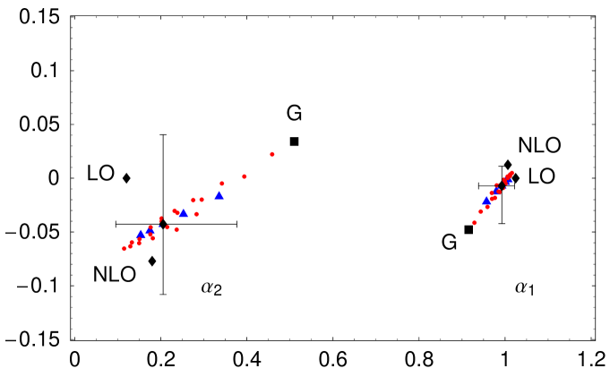
Figure 5: The tree amplitudes $\alpha_{1}(\pi\pi)$ and $\alpha_{2}(\pi\pi)$ represented in the complex plane. The dark (black) diamonds show the LO, NLO, and partial NNLO approximations. The latter includes the new 1-loop correction to spectator scattering and is shown with error bars. The dark square represents the parameter set ‘G’, which provides a good description of the experimental data on branching fractions as discussed in Section 5.3. The grey (blue) triangles show the variation of the tree amplitudes, when $\lambda_{B}$ takes the values $0.2\,$GeV to $0.5\,$GeV in steps of $75\,$MeV, such that the triangles in the direction of the point ‘G’ correspond to smaller values of $\lambda_{B}$. From each triangle emanates a set of grey (red) points that correspond to varying $a_{2}^{\pi}$ from $-0.1$ to 0.3 in steps of 0.1 for the given value of $\lambda_{B}$. Here points lying towards ‘G’ correspond to larger $a_{2}^{\pi}$.

5.3 $B\to\pi\pi$ branching fractions

We confront our new (partial) NNLO results with the experimental data on the three tree-dominated $B\to\pi\pi$ branching ratios. The $B\to\pi\pi$ amplitudes are given by

$$\sqrt{2}\,{\cal A}_{B^{-}\to\pi^{-}\pi^{0}} = i\,\frac{G_{F}}{\sqrt{2}}m_{B}^{2}f_{\pi}f^{B\pi}_{+}(0)V_{ub}V_{ud}^{*}\Big{[}\alpha_{1}+\alpha_{2}\Big{]},$$

$${\cal A}_{\bar{B}^{0}\to\pi^{+}\pi^{-}} = i\,\frac{G_{F}}{\sqrt{2}}m_{B}^{2}f_{\pi}f^{B\pi}_{+}(0)\left\{V_{ub}V_{ud}^{*}\Big{[}\alpha_{1}+\hat{\alpha}_{4}^{u}\Big{]}+V_{cb}V_{cd}^{*}\,\hat{\alpha}_{4}^{c}\right\},$$

$$-\,{\cal A}_{\bar{B}^{0}\to\pi^{0}\pi^{0}} = i\,\frac{G_{F}}{\sqrt{2}}m_{B}^{2}f_{\pi}f^{B\pi}_{+}(0)\left\{V_{ub}V_{ud}^{*}\Big{[}\alpha_{2}-\hat{\alpha}_{4}^{u}\Big{]}-V_{cb}V_{cd}^{*}\,\hat{\alpha}_{4}^{c}\right\},$$ (66)

not showing some smaller amplitudes that are taken into account in the numerical evaluation of the branching fractions below. The theoretical computation includes the 1-loop correction to spectator scattering in the tree amplitudes, $\alpha_{1,2}$, but not to the QCD penguin amplitudes $\hat{\alpha}_{4}^{u,c}$. For these (and the smaller amplitudes not shown) the NLO expression [1, 3] updated to include the scale-dependent parameters $a_{2}^{\pi}$ and $\hat{f}_{B}$ in the LO approximation for spectator scattering is used.

The standard input parameter set does not provide an adequate description of $B\to\pi\pi$ data. Rather the data favours a smaller value of $|V_{ub}|\,f^{B\pi}_{+}(0)$, which reduces the overall normalization of the amplitudes, and a significantly larger contribution from spectator scattering, which increases $\alpha_{2}$ (see Figure 5) [3]. We find that the parameter choice ‘G’ with

$$|V_{ub}|\,f^{B\pi}_{+}(0)=8.10\cdot 10^{-4}=0.775\,\Big{[}|V_{ub}|\,f^{B\pi}_{+}(0)\Big{]}_{\rm def},\qquad r_{\rm sp}=1.96\,[r_{\rm sp}]_{\rm def}$$ (67)

and $a_{2}^{\pi}(2\,\mbox{GeV})=0.3$ yields a good description of data. The required parameter modification is most likely related to a smaller value for the $B\to\pi$ form factor and a smaller value of $\lambda_{B}$, but other small modifications may add up to the combined effect. The new parameter selection ‘G’ is similar to scenario S4 defined in [3], and falls within the ranges for the individual parameters specified in Table 1. With (67) we calculate the CP-averaged branching fractions

$$10^{6}\,\mbox{Br}(B^{-}\to\pi^{-}\pi^{0}) = 5.5^{+0.3}_{-0.3}(\mbox{CKM})^{+0.5}_{-0.4}(\mbox{hadr.})^{+0.9}_{-0.8}(\mbox{pow.})\qquad[5.5\pm 0.6],$$

$$10^{6}\,\mbox{Br}(\bar{B}^{0}\to\pi^{+}\pi^{-}) = 5.0^{+0.8}_{-0.9}(\mbox{CKM})^{+0.3}_{-0.5}(\mbox{hadr.})^{+1.0}_{-0.5}(\mbox{pow.})\qquad[5.0\pm 0.4],$$ (68)

$$10^{6}\,\mbox{Br}(\bar{B}^{0}\to\pi^{0}\pi^{0}) = 0.73^{+0.27}_{-0.24}(\mbox{CKM})^{+0.52}_{-0.21}(\mbox{hadr.})^{+0.35}_{-0.25}(\mbox{pow.})\qquad[1.45\pm 0.29]$$

with the experimental averages reproduced in brackets [20]. The corresponding tree amplitudes $\alpha_{1}=0.92-0.05i$ and $\alpha_{2}=0.51+0.03i$ are shown by the points marked ‘G’ in Figure  5, which implies that the ratio of the colour-suppressed to colour-allowed amplitude $C/T=\alpha_{2}/\alpha_{1}=0.55+0.07i$ is large. By construction the branching fractions with charged pions in the final state are in excellent agreement with data. The $B\to\pi^{0}\pi^{0}$ branching fraction is still somewhat low, but the theoretical uncertainty is large. In computing the theoretical errors we did not include here the uncertainties in $|V_{ub}|$, $f_{+}^{B\pi}(0)$, $f_{B}$, $\lambda_{B}$ and $a_{2}^{\pi}$, because these 5 input parameters appear only through (67). The remaining uncertainties are divided into groups from $|V_{cb}|$, $\gamma$ (CKM); the renormalization scales $\mu_{\mathrm{hc}}$, $\mu_{b}$, and quark masses $m_{c}$, $m_{c}$ (hadr.); and $X_{H}$, $X_{A}$ (weak annihilation) parameterizing non-factorizable power corrections (pow.). The decays to the final states $\pi^{+}\pi^{-}$ and $\pi^{0}\pi^{0}$ are sensitive to $\gamma$ as can be seen from the CKM uncertainty. The dominant errors come from the hard-collinear factorization scale $\mu_{\mathrm{hc}}$, and from power corrections. We postpone a detailed assessment of the theoretical status after the calculation of the 1-loop spectator-scattering correction to the penguin amplitudes, which may be important for $\bar{B}^{0}\to\pi^{0}\pi^{0}$. We also expect the spectator-scattering phase in the penguin amplitudes to affect the direct CP asymmetries, and therefore do not discuss them now.

6 Conclusion

We computed the 1-loop hard spectator-scattering correction to the topological tree amplitudes in non-leptonic $B$ decays by matching the current-current operators $Q_{1,2}$ from the effective weak interaction Hamiltonian to the relevant operators in SCET_I. Together with the 1-loop calculation of the hard-collinear jet function [9, 10], the spectator-scattering contribution is now complete at order $\alpha_{s}^{2}$, also providing the first and perhaps dominant contribution to a full NNLO computation of the decay amplitudes. Unless the 1-loop term is enhanced by a large Wilson coefficient, it is of order $(30-50)\%$ relative to the tree term, depending on moments of light-cone distribution amplitudes. This yields a visible enhancement of the spectator-scattering amplitude without changing the qualitative features of the previous approximation.

The very fact that the perturbative correction can be computed, and that the expansion seems to be reasonably behaved, is significant, since it shows that a) factorization holds theoretically, i.e. IR singularities factorize as predicted and convolution integrals converge, and that b) perturbative expansions of the spectator-scattering contribution are under control, an issue that has at times been a point of controversy (second paper of [11], [22]). Our calculation therefore shows that the theoretical accuracy is now limited by the uncertainties of input parameters for the factorization formula, and encourages efforts to determine better key hadronic quantities such as form factors, and moments of light-cone distribution amplitudes.

Acknowledgements

We wish to thank D. Mueller for providing the 2-loop anomalous dimension matrix for the light-cone distribution amplitudes. M.B. would like to thank the INT, Seattle and KITP, Santa Barbara for their generous hospitality during the summer of 2004, when part of this work was being done. This work is supported in part by the DFG Sonderforschungsbereich/Transregio 9 “Computergestützte Theoretische Teilchenphysik”.

References

-
[1]
M. Beneke, G. Buchalla, M. Neubert and C. T. Sachrajda,
Phys. Rev. Lett. 83 (1999) 1914
[hep-ph/9905312];
M. Beneke, G. Buchalla, M. Neubert and C. T. Sachrajda, Nucl. Phys. B 591 (2000) 313 [hep-ph/0006124];
M. Beneke, G. Buchalla, M. Neubert and C. T. Sachrajda, Nucl. Phys. B 606 (2001) 245 [hep-ph/0104110]. -
[2]
C. N. Burrell and A. R. Williamson,
Phys. Rev. D 64 (2001) 034009
[hep-ph/0101190];
T. Becher, M. Neubert and B. D. Pecjak, Nucl. Phys. B 619 (2001) 538 [hep-ph/0102219];
M. Neubert and B. D. Pecjak, JHEP 0202 (2002) 028 [hep-ph/0202128];
C. N. Burrell and A. R. Williamson, [hep-ph/0504024]. - [3] M. Beneke and M. Neubert, Nucl. Phys. B 675 (2003) 333 [hep-ph/0308039].
- [4] M. Beneke and V. A. Smirnov, Nucl. Phys. B 522 (1998) 321 [hep-ph/9711391].
-
[5]
C. W. Bauer, S. Fleming, D. Pirjol and I. W. Stewart,
Phys. Rev. D 63 (2001) 114020
[hep-ph/0011336];
C. W. Bauer, D. Pirjol and I. W. Stewart, Phys. Rev. D 65 (2002) 054022 [hep-ph/0109045];
M. Beneke, A. P. Chapovsky, M. Diehl and Th. Feldmann, Nucl. Phys. B 643 (2002) 431 [hep-ph/0206152];
M. Beneke and Th. Feldmann, Phys. Lett. B 553 (2003) 267 [hep-ph/0211358];
R. J. Hill and M. Neubert, Nucl. Phys. B 657 (2003) 229 [hep-ph/0211018]. - [6] M. Beneke and T. Feldmann, Nucl. Phys. B 685 (2004) 249 [hep-ph/0311335].
-
[7]
C. W. Bauer, D. Pirjol and I. W. Stewart,
Phys. Rev. D 67 (2003) 071502
[hep-ph/0211069];
B. O. Lange and M. Neubert, Nucl. Phys. B 690 (2004) 249 [Erratum-ibid. B 723 (2005) 201] [hep-ph/0311345]. - [8] M. Beneke, Y. Kiyo and D. s. Yang, Nucl. Phys. B 692 (2004) 232 [hep-ph/0402241].
-
[9]
R. J. Hill, T. Becher, S. J. Lee and M. Neubert,
JHEP 0407 (2004) 081
[hep-ph/0404217];
T. Becher and R. J. Hill, JHEP 0410 (2004) 055 [hep-ph/0408344];
G. G. Kirilin, [hep-ph/0508235]. - [10] M. Beneke and D. Yang, to appear in Nuclear Physics B [hep-ph/0508250].
-
[11]
J. Chay and C. Kim,
Nucl. Phys. B 680 (2004) 302
[hep-ph/0301262];
C. W. Bauer, D. Pirjol, I. Z. Rothstein and I. W. Stewart, Phys. Rev. D 70 (2004) 054015 [hep-ph/0401188]. - [12] M. Beneke and M. Neubert, Nucl. Phys. B 651 (2003) 225 [hep-ph/0210085].
-
[13]
A. J. Buras and P. H. Weisz,
Nucl. Phys. B 333 (1990) 66;
A. J. Buras, M. Jamin, M. E. Lautenbacher and P. H. Weisz, Nucl. Phys. B 400 (1993) 37 [hep-ph/9211304]. - [14] G. Duplancic and B. Nizic, Eur. Phys. J. C 20 (2001) 357 [hep-ph/0006249].
- [15] M. J. Dugan and B. Grinstein, Phys. Lett. B 256 (1991) 239.
-
[16]
G. P. Lepage and S. J. Brodsky,
Phys. Rev. D 22 (1980) 2157;
A. V. Efremov and A. V. Radyushkin, Phys. Lett. B 94 (1980) 245. -
[17]
E. G. Floratos, D. A. Ross and C. T. Sachrajda,
Nucl. Phys. B 129 (1977) 66
[Erratum-ibid. B 139 (1978) 545];
D. Mueller, Phys. Rev. D 49 (1994) 2525;
A. V. Belitsky, D. Mueller, L. Niedermeier and A. Schäfer, Nucl. Phys. B 546 (1999) 279 [hep-ph/9810275]. -
[18]
V. M. Braun, D. Y. Ivanov and G. P. Korchemsky,
Phys. Rev. D 69 (2004) 034014
[hep-ph/0309330];
A. Khodjamirian, T. Mannel and N. Offen, Phys. Lett. B 620 (2005) 52 [hep-ph/0504091];
A. G. Grozin and M. Neubert, Phys. Rev. D 55 (1997) 272 [hep-ph/9607366];
S. J. Lee and M. Neubert, Phys. Rev. D 72 (2005) 094028 [hep-ph/0509350]. - [19] M. Beneke and S. Jäger, to appear in the Proceedings of the International Europhysics Conference on High Energy Physics, July 21st - 27th 2005, Lisboa, Portugal [hep-ph/0512101].
-
[20]
Heavy Flavour Averaging Group,
http://www.slac.stanford.edu/xorg/hfag/index.html - [21] X. q. Li and Y. d. Yang, Phys. Rev. D 72 (2005) 074007 [hep-ph/0508079].
- [22] M. Beneke, G. Buchalla, M. Neubert and C. T. Sachrajda, Phys. Rev. D 72 (2005) 098501 [hep-ph/0411171].