DO-TH 05/12

hep-ph/0512306

The Polarized and Unpolarized
Photon Content of the
Nucleon

Dissertation
zur Erlangung des Grades eines
Doktors der Naturwissenschaften
der Abteilung Physik
der Universität Dortmund

vorgelegt von

Cristian Pisano

Mai 2005

Chapter 1 Introduction

In this thesis the polarized and unpolarized photon distributions of the nucleon (proton, neutron), evaluated in the equivalent photon approximation, are computed theoretically and the possibility of their experimental determination is demonstrated. The thesis is based on the following publications [1, 2, 3, 4, 5, 6]:

• M. Glück, C. Pisano, E. Reya, The polarized and unpolarized photon content of the nucleon, Phys. Lett. B 540, 75 (2002) [Chapter 3].

• M. Glück, C. Pisano, E. Reya, I. Schienbein, Delineating the polarized and unpolarized photon distributions of the nucleon in $eN$ collisions, Eur. Phys. J. C 27, 427 (2003) [Chapter 4].

• A. Mukherjee, C. Pisano, Manifestly covariant analysis of the QED Compton process in $ep\rightarrow e\gamma p$ and $ep\rightarrow e\gamma X$, Eur. Phys. J. C 30, 477 (2003) [Chapter 5].

• A. Mukherjee, C. Pisano, Suppressing the background process to QED Compton scattering for delineating the photon content of the proton, Eur. Phys. J. C 35, 509 (2004) [Chapter 6].

• A. Mukherjee, C. Pisano, Accessing the longitudinally polarized photon content of the proton, Phys. Rev. D 70 , 034029 (2004) [Chapter 7].

• C. Pisano, Testing the equivalent photon approximation of the proton in the process $ep\rightarrow\nu WX$, Eur. Phys. J. C 38, 79 (2004) [Chapter 8].

The results of [5] have been summarized in [7] as well. Furthermore in Section 2.5 we shortly recall the main findings of the recent paper [8], also concerning the structure of the nucleon:

• M. Glück, C. Pisano, E. Reya, Probing the perturbative NLO parton evolution in the small-$x$ region, Eur. Phys. J. C 40, 515 (2005).

The equivalent photon approximation (EPA) of a charged fermion is a technical device which allows for a rather simple and efficient calculation of any photon-induced subprocess. The first explicit formulation and quantitative application of the EPA were given in 1924 by Fermi [9], who utilized it to estimate the electro-excitation and electro-ionization of atoms, and also the energy loss, due to ionization, of $\alpha$-particles travelling through matter. In several cases, he obtained a satisfactory numerical agreement with experimental data. Ten years later, in order to simplify calculations of processes involving relativistic collisions of charged particles, Williams [10] and Weizsäcker [11] further developed Fermi’s semi-classical treatment and extended it to high-energy electrodynamics. They observed that the electromagnetic field generated at a given point by a fast charged particle passing close to it contains predominantly transverse components. By making a Fourier analysis of the field, they concluded that the incident particle would produce the same effects as a beam of photons and computed their distribution in energy. This model assumes that the particle motion is not appreciably affected during the interaction, in particular that its scattering angle is small.

The first field-theoretical derivations were given in the fifties by Dalitz and Yennie [12], Curtis [13], Kessler and Kessler [14], and later by Chen and Zerwas [15]. The equivalent photon method for pointlike fermions, like the electron, has been investigated and utilized widely, for example it has been applied to pion production in electro-nucleon collisions [12, 13] and to two-photon processes for particle production at high energies [17, 16, 18]. A detailed history of the method, its various formulations and its first applications are contained in Kessler’s review article [19]. In more recent times, the validity of this approximation has been examined by Bawa and Stirling [20] in the context of the production of large transverse momentum photons at the HERA collider, by comparing the exact and approximate cross sections. Frixione, Mangano, Nason and Ridolfi in a well-known paper [21] further modified the method in order to improve its accuracy and tested it in the case of heavy-quark electroproduction at HERA. Their results were extended by De Florian and Frixione [22] to the case of a longitudinally polarized electron.

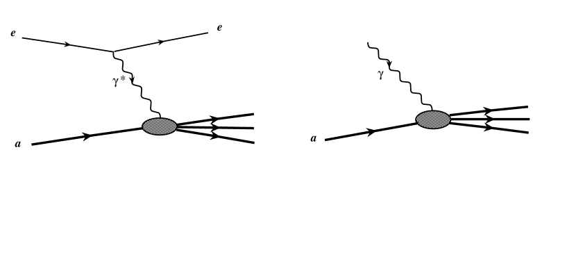
Figure 1.1: Connection between electroproduction and photoproduction on a target $a$.

As an example to illustrate the EPA, we shall consider the process in which an electron $e$ of very high energy scatters from a target hadron $a$, e.g. a proton. At leading order in $\alpha$, the fine structure constant of quantum electrodynamics (QED), the electron is connected to the target by one photon propagator, as depicted in the first diagram in Figure 1.1. If we denote with $E$ and $E^{\prime}$ respectively the initial and final energies of the electron, the photon will carry a momentum $q$ such that

$$q^{2}\simeq-2EE^{\prime}(1-\cos\theta),$$ (1.1)

where $\theta$ is the electron scattering angle. In the limit of forward scattering, whatever the energy loss, the photon momentum approaches $q^{2}=0$; therefore the reaction is highly peaked in the forward direction and the underlying dynamics is that of a photoproduction process. It can be shown that the cross section $\sigma_{ea}$, integrated over $q^{2}$ with integration bounds

$$q^{2}_{\rm{max}}=-\frac{m_{e}^{2}x^{2}}{1-x}~{},~{}~{}~{}~{}~{}~{}~{}~{}~{}~{}~{}~{}~{}q^{2}_{\rm{min}}\equiv-\mu^{2},$$ (1.2)

is given by a convolution of the probability that the electron radiates off a photon, the equivalent photon distribution $\gamma^{e}(x,\mu^{2})$, with the corresponding real photoproduction cross section $\sigma_{\gamma a}$, which is in general easier to calculate than the original one:

$${\operatorname{d}}\sigma_{ea}=\gamma^{e}(x,\mu^{2})\,\sigma_{\gamma a}{\operatorname{d}}x.$$ (1.3)

The connection between electroproduction and photoproduction on a target hadron $a$ is shown, in terms of Feynman diagrams, in Figure 1.1. An explicit expression of $\gamma^{e}(x,\mu^{2})$ is given in [21],

$$\gamma^{e}(x,\mu^{2})=\frac{\alpha}{2\pi}\bigg{[}\frac{1+(1-x)^{2}}{x}\,\ln\frac{\mu^{2}(1-x)}{m_{e}^{2}x^{2}}+2m_{e}^{2}x\bigg{(}\frac{1}{\mu^{2}}-\frac{1-x}{m_{e}^{2}x^{2}}\bigg{)}\bigg{]},$$ (1.4)

where $x$ is the fraction of the electron energy carried by the photon and $\mu$ has to be identified with a momentum scale of the photon-induced subprocess. While $q^{2}_{\rm max}$ in (1.2) is the largest value of $q^{2}$ kinematically allowed, $q^{2}_{\rm min}$ is not a well defined quantity, since when the momentum transfer squared becomes too large (in absolute value), the EPA breaks down and use of (1.3) would lead to huge errors. Critical examination of the EPA in electron-hadron collisions, in connection with different choices for the scale $\mu$, can be found in [20, 21].

The longitudinally polarized electron-target $a$ cross section $\Delta\sigma_{ea}$ can be obtained from (1.3) with the formal substitutions

$$\sigma\rightarrow\Delta\sigma,~{}~{}~{}\gamma^{e}\rightarrow\Delta\gamma^{e}.$$ (1.5)

The quantities $\Delta\sigma$ are defined in terms of cross sections $\sigma_{\lambda_{1}\lambda_{2}}$ for incoming particles of definite helicities,

$${\operatorname{d}}\Delta\sigma = \frac{1}{4}\,\,({\operatorname{d}}\sigma_{++}+{\operatorname{d}}\sigma_{--}-{\operatorname{d}}\sigma_{+-}-{\operatorname{d}}\sigma_{-+})$$ (1.6)

$$= \frac{1}{2}\,({\operatorname{d}}\sigma_{++}-{\operatorname{d}}\sigma_{+-}),$$

where the second equality follows from parity invariance of the electromagnetic interaction. The corresponding unpolarized cross section is obtained by taking the sum instead, namely

$$\sigma=\frac{1}{2}\,({\operatorname{d}}\sigma_{++}+{\operatorname{d}}\sigma_{+-}).$$ (1.7)

The polarized equivalent photon distribution $\Delta\gamma^{e}$ are defined in terms of densities for photons of definite helicity in electrons of definite helicity

$$\Delta\gamma^{e}=\gamma^{e+}_{+}-\gamma^{e+}_{-}=\gamma^{e-}_{-}-\gamma^{e-}_{+},$$ (1.8)

while the sum will give the unpolarized photon distribution,

$$\gamma^{e}=\gamma^{e+}_{+}+\gamma^{e+}_{-}=\gamma^{e-}_{-}+\gamma^{e-}_{+},$$ (1.9)

where the superscripts refer to the parent electron and the subscripts to the photon. One can show that [22]

$$\Delta\gamma^{e}(x,\mu^{2})=\frac{\alpha}{2\pi}\bigg{[}\frac{1-(1-x)^{2}}{x}\,\ln\frac{\mu^{2}(1-x)}{m_{e}^{2}x^{2}}+2m_{e}^{2}x^{2}\bigg{(}\frac{1}{\mu^{2}}-\frac{1-x}{m_{e}^{2}x^{2}}\bigg{)}\bigg{]}.$$ (1.10)

In the treatment of protons and neutrons, (1.3) and (1.5)-(1.9) still hold, with the replacement $e\rightarrow p$ or $n$, but a special situation arises in the calculation of their photon distributions, due to the fact that they are not pointlike particles. Here it is necessary to distinguish between elastic and inelastic scattering. In the former case the nucleon does not break up but is temporaly in an excited state, which can be described in terms of certain form factors. In the latter case, appealing to the parton model, only quarks, antiquarks and gluons are usually considered as the (essentially free) constituents of the initial nucleon, which ceases to exist and its constituents finally hadronize. The photons radiated off the quarks and antiquarks may be characterized by (1.4) and (1.10), and due to their logarithmic enhancement factor they are expected to become increasingly relevant at very high energies, when the momentum scale $\mu$ is also large. At this level the “inelastic” photons can be included among the parton distributions of the nucleon.

Therefore the total (polarized) unpolarized photon distribution of a nucleon $N$ will be given by

$$(\Delta)\gamma(x,\mu^{2})=(\Delta)\gamma_{\mathrm{el}}(x)+(\Delta)\gamma_{\mathrm{inel}}(x,\mu^{2}),$$ (1.11)

where the elastic component $(\Delta)\gamma_{\rm el}$ is due to $N\to\gamma N$ and the inelastic component $(\Delta)\gamma_{\mathrm{inel}}$ is due to $N\to\gamma X$ with $X\neq N$. As pointed out by Drees and Zeppenfeld [23] and by Kniehl [24], $\gamma^{p}_{\rm el}$ cannot be obtained from (1.4) by just replacing the electron mass with the proton mass: this would strongly overestimate it. One has to take into account the effects of the form factors, which determine the scale independence of $(\Delta)\gamma_{\rm el}$. The derivations of $\gamma^{p}_{\mathrm{el}}$ and $\gamma^{p}_{\mathrm{inel}}$, performed in [24] and by Glück, Stratmann, Vogelsang in [25], will be generalized to the neutron and to the polarized sector in Chapter 3.

The photon content of the nucleon $\gamma(x,\mu^{2})$ can be utilized, instead of the more common form factors and parton distributions, to calculate photon-induced subprocesses in elastic and deep inelastic $ep$ reactions, leading to great simplifications. For example, as shown by Blümlein [26] and by De Rújula and Vogelsang [27], the analysis of the deep inelastic QED Compton scattering process $ep\to e\gamma X$ reduces to the calculation of the $2\to 2$ subprocess $e\gamma^{p}\to e\gamma$ instead of having to calculate the full $2\to 3$ subprocess $eq\to e\gamma q$. Analogously one can consider just the simple $2\to 2$ subprocess $\gamma^{e}\gamma^{p}\to\mu^{+}\mu^{-}$ (instead of $\gamma^{e}q\rightarrow\mu^{+}\mu^{-}q$) for the analysis of deep inelastic $ep\to\mu^{+}\mu^{-}X$, or $e\gamma^{p}\to\nu W$ (instead of $eq\rightarrow\nu Wq$) for associated $\nu W$ production in $ep\to\nu WX$.

Similarly, $\gamma\gamma$ fusion processes like $\gamma^{p}\gamma^{p}\to\ell^{+}\ell^{-},\,c\bar{c},\,H^{+}H^{-},\,\tilde{\ell}^{+}\tilde{\ell}^{-}$ for (heavy) lepton ($\ell$), heavy quark ($c$), charged Higgs ($H^{\pm}$) and slepton ($\tilde{\ell}$) production can be easily analyzed in purely hadronic $pp$ reactions, providing also an interesting possibility of producing charged particles which do not have strong interactions. Carlson and Lassila [28], Drees, Godbole, Nowakowski, Rindani [29], and Ohnemus, Walsh, Zerwas [30] initiated these studies; in particular, in [29] it is shown that the cross section for the pair production of heavy charged scalars or fermions via $\gamma\gamma$ fusion amounts to a few percent of the corresponding Drell-Yan $q\bar{q}$ annihilation cross sections, at energies reached at the CERN Large Hadron Collider (LHC). However, the disadvantage of the low production rates is compensated by the simple and clean experimental situation encountered when the photons are emitted from protons which do not break up (purely elastic processes) [30].

It still remains to extend the above-mentioned analysis to $pd$ and $dd$ reactions. Moreover, analogous remarks hold for the longitudinally polarized $\vec{e}\vec{N}$ and $\vec{p}\vec{p},\,\vec{p}\vec{d}$, $\vec{d}\vec{d}$ reactions where the polarized photon content of the nucleon $\Delta\gamma(x,\mu^{2})$ enters.

In this thesis we shall concentrate on lepton-nucleon scattering, with special attention to the aforementioned QED Compton process, which is one of the most important reactions for directly measuring the photon content of the nucleon and testing the reliability of the EPA. Furthermore, we shall discuss how such measurements can provide additional, independent informations concerning the usual polarized and unpolarized structure functions, along the lines of [26, 31, 33, 32].

In detail, the outline of the thesis will be as follows:

• Chapter 2 serves as an introduction into the concepts of electromagnetic form factors, structure functions and parton distributions of the nucleon, in terms of which elastic and inelastic $eN$ cross sections are commonly expressed. They are presented here because they enter in the definition of the photon content of the nucleon. Notations and conventions used in this chapter as well as in the rest of the thesis are summarized in Appendix A.

• In Chapter 3 a new expression for the polarized equivalent photon distribution is explicitly derived. The calculation of the unpolarized one, already performed in [24, 25, 27], is also shown in detail for completeness and the resulting photon asymmetries are presented for some typical relevant momentum scales.

• The production rates of lepton-photon and dimuon pairs at the HERA collider and HERMES experiment are evaluated in Chapter 4, utilizing the photon distributions previously derived, convoluted with the cross sections relative to the subprocesses $e\gamma\to e\gamma$ and $\gamma\gamma\to\mu^{+}\mu^{-}$, given in Appendix B. It is shown that the production rates are sufficient to measure the polarized and unpolarized photon content of the nucleon.

• Chapter 5 is devoted to the unpolarized QED Compton scattering in $ep\rightarrow e\gamma p$ and $ep\rightarrow e\gamma X$, with the photon emitted from the lepton. The full $2\rightarrow 3$ process is calculated in a manifestly covariant way by employing appropriate parametrizations of the proton’s structure functions. These results are compared with the ones based on the EPA, as well as with the experimental data and theoretical estimates for the HERA collider given in [31]. It is shown that the cross section is reasonably well described by the EPA of the proton, also in the inelastic channel. In addition it turns out that the results obtained in [31], based on an iterative approximation procedure proposed by Courau and Kessler [34], deviate appreciably from our analysis in certain kinematical regions. Details about the kinematics of the process are given in Appendix C.

• In Chapter 6 the virtual Compton scattering process in $ep\rightarrow e\gamma p$ and $ep\rightarrow e\gamma X$, where the photon is emitted from the hadronic vertex, is investigated. It represents the major background process to QED Compton scattering. New kinematical cuts are suggested in order to suppress the virtual Compton scattering background and facilitate the extraction of the equivalent photon distribution of the proton at the HERA collider. The analytic expressions of the matrix elements of unpolarized QED and virtual Compton scattering can be found in Appendix D.

• Chapter 7 is devoted to the QED Compton process in longitudinally polarized lepton-proton scattering. The kinematical cuts necessary to measure the polarized photon content of the proton and to suppress the major background process coming from Virtual Compton scattering are provided for HERMES, COMPASS and future eRHIC experiments. We point out that these measurements will also give access to the spin dependent structure function $g_{1}$ in a kinematical region not well covered by inclusive measurements. The analytic expressions of the matrix elements of polarized QED and virtual Compton scattering are relegated to Appendix E.

• The accuracy of the EPA of the proton in describing the inelastic process $ep\rightarrow\nu WX$ is investigated in Chapter 8. In particular, the scale dependence of the corresponding inelastic photon distribution is discussed. Furthermore, an estimate of the total number of events, including the ones coming from the elastic and quasi-elastic channels of the reaction, is given for the HERA collider.

• Finally, summary and conclusions can be found in Chapter 9.

Chapter 2 The Structure of the Nucleon

In physics, one of the most common ways of getting information on the structure of extended objects like hadrons is to use structureless particles as projectiles which scatter off the hadron in question. To probe the inside of a nucleon one naturally uses charged lepton (electron or muon) beams: such reactions dominantly take place by the exchange of a single virtual photon, therefore they can be studied with relative ease and clarity. Effects of higher order virtual photon exchange are believed to be less than a few percent.
According to Heisenberg’s uncertainty principle, one can resolve the target structure down to the scale $\lambda\sim\hbar/Q$, where $Q$ is the momentum transfer from the lepton to the nucleon. Hence, the higher the energy loss of the lepton, the finer the structure that can be resolved. The study of such reactions represent the main subject of the present chapter.

In Section 2.1 we examine electron-nucleon elastic scattering and discuss the significance of the electromagnetic form factors. In Section 2.2 inelastic electron-nucleon scattering is described in terms of the structure functions $F_{1}$ and $F_{2}$. The spin dependent structure functions $g_{1}$ and $g_{2}$ are introduced in Section 2.3. The parton model and quantum chromodynamics description of inelastic electron-nucleon collisions can be found in Section 2.4 and in Section 2.5 respectively.

Figure 2.1: The one-photon exchange diagram for elastic electron-nucleon scattering.

2.1 Elastic Form Factors

We consider the elastic electron-nucleon scattering process:

$$e(l)+N(P)\rightarrow e(l^{\prime})+N(P^{\prime}),$$ (2.1)

where the four-momenta of the particles are given in the brackets. At lowest order in perturbation theory of QED the reaction is described by a one-photon exchange diagram, depicted in Figure 2.1. In terms of the Dirac $\gamma$ matrices and spinors, the electron transition current is

$$\langle\,e(l^{\prime})\,|\,J^{\alpha}_{\mathrm{em}}(0)\,|\,e(l)\,\rangle=-e\,[\,\bar{u}(l^{\prime})\,\gamma^{\alpha}\,u(l)\,],$$ (2.2)

with $e$ denoting the electric charge of the proton. The vertex linking the photon with the nucleon is not point-like, therefore the nucleon transition current is different from (2.2); it is the most general Lorentz four-vector that can be constructed from $P$, $P^{\prime}$ and the $\gamma$ matrices, sandwiched between $\bar{u}(P)$ and $u(P)$:

$$\langle\,N(P^{\prime})\,|\,J^{\alpha}(0)\,|\,N(P)\,\rangle=e\,[\,\bar{u}(P^{\prime})\,\Gamma^{\alpha}\,u(P)\,].$$ (2.3)

In $\Gamma^{\alpha}$ terms involving $\gamma^{5}$ are ruled out by the conservation of parity. Furhermore, using the Dirac equations $P\!\!\!\!/\,u(P)=mu(P)$ and $\bar{u}(P^{\prime})P^{\prime}\!\!\!\!\!/\,=m\bar{u}(P^{\prime})$, where $m$ is the nucleon mass, one can show that there are only three independent terms, $\gamma^{\alpha}$, $i\sigma^{\alpha\beta}q_{\beta}$ and $q^{\alpha}$, with

$$\sigma^{\alpha\beta}=\frac{i}{2}\,[\gamma^{\alpha},\,\gamma^{\beta}]$$ (2.4)

and $q$ being the momentum transfer,

$$q=l-l^{\prime}.$$ (2.5)

Therefore, quite generally,

$$\Gamma^{\alpha}=F_{1}(q^{2})\gamma^{\alpha}+\frac{1}{2m}F_{2}(q^{2})i\sigma^{\alpha\beta}q_{\beta}+F_{3}(q^{2})q^{\alpha}.$$ (2.6)

The coefficients $F_{k}(q^{2})$ ($k=1,2,3$) are the electromagnetic elastic form factors of the nucleon, which are functions of the momentum transfer squared $q^{2}$, the only independent scalar variable at the nucleon vertex (being $P\cdot q=-q^{2}/2$). For the electromagnetic case we are interested in, $J^{\alpha}_{\mathrm{em}}$ is a conserved current and therefore the matrix element (2.3) has to satisfy the condition

$$q_{\alpha}\,\langle\,N(P^{\prime})\,|\,J^{\alpha}_{\mathrm{em}}\,|\,N(P)\,\,\rangle=0,$$ (2.7)

which implies $F_{3}(q^{2})=0$ in (2.6). The Dirac equation can be used again in order to replace $\bar{u}(P^{\prime})i\,\sigma^{\alpha\beta}q_{\beta}u(P)$ by $\bar{u}(P^{\prime})[2\,m\gamma^{\alpha}-(P+P^{\prime})^{\alpha}]u(P)$ in (2.6) so that one can write

$$\Gamma_{\mathrm{em}}^{\alpha}=(\,F_{1}(q^{2})+F_{2}(q^{2})\,)\,\gamma^{\alpha}-\frac{1}{2m}\,F_{2}(q^{2})\,(P+{P^{\prime}})^{\alpha}\,.$$ (2.8)

At $q^{2}=0$, which physically corresponds to the nucleon interacting with a static electro-magnetic field, the form factors are related to the electric charge $Q$ and the magnetic dipole moment $\mu$ of the nucleon:

$$eF_{1}(0)=Q,~{}~{}~{}~{}~{}~{}~{}\frac{e}{2m}\,[F_{1}(0)+F_{2}(0)]=\mu.$$ (2.9)

For an electrically neutral particle, like the neutron, one has $F_{1}(0)$ = 0. If a particle has no anomalous magnetic moment $\kappa$, defined such that $\mu=(1+\kappa)\,e/(2m)$, then $F_{2}(0)=0$. Experimentally,

$$F_{1}^{p}(0)=1,~{}~{}~{}~{}~{}~{}~{}F_{2}^{p}(0)=\kappa_{p}\simeq 1.79$$ (2.10)

for the proton, and

$$F_{1}^{n}(0)=0,~{}~{}~{}~{}~{}~{}~{}F_{2}^{n}(0)=\kappa_{n}\simeq-1.91$$ (2.11)

for the neutron. In the following, we will always express $\mu$ in units of the nucleon magneton $e\hbar/(2mc)$, that is $\mu_{p}=2.79$, $\mu_{n}=-1.91$.

The amplitude $M$ relative to the process (2.1) has the form

$$M=-e^{2}\,[\bar{u}(l^{\prime})\gamma_{\alpha}u(l)]\,\frac{1}{q^{2}}\,[\bar{u}(P^{\prime})\Gamma_{\mathrm{em}}^{\alpha}u(P)].$$ (2.12)

Taking the modulus squared of the amplitude and multiplying by the appropriate phase space and flux factors, one finds that the differential cross section can be written as

$${\operatorname{d}}\sigma=\frac{1}{4\sqrt{(l\cdot P)^{2}-m^{2}m_{e}^{2}}}\,\overline{|M|^{2}}\,(2\pi)^{4}\delta^{4}(l+P-l^{\prime}-P^{\prime})\,\frac{{\operatorname{d}}^{3}{\mbox{\boldmath$l$}}^{\prime}}{(2\pi)^{3}\,2l^{\prime}_{0}}\,\frac{{\operatorname{d}}^{3}{\mbox{\boldmath$P$}}^{\prime}}{(2\pi)^{3}\,2P^{\prime}_{0}}~{},$$ (2.13)

which holds with the normalization of the spinors given in (A.16) and where $m_{e}$ denotes the electron mass. After integrating over the phase space of the scattered nucleon, one can use the condition ${\mbox{\boldmath$P$}}^{\prime}={\mbox{\boldmath$P$}}+{\mbox{\boldmath$q$}}$ to rewrite the energy conserving $\delta$-function as

$$\frac{1}{2P^{\prime}_{0}}\,\delta(l_{0}+P_{0}-l^{\prime}_{0}-P^{\prime}_{0}) = \delta({P^{\prime}_{0}}^{2}-(P_{0}+q_{0})^{2})\,=\,\delta(P^{\prime 2}-(P+q)^{2})$$ (2.14)

$$= \delta(q^{2}+2P\cdot q).$$

Therefore (2.13) reduces to

$${\operatorname{d}}\sigma=\frac{1}{4\sqrt{(l\cdot P)^{2}-m^{2}m_{e}^{2}}}\,\overline{|M|^{2}}\,\frac{{\operatorname{d}}^{3}{\mbox{\boldmath$l$}}^{\prime}}{(2\pi)^{2}\,2l^{\prime}_{0}}\,\delta(q^{2}+2P\cdot q),$$ (2.15)

with

$$\overline{|M|^{2}}=\frac{1}{q^{4}}\,L_{\alpha\beta}(l;l^{\prime})\,H_{\mathrm{el}}^{\alpha\beta}(P;P^{\prime}),$$ (2.16)

where the tensors $L_{\alpha\beta}(l;l^{\prime})$ and $H_{\mathrm{el}}^{\alpha\beta}(P;P^{\prime})$ come from averaging over initial spins and summing over final spins in the products of the electron and nucleon matrix elements (2.2) and (2.3), when (2.12) is squared. The completeness relation (A.17) is commonly used to perform the spin sums. More explicitly:

$$L^{\alpha\beta}(l;l^{\prime}) = \frac{1}{2}\sum_{\mathrm{spins}}\,{\langle e(l^{\prime})\mid J_{\mathrm{em}}^{\alpha}(0)\mid e(l)\rangle}^{*}\langle e(l^{\prime})\mid J_{\mathrm{em}}^{\beta}(0)\mid e(l)\rangle$$ (2.17)

$$= \frac{1}{2}\,e^{2}\,\mathrm{Tr}[(l^{\prime}\!\!\!\!/+m_{e})\gamma^{\alpha}(l\!\!\!/+m_{e})\gamma^{\beta}]$$

$$= 2\,e^{2}\{l^{\alpha}l^{\prime\beta}+l^{\prime\alpha}l^{\beta}-g^{\alpha\beta}(l\cdot l^{\prime}-m_{e}^{2})\}$$

and

$$H^{\alpha\beta}_{\mathrm{el}}(P;P^{\prime}) = \frac{1}{2}\sum_{\mathrm{{spins}}}\,{\langle N(P^{\prime})\mid J_{\mathrm{em}}^{\alpha}(0)\mid N(P)\rangle}^{*}\langle N(P^{\prime})\mid J_{\mathrm{em}}^{\beta}(0)\mid N(P)\rangle$$ (2.18)

$$= \frac{1}{2}\,e^{2}\,\mathrm{Tr}[(P^{\prime}\!\!\!\!\!/+m)\Gamma^{\alpha}(P\!\!\!\!/+m)\Gamma^{\beta}]$$

$$= e^{2}\,\bigg{[}\bigg{(}F_{1}^{2}-\frac{q^{2}}{4m^{2}}F_{2}^{2}\bigg{)}(P+P^{\prime})^{\alpha}(P+P^{\prime})^{\beta}$$

$$~{}~{}~{}~{}~{}~{}~{}~{}~{}~{}~{}~{}~{}~{}~{}~{}~{}~{}+(F_{1}+F_{2})^{2}(q^{2}g^{\alpha\beta}-q^{\alpha}q^{\beta})\bigg{]}.$$

In the kinematical region of high energies, the electron mass can be neglected and then the contraction of (2.17) and (2.18) gives

$$L_{\alpha\beta}(l;l^{\prime})H_{\mathrm{el}}^{\alpha\beta}(P;P^{\prime}) = 2e^{4}\bigg{\{}\,4\bigg{(}F_{1}^{2}-\frac{q^{2}}{4m^{2}}F_{2}^{2}\bigg{)}[\,2(P\cdot l^{\prime})(P\cdot l)-(l\cdot l^{\prime})m^{2}]$$ (2.19)

$$~{}~{}~{}~{}~{}~{}~{}~{}~{}~{}~{}~{}~{}~{}~{}~{}~{}~{}~{}-2(F_{1}+F_{2})^{2}\,q^{2}\,(l\cdot l^{\prime})\,\bigg{\}}.$$

In a frame in which the nucleon is at rest and the electron moves along the $z$ axis with energy $E$ and is scattered into a solid angle $\Omega=(\theta,\varphi)$ with final energy $E^{\prime}$, i.e.

$$P=(m,0,0,0,),~{}~{}~{}l=E(1,0,0,1),~{}~{}~{}l^{\prime}=E^{\prime}(1,\sin\theta\cos\varphi,\sin\theta\sin\varphi,\cos\theta),$$ (2.20)

then

$$q^{2}=(l-l^{\prime})^{2}=-4EE^{\prime}\sin^{2}\frac{\theta}{2}$$ (2.21)

and one can define the energy transfer from the electron to the target

$$\nu=E-E^{\prime}=\frac{q\cdot P}{m}~{}.$$ (2.22)

The differential cross section (2.15) can be rewritten as

$$\frac{{\operatorname{d}}\sigma}{{\operatorname{d}}E^{\prime}{\operatorname{d}}\Omega}=\frac{\alpha^{2}}{4E^{\prime 2}\sin^{4}\frac{\theta}{2}}\,\bigg{[}\bigg{(}F_{1}^{2}-\frac{q^{2}}{4m^{2}}F_{2}^{2}\bigg{)}\cos^{2}\frac{\theta}{2}-\frac{q^{2}}{2m^{2}}(F_{1}+F_{2})^{2}\sin^{2}\frac{\theta}{2}\,\bigg{]}\delta\bigg{(}\nu+\frac{q^{2}}{2m}\bigg{)},$$ (2.23)

with $\alpha=e^{2}/(4\pi)$. The form factors $F_{1}$ and $F_{2}$, usually referred to as the Dirac and Pauli form factors respectively, parametrize our ignorance of the complicated structure of the nucleon. In practice, however, it is better to use linear combinations of them, the Sachs electric and magnetic form factors

$$G_{E}(q^{2}) = F_{1}(q^{2})+\frac{q^{2}}{4m^{2}}F_{2}(q^{2}),$$

$$G_{M}(q^{2}) = F_{1}(q^{2})+F_{2}(q^{2}),$$ (2.24)

defined so that no interference terms, $G_{E}G_{M}$, occur in (2.23). At $q^{2}=0$, one has

$$G_{E}^{p}(0) = 1,~{}~{}~{}~{}~{}~{}~{}G_{M}^{p}(0)\,=\,1+\kappa_{p}\simeq 2.79,$$

$$G_{E}^{n}(0) = 0,~{}~{}~{}~{}~{}~{}~{}G_{M}^{n}(0)\,=\,\kappa_{n}\simeq-1.91.$$ (2.25)

Integration of (2.23) over $E^{\prime}$, taking into account that $q^{2}$ depends on $E^{\prime}$ when $\theta$ is held fixed, see (2.21), gives the Rosenbluth formula [35]

$$\frac{{\operatorname{d}}\sigma}{{\operatorname{d}}\Omega}=\frac{\alpha^{2}}{4E^{2}\sin^{4}\frac{\theta}{2}}\,\frac{E^{\prime}}{E}\,\bigg{(}\frac{G_{E}^{2}+\tau G_{M}^{2}}{1+\tau}\cos^{2}\frac{\theta}{2}+2\tau G_{M}^{2}\sin^{2}\frac{\theta}{2}\bigg{)},$$ (2.26)

with $\tau\equiv-q^{2}/4m^{2}$ and the factor

$$\frac{E^{\prime}}{E}=\bigg{(}1+\frac{2E}{m}\sin^{2}\frac{\theta}{2}\bigg{)}^{-1}$$ (2.27)

arises from the recoil of the target. The Rosenbluth formula is the basis of all experimental studies of the electromagnetic structure of the nucleon and allows to determine the form factors by measuring ${\operatorname{d}}\sigma/{\operatorname{d}}\Omega$ as a function of $\theta$ and $q^{2}$. Experimentally it turns out that the form factors drop rapidly as $-q^{2}$ increases:

$$G^{p}_{E}(q^{2})=\frac{G_{M}^{p}(q^{2})}{\mu_{p}}=\frac{G_{M}^{n}(q^{2})}{\mu_{n}}=\bigg{(}1-\frac{q^{2}}{0.71\,\mathrm{GeV}^{2}}\bigg{)}^{-2},$$ (2.28)

$$0\leq G_{E}^{n}(q^{2})\leq 0.1~{}.~{}~{}~{}~{}~{}~{}~{}~{}~{}~{}~{}~{}~{}~{}~{}~{}~{}~{}~{}~{}~{}~{}~{}~{}~{}~{}~{}~{}~{}~{}~{}~{}~{}~{}~{}~{}~{}~{}~{}~{}~{}~{}~{}~{}~{}$$ (2.29)

The function given in (2.28) is merely empirical and is often called a dipole fit; a monopole fit would be $(1-cq^{2})^{-1}$. Also there is no fundamental theoretical reason for $G_{E}^{p}$, $G_{M}^{p}$, $G_{E}^{n}$ to have the same $q^{2}$ behaviour: this likeness is expressed by saying that the three form factors scale together in $q^{2}$.

In the non-relativistic limit, $E\ll m$, one can see from (2.27) that $E=E^{\prime}$; therefore $-q^{2}=|$$q$$|^{2}$ $\ll m^{2}$. In this limit the form factors $G_{E}$ and $G_{M}$ are the Fourier transforms of the nucleon’s charge and magnetic moment density distributions, respectively [36]. Assuming, for example, that the charge density distribution of the proton is spherically symmetric, i.e. a function of $r\equiv|{\mbox{\boldmath$r$}}|$ alone, and that it is normalized such that

$$\int{\operatorname{d}}^{3}{\mbox{\boldmath$r$}}\,\rho({\mbox{\boldmath$r$}})=1,$$ (2.30)

then the exponential in its Fourier transform can be expanded for small $|{\mbox{\boldmath$q$}}|$ as follows

$$G^{p}_{E}(q^{2})=\int{\operatorname{d}}^{3}\,{\mbox{\boldmath$r$}}\rho(r)e^{i\,{{\mbox{\boldmath$q$}}\cdot{\mbox{\boldmath$r$}}}} = \int{\operatorname{d}}^{3}\,{\mbox{\boldmath$r$}}\rho(r)\bigg{(}1+i{{\mbox{\boldmath$q$}}\cdot{\mbox{\boldmath$r$}}}-\frac{{({\mbox{\boldmath$q$}}\cdot{\mbox{\boldmath$r$}})^{2}}}{2}+...\bigg{)}$$ (2.31)

$$= 1-\frac{1}{6}\,|{\mbox{\boldmath$q$}}|^{2}\,\langle r^{2}\rangle+...~{},$$

where the mean square charge radius of the proton is defined by

$$\langle r^{2}\rangle=\int{\operatorname{d}}^{3}{\mbox{\boldmath$r$}}\,\rho(r)r^{2}.$$ (2.32)

Identifying (2.31) with the expansion of (2.28),

$$G_{E}^{p}(q^{2})=G_{E}^{p}(0)+q^{2}\,\bigg{(}\frac{{\operatorname{d}}G_{E}^{p}(q^{2})}{{\operatorname{d}}q^{2}}\bigg{)}_{q^{2}=0}+...=1-|{\mbox{\boldmath$q$}}|^{2}\,\bigg{(}\frac{{\operatorname{d}}G_{E}^{p}(q^{2})}{{\operatorname{d}}q^{2}}\bigg{)}_{q^{2}=0}+...~{},$$ (2.33)

one gets

$$\langle r^{2}\rangle = \int{\operatorname{d}}^{3}{\mbox{\boldmath$r$}}\,\rho(r)r^{2}\,=\,6\,\bigg{(}\frac{{\operatorname{d}}G_{E}^{p}(q^{2})}{{\operatorname{d}}q^{2}}\bigg{)}_{q^{2}=0}$$ (2.34)

$$= (0.81\times 10^{-13}\mathrm{cm})^{2}.$$

The same radius of about 0.8 fm is obtained for the magnetic moment distribution. Finally, the charge distribution of the nucleon has an exponential shape in configuration space: the Fourier transform of $\rho(r)=e^{-mr}$, with $m=0.84$ ${\rm GeV}$, gives the result (2.28) for $G_{E}^{p}$.

Figure 2.2: The one-photon exchange diagram for inelastic electron-nucleon scattering.

2.2 Unpolarized Structure Functions

Probing the nucleon with a large wavelength photon (small momentum transfer squared $-q^{2}$) can only provide information about its dimension. It is possible to have a better spatial resolution by increasing $-q^{2}$, but already for $-q^{2}\gtrsim m^{2}$ the elastic process (2.1) is not dominant any more and the nucleon often breaks up into hadronic debris. The inelastic reaction

$$e(l)+N(P)\rightarrow e(l^{\prime})+X(P_{X}),$$ (2.35)

where $X$ is the undetected hadronic system, represents the most direct way to explore the internal structure of the nucleon; it is fully inclusive with respect to the hadronic state and, when the momentum transfer is not ultra-high, is dominated by one-photon exchange, as described by the diagram in Figure 2.2. The reaction (2.35) is described by three kinematic variables. One of them, the incoming lepton energy $E$, or alternatively the center-of-mass energy squared $s=(l+P)^{2}$, is fixed by the experimental conditions. The other two independent variables can be chosen among the following invariants: $Q^{2}\equiv-q^{2}$ and $\nu$, already defined in (2.21) and (2.22), the center-of-mass energy squared of the $\gamma^{*}N$ system (that is the invariant mass squared of the hadronic system $X$)

$$W^{2} = (P+q)^{2},$$ (2.36)

the Bjorken variable

$$x_{B} = \frac{Q^{2}}{2P\cdot q}=\frac{Q^{2}}{Q^{2}+W^{2}-m^{2}}~{},$$ (2.37)

and the “inelasticity”

$$y = \frac{P\cdot q}{P\cdot l}=\frac{W^{2}+Q^{2}-m^{2}}{s-m^{2}}~{}.$$ (2.38)

In the target rest frame, where $\nu$ is the transferred energy from the electron to the target, $y$ is the fraction of the incoming electron energy carried by the exchanged photon, $y=\nu/E$. The relation connecting $x_{B}$, $y$ and $Q^{2}$ is given by

$$x_{B}y=\frac{Q^{2}}{s-m^{2}}\simeq\frac{Q^{2}}{s}~{}.$$ (2.39)

Since $W^{2}\geq m^{2}$ the Bjorken variable $x_{B}$ takes values between 0 and 1, and so does $y$. The measurement of the cross section corresponding to the process (2.35) shows a peak when the nucleon does not break up ($W\simeq m$) and broader peaks when the target is excited to resonant barion states, most of them concentrated in the range $m\lesssim W\lesssim 1.8$ ${\rm GeV}$. As $W$ increases one reaches a region where a smooth behaviour is set in. This is the deep inelastic region, where both $Q$ and $W$ are large compared to the typical hadron masses. In this kinematical domain, the reaction (2.35) is known as deep inelastic scattering.

If we neglect the electron mass, the cross section for deep inelastic scattering (DIS) can be written as

$${\operatorname{d}}\sigma=\frac{1}{4P\cdot l}\,\frac{1}{Q^{4}}\,L_{\alpha\beta}(l;l^{\prime})W^{\alpha\beta}\,\frac{{\operatorname{d}}^{3}\mbox{\boldmath$l$}^{\prime}}{(2\pi)^{3}2l_{0}^{\prime}}~{},$$ (2.40)

where, as before, we have averaged over the initial electron and nucleon spins, and summed over the final electron spin. The leptonic tensor $L_{\alpha\beta}(l;l^{\prime})$ was calculated in (2.17) and the hadronic tensor, corresponding to the electromagnetic transitions of the target nucleon to all possible final states, is defined as

$$W^{\alpha\beta}=\sum_{X}\int\frac{{\operatorname{d}}^{3}{\mbox{\boldmath$P$}}_{X}}{(2\pi)^{3}2P^{0}_{X}}\,H^{\alpha\beta}_{\mathrm{inel}}(P;P_{X})(2\pi)^{4}\delta^{4}(l+P-l^{\prime}-P_{X}),$$ (2.41)

with

$$H^{\alpha\beta}_{\mathrm{inel}}(P;P_{X})={1\over 2}\sum_{\mathrm{{spins}}}{\langle X(P_{X})\mid J_{\mathrm{em}}^{\alpha}(0)\mid N(P)\rangle}^{*}\langle X(P_{X})\mid J_{\mathrm{em}}^{\beta}(0)\mid N(P)\rangle$$ (2.42)

and $P_{X}$ denoting the total four-momentum of the state $|X\rangle$. The definition (2.41) holds with states normalized as in (A.13). The cross section (2.40) reduces to (2.13), with $m_{e}=0$, when $X$ is restricted to be also a nucleon.

In general, if we do not average over the initial nucleon spin $S$, the electromagnetic hadronic tensor $W_{\alpha\beta}$ consists of a symmetric and an antisymmetric (spin dependent) part under $\alpha\leftrightarrow\beta$,

$$W_{\alpha\beta}=W^{\mathrm{S}}_{\alpha\beta}(q,P)+W^{\mathrm{A}}_{\alpha\beta}(q;P,S).$$ (2.43)

Since $J^{\alpha}_{\rm{em}}$ is hermitian, $W^{*}_{\alpha\beta}=W_{\beta\alpha}$, and (2.43) corresponds also to break $W_{\alpha\beta}$ into its real and immaginary parts. As $L_{\alpha\beta}$ is symmetric under $\alpha\leftrightarrow\beta$, when contracted with $W_{\alpha\beta}$ only the symmetric piece of $W_{\alpha\beta}$ will contribute. Furthermore, the condition

$$q^{\alpha}W_{\alpha\beta}=W_{\alpha\beta}q^{\beta}=0$$ (2.44)

must hold for both real and imaginary parts of $W_{\alpha\beta}$ due to current conservation, see (2.7). The most general form of $W_{\alpha\beta}^{\rm S}$ compatible with parity conservation and with (2.44) is

$$\frac{1}{4\pi e^{2}m}\,W^{\rm{S}}_{\alpha\beta} = \bigg{(}-g_{\alpha\beta}+\frac{q_{\alpha}q_{\beta}}{q^{2}}\bigg{)}W_{1}(P\cdot q,q^{2})$$ (2.45)

$$~{}~{}~{}~{}+\frac{1}{m^{2}}\,\bigg{(}P_{\alpha}-\frac{P\cdot q}{q^{2}}\,q_{\alpha}\bigg{)}\bigg{(}P_{\beta}-\frac{P\cdot q}{q^{2}}\,q_{\beta}\bigg{)}W_{2}(P\cdot q,q^{2}),$$

where $W_{1,2}(P\cdot q,q^{2})$ are known as the structure functions of the nucleon. They are the generalization to the inelastic case of the elastic form factors. If we substitute (2.45) and (2.17) in (2.40), then

$$\frac{1}{4\pi e^{2}m}\,L^{\alpha\beta}W_{\alpha\beta}=4\,(l\cdot l^{\prime})W_{1}+2[\,2(P\cdot l)(P\cdot l^{\prime})-(l\cdot l^{\prime})m^{2}\,]\,\frac{W_{2}}{m^{2}}$$ (2.46)

and, in the nucleon rest frame, where $P\cdot l=mE$, $P\cdot l^{\prime}=mE^{\prime}$, one gets for the cross section (2.40)

$$\frac{{\operatorname{d}}\sigma}{{\operatorname{d}}\Omega{\operatorname{d}}E^{\prime}}=\frac{4\alpha^{2}}{Q^{4}}\,E^{\prime 2}\,\bigg{(}2W_{1}\sin^{2}\frac{\theta}{2}+W_{2}\cos^{2}\frac{\theta}{2}\bigg{)}.$$ (2.47)

The cross section has again the characteristic angular dependence that was found for $ep\rightarrow ep$. One usually introduces the longitudinal and transverse structure functions

$$F_{T}(x_{B},Q^{2}) = 2x_{B}F_{1}(x_{B},Q^{2}),$$ (2.48)

$$F_{L}(x_{B},Q^{2}) = F_{2}(x_{B},Q^{2})-2x_{B}F_{1}(x_{B},Q^{2}),$$ (2.49)

which correspond to the absorption of transversely and longitudinally polarized virtual photons respectively, and in (2.48), (2.49) are expressed in terms of the following dimensionless structure functions

$$F_{1}(x_{B},Q^{2}) = mW_{1}(P\cdot q,q^{2})$$ (2.50)

$$F_{2}(x_{B},Q^{2}) = \nu W_{2}(P\cdot q,q^{2}).$$ (2.51)

Bjorken [37] argued that in the limit

$$\nu,\,Q^{2}\rightarrow\infty,~{}~{}~{}x_{B}=\frac{Q^{2}}{2m\nu}~{}~{}{\rm fixed},$$ (2.52)

now referred to as Bjorken limit, $F_{1}$ and $F_{2}$ approximately scale, namely depend on $x_{B}$ only. This behaviour is already present for $Q^{2}\geq 1$ ${\rm GeV}^{2}$ and is surprisingly in contrast to the strong $Q^{2}$ dependence, roughly as $Q^{-4}$, of the elastic form factors of the nucleon. On the other hand the elastic form factors of a pointlike particle like the muon are constants independent of $Q^{2}$: the $e\mu\rightarrow e\mu$ scattering cross section is given by (2.23) with $F_{1}=1$ and $F_{2}=0$. Hence scaling seems to be an indication of scattering from charged pointlike constituents of the nucleon, the partons, and historically its observation [38, 39, 40] inspired the so-called parton model [37, 41].

Moreover, structure function measurements show that $F_{L}\ll F_{2}$, suggesting the spin-1/2 property of partons, since a (massless) spin-1/2 particle cannot absorb a longitudinally polarized photon [42]. In contrast, spin-0 (scalar) partons could not absorb transversely polarized photons and so we would have $F_{1}=0$, i.e. $F_{L}=F_{2}$, in the Bjorken limit. Partons are nowadays identified with the quarks of quantum chromodynamics (QCD).

To conclude, the hadronic tensor $W_{\alpha\beta}$ describes the unknown coupling of the virtual photon to the nucleon in terms of the structure functions, which can be extracted from experiments. However, the hadronic tensor can also be computed from models; in this case it is useful to develope a technique which allows one to extract the structure functions from a knowledge of $W_{\alpha\beta}$. Defining the projection operators [43]

$${\cal{P}}_{1}^{\alpha\beta} = \frac{1}{8\pi e^{2}}\,\bigg{[}\frac{1}{a}P^{\alpha}P^{\beta}-g^{\alpha\beta}\bigg{]},$$

$${\cal{P}}_{2}^{\alpha\beta} = \frac{3P\cdot q}{8\pi e^{2}a}\,\bigg{[}\frac{P^{\alpha}P^{\beta}}{a}-\frac{1}{3}g^{\alpha\beta}\bigg{]},$$ (2.53)

with

$$a=\frac{P\cdot q}{2x_{B}}+m^{2},$$ (2.54)

and using (2.45), (2.50), (2.51), one can see that

$${\cal{P}}_{1}^{\alpha\beta}W_{\alpha\beta}=F_{1}$$ (2.55)

and

$${\cal{P}}_{2}^{\alpha\beta}W_{\alpha\beta}=F_{2}~{}.$$ (2.56)

2.3 Polarized Structure Functions

Polarized DIS, involving the collision of a longitudinally polarized electron on a polarized (either longitudinally or transversely) nucleon, provides a different, but equally important insight into the structure of the nucleon. As mentioned in the previous section, if we do not average over the nucleon spin, the hadronic tensor will consist also of an antisymmetric part, $W_{\alpha\beta}^{\rm A}$. Imposing (2.44), $W_{\alpha\beta}^{\rm A}$ can be expressed in terms of the polarized structure functions $G_{1}$ and $G_{2}$ as follows [44, 45]

$$\frac{1}{4\pi e^{2}m}\,W^{A}_{\alpha\beta}=i\varepsilon_{\alpha\beta\rho\sigma}q^{\rho}\bigg{\{}mS^{\sigma}G_{1}(P\cdot q,q^{2})+[(P\cdot q)S^{\sigma}-(S\cdot q)P^{\sigma}]\,\frac{G_{2}(P\cdot q,q^{2})}{m}\bigg{\}},$$

(2.57)

where $S$ is the covariant spin vector of the nucleon, whose essential properties are

$$S\cdot P=0,~{}~{}~{}~{}~{}~{}~{}S^{2}=-1.$$ (2.58)

Clearly $W^{\rm A}_{\alpha\beta}$ changes sign under reversal of the nucleon’s polarization. From the cross section formula (2.40), one notices that $G_{1}$ and $G_{2}$ cannot be obtained from an experiment with just a polarized target. Both the electron and the nucleon must be polarized, otherwise the term $L_{\alpha\beta}W^{\rm{A}}_{\alpha\beta}$ drops out. Analogously to (2.43), the leptonic tensor has to be generalized to

$$L_{\alpha\beta}=L^{\rm{S}}_{\alpha\beta}(l;l^{\prime})+L^{\rm{A}}_{\alpha\beta}(l,s;l^{\prime}),$$ (2.59)

where $s$ is the spin four-vector of the electron, defined such that $s\cdot l=0$, $s^{2}=-1$, and $L_{\alpha\beta}^{\rm S}$ is given in (2.17). The additional, antisymmetric, term can be calculated using the spin projector operator (A.20). If in (2.2) we make the replacement

$$u(l)\longrightarrow\frac{1}{2}\,(1+\gamma^{5}s\!\!\!/)u(l,s),$$ (2.60)

then we can again utilize (2.17), without the factor $1/2$ alredy included in (2.60), to compute the leptonic tensor and perform the sum over the initial electron spins with help of the completeness relation. Having inserted the projection operator, only one of the two possible polarizations will contribute. We get

$$L_{\alpha\beta}=\frac{1}{2}\,e^{2}{\rm{Tr}}[(1+\gamma^{5}s\!\!\!/)\,(l\!\!/+m_{e})\gamma_{\alpha}(l^{\prime}\!\!\!\!/+m_{e})\gamma_{\beta}\,]$$ (2.61)

and the term proportional to $\gamma^{5}$ will give

$$L^{A}_{\alpha\beta}=2ie^{2}m_{e}\varepsilon_{\alpha\beta\rho\sigma}s^{\rho}(l-l^{\prime})^{\sigma}~{}.$$ (2.62)

For a high energy ($E\gg m_{e}$), longitudinally polarized electron, the spin vector is

$$s^{\alpha}=\frac{2\lambda_{e}}{m_{e}}\,l^{\alpha},~{}~{}~{}~{}~{}~{}\lambda_{e}=\pm\frac{1}{2}~{},$$ (2.63)

and (2.62) becomes

$$L^{\rm A}_{\alpha\beta}=2ie^{2}\varepsilon_{\alpha\beta\rho\sigma}l^{\rho}q^{\sigma},$$ (2.64)

where the helicity of the electron $\lambda_{e}$ has been fixed to be $+1/2$. The amplitude squared in the cross section (2.40) will have the form

$$L_{\alpha\beta}W^{\alpha\beta}=L_{\alpha\beta}^{\rm S}W^{\alpha\beta\rm S}+L_{\alpha\beta}^{\rm A}W^{\alpha\beta\rm A},$$ (2.65)

with

$$\frac{1}{4\pi e^{4}m}\,L_{\alpha\beta}^{\rm A}W^{\alpha\beta\rm A} = 4\,\bigg{\{}[\,(l\cdot q)(S\cdot q)-q^{2}(S\cdot l)\,]mG_{1}$$ (2.66)

$$~{}~{}~{}+\frac{q^{2}}{m}[\,(S\cdot q)(P\cdot l)-(P\cdot q)(S\cdot l)\,]G_{2}\bigg{\}}$$

and $L_{\alpha\beta}^{\rm S}W^{\alpha\beta\rm S}$ given in (2.46). The difference of cross sections with nucleons of opposite polarizations will single out only the antisymmetric part of the leptonic and hadronic tensors, namely the second term in (2.65). For a longitudinally polarized nucleon (that is polarized along the incoming electron direction), with the kinematics specified in (2.20), the spin vector reads

$$S=(0,0,0,1)$$ (2.67)

and the polarized cross section is given by

$$\frac{{\operatorname{d}}\Delta\sigma}{{\operatorname{d}}E^{\prime}{\operatorname{d}}\Omega} = \frac{1}{2}\,\bigg{[}\,\frac{{\operatorname{d}}\sigma_{+}}{{\operatorname{d}}E^{\prime}{\operatorname{d}}\Omega}-\frac{{\operatorname{d}}\sigma_{-}}{{\operatorname{d}}E^{\prime}{\operatorname{d}}\Omega}\,\bigg{]}$$ (2.68)

$$= -\frac{2\alpha^{2}E^{\prime}}{EQ^{2}}\,[\,(E+E^{\prime}\cos\theta)mG_{1}-Q^{2}G_{2}\,],$$

with the subscripts $\pm$ meaning $\pm S$. Taking the sum instead of the difference in the first line of (2.68), one recovers the result (2.47) for the unpolarized cross section.

Similarly to the unpolarized case, one introduces the structure functions

$$g_{1}(x_{B},Q^{2}) = m^{2}\nu G_{1}(P\cdot q,q^{2}),$$ (2.69)

$$g_{2}(x_{B},Q^{2}) = m\nu^{2}G_{2}(P\cdot q,q^{2}),$$ (2.70)

which are observed to approximately scale in the deep inelastic region, and the projectors [43]

$${\cal{P}}^{\alpha\beta}_{3} = \frac{1}{2\pi e^{2}}\,\frac{(P\cdot q)^{2}}{bm^{2}(q\cdot S)}\,[(q\cdot S)S_{\lambda}+q_{\lambda}]P_{\eta}\varepsilon^{\alpha\beta\lambda\eta}$$

$${\cal{P}}_{4}^{\alpha\beta} = \frac{1}{2\pi e^{2}b}\bigg{\{}\bigg{[}\frac{(P\cdot q)^{2}}{m^{2}}+2(P\cdot q)x_{B}\bigg{]}S_{\lambda}+(q\cdot S)q_{\lambda}\bigg{\}}P_{\eta}\varepsilon^{\alpha\beta\lambda\eta},$$ (2.71)

with

$$b=-4m\bigg{[}\frac{(P\cdot q)^{2}}{m^{2}}+2(P\cdot q)x_{B}-(q\cdot S)^{2}\bigg{]},$$ (2.72)

such that

$${\cal{P}}^{\alpha\beta}_{3}W_{\alpha\beta} = g_{2}$$ (2.73)

and

$${\cal{P}}_{4}^{\alpha\beta}W_{\alpha\beta} = g_{1}+g_{2}.$$ (2.74)

2.4 Parton Model

In the parton model the nucleon is considered to be made of collinear, free constituents, each carrying a fraction $\xi$ of the nucleon four-momentum: the quarks and antiquarks. Here we limit the discussion only to quarks, the extension to antiquarks being straightforward. The cross section of deep inelastic scattering is then described as the incoherent sum of all the electron-quark cross sections ${\operatorname{d}}\hat{\sigma}$:

$${\operatorname{d}}\sigma=\sum_{q,s}\int_{0}^{1}{\operatorname{d}}\xi\,q(\xi,s;S){\operatorname{d}}\hat{\sigma}~{},$$ (2.75)

where $q(\xi,s;S)$ is the number density of quarks $q$, with charge $e_{q}$ in units of $e$, four-momentum fraction $\xi$ and spin $s$ inside a nucleon with spin $S$ and four-momentum $P$. The cross section ${\operatorname{d}}\hat{\sigma}$ refers to the electron-quark scattering subprocess

$$e(l)+q(\xi P)\rightarrow e(l^{\prime})+q(k^{\prime})$$ (2.76)

and, similarly to (2.15), (2.16), after integration over the struck quark phase space, reads

$${\operatorname{d}}\hat{\sigma}=\frac{1}{4\xi l\cdot P}\,\frac{1}{Q^{4}}\,L^{\alpha\beta}w_{\alpha\beta}\,\delta((\xi P+q)^{2})\,\frac{{\operatorname{d}}^{3}\mbox{\boldmath$l$}^{\prime}}{(2\pi)^{2}\,2l^{\prime}_{0}}~{},$$ (2.77)

where $q=l-l^{\prime}$, $L_{\alpha\beta}$ is given in (2.17) and the quark tensor $w_{\alpha\beta}=w_{\alpha\beta}(\xi,q,s)$ is the same as the leptonic tensor $L_{\alpha\beta}$, with the replacements $l^{\alpha}\rightarrow\xi P^{\alpha}$, $l^{\prime\alpha}\rightarrow\xi P^{\alpha}+q^{\alpha}$. That is

$$w_{\alpha\beta}(\xi,q,s)=w^{\rm{S}}_{\alpha\beta}(\xi,q)+w^{\rm{A}}_{\alpha\beta}(\xi,q,s),$$ (2.78)

with

$$w^{\rm{S}}_{\alpha\beta}(\xi,q) = 2e^{2}[2\xi^{2}P_{\alpha}P_{\beta}+\xi P_{\alpha}q_{\beta}+\xi q_{\alpha}P_{\beta}-\xi(P\cdot q)g_{\alpha\beta}]$$

$$w^{\rm A}_{\alpha\beta}(\xi,q,s) = -2ie^{2}m_{q}\varepsilon_{\alpha\beta\rho\sigma}s^{\rho}q^{\sigma}$$ (2.79)

and the quark mass for consistency is taken to be $m_{q}=\xi m$, before and after the interaction with the virtual photon. By comparison of (2.75) with (2.40), and using the relation

$$\delta((\xi P+q)^{2})\simeq\delta(-Q^{2}+2\xi P\cdot q)=\frac{1}{2P\cdot q}\,\delta(\xi-x_{B}),$$ (2.80)

one can express the hadronic tensor $W_{\alpha\beta}$ in terms of the quark tensor $w_{\alpha\beta}$ as follows

$$\frac{1}{2\pi}\,W_{\alpha\beta}(q;P,S)=\sum_{q,s}e^{2}_{q}\,\frac{1}{2P\cdot q}\int_{0}^{1}\frac{{\operatorname{d}}\xi}{\xi}\,\delta(\xi-x_{B})q(\xi,s;S)w_{\alpha\beta}(\xi,q,s).$$ (2.81)

From (2.53)-(2.56) and (2.79)-(2.81), one obtains the parton model predictions for the unpolarized structure functions:

$$F_{1}(x_{B})=\frac{1}{2}\sum_{q}e^{2}_{q}\,q(x_{B}),$$ (2.82)

and

$$F_{2}(x_{B})=x_{B}\sum_{q}e^{2}_{q}\,q(x_{B})=2x_{B}\,F_{1}(x_{B}).$$ (2.83)

where the unpolarized quark number densities $q(x_{B})$ are defined as

$$q(x_{B})=\sum_{s}q(x_{B},s;S).$$ (2.84)

From (2.82) and (2.83), the Callan-Gross relation [46] follows

$$F_{L}(x_{B})=F_{2}(x_{B})-2x_{B}F_{1}(x_{B})=0,$$ (2.85)

and it turns out that a mesurement of the structure function $F_{2}(x_{B})$ allows us to determine the momentum distributions of partons in the nucleon.

From (2.71)-(2.74) and (2.79)-(2.81), the polarized nucleon structure functions are obtained:

$$g_{1}(x_{B}) = \frac{1}{2}\sum_{q}e^{2}_{q}\,\Delta q(x_{B}),$$ (2.86)

$$g_{2}(x_{B}) = 0,$$ (2.87)

where

$$\Delta q(x_{B})=q(x_{B},S;S)-q(x_{B},-S;S)$$ (2.88)

is the difference between the number densities of quarks with spin parallel to the nucleon ($s=S$) and those with spin anti-parallel ($s=-S$). Fixing the nucleon to be longitudinally polarized with positive helicity, (2.84) and (2.88) can be rewritten in terms of parton densities with definite helicity, with notation analogous to (1.6) and (1.7):

$$q(x_{B})=q^{+}_{+}(x_{B})+q^{+}_{-}(x_{B}),~{}~{}~{}~{}~{}~{}~{}~{}~{}\Delta q(x_{B})=q^{+}_{+}(x_{B})-q^{+}_{-}(x_{B}),$$ (2.89)

where $\Delta q(x_{B})$ measures how much the parton $q$ “remembers” of its parent nucleon polarization.

The structure function $g_{1}(x_{B})$ yields information on how the helicity of the nucleon is distributed among its parton constituents, while $g_{2}(x_{B})$ has not a simple interpretation in the parton model. It can be shown [43] that, if we allow the partons to have some transverse momentum ${\mbox{\boldmath$k$}_{\perp}}$ inside the nucleon, then $g_{2}(x_{B})$ is non-zero. However, it cannot be calculated without making some model of the ${\mbox{\boldmath$k$}_{\perp}}$ distribution.

2.5 Structure Functions in QCD

The parton model is only the zero-th order approximation to the real world: quarks and antiquarks are not free particles, they interact by emitting and absorbing gluons. A detailed discussion of QCD, the theory which describes the strong intractions of quarks and gluons, can be found in [42, 47, 48].

From an empirical point of view, one observes that the scaling predicted by the parton model is violated. Structure functions appear to depend on $Q^{2}$, although in a relatively mild way, logarithmically. This behaviour arises from perturbative QCD and represents the original, and still one of the most powerful, quantitative test of the theory. The radiation of gluons produces the $Q^{2}$-evolution of the quark (and antiquark) distributions in (2.89), furthermore it determines the appearence of the unpolarized and polarized gluon distributions, defined in a way similar to (2.89),

$$g(x_{B},Q^{2}) = g^{+}_{+}(x_{B},Q^{2})+g^{+}_{-}(x_{B},Q^{2}),$$

$$\Delta g(x_{B},Q^{2}) = g^{+}_{+}(x_{B},Q^{2})-g^{+}_{-}(x_{B},Q^{2});$$ (2.90)

$g_{+}(x_{B},Q^{2})$ and $g_{-}(x_{B},Q^{2})$ being the densities associated to the positive and negative circular polarization states of the massless, spin-1 gluon. Moreover, Similarly to QED, it is possible to define an effective “fine-structure constant” for QCD,

$$\alpha_{s}=\frac{g_{s}^{2}}{4\pi}~{},$$ (2.91)

with $g_{s}$ being the strong coupling. Furthermore it is convenient to introduce the dimensional parameter $\Lambda$, because it provides a description of the dependence of $\alpha_{s}$ on the renormalization scale (in DIS usually identified with the scale of the probe $Q$). The definition of $\Lambda$ is arbitrary; one possibility is to write $\alpha_{s}$ as an expansion in inverse powers of $\ln Q^{2}/\Lambda^{2}$,

$$\frac{\alpha_{s}(Q^{2})}{4\pi}=\frac{1}{\beta_{0}\ln{Q^{2}}/{\Lambda^{2}}}-\frac{\beta_{1}}{\beta_{0}^{3}}\,\frac{\ln\ln Q^{2}/\Lambda^{2}}{(\ln Q^{2}/\Lambda^{2})^{2}}+{\cal{O}}\bigg{(}\frac{1}{\ln^{3}(Q^{2}/\Lambda^{2})}\bigg{)},$$ (2.92)

where $\beta_{0}=11-2\,n_{f}/3$, $\beta_{1}=102-38\,n_{f}/3$ and $n_{f}$ is the number of quarks with mass less than the momentum scale $Q$. Equation (2.92) illustrates the asymptotic freedom property: $\alpha_{s}\rightarrow 0$ as $Q^{2}\rightarrow\infty$ and shows that QCD becomes strongly coupled at $Q\sim\Lambda$. Therefore perturbative calculations (and the parton model) are reliable only for large momentum transfer. The value of $\Lambda$ depends on the renormalization scheme adopted and must be determined from experiment.

Once the parton distributions are fixed at a specific input scale $Q^{2}=Q_{0}^{2}$, mainly by experiment, their evolution to any $Q^{2}>Q_{0}^{2}$ is predicted by perturbative QCD. If we define, in the unpolarized sector, the flavor nonsinglet distributions

$$q_{\rm NS\,-} = u-\bar{u},~{}~{}~{}d-\bar{d},$$

$$q_{\rm NS\,+} = (u+\bar{u})-(d+\bar{d}),~{}~{}~{}(u+\bar{u})+(d+\bar{d})-2(s+\bar{s}),$$ (2.93)

and the singlet combination

$$\Sigma=\sum_{q=u,d,s}(\,q+\bar{q}\,),$$ (2.94)

at NLO QCD the evolution equations take the form

$$\frac{{\operatorname{d}}}{{\operatorname{d}}t}\,q_{{\rm NS}\,\pm}(x_{B},Q^{2})=P_{\rm NS\,\pm}\otimes q_{\rm NS\,\pm}~{},$$ (2.95)

and

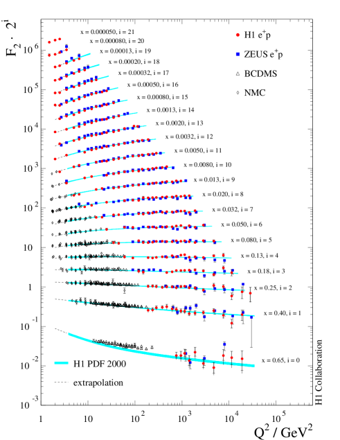
Figure 2.3: Measurements of the proton structure function $F_{2}(x_{B},Q^{2})$ from HERA collaborations and fixed target experiment. The data are shown as a function of $Q^{2}$ for various fixed values of $x_{B}$ (denoted as $x$ in the plot). Curves represent a NLO QCD fit to the data.

Figure 2.4: Comparison of two NLO QCD fits, corresponding to different input distributions [8], with the measurements of the proton structure function $F_{2}$ at small $x_{B}$ [62]. The results and data for the bins in $Q^{2}=1.5$ GeV² and 2 GeV² have been multiplied by 0.75 and 0.85, respectively, as indicated.

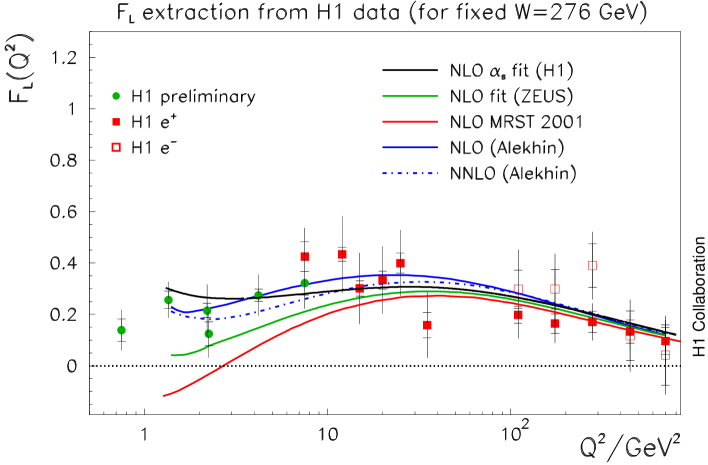
Figure 2.5: Measurements of the proton structure function $F_{L}$ by the H1 collaboration at HERA at a fixed value of $W=276$ GeV [65].

Figure 2.6: Measurements of the nucleon structure function $g_{1}$ as a function of $x_{B}$ (denoted as $x$ in the plot) at $Q^{2}=5$ GeV² [67]. The data are from the following experiments: E155 (solid circles), E143 (open circles), SMC (squares), HERMES (stars) and E154 (crosses). The solid curves correspond to a NLO QCD fit, while the dashed curves are from a purely phenomenological fit.

$$\frac{{\operatorname{d}}}{{\operatorname{d}}t}\left(\begin{array}[]{c}\Sigma(x_{B},Q^{2})\\ g(x_{B},Q^{2})\end{array}\right)=\hat{P}\otimes\left(\begin{array}[]{c}\Sigma\\ g\end{array}\right),$$ (2.100)

where $t=\ln Q^{2}/Q^{2}_{0}$ and the convolution ($\otimes$) is defined by

$$(P\otimes q)(x_{B},Q^{2})=\int_{x_{B}}^{1}\frac{{\operatorname{d}}y}{y}\,P\bigg{(}\frac{x_{B}}{y}\bigg{)}\,q(y,Q^{2}).$$ (2.101)

The splitting functions are given by

$$P_{\rm NS\,\pm}=\frac{\alpha_{s}(Q^{2})}{2\pi}\,P_{qq}^{(0)}(x_{B})+\bigg{(}\frac{\alpha_{s}(Q^{2})}{2\pi}\bigg{)}^{2}P^{(1)}_{{\rm NS\,\pm}}(x_{B})$$ (2.102)

and

$$\hat{P}=\frac{\alpha_{s}(Q^{2})}{2\pi}\,\hat{P}^{(0)}(x_{B})+\bigg{(}\frac{\alpha_{s}(Q^{2})}{2\pi}\bigg{)}^{2}\hat{P}^{(1)}(x_{B}),$$ (2.103)

where

$$\hat{P}^{(j)}(x_{B})=\left(\begin{array}[]{cc}P^{(j)}_{qq}&2n_{f}P^{(j)}_{qg}\\ P^{(j)}_{gq}&P^{(j)}_{gg}\end{array}\right),~{}~{}~{}~{}~{}~{}{\rm with}~{}~{}j=0,1;$$ (2.106)

$\alpha_{s}(Q^{2})$ being given in (2.92). The LO expressions are entailed in (2.92) and in (2.102)-(2.103); they can be obtained by simply dropping all higher order terms ($\beta_{1}$, $P^{(1)}$, $\hat{P}^{(1)}$). At LO (2.95), (2.100) reduce to the well-known DGLAP evolution equations [49, 50, 51, 52]. The complete set of NLO splitting functions in the commonly used $\overline{\rm MS}$ factorization scheme has been calculated [53, 54, 55] and can be found, for example, in [48].

Equations (2.95)-(2.103) hold also in the polarized sector, with the formal replacements $q\rightarrow\Delta q$ and $P\rightarrow\Delta P$. The polarized splitting functions are known up to NLO in the $\overline{\rm MS}$ scheme [56, 57, 58] and are listed in [59].

The resulting NLO parton distributions are directly related to physical quantities, such as structure functions, by a convolution with calculable, process dependent, coefficient functions. For consistency, the choice of the factorization convention must be the same for both the coefficient functions and the splitting functions underlying the parton distributions. Within the $\overline{\rm MS}$ scheme, $F_{2}(x_{B},Q^{2})$ is given by

$$\frac{1}{x_{B}}\,F_{2}(x_{B},Q^{2}) = \,\sum_{q}\,e^{2}_{q}\bigg{\{}q(x_{B},Q^{2})+\bar{q}(x_{B},Q^{2})$$ (2.107)

$$~{}~{}~{}~{}~{}~{}~{}+\frac{\alpha_{s}(Q^{2})}{2\pi}\,\bigg{[}C_{q}\otimes(q+\bar{q})+2C_{g}\otimes g\,\bigg{]}\bigg{\}},$$

where the unpolarized coefficients functions $C_{q,g}$ are given, for example, in [60] and in [61]. Measurements of the proton structure function $F_{2}$ together with a NLO QCD fit, presented in [62], are shown in Figure 2.3. As one can see, QCD appears to predict correctly the $Q^{2}$ dependence of structure function over four orders of magnitude.

Recently, a dedicated test of the validity of (2.107) at very low $x_{B}$ in the perturbative regime, $Q^{2}\gtrsim 1$ ${\rm GeV}^{2}$, has been performed [8] and the results are shown in Figure 2.4. A good agreement with recent precision data for $F_{2}$ [63], restricted to

$$3\times 10^{-5}\lesssim x_{B}\lesssim 3\times 10^{-3},~{}~{}~{}~{}~{}~{}~{}~{}~{}~{}1.5~{}{\rm GeV}^{2}\leq Q^{2}\leq 12~{}{\rm GeV}^{2},$$ (2.108)

has been found, as well as with the present experimental determination of the curvature of $F_{2}$ [64].

The structure function $F_{L}(x_{B},Q^{2})$ is only non-zero at order $\alpha_{s}$ in perturbation theory, i.e. $F_{L}(x_{B},Q^{2})={\cal{O}}(\alpha_{s})$; deviations from the Callan-Gross relation (2.85) are evident in Figure 2.5, taken from [65]. The data are much less precise than the ones for $F_{2}(x_{B},Q^{2})$, but QCD seems to work well also in this case.

Similarly to $F_{2}(x_{B},Q^{2})$, $g_{1}(x_{B},Q^{2})$ can be written as

$$g_{1}(x_{B},Q^{2}) = \frac{1}{2}\,\sum_{q}\,e^{2}_{q}\,\bigg{\{}\Delta q(x_{B},Q^{2})+\Delta\bar{q}(x_{B},Q^{2})$$ (2.109)

$$~{}~{}~{}~{}~{}~{}+\frac{\alpha_{s}(Q^{2})}{2\pi}\bigg{[}\Delta C_{q}\otimes(\Delta q+\Delta\bar{q})+2\Delta C_{g}\otimes\Delta g\bigg{]}\bigg{\}},$$

where $\Delta C_{q,g}$ can be found in [66]. In Figure 2.6 results on $g_{1}$ presented in [67] are shown as a function of $x_{B}$ at $Q^{2}=5$ ${\rm GeV}^{2}$.

At LO the coefficients $(\Delta)C_{q,g}$ vanish; from (2.107) and (2.109) it turns out that the gluon does not directly contribute to the structure functions, but only indirectly via the $Q^{2}$-evolution equations. The sums in (2.107) and in (2.109) usually run over the light quark-flavors $q=u$, $d$, $s$, since the heavy quark contributions ($c$, $b$, …) have preferrably to be calculated perturbatively from the intrisic light quarks ($u$, $d$, $s$) and gluon ($g$) partonic constituents of the nucleon. This treatment of the heavy quarks underlies the unpolarized GRV98 [68] and polarized GRSV01 [69] parton distributions, which will be used in our numerical estimates in the perturbative regime. For our studies in the low-$Q^{2}$ region, where perturbative QCD is not applicable, we resort to the purely phenomenological parametrization ALLM97 of $F_{2}$ [70] and to the parametrization BKZ of $g_{1}$ [71], shortly described in Chapters 5 and 7 respectively.

To conclude, it has been shown that the inclusion of ${\cal{O}(\alpha)}$ QED corrections to the parton evolution modifies only very slightly equations (2.95)-(2.100) [72, 73, 74], so we will not consider such effect. We will concentrate on the other consequence [73, 74] of the emission of photons from quarks, the appearence of the (inelastic) photon distributions of the proton and the neutron.

Chapter 3 The Equivalent Photon Distributions of the Nucleon

In this chapter the polarized and unpolarized photon content of protons and neutrons, evaluated in the equivalent photon approximation, are presented. In particular, the universal and process independent elastic photon components turn out to be uniquely determined by the well-known electromagnetic form factors of the nucleon and their derivation is shown in detail. The inelastic photon components are obtained from the corresponding momentum evolution equations subject to the boundary conditions of their vanishing at some low momentum scale. The resulting photon asymmetries, important for estimating cross section asymmetries in photon-induced subprocesses are also presented for some typical relevant momentum scales.

3.1 Unpolarized Photon Distributions

As already mentioned in the Introduction, the concept of the photon content of (charged) fermions is based on the EPA, the equivalent photon approximation. Applied to the nucleon $N=p,\,n$ it consists of two parts, an elastic one due to $N\to\gamma N$ and an inelastic part due to $N\to\gamma X$ with $X\neq N$. Accordingly the total photon distribution of the nucleon is given by

$$\gamma(x,\mu^{2})=\gamma_{\mathrm{el}}(x)+\gamma_{\mathrm{inel}}(x,\mu^{2}),$$ (3.1)

where $x$ is the fraction of the nucleon energy carried by the photon and $\mu$ is a momentum scale of the photon-induced subprocess. The two components are discussed separately in the following.

3.1.1 Elastic Component

The elastic photon distribution of the proton, $\gamma_{\mathrm{el}}^{p}$, has been presented in [24] and can be generally written as

$$\gamma_{\mathrm{el}}(x)=-\frac{\alpha}{2\pi}\int_{-\infty}^{-\frac{m^{2}x^{2}}{1-x}}\frac{{\operatorname{d}}t}{t}\left\{\left[2\left(\frac{1}{x}-1\right)+\frac{2m^{2}x}{t}\right]H_{1}(t)+xG_{M}^{2}(t)\right\},$$ (3.2)

where

$$H_{1}(t)\equiv F_{1}^{2}(t)+\tau F_{2}^{2}(t)=\frac{G_{E}^{2}(t)+\tau G_{M}^{2}(t)}{1+\tau}$$ (3.3)

with $\tau\equiv-t/4m^{2}$, $m$ being the nucleon mass, and where $G_{E}$ and $G_{M}$ are the Sachs elastic form factors discussed in Section 2.1.

The result (3.2) can be obtained extending to an unpolarized nucleon $N$ the analysis [21] for a photon emitting unpolarized electron. We consider the process

$$N(P)+a(l)\rightarrow N(P^{\prime})+X,$$ (3.4)

where the target $a$ is a massless parton ($l^{2}=0$), $P^{2}=P^{\prime 2}=m^{2}$, and $X$ is a generic hadronic system. The corresponding cross section can be written as

$${\operatorname{d}}\sigma_{Na}(P,l)=\frac{1}{4P\cdot l}\,\frac{1}{q^{4}}\,H_{\mathrm{el}}^{\alpha\beta}(P;P^{\prime})W_{\alpha\beta}(k,l)\,\frac{{\operatorname{d}}^{3}{\mbox{\boldmath$P$}}^{\prime}}{(2\pi)^{3}2E^{\prime}}~{},$$ (3.5)

where

$$q\equiv-k=P^{\prime}-P,$$ (3.6)

$k$ being the four-momentum of photon emitted by the nucleon. The tensor $H_{\mathrm{el}}^{\alpha\beta}(P;P^{\prime})$ is defined in (2.18) and, using (2.24), (3.3) and (3.6), can be rewritten in a more compact form as

$$H^{\alpha\beta}_{\mathrm{el}}(P;P^{\prime})=e^{2}\,[H_{1}(q^{2})(2P-k)^{\alpha}(2P-k)^{\beta}+G_{M}^{2}(q^{2})(q^{2}g^{\alpha\beta}-k^{\alpha}k^{\beta})].$$ (3.7)

The partonic tensor $W_{\alpha\beta}(k,l)$, as shown in (2.45), can be decomposed as

$$W_{\alpha\beta}(k,l) = 4\pi e^{2}\bigg{[}\bigg{(}-g_{\alpha\beta}+\frac{1}{q^{2}}\,k_{\alpha}k_{\beta}\bigg{)}F_{1}(q^{2},k\cdot l)$$ (3.8)

$$-\frac{1}{(k\cdot l)}\,\bigg{(}l_{\alpha}-\frac{k\cdot l}{q^{2}}\,k_{\alpha}\bigg{)}\bigg{(}l_{\beta}-\frac{k\cdot l}{q^{2}}\,k_{\beta}\bigg{)}F_{2}(q^{2},k\cdot l)\bigg{]},$$

with the structure functions $F_{1}$ and $F_{2}$ defined in (2.50) and (2.51). As pointed out in [21], in the limit $q^{2}\rightarrow 0$, $W_{\alpha\beta}(k,l)$ must be an analytic function of $q^{2}$, therefore $q^{2}W_{\alpha\beta}$ has to vanish for $q^{2}=0$. This implies

$$\frac{(k\cdot l)}{q^{2}}\,F_{2}(q^{2},k\cdot l)=F_{1}(0,k\cdot l)+{\cal{O}}(q^{2}),$$ (3.9)

and the terms ${\cal{O}}(q^{2})$ will not be considered in the following. Furthermore, one can introduce the variable

$$x=\frac{k\cdot l}{P\cdot l}~{},$$ (3.10)

which represents the fraction of longitudinal momentum carried by the emitted photon, assumed to be real and collinear with the parent nucleon, that is

$$k=xP.$$ (3.11)

From (3.7)-(3.10) one finds

$$H_{\mathrm{el}}^{\alpha\beta}(P;P^{\prime})W_{\alpha\beta}(k,l)=4\pi e^{4}\bigg{\{}4H_{1}(q^{2})\bigg{[}-m^{2}+\frac{q^{2}}{x}-\frac{q^{2}}{x^{2}}\bigg{]}-2q^{2}G_{M}^{2}(q^{2})\bigg{\}}F_{1}(0,l\cdot k).$$

If we write the four-momenta of the incoming and outgoing nucleons as

$$P=(E,0,0,E\beta),~{}~{}~{}~{}~{}~{}~{}P^{\prime}=(E^{\prime},0,E^{\prime}\beta^{\prime}\sin\theta,E^{\prime}\beta^{\prime}\cos\theta),$$ (3.13)

with

$$\beta=\sqrt{1-\frac{m^{2}}{E^{2}}}~{},~{}~{}~{}~{}~{}~{}~{}~{}~{}~{}~{}\beta^{\prime}=\sqrt{1-\frac{m^{2}}{E^{\prime 2}}}~{},$$ (3.14)

then the phase space for the scattered nucleon will be given by

$$\frac{{\operatorname{d}}^{3}{\mbox{\boldmath$P$}}^{\prime}}{E^{\prime}}=2\pi\beta^{\prime 2}E^{\prime}{\operatorname{d}}P^{\prime}{\operatorname{d}}\cos\theta,$$ (3.15)

where the azimuth integration has already been carried out. The integration variables ($P^{\prime}$, $\cos\theta$) can be replaced by ($q^{2}$, $x$); using the following relations

$$q^{2} = 2m^{2}-2EE^{\prime}(1-\beta\beta^{\prime}\cos\theta),$$ (3.16)

$$x = 1-\frac{E^{\prime}(1+\beta^{\prime}\cos\theta)}{E(1+\beta)}~{},$$ (3.17)

it can be proved that the Jacobian of this change of variables is $2E^{\prime}\beta^{\prime 2}$ and (3.15) becomes

$$\frac{{\operatorname{d}}^{3}{\mbox{\boldmath$P$}}^{\prime}}{E^{\prime}}=\pi{\operatorname{d}}q^{2}{\operatorname{d}}x.$$ (3.18)

The cross section (3.5) can now be written as

$${\operatorname{d}}\sigma_{Na}(P,l)=-\frac{\alpha}{2\pi}\,\frac{1}{t}\bigg{\{}\bigg{[}\frac{2m^{2}x}{t}+2\bigg{(}\frac{1}{x}-1\bigg{)}\bigg{]}\,H_{1}(t)+xG_{M}^{2}(t)\bigg{\}}\,\sigma_{\gamma a}(k,l)\,{\operatorname{d}}t\,{\operatorname{d}}x,$$ (3.19)

where $t\equiv q^{2}$ and

$$\sigma_{\gamma a}(k,l)=-\frac{1}{8\,k\cdot l}\,g_{\alpha\beta}W^{\alpha\beta}(k,l)=\frac{\pi e^{2}}{\,k\cdot l}\,F_{1}(0,k\cdot l)$$ (3.20)

is the cross section for the process $\gamma(k)+N(P)\rightarrow X$ for a real photon. Integrating over $t$ one gets

$${\operatorname{d}}\sigma_{Na}(P,l)=\gamma_{\mathrm{el}}(x)\,\sigma_{\gamma a}(k,l)\,{\operatorname{d}}x,$$ (3.21)

where $\gamma_{\mathrm{el}}(x)$ is given by

$$\gamma_{\mathrm{el}}(x)=-\frac{\alpha}{2\pi}\int_{t_{\mathrm{min}}}^{t_{\mathrm{max}}}\frac{{\operatorname{d}}t}{t}\left\{\left[2\left(\frac{1}{x}-1\right)+\frac{2m^{2}x}{t}\right]H_{1}(t)+xG_{M}^{2}(t)\right\}.$$ (3.22)

The extrema of integration can be determined from (3.16) and (3.17); from the latter we have

$$E^{\prime}=\frac{A}{1-\cos^{2}\theta}\,\bigg{(}1-\sqrt{1-\frac{(A^{2}+m^{2}\cos^{2}\theta)(1-\cos^{2}\theta)}{A^{2}}}~{}\bigg{)},$$ (3.23)

where

$$A=E(1+\beta)(1-x).$$ (3.24)

Expanding (3.23) in powers of $\theta$, for $\theta\ll 1$, one gets [21]

$$E^{\prime}=\frac{A^{2}+m^{2}}{2A}+\frac{(A^{2}-m^{2})^{2}}{8A^{3}}\,\theta^{2}+{\cal{O}}(\theta^{4}),$$ (3.25)

and (3.16) becomes

$$q^{2}=-\frac{m^{2}x^{2}}{1-x}-\frac{E(1+\beta)(A^{2}-m^{2})^{2}}{4A^{3}}\,\theta^{2}+{\cal{O}}(\theta^{4}).$$ (3.26)

The value $t_{\mathrm{max}}=q^{2}_{\mathrm{max}}$ is obtained by taking $\theta=0$, namely

$$t_{\mathrm{max}}=-\frac{m^{2}x^{2}}{1-x}~{}.$$ (3.27)

The minimum value of the photon virtuality $t_{\mathrm{min}}$ can be computed in a simple way by imposing that the invariant mass $W^{2}$ of the produced hadronic system $X$ be bounded from below [21]:

$$W^{2}\equiv(k+l)^{2}>W^{2}_{\mathrm{min}},$$ (3.28)

from which it comes, for $W^{2}_{\mathrm{min}}=m^{2}$,

$$t_{\mathrm{min}}=-2k\cdot l+m^{2}=-2xP\cdot l+m^{2}=-x(s-m^{2})+m^{2},$$ (3.29)

where $s$ is the nucleon-parton centre-of-mass energy squared.

The Sachs form factors which appear in (3.22) are conveniently parametrized by the dipole form proportional to $(1-t/0.71$ GeV${}^{2})^{-2}$ as extracted from experiment, see (2.28). As pointed out in [24], this implies that the support from values $t\ll-0.71$ $\mathrm{GeV}^{2}$ to the integral in (3.22) is suppressed, hence, in the kinematical region $xs\gg m^{2}$, one may integrate from $t_{\mathrm{min}}=-\infty$ to $t_{\max}=-m^{2}x^{2}/(1-x)$ so as to obtain the universal process independent $\gamma_{\mathrm{el}}$ in (3.2) .

Equation (3.2) can now be analytically integrated, remembering that, from (2.28) and (3.3), for the proton we have

$$G_{E}^{p}(t)=(1+a\tau)^{-2}\,,\quad\quad G_{M}^{p}(t)\simeq\mu_{p}G_{E}^{p}(t)\,,\quad\quad H_{1}^{p}(t)=\frac{1+\mu_{p}^{2}\tau}{1+\tau}(1+a\tau)^{-4}$$ (3.30)

with $\mu_{p}=1+\kappa_{p}\simeq 2.79$ and $a\equiv 4m^{2}/0.71$ GeV${}^{2}\simeq 4.96$, while for the neutron

$$G_{E}^{n}(t)=\kappa_{n}\tau(1+a\tau)^{-2}\,,\quad\quad G_{M}^{n}(t)=\kappa_{n}(1+a\tau)^{-2}\,,\quad\quad H_{1}^{n}(t)=\kappa_{n}^{2}\tau(1+a\tau)^{-4}\,,$$ (3.31)

with $\kappa_{n}\simeq-1.79$. After integration, the elastic component of the equivalent photon distribution reads [1], for the proton

$$\gamma_{\mathrm{el}}^{p}(x) = \frac{\alpha}{2\pi}\,\frac{2}{x}\left\{\left[1-x+\frac{x^{2}}{4}(1+4a+\mu_{p}^{2})\right]I+(\mu_{p}^{2}-1)\left[1-x+\frac{x^{2}}{4}\right]\tilde{I}-\frac{1-x}{z^{3}}\right\},$$

and for the neutron

$$\gamma_{\mathrm{el}}^{n}(x)=\frac{\alpha}{2\pi}\,\kappa_{n}^{2}\frac{x}{2}\left\{I+\frac{1}{3}\,\frac{1}{(z-1)z^{3}}\right\},$$ (3.33)

where $z\equiv 1+\frac{a}{4}\,\frac{x^{2}}{1-x}$ and

$$I = \int_{\frac{x^{2}}{4(1-x)}}^{\infty}{\operatorname{d}}\tau\frac{1}{\tau(1+a\tau)^{4}}=-\ln\left(1-\frac{1}{z}\right)-\frac{1}{z}-\frac{1}{2z^{2}}-\frac{1}{3z^{3}}~{},$$ (3.34)

$$\tilde{I} = \int_{\frac{x^{2}}{4(1-x)}}^{\infty}{\operatorname{d}}\tau\frac{1}{(1+\tau)(1+a\tau)^{4}}=-\frac{1}{a_{-}^{4}}\ln\left(1+\frac{a_{-}}{z}\right)+\frac{1}{a_{-}^{3}z}-\frac{1}{2a_{-}^{2}z^{2}}+\frac{1}{3a_{-}z^{3}}~{},$$

with $a_{-}=a-1$. For arriving at (LABEL:eqsix) we have utilized the relation

$$\int_{\frac{x^{2}}{4(1-x)}}^{\infty}{\operatorname{d}}\tau\frac{1}{\tau^{2}(1+a\tau)^{4}}=-4aI+4\frac{1-x}{x^{2}z^{3}}~{},$$

which will be also relevant for the polarized photon contents to be presented below. The result in (LABEL:eqsix) agrees with the one presented in a somewhat different form in [24].

If we integrate (3.21) taking $G_{E}^{2}=G_{M}^{2}=1$ (pointlike particle), with the integration bounds (3.27) and $t_{\rm min}\equiv-\mu^{2}$, we recover the result (1.4) for the unpolarized photon content of the electron.

3.1.2 Inelastic Component

As pointed out in [27], the complete function $\gamma(x,\mu^{2})$ in (3.1) could be built-up by adding to the elastic contribution all resonant [34] and non-resonant final hadronic states, and their interferences. Alternatively one could guess an inclusive or ’continuous’ $\gamma_{\mathrm{inel}}(x,\mu^{2})$, based on the parton model, where the photon is emitted by one of the quarks in the nucleon [25]. In this latter picture, which we adopt, the addition of the resonant and continuous contributions may be double-counting. The inelastic part in (3.1) is then given by the leading order (LO) QED evolution equation [25]

$$\frac{{\operatorname{d}}\gamma_{\mathrm{inel}}(x,\mu^{2})}{{\operatorname{d}}\ln\mu^{2}}=\frac{\alpha}{2\pi}\sum_{q=u,d,s}e_{q}^{2}\int_{x}^{1}\frac{dy}{y}\,P_{\gamma q}\left(\frac{x}{y}\right)\left[q(y,\mu^{2})+\bar{q}(y,\mu^{2})\right],$$ (3.36)

where

$$P_{\gamma q}(y)=\frac{1+(1-y)^{2}}{y}$$ (3.37)

is the quark-to-photon splitting function and $q(y,\mu^{2})$, $\bar{q}(y,\mu^{2})$ are respectively the quark and antiquark distribution functions of the nucleon at LO QCD [68], with $\stackrel{{\scriptstyle\!\!\!(-)}}{{u^{p}}}=\stackrel{{\scriptstyle\,(-)}}{{d^{n}}}$, $\stackrel{{\scriptstyle\!\!\!(-)}}{{d^{p}}}=\stackrel{{\scriptstyle\!\!\!(-)}}{{u^{n}}}$, $\stackrel{{\scriptstyle\!\!\!(-)}}{{s^{p}}}=\stackrel{{\scriptstyle(-)}}{{s^{n}}}$. Equation (3.36), which states that the probability to find a photon in the nucleon is given by the convolution of the probabilities to find first a quark inside the nucleon and then a photon inside the quark, is integrated subject to the ‘minimal’ boundary condition

$$\gamma_{\mathrm{inel}}(x,\mu_{0}^{2})=0$$ (3.38)

at [68] $\mu_{0}^{2}=0.26$ GeV². The boundary condition (3.38) is obviously not compelling and affords further theoretical and experimental studies. Since for the time being there are no experimental measurements available, the ‘minimal’ boundary condition provides at present a rough estimate for the inelastic component at $\mu^{2}\gg\mu_{0}^{2}$.

3.2 Polarized Photon Distributions

The previous analysis can be extended to the polarized sector, i.e., to

$$\Delta\gamma(x,\mu^{2})=\Delta\gamma_{\mathrm{el}}(x)+\Delta\gamma_{\mathrm{inel}}(x,\mu^{2})\,.$$ (3.39)

As before, the elastic and inelastic parts will be studied separately.

3.2.1 Elastic Component

The elastic part $\Delta\gamma_{\mathrm{el}}(x)$ in (3.39) is determined via the antisymmetric part of the tensor describing the photon emitting nucleon $N$

$$H_{\mathrm{el}}^{\alpha\beta}(P;P^{\prime})=\frac{1}{2}\,e^{2}\,\mathrm{Tr}\left[(1+\gamma^{5}S\!\!\!/)(P\!\!\!\!/+m)\Gamma^{\alpha}(P\!\!\!\!/\,^{\prime}+m)\Gamma^{\beta}\right]$$ (3.40)

for the process

$$N(P;\,S)+a(l;\,s)\to N({P^{\prime}})+X$$ (3.41)

where $a$ being a parton with four-momentum $l$ initially kept off-shell and $S$, $s$ are the polarization vectors [22] satisfying the transversality condition $S\cdot P=0$ and $s\cdot l=0$. Equation tensor has been obtained in a way similar to (2.61), with $\gamma^{\alpha}\to\Gamma^{\alpha}$. In terms of the Dirac and Pauli form factors $F_{1,2}(t)$ the elastic vertices $\Gamma^{\alpha}$ are given by

$$\Gamma^{\alpha}=(F_{1}+F_{2})\gamma^{\alpha}-\frac{1}{2m}F_{2}(P+{P^{\prime}})^{\alpha}\,.$$ (3.42)

The analysis has been carried out originally in [1] and is a straightforward extension of the calculation [22] of the polarized equivalent photon distribution resulting from a photon emitting electron. The antisymmetric part of (3.40), as calculated in [1], reads

$$H_{\mathrm{el}}^{\alpha\beta{\rm A}}(P;P^{\prime}) = 2ie^{2}m\,G_{M}^{2}\,\varepsilon^{\alpha\beta\rho\sigma}S_{\rho}k_{\sigma}+2i\,G_{M}(F_{2}/2m)$$ (3.43)

$$~{}~{}~{}\times\,\left[(P+{P^{\prime}})^{\alpha}\,\varepsilon^{\beta\rho\sigma\sigma^{\prime}}-(P+{P^{\prime}})^{\beta}\varepsilon^{\alpha\rho\sigma\sigma^{\prime}}\right]S_{\rho}P_{\sigma}{P^{\prime}}_{\sigma^{\prime}}$$

with, as before, $k=P-{P^{\prime}}$. One can show that

$$\left[(P+P^{\prime})^{\alpha}\varepsilon^{\beta\rho\sigma\sigma^{\prime}}-(P+P^{\prime})^{\beta}\varepsilon^{\alpha\rho\sigma\sigma^{\prime}}\right]S_{\rho}P_{\sigma}P^{\prime}_{\sigma^{\prime}} = (k\cdot S)P_{\sigma}k_{\sigma^{\prime}}\varepsilon^{\beta\alpha\sigma\sigma^{\prime}}~{}~{}~{}~{}~{}~{}~{}~{}~{}~{}~{}~{}~{}~{}~{}~{}~{}~{}~{}~{}$$ (3.44)

$$+\,\,(2m^{2}+P\cdot k)\varepsilon^{\beta\rho\alpha\sigma^{\prime}}S_{\rho}k_{\sigma^{\prime}},$$

where we made use of the $\varepsilon$-identity

$$g^{\alpha\mu}\varepsilon^{\beta\rho\sigma\sigma^{\prime}}=g^{\alpha\beta}\varepsilon^{\mu\rho\sigma\sigma^{\prime}}+g^{\alpha\rho}\varepsilon^{\beta\mu\sigma\sigma^{\prime}}+g^{\alpha\sigma}\varepsilon^{\beta\rho\mu\sigma^{\prime}}+g^{\alpha\sigma^{\prime}}\varepsilon^{\beta\rho\sigma\mu};$$ (3.45)

hence (3.43) can be rewritten in a more compact form [75] as

$$H^{\alpha\beta{\rm A}}_{\mathrm{el}}(P;P^{\prime})=-ie^{2}m\varepsilon^{\alpha\beta\rho\sigma}k_{\rho}\bigg{[}2G_{E}G_{M}S_{\sigma}-{G_{M}(G_{M}-G_{E})\over 1+\tau}{k\cdot S\over m^{2}}P_{\sigma}\bigg{]}.$$ (3.46)

The polarized cross section relative to the process (3.41) is given by

$${\operatorname{d}}\Delta\sigma_{Na}(P,l)=\frac{1}{4\,P\cdot l}\,\frac{1}{q^{4}}\,H_{\mathrm{el}}^{\alpha\beta{\rm A}}(P;P^{\prime})\,W_{\alpha\beta}^{\rm A}(k,l)\,\frac{{\operatorname{d}}^{3}{\mbox{\boldmath$P$}}^{\prime}}{(2\pi)^{3}2E^{\prime}}~{},$$ (3.47)

where $W_{A}^{\alpha\beta}$ is the antisymmetric part of the partonic tensor, describing the polarized target $a(l;\,s)$, which is expressed in terms of the usual polarized structure functions $g_{1}$ and $g_{2}$, see (2.57) together with (2.69) and (2.70),

$$W^{\rm A}_{\alpha\beta}(k,l)=2i\pi e^{2}\frac{\sqrt{|l^{2}|}}{k\cdot l}\,\varepsilon_{\alpha\beta\rho\sigma}k^{\rho}\bigg{[}g_{1}(q^{2},k\cdot l)s^{\sigma}+g_{2}(q^{2},k\cdot l)\bigg{(}s^{\sigma}-{k\cdot s\over k\cdot l}\,l^{\sigma}\bigg{)}\bigg{]}.$$ (3.48)

The spin vectors for the incoming nucleon and parton can be written as

$$S_{\alpha}=N_{S}\bigg{(}P_{\alpha}-\frac{m^{2}}{l\cdot P}\,l_{\alpha}\bigg{)},~{}~{}~{}~{}~{}s_{\alpha}=N_{s}\bigg{(}l_{\alpha}-\frac{l^{2}}{l\cdot P}\,P_{\alpha}\bigg{)},$$ (3.49)

where the normalization factors $N_{S}$ and $N_{s}$ are related to $S^{2}$ and $s^{2}$ by [76]

$$N^{2}_{S}=-\frac{S^{2}}{m^{2}\tilde{\beta}^{2}}\,,~{}~{}~{}N^{2}_{s}=-\frac{s^{2}}{l^{2}\tilde{\beta}^{2}}\,,$$ (3.50)

with

$$\tilde{\beta}=\sqrt{1-\frac{m^{2}l^{2}}{(P\cdot l)^{2}}}\,,$$ (3.51)

and are fixed in order to satisfy the condition $|S^{2}|=|s^{2}|=1$.
Putting the parton on-shell ($l^{2}=0$) and using the definition (3.10), together with (3.49), we have

$$H_{\mathrm{el}}^{\alpha\beta{\rm A}}(P;P^{\prime})W^{\rm A}_{\alpha\beta}(k,l) = -4\pi e^{4}q^{2}\bigg{\{}\bigg{[}\frac{2m^{2}x}{q^{2}}-1+\frac{2}{x}\bigg{]}\,G_{M}^{2}~{}~{}~{}~{}~{}~{}~{}~{}~{}~{}~{}~{}~{}~{}~{}~{}~{}~{}~{}~{}~{}~{}~{}~{}~{}~{}~{}~{}~{}~{}~{}~{}~{}~{}$$ (3.52)

$$~{}~{}~{}-2\bigg{[}\frac{m^{2}x}{q^{2}}-1+\frac{1}{x}\bigg{]}\frac{G_{M}(G_{M}-G_{E})}{1+\tau}\bigg{\}}\,g_{1}(q^{2},k\cdot l),$$

where all the terms proportional to $g_{2}$ drop from this equation. Then (3.47) becomes

$${\operatorname{d}}\Delta\sigma_{Na}(P,l) = -\frac{\alpha}{2\pi}\,\frac{1}{q^{2}}\bigg{\{}\bigg{[}1+\frac{2m^{2}x}{q^{2}}-\frac{2}{x}\bigg{]}\,G_{M}^{2}$$ (3.53)

$$~{}~{}~{}-2\bigg{[}1+\frac{m^{2}x}{q^{2}}-\frac{1}{x}\bigg{]}\frac{G_{M}(G_{M}-G_{E})}{1+\tau}\bigg{\}}\,2\pi^{2}\alpha\,\frac{g_{1}(0,k\cdot l)}{P\cdot l}~{},$$

which holds in the limit $q^{2}\rightarrow 0$, after changing the variables of integration as for the unpolarized case. This expression can be related to the polarized cross section for real photon-parton scattering, which can be computed by convoluting the partonic tensor with the antisymmetric part of the photon polarization density matrix [76]

$$P^{\rm A}_{\alpha\beta}=\frac{1}{2}\,(\,\epsilon_{\alpha}\epsilon_{\beta}^{*}-\epsilon_{\beta}\epsilon_{\alpha}^{*})=\frac{i}{2\sqrt{|q^{2}|}}\,\varepsilon_{\alpha\beta\rho\sigma}k^{\rho}t^{\sigma},$$ (3.54)

where $\epsilon^{\mu}$ is the photon polarization vector and $t^{\alpha}$ is its spin vector

$$t_{\alpha}=N_{t}\,\bigg{(}k_{\alpha}-\frac{q^{2}}{k\cdot l}\,l_{\alpha}\bigg{)},$$ (3.55)

with $N_{t}$ chosen so that $|t^{2}|=1$. We get ($q^{2}\rightarrow 0$)

$$\Delta\sigma_{\gamma a}(k,l)=\frac{1}{4\,k\cdot l}\,W^{\alpha\beta{\rm A}}P^{\rm A}_{\alpha\beta}=2\pi^{2}\alpha\,\frac{g_{1}(0,k\cdot l)}{k\cdot l}~{}.$$ (3.56)

Combining the last equation with (3.53) and integrating over $q^{2}$, one gets the analogous of (3.21) for a polarized process

$${\operatorname{d}}\Delta\sigma_{Na}(P,l)=\Delta\gamma_{\mathrm{el}}(x)\Delta\sigma_{\gamma a}(k,l){\operatorname{d}}x,$$ (3.57)

with [1]

$$\Delta\gamma_{\mathrm{el}}(x) = -\frac{\alpha}{2\pi}\int_{t_{\rm min}}^{t_{\rm max}}\frac{{\operatorname{d}}t}{t}\left\{\left[2-x+\frac{2m^{2}x^{2}}{t}\right]G_{M}^{2}(t)-2\left[1-x+\frac{m^{2}x^{2}}{t}\right]G_{M}(t)F_{2}(t)\right\}$$ (3.58)

$$= -\frac{\alpha}{2\pi}\int_{t_{\rm min}}^{t_{\rm max}}\frac{{\operatorname{d}}t}{t}\,G_{M}(t)\left\{\left[2-x+\frac{2m^{2}x^{2}}{t}\right]F_{1}(t)+xF_{2}(t)\right\}$$

where the first term proportional to $G_{M}^{2}$ in the first line corresponds to the pointlike result of [22]. Following [24], we again approximate the integration bounds by $t_{\rm min}=-\infty$ and $t_{\rm max}=-m^{2}x^{2}/(1-x)$ as in (3.2) in order to obtain an universal process independent polarized elastic distribution. Using, in addition to (3.30) and (3.31),

$$F_{1}^{p}(t) = \frac{1+\mu_{p}\tau}{1+\tau}\,(1+a\tau)^{-2},\quad F_{2}^{p}(t)=\frac{\kappa_{p}}{1+\tau}(1+a\tau)^{-2}$$ (3.59)

$$F_{1}^{n}(t) = 2\kappa_{n}\frac{\tau}{1+\tau}(1+a\tau)^{-2},\quad F_{2}^{n}(t)=\kappa_{n}\frac{1-\tau}{1+\tau}(1+a\tau)^{-2}\,,$$ (3.60)

equation (3.58) yields for the proton

$$\Delta\gamma_{\mathrm{el}}^{p}(x)=\frac{\alpha}{2\pi}\,\mu_{p}\left\{\left[(2-x)\left(1+\kappa_{p}\frac{x}{2}\right)+2ax^{2}\right]I+2\kappa_{p}\left(1-x+\frac{x^{2}}{4}\right)\tilde{I}-2\,\frac{1-x}{z^{3}}\right\}\,,$$ (3.61)

and for the neutron

$$\Delta\gamma_{\mathrm{el}}^{n}(x)=\frac{\alpha}{2\pi}\kappa_{n}^{2}\left\{x(1-x)I+4\left(1-x+\frac{x^{2}}{4}\right)\tilde{I}\right\}$$ (3.62)

with $I$ and $\tilde{I}$ being given in ( 3.34) and (3.1.1).

Integrating (3.58) between $t_{\rm min}=-\mu^{2}$ and $t_{\rm max}$ given in (3.27), with the form factors $G_{M}=F_{1}=-1$ and $F_{2}=0$, we obtain the polarized photon distribution of the electron (1.10).

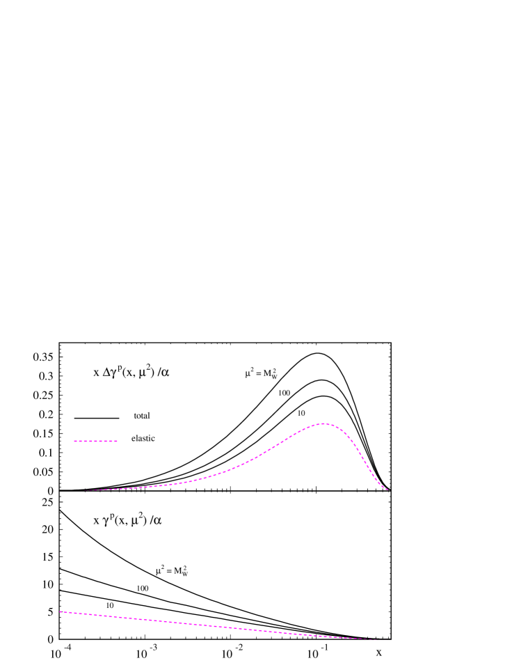
Figure 3.1: The polarized and unpolarized total photon contents of the proton, $\Delta\gamma^{p}$ and $\gamma^{p}$, according to (3.1) and (3.39) at some typical fixed values of $\mu^{2}$ (in GeV²). The $\mu^{2}$-independent elastic contributions are given by (3.61) and (LABEL:eqsix).

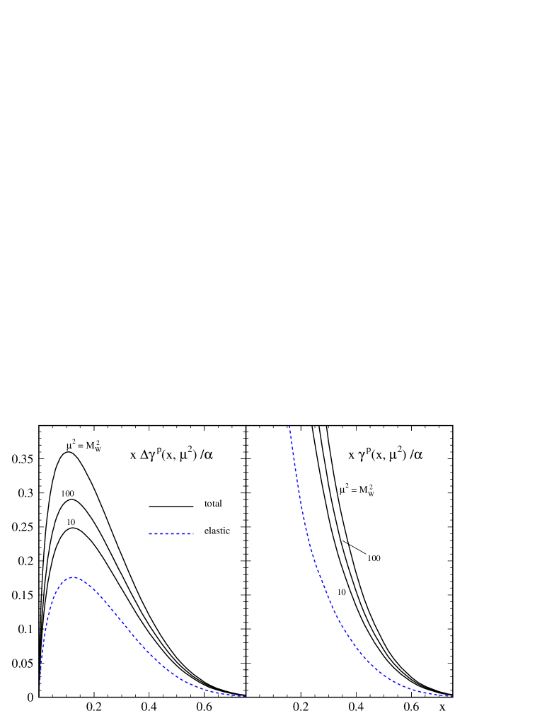
Figure 3.2: As in Figure 3.1 but for a linear $x$ scale.

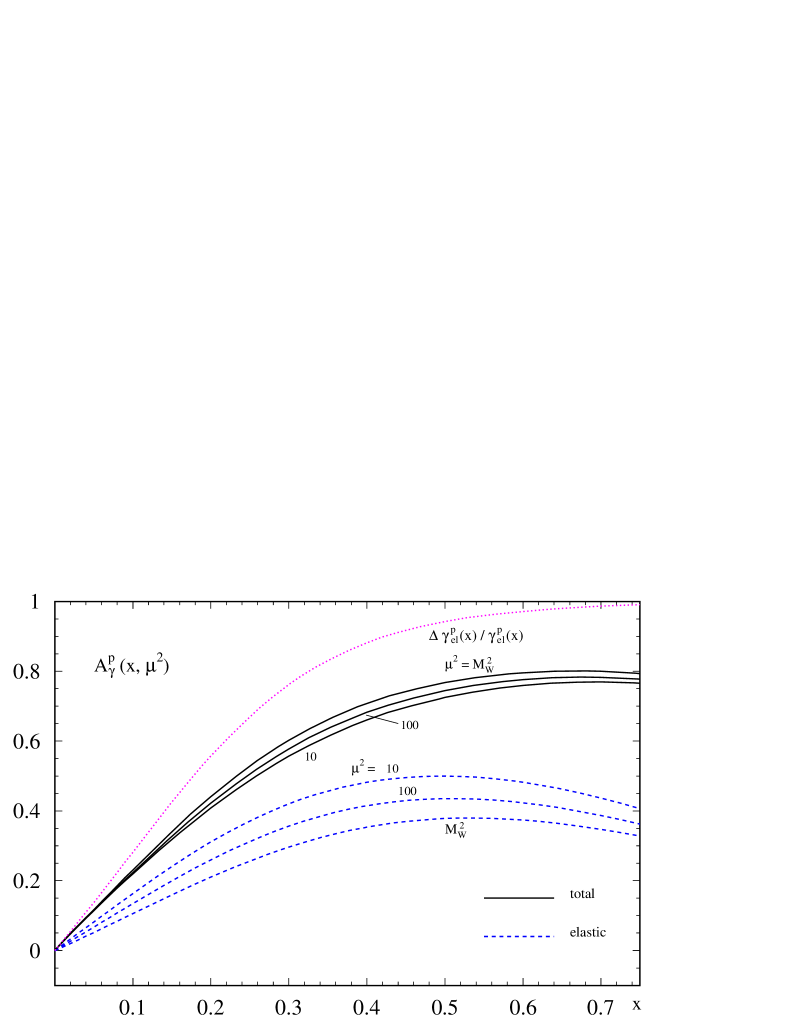
Figure 3.3: The asymmetry of the polarized to the unpolarized photon content of the proton as defined in (3.66) at various fixed values of $\mu^{2}$ (in GeV²) according to the results in Figure 3.1. The $\mu^{2}$-dependence of the elastic contribution to $A_{\gamma}^{p}$ is caused by the $\mu^{2}$-dependent total unpolarized photon content in the denominator of (3.66). For illustration the $\mu^{2}$-independent elastic ratio $\Delta\gamma_{\mathrm{el}}^{p}/\gamma_{\mathrm{el}}^{p}$ is shown as well.

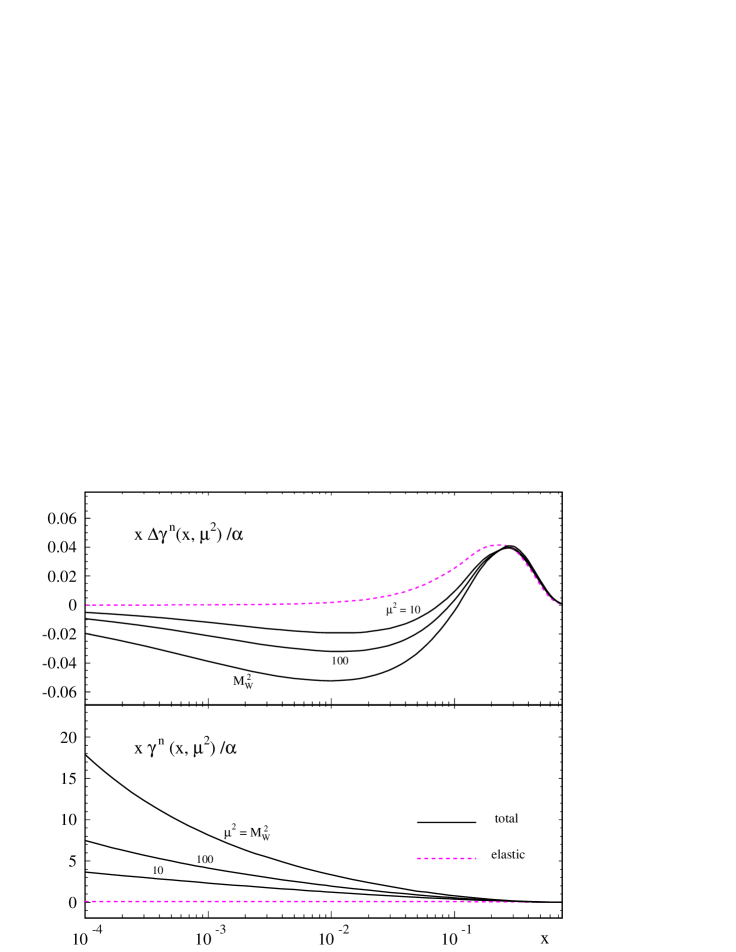
Figure 3.4: As Figure 3.1 but for the neutron, with elastic polarized and unpolarized contributions being given by (3.62) and (3.33).

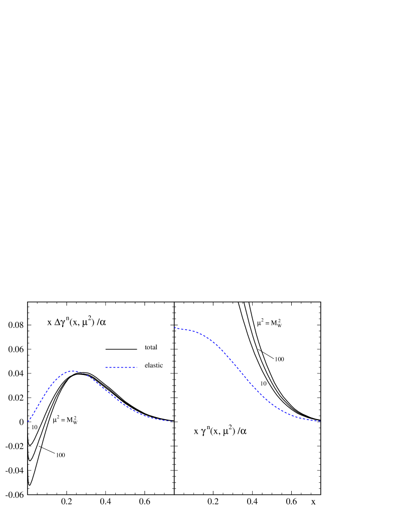
Figure 3.5: As in Figure 3.4 but for a linear $x$ scale.

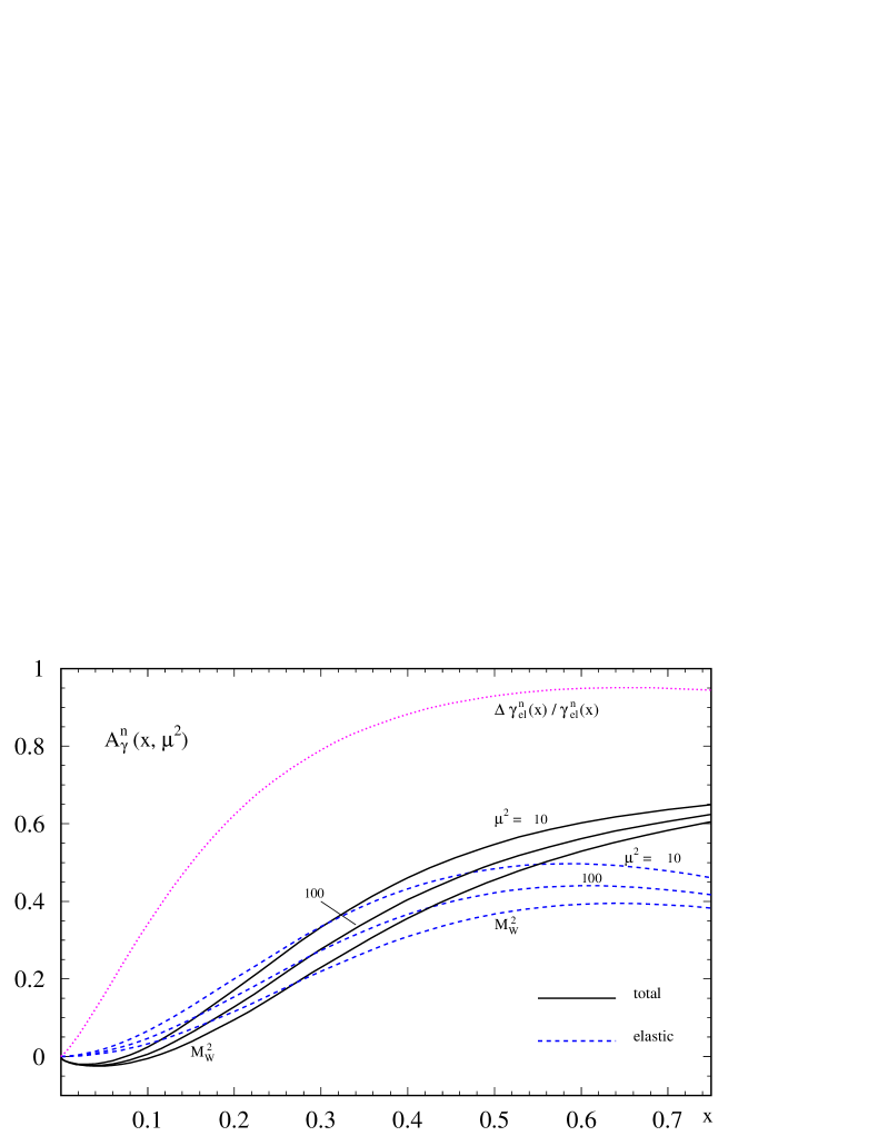
Figure 3.6: As Figure 3.3 but for the neutron asymmetry according to the results in Figure 3.4.

3.2.2 Inelastic Component

The inelastic contribution [1] derives from a straightforward extension of (3.36),

$$\frac{{\operatorname{d}}\Delta\gamma_{\mathrm{inel}}(x,\mu^{2})}{{\operatorname{d}}\ln\mu^{2}}=\frac{\alpha}{2\pi}\sum_{q=u,d,s}e_{q}^{2}\int_{x}^{1}\,\frac{{\operatorname{d}}y}{y}\,\Delta P_{\gamma q}\left(\frac{x}{y}\right)\left[\Delta q(y,\mu^{2})+\Delta\bar{q}(y,\mu^{2})\right]$$ (3.63)

where

$$\Delta P_{\gamma q}(y)=\frac{1-(1-y)^{2}}{y}=2-y$$ (3.64)

is the polarized quark-to-photon splitting function and $\Delta q(y,\mu^{2})$, $\Delta\bar{q}(y,\mu^{2})$ are the polarized quark and antiquark distribution functions of the nucleon. We integrate this evolution equation assuming again the not necessarily compelling ‘minimal’ boundary condition

$$\Delta\gamma_{\mathrm{inel}}(x,\mu_{0}^{2})=0,$$ (3.65)

according to $|\Delta\gamma_{\mathrm{inel}}(x,\mu_{0}^{2})|\leq\gamma_{\mathrm{inel}}(x,\mu_{0}^{2})=0$, at $\mu_{0}^{2}=0.26$ GeV² using the LO polarized parton densities of [69]. These latter two equations together with (3.63) yield now the total photon content $\Delta\gamma(x,\mu^{2})$ of a polarized nucleon in (3.39).

3.3 Numerical Results

Our results for $\Delta\gamma^{p}(x,\mu^{2})$ in (3.39) are shown in Figure 3.1 for some typical values of $\mu^{2}$ up to $\mu^{2}=M_{W}^{2}=6467$ GeV². For comparison the expectations for the unpolarized $\gamma^{p}(x,\mu^{2})$ in (3.1) are depicted as well. The $\mu^{2}$-independent polarized and unpolarized elastic contributions in (3.61) and (LABEL:eqsix), respectively, are also shown separately. Due to the singular small-$y$ behavior of the unpolarized parton distributions $y\!\!\stackrel{{\scriptstyle(-)}}{{q}}\!\!(y,\mu^{2})$ in (3.36) as well as of the singular $x\gamma_{\mathrm{el}}^{p}(x)$ in (LABEL:eqsix) as $x\to 0$, the total $x\gamma^{p}(x,\mu^{2})$ in Figure 3.1 increases as $x\to 0$, whereas the polarized $x\Delta\gamma^{p}(x,\mu^{2})\to 0$ as $x\to 0$ because of the vanishing of the polarized parton distributions $y\Delta\!\!\stackrel{{\scriptstyle(-)}}{{q}}\!\!(y,\mu^{2})$ in (3.63) at small $y$ and of the vanishing $x\Delta\gamma_{\mathrm{el}}^{p}(x)$ in (3.61) at small $x$. In fact, $x\Delta\gamma^{p}(x,\mu^{2})$ is negligibly small for $x$ $\stackrel{{\scriptstyle<}}{{\sim}}$ $10^{-3}$ as compared to $x\gamma^{p}(x,\mu^{2})$.

For larger values of $x$, $x>10^{-2}$, $x\Delta\gamma^{p}(x,\mu^{2})$ becomes sizeable and in particular is dominated by the $\mu^{2}$-independent elastic contribution $x\Delta\gamma_{\mathrm{el}}^{p}(x)$ at moderate values of $\mu^{2}$, $\mu^{2}$ $\stackrel{{\scriptstyle<}}{{\sim}}$ 100 GeV² (with a similar behavior in the unpolarized sector). This is evident from Figure 3.2 where the results of Figure 3.1 are plotted versus a linear $x$ scale.

The asymmetry $A_{\gamma}^{p}(x,\mu^{2})$ is shown in Figure 3.3 where

$$A_{\gamma}(x,\mu^{2})\equiv\left[\Delta\gamma_{\mathrm{el}}(x)+\Delta\gamma_{\mathrm{inel}}(x,\mu^{2})\right]/\gamma(x,\mu^{2})$$ (3.66)

with the total unpolarized photon content of the nucleon being given by (3.1). To illustrate the size of $\Delta\gamma_{\mathrm{el}}^{p}$ relative to the unpolarized $\gamma_{\mathrm{el}}^{p}$, we also show the $\mu^{2}$-independent ratio $\Delta\gamma_{\mathrm{el}}^{p}(x)/\gamma_{\mathrm{el}}^{p}(x)$ in Figure 3.3 which approaches 1 as $x\to 1$.

The polarized photon distributions $\Delta\gamma^{p}(x,\mu^{2})$ shown thus far always refer to the so called ‘valence’ scenario [69] where the polarized parton distributions in (3.63) have flavor-broken light sea components $\Delta\bar{u}\neq\Delta\bar{d}\neq\Delta\bar{s}$, as is the case (as well as experimentally required) for the unpolarized ones in (3.36) where $\bar{u}\neq\bar{d}\neq\bar{s}$. Using instead the somehow unrealistic ‘standard’ scenario [69] for the polarized parton distributions with a flavor-unbroken sea component $\Delta\bar{u}=\Delta\bar{d}=\Delta\bar{s}$, all results shown in Figures 3.1-3.3 remain practically almost undistinguishable. The same holds true for the photon content of a polarized neutron to which we now turn.

The results for $\Delta\gamma^{n}(x,\mu^{2})$ are shown in Figure 3.4 which are sizeably smaller than the ones for the photon in Figure 3.1 and, furthermore, the elastic contribution is dominant while the inelastic ones become marginal at $x$ $\stackrel{{\scriptstyle>}}{{\sim}}$ 0.2. For comparison the unpolarized $\gamma^{n}(x,\mu^{2})$ in (3.1) is shown in Figure 3.4 as well. Here, $\gamma_{\mathrm{el}}^{n}$ in (3.33) is marginal and $x\gamma_{\mathrm{el}}^{n}(x)$ is non-singular as $x\to 0$ with a limiting value $x\gamma_{\mathrm{el}}^{n}(x)/\alpha=\kappa_{n}^{2}/(3\pi a)\simeq 0.078$. Thus the increase of $x\gamma^{n}(x,\mu^{2})$ at small $x$ is entirely caused by inelastic component $x\gamma_{\mathrm{inel}}^{n}(x,\mu^{2})$ in (3.36), due to the singular small-$y$ behavior of $y\!\!\stackrel{{\scriptstyle(-)}}{{q}}\!\!(y,\mu^{2})$, which is in contrast to $x\gamma^{p}(x,\mu^{2})$ in Figure 3.1.

These facts are more clearly displayed in Figure 3.5 where the results of Figure 3.4 are presented for a linear $x$ scale. Notice that again the polarized $x\Delta\gamma^{n}(x,\mu^{2})\to 0$ as $x\to 0$ because of the vanishing of the polarized parton distributions $y\Delta\!\!\stackrel{{\scriptstyle(-)}}{{q}}\!\!(y,\mu^{2})$ in (3.63) at small $y$ and of the vanishing of $x\Delta\gamma_{\mathrm{el}}^{n}(x)$ in (3.62) at small $x$.

Finally, the asymmetry $A_{\gamma}^{n}(x,\mu^{2})$ defined in (3.66) is shown in Figure 3.6 which is entirely dominated by the elastic contribution for $x$ $\stackrel{{\scriptstyle>}}{{\sim}}$ 0.2. As in Figure 3.3 we illustrate the size of the elastic $\Delta\gamma_{\mathrm{el}}^{n}(x)$ relative to the unpolarized $\gamma_{\mathrm{el}}^{n}(x)$ by showing the ratio $\Delta\gamma_{\mathrm{el}}^{n}/\gamma_{\mathrm{el}}^{n}$ in Figure 3.6 as well. Notice that $\Delta\gamma_{\mathrm{el}}^{n}/\gamma_{\mathrm{el}}^{n}\to\frac{6}{7}$ as $x\to 1$ in contrast to the case of the proton.

Clearly, the nucleon’s photon content $\gamma(x,\mu^{2})$ is not such a fundamental quantity as are its underlying parton distributions $f(x,\mu^{2})=q,\,\bar{q},\,g$ or the parton distributions $f^{\gamma}(x,\mu^{2})$ of the photon, since $\gamma^{p}(x,\mu^{2})$ is being derived from these more fundamental quantities. Moreover, its reliability remains to be studied. We shall try to carry out this task starting on Chapter 5.

A FORTRAN package (grids) containing our results for $\Delta\gamma(x,\mu^{2})$ as well as those for $\gamma(x,\mu^{2})$ can be obtained by electronic mail.

Chapter 4 Measurement of the Equivalent Photon Distributions

In the previous chapter we estimated the polarized and unpolarized equivalent photon distributions of the nucleon $(\Delta)\gamma(x,\mu^{2})$, consisting of two components,

$$(\Delta)\gamma(x,\mu^{2})=(\Delta)\gamma_{\mathrm{el}}(x)+(\Delta)\gamma_{\mathrm{inel}}(x,\mu^{2}),$$ (4.1)

where the elastic parts $(\Delta)\gamma_{\mathrm{el}}$ are uniquely determined by the well-known electromagnetic form factors $F_{1,2}(q^{2})$ of the nucleon. The inelastic components are fixed via the boundary conditions

$$(\Delta)\gamma_{\mathrm{inel}}(x,\mu_{0}^{2})=0$$ (4.2)

at $\mu_{0}^{2}=0.26$ $\mathrm{GeV}^{2}$, evolved for $\mu^{2}>\mu_{0}^{2}$, according to the LO equations

$$\frac{{\operatorname{d}}(\Delta)\gamma_{\mathrm{inel}}(x,\mu^{2})}{{\operatorname{d}}\ln\mu^{2}}=\frac{\alpha}{2\pi}\sum_{q=u,d,s}e_{q}^{2}\int_{x}^{1}\frac{{\operatorname{d}}y}{y}\,(\Delta)P_{\gamma q}\left(\frac{x}{y}\right)\left[(\Delta)q(y,\mu^{2})+(\Delta)\bar{q}(y,\mu^{2})\right],$$ (4.3)

with the unpolarized and polarized parton distributions in LO taken from [68, 69]. As already stated, the boundary conditions are not compelling but should be tested experimentally. However at large scales $\mu^{2}$ the results become rather insensitive to details at the input scale $\mu_{0}^{2}$ and thus the vanishing boundary conditions yield reasonable results for $(\Delta)\gamma_{\mathrm{inel}}$ which are essentially determined by the quark and antiquark (sea) distributions of the nucleon in (4.3). At low scales $\mu^{2}$, however, $(\Delta)\gamma_{\mathrm{inel}}(x,\mu^{2})$ depend obviously on the assumed details at the input scale $\mu_{0}^{2}$. Such a situation is encountered at a fixed target experiment, typically HERMES at DESY. At present it would be too speculative and arbitrary to study the effects due to a non-vanishing boundary $\gamma_{\mathrm{inel}}(x,\mu_{0}^{2})\neq 0$. Rather this should be examined experimentally if our expectations based on the vanishing boundary turn out to be in disagreement with observations.

In the present chapter we consider two processes which offer a clear opportunity to gain information on the photonic structure of the nucleon: muon pair production in electron-nucleon collisions $eN\to e\mu^{+}\mu^{-}X$ via the subprocess $\gamma^{e}\gamma^{N}\to\mu^{+}\mu^{-}$ and the QED Compton process $eN\to e\gamma X$ via the subprocess $e\gamma^{N}\to e\gamma$ for both the HERA collider experiments and the polarized and unpolarized fixed target HERMES experiment at DESY. The production rates of lepton-photon and dimuon pairs are evaluated in the leading order equivalent photon approximation and it is shown that they are sufficient to facilitate the extraction of the polarized and unpolarized photon distributions of the nucleon in the available kinematical regions [2]. On the other hand, it should be noted that a study of $NN\to\mu^{+}\mu^{-}X$ via $\gamma^{N}\gamma^{N}\to\mu^{+}\mu^{-}$ in hadron-hadron collisions is impossible [29, 30] due to the dominance of the Drell-Yan subprocess $q^{N}\bar{q}^{N}\to\mu^{+}\mu^{-}$. The logarithmic enhancement of the photon densities is not enough to overcome completely the extra factor $\alpha^{2}$ in the $\gamma\gamma$ fusion process.

Measurements of $(\Delta)\gamma(x,\mu^{2})$ are not only interesting on their own, but may provide additional and independent informations concerning $(\Delta)\overset{(-)}{q}$ in (4.3), in particular about the polarized parton distributions which are not well determined at present.

4.1 Theoretical Framework

In this section we present the kinematics and cross section formulae of the reactions under study, following the lines of Appendix D in [77]. The unpolarized and polarized subprocess cross sections for $\gamma\gamma\to\mu^{+}\mu^{-}$ and $e\gamma\to e\gamma$ can be found, for example, in [78]; their derivation is shown in detail in Appendix B.

4.1.1 Dimuon Production

We consider first deep inelastic dimuon production $ep\to e\mu^{+}\mu^{-}X$ via the subprocess

$$\gamma^{e}(k_{1})+\gamma^{p}(k_{2})\to\mu^{+}(l_{1})+\mu^{-}(l_{2})$$ (4.4)

as depicted in Figure 4.1. With the four-momenta of the particles given in the brackets in (4.4), the Mandelstam variables are defined as

$$\hat{s}=(k_{1}+k_{2})^{2},~{}~{}~{}~{}~{}~{}\hat{t}=(k_{1}-l_{1})^{2},~{}~{}~{}~{}~{}~{}\hat{u}=(k_{2}-l_{1})^{2}.$$ (4.5)

Suppose that the photon $\gamma^{e}$ carries a fraction $\xi$ of the electron’s momentum and that a similar definition for $x$ exists for the photon $\gamma^{p}$. Then in the $e-p$ center-of-mass system the four-momenta $k_{1}$ and $k_{2}$ of the colliding photons, assumed to be collinear with the parent particles, can be written as

Figure 4.1: Lowest-order Feynman diagram for dimuon production in $ep$ collisions. The crossed $\hat{u}$-channel diagram is not shown.

$$k_{1}=\frac{\xi\,\sqrt{s}}{2}\,(1,0,0,1),~{}~{}~{}~{}k_{2}=\frac{x\,\sqrt{s}}{2}\,(1,0,0,-1),~{}~{}~{}~{}$$ (4.6)

where the positive $z$ axis is taken to be along the direction of the incident electron and $s$ is the squared center-of-mass energy, which satisfies the condition

$$\hat{s}=\xi xs.$$ (4.7)

The four-momenta of the outgoing muons can be written in terms of their rapidities $y_{1,2}$ and momentum components $l_{T_{1,2}}$, transverse with respect to the $z$ axis,

$$l_{1}=l_{T_{1}}(\cosh y_{1},1,0,\sinh y_{1}),~{}~{}~{}~{}l_{2}=l_{T_{2}}(\cosh y_{2},-1,0,\sinh y_{2}).~{}~{}~{}~{}$$ (4.8)

In general, an outgoing particle with energy $E$ has component of the velocity along the $z$ axis given by

$$\beta=\frac{l_{z}}{E}~{},$$ (4.9)

and its rapidity $y$ can be defined so that

$$E=l_{T}\cosh y,~{}~{}~{}~{}~{}~{}~{}l_{z}=l_{T}\sinh y,$$ (4.10)

where $l_{z}$ and $l_{T}$ are respectively the longitudinal and transverse components of its momentum $l$. Therefore, the relation between $y$ and $\beta$ is given by

$$y=\arctan\beta=\frac{1}{2}\ln\frac{1+\beta}{1-\beta}~{}$$ (4.11)

and, substituting (4.9) in (4.11), one has also

$$y=\frac{1}{2}\,\ln\frac{E+l_{z}}{E-l_{z}}~{}.$$ (4.12)

For a massless particle, $l_{z}=E\cos\theta$, $\theta$ being the center-of-mass scattering angle, and (4.12) assumes the much simpler form

$$y=-\ln\tan\frac{\theta}{2}~{},$$ (4.13)

called pseudorapidity and very convenient experimentally, since one needs to measure only $\theta$ in order to determine it.

The cross section relative to the inclusive production of the two muons, in the most differential form, is given by

$$\frac{{\operatorname{d}}\sigma}{{\operatorname{d}}\xi{\operatorname{d}}x} = \gamma^{e}(\xi,\hat{s})\,\gamma^{p}(x,\hat{s})\,{\operatorname{d}}\hat{\sigma}$$

$$= \frac{1}{2\hat{s}}\,\gamma^{e}(\xi,\hat{s})\,\gamma^{p}(x,\hat{s})\,\overline{|\hat{M}|^{2}}\,(2\pi)^{4}\delta^{4}(k_{1}+k_{2}-l_{1}-l_{2})\,\frac{{\operatorname{d}}^{3}{\mbox{\boldmath$l$}}_{1}}{(2\pi)^{3}2E_{1}}\frac{{\operatorname{d}}^{3}{\mbox{\boldmath$l$}}_{2}}{(2\pi)^{3}2E_{2}}~{},$$

where $\hat{\sigma}$ is the cross section of the subprocess $\gamma^{e}\gamma^{p}\rightarrow\mu^{+}\mu^{-}$. In the spirit of the leading order equivalent photon approximation underlying (LABEL:eq:dimuon-cm), we shall adopt the LO photon distribution of the proton $\gamma^{p}(x,\hat{s})$ given by (3.1), together with (3.2) and (3.36), as well as the LO equivalent photon distribution of the electron $\gamma^{e}(\xi,\hat{s})$,

$$\gamma^{e}(\xi,\hat{s})=\frac{\alpha}{2\pi}\frac{1+(1-\xi)^{2}}{\xi}\ln\frac{\hat{s}}{m_{e}^{2}}~{},$$ (4.15)

where $m_{e}$ is the electron mass. Equation (4.15) is obtained from (1.4), retaining only the leading logarithmic term and identifying the scale $\mu^{2}$ with $\hat{s}$. The phase space elements of the two muons can be written as

$$\frac{{\operatorname{d}}^{3}{\mbox{\boldmath$l$}}_{i}}{2E_{i}} = \frac{1}{2}\,{\operatorname{d}}^{2}{\mbox{\boldmath$l$}}_{T_{i}}\,{\operatorname{d}}y_{i}=\pi\,{\operatorname{d}}l^{2}_{T{{}_{i}}}\,{\operatorname{d}}y_{i},$$ (4.16)

where $l_{T_{i}}=|{\mbox{\boldmath$l$}}_{T_{i}}|$, $i=1,2$, and the azimuth integrations have been carried out in the last equality. Furthermore, the original four-dimensional $\delta$-function in (LABEL:eq:dimuon-cm) can be split into its energy, transverse momentum and longitudinal momentum parts:

$$\delta^{4}(k_{1}+k_{2}-l_{1}-l_{2}) = \delta\bigg{(}\frac{\xi\,\sqrt{s}}{2}+\frac{x\,\sqrt{s}}{2}-l_{T_{1}}\cosh y_{1}-l_{T_{2}}\cosh y_{2}\bigg{)}\,\delta^{2}({\mbox{\boldmath$l$}}_{T_{1}}-{\mbox{\boldmath$l$}}_{T_{2}})$$ (4.17)

$$~{}~{}~{}~{}~{}~{}\times\,\delta\bigg{(}\frac{\xi\,\sqrt{s}}{2}-\frac{x\,\sqrt{s}}{2}-l_{T_{1}}\sinh y_{1}-l_{T_{2}}\sinh y_{2}\bigg{)},$$

therefore, at lowest order, the transverse momentum components of the $\delta$-function ensure that the muons are produced with equal and opposite transverse momenta. We define

$$p_{T}\equiv l_{T_{1}}=l_{T_{2}}$$ (4.18)

and the integrations over $\xi$ and $x$ in (LABEL:eq:dimuon-cm) can be carried out using the two remaining $\delta$-functions in (4.17). Finally, making use of (4.16), (4.18) and the definition

$$\frac{{\operatorname{d}}\hat{\sigma}}{{\operatorname{d}}\hat{t}}=\frac{1}{16\pi\hat{s}^{2}}\,\overline{|\hat{M}|^{2}},$$ (4.19)

we get [77]

$$\frac{{\operatorname{d}}\sigma}{{\operatorname{d}}y_{1}{\operatorname{d}}y_{2}{\operatorname{d}}p^{2}_{T}}=\xi\gamma^{e}(\xi,\hat{s})\,x\gamma^{p}(x,\hat{s})\,\frac{{\operatorname{d}}\hat{\sigma}}{{\operatorname{d}}\hat{t}}~{},$$ (4.20)

where the dependence of momentum fractions $\xi$ and $x$ on the variables $y_{1}$, $y_{2}$, $p_{T}$ is given by

$$\xi=\frac{p_{T}}{\sqrt{s}}\,(e^{y_{1}}+e^{y_{2}}),$$ (4.21)

and

$$x=\frac{p_{T}}{\sqrt{s}}\,(e^{-y_{1}}+e^{-y_{2}}).$$ (4.22)

The dimuon invariant mass squared $\hat{s}$ in (4.5) can also be expressed in terms of the rapidities of the two muons and the transverse momentum of one of them as

$$\hat{s}=2\,p_{T}^{2}[1+\cosh(y_{1}-y_{2})];$$ (4.23)

using this relation one can derive, from (4.20), the cross section differential in $y_{1}$, $y_{2}$ and $\hat{s}$:

$$\frac{{\operatorname{d}}\sigma}{{\operatorname{d}}y_{1}{\operatorname{d}}y_{2}{\operatorname{d}}\hat{s}}=\frac{1}{2[1+\cosh(y_{1}-y_{2})]}\,\xi\gamma^{e}(\xi,\hat{s})\,x\gamma^{p}(x,\hat{s})\,\frac{{\operatorname{d}}\hat{\sigma}}{{\operatorname{d}}\hat{t}}~{},$$ (4.24)

with

$$\hat{t}=-\xi p_{T}\sqrt{s}e^{-y_{1}},~{}~{}~{}~{}~{}~{}~{}~{}\hat{u}=-\xi p_{T}\sqrt{s}e^{-y_{2}}.$$ (4.25)

At HERA ($s=4E_{e}E_{p}$) rapidities are commonly measured along the proton beam direction, hence one should replace $y_{i}$ with $-y_{i}$ (or, equivalently, exchange $\xi$ with $x$) in (4.21), (4.22) and (4.25), since the $e-p$ center-of-mass rapidities $y_{i}$ were defined to be positive in the electron forward direction. Being rapidities additive quantities under successive boosts, the laboratory-frame rapidities of $\mu^{+}$ and $\mu^{-}$, $\eta_{1}$ and $\eta_{2}$, are related to $y_{1}$ and $y_{2}$ by

$$\eta_{i}=y_{i}+\ln\sqrt{\frac{E_{p}}{E_{e}}}~{},$$ (4.26)

where the last term in (4.26) is the rapidity relative to the boost along the $z$ axis from the laboratory to the center-of-mass frame, calculated according to (4.11) with velocity $\beta=(E_{p}-E_{e})/(E_{e}+E_{p})$, $E_{p}$ and $E_{e}$ being the colliding proton and electron energies. In terms of $\eta_{1}$ and $\eta_{2}$, (4.21) and (4.22) are given by

$$\xi = \frac{\sqrt{\hat{s}}}{2E_{e}}\left(\frac{e^{-\eta_{1}}+e^{-\eta_{2}}}{e^{\eta_{1}}+e^{\eta_{2}}}\right)^{1/2},$$ (4.27)

$$x = \frac{\sqrt{\hat{s}}}{2E_{p}}\left(\frac{e^{\eta_{1}}+e^{\eta_{2}}}{e^{-\eta_{1}}+e^{-\eta_{2}}}\right)^{1/2},$$ (4.28)

and can be used to estimate the dimuon production process in the laboratory-frame, together with (4.20) and (4.24)-(4.26). Alternatively, we can choose as independent variables $\eta_{1}$, $\eta_{2}$ and $\xi$; using the relation

$$\hat{s}=4\xi^{2}E_{e}^{2}\,\bigg{(}\frac{e^{\eta_{1}}+e^{\eta_{2}}}{e^{-\eta_{1}}+e^{-\eta_{2}}}\bigg{)}$$ (4.29)

obtained from (4.27), we are able to calculate the Jacobian of this change of variables and finally we get [2]

$$\frac{{\operatorname{d}}\sigma}{{\operatorname{d}}\eta_{1}{\operatorname{d}}\eta_{2}{\operatorname{d}}\xi}=\frac{4\xi E_{e}^{2}}{1+\cosh(\eta_{1}-\eta_{2})}\frac{e^{\eta_{1}}+e^{\eta_{2}}}{e^{-\eta_{1}}+e^{-\eta_{2}}}\,\xi\gamma^{e}(\xi,\hat{s})x\gamma^{p}(x,\hat{s})\frac{{\operatorname{d}}\hat{\sigma}}{{\operatorname{d}}\hat{t}}~{},$$ (4.30)

where the cross section for the subprocess $\gamma^{e}\gamma^{p}\to\mu^{+}\mu^{-}$ given in (B.8) reads, in the laboratory-frame,

$$\frac{{\operatorname{d}}\hat{\sigma}}{{\operatorname{d}}\hat{t}}=\frac{2\pi\alpha^{2}}{\hat{s}^{2}}\left(\frac{\hat{t}}{\hat{u}}+\frac{\hat{u}}{\hat{t}}\right)=\frac{4\pi\alpha^{2}}{\hat{s}^{2}}\cosh(\eta_{1}-\eta_{2}).\$$ (4.31)

The last equality in (4.31) follows from (4.25) with $y_{i}\to-y_{i}$ and (4.26), that is

$$\hat{t}=-2\xi p_{T}E_{e}e^{\eta_{1}},~{}~{}~{}~{}~{}~{}~{}\hat{u}=-2\xi p_{T}E_{e}e^{\eta_{2}}.$$ (4.32)

Furthermore, from (4.23) and (4.29), remembering that $y_{i}-y_{j}=\eta_{i}-\eta_{j}$, one finds

$$p_{T}=\frac{2\xi E_{e}}{e^{-\eta_{1}}+e^{-\eta_{2}}}~{}.$$ (4.33)

At the fixed-target experiment HERMES ($s=2mE_{e}$), where the $z$ axis is chosen to be along the electron beam, (4.6)-(4.25) still hold and (4.26) has to be replaced by

$$\eta_{i}=y_{i}+\ln\sqrt{\frac{2E_{e}}{m}}~{},$$ (4.34)

as now $E_{e}/(E_{e}+m)$ is the velocity of the boost from the laboratory to the center-of-mass frame. Therefore, in (4.27)-(4.32) one has to make the following replacements

$$E_{p}\to\frac{m}{2}~{},~{}~{}~{}~{}~{}~{}~{}~{}\eta_{i}\to-\eta_{i},$$ (4.35)

with $\eta_{i}$ now corresponding to the rapidities of the observed particles with respect to the electron beam direction.

Furthermore, at HERMES one may study also $\gamma^{n}(x,\hat{s})$ as well as the polarized $\Delta\gamma^{p,n}(x,\hat{s})$, given in (3.39), (3.58) and (3.63), by utilizing, from (1.10),

$$\Delta\gamma^{e}(\xi,\hat{s})=\frac{\alpha}{2\pi}\frac{1-(1-\xi)^{2}}{\xi}\ln\frac{\hat{s}}{m_{e}^{2}}$$ (4.36)

in the spin dependent counterpart of (4.30), while the relevant LO cross section for the polarized subprocess is given by (B.13), namely

$$\frac{{\operatorname{d}}\Delta\hat{\sigma}}{{\operatorname{d}}\hat{t}} = -\frac{{\operatorname{d}}\hat{\sigma}}{{\operatorname{d}}\hat{t}}~{}.$$ (4.37)

Figure 4.2: Lowest-order Feynman diagram for Compton scattering in $ep$ collisions. The crossed $\hat{u}$-channel contribution is not shown.

4.1.2 Electron-Photon Production

For the Compton process $ep\to e\gamma X$ proceeding via the subprocess

$$e(l)+\gamma^{p}(k)\to e(l^{\prime})+\gamma(k^{\prime}),$$ (4.38)

as depicted in Figure 4.2, we define the variables

$$\hat{s}=(l+k)^{2},~{}~{}~{}\hat{t}=(l-l^{\prime})^{2},~{}~{}~{}\hat{u}=(l-k^{\prime})^{2}.$$ (4.39)

The kinematics of the process is quite similar to the one of the reaction $ep\to\mu^{+}\mu^{-}X$, discussed above. In particular if one fixes $\xi=1$ and drops the terms ${\operatorname{d}}\xi$ and $\gamma^{e}(x,\hat{s})$, (4.6)-(4.8), (LABEL:eq:dimuon-cm), (4.16)-(4.33) are still valid, with the obvious replacements

$$k_{1}\to l,~{}~{}~{}~{}~{}~{}k_{2}\to k,~{}~{}~{}~{}~{}~{}l_{1}\to l^{\prime},~{}~{}~{}~{}~{}~{}l_{2}\to k^{\prime},$$

$$y_{1}\to y_{e}\,,~{}~{}~{}~{}~{}~{}y_{2}\to y_{\gamma}\,,~{}~{}~{}~{}~{}~{}\eta_{1}\to\eta_{e},~{}~{}~{}~{}~{}~{}\eta_{2}\to\eta_{\gamma}\,,$$ (4.40)

where $y_{e,\gamma}$ and $\eta_{e,\gamma}$ are respectively the center-of-mass and laboratory rapidities of the produced (outgoing) electron and photon. Hence at HERA (4.30) is substituted by [2]

$$\frac{{\operatorname{d}}\sigma}{{\operatorname{d}}\eta_{e}{\operatorname{d}}\eta_{\gamma}}=\frac{4E_{e}^{2}}{1+\cosh(\eta_{e}-\eta_{\gamma})}\frac{e^{\eta_{e}}+e^{\eta_{\gamma}}}{e^{-\eta_{e}}+e^{-\eta_{\gamma}}}x\gamma^{p}(x,\hat{s})\frac{{\operatorname{d}}\hat{\sigma}}{{\operatorname{d}}\hat{t}}\ ,$$ (4.41)

where $x$ is fixed by (4.28), that is $\hat{s}=4xE_{e}E_{p}$. According to (B.34),

$$\frac{{\operatorname{d}}\hat{\sigma}}{{\operatorname{d}}\hat{t}}=-\frac{2\pi\alpha^{2}}{\hat{s}^{2}}\left(\frac{\hat{s}}{\hat{u}}+\frac{\hat{u}}{\hat{s}}\right),$$ (4.42)

with

$$-\frac{\hat{s}}{\hat{u}}=1+e^{\eta_{e}-\eta_{\gamma}},$$ (4.43)

which can be derived from (4.29), (4.32) and (4.33).

At the HERMES experiment $\hat{s}=2xmE_{e}$, and (4.41)-(4.43) still hold, but with $\eta_{e,\gamma}\to-\eta_{e,\gamma}$. The equivalent of (4.41) for longitudinally polarized incoming particles is obtained by replacing the photon distribution $\gamma^{p}(x,\hat{s})$ and subprocess cross section ${\operatorname{d}}\hat{\sigma}/{\operatorname{d}}\hat{t}$ with their spin dependent counterparts $\Delta\gamma^{p}(x,\hat{s})$ and ${\operatorname{d}}\Delta\hat{\sigma}/{\operatorname{d}}\hat{t}$. From (B.37),

$$\frac{{\operatorname{d}}\Delta\hat{\sigma}}{{\operatorname{d}}\hat{t}}\hskip 14.22636pt = -\frac{2\pi\alpha^{2}}{\hat{s}^{2}}\left(\frac{\hat{s}}{\hat{u}}-\frac{\hat{u}}{\hat{s}}\right).$$ (4.44)

These expressions, as well as the ones relative to dimuon production at the HERMES experiment presented in the previous section, apply obviously also to the COMPASS $\mu p$ experiment at CERN whose higher incoming lepton energies ($E_{\mu}=50-200\ \mathrm{GeV}$) enable the determination of $\Delta\gamma^{p}(x,\mu^{2})$ at lower values of $x$ as compared to the corresponding measurements at HERMES. (Notice that for a muon beam one has obviously to replace $m_{e}$ by $m_{\mu}$ in (4.15) and (4.36)).

4.2 Numerical Results

We shall present here the expected number of events for the accessible $x$-bins at HERA collider experiments and at the fixed-target HERMES experiment subject to some representative kinematical cuts which, of course, may be slightly modified in the actual experiments. These cuts entail $\hat{s}\geq\hat{s}_{\rm min}$, $\eta_{\rm min}\leq\eta_{i}\leq\eta_{\rm max}$ and $E_{i}\geq E_{\rm min}$ where $E_{i}$ are the energies of the observed outgoing particles.

Figure 4.3: Event rates for QED Compton ($e\gamma\to e\gamma$) and dimuon production ($\gamma\gamma\to\mu^{+}\mu^{-}$) processes at the HERA collider. The cuts applied are as described in the text.

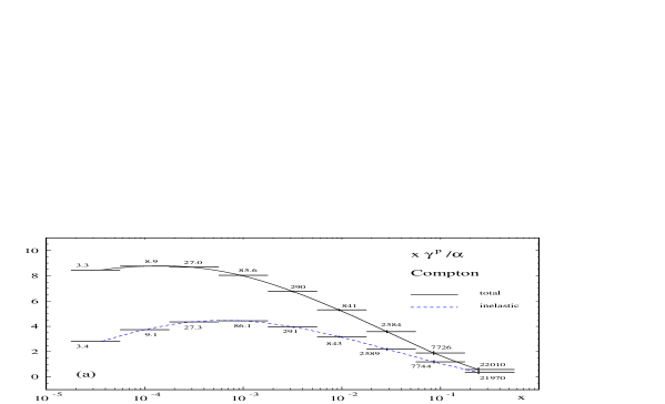
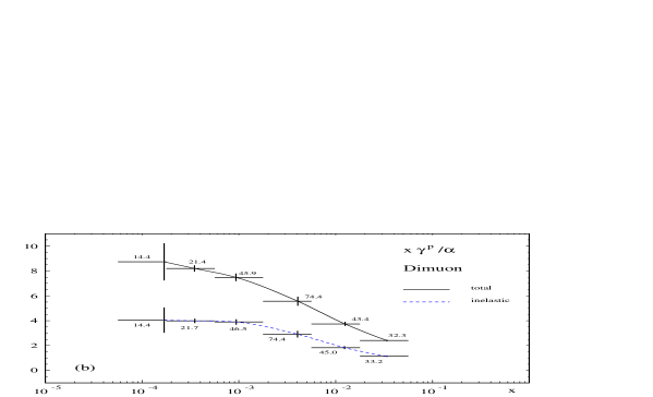
Figure 4.4: Expected statistical accuracy of the determination of $\gamma^{p}(\langle{x}\rangle,\langle{\hat{s}}\rangle)$ via the (a) QED Compton process and (b) the dimuon production process at the HERA collider. The numbers indicate the average scale $\langle{\hat{s}}\rangle$ (in GeV² units) for each $x$-bin.

Figure 4.5: Event rates for the QED Compton process at HERMES using an (un)polarized proton target. The upper (solid and dashed) curves refer to an unpolarized proton, whereas the lower ones refer to a polarized proton target. The cuts applied are as described in the text.

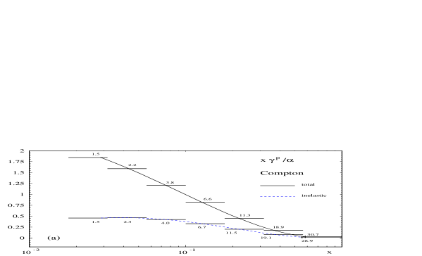
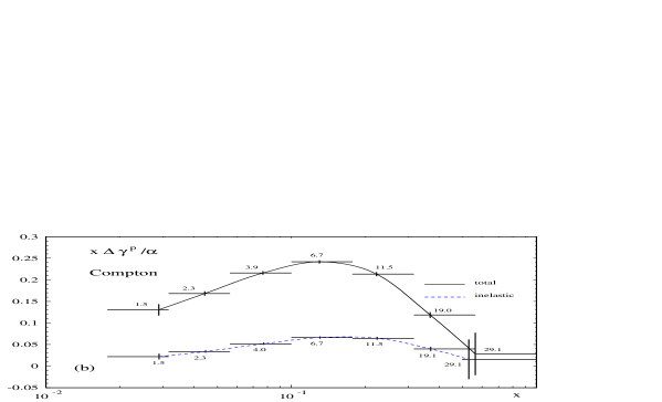
Figure 4.6: Expected statistical accuracy of the determination of (a) $\gamma^{p}(\langle{x}\rangle,\langle{\hat{s}}\rangle)$ and (b) $\Delta\gamma^{p}(\langle{x}\rangle,\langle{\hat{s}}\rangle)$ via the QED Compton process at HERMES using an (un)polarized proton target. The numbers indicate the average scale $\langle{\hat{s}}\rangle$ (in GeV² units) for each bin.

Figure 4.7: As in Figure 4.5 but for a neutron target. The negative signs at some lower-$x$ bins indicate that the polarized total cross section and/or inelastic contribution is negative.

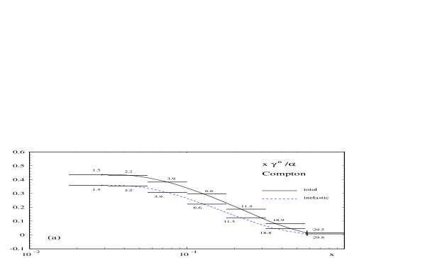
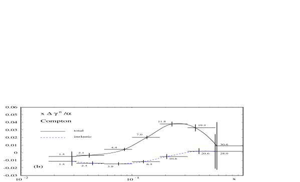
Figure 4.8: As in Figure 4.6 but for a neutron target.

Figure 4.9: As in Figure 4.5 but for dimuon production at HERMES using (un)polarized proton and neutron targets. The lower solid and dashed curves refer to a polarized nucleon target and the negative signs indicate that the polarized cross sections are negative.

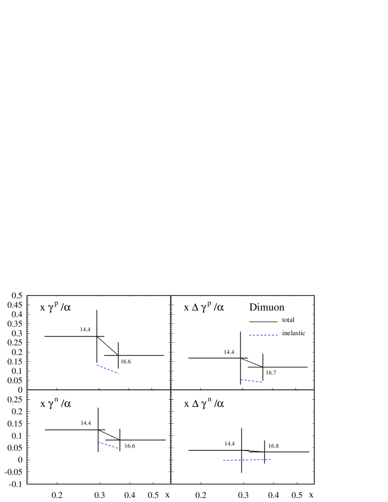
Figure 4.10: As in Figure 4.6 but for dimuon production at HERMES for (un)polarized proton and neutron targets. The statistical accuracy for the inelastic contributions is similar to those shown for the total result, except for the almost vanishing $\Delta\gamma^{n}_{\rm inel}$.

The relevant integration ranges at HERA are fixed via

$$0\leq\xi\leq 1,~{}~{}~{}~{}~{}~{}~{}~{}~{}~{}~{}~{}\frac{\hat{s}_{\rm min}}{4\xi E_{e}E_{p}}\leq x\leq 1,$$ (4.45)

with $\hat{s}$ given by $\hat{s}=4x\xi E_{e}E_{p}$ while $\eta_{i}$ are constrained by

$$\eta_{1}+\eta_{2}=\ln\frac{xE_{p}}{\xi E_{e}}~{},$$ (4.46)

which follows from (4.27) and (4.28). The relation

$$\eta_{i}-\eta_{j}=\ln\left[\frac{\xi E_{e}}{E_{i}}(1+e^{2\eta_{i}})-1\right],$$ (4.47)

as obtained from the outgoing particle energy $E_{i}=p_{T}\cosh\eta_{i}$ and its transverse momentum (4.33), further restricts the integration range of $\eta_{i,j}$ as dictated by $E_{i}\geq(E_{i})_{\rm min}$. For the QED Compton scattering process (4.41), $\xi=1$, $\eta_{1}=\eta_{e}$, $\eta_{2}=\eta_{\gamma}$ in (4.45)-(4.47). At HERMES $E_{p}\to m/2$ and $\eta_{i}\to-\eta_{i}$ in the above expressions with $\eta_{i}$ the outgoing particle rapidity with respect to the ingoing lepton direction.

In the following we shall consider $E_{\rm min}=4\ \mathrm{GeV}$. For the QED Compton scattering process we further employ $\hat{s}_{\rm min}=1\ \mathrm{GeV^{2}}$ so as to guarantee the applicability of perturbative QCD, i.e., the relevance of the utilized $\gamma^{p}(x,\hat{s})$, see (4.3) with $\mu^{2}=\hat{s}$. For the dimuon production process we shall impose $\hat{s}_{\rm min}=m^{2}[\Psi(2S)]=(3.7\ \mathrm{GeV})^{2}$ so as to evade the dimuon background induced by charmonium decays at HERMES (higher charmonium states have negligible branching ratios into dimuons); for HERA we impose in addition $\hat{s}_{\rm max}=m^{2}[\Upsilon(1S)]=(9.4\ \mathrm{GeV})^{2}$ in order to avoid the dimuon events induced by bottomium decays. Finally, at HERA we consider $\eta_{\rm min}=-3.8$, $\eta_{\rm max}=3.8$ and at HERMES $\eta_{\rm min}=2.3$, $\eta_{\rm max}=3.9$. The integrated luminosities considered are ${\cal L}_{\rm HERA}=100\ \mathrm{pb}^{-1}$ and ${\cal L}_{\rm HERMES}=1\ \mathrm{fb}^{-1}$.

In Figure 4.3 the histograms depict the expected number of dimuon and QED Compton events at HERA found by integrating (4.30) and (4.41) applying the aforementioned cuts and constraints. The important inelastic contribution due to $\gamma^{p}_{\rm inel}$, being calculated according to (4.3) using the minimal boundary condition, is shown separately by the dashed curves.

To illustrate the experimental extraction of $\gamma^{p}(x,\hat{s})$ we translate the information in Figure 4.3 into a statement on the accuracy of a possible measurement by evaluating $\gamma^{p}(\langle{x}\rangle,\langle{\hat{s}}\rangle)$ at the averages $\langle{x}\rangle$, $\langle{\hat{s}}\rangle$ determined from the event sample in Figure 4.3. Assuming that in each bin the error is only statistical, i.e. $\delta\gamma^{p}=\pm\gamma^{p}/\sqrt{N_{\rm bin}}$, the results for $x\gamma^{p}/\alpha$ are shown in Figure 4.4. It should be noticed that the statistical accuracy shown will increase if $\gamma^{p}_{\rm inel}(x,\mu_{0}^{2})\neq 0$ in contrast to our vanishing boundary condition used in all our present calculations. Our results for the QED Compton process in Figures 4.3 and 4.4 are, apart from our somewhat different cut requirements, similar to the ones presented in [27].

Apart from testing $\gamma^{p}(x,\hat{s})$ at larger values of $x$, the fixed-target HERMES experiment can measure the polarized $\Delta\gamma^{p}(x,\hat{s})$ as well. In Figure 4.5 we show the expected number of QED Compton events for an (un)polarized proton target.

The accuracy of a possible measurement of $\gamma^{p}(\langle{x}\rangle,\langle{\hat{s}}\rangle)$ and $\Delta\gamma^{p}(\langle{x}\rangle,\langle{\hat{s}}\rangle)$ is illustrated in Figure 4.6 where the averages $\langle{x}\rangle$, $\langle{\hat{s}}\rangle$ are determined from the event sample in Figure 4.5 by assuming that the error is only statistical also for the polarized photon distribution, i.e. $\delta(\Delta\gamma^{p})=\pm(\sqrt{N_{\rm bin}}/|\Delta N_{\rm bin}|)\Delta\gamma^{p}$.

The analogous expectations for an (un)polarized neutron target are shown in Figures 4.7 and 4.8. It should be pointed out that, according to Figures 4.6(b) and 4.8(b), HERMES measurements will be sufficiently accurate to delineate even the polarized $\Delta\gamma^{p,n}$ distributions in the medium- to small-$x$ region, in particular the theoretically more speculative inelastic contributions.

For completeness, in Figures 4.9 and 4.10 we also show the results for dimuon production at HERMES for (un)polarized proton and neutron targets despite the fact that the statistics will be far inferior to the Compton process.

The dimuon production can obviously proceed also via the genuine Drell- Yan subprocess $q\bar{q}\to\mu^{+}\mu^{-}$ where one of the (anti)quarks resides in the resolved component of the photon emitted by the electron. However, as already noted in [79], this contribution is negligible as compared to the one due to the Bethe- Heitler subprocess $\gamma\gamma\to\mu^{+}\mu^{-}$. The unpolarized dimuon production rates at HERA where also studied in [79, 80] utilizing, however, different prescriptions for the photon content of the nucleon.
Exact expressions for the Bethe-Heitler contribution to the longitudinally polarized $\gamma N\to\mu^{+}\mu^{-}X$ process are presented in [81] but no estimates for the expected production rates at, say, HERMES or COMPASS are given.

4.3 Summary

The analysis of the production rates of lepton-photon and muon pairs at the colliding beam experiments at HERA and the fixed-target HERMES facility, as evaluated in the leading order equivalent photon approximation, demonstrates the feasibility of determining the polarized and unpolarized equivalent photon distributions of the nucleon in the available kinematical regions. The above mentioned production rates can obviously be determined in a more accurate calculation along the lines of [34], involving the polarized and unpolarized structure functions $g_{1,2}$ and $F_{1,2}$, respectively, of the nucleon. The expected production rates are similar to those obtained in our equivalent photon approximation, as discussed in detail in the next chapters. It thus turns out that lepton-photon and muon pair production at HERA and HERMES may provide an additional and independent source of information concerning these structure functions.

Chapter 5 The Unpolarized QED Compton Scattering Process

The QED Compton scattering in high energy electron-proton collisions $ep\rightarrow e\gamma X$ is one of the most important processes for an understanding of the photon content of the proton. In addition, it can also shed some light on the proton structure functions $F_{1,2}(x_{B},Q^{2})$ [31, 34, 33] in the low-$Q^{2}$ region, where they are presently poorly known [26].

The QED Compton scattering has been recently analyzed in [31], where the above mentioned alternative descriptions were confronted with the experimental data and it was found that the description in terms of $F_{1,2}$, i.e. for $X\not=p$, is superior to the one in terms of the inelastic photon distribution $\gamma^{p}_{\mathrm{inel}}(x_{B},Q^{2})$. Henceforth we shall refer to the description in terms of $F_{1,2}$ as exact to distinguish it from the approximations involved in the EPA.

It should be noted, however, that the analysis in [31, 34] utilized the Callan-Gross relation [46] $F_{L}(x_{B},Q^{2})=F_{2}(x_{B},Q^{2})-2x_{B}F_{1}(x_{B},Q^{2})=0$. This relation is contaminated by higher order (NLO) QCD corrections as well as by higher twist contributions relevant in the low-$Q^{2}$ region which may invalidate the assumptions underlying the exact analysis. Furthermore, the analysis in [31, 34] was carried out within the framework of the helicity amplitude formalism [34]. The implementation of experimental cuts within this formalism is nontrivial and affords therefore an iterative numerical approximation procedure [34, 82] whose first step corresponds to $-k^{2}=Q^{2}=0$, where $k$ is the momentum of the virtual photon.

It is this second issue that we intend to study here. We shall replace the noncovariant helicity amplitude analysis of [34] by a standard covariant tensor analysis whose main advantage, besides compactness and transparency, is the possibility to implement the experimental cuts directly and thus avoid the necessity of employing an iterative approximation of limited accuracy. The first issue concerning the $F_{L}$ contributions affords some estimates of this poorly known structure function and we refrain from its study here.

In Section 5.1 it is specified what QED Compton scattering is and how it can be selected from the reaction $ep\rightarrow e\gamma X$. In Sections 5.2 and 5.3, we calculate its exact cross section for the elastic and inelastic channels. The numerical results are discussed in Section 5.4. The summary is given in Section 5.5 and the kinematics in Appendix C.

5.1 Radiative Corrections to Electron-Proton Collisions

The lowest order Feynman diagrams describing the process $ep\rightarrow e\gamma X$, with a real photon emission from the electron side, are shown in Figure 5.1. The corresponding amplitudes contain the denominators $k^{2}(k^{\prime}+l^{\prime})^{2}$ and $k^{2}(l-k^{\prime})^{2}$, therefore the main contributions to the cross section come from configurations where one or both denominators tend to zero. These configurations have different experimental signatures and they are described in the following [34, 31].

• The dominant contribution stems from the so-called bremsstrahlung process, which corresponds to a configuration where $k^{2}$, $(l^{\prime}+k^{\prime})^{2}$, $(l-k^{\prime})^{2}$ stay all close to zero. It involves quite large counting rates but in order to be measured, requires a specific small-angle detector, because the outgoing electron and photon have small polar angles and escape through the beam pipe.

  

  Figure 5.1: Feynman diagrams considered for $ep\rightarrow e\gamma X$, with a real final state photon $(k^{\prime 2}=0$).

• Either $(l^{\prime}+k^{\prime})^{2}\simeq 0$ or $(l-k^{\prime})^{2}\simeq 0$, but the momentum squared of the exchanged virtual photon $k^{2}$ is finite: the outgoing photon is emitted either along the final or the incoming electron line and this configuration corresponds to the so called radiative corrections to electron-proton scattering.

  In the first case, $(l^{\prime}+k^{\prime})^{2}\simeq 0$, the cross section is dominated by the contribution given by the first diagram, and this kind of events is called Final State Radiation (FSR). It is usually very difficult to distinguish this process experimentally from non-radiative deep inelastic scattering $ep\rightarrow eX$, since the outgoing electron and photon are almost collinear.

  In the second case, $(l-k^{\prime})^{2}\simeq 0$, the main contribution to the cross section is given by the second Feynman diagram in Figure 5.1 and such events are classified as Initial State Radiation (ISR). In the detector one observes only the outgoing electron, the final photon being emitted along the incident electron line.

• The virtuality of the exchanged photon is small, $k^{2}\simeq 0$, but both $(l^{\prime}+k^{\prime})^{2}$ and $(l-k^{\prime})^{2}$ are finite: the produced hadronic system goes straightforwardly along the incident proton line, the outgoing electron and photon are detected under large polar angles and almost back-to-back in azimuth, so that their total transverse momentum is close to zero. This configuration is referred to as QED Compton scattering, since it involves the scattering of a quasi-real photon on an electron. This process will thus be selected by performing a cut on the total transverse momentum of the outgoing electron and photon or on the acoplanarity (5.47) of the electron-photon system.

  As pointed out in [26], the corresponding cross section is large, despite the fact that it contains an additional factor $\alpha=1/137$ compared to the tree-level cross section for $ep\rightarrow eX$. This follows since the emission of a large transverse momentum photon can lead to a reduction of the true momentum squared transferred to the proton: $(l-l^{\prime})^{2}$ in $ep\rightarrow eX$ is shifted to $(l-l^{\prime}-k^{\prime})^{2}$ in $ep\rightarrow e\gamma X$, which can become of the order of the proton mass squared or even smaller, as will be discussed below, see (5.45). The reduction in $Q^{2}$ and the corresponding increase of the cross section in (5.40), compensates for the smallness of the additional factor $\alpha$. Hence QED Compton scattering can provide a tool to investigate the small-$Q^{2}$ behaviour of the proton structure functions. The first measurements of $F_{2}$ using QED Compton scattering have been published by the H1 collaboration at HERA [33].

5.2 Elastic QED Compton Scattering

We consider elastic QED Compton scattering:

$$e(l)+p(P)\rightarrow e(l^{\prime})+\gamma(k^{\prime})+p(P^{\prime}),$$ (5.1)

where the four-momenta of the particles are given in the brackets. We introduce the invariants

$$s=(P+l)^{2},~{}~{}~{}~{}~{}~{}~{}~{}~{}t=k^{2},$$ (5.2)

where $k=P-P^{\prime}$ is the four-momentum of the exchanged virtual photon. Moreover, we will make use of the Mandelstam variables (4.39) relative to the subprocess $e(l)\gamma(k)\to e(l^{\prime})\gamma(k^{\prime})$. The photon in the final state is real, $k^{\prime 2}=0$. We neglect the electron mass everywhere except when it is necessary to avoid divergences in the formulae and take the proton to be massive, $P^{2}=P^{\prime 2}=m^{2}$. The relevant Feynman diagrams for this process are shown in Figure 5.1, with $X$ being a proton and $P_{X}=P^{\prime}$. The squared matrix element can be written as

$$\overline{{\mid M_{\mathrm{el}}\mid}^{2}}=\frac{1}{t^{2}}H^{\alpha\beta}_{\mathrm{el}}(P,P^{\prime})T_{\alpha\beta}(l;l^{\prime},k^{\prime}),$$ (5.3)

where $T_{\alpha\beta}(l;l^{\prime},k^{\prime})$ is the leptonic tensor (B.31), given also in [75, 83] and $H^{\alpha\beta}_{\mathrm{el}}(P,P^{\prime})$ is the hadronic tensor defined in the first line of (2.18), with $N=p$, in terms of the electromagnetic current $J^{\alpha}_{\mathrm{em}}$. If we use the notation

$${\operatorname{d}}PS_{N}(p;p_{1},...,p_{N})=(2\pi)^{4}\delta\bigg{(}p-\sum_{i=1}^{N}p_{i}\bigg{)}\prod_{i=1}^{N}\frac{{\operatorname{d}}^{3}p_{i}}{(2\pi)^{3}2p_{i}^{0}}$$ (5.4)

for the Lorentz invariant $N$-particle phase-space element, the total cross section will be

$$\sigma_{\mathrm{el}}(s)=\frac{1}{2(s-m^{2})}\int{\operatorname{d}}PS_{2+1}(l+P;l^{\prime},k^{\prime},P^{\prime})\overline{{\mid M_{\mathrm{el}}\mid}^{2}}~{}.$$ (5.5)

Equation (5.5) can be rewritten following the technique of [24], which we slightly modify to implement the experimental cuts and constraints; in particular all the integrations will be performed numerically. Rearranging the ($2+1$)-particle phase space into a sequence of two $2$-particle ones, (5.5) becomes:

$$\sigma_{\mathrm{el}}(s)=\frac{1}{2(s-m^{2})}\int\frac{{\operatorname{d}}\hat{s}}{2\pi}\,{\operatorname{d}}PS_{2}(l+P;l^{\prime}+k^{\prime},P^{\prime})\frac{1}{t^{2}}H^{\alpha\beta}_{\mathrm{el}}(P,P^{\prime})X_{\alpha\beta}(l,k)~{}.$$ (5.6)

The tensor $X_{\alpha\beta}$ contains all the informations about the leptonic part of the process and is defined as

$$X_{\alpha\beta}(l,k)=\int{\operatorname{d}}PS_{2}(l+k;l^{\prime},k^{\prime})T_{\alpha\beta}(l;l^{\prime},k^{\prime})$$ (5.7)

and $T_{\alpha\beta}$ can be written as [3]

$$T_{\alpha\beta}(l;l^{\prime},k^{\prime})=\,\frac{4e^{4}}{\hat{s}\hat{u}}\,\bigg{\{}\,\frac{1}{2}\,g_{\alpha\beta}\,(\hat{s}^{2}+\hat{u}^{2}+2\hat{t}t)+2\hat{s}\,l_{\alpha}l_{\beta}+2\hat{u}\,l_{\alpha}^{\prime}l_{\beta}^{\prime}~{}~{}~{}~{}~{}~{}~{}~{}~{}~{}~{}~{}~{}~{}~{}~{}~{}~{}$$

$$~{}~{}~{}+\,(\hat{t}+t)(l_{\alpha}l_{\beta}^{\prime}+l_{\beta}l_{\alpha}^{\prime})-({\hat{s}}-t)\,(l_{\alpha}k_{\beta}^{\prime}+l_{\beta}k_{\alpha}^{\prime})~{}~{}~{}~{}~{}~{}~{}~{}$$

$$+\,(\hat{u}-t)\,(l_{\alpha}^{\prime}k_{\beta}^{\prime}+l_{\beta}^{\prime}k_{\alpha}^{\prime})\bigg{\}}.$$ (5.8)

It can be shown that

$${\operatorname{d}}PS_{2}(l+k;l^{\prime},k^{\prime})=\frac{{\operatorname{d}}\hat{t}\,{\operatorname{d}}\varphi^{*}}{16\,\pi^{2}(\hat{s}-t)}~{},$$ (5.9)

with $\varphi^{*}$ denoting the azimuthal angle of the outgoing $e-\gamma$ system in the $e-\gamma$ center-of-mass frame. For unpolarized scattering, $X_{\alpha\beta}$ is symmetric in the indices $\alpha$, $\beta$ and can be expressed in terms of two Lorentz scalars, $\tilde{X}_{1}$ and $\tilde{X}_{2}$:

$$X_{\alpha\beta}(l,k) = \frac{1}{2t}\bigg{\{}[3\tilde{X}_{1}(\hat{s},t)+\tilde{X}_{2}(\hat{s},t)]\bigg{(}\frac{2t}{\hat{s}-t}\,l-k\bigg{)}_{\alpha}\bigg{(}\frac{2t}{\hat{s}-t}\,l-k\bigg{)}_{\beta}$$ (5.10)

$$~{}~{}~{}~{}~{}+[\tilde{X}_{1}(\hat{s},t)+\tilde{X}_{2}(\hat{s},t)](tg_{\alpha\beta}-k_{\alpha}k_{\beta})\bigg{\}},$$

with

$$\tilde{X}_{1}(\hat{s},t)=\frac{4t}{(\hat{s}-t)^{2}}l^{\alpha}l^{\beta}X_{\alpha\beta}(l,k),$$ (5.11)

$$\tilde{X}_{2}(\hat{s},t)=g^{\alpha\beta}X_{\alpha\beta}(l,k).$$ (5.12)

Using the leptonic tensor (5.8) and also the relations

$$l\cdot k=\frac{1}{2}\,(\hat{s}-t),~{}~{}~{}~{}l\cdot P=\frac{1}{2}\,(s-m^{2}),~{}~{}~{}k\cdot P=\frac{1}{2}\,t,$$ (5.13)

we obtain

$$\frac{t\,l^{\alpha}l^{\beta}T_{\alpha\beta}}{4\pi^{2}(\hat{s}-t)^{3}}=\,{e^{4}}\,\frac{-t\hat{t}}{2\pi^{2}(\hat{s}-t)^{3}}\equiv X_{1}(\hat{s},t,\hat{t}),$$ (5.14)

$$\frac{g^{\alpha\beta}T_{\alpha\beta}}{16\pi^{2}(\hat{s}-t)}=\,{e^{4}}\,\frac{(t^{2}-2t\hat{s}+2\hat{s}^{2}+2\hat{s}\hat{t}+\hat{t}^{2})}{4\pi^{2}\hat{s}(\hat{s}-t)(t-\hat{s}-\hat{t})}\equiv X_{2}(\hat{s},t,\hat{t}).$$ (5.15)

The invariants $X_{i}(\hat{s},t,\hat{t})$, with $i=1,2$, are related to $\tilde{X}_{i}(\hat{s},t)$ by

$$\tilde{X}_{i}(\hat{s},t)=2\pi\int_{\hat{t}_{\mathrm{min}}}^{\hat{t}_{\mathrm{max}}}{\operatorname{d}}\hat{t}\,{X}_{i}(\hat{s},t,\hat{t}).$$ (5.16)

The integration limits of $\hat{t}$ are:

$$\hat{t}_{\mathrm{max}}=0,~{}~{}~{}~{}\hat{t}_{\mathrm{min}}=-\hat{s}+t+\frac{\hat{s}}{\hat{s}-t}\,m_{e}^{2},$$ (5.17)

where $m_{e}$ is the mass of the electron. We point out that the kinematical cuts employed by us prevent the electron propagators to become too small and thus the divergences are avoided, so we can safely neglect the electron mass in the numerial calculation. The hadronic tensor in the case of elastic scattering can be expressed in terms of the common proton form factors as in (3.7), namely

$$H^{\alpha\beta}_{\mathrm{el}}(P,P^{\prime})=e^{2}\,[H_{1}(t)(2P-k)^{\alpha}(2P-k)^{\beta}+G_{M}^{2}(t)(tg^{\alpha\beta}-k^{\alpha}k^{\beta})],$$ (5.18)

where $H_{1}(t)$, already introduced in (3.3), is given by

$$H_{1}(t)=\frac{G_{E}^{2}(t)-(t/4\,m^{2})\,G_{M}^{2}(t)}{1-{t/4\,m^{2}}}~{}.$$ (5.19)

Using

$${\operatorname{d}}PS_{2}(l+P;l^{\prime}+k^{\prime},P^{\prime})=\frac{{\operatorname{d}}t}{8\pi(s-m^{2})}~{},$$ (5.20)

finally we get [3]

$$\sigma_{\mathrm{el}}(s) = \frac{\alpha}{8\pi(s-m^{2})^{2}}\int_{\hat{s}_{\mathrm{min}}}^{(\sqrt{s}-m)^{2}}{\operatorname{d}}\hat{s}\int_{t_{\mathrm{min}}}^{t_{\mathrm{max}}}{{\operatorname{d}}t\over t}\int_{\hat{t}_{\mathrm{min}}}^{\hat{t}_{{\mathrm{max}}}}{\operatorname{d}}\hat{t}\int_{0}^{2\pi}{\operatorname{d}}\varphi^{*}\bigg{\{}\bigg{[}2\,{s-m^{2}\over\hat{s}-t}$$ (5.21)

$$\times\bigg{(}{s-m^{2}\over\hat{s}-t}-1\bigg{)}[3X_{1}(\hat{s},t,\hat{t})+X_{2}(\hat{s},t,\hat{t})]+{2m^{2}\over t}[X_{1}(\hat{s},t,\hat{t})+X_{2}(\hat{s},t,\hat{t})]$$

$$~{}~{}~{}~{}~{}~{}~{}~{}~{}~{}~{}~{}~{}~{}~{}~{}~{}~{}~{}~{}~{}~{}~{}~{}~{}+X_{1}(\hat{s},t,\hat{t})\bigg{]}H_{1}(t)+X_{2}(\hat{s},t,\hat{t})G_{M}^{2}(t)\bigg{\}},$$

where $\hat{s}_{\mathrm{min}}$ denotes the minimum of $\hat{s}$ and $t_{\mathrm{min},\,{\mathrm{max}}}$ are given by

$$t_{\mathrm{min},\,{\mathrm{max}}}=2m^{2}-{1\over 2s}\Big{[}(s+m^{2})(s-\hat{s}+m^{2})\pm(s-m^{2})\sqrt{(s-\hat{s}+m^{2})^{2}-4sm^{2}}\,\Big{]}.$$

It is to be noted that in (5.21) we have shown the integration over $\varphi^{*}$ explicitly, because of the cuts that we shall impose on the integration variables for the numerical calculation of the cross section. The cuts are discussed in Section 5.4.

The EPA consists of considering the exchanged photon as real, so it is particularly good for the elastic process in which the virtuality of the photon $|t|$ is constrained to be small ($\lesssim 1\,\mathrm{GeV}^{2}$) by the form factors. It is possible to get the approximated cross section $\sigma_{\mathrm{el}}^{\mathrm{EPA}}$ from the exact one in a straightforward way, following again [24]. If the invariant mass of the system $e-\gamma$ is large compared to the proton mass, $\hat{s}_{\mathrm{min}}\gg m^{2}$, one can neglect $|t|$ versus $\hat{s}$, $m^{2}$ versus $s$, then

$${X}_{1}(\hat{s},t,\hat{t})\approx{X}_{1}(\hat{s},0,\hat{t})=0,$$ (5.23)

and

$${X}_{2}(\hat{s},t,\hat{t})\approx{X}_{2}(\hat{s},0,\hat{t})=-{{2\hat{s}}\over{\pi}}\,{{{\operatorname{d}}\hat{\sigma}(\hat{s},\hat{t})}\over{{\operatorname{d}}\hat{t}}}~{},$$ (5.24)

where the differential cross section for the real photoproduction process $e\gamma\rightarrow e\gamma$ is given in (B.34). We get:

$$\sigma_{\mathrm{el}}(s)\approx\sigma_{\mathrm{el}}^{\mathrm{EPA}}=\int_{x_{\mathrm{min}}}^{(1-{m/\sqrt{s}})^{2}}\,{\operatorname{d}}x\,\int_{m_{e}^{2}-\hat{s}}^{0}{\operatorname{d}}\hat{t}\,\gamma^{p}_{\mathrm{el}}(x)\,{{\operatorname{d}}\hat{\sigma}(xs,\hat{t})\over{\operatorname{d}}\hat{t}}~{},$$ (5.25)

where $x={\hat{s}/s}$ and $\gamma^{p}_{\mathrm{el}}(x)$ is the elastic contribution to the equivalent photon distribution of the proton (3.2):

$$\gamma^{p}_{\mathrm{el}}(x)=-{\alpha\over 2\pi}x\int_{t_{\mathrm{min}}}^{t_{\mathrm{max}}}{{\operatorname{d}}t\over t}\bigg{\{}2\bigg{[}{1\over x}\bigg{(}{1\over x}-1\bigg{)}+{m^{2}\over t}\bigg{]}H_{1}(t)+G_{M}^{2}(t)\bigg{\}},$$ (5.26)

with

$${t_{\mathrm{min}}\approx-\infty}~{}~{}~{}~{}~{}~{}~{}~{}~{}~{}~{}~{}t_{\mathrm{max}}\approx-{{m^{2}x^{2}}\over{1-x}}~{}.$$ (5.27)

To clarify the physical meaning of $x$, let us introduce the variable $x_{\gamma}$:

$$x_{\gamma}={{l\cdot k}\over{P\cdot l}}~{}.$$ (5.28)

It is possible to show that $x_{\gamma}$ represents the fraction of the longitudinal momentum of the proton carried by the virtual photon, so that one can write

$$k=x_{\gamma}P+\hat{k},$$ (5.29)

with $\hat{k}\cdot l=0$. Using (5.2) one gets

$$x_{\gamma}={{\hat{s}-t}\over{s-m^{2}}}~{},$$ (5.30)

which reduces to $x$ in the EPA limit, see also (3.10) and (3.11). One can also define the leptonic variable $x_{l}$:

$$x_{l}={{Q^{2}_{l}}\over{2P\cdot(l-l^{\prime})}}~{},$$ (5.31)

where $Q^{2}_{l}=-\hat{t}$. When $t\simeq 0$, it turns out that also $x_{l}\simeq x$.

5.3 Inelastic QED Compton Scattering

To calculate the inelastic QED Compton scattering cross section, we extend the approach discussed in the previous section. In this case, an electron and a photon are produced in the final state with a general hadronic system $X$. In other words, we consider the process

$$e(l)+p(P)\rightarrow e(l^{\prime})+\gamma(k^{\prime})+X(P_{X}),$$ (5.32)

where $P_{X}=\sum_{X_{i}}P_{X_{i}}$ is the sum over all momenta of the produced hadrons. Let the invariant mass of the produced hadronic state $X$ to be $W$; (5.2) still holds with $Q^{2}=-t$. The cross section for inelastic scattering will be

$$\sigma_{\mathrm{inel}}(s)={1\over{2(s-m^{2})}}\int{\operatorname{d}}PS_{2+N}(l+P;l^{\prime},k^{\prime},P_{X_{1}},...,P_{X_{N}})\overline{{\mid M_{\mathrm{inel}}\mid}^{2}},$$ (5.33)

where

$$\overline{{\mid M_{\mathrm{inel}}\mid}^{2}}={1\over Q^{4}}H^{\alpha\beta}_{\mathrm{inel}}(P,P_{X})T_{\alpha\beta}(l,k;l^{\prime},k^{\prime})$$ (5.34)

is the squared matrix element and the tensor $H^{\alpha\beta}_{\mathrm{inel}}(P,P_{X})$ has already been introduced in (2.42). If we rearrange the ($2+N$)-particle space phase into a sequence of a $2$-particle and a $N$-particle one, we get

$$\sigma_{\mathrm{inel}}(s)={1\over 2(s-m^{2})}\int{{\operatorname{d}}W^{2}\over 2\pi}\int{{\operatorname{d}}\hat{s}\over 2\pi}\int{\operatorname{d}}PS_{2}(l+P;l^{\prime}+k^{\prime},P_{X}){1\over Q^{4}}W^{\alpha\beta}(P,k)X_{\alpha\beta}(l,k),$$

where $X_{\alpha\beta}$ is given by (5.10) and $W^{\alpha\beta}$ is the hadronic tensor for inelastic scattering defined in (2.41), that is, using the notation (5.4),

$$W^{\alpha\beta}=\int{\operatorname{d}}PS_{N}(P-k;P_{X_{1}},....,P_{X_{N}})\,H^{\alpha\beta}_{\mathrm{inel}}~{}.$$ (5.36)

The hadronic tensor is parametrized in terms of $F_{1}$ and $F_{2}$, the usual structure functions of the proton, as in (3.8), i.e.

$$W^{\alpha\beta} = {4\pi e^{2}\over Q^{2}}\bigg{[}-(Q^{2}g^{\alpha\beta}+k^{\alpha}k^{\beta})F_{1}(x_{B},Q^{2})$$ (5.37)

$$~{}~{}~{}~{}~{}~{}~{}~{}~{}~{}~{}~{}~{}~{}~{}~{}~{}~{}~{}~{}~{}~{}~{}~{}~{}~{}+(2x_{B}P^{\alpha}-k^{\alpha})(2x_{B}P^{\beta}-k^{\beta}){F_{2}(x_{B},Q^{2})\over 2x_{B}}\bigg{]},$$

where $x_{B}$ is the Bjorken variable (2.37),

$$x_{B}={Q^{2}\over 2P\cdot(-k)}={Q^{2}\over Q^{2}+W^{2}-m^{2}}~{}.$$ (5.38)

Using

$${\operatorname{d}}PS_{2}(l+P;l^{\prime}+k^{\prime},P_{X})={{\operatorname{d}}Q^{2}\over 8\pi(s-m^{2})}$$ (5.39)

as before, we get [3]

$$\sigma_{\mathrm{inel}}(s) = {\alpha\over 4\pi(s-m^{2})^{2}}\int_{W^{2}_{{\mathrm{min}}}}^{W^{2}_{\mathrm{max}}}{\operatorname{d}}W^{2}\int_{\hat{s}_{\mathrm{min}}}^{(\sqrt{s}-W)^{2}}{\operatorname{d}}\hat{s}\int_{Q^{2}_{\mathrm{min}}}^{Q^{2}_{\mathrm{max}}}{dQ^{2}\over Q^{4}}\int_{\hat{t}_{\mathrm{min}}}^{\hat{t}_{\rm max}}{\operatorname{d}}\hat{t}\int_{0}^{2\pi}{\operatorname{d}}\varphi^{*}$$ (5.40)

$$~{}~{}\times\bigg{\{}\bigg{[}\bigg{(}2\,{{s-m^{2}}\over{\hat{s}+Q^{2}}}\bigg{(}1-{{s-m^{2}}\over{\hat{s}+Q^{2}}}\bigg{)}+(W^{2}-m^{2})\bigg{(}{2\,(s-m^{2})\over{Q^{2}(\hat{s}+Q^{2})}}-{1\over Q^{2}}$$

$$~{}~{}~{}~{}~{}+{m^{2}-W^{2}\over 2\,Q^{4}}\bigg{)}\bigg{)}[3X_{1}(\hat{s},Q^{2},\hat{t})+X_{2}(\hat{s},Q^{2},\hat{t})]+\bigg{(}{1\over Q^{2}}(W^{2}-m^{2})$$

$$~{}~{}~{}~{}~{}~{}~{}~{}+{(W^{2}-m^{2})^{2}\over 2\,Q^{4}}+{2m^{2}\over Q^{2}}\bigg{)}[X_{1}(\hat{s},Q^{2},\hat{t})+X_{2}(\hat{s},Q^{2},\hat{t})]-X_{1}(\hat{s},Q^{2},\hat{t})\bigg{]}$$

$$~{}~{}~{}~{}~{}~{}~{}~{}~{}~{}~{}\times F_{2}(x_{B},Q^{2}){x_{B}\over 2}-X_{2}(\hat{s},Q^{2},\hat{t})F_{1}(x_{B},Q^{2})\bigg{\}}.$$

Here $X_{i}(\hat{s},Q^{2},\hat{t})$, with $\,i=1,2$, are given by (5.14)-(5.15) with $t$ replaced by $-Q^{2}$. The limits of the integration over $Q^{2}$ are:

$$Q^{2}_{{{\mathrm{min}},{\mathrm{max}}}} = -m^{2}-W^{2}+{1\over 2s}\Big{[}(s+m^{2})(s-\hat{s}+W^{2})$$ (5.41)

$$~{}~{}~{}~{}~{}~{}~{}~{}~{}~{}~{}~{}~{}~{}~{}~{}~{}~{}~{}~{}~{}~{}~{}~{}\mp(s-m^{2}){\sqrt{(s-\hat{s}+W^{2})^{2}-4sW^{2}}}\Big{]},$$

while the extrema of $\hat{t}$ are the same as (5.17). The limits $W^{2}_{\mathrm{min},\mathrm{max}}$ are given by:

$$W^{2}_{\mathrm{min}}=(m+m_{\pi})^{2},~{}~{}~{}~{}~{}~{}~{}~{}W^{2}_{\mathrm{max}}=(\sqrt{s}-\sqrt{\hat{s}_{\mathrm{min}}}\,)^{2},$$ (5.42)

where $m_{\pi}$ is the mass of the pion.

In the EPA, we neglect $m^{2}$ compared to $s$ and $Q^{2}$ compared to $\hat{s}$ as before. Using (5.23) and (5.24), we can write

$$\sigma_{\mathrm{inel}}(s)\approx\sigma_{\mathrm{inel}}^{\mathrm{EPA}}=\int_{x_{\mathrm{min}}}^{(1-m/\sqrt{s})^{2}}{\operatorname{d}}x\,\int_{m_{e}^{2}-\hat{s}}^{0}{\operatorname{d}}\hat{t}~{}\gamma^{p}_{\mathrm{inel}}(x,xs)\,{{{\operatorname{d}}\hat{\sigma}(xs,\hat{t})}\over{{\operatorname{d}}\hat{t}}}~{},$$ (5.43)

where again $x={\hat{s}/s}$ and $\gamma^{p}_{\mathrm{inel}}(x,xs)$ is the inelastic contribution to the equivalent photon distribution of the proton [84]:

$$\gamma^{p}_{\mathrm{inel}}(x,xs) = {\alpha\over 2\pi}\int_{x}^{1}\,{\operatorname{d}}y\int_{Q^{2}_{\mathrm{min}}}^{Q^{2}_{\mathrm{max}}}{{\operatorname{d}}Q^{2}\over Q^{2}}\,{y\over x}\bigg{[}F_{2}\bigg{(}{x\over y},Q^{2}\bigg{)}\bigg{(}{{1+(1-y)^{2}}\over y^{2}}-{2m^{2}x^{2}\over y^{2}Q^{2}}\bigg{)}$$ (5.44)

$$~{}~{}~{}~{}~{}~{}~{}~{}~{}~{}~{}~{}~{}~{}-F_{L}\bigg{(}{x\over y},Q^{2}\bigg{)}\bigg{]},$$

The limits of the $Q^{2}$ integration can be approximated as

$$Q^{2}_{\mathrm{min}}={x^{2}m^{2}\over 1-x}~{},$$ (5.45)

and we choose the scale $Q^{2}_{\rm{max}}$ to be $\hat{s}$. Our expression of $\gamma^{p}_{\mathrm{inel}}(x,xs)$ differs from [26] by a (negligible) term proportional to $m^{2}$. Following [31, 34] we shall use the LO Callan-Gross relation

$$F_{L}(x_{B},Q^{2})~{}=~{}F_{2}(x_{B},Q^{2})-2x_{B}F_{1}(x_{B},Q^{2})~{}=~{}0$$ (5.46)

in our numerical calculations.

5.4 Numerical Results

In this section, we present an estimate of the cross section, calculated both exactly and using the equivalent photon approximation of the proton. We have used the same kinematical cuts as used in [31] for the HERA collider, which are slightly different from the ones in [34]. They are imposed on the following laboratory frame variables: energy of the final electron $E_{e}^{\prime}$, energy of the final photon $E_{\gamma}^{\prime}$, polar angles of the outgoing electron and photon, $\theta_{e}$ and $\theta_{\gamma}$ respectively, and acoplanarity angle $\phi$, which is defined as

$$\phi=|\,\pi-|\phi_{\gamma}-\phi_{e}|\,|,$$ (5.47)

where $\phi_{\gamma}$ and $\phi_{e}$ are the azimuthal angles of the outgoing photon and electron respectively ($0\leq\phi_{\gamma},\,\phi_{e}\leq 2\,\pi$). The cuts are given by:

$$E_{e}^{\prime},E_{\gamma}^{\prime}>4\,{\mathrm{GeV}},~{}~{}~{}~{}~{}~{}~{}~{}E_{e}^{\prime}+E_{\gamma}^{\prime}>20\,{\mathrm{GeV}},$$ (5.48)

$$0.06<\theta_{e},\theta_{\gamma}<\pi-0.06,$$ (5.49)

$$0<\phi<{\pi\over 4}~{}.$$ (5.50)

The energies of the incoming particles are: $E_{e}=27.5\,\,\mathrm{GeV}$ (electron) and $E_{p}=820\,\,\mathrm{GeV}$ (proton). In our conventions, we fix the laboratory frame such that $\phi_{e}=0$, so the acoplanarity will be $\phi=|\,\pi-\phi_{\gamma}\,|$. These cuts reflect experimental acceptance constraints as well as the reduction of the background events due to emitted photons with $(l^{\prime}+k^{\prime})^{2}\approx 0$ and/or $(l-k^{\prime})^{2}\approx 0$, which are unrelated to the QED Compton scattering process (for which $-k^{2}=Q^{2}\approx 0$ but with both $(l^{\prime}+k^{\prime})^{2}$ and $(l-k^{\prime})^{2}$ finite), i.e. photons emitted parallel to the ingoing (outgoing) electron [26, 34], as discussed in Section 5.1.

In contrast to [34], we find that the cuts (5.48)-(5.50) are not sufficient to suppress the background due to photon emission at the hadron vertex, discussed in the next chapter. Such a background has been subtracted from the measurements in [31] and from the numerical estimates in [31, 32], which will be shown for comparison with our results in Figure 5.2 and in the Tables 5.1 and 5.2.

We numerically integrate the elastic and inelastic cross sections given by (5.21) and (5.40). To implement the cuts in (5.48)-(5.50), we express $E_{e}^{\prime}$, $E_{\gamma}^{\prime}$, $\cos{\theta_{e}}$, $\cos{\theta_{\gamma}}$ and $\cos{\phi}$ in terms of our integration variables $\hat{s}$, $t$, $\hat{t}$, $\varphi^{*}$ (and $W^{2}$ in the inelastic channel), as explained in Appendix C. More explicitly, we use (C.27)-(C.31), (C.12), (C.13), together with (C.16)-(C.18) for the elastic channel and (C.36)-(C.38) for the inelastic one. The cuts imposed on the laboratory frame variables restrict the range of our integrations numerically. In this way, we are able to remove the contributions from outside the considered kinematical region.

In the calculation of the elastic cross section, the electric and magnetic form factors are empirically parametrized as dipoles

$$G_{E}(t)=\frac{1}{[1-t/(0.71\,\mathrm{GeV}^{2})]^{2}}~{},~{}~{}~{}~{}G_{M}(t)=2.79~{}G_{E}(t).$$ (5.51)

Following [31], in the evaluation of (5.40) we have used the ALLM97 parametrization of the proton structure function $F_{2}(x_{B},Q^{2})$ [70], which provides a purely phenomenological, Regge model inspired, description of $F_{2}(x_{B},Q^{2})$, including its vanishing in the $Q^{2}=0$ limit as well as its scaling behaviour at large $Q^{2}$. The ALLM97 parametrization is supposed to hold over the entire range of $x_{B}$ and $Q^{2}$ studied so far, namely $3\times 10^{-6}<x_{B}<0.85$ and $0\leq Q^{2}<5000$ $\mathrm{GeV}^{2}$, above the quasi-elastic region ($W^{2}>3$ $\mathrm{GeV}^{2}$) dominated by resonances. We do not consider the resonance contribution separately but, using the so-called local duality [85], we extend the ALLM97 parametrization from the continuous ($W^{2}>3$ $\mathrm{GeV}^{2}$) down to the resonance domain ($(m_{\pi}+m)^{2}<W^{2}<3$ $\mathrm{GeV}^{2}$): in this way it is possible to agree with the experimental data averaged over each resonance, as pointed out in [31].

The elastic contribution to the EPA was calculated using (5.25) subject to the additional kinematical restrictions given by (5.48)-(5.49). For the inelastic channel we have used (5.43) together with (5.44), the cuts being the same as in the elastic case. We have taken $F_{L}=0$ and used the ALLM97 parametrization of $F_{2}$, in order to compare consistently with the exact cross section. We point out that in (3.2), as well as in [27, 1, 2], $F_{2}(x_{B},Q^{2})$ in $\gamma^{p}_{\mathrm{inel}}(x,xs)$ was expressed in terms of parton distributions for which the LO GRV98 parametrization [68] was used, together with $Q^{2}_{\mathrm{min}}=0.26~{}{\mathrm{GeV}}^{2}$ so as to guarantee the applicability of perturbative QCD [25]. The new $\gamma^{p}_{\mathrm{inel}}(x,xs)$ gives slightly higher results than the ones obtained with the photon distribution in (3.2).

Figure 5.2: Cross section for Compton process at HERA-H1. The cuts applied are given in (5.48)-(5.50).

Figure 5.3: Cross section for Compton process at HERA-H1. The bins are in $x_{\gamma}$. The cuts applied are given in (5.48)- (5.50).

Figure 5.4: Double differential cross section for QED Compton scattering at HERA-H1. The data are taken from [31]. The kinematical bins correspond to Table 5.1. The continuous line corresponds to our exact calculation, the dotted line to the calculation in [31] and the dashed line to the EPA.

The Compton process turns out to be dominated by the elastic channel, in fact after Monte Carlo integration, we find that $\sigma_{\mathrm{el}}=1.7346$ nb, while $\sigma_{\mathrm{inel}}=1.1191$ nb. The approximated calculation gives the results: $\sigma_{\mathrm{el}}^{\mathrm{EPA}}=1.7296$ nb and $\sigma_{\mathrm{inel}}^{\mathrm{EPA}}=1.5183$ nb. This means that in the kinematical region under consideration, the total (elastic + inelastic) cross section calculated using the EPA agrees with the exact one within 14% and that the approximation turns out to be particularly good in describing the elastic process, for which the agreement is within 0.3%. This is not surprising since in the EPA one assumes $Q^{2}=0$, which is not true especially in the inelastic channel and the inelastic cross section receives substantial contribution from the non-zero $Q^{2}$ region. In terms of the kinematical cuts, the EPA corresponds to the situation when the outgoing electron and the final photon are observed under large polar angles and almost opposite to each other in azimuth, so that the acoplanarity is approximately zero. For elastic scattering there is a sharp peak of the exact cross section for $\phi=0$, contributions from non-zero $\phi$ are very small in this case. But the inelastic cross section receives contribution even from non-zero $\phi$, so that in this case the discrepancy from the approximated result is higher. The discrepancy of the total cross section with the approximate one is thus entirely due to the inelastic part.

In Figure 5.2 we have compared the total cross sections (exact and EPA) in different $x_{l}$ bins, in the region $1.78\times 10^{-5}<x_{l}<1.78\times 10^{-1}$. Figure 5.3 shows that the agreement improves slightly for bins in the variable $x_{\gamma}$. Since $x_{\gamma}\simeq x_{l}$ for $Q^{2}\simeq 0$, the elastic process is not sensitive to this change of variables. We point out again that in the EPA limit ($Q^{2}=0$) $x_{l}=x_{\gamma}=x$.

In Figure 5.4 we show the exact and the EPA cross section in $x_{l}$ and $Q_{l}^{2}$ bins together with the experimental results and the estimates of the Compton event generator, already presented in [31]. Except for two bins, our exact result agrees with the experiment within the error bars. The slight difference of our exact result and the one of [31] may be due to the fact that in [31] the cross section is calculated using a Monte Carlo generator in a step by step iteration [34, 82] which starts by assuming $Q^{2}=0$, while we did not use any approximation. Our exact result is closer to the EPA in most of the kinematical bins as compared to [31]. The total cross section in the EPA lies above the exact one in most of the bins.

For completeness, we have shown the numerical values of the exact and EPA double differential cross sections, both for the elastic (Table 5.1) and inelastic (Table 5.2) contributions. The kinematical bins are the same as in [31]. The exact results when the bins are in $x_{\gamma}$ instead of $x_{l}$ are also shown.

$x$ bin	$Q^{2}_{l}$ bin	$\sigma_{\mathrm{el}}$	$\sigma_{\mathrm{el}}^{\mathrm{Len}}$	$\sigma_{\mathrm{el}}^{*}$	$\sigma_{\mathrm{el}}^{\mathrm{EPA}}$
$1.78\times 10^{-5}-5.62\times 10^{-5}$	$1.5-2.5$	$2.428\times 10^{2}$	$2.342\times 10^{2}$	$2.446\times 10^{2}$	$2.461\times 10^{2}$
$1.78\times 10^{-5}-5.62\times 10^{-5}$	$2.5-3.5$	$5.099\times 10^{1}$	$4.71\times 10^{1}$	$5.201\times 10^{1}$	$5.051\times 10^{1}$
$5.62\times 10^{-5}-1.78\times 10^{-4}$	$1.5-5.0$	$5.279\times 10^{2}$	$5.319\times 10^{2}$	$5.259\times 10^{2}$	$5.247\times 10^{2}$
$5.62\times 10^{-5}-1.78\times 10^{-4}$	$5.0-8.5$	$2.396\times 10^{2}$	$2.327\times 10^{2}$	$2.404\times 10^{2}$	$2.395\times 10^{2}$
$5.62\times 10^{-5}-1.78\times 10^{-4}$	$8.5-12.0$	$8.496\times 10^{1}$	$8.32\times 10^{1}$	$8.559\times 10^{1}$	$8.571\times 10^{1}$
$1.78\times 10^{-4}-5.62\times 10^{-4}$	$3.0-14.67$	$2.080\times 10^{2}$	$2.036\times 10^{2}$	$2.056\times 10^{2}$	$2.061\times 10^{2}$
$1.78\times 10^{-4}-5.62\times 10^{-4}$	$14.67-26.33$	$1.373\times 10^{2}$	$1.388\times 10^{2}$	$1.373\times 10^{2}$	$1.372\times 10^{2}$
$1.78\times 10^{-4}-5.62\times 10^{-4}$	$26.33-38.0$	$3.712\times 10^{1}$	$3.86\times 10^{1}$	$3.720\times 10^{1}$	$3.695\times 10^{1}$
$5.62\times 10^{-4}-1.78\times 10^{-3}$	$10.0-48.33$	$5.947\times 10^{1}$	$5.71\times 10^{1}$	$5.918\times 10^{1}$	$5.921\times 10^{1}$
$5.62\times 10^{-4}-1.78\times 10^{-3}$	$48.33-86.67$	$3.714\times 10^{1}$	$3.85\times 10^{1}$	$3.715\times 10^{1}$	$3.704\times 10^{1}$
$5.62\times 10^{-4}-1.78\times 10^{-3}$	$86.67-125.0$	$1.056\times 10^{1}$	$1.028\times 10^{1}$	$1.057\times 10^{1}$	$1.054\times 10^{1}$
$1.78\times 10^{-3}-5.62\times 10^{-3}$	$22-168$	$1.913\times 10^{1}$	$1.877\times 10^{1}$	$1.909\times 10^{1}$	$1.909\times 10^{1}$
$1.78\times 10^{-3}-5.62\times 10^{-3}$	$168-314$	$1.239\times 10^{1}$	$1.229\times 10^{1}$	$1.239\times 10^{1}$	$1.238\times 10^{1}$
$1.78\times 10^{-3}-5.62\times 10^{-3}$	$314-460$	$5.917$	$6.02$	$5.915$	$5.914$
$5.62\times 10^{-3}-1.78\times 10^{-2}$	$0-500$	$4.811$	$5.76$	$4.890$	$4.890$
$5.62\times 10^{-3}-1.78\times 10^{-2}$	$500-1000$	$9.271$	$9.22$	$9.264$	$9.271$
$5.62\times 10^{-3}-1.78\times 10^{-2}$	$1000-1500$	$2.572$	$2.65$	$2.571$	$2.573$
$1.78\times 10^{-2}-5.62\times 10^{-2}$	$0-1500$	$8.238\times 10^{-1}$	$6.8\times 10^{-1}$	$9.085\times 10^{-1}$	$9.086\times 10^{-1}$
$1.78\times 10^{-2}-5.62\times 10^{-2}$	$1500-3000$	$2.431$	$2.69$	$2.430$	$2.434$
$1.78\times 10^{-2}-5.62\times 10^{-2}$	$3000-4500$	$6.336\times 10^{-1}$	$7.7\times 10^{-1}$	$6.328\times 10^{-1}$	$6.345\times 10^{-1}$
$5.62\times 10^{-2}-1.78\times 10^{-1}$	$10-6005$	$3.120\times 10^{-1}$	$4.27\times 10^{-1}$	$3.120\times 10^{-1}$	$3.117\times 10^{-1}$
$5.62\times 10^{-2}-1.78\times 10^{-1}$	$6005-12000$	$2.437\times 10^{-1}$	$2.13\times 10^{-1}$	$2.438\times 10^{-1}$	$2.436\times 10^{-1}$
$5.62\times 10^{-2}-1.78\times 10^{-1}$	$12000-17995$	$0.000$	$0.000$	$0.000$	$2.461\times 10^{-2}$

Table 5.1: Double differential (elastic) QED Compton scattering cross section. $\sigma_{\mathrm{el}}$ is the exact result in (5.21), $\sigma_{\mathrm{el}}^{\mathrm{Len}}$ corresponds to the results in [31]. The $x$-bins refer to $x_{l}$ in (5.31) except for $\sigma_{\mathrm{el}}^{*}$ where they refer to $x_{\gamma}$ in (5.30). $\sigma_{\mathrm{el}}^{\mathrm{EPA}}$ is given in (5.25) where $x\equiv x_{\gamma}$. $Q^{2}_{l}$ is expressed in GeV² and the cross sections are in pb.

$x$ bin	$Q^{2}_{l}$ bin	$\sigma_{\mathrm{inel}}$	$\sigma_{\mathrm{inel}}^{\mathrm{Len}}$	$\sigma_{\mathrm{inel}}^{*}$	$\sigma_{\mathrm{inel}}^{\mathrm{EPA}}$
$1.78\times 10^{-5}-5.62\times 10^{-5}$	$1.5-2.5$	$7.802\times 10^{1}$	$6.170\times 10^{1}$	$7.367\times 10^{1}$	$1.483\times 10^{2}$
$1.78\times 10^{-5}-5.62\times 10^{-5}$	$2.5-3.5$	$2.799\times 10^{1}$	$2.050\times 10^{1}$	$4.029\times 10^{1}$	$3.255\times 10^{1}$
$5.62\times 10^{-5}-1.78\times 10^{-4}$	$1.5-5.0$	$2.299\times 10^{2}$	$2.296\times 10^{2}$	$2.298\times 10^{2}$	$3.967\times 10^{2}$
$5.62\times 10^{-5}-1.78\times 10^{-4}$	$5.0-8.5$	$1.108\times 10^{2}$	$1.062\times 10^{2}$	$1.450\times 10^{2}$	$2.016\times 10^{2}$
$5.62\times 10^{-5}-1.78\times 10^{-4}$	$8.5-12.0$	$3.340\times 10^{1}$	$2.890\times 10^{1}$	$6.048\times 10^{1}$	$7.751\times 10^{1}$
$1.78\times 10^{-4}-5.62\times 10^{-4}$	$3.0-14.67$	$2.029\times 10^{2}$	$2.287\times 10^{2}$	$1.228\times 10^{2}$	$2.104\times 10^{2}$
$1.78\times 10^{-4}-5.62\times 10^{-4}$	$14.67-26.33$	$9.644\times 10^{1}$	$9.230\times 10^{1}$	$1.164\times 10^{2}$	$1.476\times 10^{2}$
$1.78\times 10^{-4}-5.62\times 10^{-4}$	$26.33-38.0$	$2.742\times 10^{1}$	$2.570\times 10^{1}$	$4.431\times 10^{1}$	$4.298\times 10^{1}$
$5.62\times 10^{-4}-1.78\times 10^{-3}$	$10.0-48.33$	$1.011\times 10^{2}$	$1.064\times 10^{2}$	$5.077\times 10^{1}$	$7.555\times 10^{1}$
$5.62\times 10^{-4}-1.78\times 10^{-3}$	$48.33-86.67$	$4.485\times 10^{1}$	$4.590\times 10^{1}$	$5.304\times 10^{1}$	$4.897\times 10^{1}$
$5.62\times 10^{-4}-1.78\times 10^{-3}$	$86.67-125.0$	$1.228\times 10^{1}$	$1.132\times 10^{1}$	$1.887\times 10^{1}$	$1.462\times 10^{1}$
$1.78\times 10^{-3}-5.62\times 10^{-3}$	$22-168$	$4.320\times 10^{1}$	$4.917\times 10^{1}$	$2.225\times 10^{1}$	$2.791\times 10^{1}$
$1.78\times 10^{-3}-5.62\times 10^{-3}$	$168-314$	$1.831\times 10^{1}$	$1.735\times 10^{1}$	$2.117\times 10^{1}$	$1.849\times 10^{1}$
$1.78\times 10^{-3}-5.62\times 10^{-3}$	$314-460$	$6.314$	$5.760$	$8.303$	$9.046$
$5.62\times 10^{-3}-1.78\times 10^{-2}$	$0-500$	$1.277\times 10^{1}$	$1.432\times 10^{1}$	$6.438$	$7.627$
$5.62\times 10^{-3}-1.78\times 10^{-2}$	$500-1000$	$1.086\times 10^{1}$	$9.890$	$1.152\times 10^{1}$	$1.450\times 10^{1}$
$5.62\times 10^{-3}-1.78\times 10^{-2}$	$1000-1500$	$2.734$	$2.600$	$3.201$	$4.067$
$1.78\times 10^{-2}-5.62\times 10^{-2}$	$0-1500$	$2.787$	$2.500$	$1.321$	$1.439$
$1.78\times 10^{-2}-5.62\times 10^{-2}$	$1500-3000$	$3.118$	$2.150$	$3.149$	$3.855$
$1.78\times 10^{-2}-5.62\times 10^{-2}$	$3000-4500$	$7.718\times 10^{-1}$	$6.600\times 10^{-1}$	$8.421\times 10^{-1}$	$1.004$
$5.62\times 10^{-2}-1.78\times 10^{-1}$	$10-6005$	$7.203\times 10^{-1}$	$1.460\times 10^{-1}$	$4.677\times 10^{-1}$	$4.924\times 10^{-1}$
$5.62\times 10^{-2}-1.78\times 10^{-1}$	$6005-12000$	$3.739\times 10^{-1}$	$2.110\times 10^{-1}$	$3.830\times 10^{-1}$	$3.845\times 10^{-1}$
$5.62\times 10^{-2}-1.78\times 10^{-1}$	$12000-17995$	$3.738\times 10^{-2}$	$4.300\times 10^{-2}$	$4.182\times 10^{-2}$	$3.849\times 10^{-2}$

Table 5.2: Double differential (inelastic) QED Compton scattering cross section. $\sigma_{\mathrm{inel}}$ is the exact result in (5.40), $\sigma_{\mathrm{inel}}^{\mathrm{Len}}$ corresponds to the results in [31]. The $x$-bins are as in Table 5.1, i.e. refer to $x_{l}$ in (5.31) except for $\sigma_{\mathrm{inel}}^{*}$ where they refer to $x_{\gamma}$ in (5.30). $\sigma_{\mathrm{inel}}^{\mathrm{EPA}}$ is given in (5.43) where $x\equiv x_{\gamma}$. $Q^{2}_{l}$ is expressed in GeV² and the cross sections are in pb.

The EPA elastic cross section agrees within $1\%$ with the exact one for all the $x_{l}$ bins. The agreement becomes slightly better if we consider $x_{\gamma}$ bins. For the inelastic channel, the discrepancies from the EPA results are considerably higher. Our ’exact’ results lie closer to the EPA compared to [31] in almost all the bins. The result in $x_{\gamma}$ bins shows better agreement with the EPA compared to the $x_{l}$ bins, especially for higher $x_{\gamma}$. The discrepancy with the EPA is about $20-30\%$ in most of the bins, higher in some cases.

5.5 Summary

In this chapter, we have estimated both the elastic and the inelastic QED Compton scattering cross sections for unpolarized incoming electron and proton. Our approach for the calculation of the total cross section is manifestly covariant and we have used the same cuts as in [31]. The numerical estimates of the exact cross section for different kinematical bins are presented and compared with the EPA and the experimental results. The exact cross section in the elastic channel agrees within $1\%$ with the approximate one. The discrepancy is thus due to the inelastic channel and, in the next chapter, new cuts will be suggested in order to reduce it. A comparison with the Monte Carlo results of [31] is also shown. For both elastic and inelastic cross sections, our exact results are closer to the EPA as compared to [31]. The agreement is even better if the bins are in $x_{\gamma}$ instead of $x_{l}$.

Chapter 6 Suppression of the Background to QED Compton scattering

In this chapter we perform a detailed study of the QED Compton scattering process (QEDCS) in $ep\rightarrow e\gamma p$ and $ep\rightarrow e\gamma X$, depicted in Figure 6.1, together with the major background coming from the virtual Compton scattering (VCS), where the photon is emitted from the hadronic vertex, shown in Figure 6.2. The two processes can be distinguished experimentally because they differ in the kinematic distributions of the outgoing electron and photon. We suggest new kinematical cuts to suppress the VCS background, which turns out to be important in the phase space domain of the HERA experiment. We also study the impact of these constraints on the QEDCS cross section. We show that in the phase space region suggested and accessible at HERA, the photon content of the proton provides a reasonably good description of the QEDCS cross section, also in the inelastic channel.

The VCS cross section in the inelastic channel is estimated utilizing effective parton distributions of the proton. In the elastic channel, to make a relative estimate of the VCS, we take the proton to be pointlike and replace the vertex by an effective vertex [4].

In Sections 6.1 and 6.2 we present the cross section in the elastic and inelastic channels respectively. Numerical results are given in Section 6.3. The summary is presented in Section 6.4. The matrix elements are explicitly shown in Appendix D.

Figure 6.1: Feynman diagrams for the QED Compton process (QEDCS). $X\equiv p$ (and $P_{X}\equiv P^{\prime}$) corresponds to elastic scattering.

Figure 6.2: As in Figure 6.1 but for the virtual Compton scattering (VCS) background process.

6.1 Elastic Channel

The elastic channel of the process under study,

$$e(l)+p(P)\rightarrow e(l^{\prime})+p(P^{\prime})+\gamma(k^{\prime}),$$ (6.1)

is described by the Feynman diagrams in Figures 6.1 and 6.2, with $X$ being a proton and $P_{X}\equiv P^{\prime}$. As in the previous chapter, we neglect the electron mass $m_{e}$ everywhere except when it is necessary to avoid divergences in the formulae and take the proton to be massive, $P^{2}=P^{\prime 2}=m^{2}$. The corresponding cross section, using the notation (5.4) for the Lorentz invariant $N$-particle phase-space element and the variables defined in (4.39) and in (5.2), is given by (5.5):

$$\sigma_{\mathrm{el}}(s)=\frac{1}{2(s-m^{2})}\int{\operatorname{d}}PS_{2+1}(l+P;l^{\prime},k^{\prime},P^{\prime})\overline{{\mid M_{\mathrm{el}}\mid}^{2}}~{}.$$ (6.2)

Rearranging the ($2+1$)-particle phase space into a sequence of two $2$-particle ones as we did in Section 5.2, see (5.6), (5.7) together with (5.3), we get

$$\sigma_{\mathrm{el}}(s) = \frac{1}{2(s-m^{2})}\int{{\operatorname{d}}\hat{s}\over 2\pi}\,{\operatorname{d}}PS_{2}(l+P;l^{\prime}+k^{\prime},P^{\prime})\,{\operatorname{d}}PS_{2}(l+k;l^{\prime},k^{\prime})\,\overline{{\mid{M_{\mathrm{el}}}\mid}^{2}},$$ (6.3)

where, as before, $k=P-P^{\prime}$ is the momentum transfer between the initial and the final proton. Substituting (5.9) and (5.20) in (6.3) we obtain the final formula

$$\sigma_{\mathrm{el}}(s)=\frac{1}{2(4\pi)^{4}(s-m^{2})^{2}}\int_{m_{e}^{2}}^{(\sqrt{s}-m)^{2}}{\operatorname{d}}\hat{s}\int_{{t}_{\mathrm{min}}}^{t_{\mathrm{max}}}{\operatorname{d}}t\int_{\hat{t}_{\mathrm{min}}}^{\hat{t}_{\mathrm{max}}}{\operatorname{d}}\hat{t}\int_{0}^{2\pi}{\operatorname{d}}\varphi^{*}{1\over{(\hat{s}-t)}}\,\overline{{\mid{M_{\mathrm{el}}}\mid}^{2}},$$ (6.4)

where $\varphi^{*}$ is the azimuthal angle of the outgoing $e-\gamma$ system in the $e-\gamma$ center-of-mass frame. The limits of integrations in (6.4) follow from kinematics and are given explicitly by (5.17) and (5.2). However, as it will be discussed in Section 6.4, we will impose additional kinematical cuts relevant to the experiment at HERA.

As already shown in (5.3), the amplitude squared of the QED Compton scattering can be written as

$$\overline{{\mid{M_{\mathrm{el}}^{\rm{QEDCS}}}\mid}^{2}}=\frac{1}{t^{2}}\,T_{\alpha\beta}(l;l^{\prime},k^{\prime})\,H^{\alpha\beta}_{\mathrm{el}}(P,P^{\prime})~{},$$ (6.5)

where $T_{\alpha\beta}$ is the leptonic tensor given by (5.8) and $H^{\alpha\beta}_{\mathrm{el}}$ is the hadronic tensor (5.18), expressed in terms of the electromagnetic form factors of the proton. The full cross section for the process given by (6.4) also receives a contribution from the VCS in Figure 6.2. The cross section for this process can be expressed in terms of off-forward or generalized parton distributions [75, 86]. In addition, there are contributions due to the interference between the QEDCS and VCS. In order to make a numerical estimate of these effects, one needs some realistic parametrization of the off-forward distributions. Our aim is to estimate the VCS background so as to find the kinematical cuts necessary to suppress it. We make a simplified approximation to calculate the VCS cross section. We take the proton to be a massive pointlike fermion, with the equivalent $\gamma^{*}p$ vertex described by a factor $-i\gamma^{\alpha}F_{1}(t)$. Incorporating the background effects, the cross section of the process in (6.1) is given by (6.4), where $\overline{{\mid{M_{\mathrm{el}}}\mid}^{2}}$ now becomes

$$\overline{{\mid{M_{\mathrm{el}}}\mid}^{2}}=\overline{{\mid{M^{\rm{QEDCS}}_{\mathrm{el}}}\mid}^{2}}+\overline{{\mid{M^{\rm{VCS}}_{\mathrm{el}}}\mid}^{2}}-2\,{\Re{\bf{\it e}}}\,\overline{M^{\rm{QEDCS}}_{\mathrm{el}}M^{\rm{VCS}*}_{\mathrm{el}}}.$$ (6.6)

The interference term will have opposite sign if we consider a positron instead of an electron.

The explicit expressions of $\overline{{\mid{M^{\rm{QEDCS}}_{\mathrm{el}}}\mid}^{2}}$, $\overline{{\mid{M^{\rm{VCS}}_{\mathrm{el}}}\mid}^{2}}$ and $2\,\Re{\bf\it{e}}\,\overline{M^{\rm{QEDCS}}_{\mathrm{el}}M^{\rm{VCS}*}_{\mathrm{el}}}$ are given in Appendix D.1. The effect of the proton mass is small in the kinematical range of HERA.

6.2 Inelastic Channel

We next consider the corresponding inelastic process, where an electron and a photon are produced in the final state together with a general hadronic system $X$:

$$e(l)+p(P)\rightarrow e(l^{\prime})+\gamma(k^{\prime})+X(P_{X}).$$ (6.7)

The exact calculation of the QEDCS rates follows our treatment in Chapter 5 based on the ALLM97 parametrization [70] of the proton structure function $F_{2}(x_{B},Q^{2})$. For the purpose of evaluating the relative importance of the VCS background we resort to a unified parton model estimate of the VCS and QEDCS rates. The cross section within the parton model is given by

$$\frac{{\operatorname{d}}\sigma_{\rm{inel}}}{{\operatorname{d}}x_{B}\,{\operatorname{d}}Q^{2}\,{\operatorname{d}}\hat{s}\,{\operatorname{d}}\hat{t}\,{\operatorname{d}}\varphi^{*}}=\sum_{q}\,q(x_{B},Q^{2})\,\frac{{\operatorname{d}}\hat{\sigma}^{q}}{{\operatorname{d}}\hat{s}\,{\operatorname{d}}Q^{2}\,{\operatorname{d}}\hat{t}\,{\operatorname{d}}\varphi^{*}}~{},$$ (6.8)

where $q(x_{B},Q^{2})$ are the quark and antiquark distributions of the initial proton, $q=u,\,d,\,s,\,\bar{u},\,\bar{d},\,\bar{s}$. Furthermore, $Q^{2}=-k^{2}=-(l^{\prime}+k^{\prime}-l)^{2}$, $x_{B}=\frac{Q^{2}}{2P\cdot(-k)}$ and $d\hat{\sigma}^{q}$ is the differential cross section of the subprocess

$$e(l)+q(p)\rightarrow e(l^{\prime})+\gamma(k^{\prime})+q(p^{\prime}),$$ (6.9)

which, similarly to (6.4), can be written as

$$\frac{{\operatorname{d}}\hat{\sigma}^{q}}{{\operatorname{d}}\hat{s}\,{\operatorname{d}}Q^{2}\,{\operatorname{d}}\hat{t}\,{\operatorname{d}}\varphi^{*}}=\frac{1}{2(4\pi)^{4}(s-m^{2})^{2}}\,\frac{1}{(\hat{s}-t)}\,\overline{{\mid{\hat{M}^{q}_{\mathrm{}}}\mid}^{2}}.$$ (6.10)

The relevant integrated cross section is obtained inserting (6.10) into (6.8),

$$\sigma_{\mathrm{inel}}(s) = \frac{1}{2(4\pi)^{4}(s-m^{2})^{2}}\sum_{q}\int_{W^{2}_{\mathrm{min}}}^{W^{2}_{\mathrm{max}}}{\operatorname{d}}W^{2}\int_{m_{e}^{2}}^{(\sqrt{s}-W)^{2}}{\operatorname{d}}\hat{s}\int_{Q^{2}_{\mathrm{min}}}^{Q^{2}_{\mathrm{max}}}{{\operatorname{d}}Q^{2}\over Q^{2}}\int_{{\hat{t}}_{\mathrm{min}}}^{{\hat{t}}_{\mathrm{max}}}{\operatorname{d}}\hat{t}\int_{0}^{2\pi}{\operatorname{d}}\varphi^{*}$$ (6.11)

$$~{}~{}~{}~{}~{}~{}~{}~{}~{}~{}~{}~{}\times\frac{1}{(\hat{s}+Q^{2})}\,\overline{{\mid{\hat{M}^{q}_{\mathrm{}}}\mid}^{2}}~{}~{}q(x_{B},Q^{2}),$$

where we have traded the integration variable $x_{B}$ with

$$W^{2}=(p-k)^{2}=m^{2}+Q^{2}\,\frac{1-x_{B}}{x_{B}}~{}.$$ (6.12)

The limits of integration are given explicitly by (5.17), (5.41) and (5.42) with $\hat{s}_{\mathrm{min}}=m_{e}^{2}$. Further constraints, related to the HERA kinematics, will be discussed in the numerical section. Similar to the elastic channel, we have

$$\overline{{\mid{\hat{M}^{q}\mid}}^{2}}=\overline{{\mid{\hat{M}^{q\,{\rm QEDCS}}_{\mathrm{}}}\mid}^{2}}+\overline{{\mid{\hat{M}^{q\,{\rm VCS}}_{\mathrm{}}}\mid}^{2}}-2\,{\Re{\it e}}\overline{\hat{M}^{q\,{\rm QEDCS}}_{\mathrm{}}\hat{M}^{q\,{\rm VCS}*}_{\mathrm{}}}.$$ (6.13)

Again, the interference term will have opposite sign for a positron. Furthermore, we introduce the auxiliary invariants $\hat{S}=(p^{\prime}+k^{\prime})^{2}$ and $\hat{U}=(p^{\prime}-k)^{2}$, which can be written in terms of measurable quantities,

$$\hat{S}={\hat{t}(x_{l}-x_{B})\over x_{l}},~{}~{}~{}~{}~{}~{}\hat{U}=\hat{t}-\hat{S}+Q^{2},$$ (6.14)

with $x_{l}$ already defined in (5.31). The explicit expression of (6.13) is deferred to Appendix D.2. It is also given in [87, 88] for a massless proton.

6.3 Numerical Results

In this section the numerical results are presented. In order to select the QEDCS events, certain kinematical constraints are imposed in the Monte Carlo studies in [31, 32]. As in Section 5.4 the following laboratory frame variables are used: energy of the final electron $E_{e}^{\prime}$, energy of the final photon $E_{\gamma}^{\prime}$, polar angles of the outgoing electron and photon, $\theta_{e}$ and $\theta_{\gamma}$ respectively, and acoplanarity angle $\phi$, which is defined as $\phi=|\,\pi-|\phi_{\gamma}-\phi_{e}|\,|$, where $\phi_{\gamma}$ and $\phi_{e}$ are the azimuthal angles of the outgoing photon and electron respectively ($0\leq\phi_{\gamma},\,\phi_{e}\leq 2\,\pi$). The cuts are given in column A of Table 6.1 (from hereafter, they will be referred to as the set A). The energies of the incoming particles are: $E_{e}=27.5\,\,\mathrm{GeV}$ (electron) and $E_{p}=820\,\,\mathrm{GeV}$ (proton).

$A$	$B$
$~{}~{}E_{e}^{\prime},\,E_{\gamma}^{\prime}>4\,\mathrm{GeV}~{}~{}$	$~{}~{}E_{e}^{\prime},\,E_{\gamma}^{\prime}>4\,\mathrm{GeV}~{}~{}$
$E_{e}^{\prime}+E_{\gamma}^{\prime}>20\,\mathrm{GeV}$	$E_{e}^{\prime}+E_{\gamma}^{\prime}>20\,\mathrm{GeV}$
$~{}~{}~{}0.06<\theta_{e},\,\theta_{\gamma}<\pi-0.06~{}~{}~{}$	$~{}~{}~{}0.06<\theta_{e},\,\theta_{\gamma}<\pi-0.06~{}~{}~{}$
$\phi<{\pi}/{4}$	$\hat{s}>Q^{2}$
$\theta_{h}<{\pi}/{2}$	$\hat{S}>\hat{s}$

Table 6.1: A: cuts to simulate HERA-H1 detector. B: cuts introduced in this chapter.

So far the photon and the electron in the final state have been identified only in the backward part of the H1 detector at HERA. To select signals where there are no hadronic activities near the two electromagnetic clusters, the final hadronic state must not be found above the polar angle $\theta_{h}^{\mathrm{max}}=\pi/2$ [32]. Motivated by this experimental arrangement, we have identified $\theta_{h}$ with the polar angle of the final quark $q^{\prime}$ in the subprocess $eq\rightarrow e\gamma q^{\prime}$. It can be shown that $\theta_{h}$ is given by

$$\cos\theta_{h}\equiv\cos\theta_{q^{\prime}}=\frac{1}{E_{q^{\prime}}}\,(x_{B}E_{p}-E_{e}-E_{e}^{\prime}\cos\theta_{e}-E_{\gamma}^{\prime}\cos\theta_{\gamma})$$ (6.15)

and $E_{q^{\prime}}=x_{B}E_{p}+E_{e}-E_{e}^{\prime}-E_{\gamma}^{\prime}$ being the energy of the final parton. Here we have assumed that the final hadrons are emitted collinearly with the struck quark $q^{\prime}$. For the elastic process $\theta_{h}\equiv\theta_{p^{\prime}}$, the polar angle of the scattered proton, can be obtained by substituting $x_{B}=1$ in the above expression. Thus we impose the additional condition [32]

$$\theta_{h}<\pi/2$$ (6.16)

on the cross section. However, no constraint on the hadronic final state was used in the cross section calculation presented in [32]. Inclusion of (6.16) reduces the QEDCS cross section by about $10\%$.

In the kinematical region defined by the constraints mentioned above, the contributions from the initial and final state radiations, unrelated to QED Compton scattering, are suppressed, see Section 5.4 and [34, 26, 27, 31]. Furthermore, we checked that the event rates related to the elastic VCS process and its interference with elastic QEDCS are negligible compared to the ones corresponding to pure elastic QEDCS. This is expected because the elastic QEDCS cross section is very much dominated by the small values of the variable $-t$, compared to $-\hat{t}$, see (D.9) and (D.10). Such an observation is similar to that of [31], where the elastic DVCS background was calculated using a Regge model in different kinematical bins. Our estimate was done taking the proton to be pointlike with an effective vertex, as discussed in Section 6.1. We find that, in this approximation, the elastic QEDCS cross section differs from the actual one calculated in Chapter 5 by about $3\%$ within the range defined by the kinematical constraints.

Figure 6.3: Double differential cross section for QED Compton scattering at HERA-H1. The kinematical bins correspond to Table 5.1. The continuous line describes the total (elastic + inelastic) cross section subject to the set of cuts A in Table 6.1. The dotted line shows the same results when the constraint on $\theta_{h}$ is removed.

Figure 6.4: Cross section for the QEDCS and VCS processes (inelastic) at HERA-H1. The bins are in $\hat{s}-\hat{S}$, expressed in GeV². The cuts applied are listed in Table 6.1, set B (except $\hat{S}\gtrsim\hat{s}$). The continuous line corresponds to the QEDCS cross section with ALLM97 parametrization of $F_{2}(x_{B},Q^{2})$, the dashed line corresponds to the QEDCS cross section using the effective GRV98 parton distributions in (6.17) and the dashed dotted line corresponds to the VCS cross section using the same effective distributions.

Figure 6.5: Cross section for QED Compton scattering in bins of $x_{\gamma}$ as calculated with the ALLM97 (full line) and the $\mathrm{(GRV98)}_{\mathrm{eff}}$ (dashed line) parametrization of $F_{2}(x_{B},Q^{2})$, respectively, as compared to the VCS background cross section (dot-dashed line). The cuts employed are: a) as in set A, b) as in set B of Table 6.1. The dotted line in Figure 6.5 (a) shows the VCS cross section subject to the set of cuts A without the constraint on $\theta_{h}$.

Figure 6.6: Cross section for QED Compton scattering at HERA-H1 subject to the cuts of set B in Table 6.1, in (a) $x_{l}$ bins, (b) $x_{\gamma}$ bins. The continuous line corresponds to our exact calculation using ALLM97 parametrization of $F_{2}(x_{B},Q^{2})$, the dot-dashed line corresponds to the same in the EPA, the dashed line shows the elastic contribution.

Figure 6.3 shows the total (elastic + inelastic) QEDCS cross section in $x_{l}-Q_{l}^{2}$ bins with $Q_{l}^{2}=-\hat{t}$, subject to the cuts of set A. For comparison we have also plotted the cross section without the cut on $\theta_{h}$, similar to the analysis in Chapter 5. This additional constraint affects the result only in the inelastic channel.

We checked that the upper limit in (6.16) reduces the contribution from the inelastic VCS reaction. In order to calculate it, one needs a model for the parton distributions $q(x_{B},Q^{2})$. However, in the relevant kinematical region, $Q^{2}$ can be very small and may become close to zero, where the parton picture is not applicable. Hence, in our estimate, we replace the parton distribution $q(x_{B},Q^{2})$ by an effective parton distribution [4]

$$\tilde{q}(x_{B},Q^{2})={Q^{2}\over Q^{2}+a\,Q_{0}^{2}}\,q(x_{B},Q^{2}+Q_{0}^{2}),$$ (6.17)

where $a=1/4$ and $Q_{0}^{2}=0.4\,\mathrm{GeV}^{2}$ are two parameters and $q(x_{B},Q^{2})$ is the NLO GRV98 [68] parton distribution. $Q_{0}^{2}$ prevents the scale in the distribution to become too low. Equation (6.17) is motivated by a similar form used in [71, 70] for the parametrization of the structure function $F_{2}(x_{B},Q^{2})$ in the low $Q^{2}$ region. It is clear that at high $Q^{2}$, $\tilde{q}(x_{B},Q^{2})\rightarrow q(x_{B},Q^{2})$.

In this chapter, we introduce a new set of cuts, which are given in the column B of Table 6.1 (and will be referred to as the set B) for a better extraction of the equivalent photon distribution of the proton as well as to suppress the VCS background. These cuts will be compared to the set A in the following. Instead of the constraint on the acoplanarity, namely $\phi<\pi/4$, where the upper limit is actually ambiguous, we impose $\hat{s}>Q^{2}$. The relevance of the cut $\hat{S}\gtrsim\hat{s}$ can be seen from Figure 6.4. This shows the cross sections of the QEDCS and VCS processes in the inelastic channel, calculated using (6.11) and subject to the kinematical limits of set B (except $\hat{S}\gtrsim\hat{s}$), in bins of $\hat{s}-\hat{S}$. Figure 6.4 shows that the VCS cross section is higher than QEDCS for bins with $\hat{s}\gtrsim\hat{S}$ but falls sharply in bins for which $\hat{s}$ is close to $\hat{S}$ and becomes much suppressed for $\hat{S}\gtrsim\hat{s}$ . This is expected because $\hat{S}$ corresponds to the quark propagator in the VCS cross section, see (D.29), and a lower value enhances this contribution. In fact the sharp drop of the VCS cross section in bins where $\hat{S}\gtrsim\hat{s}$ is due to the fact that both the propagators $\hat{s},\,\hat{u}$ in the QEDCS cross section are constrained to be smaller than $\hat{S},\,\hat{U}$ for VCS in these bins, see (D.28), (D.29). The QEDCS cross section is always enhanced by the factor $Q^{2}$ in the denominator of (D.28) coming from the virtual photon, which can be very small in the kinematical region of interest here. This plot shows that imposing a cut on $\hat{S}$ can be very effective in reducing the background contribution from VCS. The interference between inelastic QEDCS and VCS gives negligible contribution. We have also shown the QEDCS cross section using the ALLM97 parametrization of $F_{2}(x_{B},Q^{2})$ as calculated in Chapter 5. The discrepancy between this and the one calculated using the parametrization in (6.17) is less than $5\%$ in almost all the bins, and maximally $7\%$ in two bins.

In Figure 6.5 (a) we have shown the inelastic QEDCS and VCS cross sections in bins of $x_{\gamma}$, defined in (5.28), subject to the cuts of set A. The VCS cross section is much suppressed in the smaller $x_{\gamma}$ bins but becomes enhanced as $x_{\gamma}$ increases, which indicates that such a set of cuts is not suitable to remove the background at higher $x_{\gamma}$. The situation will be the same in $x_{l}$ bins, with $x_{l}$ defined in (5.31).
Figure 6.5 (b) shows the cross sections but with the set B. The background in this case is suppressed for all $x_{\gamma}$ bins, which means that such a cut is more effective in extracting QEDCS events also for higher $x_{\gamma}$. In addition, we have plotted the QEDCS cross section in terms of the structure function $F_{2}(x_{B},Q^{2})$, using the ALLM97 parametrization. Figure 6.5 shows that our parametrizaton gives a reasonably good description of the proton, at least for the QEDCS process, in all the bins. However, this parametrization has been used only to make a relative estimate of the background events. In fact, a quantitative estimate of the inelastic VCS events has not been presented in [31, 32].

Figures 6.6 (a) and 6.6 (b) show the QEDCS cross section in bins of $x_{l}$ and $x_{\gamma}$, respectively, subject to the constraints of set B. The elastic cross section has been calculated using (6.4)-(6.5), as in Chapter 5. The inelastic cross section is given by (5.40) in terms of the structure functions $F_{1}(x_{B},Q^{2})$ and $F_{2}(x_{B},Q^{2})$. We have assumed the Callan-Gross relation and used the ALLM97 parametrization [70] for $F_{2}(x_{B},Q^{2})$. In this way the results presented in Figure 6.6, labelled as exact, are free from the parton model approximations in Figures 6.4 and 6.5. In the same plot, we have also shown the total cross section calculated in terms of the EPA, according to (5.25) and (5.43). Figure 6.6 (b) shows much better agreement between the approximate cross section based on the EPA and the exact one. For Figure 6.6 (a), the discrepancy is about $3-8\%$ in the first three bins, between $10-20\%$ in three other bins and $15\%$ in the last bin. In Figure 6.6 (b) it is $1-6\%$ in five bins, $12-13\%$ in two bins and about $8\%$ in the last bin. The discrepancy of the exact cross section, integrated over $x_{\gamma}$, with the approximate one, when subject to the constraints of set B is $0.38\%$ in the elastic channel and $4.5\%$ in the inelastic one. The total (elastic + inelastic) discrepancy turns out to be $2.26\%$, which should be compared to the values $14\%$, already observed in Chapter 5 when subject to the set A, except the one on $\theta_{h}$, and $24\%$ when this one is imposed too.

$x_{l}$ bin	$Q^{2}_{l}$ bin	$\sigma_{\mathrm{inel}}$	$\sigma_{\mathrm{inel}}^{\mathrm{EPA}}$	$\sigma_{\mathrm{inel}}^{*}$	$\sigma_{\mathrm{inel}}^{\mathrm{EPA*}}$
$1.78\times 10^{-5}-5.62\times 10^{-5}$	$1.5-2.5$	$5.511\times 10^{1}$	$1.483\times 10^{2}$	$1.062\times 10^{2}$	$1.298\times 10^{2}$
$1.78\times 10^{-5}-5.62\times 10^{-5}$	$2.5-3.5$	$1.992\times 10^{1}$	$3.257\times 10^{1}$	$3.925\times 10^{1}$	$2.888\times 10^{1}$
$5.62\times 10^{-5}-1.78\times 10^{-4}$	$1.5-5.0$	$1.720\times 10^{2}$	$3.967\times 10^{2}$	$2.937\times 10^{2}$	$3.369\times 10^{2}$
$5.62\times 10^{-5}-1.78\times 10^{-4}$	$5.0-8.5$	$8.355\times 10^{1}$	$2.015\times 10^{2}$	$1.407\times 10^{2}$	$1.764\times 10^{2}$
$5.62\times 10^{-5}-1.78\times 10^{-4}$	$8.5-12.0$	$2.609\times 10^{1}$	$7.752\times 10^{1}$	$4.334\times 10^{1}$	$6.880\times 10^{1}$
$1.78\times 10^{-4}-5.62\times 10^{-4}$	$3.0-14.67$	$1.613\times 10^{2}$	$2.103\times 10^{2}$	$2.330\times 10^{2}$	$1.720\times 10^{2}$
$1.78\times 10^{-4}-5.62\times 10^{-4}$	$14.67-26.33$	$7.639\times 10^{1}$	$1.477\times 10^{2}$	$1.194\times 10^{2}$	$1.283\times 10^{2}$
$1.78\times 10^{-4}-5.62\times 10^{-4}$	$26.33-38.0$	$2.269\times 10^{1}$	$4.229\times 10^{1}$	$3.554\times 10^{1}$	$3.759\times 10^{1}$
$5.62\times 10^{-4}-1.78\times 10^{-3}$	$10.0-48.33$	$8.425\times 10^{1}$	$7.555\times 10^{1}$	$9.953\times 10^{1}$	$5.980\times 10^{1}$
$5.62\times 10^{-4}-1.78\times 10^{-3}$	$48.33-86.67$	$3.745\times 10^{1}$	$4.897\times 10^{1}$	$5.638\times 10^{1}$	$4.168\times 10^{1}$
$5.62\times 10^{-4}-1.78\times 10^{-3}$	$86.67-125.0$	$1.066\times 10^{1}$	$1.462\times 10^{1}$	$1.644\times 10^{1}$	$1.253\times 10^{1}$
$1.78\times 10^{-3}-5.62\times 10^{-3}$	$22-168$	$3.846\times 10^{1}$	$2.791\times 10^{1}$	$3.773\times 10^{1}$	$2.104\times 10^{1}$
$1.78\times 10^{-3}-5.62\times 10^{-3}$	$168-314$	$1.622\times 10^{1}$	$1.849\times 10^{1}$	$2.289\times 10^{1}$	$1.543\times 10^{1}$
$1.78\times 10^{-3}-5.62\times 10^{-3}$	$314-460$	$5.836$	$9.043$	$7.827$	$7.641$
$5.62\times 10^{-3}-1.78\times 10^{-2}$	$0-500$	$1.202\times 10^{1}$	$7.624$	$9.281$	$4.923$
$5.62\times 10^{-3}-1.78\times 10^{-2}$	$500-1000$	$1.010\times 10^{1}$	$1.450\times 10^{1}$	$1.242\times 10^{1}$	$1.190\times 10^{1}$
$5.62\times 10^{-3}-1.78\times 10^{-2}$	$1000-1500$	$2.584$	$4.067$	$3.033$	$3.281$
$1.78\times 10^{-2}-5.62\times 10^{-2}$	$0-1500$	$2.712$	$1.439$	$1.536$	$7.261\times 10^{-1}$
$1.78\times 10^{-2}-5.62\times 10^{-2}$	$1500-3000$	$2.967$	$3.855$	$3.091$	$2.922$
$1.78\times 10^{-2}-5.62\times 10^{-2}$	$3000-4500$	$7.423\times 10^{-1}$	$1.004$	$7.210\times 10^{-1}$	$7.204\times 10^{-1}$
$5.62\times 10^{-2}-1.78\times 10^{-1}$	$10-6005$	$7.083\times 10{-1}$	$4.923\times 10^{-1}$	$3.684\times 10^{-1}$	$2.354\times 10^{-1}$
$5.62\times 10^{-2}-1.78\times 10^{-1}$	$6005-12000$	$3.637\times 10^{-1}$	$3.845\times 10^{-1}$	$2.611\times 10^{-1}$	$2.124\times 10^{-1}$
$5.62\times 10^{-2}-1.78\times 10^{-1}$	$12000-17995$	$3.638\times 10^{-2}$	$3.847\times 10^{-2}$	$1.884\times 10^{-2}$	$1.537\times 10^{-2}$

Table 6.2: Double differential QED Compton scattering cross section (inelastic) in $x_{l}$ and $Q_{l}^{2}$ bins. $\sigma_{\mathrm{inel}}$ and $\sigma_{\mathrm{inel}}^{*}$ correspond to the exact cross section subject to the cuts A and B of Table 6.1 respectively. $\sigma_{\mathrm{inel}}^{\mathrm{EPA}}$ and $\sigma_{\mathrm{inel}}^{\mathrm{EPA*}}$ correspond to the cross sections in the EPA and subject to the cuts A and B respectively. $Q^{2}_{l}$ is expressed in GeV² and the cross sections are in pb.

$x_{\gamma}$ bin	$Q^{2}_{l}$ bin	$\sigma_{\mathrm{inel}}$	$\sigma_{\mathrm{inel}}^{\mathrm{EPA}}$	$\sigma_{\mathrm{inel}}^{*}$	$\sigma_{\mathrm{inel}}^{\mathrm{EPA*}}$
$1.78\times 10^{-5}-5.62\times 10^{-5}$	$1.5-2.5$	$5.191\times 10^{1}$	$1.483\times 10^{2}$	$9.932\times 10^{1}$	$1.298\times 10^{2}$
$1.78\times 10^{-5}-5.62\times 10^{-5}$	$2.5-3.5$	$2.839\times 10^{1}$	$3.257\times 10^{1}$	$5.176\times 10^{1}$	$2.888\times 10^{1}$
$5.62\times 10^{-5}-1.78\times 10^{-4}$	$1.5-5.0$	$1.761\times 10^{2}$	$3.967\times 10^{2}$	$2.992\times 10^{2}$	$3.369\times 10^{2}$
$5.62\times 10^{-5}-1.78\times 10^{-4}$	$5.0-8.5$	$1.101\times 10^{2}$	$2.015\times 10^{2}$	$1.775\times 10^{2}$	$1.764\times 10^{2}$
$5.62\times 10^{-5}-1.78\times 10^{-4}$	$8.5-12.0$	$4.573\times 10^{1}$	$7.752\times 10^{1}$	$7.189\times 10^{1}$	$6.880\times 10^{1}$
$1.78\times 10^{-4}-5.62\times 10^{-4}$	$3.0-14.67$	$1.006\times 10^{2}$	$2.103\times 10^{2}$	$1.442\times 10^{2}$	$1.720\times 10^{2}$
$1.78\times 10^{-4}-5.62\times 10^{-4}$	$14.67-26.33$	$9.299\times 10^{1}$	$1.477\times 10^{2}$	$1.347\times 10^{2}$	$1.283\times 10^{2}$
$1.78\times 10^{-4}-5.62\times 10^{-4}$	$26.33-38.0$	$3.564\times 10^{1}$	$4.299\times 10^{1}$	$5.166\times 10^{1}$	$3.759\times 10^{1}$
$5.62\times 10^{-4}-1.78\times 10^{-3}$	$10.0-48.33$	$4.408\times 10^{1}$	$7.555\times 10^{1}$	$5.386\times 10^{1}$	$5.980\times 10^{1}$
$5.62\times 10^{-4}-1.78\times 10^{-3}$	$48.33-86.67$	$4.476\times 10^{1}$	$4.897\times 10^{1}$	$6.082\times 10^{1}$	$4.168\times 10^{1}$
$5.62\times 10^{-4}-1.78\times 10^{-3}$	$86.67-125.0$	$1.611\times 10^{1}$	$1.462\times 10^{1}$	$2.222\times 10^{1}$	$1.253\times 10^{1}$
$1.78\times 10^{-3}-5.62\times 10^{-3}$	$22-168$	$2.019\times 10^{1}$	$2.791\times 10^{1}$	$2.174\times 10^{1}$	$2.104\times 10^{1}$
$1.78\times 10^{-3}-5.62\times 10^{-3}$	$168-314$	$1.896\times 10^{1}$	$1.849\times 10^{1}$	$2.418\times 10^{1}$	$1.543\times 10^{1}$
$1.78\times 10^{-3}-5.62\times 10^{-3}$	$314-460$	$7.594$	$9.043$	$9.766$	$7.641$
$5.62\times 10^{-3}-1.78\times 10^{-2}$	$0-500$	$6.058$	$7.624$	$5.219$	$4.923$
$5.62\times 10^{-3}-1.78\times 10^{-2}$	$500-1000$	$1.077\times 10^{1}$	$1.450\times 10^{1}$	$1.263\times 10^{1}$	$1.190\times 10^{1}$
$5.62\times 10^{-3}-1.78\times 10^{-2}$	$1000-1500$	$3.019$	$4.067$	$3.449$	$3.281$
$1.78\times 10^{-2}-5.62\times 10^{-2}$	$0-1500$	$1.267$	$1.439$	$7.874\times 10^{-1}$	$7.261\times 10^{-1}$
$1.78\times 10^{-2}-5.62\times 10^{-2}$	$1500-3000$	$3.005$	$3.855$	$3.018$	$2.922$
$1.78\times 10^{-2}-5.62\times 10^{-2}$	$3000-4500$	$8.121\times 10^{-1}$	$1.004$	$7.650\times 10^{-1}$	$7.204\times 10^{-1}$
$5.62\times 10^{-2}-1.78\times 10^{-1}$	$10-6005$	$4.550\times 10^{-1}$	$4.923\times 10^{-1}$	$2.665\times 10^{-1}$	$2.354\times 10^{-1}$
$5.62\times 10^{-2}-1.78\times 10^{-1}$	$6005-12000$	$3.729\times 10^{-1}$	$3.845\times 10^{-1}$	$2.619\times 10^{-1}$	$2.124\times 10^{-1}$
$5.62\times 10^{-2}-1.78\times 10^{-1}$	$12000-17995$	$4.083\times 10^{-2}$	$3.847\times 10^{-2}$	$2.117\times 10^{-2}$	$1.537\times 10^{-2}$

Table 6.3: As in table 6.2 but for $x_{\gamma}$ bins.

As shown in Section 5.4, the elastic QEDCS cross section is described very accurately by the EPA. It is thus more interesting to investigate the inelastic channel in this context. The elastic QEDCS events can be separated from the inelastic ones by applying a cut on $\theta_{h}$. We have found that, with the restriction $\theta_{h}\geq 0.1^{\circ}$, the elastic events are rejected and all the inelastic events are retained in the cross section. A lower limit on $\theta_{h}$ higher than $1^{\circ}$ removes a substantial part (more than $30\%$) of the inelastic events.

Table 6.2 shows the exact inelastic QEDCS cross section in $x_{l}$ and $Q_{l}^{2}$ bins, subject to the cuts A. We have also shown the cross section in the EPA with the same constraints (the last two cuts of set A are not relevant in this case). The discrepancy with the EPA is quite substantial. We have also shown the results with the cuts B, both the exact and the one in terms of the EPA, in the same table (the constraint $\hat{s}>Q^{2}$ is not relevant for the EPA). The discrepancy between the exact and the EPA here is much less and on the average it is $24\%$.

Table 6.3 is almost similar, the only difference is that the bins are now in $x_{\gamma}$. With the cuts of set A, the discrepancy now is on the average $44\%$, whereas, with the cuts B, the average discrepancy is $17\%$.

Our results show that the extraction of the equivalent photon distribution $\gamma^{p}(x,\mu^{2})$ is very much dependent on the kinematical constraints utilized to single out QEDCS events, in particular on the one on acoplanarity. The kinematical limits presented here are much more appropriate than those suggested in [31] for a reliable extraction of $\gamma^{p}(x,\mu^{2})$. It is also clear that this discrepancy is entirely due to the inelastic channel.

6.4 Summary

To summarize, in this chapter we have analyzed the QED Compton process, relevant for the experimental determination of the equivalent photon distribution of the proton $\gamma^{p}(x,\mu^{2})$. We have also calculated the major background process, namely virtual Compton scattering, assuming an effective parametrization of the parton distributions of the proton, both in the elastic and inelastic channels. The elastic VCS is suppressed compared to the QEDCS, in the phase space region accessible at HERA. We have shown that a constraint on the invariants $\hat{S}\gtrsim\hat{s}$ is very effective in removing the inelastic VCS background. Furthermore, the selection of the QEDCS events in the process $ep\rightarrow e\gamma X$ is sensitive to the specific kinematical limits, in particular to the upper limit of the acoplanarity angle $\phi$, which was used in the recent analysis [32, 31] of events as observed with the HERA-H1 detector. Instead of the acoplanarity, one can also directly impose cuts on the invariants, like $\hat{s}>Q^{2}$ (both of them are measurable quantities), which directly restricts one to the range of validity of the EPA. With these constraints, the total (elastic + inelastic) cross section agrees with the EPA within $3\%$. Thus, we conclude that by choosing the kinematical domain relevant for this approximation carefully, it is possible to have a more accurate extraction of $\gamma^{p}(x,\mu^{2})$.

Chapter 7 The Polarized QED Compton Scattering Process

This chapter, based on [5, 7], is devoted to the study the QED Compton scattering process in ${\vec{\ell}}{\vec{p}}\rightarrow e\gamma p$ and ${\vec{\ell}}{\vec{p}}\rightarrow e\gamma X$, where the initial lepton and proton are longitudinally polarized. We show that, when the virtuality of the exchanged photon is not too large, the cross section can be expressed in terms of the polarized equivalent photon distribution of the proton. We provide the necessary kinematical cuts to extract the polarized photon content of the proton at HERMES, COMPASS and eRHIC (the future polarized $ep$ collider planned at BNL). In addition, we show that such an experiment can also access the polarized structure function $g_{1}(x_{B},Q^{2})$ at HERMES in the low $Q^{2}$ region and at eRHIC over a wide range of the Bjorken scaling variable $x_{B}$ and $Q^{2}$.

The structure function $g_{1}(x_{B},Q^{2})$ and its first $x_{B}$ moment in the low $Q^{2}$ region have been studied in fully inclusive measurements at SLAC [89], HERMES [90, 91] and JLab [92, 93]. The most recent measurements by CLAS [94] are in the kinematical region $Q^{2}=0.15-1.64~{}~{}\mathrm{GeV}^{2}$. The low $Q^{2}$ region is of particular interest because contributions due to nonperturbative dynamics dominate here and thus the transition from soft to hard physics can be studied. In fact the measurements in [94] clearly indicate a dominant contribution from the resonances and at higher $Q^{2}$ they are below the perturbative QCD evolved scaling value of $g_{1}$. This in fact illustrates the necessity of further investigation of $g_{1}(x_{B},Q^{2})$ in the transition region. In these fixed target experiments, low $Q^{2}$ is associated with low values of $x_{B}$, thus the covered kinematical region is smaller compared to the unpolarized data. Data on $g_{1}(x_{B},Q^{2})$ for small $x_{B}$ and in the scaling region are missing due to the absence of polarized colliders so far (with the exception of RHIC, which has started operating in the polarized mode for $pp$ collisions only very recently). The small $x_{B}$ region is again interesting; it is the region of high parton densities, and measurements in this region will provide information about the effects of large $[\alpha_{s}\ln^{2}{1/x_{B}}]^{k}$ resummation and DGLAP evolution, and also about the ”soft” to ”hard” scale transition [95, 59, 96]. A better understanding of $g_{1}(x_{B},Q^{2})$ in this region is necessary in order to determine its first moment experimentally. The kinematics of QED Compton events is different from the one of inclusive deep inelastic scattering due to the radiated photon in the final state and thus it provides a novel way to access $g_{1}(x_{B},Q^{2})$ in a kinematical region not well covered by inclusive measurements, as already stated for $F_{2}(x_{B},Q^{2})$ in the preceding chapters.

In Sections 7.1 and 7.2 we derive the analytic expressions of the cross section for the polarized QED Compton process in the elastic and inelastic channels, respectively. In Section 7.3 we discuss the background coming from virtual Compton scattering and also the interference between the two processes. The numerical results are presented in Section 7.4. A short summary is given in Section 7.5. The kinematics of the QED Compton process is described in Appendix D. The analytic expressions of the matrix elements can be found in Appendix E.

7.1 Elastic QED Compton Scattering

We consider QED Compton scattering in the elastic process:

$${\vec{e}}(l)+{\vec{p}}(P)\rightarrow e(l^{\prime})+\gamma(k^{\prime})+p(P^{\prime}),$$ (7.1)

where the incident electron and proton are longitudinally polarized and the four-momenta of the particles are given in brackets. Instead of the electron, one can also consider a muon beam (COMPASS); the analytic expressions will be the same. We make use of the invariants (4.39) and (5.2), $k=P-P^{\prime}$ is the four-momentum of the virtual photon. As for the unpolarized reaction, discussed in Chapter 5, we neglect the electron mass everywhere except when it is necessary to avoid divergences in the formulae and take the proton to be massive, $P^{2}=P^{\prime 2}=m^{2}$. The relevant Feynman diagrams for this process are shown in Figure 5.1, with $X$ being a proton and $P_{X}=P^{\prime}$. The matrix element squared can be written as

$${\mid\Delta M^{{\rm QEDCS}}_{\mathrm{el}}\mid}^{2}={1\over t^{2}}H^{\alpha\beta{\rm A}}_{\mathrm{el}}(P,P^{\prime})T^{\rm A}_{\alpha\beta}(l;l^{\prime},k^{\prime}),$$ (7.2)

$H^{\alpha\beta{\rm A}}_{\mathrm{el}}(P,P^{\prime})$ and $T^{\rm A}_{\alpha\beta}(l;l^{\prime},k^{\prime})$ being the antisymmetric parts of the hadronic and leptonic tensors respectively, which contribute to the polarized cross section. As before we use the notation (5.4) for the Lorentz invariant $N$-particle phase-space element. The spin dependent counterpart of (5.6) reads

$$\Delta\sigma_{\mathrm{el}}(s)={1\over{2(s-m^{2})}}\int{{\operatorname{d}}\hat{s}\over 2\pi}\,{\operatorname{d}}PS_{2}(l+P;l^{\prime}+k^{\prime},P^{\prime}){1\over t^{2}}H^{\alpha\beta{\rm A}}_{\mathrm{el}}(P,P^{\prime})X^{\rm A}_{\alpha\beta}(l,k)~{}.$$ (7.3)

The tensor $X^{\rm A}_{\alpha\beta}$ is antisymmetric in the indices $\alpha$, $\beta$ and is defined as

$$X^{\rm A}_{\alpha\beta}(l,k)=\int{\operatorname{d}}PS_{2}(l+k;l^{\prime},k^{\prime})T^{\rm A}_{\alpha\beta}(l,k;l^{\prime},k^{\prime}),$$ (7.4)

where $T^{A}_{\alpha\beta}(l,k;l^{\prime},k^{\prime})$ is the antisymmetric part of the leptonic tensor (B.31),

$$T^{\rm A}_{\alpha\beta}(l,k;l^{\prime},k^{\prime})=-{4ie^{4}\over\hat{s}\hat{u}}\,\varepsilon_{\alpha\beta\rho\sigma}\Big{[}(\hat{s}-t)l^{\rho}+(\hat{u}-t)l^{\prime\rho}\Big{]}\,k{{}^{\sigma}}.$$ (7.5)

$X^{\rm A}_{\alpha\beta}$ contains all the informations about the leptonic part of the process and can be expressed in terms of the Lorentz scalar $\Delta\tilde{X}$:

$$X^{\rm A}_{\alpha\beta}=-{i\over(\hat{s}-t)}\,\varepsilon_{\alpha\beta\rho\sigma}k^{\rho}l^{\sigma}\,\Delta\tilde{X}(\hat{s},t),$$ (7.6)

with

$$\Delta\tilde{X}(\hat{s},t)=-2X^{\rm A}_{\alpha\beta}P^{\alpha\beta{\rm A}},$$ (7.7)

$P^{\rm A}_{\alpha\beta}$ being the antisymmetric part of the photon polarization density matrix given in (3.54)-(3.55). We define the function $\Delta X(\hat{s},t,\hat{t})$ as

$$\Delta\tilde{X}(\hat{s},t)=\int_{\hat{t}_{\mathrm{min}}}^{\hat{t}_{\mathrm{max}}}{\operatorname{d}}\hat{t}\int_{0}^{2\pi}{\operatorname{d}}\varphi^{*}\,\Delta{X}(\hat{s},t,\hat{t});$$ (7.8)

the integration limits of $\hat{t}$ are the same as in (5.17) and $\varphi^{*}$ is the azimuthal angle of the final electron-photon system in the electron-photon center-of-mass frame. Hence $\Delta X(\hat{s},t,\hat{t})$ can be obtained from the relation $\Delta X=-2\,T_{\alpha\beta}^{\rm A}P^{\alpha\beta{\rm A}}$, explicitly

$$\Delta X(\hat{s},t,\hat{t})={4\alpha^{2}\over\hat{s}\hat{u}(\hat{s}-t)}\bigg{[}{(\hat{s}-t)}^{2}+{2t\hat{t}(\hat{u}-t)\over\hat{s}-t}-(\hat{s}+\hat{t})^{2}\bigg{]}.$$ (7.9)

The hadronic tensor for polarized scattering (3.46), i.e.

$$H_{\rm el}^{\alpha\beta{\rm A}}=-ie^{2}m\varepsilon^{\alpha\beta\rho\sigma}k_{\rho}\bigg{[}2G_{E}G_{M}S_{\sigma}-{G_{M}(G_{M}-G_{E})\over 1+\tau}{k\cdot S\over m^{2}}P_{\sigma}\bigg{]},$$ (7.10)

is expressed in terms of the electric and magnetic form factors of the proton $G_{E}$ and $G_{M}$; moreover $\tau={-t/4m^{2}}$ and $S$ is the spin vector of the proton, which fulfils $S\cdot P=0$ and $S^{2}=-1$. If we express $S$ as

$$S_{\alpha}=N_{S}\bigg{(}P_{\alpha}-\frac{m^{2}}{l\cdot P}\,l_{\alpha}\bigg{)},$$ (7.11)

with $N_{S}$ given in (3.50) and (3.51), then from (7.3), (7.6) and (7.8)-(7.10) we have

$$\Delta\sigma_{\mathrm{el}}(s) = {\alpha\over 8\pi(s-m^{2})^{2}}\int_{m_{e}^{2}}^{(\sqrt{S}-m)^{2}}{\operatorname{d}}\hat{s}\int_{t_{\mathrm{min}}}^{t_{\mathrm{max}}}{{\operatorname{d}}t\over t}\int_{\hat{t}_{\mathrm{min}}}^{\hat{t}_{\mathrm{max}}}{\operatorname{d}}\hat{t}\,\int_{0}^{2\pi}{\operatorname{d}}\varphi^{*}\,\Delta X(\hat{s},t,\hat{t})$$ (7.12)

$$~{}~{}~{}~{}~{}~{}~{}\times\bigg{[}\bigg{(}2\,{s-m^{2}\over\hat{s}-t}-1+{2m^{2}\over t}{\hat{s}-t\over s-m^{2}}\bigg{)}G_{M}^{2}(t)$$

$$~{}~{}~{}~{}~{}~{}~{}~{}~{}~{}-2\bigg{(}{s-m^{2}\over\hat{s}-t}-1+{m^{2}\over t}{\hat{s}-t\over s-m^{2}}\bigg{)}{G_{M}(G_{M}-G_{E})\over 1+\tau}\bigg{]},$$

the integration bounds being the same as in (5.17) and (5.2). These bounds are modified due to the experimental cuts which we impose numerically. In the EPA limit, we neglect $\mid t\mid$ vs. $\hat{s}$ and $m^{2}$ vs. $s$ and get

$$\Delta X(\hat{s},t,\hat{t})\approx\Delta X(\hat{s},0,\hat{t})~{}=~{}{4\alpha^{2}\over\hat{s}}\bigg{(}{\hat{s}\over\hat{u}}-{\hat{u}\over\hat{s}}\bigg{)}~{}=~{}-{2\hat{s}\over\pi}{{\operatorname{d}}\Delta\hat{\sigma}\over{\operatorname{d}}\hat{t}},$$ (7.13)

where ${{\operatorname{d}}\Delta\hat{\sigma}/{\operatorname{d}}\hat{t}}$ is the polarized differential cross section for the real photoproduction process $e{\gamma}\to e\gamma$ (B.37) and $\Delta\tilde{X}(\hat{s},0)=-4\hat{s}\Delta\hat{\sigma}$. The elastic cross section then becomes

$$\Delta\sigma_{\mathrm{el}}\approx\Delta\sigma_{\mathrm{el}}^{\mathrm{EPA}}=\int_{x_{\rm min}}^{(1-{m\over\sqrt{S}})^{2}}{\operatorname{d}}x\int_{m_{e}^{2}-\hat{s}}^{0}\,{\operatorname{d}}\hat{t}\,\Delta\gamma^{p}_{\mathrm{el}}(x){{\operatorname{d}}\Delta\hat{\sigma}(xs,\hat{t})\over{\operatorname{d}}\hat{t}}$$ (7.14)

where $m_{e}$ is the mass of the electron and $\Delta\gamma^{p}_{\mathrm{el}}(x)$ is the elastic contribution to the polarized equivalent photon distribution of the proton (3.58),

$$\Delta\gamma^{p}_{\mathrm{el}}(x)=-{\alpha\over 2\pi}\int_{t_{\mathrm{min}}}^{t_{\mathrm{max}}}{{\operatorname{d}}t\over t}\bigg{[}\bigg{(}2-x+{2m^{2}x^{2}\over t}\bigg{)}G_{M}^{2}-2\bigg{(}1-x+{m^{2}x^{2}\over t}\bigg{)}{G_{M}(G_{M}-G_{E})\over 1+\tau}\bigg{]}$$

with $x={\hat{s}/s}$, $t_{\rm min}=-\infty$ and $t_{\rm max}=-m^{2}x^{2}/(1-x)$.

7.2 Inelastic QED Compton Scattering

We next consider the corresponding inelastic process

$$\vec{e}(l)+\vec{p}(P)\rightarrow e(l^{\prime})+\gamma(k^{\prime})+X(P_{X}).$$ (7.16)

We take the invariant mass of the produced hadronic system to be $W$; moreover $Q^{2}=-k^{2}=-t$ and the Bjorken variable $x_{B}$ is related to them via (5.38). The cross section for inelastic scattering reads

$$\Delta\sigma_{\mathrm{inel}}(s)={1\over 32\pi^{3}(s-m^{2})^{2}}\int_{W^{2}_{\mathrm{min}}}^{W^{2}_{\mathrm{max}}}{\operatorname{d}}W^{2}\int_{m_{e}^{2}}^{(\sqrt{S}-W)^{2}}{\operatorname{d}}\hat{s}\int_{Q^{2}_{\mathrm{min}}}^{Q^{2}_{\mathrm{max}}}{{\operatorname{d}}Q^{2}\over Q^{4}}\,W^{\alpha\beta{\rm A}}X_{\alpha\beta}^{\rm A},$$ (7.17)

where $X^{A}_{\alpha\beta}$ is given by (7.6) and $W^{\rm A}_{\alpha\beta}$ is the hadronic tensor, see (2.57) together with (2.69) and (2.70),

$$W^{A}_{\alpha\beta}=2\pi ie^{2}{m\over P\cdot k}\,\varepsilon_{\alpha\beta\rho\sigma}k^{\rho}\bigg{[}g_{1}(x_{B},Q^{2})S_{\sigma}+g_{2}(x_{B},Q^{2})\bigg{(}S_{\sigma}-{k\cdot S\over k\cdot P}P_{\sigma}\bigg{)}\bigg{]}.$$ (7.18)

Hence the cross section takes the form

$$\Delta\sigma_{\mathrm{inel}}(s) = {\alpha\over 4\pi(s-m^{2})^{2}}\int_{W^{2}_{\mathrm{min}}}^{W^{2}_{\mathrm{max}}}{\operatorname{d}}W^{2}\int_{m_{e}^{2}}^{(\sqrt{S}-m)^{2}}{\operatorname{d}}\hat{s}\int_{Q^{2}_{\mathrm{min}}}^{Q^{2}_{\mathrm{max}}}{{\operatorname{d}}Q^{2}\over Q^{2}}{1\over(W^{2}+Q^{2}-m^{2})}$$ (7.19)

$$\,\times\,\,\bigg{\{}\bigg{[}-2{s-m^{2}\over\hat{s}+Q^{2}}+{W^{2}+Q^{2}-m^{2}\over Q^{2}}+{2m^{2}\over Q^{2}}\bigg{(}{\hat{s}+Q^{2}\over s-m^{2}}\bigg{)}\bigg{]}g_{1}(x_{B},Q^{2})$$

$$~{}~{}~{}~{}~{}+\,\,{4m^{2}\over W^{2}+Q^{2}-m^{2}}\,g_{2}(x_{B},Q^{2})\bigg{\}}\Delta\tilde{X}(\hat{s},Q^{2}),$$

and $\Delta\tilde{X}(\hat{s},Q^{2})$ is given by (7.8) and (7.9). The limits of the $Q^{2},W^{2}$ and $\hat{t}$ integrations are given in (5.41), (5.42) and (5.17) respectively. In the region of validity of the EPA, $s\gg m^{2}$ and $\hat{s}\gg Q^{2}$, the cross section becomes

$$\Delta\sigma_{\mathrm{inel}}\simeq\Delta\sigma_{\mathrm{inel}}^{\mathrm{EPA}}=\int_{x_{\mathrm{min}}}^{(1-m/\sqrt{S})^{2}}{\operatorname{d}}x\,\int_{m_{e}^{2}-\hat{s}}^{0}{\operatorname{d}}\hat{t}~{}\Delta\gamma^{p}_{\mathrm{inel}}(x,xs)\,\frac{\Delta{\operatorname{d}}\hat{\sigma}(xs,\hat{t})}{{\operatorname{d}}\hat{t}}~{},$$ (7.20)

where again $x={\hat{s}/s}$ and $\Delta\gamma^{p}_{\mathrm{inel}}(x,xs)$ is the inelastic contribution to the polarized equivalent photon distribution of the proton:

$$\Delta\gamma^{p}_{\mathrm{inel}}(x,xs)={\alpha\over 2\pi}\int_{x}^{1}{{\operatorname{d}}y\over y}\int_{Q^{2}_{\mathrm{min}}}^{Q^{2}_{\mathrm{max}}}{{\operatorname{d}}Q^{2}\over Q^{2}}\bigg{(}2-y-{2m^{2}x^{2}\over Q^{2}}\bigg{)}2g_{1}\bigg{(}{x\over y},Q^{2}\bigg{)},$$ (7.21)

where we take the scale $Q^{2}_{\rm max}$ to be $\hat{s}$ and $Q^{2}_{\rm min}=x^{2}m^{2}/(1-x)$. Here we have neglected the contribution from $g_{2}(x_{B},Q^{2})$. Expressing $g_{1}(x_{B},Q^{2})$ in terms of the polarized quark and antiquark distributions, one can confirm that the above expression reduces to that given in (3.63). However, in this case, one chooses the minimal (but not compelling) boundary condition $\Delta\gamma^{p}_{\rm inel}(x,Q_{0}^{2})=0$ at a scale $Q_{0}^{2}=0.26$ $\mathrm{GeV}^{2}$. The expression (7.21) is free from this particular boundary condition.

7.3 Background from Virtual Compton Scattering

The processes $ep\to e\gamma p$ and $ep\to e\gamma X$ receive contributions from the virtual Compton Scattering (VCS), when the photon is emitted from the proton side as well as from the interference between the QED Compton scattering (QEDCS) and VCS, see Figures 6.1 and 6.2. The polarized cross section for the elastic process, analogously to (6.4), reads

$$\Delta\sigma_{\mathrm{el}}(s)={1\over{2(4\pi)^{4}(s-m^{2})^{2}}}\int_{m_{e}^{2}}^{(\sqrt{S}-m)^{2}}{\operatorname{d}}\hat{s}\int_{{t}_{\mathrm{min}}}^{t_{\mathrm{max}}}{\operatorname{d}}t\int_{\hat{t}_{\mathrm{min}}}^{\hat{t}_{\mathrm{max}}}{\operatorname{d}}\hat{t}\int_{0}^{2\pi}{\operatorname{d}}\varphi^{*}{1\over{(\hat{s}-t)}}{{\mid{\Delta M_{\mathrm{el}}}\mid}^{2}},$$

(7.22)

where

$${{\mid{\Delta M_{\mathrm{el}}}\mid}^{2}}={{\mid{\Delta M^{\rm{QEDCS}}_{\mathrm{el}}}\mid}^{2}}+{{\mid{\Delta M^{{\rm VCS}}_{\mathrm{el}}}\mid}^{2}}-2\,{\Re{\bf{\it e}}}\,{\Delta M^{{\rm QEDCS}}_{\mathrm{el}}\Delta M^{{\rm VCS}*}_{\mathrm{el}}}$$ (7.23)

is the matrix element squared of the process. The integration bounds are the same as in (7.12). The interference term will have opposite sign if we consider a positron instead of an electron. The cross section of the VCS process is expressed in terms of generalized parton distributions and one needs a realistic model for a quantitative estimate of this background [86]. Here, as in the preceding chapter, in order to find the cuts to suppress the VCS, we make a simplified assumption: we take the proton to be a massive pointlike particle with an effective $\gamma^{*}p$ vertex, $-i\gamma^{\alpha}F_{1}(t)$. The explicit expressions for the matrix elements are given in Appendix E.

Particularly interesting for our purpose of extracting the polarized photon distribution of the proton is the inelastic channel. Here we use a unified parton model to estimate the VCS and QEDCS rates, similar to (6.8). The cross section within the parton model is given by

$$\frac{{\operatorname{d}}\Delta\sigma_{\mathrm{inel}}}{{\operatorname{d}}x_{B}\,{\operatorname{d}}Q^{2}\,{\operatorname{d}}\hat{s}\,{\operatorname{d}}\hat{t}\,{\operatorname{d}}\varphi^{*}}=\sum_{q}\,\Delta q(x_{B},Q^{2})\,\frac{{\operatorname{d}}\Delta\hat{\sigma}^{q}}{{\operatorname{d}}\hat{s}\,{\operatorname{d}}Q^{2}\,{\operatorname{d}}\hat{t}\,{\operatorname{d}}\varphi^{*}}~{},$$ (7.24)

where $\Delta q(x_{B},Q^{2})$ are the polarized quark and antiquark distributions of the initial proton, $q=u,\,d,\,s,\,\bar{u},\,\bar{d},\,\bar{s}$ and ${\operatorname{d}}\Delta\hat{\sigma}^{q}$ is the differential cross section of the subprocess

$${\vec{e}}(l)+{\vec{q}(p)}\rightarrow e(l^{\prime})+\gamma(k^{\prime})+q(p^{\prime}),$$ (7.25)

${\vec{q}}$ being a longitudinally polarized quark in a longitudinally polarized proton and $q$ a quark in the final state. The integrated cross section reads

$$\Delta\sigma_{\mathrm{inel}}(s) \!\!\!\!= \!\!\!\!{1\over{2(4\pi)^{4}(s-m^{2})^{2}}}\sum_{q}\int_{W^{2}_{\mathrm{min}}}^{W^{2}_{\mathrm{max}}}{\operatorname{d}}W^{2}\int_{m_{e}^{2}}^{(\sqrt{S}-W)^{2}}\!\!\!{\operatorname{d}}\hat{s}\int_{Q^{2}_{\mathrm{min}}}^{Q^{2}_{\mathrm{max}}}{{\operatorname{d}}Q^{2}\over Q^{2}}\int_{{\hat{t}}_{\mathrm{min}}}^{{\hat{t}}_{\mathrm{max}}}\!\!\!{\operatorname{d}}\hat{t}\int_{0}^{2\pi}\!\!\!{\operatorname{d}}\varphi^{*}$$ (7.26)

$$~{}~{}~{}~{}~{}~{}~{}~{}~{}~{}~{}~{}\times~{}\frac{1}{(\hat{s}+Q^{2})}\,{{\mid{\Delta\hat{M}^{q}_{\mathrm{inel}}}\mid}^{2}}\Delta q(x_{B},Q^{2}),$$

where

$${{\mid{\Delta\hat{M}^{q}_{\mathrm{inel}}}\mid}^{2}}={{\mid{\Delta\hat{M}^{q\,\rm{QEDCS}}_{\mathrm{inel}}}\mid}^{2}}+{{\mid{\Delta\hat{M}^{q\,{\rm VCS}}_{\mathrm{inel}}}\mid}^{2}}-2\,{\Re{\it e}}{\Delta\hat{M}^{q\,{\rm QEDCS}}_{\mathrm{inel}}\Delta\hat{M}^{q\,\rm{VCS}*}_{\mathrm{inel}}}$$ (7.27)

and the limits of integrations are given in (5.17), (5.41) and (5.42). The explicit expressions of the matrix elements are given in Appendix E. As for the study of the unpolarized process, it is useful to introduce the invariants $\hat{S}=(p^{\prime}+k^{\prime})^{2}$ and $\hat{U}=(p^{\prime}-k)^{2}$, which can be written in terms of measurable quantities and satisfy the relation (6.14).

HERMES	COMPASS	eRHIC
		$~{}~{}E_{p}=250\,\mathrm{GeV}~{}~{}$
$~{}~{}E_{e}=27.5\,\mathrm{GeV}~{}~{}$	$~{}~{}E_{\mu}=160\,\mathrm{GeV}~{}~{}$	$E_{e}=10\,\mathrm{GeV}~{}~{}$
$~{}~{}~{}0.04<\theta_{e},\,\theta_{\gamma}<0.2~{}~{}~{}$	$~{}~{}~{}0.04<\theta_{\mu},\,\theta_{\gamma}<0.18~{}~{}~{}$	$~{}0.06<\theta_{e},\,\theta_{\gamma}<\pi-0.06~{}$
$~{}~{}E_{e}^{\prime},\,E_{\gamma}^{\prime}>4\,\mathrm{GeV}~{}~{}$	$~{}~{}E_{\mu}^{\prime},\,E_{\gamma}^{\prime}>4\,\mathrm{GeV}~{}~{}$	$~{}~{}E_{e}^{\prime},\,E_{\gamma}^{\prime}>4\,\mathrm{GeV}~{}~{}$
$\hat{s}>1\,\mathrm{GeV}^{2}$	$\hat{s}>1\,\mathrm{GeV}^{2}$	$\hat{s}>1\,\mathrm{GeV}^{2}$
$\hat{s}>Q^{2}$	$\hat{s}>Q^{2}$	$\hat{s}>Q^{2}$

Table 7.1: Energies, angular acceptance and kinematical cuts for the HERMES, COMPASS and eRHIC experiments.

7.4 Numerical Results

In this section we present our numerical results. The cuts used for the HERMES, COMPASS and eRHIC kinematics are given in Table 7.1. As for the spin independent process, the constraints on the energies and polar angles of the detected particles reduce the background contributions coming from the radiative emissions (when the final state photon is emitted along the incident or the final lepton line), because they prevent the lepton propagators to become too small. The QED Compton events are singled out at HERA by imposing a maximum limit on the acoplanarity angle $\phi$ defined in (5.47). We have observed in the preceding chapter that, instead of this limit on $\phi$, the constraint $\hat{s}>Q^{2}$, which is applicable experimentally, is more efficient in extracting the equivalent photon distribution from the exact result. Here we use this constraint.

The unpolarized cross section has been calculated using the formulae in Chapter 4; for the numerical estimates we have used the ALLM97 parametrization [70] of the structure function $F_{2}(x_{B},Q^{2})$. We have taken $F_{L}(x_{B},Q^{2})$ to be zero, assuming the Callan-Gross relation. In the polarized cross section, we have neglected the contribution from $g_{2}(x_{B},Q^{2})$ and used the parametrization [71] for $g_{1}(x_{B},Q^{2})$. In this parametrization, $g_{1}(x_{B},Q^{2})$ is described in the low-$Q^{2}$ region by the generalized vector meson dominance (GVMD) model together with the Drell-Hearn-Gerasimov-Hosoda-Yamamoto sum rule and, for large $Q^{2}$, $g_{1}(x_{B},Q^{2})$ is expressed in terms of the NLO GRSV01 [69] parton distributions (standard scenario) in terms of a suitably defined scaling variable

$${\bar{x}}=\frac{Q^{2}+Q_{0}^{2}}{Q^{2}+Q_{0}^{2}+W^{2}-m^{2}}$$ (7.28)

with $Q_{0}^{2}=1.2$ $\mathrm{GeV}^{2}$. The scale $Q^{2}$ is changed to $Q^{2}+Q_{0}^{2}$, so as to extrapolate to the low-$Q^{2}$ region. It is to be noted that for QED Compton scattering, the effects of $F_{L}(x_{B},Q^{2})$ and $g_{2}(x_{B},Q^{2})$ have to be taken into account in a more accurate study as their effect may become non-negligible in the low-$Q^{2}$ region. However, this is beyond the scope of the present work.

Figure 7.1: QEDCS cross section vs. energy of the incident lepton; (a) polarized, (b) unpolarized. The continuous line is the total cross section and the dashed line is the cross section in the inelastic channel. The cuts imposed are given in the central column of Table 7.1. We have used the ALLM97 parametrization of $F_{2}$ and the Badelek et al. parametrization of $g_{1}$.

Figure 7.2: Cross section for QED Compton scattering (QEDCS) at HERMES in bins of $x_{\gamma}$ (a) polarized, (b) unpolarized, (c) the asymmetry; for the polarized cross section the Badelek et al. parametrization of $g_{1}$ (BKZ) and for the unpolarized cross section the ALLM97 parametrization of $F_{2}$ have been used; (d) polarized inelastic cross section for QEDCS (long dashed), VCS (dashed-dotted) and the interference (dashed) at HERMES in the effective parton model. The bins are in $\hat{s}-\hat{S}$, expressed in GeV². The continuous line is the QEDCS cross section using the BKZ parametrization of $g_{1}(x_{B},Q^{2})$. The constraints imposed are given in Table 7.1.

Before discussing the results for specific experiments, it is interesting to investigate some general properties of the total cross section. Figures 7.1 (a) and (b) show the total QEDCS cross sections, polarized and unpolarized respectively, as functions of the incident lepton energy $E_{l}$. We have imposed the constraints in the second column of Table 7.1 on the energies and angles of the outgoing particles, as well as those on $\hat{s}$. Both polarized and unpolarized cross sections increase sharply with $E_{l}$, reach a peak at around $E_{l}=20~{}\mathrm{GeV}$ and then start to decrease. The cross sections in the inelastic channels are also shown, which have similar trends except that the peak in the polarized case is broader.

7.4.1 HERMES

Figures 7.2 (a) and (b) show the total (elastic+inelastic) polarized and unpolarized QED Compton scattering cross sections respectively, in bins of the variable $x_{\gamma}$, defined in (5.28), for HERMES kinematics, subject to the cuts of Table 7.1. We have taken the incident electron energy to be $E_{e}=27.5$ $\mathrm{GeV}$. We also show the cross section calculated in the EPA. Furthermore the contributions due to the inelastic channel of the reaction are plotted. The cross section, integrated over $x_{\gamma}$, agrees with the EPA within $7.1\%$ (unpolarized) and $4.8\%$ (polarized). From the figures it is also clear that the agreement in the inelastic channel ($2.5\%$ in the polarized case) is much better than for HERA kinematics discussed in Chapter 5. This is because at HERMES $Q^{2}$ can never become too large (maximum $13.7$ $\mathrm{GeV}^{2}$), subject to our kinematical cuts, which is expected in a fixed target experiment. The agreement is not so good without the constraint $\hat{s}>1$ $\mathrm{GeV^{2}}$. Figure 7.2 (c) shows the asymmetry, which is defined as

$$A_{LL}={\sigma_{++}-\sigma_{+-}\over{\sigma_{++}+\sigma_{+-}}}$$ (7.29)

where $+$ and $-$ denote the helicities of the incoming electron and proton. They are calculated with the same set of constraints. The asymmetry is quite sizable at HERMES and increases in higher $x_{\gamma}$ bins. The asymmetry in the EPA is also shown. It is interesting to note that the discrepancy between the exact cross section and the one evaluated in the EPA, evident in Figures 7.2 (a) and (b), actually gets canceled in the asymmetry; as a consequence Figure 7.2 (c) shows an excellent agreement, except in the last bin, between exact and approximated results. We have also calculated the expected statistical errors for each bin, using the following formula, valid when the asymmetry is not too large [97],

$$\delta A_{LL}\simeq{1\over\mathcal{P}_{e}\mathcal{P}_{p}\sqrt{\mathcal{L}\sigma_{\mathrm{bin}}}}~{},$$ (7.30)

where $\mathcal{P}_{e}$ and $\mathcal{P}_{p}$ are the polarizations of the incident lepton and proton, respectively, $\mathcal{L}$ is the integrated luminosity and $\sigma_{\mathrm{bin}}$ is the unpolarized cross section in the corresponding $x_{\gamma}$ bin. We have taken $\mathcal{P}_{e}=\mathcal{P}_{p}=0.7$ and $\mathcal{L}={1~{}{\rm fb}^{-1}}$ for HERMES. The expected statistical errors increase in higher $x_{\gamma}$ bins, because the number of events become smaller. However the asymmetries seem to be measurable at HERMES.

The background from virtual Compton scattering is reduced at HERA by the experimental condition of no observable hadronic activity at the detectors. Basically the electron and photon are detected in the backward detectors and the hadronic system in the forward detectors. In the previous chapter, we have observed that for unpolarized scattering at HERA, such a constraint is insufficient to remove the VCS contribution for higher $x_{\gamma}$. We have proposed a new constraint $\hat{S}\geq\hat{s}$, where $\hat{S}$ and $\hat{s}$ can be measured experimentally, to be imposed on the cross section. Here, we investigate the effect of this constraint on the polarized cross section. To estimate the inelastic contribution coming from VCS, we use (7.26), together with an effective model for the parton distribution of the proton. The effective parton distributions are of the form

$$\Delta\tilde{q}(x_{B},Q^{2})=\Delta q({\bar{x}},Q^{2}+Q_{0}^{2}),$$ (7.31)

$\Delta q(x_{B},Q^{2})$ being the NLO GRSV01 (standard scenario) distribution functions [69]. In the relevant kinematical region, $Q^{2}$ can be very small and may become close to zero, where the parton picture is not applicable. The parameter $Q_{0}^{2}=2.3\,\,\mathrm{GeV}^{2}$ prevents the scale of the parton distribution to become too small, while ${\bar{x}}$ is a suitably defined scaling variable,

$${\bar{x}}={x_{B}(Q^{2}+Q_{0}^{2})\over Q^{2}+x_{B}Q_{0}^{2}}~{}.$$ (7.32)

To estimate the unpolarized background effect, we use the same expressions as in Chapter 6 with the effective parton distributions given in (6.17). Figure 7.2 (d) shows the polarized cross section in the inelastic channel at HERMES, subject to the constraints of Table 7.1, in bins of $\hat{s}-\hat{S}$ calculated in the effective parton model. The VCS and the interference contributions are also shown. The QEDCS cross section using the Badelek et. al parametrization of $g_{1}(x_{B},Q^{2})$ is also plotted. In fact, the cross section in the effective parton model lies close to this. Within the parton model, the VCS is suppressed when $\hat{s}<\hat{S}$, similar to the unpolarized case at HERA. Unlike HERA, the interference between QEDCS and VCS is not negligible at HERMES, although smaller than the QEDCS in the relevant region. Since the interference term changes sign when a positron beam is used instead of an electron beam, a combination of electron and positron scattering data can eliminate this contribution. In order to estimate the VCS in the elastic channel, one needs a suitable model for the polarized generalized parton distributions. However, in the simplified approximation of a pointlike proton with an effective vertex as described in Section 7.3, the elastic VCS as well as the interference contribution is much suppressed at HERMES. Similar observations hold for unpolarized scattering.

Figure 7.3: Asymmetry in the inelastic channel in bins of $x_{B}$ at HERMES. We have used the Badelek et al. parametrization of $g_{1}$. The constraints imposed are as in Table 7.1 (except $\hat{s}>Q^{2}$), together with $\hat{S}-\hat{s}>2$ GeV². The average $Q^{2}$ (in GeV²) of each bin is also shown.

Figure 7.3 shows the asymmetries in the inelastic channel in bins of $x_{B}$. In addition to the cuts mentioned above and shown in table 7.1, we have also chosen $\hat{S}-\hat{s}>2~{}~{}\mathrm{GeV}^{2}$ to suppress the background. The asymmetry is small but sizable and could be a tool to access $g_{1}(x_{B},Q^{2})$ at HERMES. In fact, QED Compton events can be observed at HERMES in the kinematical region $x_{B}=0.02-0.7$ and $Q^{2}=0.007-7~{}\mathrm{GeV}^{2}$ (small $Q^{2}$, medium $x_{B}$). However, from the figure it is seen that the asymmetry is very small for $x_{B}$ below $0.1$. We have also shown the expected statistical error in each bin. The average $Q^{2}$ value in $\mathrm{GeV}^{2}$ for the polarized cross section for each bin is shown, which has been calculated using the formula

$$\langle Q^{2}\rangle={\int_{\mathrm{bin}}Q^{2}\,{\operatorname{d}}\Delta\sigma\over\int_{\mathrm{bin}}{\operatorname{d}}\Delta\sigma}~{}.$$ (7.33)

Figure 7.4: (a), (b), (c) and (d) are the same as in Figure 7.2 but for COMPASS. The constraints imposed are given in Table 7.1.

Figure 7.5: Asymmetry in the inelastic channel in bins of $x_{B}$ at COMPASS. We have used the Badelek et al. parametrization of $g_{1}$. The constraints imposed are as in Table 7.1 (except $\hat{s}>Q^{2}$), together with $\hat{S}-\hat{s}>2$ GeV². The average $Q^{2}$ (in GeV²) of each bin is also shown.

Figure 7.6: (a), (b), (c) and (d) are the same as in Figure 7.2 but for eRHIC. The constraints imposed are given in Table 7.1.

Figure 7.7: Asymmetry in the inelastic channel in bins of $x_{B}$ at eRHIC. We have used the Badelek et al. parametrization of $g_{1}$. The constraints imposed are as in Table 7.1 (except $\hat{s}>Q^{2}$), together with $\hat{S}>\hat{s}$. The average $Q^{2}$ (in GeV²) of each bin is also shown.

Figure 7.8: Asymmetry in bins of $Q^{2}$ (GeV²) at eRHIC. We have used the Badelek et al. parametrization of $g_{1}$. The constraints imposed are the same as in Figure 7.7.

7.4.2 COMPASS

Figures 7.4 (a) and (b) show the cross sections of the polarized and unpolarized QEDCS process in bins of $x_{\gamma}$ for the kinematics of COMPASS. We take the energy of the incident muon beam to be $160$ $\mathrm{GeV}$, the target is a proton. The final muon and the photon are detected in the polar angle region $0.04<\theta_{\mu},\theta_{\gamma}<0.18$. The cross sections in bins, subject to the kinematical constraints shown in Table 7.1, are much smaller than at HERMES, because they start to decrease with the increase of the incident lepton energy $E_{l}$ as $E_{l}$ becomes greater than about $20$ $\mathrm{GeV}$, as depicted in Figure 7.1. As before, the cuts remove the initial and final state radiative events. The $x_{\gamma}$ integrated cross section agrees with the EPA within $14.2\%$ (unpolarized) and $15.5\%$ (polarized). The agreement thus is not as good as at HERMES. From the figures it is seen that the cross section in the EPA actually lies below the exact one, both for polarized and unpolarized cases. This discrepancy is due to the fact that the EPA is expected to be a good approximation when the virtuality of the exchanged photon is small. At COMPASS, with our kinematical cuts, $Q^{2}$ can not reach a value below $0.07$ $\mathrm{GeV}^{2}$ and can be as large as 144 $\mathrm{GeV}^{2}$, whereas for HERMES smaller values of $Q^{2}$ are accessible (see the previous subsection). Figure 7.4 (c) shows the asymmetry in bins of $x_{\gamma}$, also in its inelastic channel. The asymmetry is of the same order of magnitude as in HERMES and is in good agreement with the EPA. We have also shown the expected statistical error in each bin, calculated using (7.30). We have taken $\mathcal{P}_{e}=\mathcal{P}_{p}=0.7$ and $\mathcal{L}={1~{}\rm{fb}^{-1}}$ for COMPASS. The statistical error is large in higher $x_{\gamma}$ bins. Figure 7.4 (d) shows the polarized QEDCS, VCS and interference contributions (inelastic) calculated in the effective parton model, in bins of $\hat{s}-\hat{S}$. As in HERMES, VCS is suppressed for $\hat{s}<\hat{S}$. The interference term is not suppressed but using $\mu^{+}$ and $\mu^{-}$ beams this can be eliminated. We have also plotted the QEDCS cross section using Badelek et al. parametrization of $g_{1}(x_{B},Q^{2})$. The VCS and the interference contributions (elastic) are much suppressed in the pointlike approximation of the proton with the effective vertex.

Figure 7.5 shows the asymmetry at COMPASS in the inelastic channel plotted in bins of $x_{B}$ with the same set of constraints and the additional cut $\hat{S}-\hat{s}>2\,\,\mathrm{GeV}^{2}$. The asymmetry is sizable and can give access to $g_{1}(x_{B},Q^{2})$, the kinematically allowed range is $x_{B}>0.07$ . We have also shown the expected statistical errors in the bins and the average $Q^{2}$ in each bin. Confronting Figure 7.3 and 7.5 one can see that there is no overlap in the kinematical region covered at HERMES and COMPASS. Higher values of $Q^{2}$ are probed at COMPASS in the same $x_{B}$ range as compared to HERMES.

7.4.3 eRHIC

The cross sections for eRHIC kinematics, both polarized and unpolarized, are shown in Figure 7.6 (a) and (b) respectively, in bins of $x_{\gamma}$. We have taken the incident electron energy $E_{e}=10$ GeV and the incident proton energy $E_{p}=250$ GeV. The cross section in the EPA is also shown. The kinematic constraints are given in Table 7.1. The polar angle acceptance of the detectors at eRHIC is not known. We have taken the range of $\theta_{e},\theta_{\gamma}$ to be the same as at HERA. We have checked that the constraints on the energies and the polar angles of the outgoing electron and photon are sufficient to prevent the electron propagators to become too small and thus reduce the radiative contributions. The unpolarized total (elastic+inelastic) cross section, integrated over $x_{\gamma}$ agrees with the EPA within $1.6\%$. The agreement in the inelastic channel is about $6.3\%$. The polarized total cross section agrees with the EPA within $9.8\%$. The EPA in this case lies below the exact result in all the bins. The agreement in the inelastic channel is about $19.6\%$. More restrictive constraints instead of $\hat{s}>Q^{2}$, like $\hat{s}>10$ $Q^{2}$, makes the agreement better, about $1.2\%$ in the polarized case and $1.9\%$ in the unpolarized case. Figure 7.6 (c) shows the asymmetry for eRHIC, in bins of $x_{\gamma}$. The discrepancy in the cross section cancels in the asymmetry, as a result good agreement with the EPA is observed in all bins except the last one at higher $x_{\gamma}$. The asymmetry in the inelastic channel is also shown. We have plotted the expected statistical error in the bins using (7.30). For eRHIC, we have taken $\mathcal{P}_{e}=\mathcal{P}_{p}=0.7$ and $\mathcal{L}={1}$ ${\rm{fb}^{-1}}$. The expected statistical error increases in higher $x_{\gamma}$ bins. The asymmetry is very small for small $x_{\gamma}$ but becomes sizable as $x_{\gamma}$ increases. Figure 7.6 (d) shows the polarized cross section in the inelastic channel, in bins of $\hat{s}-\hat{S}$, in the effective parton model for eRHIC. The VCS is suppressed in all bins, especially for $\hat{s}<\hat{S}$. The interference contribution is negligible, similar to HERA. The effective parton model QEDCS cross section is also compared with the one calculated using the Badelek et. al. parametrization for $g_{1}(x_{B},Q^{2})$. Similar effects are observed in the unpolarized case. In the pointlike approximation of the proton with the effective vertex, as before, the elastic VCS as well as the interference contributions are very much suppressed.

Figure 7.7 shows the asymmetry in bins of $x_{B}$ in the inelastic channel, which may be relevant for the determination of $g_{1}(x_{B},Q^{2})$ using QEDCS at eRHIC. The asymmetry is small but sizable, however the error bars are large and therefore good statistics is needed. $x_{B}$ can be as low as $0.002$. A wide range of $Q^{2}$ can be accessed at eRHIC starting from $0.008$ to $2000$ $\mathrm{GeV}^{2}$; the average $Q^{2}$ value in the bins ranges from $2.4$ to $315$ $\mathrm{GeV}^{2}$.

Figure 7.8 shows the total asymmetry in $Q^{2}$ bins for eRHIC. The asymmetry in this case is bigger in each bin and the error bars are smaller than for the $x_{B}$ bins, except in the last $Q^{2}$-bin where the number of events is smaller.

7.5 Summary

In this chapter we have analyzed the QED Compton process in polarized $lp$ scattering, both in the elastic and inelastic channel. As for the unpolarized process, we have shown that the cross section can be expressed in terms of the equivalent photon distribution of the proton, convoluted with the real photoproduction cross section. Furthermore we have provided the necessary kinematical constraints for the extraction of the polarized photon content of the proton by measuring the QED Compton process at HERMES, COMPASS and eRHIC. We have shown that the cross section and, in particular, the asymmetries are accurately described by the EPA. We have also discussed the possibility of suppressing the major background process, namely the virtual Compton scattering. We point out that such an experiment can give access to the spin structure function $g_{1}(x_{B},Q^{2})$ in the region of low $Q^{2}$ and medium $x_{B}$ in fixed target experiments and over a broad range of $x_{B},~{}Q^{2}$ at the future polarized $ep$ collider, eRHIC. Because of the different kinematics compared to the fully inclusive processes, the QED Compton process can provide information on $g_{1}(x_{B},Q^{2})$ in a range not well-covered by inclusive measurements and thus is a valuable tool to have a complete understanding of the spin structure of the proton.

Chapter 8 $\nu W$ Production in $ep\rightarrow\nu WX$

In [24] the unpolarized elastic photon distribution was tested in the case of $\nu W$ production in the process $ep\rightarrow\nu Wp$. The relative error of the cross section as calculated in the EPA with respect to the exact result was shown as a function of $\sqrt{s}$, in the range $100\leq\sqrt{s}\leq 1800$ $\mathrm{GeV}$. The agreement turned out to be very good, the approximation reproducing the exact cross section within less than one percent. Motivated by this results, following the lines of [6], our aim here is to check if the same holds in the inelastic channel.

The process $ep\rightarrow\nu WX$ has been widely studied by several authors [98, 99, 100, 101, 102]. Its relevance is related to the possibility of measuring the three-vector-boson coupling $WW\gamma$, which is a manifestation of the non-abelian gauge symmetry upon which the Standard Model is based. The observation of the vector boson self interaction would be a crucial test of the theory. Furthermore, such a reaction is also an important background to a number of processes indicating the presence of new physics. The lightest Supersymmetric Standard Model particle has no charge and interacts very weakly with matter; it means that, exactly as the neutrino from the Standard Model, it escapes the detector unobserved and can be recognized only by missing momentum. This implies that a detailed study of the processes with neutrinos in the final states is necessary to distinguish between the new physics of the Supersymmetric Standard Model and the physics of the Standard Model. At the HERA collider energies ($\sqrt{s}=318$ GeV) the $ep\rightarrow\nu WX$ cross section is much smaller than the one for $ep\rightarrow eWX$ [99, 100], also sensitive to the $WW\gamma$ coupling, due to the presence in the latter of an additional Feynman graph where an almost real photon and a massless quark are exchanged in a $u$-channel configuration ($u$-channel pole). The dominance of the process $ep\rightarrow eWX$ justifies the higher theoretical and experimental [103] attention that it has received so far, as compared to $ep\rightarrow\nu WX$. One way of improving the problem of the low number of deep inelastic $\nu W$ events at HERA would be to consider also the elastic and quasi-elastic channels of the reaction, as will be discussed in Section 8.2.

It is worth mentioning that not all the calculations of the $ep\rightarrow\nu WX$ event rates available in the literature, in which only the photon exchange is considered (see Figure 8.1), are in agreement, as already pointed out in [102]. In particular, the numerical estimate of the cross section for HERA energies presented in [98, 99], obtained in the EPA approach, is one half of the one published in [102], obtained within the framework of the helicity amplitude formalism without any approximation. The value given in [101] is even bigger than the one in [102]: all these discrepancies cannot be due to the slightly different kinematical cuts employed in the papers cited above and stimulate a further analysis. Our results agree with [98, 99].

The plan of this chapter is as follows. In Section 8.1 we calculate the exact cross section for the inelastic channel in a manifestly covariant way and we show in which kinematical region it is supposed to be well described by the EPA. The formulae for the corresponding elastic cross sections, both the exact and the one evaluated in the EPA, are also given. The numerical results are discussed in Section 8.2. The summary is given in Section 8.3.

8.1 Theoretical Framework

The $\nu W$ production from inelastic $ep$ scattering,

$$e(l)+p(P)\rightarrow\nu(l^{\prime})+W(k^{\prime})+X(P_{X}),$$ (8.1)

is described, considering only one photon exchange, by the Feynman diagrams depicted in Figure 8.1.

Figure 8.1: Feynman diagrams for the process $ep\rightarrow\nu WX$.

The four-momenta of the particles are given in the brackets; $P_{X}=\sum_{X_{i}}P_{X_{i}}$ is the sum over all momenta of the produced hadronic system. We introduce the invariants

$$s=(P+l)^{2},~{}~{}~{}~{}~{}~{}\hat{s}=(l+k)^{2},~{}~{}~{}~{}~{}~{}\hat{t}=(l-l^{\prime})^{2},~{}~{}~{}~{}~{}~{}Q^{2}=-k^{2},$$ (8.2)

where $k=P-P_{X}$ is the four-momentum of the virtual photon. If we denote with $\epsilon$ and $\epsilon_{W}^{*}$ the polarization vectors of the incoming photon and outgoing $W$ and with $u$ and $\bar{u}$ the Dirac spinors of the initial electron and final neutrino, the amplitude of the subprocess $e\gamma^{*}\to\nu W$ reads

$$\hat{M} = -\frac{e^{2}}{2\sqrt{2}\sin\theta_{W}}\,\epsilon^{\alpha}(k)\epsilon_{W}^{*\mu}(k^{\prime})\bar{u}(l^{\prime})\left[\,\frac{1}{\hat{s}}\,\gamma_{\mu}(l^{\prime}\!\!\!/+k^{\prime}\!\!\!\!/\,)\gamma_{\alpha}+\frac{1}{\hat{t}-M_{W}^{2}}\,\gamma^{\rho}\Gamma_{\alpha\rho\mu}\,\right](1-\gamma^{5})u(l)$$ (8.3)

$$\equiv\epsilon_{\alpha}(k)\hat{M}^{\alpha},$$

where $M_{W}$ is the mass of the $W$ boson, $\theta_{W}$ the weak-mixing angle and

$$\Gamma_{\alpha\rho\mu}=g_{\alpha\rho}(2k-k^{\prime})_{\mu}+g_{\rho\mu}(2k^{\prime}-k)_{\alpha}-g_{\mu\alpha}(k^{\prime}+k)_{\rho}$$ (8.4)

describes the $WW\gamma$ vertex.

The integrated cross section of the full reaction $ep\rightarrow\nu WX$ has been calculated in [6] and can be written as (5.40), that is

$$\sigma_{\mathrm{inel}}(s)\!\!\! = \!\!\!{\alpha\over 4\pi(s-m^{2})^{2}}\int_{W^{2}_{{\mathrm{min}}}}^{W^{2}_{\mathrm{max}}}\!\!\!{\operatorname{d}}W^{2}\int_{\hat{s}_{\mathrm{min}}}^{(\sqrt{s}-W)^{2}}\!\!\!{\operatorname{d}}\hat{s}\int_{Q^{2}_{\mathrm{min}}}^{Q^{2}_{\mathrm{max}}}{{\operatorname{d}}Q^{2}\over Q^{4}}\int_{\hat{t}_{\mathrm{min}}}^{\hat{t}_{\rm max}}\!\!\!{\operatorname{d}}\hat{t}\int_{0}^{2\pi}\!\!\!{\operatorname{d}}\varphi^{*}\bigg{\{}\bigg{[}\bigg{(}2\,{{s-m^{2}}\over{\hat{s}+Q^{2}}}$$ (8.5)

$$\times\bigg{(}1-{{s-m^{2}}\over{\hat{s}+Q^{2}}}\bigg{)}+(W^{2}-m^{2})\bigg{(}{2\,(s-m^{2})\over{Q^{2}(\hat{s}+Q^{2})}}-{1\over Q^{2}}+{m^{2}-W^{2}\over 2\,Q^{4}}\bigg{)}\bigg{)}$$

$$~{}~{}\times[3X_{1}(\hat{s},Q^{2},\hat{t})+X_{2}(\hat{s},Q^{2},\hat{t})]+\bigg{(}{1\over Q^{2}}(W^{2}-m^{2})+{(W^{2}-m^{2})^{2}\over 2\,Q^{4}}+{2m^{2}\over Q^{2}}\bigg{)}$$

$$~{}~{}~{}~{}~{}~{}~{}\times[X_{1}(\hat{s},Q^{2},\hat{t})+X_{2}(\hat{s},Q^{2},\hat{t})]-X_{1}(\hat{s},Q^{2},\hat{t})\bigg{]}F_{2}(x_{B},Q^{2}){x_{B}\over 2}$$

$$~{}~{}~{}~{}~{}~{}~{}~{}~{}~{}~{}~{}~{}~{}~{}~{}~{}~{}~{}~{}~{}~{}~{}~{}~{}~{}~{}~{}~{}~{}~{}~{}~{}~{}-X_{2}(\hat{s},Q^{2},\hat{t})F_{1}(x_{B},Q^{2})\bigg{\}},$$

where $W^{2}$ indicates the invariant mass squared of the produced hadronic system $X$, $\varphi^{*}$ denotes the azimuthal angle of the outgoing $\nu-W$ system in the $\nu-W$ center-of-mass frame, and

$$x_{B}=\frac{Q^{2}}{W^{2}+Q^{2}-m^{2}}$$ (8.6)

is the Bjorken variable. Furthermore, $F_{1,2}(x_{B},Q^{2})$ are the structure functions of the proton and the two invariants $X_{1,2}(\hat{s},Q^{2},\hat{t})$, which contain all the information about the subprocess $e\gamma^{*}\rightarrow\nu W$, are given by (5.14), (5.15):

$$X_{1}(\hat{s},Q^{2},\hat{t}) = -\frac{Q^{2}\,l^{\alpha}l^{\beta}{\cal{W}}_{\alpha\beta}}{4\pi^{2}(\hat{s}+Q^{2})^{3}}~{},$$

$$X_{2}(\hat{s},Q^{2},\hat{t}) = \frac{g^{\alpha\beta}{\cal{W}}_{\alpha\beta}}{16\pi^{2}(\hat{s}+Q^{2})}~{}.$$ (8.7)

The tensor ${\cal{W}^{\alpha\beta}}$ is obtained from (8.3):

$${\cal{W}^{\alpha\beta}}=\frac{1}{2}\,\sum_{\rm spins}\,\hat{M}^{*\alpha}\hat{M}^{\beta};$$ (8.8)

the sums over the electron and vector boson spins are performed by making use of the completeness relations (A.17) and

$$\sum_{\lambda}\epsilon^{\lambda}_{\alpha}(k^{\prime})\epsilon^{\lambda*}_{\beta}(k^{\prime})=-g_{\alpha\beta}+\frac{k^{\prime}_{\alpha}k^{\prime}_{\beta}}{M_{W}^{2}}~{}.$$ (8.9)

The final result can be expressed as

$$X_{1}(\hat{s},Q^{2},\hat{t}) = \frac{\alpha G_{F}}{2\sqrt{2}\pi}\frac{Q^{2}M_{W}^{2}}{(Q^{2}+\hat{s})^{3}\,(M_{W}^{2}-\hat{t})^{2}}[(Q^{2}+\hat{s})^{3}-\hat{s}(Q^{2}+\hat{s})^{2}(Q^{2}+\hat{s}+\hat{t})$$ (8.10)

$$~{}~{}~{}~{}~{}~{}+~{}2(Q^{2}+\hat{s})^{2}\hat{t}+8(Q^{2}+\hat{s})\hat{t}^{2}+8\hat{t}^{3}]$$

and

$$X_{2}(\hat{s},Q^{2},\hat{t}) = \frac{\alpha G_{F}}{2\sqrt{2}\pi}\frac{1}{\hat{s}^{2}(Q^{2}+\hat{s})(M_{W}^{2}-\hat{t})^{2}}\{4M_{W}^{8}(Q^{2}+\hat{s})-4M_{W}^{6}[3\hat{s}(Q^{2}+\hat{s})$$ (8.11)

$$+~{}(2Q^{2}+\hat{s})\hat{t}]+4M_{W}^{4}[\hat{s}(2\hat{s}+\hat{t})^{2}+Q^{2}(4\hat{s}^{2}+2\hat{s}\hat{t}+\hat{t}^{2})]-M_{W}^{2}\hat{s}$$

$$~{}~{}~{}~{}~{}~{}~{}\times~{}[Q^{4}\hat{s}+Q^{2}(9\hat{s}^{2}+2\hat{s}\hat{t}-4\hat{t}^{2})+4(\hat{s}+\hat{t})(2\hat{s}^{2}+2\hat{s}\hat{t}+\hat{t}^{2})]$$

$$~{}~{}~{}~{}~{}~{}~{}~{}~{}~{}~{}~{}~{}~{}~{}~{}+Q^{2}\hat{s}^{2}[\hat{s}(\hat{s}+\hat{t})+~{}Q^{2}(\hat{s}+2\hat{t})]\},$$

with

$$G_{F}=\frac{\sqrt{2}e^{2}}{8M_{W}^{2}\sin^{2}\theta_{W}}~{}.$$ (8.12)

In (8.5) the minimum value of $\hat{s}$ is given by the squared mass of the $W$ boson:

$$\hat{s}_{\mathrm{min}}=M_{W}^{2},$$ (8.13)

while the limits of the integration over $W^{2}$ are:

$$W^{2}_{\mathrm{min}}=(m+m_{\pi})^{2},~{}~{}~{}~{}~{}~{}~{}~{}W^{2}_{\mathrm{max}}=(\sqrt{s}-\sqrt{\hat{s}_{\mathrm{min}}}\,)^{2},$$ (8.14)

where $m_{\pi}$ is the mass of the pion. The limits $Q^{2}_{\mathrm{min},\mathrm{max}}$ are given by:

$$Q^{2}_{{{\mathrm{min}},{\mathrm{max}}}} = -m^{2}-W^{2}+{1\over 2s}\Big{[}(s+m^{2})(s-\hat{s}+W^{2})$$ (8.15)

$$~{}~{}~{}~{}~{}~{}\mp(s-m^{2}){\sqrt{(s-\hat{s}+W^{2})^{2}-4sW^{2}}}\Big{]},$$

and the extrema of $\hat{t}$ are

$$\hat{t}_{\mathrm{max}}=0,~{}~{}~{}~{}\hat{t}_{\mathrm{min}}=-\frac{(\hat{s}+Q^{2})(\hat{s}-M_{W}^{2})}{\hat{s}}~{}.$$ (8.16)

Integrating $X_{1,2}(\hat{s},Q^{2},\hat{t})$ over $\varphi^{*}$ and $\hat{t}$, with the limits in (8.16), one recovers (4.1) and (4.2) of [24] respectively, times a factor of two due to a different normalization. The EPA consists of considering the exchanged photon as real; it is possible to get the approximated cross section $\sigma_{\mathrm{inel}}^{\mathrm{EPA}}$ from the exact one, (8.5), in a straightforward way, following again Chapter 5. We neglect $m^{2}$ compared to $s$ and $Q^{2}$ compared to $\hat{s}$ then, from (8.10)-(8.11),

$${X}_{1}(\hat{s},Q^{2},\hat{t})\approx{X}_{1}(\hat{s},0,\hat{t})=0,$$ (8.17)

and

$${X}_{2}(\hat{s},Q^{2},\hat{t})\simeq{X}_{2}(\hat{s},0,\hat{t})=-{{2\hat{s}}\over{\pi}}\,{{{\operatorname{d}}\hat{\sigma}(\hat{s},\hat{t})}\over{{\operatorname{d}}\hat{t}}}~{},$$ (8.18)

where we have introduced the differential cross section for the real photoproduction process $e\gamma\rightarrow\nu W$:

$${{\operatorname{d}}\hat{\sigma}(\hat{s},\hat{t})\over{\operatorname{d}}\hat{t}}=-\frac{\alpha G_{F}M_{W}^{2}}{\sqrt{2}\hat{s}^{2}}\bigg{(}1-\frac{1}{1+\hat{u}/\hat{s}}\bigg{)}^{2}~{}\frac{\hat{s}^{2}+\hat{u}^{2}+2\hat{t}M_{W}^{2}}{\hat{s}\hat{u}}$$ (8.19)

with $\hat{u}=(l-k^{\prime})^{2}=M_{W}^{2}-\hat{s}-\hat{t}$. Equation (8.19) agrees with the analytical result already presented in [98, 99], obtained using the helicity amplitude technique. Using (8.17) and (8.18), we can write

$$\sigma_{\mathrm{inel}}(s)\simeq\sigma_{\mathrm{inel}}^{\mathrm{EPA}}=\int_{x_{\mathrm{min}}}^{(1-m/\sqrt{s})^{2}}{\operatorname{d}}x\,\int_{M_{W}^{2}-\hat{s}}^{0}{\operatorname{d}}\hat{t}~{}\gamma^{p}_{\mathrm{inel}}(x,xs)\,{{{\operatorname{d}}\hat{\sigma}(xs,\hat{t})}\over{{\operatorname{d}}\hat{t}}}~{},$$ (8.20)

where $x={\hat{s}/s}$ and $\gamma^{p}_{\mathrm{inel}}(x,xs)$ is the inelastic component of the equivalent photon distribution of the proton given in (5.44). As already pointed out (see also [98]) there is some ambiguity in the choice of the scale of $\gamma^{p}_{\rm inel}$, here taken to be $\hat{s}=xs$, which is typical of all leading logarithmic approximations, and any other quantity of the same order of magnitude of $\hat{s}$, like $-\hat{t}$ or $-\hat{u}$, would be equally acceptable within the limits of the EPA. The numerical effects related to the scale dependence of the inelastic photon distribution are discussed in the next section.

The cross section relative to the elastic channel, $ep\rightarrow\nu Wp$, has been calculated in [24]; it can be written as (5.21), namely

$$\sigma_{\mathrm{el}}(s)\!\!\! = \!\!\!{\alpha\over 8\pi(s-m^{2})^{2}}\int_{\hat{s}_{\mathrm{min}}}^{(\sqrt{s}-m)^{2}}{\operatorname{d}}\hat{s}\int_{t_{\mathrm{min}}}^{t_{\mathrm{max}}}{{\operatorname{d}}t\over t}\int_{\hat{t}_{\mathrm{min}}}^{\hat{t}_{{\mathrm{max}}}}{\operatorname{d}}\hat{t}\int_{0}^{2\pi}{\operatorname{d}}\varphi^{*}\bigg{\{}\bigg{[}2\,{s-m^{2}\over\hat{s}-t}\bigg{(}{s-m^{2}\over\hat{s}-t}-1\bigg{)}$$ (8.21)

$$\times~{}[3X_{1}(\hat{s},t,\hat{t})+X_{2}(\hat{s},t,\hat{t})]+{2m^{2}\over t}[X_{1}(\hat{s},t,\hat{t})+X_{2}(\hat{s},t,\hat{t})]+X_{1}(\hat{s},t,\hat{t})\bigg{]}H_{1}(t)$$

$$~{}~{}~{}~{}~{}~{}~{}~{}~{}~{}~{}~{}~{}~{}~{}~{}~{}~{}~{}~{}+~{}X_{2}(\hat{s},t,\hat{t})G_{M}^{2}(t)\bigg{\}},$$

with $t=-Q^{2}$, integrated over the range already defined by (8.15), and $\hat{s}_{\mathrm{min}}$ given by (8.13). The limits of integration of $\hat{t}$ are the same as in (8.16) and the invariant $H_{1}(t)$ is given in (5.19) in terms of $G_{E}(t)$ and $G_{M}(t)$, the electric and magnetic form factors of the proton, respectively.

Again, in the limit $s\gg m^{2}$ and $\hat{s}\gg-t$, the cross section factorizes and is given by

$$\sigma_{\mathrm{el}}(s)\simeq\sigma_{\mathrm{el}}^{\mathrm{EPA}}=\int_{x_{\mathrm{min}}}^{(1-{m/\sqrt{s}})^{2}}\,{\operatorname{d}}x\,\int_{M_{W}^{2}-\hat{s}}^{0}{\operatorname{d}}\hat{t}\,\gamma^{p}_{\mathrm{el}}(x)\,{{\operatorname{d}}\hat{\sigma}(xs,\hat{t})\over{\operatorname{d}}\hat{t}},$$ (8.22)

where $x={\hat{s}/s}$ and $\gamma^{p}_{\rm el}$ is the universal, scale independent, elastic component of the photon distribution of the proton introduced in (3.2).

8.2 Numerical Results

In this section, we present a numerical estimate of the cross sections for the reactions $ep\rightarrow\nu WX$ and $ep\rightarrow\nu Wp$, calculated both exactly and in the EPA, in the range $100\leq\sqrt{s}\leq 2000$ GeV. We take $M_{W}=80.42$ GeV for the mass of the $W$ boson and $G_{F}=1.1664\times 10^{-5}$ $\mathrm{GeV}^{-2}$ for the Fermi coupling constant [104]. All the integrations are performed numerically. In the evaluation of (8.5) and (5.44) we assume the LO Callan-Gross relation (5.46) and we use the ALLM97 parametrization of the proton structure function $F_{2}(x,Q^{2})$ [70], which is expected to hold over the range of $x_{B}$ and $Q^{2}$ studied so far, namely $3\times 10^{-6}<x_{B}<0.85$ and $0\leq Q^{2}<5000$ $\mathrm{GeV}^{2}$. As for the QED Compton scattering process discussed in the preceding chapters, we do not consider the resonance contribution separately but we extend the ALLM97 parametrization from the continuous ($W^{2}>3$ $\mathrm{GeV}^{2}$) down to the resonance domain ($(m_{\pi}+m)^{2}<W^{2}<3$ $\mathrm{GeV}^{2}$): in this way it is possible to agree with the experimental data averaged over each resonance. In our analysis, the average value of $x_{B}$ always lies within the kinematical region mentioned above, where the experimental data are available. On the contrary, the avarage value of $Q^{2}$ becomes larger than $5000$ $\mathrm{GeV}^{2}$ when $\sqrt{s}\gtrsim 1200$ GeV, so we need to extrapolate the ALLM97 parametrization beyond the region where the data have been fitted. Our conclusions do not change if we utilize a parametrization of $F_{2}(x_{B},Q^{2})$ whose behaviour at large $Q^{2}$ is constrained by the Altarelli-Parisi evolution equations, like GRV98 [68]. The electric and magnetic form factors, necessary for the determination of the elastic cross sections in (8.21) and (8.22), are empirically parametrized as dipoles, according to (5.51).

At the HERA collider, where the electron and the proton beams have energy $E_{e}=27.5$ GeV and $E_{p}=920$ GeV respectively, the cross section is dominated by the inelastic channel: $\sigma_{\mathrm{el}}=2.47\times 10^{-2}$ pb, while $\sigma_{\mathrm{inel}}=3.22\times 10^{-2}$ pb; therefore the expected integrated luminosity of $200$ $\mathrm{pb}^{-1}$ would yield a total of about 11 events/year.

Figure 8.2: Exact and approximated (EPA) inelastic cross sections of the process $ep\rightarrow\nu WX$ as functions of $\sqrt{s}$. The different scales utilized in the calculation of the approximated cross section are written in the brackets.

Figure 8.2 shows a comparison of the inelastic cross section calculated in the EPA, $\sigma^{\mathrm{EPA}}_{\mathrm{inel}}$, with the exact one, $\sigma_{\mathrm{inel}}$, as a function of $\sqrt{s}$, where several scales for $\sigma^{\mathrm{EPA}}_{\mathrm{inel}}$ are proposed, namely $Q^{2}_{\mathrm{max}}=\hat{s}$,  $-\hat{u}$, $-\hat{t}$ in (5.44). It turns out that the choice of $-\hat{t}$ does not provide an adequate description of $\sigma_{\mathrm{inel}}$, while $\hat{s}$ and $-\hat{u}$ are approximatively equivalent in reproducing $\sigma_{\mathrm{inel}}$. In particular, the choice of $-\hat{u}$ is slightly better in the range $300\lesssim\sqrt{s}\lesssim 1000$ GeV, while $\hat{s}$ guarantees a more accurate description of the exact cross section for $\sqrt{s}\gtrsim 1000$ GeV. At HERA energies, $\sigma^{\mathrm{EPA}}_{\mathrm{inel}}=3.64\times 10^{-2}$ pb, $3.51\times 10^{-2}$ pb and $3.07\times 10^{-2}$ pb for $Q^{2}_{\mathrm{max}}=\hat{s}$, $-\hat{u}$ and $-\hat{t}$, respectively. In the following we will fix the scale to be $\hat{s}$, in analogy to our previous studies about the QED Compton scattering process in $ep\rightarrow e\gamma X$ [3, 4, 5].

In [4, 5] it was suggested that the experimental selection of only those events for which $\hat{s}>Q^{2}$ restricts the kinematics of the process to the region of validity of the EPA and improves the extraction the equivalent photon distribution from the exact cross section.

Figure 8.3: Exact and approximated (EPA) inelastic cross sections of the process $ep\rightarrow\nu WX$ as functions of $\sqrt{s}$. The scale $\hat{s}$ is utilized in the calculation of the approximated cross section and the kinematical cut $\hat{s}>Q^{2}$ is imposed in the exact one.

The effect of such a cut on the reaction $ep\rightarrow\nu WX$ is shown in Figure 8.3 and the reduction of the discrepancy is evident at large $\sqrt{s}$, but not at HERA energies, where $\sigma_{\mathrm{el}}$ and $\sigma_{\mathrm{inel}}$ are unchanged.

Figure 8.4: Exact and approximated (EPA) total ( = elastic + inelastic) cross sections of the process $ep\rightarrow\nu WX$ as functions of $\sqrt{s}$. The exact elastic component, which is indistinguishable from the approximated one, is shown separately.

In Figure 8.4 the total (elastic + inelastic) exact cross section is depicted as a function of $\sqrt{s}$, together with the approximated one. Here the kinematical constraint $\hat{s}>Q^{2}$ is not imposed on the exact cross section. The average discrepancy is reduced to be about $2\%$, due to the inclusion of the elastic channel, better described by the EPA (average discrepancy $0.05\%$). The elastic component is also shown separately, and it agrees with the curve presented in Figure 3 of [24]. For $\sqrt{s}=318$ GeV, $\sigma^{\mathrm{EPA}}_{\mathrm{el}}=2.47\times 10^{-2}$ pb, in perfect agreement with the exact value $\sigma_{\mathrm{el}}$.

We compare now our results with the ones already published. In [102], taking into account the photon exchange only (Figure 8.1) and with no further approximation, fixing $M_{W}=83.0$ GeV, $\sin^{2}\theta_{W}=0.217$, $E_{e}=30$ GeV, $E_{p}=820$ GeV and using the parton distributions [105] (Set 1), together with the cuts $Q^{2}>4$ $\mathrm{GeV}^{2}$ and $W^{2}>10$ $\mathrm{GeV}^{2}$, the value $\sigma_{\mathrm{inel}}=3.0\times 10^{-2}$ pb was obtained. This is in contrast to $\sigma_{\mathrm{inel}}=1.5\times 10^{-2}$ pb, calculated using (8.5) with the same sets of cuts, values of the energies, $M_{W}$ and parton distributions utilized in [102]. The authors of [102] also report the value $\sigma_{\mathrm{inel}}=4.0\times 10^{-2}$ pb, obtained in [101] with a similar analysis at the same energies, using $M_{W}=78$ GeV and $\sin^{2}\theta_{W}=0.217$. The lower limit on $Q^{2}$ was taken to be ${\cal{O}}(1)$ $\mathrm{GeV}^{2}$, but not explicitly mentioned. Even with the ALLM97 parametrization, which allows us to use no cutoff on $Q^{2}$, we get $\sigma_{\mathrm{inel}}=3.1\times 10^{-2}$ pb, far below $4.0\times 10^{-2}$ pb. No analytical expression of the cross section is provided in [101, 102], which makes it difficult to understand the source of the discrepancies.

Finally, an estimate of the the $ep\rightarrow\nu WX$ cross section is also given in [98, 99], utilizing an inelastic equivalent photon distribution slightly different from the one in (5.44), which can be written in the form

$$\tilde{\gamma}^{p}_{\mathrm{inel}}(x,Q^{2}_{\mathrm{max}})=\frac{\alpha}{2\pi}\int_{x}^{1}{\operatorname{d}}y\,F_{2}\bigg{(}\frac{x}{y},\langle Q^{2}\rangle\bigg{)}~{}\frac{1+(1-y)^{2}}{x\,y}~{}\ln\frac{Q^{2}_{\mathrm{max}}}{Q^{2}_{\mathrm{cut}}}~{},$$ (8.23)

where

$$\langle Q^{2}\rangle=\frac{Q^{2}_{\mathrm{max}}-Q^{2}_{\mathrm{cut}}}{\ln{\frac{Q^{2}_{\mathrm{max}}}{Q^{2}_{\mathrm{cut}}}}}~{},$$ (8.24)

$Q^{2}_{\mathrm{max}}=x_{B}s-M_{W}^{2}$ and $Q^{2}_{\mathrm{cut}}=1$ $\mathrm{GeV}^{2}$. Equation (8.23) can be obtained from (5.44) neglecting the mass term and approximating the integration over $Q^{2}$. In the calculation performed in [99, 98], $\tilde{\gamma}^{p}_{\mathrm{inel}}(x,Q^{2}_{\mathrm{max}})$ is convoluted with the differential cross section for the real photoproduction process in (8.19). At $\sqrt{s}=300$ GeV, fixing $M_{W}=84$ GeV, $\sin^{2}\theta_{W}=0.217$ and using the parton distribution parametrization [105] (Set 1), we get $\sigma_{\mathrm{inel}}=1.6\times 10^{-2}$ pb, very close to the value $1.5\times 10^{-2}$ pb published in [98, 99].

8.3 Summary

We have calculated the cross section for the inelastic process $ep\rightarrow\nu WX$, both exactly and using the equivalent photon approximation of the proton, in order to test its accuracy in the inelastic channnel and complete the study initiated in [24], limited to the elastic process $ep\rightarrow\nu Wp$. The relative error of the approximated result with respect to the exact one is scale dependent; fixing the scale to be $\hat{s}$, it decreases from about $10\%$ at HERA energies down to $0.5\%$ for $\sqrt{s}=1500$ GeV, then it slightly increases up to $3\%$ for $\sqrt{s}=2000$ GeV. In conclusion, even if not so remarkable as for the elastic channel, in which the deviation is always below one percent [24], the approximation can be considered quite satisfactory. We have compared our calculations with previous ones in the literature and found that they are in agreement with [98, 99], but disagree with [101, 102]. Furthermore, we have estimated the total number of $\nu W$ events expected at the HERA collider, including the elastic and quasi-elastic channels of the reaction. The production rate turns out to be quite small, about 11 events/year, assuming a luminosity of 200 $\mathrm{pb}^{-1}$, but the process could still be detected.

Chapter 9 Summary and Conclusions

In a photoproduction reaction initiated by a nucleon $N$ ($=p,$ $n$), the nucleon can be considered to be equivalent to a beam of photons, whose distribution can be computed theoretically. It was shown, see (3.21) and (3.57), that the cross section of the reaction factorizes, being given by the convolution of the universal (process independent) photon distribution of the nucleon, with the corresponding photon-nucleon cross section.
The advantage of this model is that the nucleon’s photon content can be utilized to simplify the calculations of photon-induced subprocesses in elastic and deep inelastic $eN$ and $NN$ collisions, commonly described in terms of the electromagnetic form factors, structure functions and parton distributions $(\Delta)f(x,\mu^{2})$ (with $f=q$, $\bar{q}$, $g$) introduced in Chapter 2.

The polarized and unpolarized photon distributions $(\Delta)\gamma(x,\mu^{2})$ were evaluated in the equivalent photon approximation (EPA) in Chapter 3. Both of them consist of two components: the elastic ones, $(\Delta)\gamma_{\rm el}$, due to $N\rightarrow\gamma N$, and the inelastic ones, $(\Delta)\gamma_{\rm inel}$, due to $N\rightarrow\gamma X$, with $X\neq N$. The elastic photon components turned out to be scale independent and uniquely determined by the electromagnetic form factors. The inelastic photon components were radiatively generated in a model where they vanish at a low resolution scale $\mu_{0}^{2}$. At large scales $\mu^{2}$ the resulting distributions are rather insensitive to details at the input $\mu_{0}^{2}$, therefore such not compelling vanishing boundary conditions are supposed to yield reasonable results for $(\Delta)\gamma_{\rm inel}(x,\mu^{2})$. However at the low scales characteristic of fixed target experiments, like HERMES at DESY, $(\Delta)\gamma_{\rm{inel}}(x,\mu^{2})$ depend obviously on the assumed details at $\mu_{0}^{2}$. We did not investigate any effect due to $\gamma_{\mathrm{inel}}(x,\mu_{0}^{2})\neq 0$; this should rather be examined experimentally if our expectations based on the vanishing boundaries turn out to be in disagreement with observations.

Chapter 4 was devoted to demonstrate the feasibility of the measurement of $(\Delta)\gamma(x,\mu^{2})$. We studied muon pair production in electron-nucleon collisions $eN\to e\mu^{+}\mu^{-}X$ via the subprocess $\gamma^{e}\gamma^{N}\to\mu^{+}\mu^{-}$ and the QED Compton process $eN\to e\gamma X$ via the subprocess $e\gamma^{N}\to e\gamma$ for the HERA collider and the polarized and unpolarized fixed target HERMES experiments. The muon pair production process was evaluated in the leading order equivalent photon approximation, hence we considered just the simple $2\to 2$ subprocess $\gamma^{e}\gamma^{N}\to\mu^{+}\mu^{-}$, instead of the full $2\to 3$ or (even more involved) $2\to 4$ subprocesses $\gamma^{e}q\rightarrow\mu^{+}\mu^{-}q$ and $eq\to\mu^{+}\mu^{-}eq$. Similarly, the analysis of the deep inelastic QED Compton process was reduced to the study of the $e\gamma^{N}\to e\gamma$ scattering instead of $eq\to e\gamma q$. We concluded that the production rates of lepton-photon and dimuon pairs would be sufficient to facilitate the extraction of the polarized and unpolarized photon distributions in the available kinematical regions.

The full $2\rightarrow 3$ QED Compton process in $ep\rightarrow e\gamma p$ and $ep\rightarrow e\gamma X$, with unpolarized incoming electron and proton, was calculated in a manifestly covariant way in Chapter 5 by employing an appropriate parametrization of the structure function $F_{2}$ [70] and assuming the Callan-Gross relation (2.85) for $F_{L}$. These “exact” results were compared with the aforementioned ones based on the EPA, as well as with the experimental data and theoretical estimates for the HERA collider given in [31]. Although the cross section in the elastic channel is accurately described by the EPA (within $1\%$), this is not the case in the inelastic channel. It turned out that the agreement with the EPA is slightly better in $x_{\gamma}$ bins, where $x_{\gamma}$, defined in (5.28), is the fraction of the longitudinal momentum of the proton carried by the virtual photon, compared to the bins in the leptonic variable $x_{l}$ (5.31), used in [31]. In addition the results obtained by an iterative approximation procedure [34, 82], commonly used [31], were found to deviate from our analysis in certain kinematical regions.

The virtual Compton scattering in unpolarized $ep\rightarrow e\gamma p$ and $ep\rightarrow e\gamma X$, where the photon is emitted from the hadronic vertex, was studied Chapter 6. It represents the major background to the QED Compton scattering. New kinematical cuts were suggested in order to suppress the virtual Compton background and improve the extraction of the equivalent photon content of the proton at the HERA collider. The total (elastic + inelastic) discrepancy of the exact cross section with the approximate one was reduced to be about $2\%$, which should be compared with the value $14\%$ relative to the cuts [31] discussed in Chapter 5.

The $2\to 3$ QED Compton process in longitudinally polarized lepton-proton scattering was analysed in Chapter 7, both in its elastic and inelastic channels. For our numerical estimates we utilized the BKZ parametrization [71] of the spin dependent structure function $g_{1}$ and we neglected $g_{2}$. It has to be noted that the effects of $g_{2}$, as well as of $F_{L}$ in the unpolarized cross section, may become relevant at low scales and it would be interesting to take them into account in future studies. The kinematic cuts necessary to extract the polarized photon content of the proton and to suppress the major background coming from virtual Compton scattering were provided for HERMES, COMPASS and the future eRHIC experiments. For the HERMES and eRHIC kinematics, we found that the total cross section can be described by the EPA with an error estimated to be less than $10\%$.

The reliability of the EPA in reproducing the cross section of the process $ep\to\nu WX$ was investigated in Chapter 8. In order to examine this issue, both the subprocesses $e\gamma^{p}\to\nu W$ and $eq\rightarrow\nu Wq$ were studied. The relative error of the approximate result with respect to the exact one was found to be less than $10\%$ in the inelastic channel and less than $1\%$ in the elastic one, this last value being in agreement with [24].

To conclude, we suggested how to access the photon distributions $(\Delta)\gamma(x,\mu^{2})$ in $eN$ collisions, studying the accuracy of the equivalent photon approximation of the nucleon in describing different processes and trying to identify the kinematical regions of its validity. Our findings should now be confronted with experiments. As already mentioned, these measurements would not only be interesting on their own, but would provide the opportunity of getting additional and independent informations concerning the structure functions $F_{1,2}$ and $g_{1,2}$, underlying the (inelastic) photon distributions. In particular, being the kinematics of QED Compton events different from the one of inclusive deep inelastic scattering, due to the radiated photon in the final state, it provides a novel way to access the structure functions in a kinematical region not well covered by inclusive measurements [26, 2, 5, 31, 32, 33]. Hence it represents a valuable complementary tool to have a complete understanding of the structure of nucleons.

Appendix A Notations and Conventions

Units

Natural units $\hbar=c=1$, with $\hbar=h/{2\pi}$, are used throughout this thesis, where $h$ and $c$ denote the Planck constant and the speed of light, respectively.

Relativistic conventions

The metric tensor $g_{\alpha\beta}=g^{\alpha\beta}$, with $\alpha,\beta=0,1,2,3$, is given by

$$g^{00}=+1,~{}~{}~{}g^{11}=g^{22}=g^{33}=-1,~{}~{}~{}{\mathrm{otherwise}}=0.$$ (A.1)

The contravariant vectors of the space-time coordinate and energy-momentum of a particle of mass $m$ and energy $E$ are given by

$$x^{\alpha}=(t,{\mbox{\boldmath$x$}}),~{}~{}~{}~{}~{}~{}~{}~{}~{}~{}p^{\alpha}=(E,{\mbox{\boldmath$p$}}),$$ (A.2)

where

$$E=\sqrt{{\mbox{\boldmath$p$}}^{2}+m^{2}}~{}.$$ (A.3)

The covariant vectors are

$$x_{\alpha} = g_{\alpha\beta}x^{\beta}=(t,-{\mbox{\boldmath$x$}}),$$ (A.4)

$$p_{\alpha} = g_{\alpha\beta}p^{\beta}=(E,-{\mbox{\boldmath$p$}}),$$ (A.5)

and hence their scalar product is defined by

$$x\cdot p=x_{\alpha}p^{\alpha}=g_{\alpha\beta}x^{\alpha}p^{\beta}=tE-{\mbox{\boldmath$xp$}},$$ (A.6)

where it is understood that repeated indices are summed. Furthermore the totally antisymmetric tensor $\varepsilon^{\alpha\beta\rho\sigma}=-\varepsilon_{\alpha\beta\rho\sigma}$ is defined so that

$$\varepsilon_{0123}=+1.$$ (A.7)

$\gamma$ matrices

The Dirac $\gamma$ matrices $\gamma^{\alpha}=(\gamma^{0},\gamma^{i})$, with $i=1,2,3$, satisfy the anticommutation relation

$$\gamma^{\alpha}\gamma^{\beta}+\gamma^{\beta}\gamma^{\alpha}=2g^{\alpha\beta}.$$ (A.8)

The matrix $\gamma^{5}$ is defined as

$$\gamma^{5}=\gamma_{5}={i}\,\gamma^{0}\gamma^{1}\gamma^{2}\gamma^{3}.$$ (A.9)

The hermitian conjugate of $\gamma^{\alpha}$ is taken to be

$$\gamma^{\alpha{\dagger}}=\gamma^{0}\gamma^{\alpha}\gamma^{0},$$ (A.10)

so that according to the definition (A.9) one has

$$\gamma^{5{\dagger}}=\gamma^{5}.$$ (A.11)

The scalar product of the $\gamma$ matrices and any four-vector $A$ is defined as

$$A\!\!\!/=\gamma^{\alpha}A_{\alpha}=\gamma^{0}A^{0}-\gamma^{1}A^{1}-\gamma^{2}A^{2}-\gamma^{3}A^{3}.$$ (A.12)

Spinors and normalizations

The normalization of the one particle state $|p,\alpha\rangle$ with momentum $p$ and other quantum numbers $\alpha$ is taken to be

$$\langle p,\alpha\,|\,p^{\prime}\alpha^{\prime}\rangle=(2\pi)^{3}2E\delta^{3}({\mbox{\boldmath$p$}}-{\mbox{\boldmath$p$}}^{\prime})\delta_{\alpha\alpha^{\prime}}.$$ (A.13)

The Dirac spinors for fermion, $u(p,s)$, and antifermion, $v(p,s)$, with momentum $p$, spin $s$ and mass $m$ satisfy

$$0 = (p\!\!\!/-m)u(p,s)=\bar{u}(p,s)(p\!\!\!/-m)$$ (A.14)

$$= (p\!\!\!/+m)v(p,s)=\bar{v}(p,s)(p\!\!\!/+m),$$ (A.15)

where $\bar{u}(p,s)=u^{{\dagger}}(p,s)\gamma^{0}$. The Dirac spinors are normalized in such a way that

$$\bar{u}(p,s)u(p,s^{\prime})=2m\delta_{ss^{\prime}},~{}~{}~{}~{}~{}\bar{v}(p,s){v}(p,s^{\prime})=-2m\delta_{ss^{\prime}},$$ (A.16)

which hold also for massless particles and antiparticles. Accordingly the completeness relations read

$$\sum_{s}{u}(p,s)\bar{u}(p,s)=(p\!\!\!/+m),$$ (A.17)

$$\sum_{s}{v}(p,s)\bar{v}(p,s)=(p\!\!\!/-m).$$ (A.18)

Spin projection operators

The polarization vector $s$ of a relativistic spin $\frac{1}{2}$ particle or antiparticle with momentum $p$ is a pseudovector which fulfils

$$s^{2}=-1,~{}~{}~{}~{}~{}~{}s\cdot p=0.$$ (A.19)

The projection operators onto a state with polarization $\pm s$ are known to be

$${\cal{P}}(\pm s) = \frac{1}{2}\,(1\pm\gamma^{5}s\!\!\!/)~{}~{}~{}~{}~{}~{}{\rm for~{}particles},$$ (A.20)

$${\cal{P}}(\pm s) = \frac{1}{2}\,(1\mp\gamma^{5}s\!\!\!/)~{}~{}~{}~{}~{}~{}{\rm for~{}antiparticles}.$$ (A.21)

For massless particles and antipartcles only longitudinal polarization is possible and the operators introduced above become helicity projectors:

$${\cal{P}}_{\pm} = \frac{1}{2}\,(1\pm\gamma^{5})~{}~{}~{}~{}~{}~{}{\rm for~{}particles},$$ (A.22)

$${\cal{P}}_{\pm} = \frac{1}{2}\,(1\mp\gamma^{5})~{}~{}~{}~{}~{}~{}{\rm for~{}antiparticles},$$ (A.23)

where the subscript $+$ indicates positive helicity, that is spin parallel to the momentum, and the subscript $-$ indicates negative helicity, that is spin antiparallel to the momentum.

Appendix B Photon-induced Cross Sections

The well-known unpolarized and polarized cross sections for dimuon production in $\gamma\gamma\to\mu^{+}\mu^{-}$ and for the Compton scattering reaction $e\gamma\to e\gamma$ are recalculated in a manifestly covariant way in Appendices B.1 and B.2 respectively.

B.1 Dimuon Production

The process of photon-photon annihilation into a muon-antimuon pair

$$\gamma(k_{1})+\gamma(k_{2})\to\mu^{+}(l_{1})+\mu^{-}(l_{2})$$ (B.1)

is described to lowest order in QED by the two Feynman diagrams in Figure B.1.

Figure B.1: Feynman diagrams for $\gamma\gamma\to\mu^{+}\mu^{-}$.

We define the Mandelstam variables

$$\hat{s}=(k_{1}+k_{2})^{2},~{}~{}~{}\hat{t}=(k_{1}-l_{1})^{2},~{}~{}~{}\hat{u}=(k_{2}-l_{1})^{2},$$ (B.2)

which satisfy the constraint

$$\hat{s}+\hat{t}+\hat{u}=0,$$ (B.3)

as the masses of the particles are neglected. The scattering amplitude reads

$$\hat{M}=-e^{2}\epsilon^{\lambda_{1}}_{\alpha}(k_{1})\epsilon^{\lambda_{2}}_{\beta}(k_{2})\bar{u}(l_{2})\bigg{[}\,\frac{1}{(k_{1}-l_{1})^{2}}\,\gamma^{\beta}(k_{1}\!\!\!\!\!/-l_{1}\!\!\!\!/)\gamma^{\alpha}+\frac{1}{(k_{2}-l_{1})^{2}}\,\gamma^{\alpha}(k_{2}\!\!\!\!\!/-l_{1}\!\!\!\!/)\gamma^{\beta}\,\bigg{]}v(l_{1}),$$

(B.4)

where $e$ is the proton charge and $\epsilon^{\lambda_{i}}_{\alpha}(k_{i})$, with $i=1,$ $2$, denotes the polarization vector of an incoming photon with momentum $k_{i}$ and helicity $\lambda_{i}$. The Dirac spinors, whose spin dependence is not shown explicitely here, were introduced in (A.14) and (A.15).

Unpolarized cross section

Making use of the completeness relations (A.17), (A.18) and

$$\sum_{\lambda}\epsilon^{\lambda}_{\alpha}(k)\epsilon^{\lambda}_{\beta}(k)^{*}=-g_{\alpha\beta},$$ (B.5)

one can perform the spin sums and get

$$\overline{|\hat{M}|^{2}} = \frac{1}{4}\sum_{\rm{spins}}|\hat{M}|^{2}=\frac{1}{2}\,\bigg{(}|\hat{M}_{++}|^{2}+|\hat{M}_{+-}|^{2}\bigg{)}$$

$$= e^{4}\bigg{\{}\bigg{[}\frac{1}{(k_{1}-l_{1})^{4}}+\frac{1}{(k_{2}-l_{1})^{4}}\bigg{]}\,{\rm{Tr}}[\,{l_{2}\!\!\!\!/}\,{k_{1}\!\!\!\!\!/}\,{l_{1}\!\!\!\!/}\,{k_{1}\!\!\!\!\!/}\,]-4\,\frac{k_{1}\cdot k_{2}-l_{1}\cdot k_{2}-l_{1}\cdot k_{1}}{(k_{1}-l_{1})^{2}(k_{2}-l_{1})^{2}}\,\mathrm{Tr}[\,l_{2}\!\!\!\!/\,l_{1}\!\!\!\!/\,]\,\bigg{\}},$$

with the subscripts $\pm$ referring to the two possible values $\pm 1$ of the helicity $\lambda_{i}$ of each photon. The traces can be easily calculated and expressed in terms of the variables (B.2), so that (LABEL:eq:tracmuon) reduces to the simple form

$$\overline{|\hat{M}|^{2}}=2e^{4}\bigg{(}\frac{\hat{t}}{\hat{u}}+\frac{\hat{u}}{\hat{t}}\bigg{)},$$ (B.7)

the last (interference) term in (LABEL:eq:tracmuon) being zero due to (B.3). From the definition (4.19), that is

$$\frac{{\operatorname{d}}\hat{\sigma}}{{\operatorname{d}}\hat{t}}=\frac{1}{16\pi\hat{s}^{2}}\,\overline{|\hat{M}|^{2}},$$ (B.8)

one gets the final result for the unpolarized cross section:

$$\frac{{\operatorname{d}}\hat{\sigma}}{{\operatorname{d}}\hat{t}}=\frac{2\pi\alpha^{2}}{\hat{s}^{2}}\bigg{(}\frac{\hat{t}}{\hat{u}}+\frac{\hat{u}}{\hat{t}}\bigg{)}.$$ (B.9)

Polarized cross section

It can be shown (see discussion below (B.13)) that the two photons annihilate into a muon-antimuon pair only if they have opposite helicities, that is

$$|\hat{M}_{++}|^{2}=0,$$ (B.10)

which, substituted in the first line of (LABEL:eq:tracmuon), together with (B.7), gives the following result

$$|\Delta\hat{M}|^{2}=\frac{1}{2}\,\bigg{(}|\hat{M}_{++}|^{2}-|\hat{M}_{+-}|^{2}\bigg{)}=-2e^{4}\bigg{(}\frac{\hat{t}}{\hat{u}}+\frac{\hat{u}}{\hat{t}}\bigg{)},$$ (B.11)

needed for the calculation of the polarized cross section,

$$\frac{{\operatorname{d}}\Delta\hat{\sigma}}{{\operatorname{d}}\hat{t}}=\frac{1}{16\pi\hat{s}^{2}}\,{|\Delta\hat{M}|^{2}}.$$ (B.12)

Substituting (B.11) into (B.12), one obtains

$$\frac{{\operatorname{d}}\Delta\hat{\sigma}}{{\operatorname{d}}\hat{t}}=-\frac{{\operatorname{d}}\hat{\sigma}}{{\operatorname{d}}\hat{t}}=-\frac{2\pi\alpha^{2}}{\hat{s}^{2}}\bigg{(}\frac{\hat{t}}{\hat{u}}+\frac{\hat{u}}{\hat{t}}\bigg{)}.$$ (B.13)

To demonstrate the validity of (B.10), one has to inspect the helicity structure of the amplitude (B.4). Making use of the helicity projection operators (A.22), (A.23), one can perform the following substitutions in (B.4)

$$\bar{u}(l_{2}) \longrightarrow \bar{u}_{\pm}(l_{2})=\frac{1}{2}\,\bar{u}(l_{2})(1\mp\gamma^{5}),$$

$$v(l_{1}) \longrightarrow v_{\pm}(l_{1})=\frac{1}{2}\,(1\mp\gamma^{5})\,v(l_{1}),$$ (B.14)

where the subscripts on the spinors denote the helicities of the corresponding fermions. In this way one notices that, when the helicities of the fermions are the same, the amplitude vanishes because of a mismatch in the projection operators $(1\pm\gamma^{5})/2$. Hence

$$\hat{M}_{++}=\hat{M}_{++;+-}+\hat{M}_{++;-+}~{},$$ (B.15)

and, in particular,

$$\hat{M}_{++;+-} = -\frac{1}{2}\,e^{2}\bar{u}(l_{2})(1-\gamma^{5})\bigg{[}\,\frac{1}{(k_{1}-l_{1})^{2}}\,{\epsilon\!\!/}^{+}(k_{2})(k_{1}\!\!\!\!\!/-l_{1}\!\!\!\!/){\epsilon\!\!/}^{+}(k_{1})$$ (B.16)

$$~{}~{}~{}~{}~{}+\frac{1}{(k_{2}-l_{1})^{2}}\,{\epsilon\!\!/}^{+}(k_{1})(k_{2}\!\!\!\!\!/-l_{1}\!\!\!\!/){\epsilon\!\!/}^{+}(k_{2})\,\bigg{]}v(l_{1}).$$

It is possible to introduce a representation for the polarization states of the photons without choosing any specific frame. This means that the calculation of the helicity amplitudes in (B.15) can be performed in a covariant way. The circularly polarized states of a photon with four-momentum $k$ can be expressed as

$$\epsilon_{\mu}^{\pm}=\mp\frac{1}{\sqrt{2}}\,(\epsilon^{||}_{\mu}\pm i\epsilon^{\perp}_{\mu}),$$ (B.17)

where the vectors $\epsilon^{||}$ and $\epsilon^{\perp}$ satisfy the conditions

$$(\epsilon^{||})^{2} = (\epsilon^{\perp})^{2}=-1,$$ (B.18)

$$k\cdot\epsilon^{||} = k\cdot\epsilon^{\perp}=\epsilon^{||}\cdot\epsilon^{\perp}=0.$$ (B.19)

If we introduce two arbitrary vectors, $p$ and $q$, for convenience taken to be light-like ($p^{2}=q^{2}=0$), then we can write

$$\epsilon^{||}_{\mu} = 2\sqrt{2}N[\,(q\cdot k)p_{\mu}-(p\cdot k)q_{\mu}],$$ (B.20)

$$\epsilon^{\perp}_{\mu} = 2\sqrt{2}N\varepsilon_{\mu\alpha\beta\gamma}q^{\alpha}p^{\beta}k^{\gamma},$$ (B.21)

where the normalization factor, which is the same for both polarization vectors, is fixed by (B.18) to be

$$N=\frac{1}{4}\,[(p\cdot q)(p\cdot k)(q\cdot k)]^{-\frac{1}{2}}.$$ (B.22)

In the amplitude (B.4) the photon polarization vectors only appear in the combination $\epsilon\!\!/$; using the identity

$$i\gamma^{\mu}\epsilon_{\mu\alpha\beta\gamma}=(\gamma_{\alpha}\gamma_{\beta}\gamma_{\gamma}-\gamma_{\alpha}g_{\beta\gamma}+\gamma_{\beta}g_{\alpha\gamma}-\gamma_{\gamma}g_{\alpha\beta}){\gamma^{5}},$$ (B.23)

one can write [78]:

$$\epsilon^{\pm}\!\!\!\!\!\!/\,\,=\pm N[\,k\!\!\!/\,p\!\!\!/\,q\!\!\!/\,(1\pm\gamma^{5})-p\!\!\!/\,q\!\!\!/\,k\!\!\!/\,(1\mp\gamma^{5})\mp 2(p\cdot q)k\!\!\!/\,\gamma^{5}\,].$$ (B.24)

The choice of the four-vectors $p$ and $q$ is arbitrary. When the photon line is next to an external fermion or antifermion line, one usually exploits this freedom of choice and takes either $p$ or $q$ equal to the fermion momentum. Use of the equations (A.14), (A.15) for massless fermions leads to great simplifications. For the process under study we fix $p=l_{2}$ and $q=l_{1}$, so that

$${\epsilon\!\!/}^{+}(k_{i})=N\,[\,k_{i}\!\!\!\!/\,\,l_{2}\!\!\!\!\!/\,\,\,l_{1}\!\!\!\!\!/\,\,(1+\gamma^{5})-l_{2}\!\!\!\!\!/\,\,\,l_{1}\!\!\!\!\!/\,\,k_{i}\!\!\!\!\!/\,\,(1-\gamma^{5})-2(l_{1}\cdot l_{2})k_{i}\!\!\!\!/\,\,\gamma^{5}],~{}~{}~{}$$ (B.25)

with $i=1,$ $2$ and $N=(2\hat{s}\,\hat{t}\,\hat{u})^{-\frac{1}{2}}$. The factor $(1-\gamma^{5})$ in (B.16) only selects the first and the third term in the RHS of (B.25), but the first one does not contribute because $l_{1}\!\!\!\!\!/\,\,v(l_{1})=0$. Therefore

$$\hat{M}_{++;+-} = -\frac{1}{2}\,e^{2}N^{2}\hat{s}^{2}\bar{u}(l_{2})(1-\gamma^{5})\bigg{[}\,\frac{k_{2}\!\!\!\!\!/\,\,(k_{1}\!\!\!\!\!/-l_{1}\!\!\!\!/)k_{1}\!\!\!\!\!/\,\,}{(k_{1}-l_{1})^{2}}+\frac{k_{1}\!\!\!\!\!/\,\,(k_{2}\!\!\!\!\!/-l_{1}\!\!\!\!/)k_{2}\!\!\!\!\!/}{(k_{2}-l_{1})^{2}}\,\bigg{]}v(l_{1})$$ (B.26)

$$= -\frac{1}{2}\,e^{2}N^{2}\hat{s}^{2}\bar{u}(l_{2})(1-\gamma^{5})({l_{2}\!\!\!\!\!/}\,\,+{l_{1}\!\!\!\!\!/}\,\,\,)\,v(l_{1})$$

$$= 0,$$

where the last equality follows from $\bar{u}(l_{2})l_{2}\!\!\!\!\!/\,\,=0$ and $l_{1}\!\!\!\!\!/\,\,v(l_{1})=0$. Analogously one can show that $\hat{M}_{++;-+}=0$, which, together with (B.26), gives (B.10).

B.2 Compton Scattering

The Compton scattering process

$$e(l)+\gamma(k)\to e(l^{\prime})+\gamma(k^{\prime})$$ (B.27)

can be described in terms of the Mandelstam variables

$$\hat{s}=(l+k)^{2},~{}~{}~{}\hat{t}=(l-l^{\prime})^{2},~{}~{}~{}\hat{u}=(k-l^{\prime})^{2},$$ (B.28)

which satisfy (B.3), since the photons are taken to be on shell and the electron mass is neglected. The corresponding amplitude to lowest order in QED reads, see Figure B.2,

$$\hat{M} = e^{2}\epsilon_{\alpha}\epsilon_{\beta}^{*}\,\bar{u}(l^{\prime})\bigg{[}\gamma^{\beta}\frac{l\!\!/+k\!\!\!/}{(l+k)^{2}}\,\gamma^{\alpha}+\gamma^{\alpha}\frac{l\!\!/-k^{\prime}\!\!\!\!/}{(l-k^{\prime})^{2}}\,\gamma^{\beta}\bigg{]}\frac{1}{2}\,(1+\gamma^{5})\,u(l)$$ (B.29)

$$\equiv \epsilon_{\alpha}\hat{M}^{\alpha},$$

where $\epsilon$, $\epsilon^{*}$ are the polarization vectors of the incoming and outgoing photons; $u$, $\bar{u}$ are the Dirac spinors of the initial and final electrons respectively. We have assumed that the incoming electron has right-handed helicity, i.e. its spin is parallel to the direction of motion.

Figure B.2: Feynman diagrams for $e\gamma\to e\gamma$.

The leptonic tensor is given by

$$T_{\alpha\beta}=\sum_{\mathrm{spins}}\hat{{M}}_{\alpha}^{*}\hat{M}_{\beta}=T_{\alpha\beta}^{\rm S}+T_{\alpha\beta}^{\rm A},$$ (B.30)

$T_{\alpha\beta}^{S}$ and $T_{\alpha\beta}^{A}$ being its symmetric and antisymmetric parts. Using the completeness relations (A.17), (B.5) one finds

$$T_{\alpha\beta}(l;l^{\prime},k^{\prime}) = e^{4}\,\mathrm{Tr}\bigg{\{}\frac{1}{(l^{\prime}+k^{\prime})^{2}}\,[(1+\gamma^{5})l\!\!/\,\gamma_{\alpha}\,k^{\prime}\!\!\!\!\!/\,\,\gamma_{\beta}\,]-\frac{1}{(l-k^{\prime})^{2}}\,[(1+\gamma^{5})\,k^{\prime}\!\!\!\!\!/\,\,\gamma_{\alpha}\,l^{\prime}\!\!\!\!/\,\gamma_{\beta}\,]$$ (B.31)

$$~{}~{}~{}~{}~{}~{}+~{}\frac{1}{(l^{\prime}+k^{\prime})^{2}(l-k^{\prime})^{2}}[(1+\gamma^{5})\,l^{\prime}\!\!\!\!/\,l\!\!/\gamma_{\beta}(l^{\prime}\!\!\!\!/\,l\!\!/-l^{\prime}\!\!\!\!/\,k^{\prime}\!\!\!\!/+k^{\prime}\!\!\!\!/\,l\!\!/)\gamma_{\alpha}$$

$$~{}~{}~{}~{}~{}~{}~{}~{}~{}~{}~{}+~{}(1+\gamma^{5})\,l^{\prime}\!\!\!\!/\,\gamma_{\beta}\,(l\!\!/l^{\prime}\!\!\!\!/-k^{\prime}\!\!\!\!/\,l^{\prime}\!\!\!\!/+l\!\!/\,k^{\prime}\!\!\!\!/\,)\,\gamma_{\alpha}\,l\!\!/\,]\bigg{\}},$$

which is valid also for an incoming virtual photon.

Unpolarized cross section

In terms of the variables (B.28), the symmetric part of the leptonic tensor reads, for real photons,

$$T_{\alpha\beta}^{\rm S}(l;l^{\prime},k^{\prime}) = \,\frac{4e^{4}}{\hat{s}\hat{u}}\,\bigg{\{}\,\frac{1}{2}\,g_{\alpha\beta}\,(\hat{s}^{2}+\hat{u}^{2})+2\hat{s}\,l_{\alpha}l_{\beta}+2\hat{u}\,l^{\prime}_{\alpha}l^{\prime}_{\beta}~{}~{}~{}~{}~{}~{}~{}~{}~{}~{}~{}~{}~{}~{}~{}~{}~{}~{}$$ (B.32)

$$~{}~{}~{}~{}~{}~{}~{}~{}~{}~{}~{}~{}~{}~{}~{}~{}+~{}\hat{t}\,(l_{\alpha}l^{\prime}_{\beta}+l_{\beta}l^{\prime}_{\alpha})-{\hat{s}}\,(l_{\alpha}k^{\prime}_{\beta}+l_{\beta}k^{\prime}_{\alpha})$$

$$~{}~{}~{}~{}~{}~{}~{}~{}~{}~{}~{}~{}~{}~{}~{}~{}~{}~{}~{}~{}~{}~{}~{}~{}~{}~{}~{}~{}~{}~{}~{}~{}~{}~{}~{}~{}~{}~{}~{}~{}~{}~{}+~{}\hat{u}\,(l^{\prime}_{\alpha}k^{\prime}_{\beta}+l^{\prime}_{\beta}k^{\prime}_{\alpha})\bigg{\}}.$$

From (B.32), one can determine the amplitude squared and averaged over the spins of the incoming photon

$$\overline{|\hat{M}|^{2}} = \frac{1}{2}\sum_{\rm{spins}}\epsilon_{\alpha}\epsilon_{\beta}^{*}T^{\alpha\beta}=-\frac{1}{2}\,g^{\alpha\beta}T_{\alpha\beta}^{\rm S}$$ (B.33)

$$= -2e^{4}\bigg{(}\frac{\hat{s}}{\hat{u}}+\frac{\hat{u}}{\hat{s}}\bigg{)},$$

hence the cross section (B.8) for the process $e\gamma\to e\gamma$ is given by

$$\frac{{\operatorname{d}}\hat{\sigma}}{{\operatorname{d}}\hat{t}}=-\frac{2\pi\alpha^{2}}{\hat{s}^{2}}\left(\frac{\hat{s}}{\hat{u}}+\frac{\hat{u}}{\hat{s}}\right).$$ (B.34)

Polarized cross section

From the antisymmetric part of the leptonic tensor,

$$T^{\rm A}_{\alpha\beta}(l;l^{\prime},k^{\prime}) = -\frac{4ie^{4}}{\hat{s}\hat{u}}\,\varepsilon_{\alpha\beta\rho\sigma}\,(\,\hat{s}\,l^{\rho}+\hat{u}\,l^{\prime\rho}\,)\,k^{\sigma}~{},$$ (B.35)

with $k=l^{\prime}+k^{\prime}-l$, one gets

$${|\Delta\hat{M}|^{2}} = \frac{1}{2}\,(\epsilon_{\alpha}\epsilon^{*}_{\beta}-\epsilon^{*}_{\alpha}\epsilon_{\beta})\,T^{\alpha\beta{\rm A}}=P^{\rm A}_{\alpha\beta}T^{\alpha\beta{\rm A}}$$ (B.36)

$$= -2e^{4}\bigg{(}\frac{\hat{s}}{\hat{u}}-\frac{\hat{u}}{\hat{s}}\bigg{)},$$

where $P^{\rm A}_{\alpha\beta}$ is the antisymmetric part of the photon polarization density matrix (3.54), and the cross section (B.12) for the process $e\gamma\rightarrow e\gamma$, where the incoming electron is longitudinally polarized and the incoming photon circularly polarized, reads

$$\frac{{\operatorname{d}}\Delta\hat{\sigma}}{{\operatorname{d}}\hat{t}}=-\frac{2\pi\alpha^{2}}{\hat{s}^{2}}\,\bigg{(}\frac{\hat{s}}{\hat{u}}-\frac{\hat{u}}{\hat{s}}\bigg{)}.$$ (B.37)

Appendix C Kinematics of the QED Compton Scattering Process

The kinematics of the QED Compton scattering process in $ep\to e\gamma p$ and $ep\to e\gamma X$ is described in the center-of-mass frame of the outgoing $e-\gamma$ system and in the laboratory frame, both for a collider and a fixed-target experiment.

C.1 Elastic Channel

In the elastic channel the process reads

$$e(l)+p(P)\rightarrow e(l^{\prime})+\gamma(k^{\prime})+p(P^{\prime}),$$ (C.1)

with $P^{2}=P^{\prime 2}=m^{2}$, $k^{\prime 2}=0$, and $l^{2}=l^{\prime 2}\simeq 0$.

Electron-photon center-of-mass frame

In the $e-\gamma$ center-of-mass frame, we choose the $z$ axis to be along the direction of the virtual photon exchanged in the reaction, see Figure 5.1. The four-momenta of the initial electron and proton are given by:

$$l=(E_{e}^{*},\,0,\,0,\,-E_{e}^{*}),~{}~{}~{}~{}~{}~{}~{}~{}~{}P=(E_{p}^{*},\,P_{p}^{*}{\sin{\theta_{p}^{*}}},\,0,\,P_{p}^{*}{\cos{\theta_{p}^{*}}}),$$ (C.2)

where $P_{p}^{*}=\sqrt{{E_{p}^{*}}^{2}-m^{2}}$. For the outgoing electron and photon we have

$$l^{\prime} = E^{\prime*}(1,\,\sin\theta^{*}\cos\varphi^{*},\,\sin\theta^{*}\sin\varphi^{*},\,\cos\theta^{*}),$$ (C.3)

$$k^{\prime} = E^{\prime*}(1,\,-\sin\theta^{*}\cos\varphi^{*},\,-\sin\theta^{*}\sin\varphi^{*},\,-\cos\theta^{*}).$$ (C.4)

The four-momentum of the virtual photon is

$$k=l^{\prime}+k^{\prime}-l=(E_{k}^{*},\,0,\,0,\,E_{e}^{*}),$$ (C.5)

with $k^{2}=t$ and

$$E_{k}^{*}=\sqrt{{E_{e}^{*}}^{2}+t}~{}.$$ (C.6)

The overall momentum conservation allows us to write the four-momentum of the final proton as

$$P^{\prime}=l+P-l^{\prime}-k^{\prime}.$$ (C.7)

We introduce the following Lorentz invariants

$$\hat{s}=(l^{\prime}+k^{\prime})^{2}=4{{E^{\prime}}^{*}}^{2},$$ (C.8)

$$\hat{t}=(l-l^{\prime})^{2}=-2{E_{e}^{*}}{E^{\prime}}^{*}(1+\cos\theta^{*}),$$ (C.9)

$$\hat{u}=(l-k^{\prime})^{2}=-2{E_{e}^{*}}{E^{\prime}}^{*}(1-\cos\theta^{*}),$$ (C.10)

$$s=(l+P)^{2}=m^{2}+2E_{p}^{*}E_{e}^{*}+2E_{e}^{*}P_{p}^{*}\cos\theta_{p}^{*},$$ (C.11)

$$T=(P-l^{\prime})^{2}=m^{2}-2{E^{\prime}}^{*}(E_{p}^{*}-P_{p}^{*}\sin\theta^{*}\sin\theta_{p}^{*}\cos\varphi^{*}-P_{p}^{*}\cos\theta^{*}\cos\theta_{p}^{*}).$$ (C.12)

$${U}=(P-k^{\prime})^{2}=m^{2}-2{E^{\prime}}^{*}(E_{p}^{*}+P_{p}^{*}\sin\theta^{*}\sin\theta_{p}^{*}\cos\varphi^{*}+P_{p}^{*}\cos\theta^{*}\cos\theta_{p}^{*}),$$ (C.13)

In addition they satisfy:

$$\hat{s}+\hat{t}+\hat{u}=t,~{}~{}~{}~{}~{}~{}s+T+U=-t+3m^{2}.$$ (C.14)

Using the relations above, it is possible to write the energies of the particles in the laboratory frame in terms of the integration variables $\hat{s}$, $\hat{t}$ , $t$ and the constant $s$:

$$E_{e}^{*}={\hat{s}-t\over 2\sqrt{\hat{s}}},~{}~{}~{}~{}~{}E_{k}^{*}={\hat{s}+t\over 2\sqrt{\hat{s}}},$$ (C.15)

and

$$E_{p}^{*}={s-m^{2}+t\over 2\sqrt{\hat{s}}},~{}~{}~{}~{}~{}P_{p}^{*}={\sqrt{(s-m^{2}+t)^{2}-4\hat{s}m^{2}}\over 2\sqrt{\hat{s}}},~{}~{}~{}~{}~{}E^{\prime*}={{\sqrt{\hat{s}}}\over{2}}.$$ (C.16)

Similarly, for the angles we have

$$\cos\theta^{*}={t-\hat{s}-2\hat{t}\over\hat{s}-t}~{},$$ (C.17)

$$\cos\theta_{p}^{*}={{2\hat{s}\,(s-m^{2})-(\hat{s}-t)(s-m^{2}+t)}\over(s-t)[(s+t-m^{2})^{2}-4\hat{s}m^{2}]^{1\over 2}}~{}.$$ (C.18)

In particular (C.12) and (C.13), through (C.16)-(C.18), express $T$ and $U$ in terms of our integration variables $\hat{s}$, $t$, $\hat{t}$, $\varphi^{*}$ and we have used them to relate the laboratory frame variables to the integration ones, as shown in the following.

Laboratory frame

We choose the laboratory frame such that the initial proton moves along the $z$ axis and the outgoing electron has zero azimuthal angle. The four-momenta of the particles are given by:

$$l=(E_{e},\,0,\,0,\,-E_{e}),~{}~{}~{}~{}~{}~{}~{}~{}P=(E_{p},\,0,\,0,\,P_{p}),$$ (C.19)

where $P_{p}=\sqrt{{E_{p}}^{2}-m^{2}}$, and

$$l^{\prime} = E_{e}^{\prime}(1,\,\sin\theta_{e},\,0,\,\cos\theta_{e}),$$

$$k^{\prime} = E_{\gamma}^{\prime}(1,\,\sin\theta_{\gamma}\cos\phi_{\gamma},\,\sin\theta_{\gamma}\sin\phi_{\gamma},\,\cos\theta_{\gamma}).$$ (C.20)

The Lorentz invariants are:

$$\hat{s}=(l^{\prime}+k^{\prime})^{2}=2E_{e}^{\prime}E_{\gamma}^{\prime}(1-\sin\theta_{e}\sin\theta_{\gamma}\cos\phi_{\gamma}-\cos\theta_{e}\cos\theta_{\gamma}),$$ (C.21)

$$\hat{t}=(l-l^{\prime})^{2}=-2E_{e}E_{e}^{\prime}(1+\cos\theta_{e}),$$ (C.22)

$$\hat{u}=(l-k^{\prime})^{2}=-2E_{e}E_{\gamma}^{\prime}(1+\cos\theta_{\gamma}),$$ (C.23)

$$s=(l+P)^{2}=m^{2}+2E_{e}(E_{p}+P_{p}),$$ (C.24)

$$T=(P-l^{\prime})^{2}=m^{2}-2E_{e}^{\prime}(E_{p}-P_{p}\cos\theta_{e}).$$ (C.25)

$$U=(P-k^{\prime})^{2}=m^{2}-2E_{\gamma}^{\prime}(E_{p}-P_{p}\cos\theta_{\gamma}),$$ (C.26)

The polar angles in the laboratory frame can be written in terms of the invariants and the incident energies:

$$\cos\theta_{e}={E_{p}~{}\hat{t}-E_{e}~{}(T-m^{2})\over P_{p}~{}\hat{t}+E_{e}~{}(T-m^{2})}~{},$$ (C.27)

$$\cos\theta_{\gamma}={E_{p}~{}(t-\hat{s}-\hat{t})-E_{e}~{}(U-m^{2})\over P_{p}~{}(t-\hat{s}-\hat{t})+E_{e}~{}(U-m^{2})}~{}.$$ (C.28)

In the same way, for the energies of the final electron and photon we have:

$$E_{e}^{\prime}=-{~{}\hat{t}~{}P_{p}+E_{e}~{}(T-m^{2})\over s-m^{2}}~{},$$ (C.29)

$$E_{\gamma}^{\prime}={P_{p}~{}(\hat{s}-t+\hat{t})-E_{e}~{}(U-m^{2})\over s-m^{2}}~{}.$$ (C.30)

The azimuthal angle of the outgoing photon is:

$$\cos\phi_{\gamma}={2{E_{e}^{\prime}}{E_{\gamma}^{\prime}}(1-\cos\theta_{e}\cos\theta_{\gamma})-\hat{s}\over 2{E_{e}^{\prime}}{E_{\gamma}^{\prime}}\sin\theta_{e}\sin\theta_{\gamma}}~{},$$ (C.31)

which is related to the acoplanarity angle by $\phi=|\,\pi-\phi_{\gamma}\,|$. Using (C.12) and (C.13) together with (C.16)-(C.18), the formulae above for $\cos\theta_{e}$, $\cos\theta_{\gamma}$, ${E_{e}^{\prime}}$, ${E_{\gamma}^{\prime}}$ and $\cos\phi_{\gamma}$ can be expressed in terms of the invariants and the incident energies. Equations (C.27)-(C.31) are needed to implement numerically the kinematical region under study, since they relate the laboratory variables (energies and angles) to the ones used for the integration.

For a fixed-target experiment, (C.19) should be replaced by

$$l=(E_{e},\,0,\,0,\,E_{e}),~{}~{}~{}~{}~{}~{}~{}~{}P=(m,\,0,\,0,\,0),$$ (C.32)

assuming that now the $z$ axis is along the incoming electron direction. Keeping (C.20) unchanged, (C.21)-(C.31) are still valid, provided one performes the following replacements

$$E_{p}\to m,~{}~{}~{}~{}~{}~{}~{}~{}~{}\theta_{e,\gamma}\to\pi-\theta_{e,\gamma}~{}.$$ (C.33)

C.2 Inelastic Channel

For the inelastic channel of the process,

$$e(l)+p(P)\rightarrow e(l^{\prime})+\gamma(k^{\prime})+X(P_{X}),$$ (C.34)

most of the expressions remain the same as given in Appendix C.1.

Electron-photon center-of-mass frame

The relations among the invariants are now:

$$\hat{s}+\hat{t}+\hat{u}=-Q^{2},~{}~{}~{}~{}~{}~{}~{}~{}~{}~{}~{}~{}s+T+U=3m^{2}+{Q^{2}\over x_{B}}~{},$$ (C.35)

where $Q^{2}=-t$ and $x_{B}$ is given in (5.38) with $W^{2}=(P+l-l^{\prime}-k^{\prime})^{2}$. The only formulae which are different from the elastic channel are the ones involving $E_{p}^{*}$ and $\cos\theta_{p}^{*}$. So (C.16) will be replaced by

$$E_{p}^{*}={s-Q^{2}-W^{2}\over 2\sqrt{\hat{s}}}~{},~{}~{}~{}~{}~{}P_{p}^{*}={\sqrt{(s-Q^{2}-W^{2})^{2}-4\hat{s}m^{2}}\over 2\sqrt{\hat{s}}}~{},~{}~{}~{}~{}~{}E^{\prime*}={{\sqrt{\hat{s}}}\over{2}}~{},$$ (C.36)

while for the angles:

$$\cos\theta^{*}=-{Q^{2}+\hat{s}+2\hat{t}\over\hat{s}+Q^{2}}~{},$$ (C.37)

and

$${\cos\theta_{p}^{*}}={2\hat{s}\,(s-m^{2})-(s-Q^{2}-W^{2})(\hat{s}+Q^{2})\over(\hat{s}+Q^{2}){[(s-Q^{2}-W^{2})^{2}-4\hat{s}m^{2}]}^{1\over 2}}~{}.$$ (C.38)

Equations (C.36)-(C.38) reduce to (C.16)-(C.18) of the elastic channel for $W=m$ and $Q^{2}=-t$.

Laboratory frame

The definition of the invariants for the inelastic channel is the same as for the elastic one: (C.21)-(C.26); (C.35) describes the relation among them. The expressions of $\cos\theta_{e}$, $\cos\theta_{\gamma}$, $E_{e}^{\prime}$, $E_{\gamma}^{\prime}$ and $\cos\phi_{\gamma}$, in terms of the integration variables $W^{2}$, $\hat{s}$, $Q^{2}$, $\hat{t}$, $\varphi^{*}$ are given by (C.27)-(C.31) together with (C.13), (C.12) as before, but now (C.36)-(C.38) will replace (C.16)-(C.18).

Appendix D Matrix Elements for the Unpolarized QEDCS and VCS Processes

In this Appendix we give the explicit expressions of the matrix elements relative to QED Compton scattering (QEDCS) and virtual Compton scattering (VCS) in $ep\to e\gamma p$ and $ep\to e\gamma X$, with incoming unpolarized electron and proton.

D.1 Elastic Channel

The amplitude squared of the process

$$e(l)+p(P)\to e(l^{\prime})+\gamma(k^{\prime})+p(P^{\prime})$$ (D.1)

can be written as in (6.6), i.e.

$$\overline{{\mid{M_{\mathrm{el}}}\mid}^{2}}=\overline{{\mid{M^{\rm{QEDCS}}_{\mathrm{el}}}\mid}^{2}}+\overline{{\mid{M^{\rm{VCS}}_{\mathrm{el}}}\mid}^{2}}-2\,{\Re{\bf{\it e}}}\,\overline{M^{\rm{QEDCS}}_{\mathrm{el}}M^{\rm{VCS}*}_{\mathrm{el}}}.$$ (D.2)

We will make use of the Lorentz invariants (4.39), (5.2),

$$s = (l+P)^{2},~{}~{}~{}~{}~{}t~{}=~{}-Q^{2}~{}=~{}k^{2},~{}~{}~{}~{}~{}$$

$$\hat{s} = (l+k)^{2},~{}~{}~{}~{}~{}~{}\hat{t}~{}=~{}(l-l^{\prime})^{2},~{}~{}~{}~{}~{}~{}~{}\hat{u}~{}=~{}(l-k^{\prime})^{2},$$ (D.3)

with $k=l^{\prime}+k^{\prime}-l$, and

$$S=(P^{\prime}+k^{\prime})^{2},~{}~{}~{}~{}~{}~{}~{}~{}~{}~{}U=(P-k^{\prime})^{2},$$ (D.4)

which satisfy the relation $S=-(\hat{s}+\hat{u}+U-2m^{2})$. According to the approximation explained in Section 6.1, we have

$$\overline{{\mid{M^{\rm{QEDCS}}_{\mathrm{el}}}\mid}^{2}}=\frac{1}{t^{2}}\,{\cal{L}}_{\alpha\beta}(P;P^{\prime})T^{\alpha\beta}(l;l^{\prime},k^{\prime}),$$ (D.5)

$T_{\alpha\beta}$ being given by (5.8), and

$${\cal{L}}^{\alpha\beta}(P;P^{\prime})=2\,e^{2}F_{1}^{2}(t)\{P^{\alpha}P^{\prime\beta}+P^{\prime\alpha}P^{\beta}-g^{\alpha\beta}(P\cdot P^{\prime}-m^{2})\},$$ (D.6)

with $F_{1}$ denoting the Dirac form factor of the proton. Furthermore,

$$\overline{{\mid{M^{\rm{VCS}}_{\mathrm{el}}}\mid}^{2}}=\frac{1}{\hat{t}^{2}}\,L_{\alpha\beta}(l;l^{\prime}){\cal{V}}^{\alpha\beta}(P;P^{\prime},k^{\prime}),$$ (D.7)

where $L_{\alpha\beta}$ is the leptonic tensor of the non-radiative deep inelastic scattering $ep\rightarrow eX$ introduced in (2.17) and

$${\cal{V}}_{\alpha\beta}(P;P^{\prime},k^{\prime}) = e^{4}F_{1}^{2}(\hat{t}^{2})\,\bigg{\{}\frac{1}{S^{\prime 2}}\,{\rm{Tr}}\left[\,(P\!\!\!\!/+m)\gamma_{\alpha}(P^{\prime}\!\!\!\!\!/+k^{\prime}\!\!\!\!/+m)(P^{\prime}\!\!\!\!\!/-2m)\,(P^{\prime}\!\!\!\!\!/+k^{\prime}\!\!\!\!/+m)\,\gamma_{\beta}\right]$$

$$-~{}\frac{1}{2U^{\prime 2}}\,{\rm Tr}\left[(P\!\!\!\!/+m)\gamma_{\mu}(P\!\!\!\!/-k^{\prime}\!\!\!\!/+m)\gamma_{\alpha}(P^{\prime}\!\!\!\!\!/+m)\gamma_{\beta}(P\!\!\!\!/-k^{\prime}\!\!\!\!/+m)\gamma^{\mu}\right]$$

$$~{}-~{}\frac{1}{2S^{\prime}U^{\prime}}\,{\rm Tr}[(P\!\!\!\!/+m)\gamma_{\mu}(P\!\!\!\!/-k^{\prime}\!\!\!\!/+m)\gamma_{\alpha}(P^{\prime}\!\!\!\!\!/+m)\gamma^{\mu}(P^{\prime}\!\!\!\!\!/+k^{\prime}\!\!\!\!/+m)\gamma_{\beta}]$$

$$~{}~{}-~{}\frac{1}{2S^{\prime}U^{\prime}}\,{\rm Tr}[(P\!\!\!\!/+m)\gamma^{\alpha}(P^{\prime}\!\!\!\!\!/+k^{\prime}\!\!\!\!/+m)\gamma_{\mu}(P^{\prime}\!\!\!\!\!/+m)\gamma_{\beta}(P\!\!\!\!/-k^{\prime}\!\!\!\!/+m)\gamma^{\mu}]\bigg{\}}.$$

Explicit calculation gives

$$\overline{{\mid{M^{\rm{QEDCS}}_{\mathrm{el}}}\mid}^{2}}=\frac{4e^{6}}{t~{}\hat{s}~{}\hat{u}}~{}\bigg{[}{A+\frac{2m^{2}}{t}B}\bigg{]}~{}F_{1}^{2}(t),$$ (D.9)

$$\overline{{\mid{M^{\rm{VCS}}_{\mathrm{el}}}\mid}^{2}}=\frac{4e^{6}}{\hat{t}\,U^{\prime}\,S^{\prime}}\,\bigg{[}A-\frac{2m^{2}}{\hat{t}~{}U^{\prime}~{}S^{\prime}}\,C\bigg{]}~{}F_{1}^{2}(\hat{t}),$$ (D.10)

where

$$A = 2~{}t^{2}-2~{}t~{}(\hat{s}-2~{}s^{\prime}-U^{\prime})+\hat{s}^{2}-2~{}\hat{s}~{}s^{\prime}$$ (D.11)

$$+\,\,4~{}s^{\prime 2}+2~{}s^{\prime}~{}\hat{u}+\hat{u}^{2}+4~{}s^{\prime}~{}U^{\prime}+2~{}\hat{u}~{}U^{\prime}+2~{}U^{\prime 2},$$

$$B = 2~{}t^{2}-2~{}t~{}(\hat{s}+\hat{u})+\hat{s}^{2}+\hat{u}^{2},$$ (D.12)

$$C = (\hat{s}+\hat{u})^{2}~{}[t^{2}+\hat{s}^{2}-2~{}t~{}(\hat{s}-s^{\prime})-2~{}\hat{s}~{}s^{\prime}$$ (D.13)

$$+2~{}s^{\prime 2}+2~{}s^{\prime}~{}\hat{u}+\hat{u}^{2}-2~{}m^{2}~{}(\hat{s}+\hat{u}-t)]$$

$$+2~{}(\hat{s}+\hat{u})~{}[t^{2}-t~{}\hat{s}+\hat{u}~{}(-\hat{s}+2~{}s^{\prime}+\hat{u})]~{}U^{\prime}$$

$$+2~{}[t^{2}+\hat{u}^{2}-t~{}(\hat{s}+\hat{u})]~{}U^{\prime 2}.$$

In (LABEL:eq:tensorel)-(D.13) we have used the notations $s^{\prime}=s-m^{2}$, $S^{\prime}=S-m^{2}$, $U^{\prime}=U-m^{2}$ for compactness and the electron mass has been neglected.

The interference term between QEDCS and VCS is given by

$$2\,{\Re\it{e}}\,\overline{M^{\rm{QEDCS}}_{\mathrm{el}}M^{\rm{VCS}*}_{\mathrm{el}}}=-\frac{1}{2t\hat{t}}\,{\cal{I}}^{\rho}_{\alpha\beta}(l;l^{\prime},k^{\prime}){\cal{M}}^{\alpha\beta}_{\rho}(P;P^{\prime},k^{\prime}),$$ (D.14)

with

$${\cal{I}}^{\rho}_{\alpha\beta}(l;l^{\prime},k^{\prime})=e^{3}\bigg{\{}\frac{1}{\hat{s}}\,{\rm{Tr}}[\,l^{\prime}\!\!\!/\gamma^{\rho}(l^{\prime}\!\!\!/+k^{\prime}\!\!\!\!/)\gamma_{\alpha}l\!\!/\gamma_{\beta}\,]+\frac{1}{\hat{u}}\,{\rm{Tr}}[\,l^{\prime}\!\!\!/\gamma_{\alpha}(l\!\!\!/-k^{\prime}\!\!\!\!/)\gamma^{\rho}l\!\!/\gamma_{\beta}\,]\bigg{\}}$$ (D.15)

and

$${\cal{M}}^{\rho}_{\alpha\beta}(P;P^{\prime},k^{\prime}) = e^{3}F_{1}(t)F_{1}(\hat{t})\bigg{\{}\frac{1}{S^{\prime}}\,{\rm Tr}[\,(P^{\prime}\!\!\!\!\!/+m)\gamma_{\alpha}\,(P\!\!\!\!/+m)\gamma^{\rho}(P^{\prime}\!\!\!\!\!/+k^{\prime}\!\!\!\!/+m)\gamma_{\beta}\,]$$ (D.16)

$$~{}~{}~{}~{}+\frac{1}{U^{\prime}}\,{\rm Tr}[\,(P^{\prime}\!\!\!\!\!/+m)\gamma_{\alpha}\,(P\!\!\!\!/+m)\gamma^{\rho}(P\!\!\!\!/-k^{\prime}\!\!\!\!/+m)\gamma_{\beta}\,]\bigg{\}}.$$

The final result can be written as

$$2\,{\Re\it{e}}\,\overline{M^{\rm{QEDCS}}_{\mathrm{el}}M^{\rm{VCS}*}_{\mathrm{el}}}=4e^{6}\,\frac{D+2m^{2}E}{t~{}\hat{s}~{}\hat{u}~{}\hat{t}~{}U^{\prime}~{}S^{\prime}}~{}F_{1}(\hat{t})F_{1}(t),$$ (D.17)

with

$$D = \{(\hat{s}+\hat{u})~{}[t~{}\hat{u}+s^{\prime}~{}(\hat{s}+\hat{u})]+[\hat{s}~{}(\hat{s}+\hat{u})-t~{}(\hat{s}-\hat{u})]~{}U^{\prime}\}~{}$$ (D.18)

$$~{}~{}~{}[2~{}t^{2}+\hat{s}^{2}-2~{}\hat{s}~{}s^{\prime}+4~{}s^{\prime 2}+2~{}s^{\prime}~{}\hat{u}+\hat{u}^{2}-2~{}t~{}(\hat{s}-2~{}s^{\prime}-U^{\prime})$$

$$~{}~{}~{}~{}~{}~{}~{}~{}~{}~{}~{}~{}+4~{}s^{\prime}~{}U^{\prime}+2~{}\hat{u}~{}U^{\prime}+2~{}U^{\prime 2}],$$

$$E = -s^{\prime}~{}\hat{u}^{3}-\hat{s}^{3}~{}(s^{\prime}-2~{}\hat{u}+U^{\prime})-\hat{s}^{2}~{}\hat{u}~{}(7~{}s^{\prime}+2~{}U^{\prime})-\hat{s}~{}\hat{u}^{2}~{}(7~{}s^{\prime}+2~{}\hat{u}+5~{}U^{\prime})$$ (D.19)

$$~{}~{}~{}+2~{}t^{2}~{}[\hat{s}~{}(\hat{u}-U^{\prime})+\hat{u}~{}(\hat{u}+U^{\prime})]-t~{}(\hat{s}+\hat{u})~{}[\hat{s}~{}(-2~{}s^{\prime}+3~{}\hat{u}-3~{}U^{\prime})$$

$$~{}~{}~{}~{}~{}~{}~{}+\hat{u}~{}(-2~{}s^{\prime}+\hat{u}+U^{\prime})].$$

D.2 Inelastic Channel

The amplitude squared of the electron-quark scattering process (6.9),

$$e(l)+q(p)\rightarrow e(l^{\prime})+\gamma(k^{\prime})+q(p^{\prime}),$$ (D.20)

which is needed, according to (6.11), for the calculation of the inelastic reaction

$$e(l)+p(P)\to e(l^{\prime})+\gamma(k^{\prime})+X(P_{X})$$ (D.21)

is given by

$$\overline{{\mid{\hat{M}^{q}\mid}}^{2}}=\overline{{\mid{\hat{M}^{q\,{\rm QEDCS}}_{\mathrm{}}}\mid}^{2}}+\overline{{\mid{\hat{M}^{q\,{\rm VCS}}_{\mathrm{}}}\mid}^{2}}-2\,{\Re{\it e}}\overline{\hat{M}^{q\,{\rm QEDCS}}_{\mathrm{}}\hat{M}^{q\,{\rm VCS}*}_{\mathrm{}}}.$$ (D.22)

Within the framework of the parton model, we assume that the initial quark is collinear with the parent proton, $p=x_{B}P$. If we define

$$\hat{S}=(p^{\prime}+k^{\prime})^{2},~{}~{}~{}~{}~{}~{}\hat{U}=(p-k^{\prime})^{2},$$ (D.23)

then $\hat{U}=x_{B}U^{\prime}$, $\hat{S}=-(\hat{s}+\hat{u}+x_{B}\,U^{\prime})$, with $U^{\prime}=U-m^{2}$; $U$ and the other invariants useful to describe the process being given in (D.3) and (D.4). Neglecting the masses of all the interacting particles in (D.20), the QED Compton scattering amplitude squared can be written as

$$\overline{{\mid{\hat{M}^{q\,\rm{QEDCS}}}\mid}^{2}}=\frac{1}{Q^{4}}\,\,w_{\alpha\beta}(p;p^{\prime})T^{\alpha\beta}(l;l^{\prime},k^{\prime}),$$ (D.24)

where $T_{\alpha\beta}$ is given in (5.8) and $w_{\alpha\beta}$ is the quark tensor,

$$w_{\alpha\beta}(p;p^{\prime})=2\,e^{2}\,e^{2}_{q}\,(p^{\alpha}p^{\prime\beta}+p^{\prime\alpha}p^{\beta}-g^{\alpha\beta}p\cdot p^{\prime}),$$ (D.25)

with $e_{q}$ being the charge of the quark in units of the proton charge $e$. Analogously, for the VCS amplitude squared one has

$$\overline{{\mid{\hat{M}^{q\,\rm{VCS}}}\mid}^{2}}=\frac{1}{\hat{t}^{2}}\,T^{q}_{\alpha\beta}(p;p^{\prime},k^{\prime})L^{\alpha\beta}(l;l^{\prime}),$$ (D.26)

where

$$T^{q}_{\alpha\beta}(p;p^{\prime},k^{\prime})=\,\frac{4e^{4}e^{4}_{q}}{\hat{S}\hat{U}}\,\bigg{\{}\,\frac{1}{2}\,g_{\alpha\beta}\,(\hat{S}^{2}+\hat{U}^{2}+2\hat{t}t)+2\hat{S}\,p_{\alpha}p_{\beta}+2\hat{U}\,p_{\alpha}^{\prime}p_{\beta}^{\prime}~{}~{}~{}~{}~{}~{}~{}~{}~{}~{}~{}~{}~{}~{}~{}~{}~{}~{}$$

$$~{}~{}~{}+\,(\hat{t}+t)(p_{\alpha}p_{\beta}^{\prime}+p_{\beta}p_{\alpha}^{\prime})-({\hat{S}}-\hat{t})\,(p_{\alpha}k_{\beta}^{\prime}+p_{\beta}k_{\alpha}^{\prime})~{}~{}~{}~{}~{}~{}~{}~{}$$

$$+\,(\hat{U}-\hat{t})\,(p_{\alpha}^{\prime}k_{\beta}^{\prime}+p_{\beta}^{\prime}p_{\alpha}^{\prime})\bigg{\}}~{}~{}$$ (D.27)

and $L_{\alpha\beta}$ is again the leptonic tensor (2.17). The explicit form of (D.24) and (D.26) is

$$\overline{{\mid{\hat{M}^{q\,{\rm QEDCS}}_{\mathrm{inel}}}\mid}^{2}} = -4\,e^{6}e_{q}^{2}\,\frac{F}{Q^{2}\,\hat{s}\,\hat{u}}~{},$$ (D.28)

$$\overline{{\mid{\hat{M}^{q\,{\rm VCS}}_{\mathrm{inel}}}\mid}^{2}} = 4\,e^{6}e_{q}^{4}\,\frac{F}{\hat{t}~{}\hat{U}~{}\hat{S}}~{},$$ (D.29)

with

$$F = \hat{s}^{2}+\hat{u}^{2}+2\,\{Q^{4}+Q^{2}~{}[\hat{s}-(2~{}s^{\prime}+U^{\prime})~{}x_{B}]+x_{B}\,(s^{\prime}~{}\hat{u}+\hat{u}~{}U^{\prime}$$ (D.30)

$$-\hat{s}~{}s^{\prime})+x_{B}^{2}\,(2~{}s^{\prime 2}+2~{}s^{\prime}~{}U^{\prime}+U^{\prime 2})\}.$$

The interference term reads

$$2\,{\Re{\it e}}\overline{\hat{M}^{q\,{\rm QEDCS}}\hat{M}^{q\,{\rm VCS}*}}=\frac{1}{2Q^{2}\hat{t}}\,{\cal{I}}^{\rho}_{\alpha\beta}(l;l^{\prime},k^{\prime}){\cal{T}}^{\alpha\beta}_{\rho}(p;p^{\prime},k^{\prime}),$$ (D.31)

${\cal{I}}^{\rho}_{\alpha\beta}$ being the same as in (D.15) and

$${\cal{T}}^{\alpha\beta}_{\rho}=e^{3}e^{2}_{q}\bigg{\{}\frac{1}{\hat{S}}\,{\rm{Tr}}[\,p^{\prime}\!\!\!\!/\gamma^{\alpha}p\!\!\!/\gamma^{\beta}(p^{\prime}\!\!\!\!/+k^{\prime}\!\!\!\!/)\gamma_{\rho}\,]+\frac{1}{\hat{U}}\,{\rm{Tr}}[\,p^{\prime}\!\!\!\!/\gamma^{\alpha}p\!\!\!/\gamma_{\rho}(p\!\!\!/-k^{\prime}\!\!\!\!/)\gamma^{\beta})]\bigg{\}}.$$ (D.32)

Therefore we have, from (D.15), (D.31) and (D.32),

$$2\,{\Re\it{e}}\,\overline{\hat{M}^{q\,{\rm QEDCS}}_{\mathrm{inel}}\hat{M}^{q\,{\rm VCS}*}_{\mathrm{inel}}} = -4\,e^{6}e_{q}^{3}\,\frac{G}{Q^{2}~{}\hat{s}~{}\hat{u}~{}\hat{t}~{}\hat{U}~{}\hat{S}}$$ (D.33)

with

$$G = \{-Q^{2}~{}\hat{u}~{}(\hat{s}+\hat{u})+Q^{2}~{}(\hat{s}-\hat{u})~{}U^{\prime}~{}x_{B}+(\hat{s}+\hat{u})~{}[s^{\prime}~{}\hat{u}$$ (D.34)

$$+\hat{s}~{}(s^{\prime}+U^{\prime})]~{}x_{B}\}~{}\{2~{}Q^{4}+\hat{s}^{2}+\hat{u}^{2}-2~{}\hat{s}~{}s^{\prime}~{}x_{B}+2~{}Q^{2}~{}[\hat{s}-(2~{}s^{\prime}$$

$$+U^{\prime})~{}x_{B}]+2~{}x_{B}~{}[\hat{u}~{}(s^{\prime}+U^{\prime})+(2~{}s^{\prime 2}+2~{}s^{\prime}~{}U^{\prime}+U^{\prime 2})~{}x_{B}]\}.$$

The analytic form of the interference term agrees with [87] but differs from [88] in the massless case slightly, in particular in (15) of [88], $8$ in the first line should be replaced by $4$ and $(-8)$ in the sixth line should be replaced by $(-16)$. However we have checked that this does not affect our numerical results for HERA kinematics.

Appendix E Matrix Elements for the Polarized QEDCS and VCS Processes

In this Appendix we give the explicit expressions of the matrix elements relative to QED Compton scattering (QEDCS) and virtual Compton scattering (VCS) in $ep\to e\gamma p$ and $ep\to e\gamma X$, with initial longitudinally polarized electron and proton.

E.1 Elastic Channel

According to (7.23),

$${{\mid{\Delta M_{\mathrm{el}}}\mid}^{2}}={{\mid{\Delta M^{\rm{QEDCS}}_{\mathrm{el}}}\mid}^{2}}+{{\mid{\Delta M^{{\rm VCS}}_{\mathrm{el}}}\mid}^{2}}-2\,{\Re{\bf{\it e}}}\,{\Delta M^{{\rm QEDCS}}_{\mathrm{el}}\Delta M^{{\rm VCS}*}_{\mathrm{el}}}$$ (E.1)

is the matrix element squared of the process

$$\vec{e}(l)+\vec{p}(P)\to e(l^{\prime})+\gamma(k^{\prime})+p(P^{\prime}),$$ (E.2)

where the incoming electron and proton are longitudinally polarized. In terms of the Lorentz invariants (D.3) and (D.4), the spin dependent counterparts of (D.5) and (D.7) read

$$\overline{{\mid{M^{\rm{QEDCS}}_{\mathrm{el}}}\mid}^{2}}=\frac{1}{t^{2}}\,{\cal{L}}^{\rm A}_{\alpha\beta}(P;P^{\prime})T^{\alpha\beta{\rm A}}(l;l^{\prime},k^{\prime}),$$ (E.3)

$$\overline{{\mid{M^{\rm{VCS}}_{\mathrm{el}}}\mid}^{2}}=\frac{1}{\hat{t}^{2}}\,L^{\rm A}_{\alpha\beta}(l;l^{\prime}){\cal{V}}^{\alpha\beta{\rm A}}(P;P^{\prime},k^{\prime}),$$ (E.4)

$L^{\rm A}_{\alpha\beta}$ and $T^{\rm A}_{\alpha\beta}$ being given by (2.64) and (7.5) respectively, while

$${\cal{L}}^{A}_{\alpha\beta}(P,S;P^{\prime})=2ie^{2}F_{1}^{2}(t)m\varepsilon_{\alpha\beta\rho\sigma}S^{\rho}(P-P^{\prime})^{\sigma}~{},$$ (E.5)

where $S$ is the spin four-vector of the proton, which satisfies the conditions $S^{2}=-1$ and $S\cdot P=0$. The tensor ${\cal{V}}^{\rm A}_{\alpha\beta}$ can be calculated from (LABEL:eq:tensorel), inserting the polarization operator of the proton $\gamma^{5}S\!\!\!\!/$ next to the term $(P\!\!\!\!/+m)$ inside each trace. In (E.3) $F_{1}$ is the Dirac form factor of the proton. Finally one obtains

$${{\mid{\Delta M^{{\rm QEDCS}}_{\mathrm{el}}}\mid}^{2}} = \frac{4}{t\,\hat{s}\,\hat{u}}\,\bigg{[}-\Delta A+\frac{2\,m^{2}}{t\,s^{\prime}}\,\Delta B\bigg{]}\,F_{1}^{2}(t),$$ (E.6)

$${{\mid{\Delta M^{{\rm VCS}}_{\mathrm{el}}}\mid}^{2}} = -\frac{4}{\hat{t}\,U^{\prime}\,{S}^{\prime}}\,\bigg{[}\Delta A+\frac{2\,m^{2}}{{S}^{\prime}\,s^{\prime}U^{\prime}}\,\Delta C\bigg{]}\,F_{1}^{2}(\hat{t}),$$ (E.7)

with

$$\Delta A=2t^{2}+(\hat{s}-2s^{\prime}-\hat{u})(\hat{s}+\hat{u})-2t(\hat{s}-2s^{\prime}-U^{\prime})-2\hat{u}U^{\prime},$$ (E.8)

$$\Delta B=-2t^{3}+\hat{s}^{3}-\hat{s}\hat{u}^{2}+2t^{2}(2\hat{s}+\hat{u})-t(3\hat{s}^{2}+\hat{u}^{2}),$$ (E.9)

$$\Delta C = (\hat{s}+\hat{u})^{2}\,[-2s^{\prime 2}+\hat{s}\hat{u}-2s^{\prime}\hat{u}-\hat{u}^{2}+2m^{2}(\hat{s}+\hat{u}-t)-t(s^{\prime}+\hat{u})]$$ (E.10)

$$\,\,-(\hat{s}+\hat{u})\,[2t^{2}-3t\hat{s}+\hat{s}^{2}+\hat{s}(s^{\prime}-2\hat{u})+3\hat{u}(s^{\prime}+\hat{u})]\,U^{\prime}$$

$$\,\,\,\,-\,[2t^{2}+s^{2}-\hat{s}\hat{u}+2\hat{u}^{2}-t(3\hat{s}+\hat{u})]\,U^{\prime 2}.$$

We have used the notations $s^{\prime}=s-m^{2},~{}U^{\prime}=U-m^{2},~{}S^{\prime}=S-m^{2}$ for compactness.

The interference term between QEDCS and VCS is given by

$$2\,{\Re\it{e}}\,{\Delta M^{\rm{QEDCS}}_{\mathrm{el}}\Delta M^{\rm{VCS}*}_{\mathrm{el}}}=-\frac{1}{2t\hat{t}}\,{\cal{I}}^{\rho{\rm A}}_{\alpha\beta}(l;l^{\prime},k^{\prime}){\cal{M}}^{\alpha\beta{\rm A}}_{\rho}(P;P^{\prime},k^{\prime}),$$ (E.11)

with

$${\cal{I}}^{\rho{\rm A}}_{\alpha\beta}(l;l^{\prime},k^{\prime})=e^{3}\bigg{\{}\frac{1}{\hat{s}}\,{\rm{Tr}}[\,\gamma^{5}l^{\prime}\!\!\!/\gamma^{\rho}(l^{\prime}\!\!\!/+k^{\prime}\!\!\!\!/)\gamma_{\alpha}l\!\!/\gamma_{\beta}\,]+\frac{1}{\hat{u}}\,{\rm{Tr}}[\,\gamma^{5}l^{\prime}\!\!\!/\gamma_{\alpha}(l\!\!\!/-k^{\prime}\!\!\!\!/)\gamma^{\rho}l\!\!/\gamma_{\beta}\,]\bigg{\}}$$ (E.12)

and

$${\cal{M}}^{\rho{\rm A}}_{\alpha\beta}(P;P^{\prime},k^{\prime}) = e^{3}F_{1}(t)F_{1}(\hat{t})\bigg{\{}\frac{1}{S^{\prime}}\,{\rm Tr}[\,\gamma^{5}S\!\!\!\!/\,(P\!\!\!\!/+m)\gamma^{\rho}(P^{\prime}\!\!\!\!\!/+k^{\prime}\!\!\!\!/+m)\gamma_{\beta}(P^{\prime}\!\!\!\!\!/+m)\gamma_{\alpha}\,]$$ (E.13)

$$~{}~{}~{}~{}+\frac{1}{U^{\prime}}\,{\rm Tr}[\,\gamma^{5}S\!\!\!\!/\,(P\!\!\!\!/+m)\gamma^{\rho}(P\!\!\!\!/-k^{\prime}\!\!\!\!/+m)\gamma_{\beta}(P^{\prime}\!\!\!\!\!/+m)\gamma_{\alpha}\,]\bigg{\}}.$$

Explicit calculation gives

$$2\,{\Re{\bf{\it e}}}\,{\Delta M^{{\rm QEDCS}}_{\mathrm{el}}\Delta M^{{\rm VCS}*}_{\mathrm{el}}} = -\frac{4e^{6}}{t\,\hat{s}\,\hat{u}\,\hat{t}\,U^{\prime}\,{S}^{\prime}}\,\bigg{[}{\Delta D+\frac{2m^{2}\Delta E}{s^{\prime}}}\bigg{]}\,F_{1}(\hat{t})\,F_{1}(t),$$ (E.14)

where $\Delta D$ and $\Delta E$ read:

$$\Delta D = [2t^{2}+(\hat{s}-2s^{\prime}-\hat{u})(\hat{s}+\hat{u})-2t(\hat{s}-2s^{\prime}-U^{\prime})-2\hat{u}U^{\prime}]$$ (E.15)

$$\,\,\times\{(\hat{s}+\hat{u})[t\hat{u}+s^{\prime}(\hat{s}+\hat{u})]+[t(\hat{s}-\hat{u})+\hat{s}(\hat{s}+\hat{u})]U^{\prime}\},$$

$$\Delta E = [\hat{s}(\hat{s}-t)^{2}(\hat{s}-2t)+(2t^{3}-t^{2}\hat{s}-\hat{s}^{3})\hat{u}+(-2t^{2}-3t\hat{s}+\hat{s}^{2})\hat{u}^{2}+(t+3\hat{s})\hat{u}^{3}]\,U^{\prime}$$

$$-(\hat{s}+\hat{u})\{-2t^{3}\hat{u}-(\hat{s}+\hat{u})[\hat{s}^{2}(s^{\prime}-2\hat{u})+s^{\prime}\hat{u}^{2}+2\hat{s}\hat{u}(s^{\prime}+\hat{u})]$$

$$\,\,-t[-7\hat{s}s^{\prime}\hat{u}+\hat{u}^{2}(-2s^{\prime}+\hat{u})+\hat{s}^{2}(-3s^{\prime}+5\hat{u})]+t^{2}[2\hat{u}(\hat{u}-s^{\prime})+\hat{s}(5\hat{u}-2s^{\prime})]\}.$$

E.2 Inelastic Channel

For the corresponding inelastic channel the matrix elements relative to the electron-quark scattering process

$$\vec{e}(l)+\vec{q}(p)\rightarrow e(l^{\prime})+\gamma(k^{\prime})+q(p^{\prime})$$ (E.17)

read:

$${{\mid\Delta{\hat{M}^{q\,\rm{QEDCS}}}\mid}^{2}}=\frac{1}{Q^{4}}\,\,w^{\rm A}_{\alpha\beta}(p;p^{\prime})T^{\alpha\beta{\rm A}}(l;l^{\prime},k^{\prime})$$ (E.18)

and

$${{\mid{\hat{M}^{q\,\rm{VCS}}}\mid}^{2}}=\frac{1}{\hat{t}^{2}}\,T^{q\rm A}_{\alpha\beta}(p;p^{\prime},k^{\prime})L^{\alpha\beta\rm A}(l;l^{\prime}),$$ (E.19)

where $T^{\rm A}_{\alpha\beta}$ and $L^{\rm A}_{\alpha\beta}$ are given in (7.5) and in (2.64) respectively. Furthermore, $w^{{\rm A}}_{\alpha\beta}$ is the antisymmetric part of the quark tensor,

$$w^{\rm A}_{\alpha\beta}(p;p^{\prime})=-2ie^{2}e^{2}_{q}\,\varepsilon_{\alpha\beta\rho\sigma}p^{\rho}p^{\prime\sigma},$$ (E.20)

$e_{q}$ being the charge of the quark in units of the proton charge $e$, and

$$T^{q\rm A}_{\alpha\beta}(p;p^{\prime},k^{\prime})=-{4ie^{4}e^{4}_{q}\over\hat{S}\hat{U}}\,\varepsilon_{\alpha\beta\rho\sigma}\Big{[}(\hat{S}-\hat{t})p^{\rho}+(\hat{U}-\hat{t})p^{\prime\rho}\Big{]}\,(p-p^{\prime}){{}^{\sigma}}.$$ (E.21)

The final results can be written as

$${{\mid{\Delta\hat{M}^{q\,{\rm QEDCS}}_{\mathrm{inel}}}\mid}^{2}} = 4\,e^{6}e_{q}^{2}\,\frac{\Delta F}{Q^{2}\,\hat{s}\,\hat{u}}~{},$$ (E.22)

and

$${{\mid{\Delta\hat{M}^{q\,{\rm VCS}}_{\mathrm{inel}}}\mid}^{2}} = -4\,e^{6}e_{q}^{4}\,\frac{\Delta F}{\hat{t}\,\hat{S}\,\hat{U}}~{},$$ (E.23)

where, in terms of the invariants defined in (D.3)-(D.23),

$$\Delta F = \hat{s}^{2}-\hat{u}^{2}+2Q^{4}+2Q^{2}\hat{s}-2x_{B}[\hat{s}s^{\prime}+\hat{u}(s^{\prime}+U^{\prime})+Q^{2}(2s^{\prime}+U^{\prime})].$$ (E.24)

The spin dependent counterpart of (D.32) reads

$$2\,{\Re{\it e}}{\hat{M}^{q\,{\rm QEDCS}}\hat{M}^{q\,{\rm VCS}*}}=\frac{1}{2Q^{2}\hat{t}}\,{\cal{I}}^{\rho\rm A}_{\alpha\beta}{\cal{T}}^{\alpha\beta\rm A}_{\rho},$$ (E.25)

with ${\cal{I}}^{\rho\rm A}_{\alpha\beta}$ being the same as in (E.12) and

$${\cal{T}}^{\alpha\beta\rm A}_{\rho}=e^{3}e^{2}_{q}\bigg{\{}\frac{1}{\hat{S}}\,{\rm{Tr}}[\,\gamma^{5}\,p^{\prime}\!\!\!\!/\gamma^{\alpha}p\!\!\!/\gamma^{\beta}(p^{\prime}\!\!\!\!/+k^{\prime}\!\!\!\!/)\gamma_{\rho}\,]+\frac{1}{\hat{U}}\,{\rm{Tr}}[\,\gamma^{5}\,p^{\prime}\!\!\!\!/\gamma^{\alpha}p\!\!\!/\gamma_{\rho}(p\!\!\!/-k^{\prime}\!\!\!\!/)\gamma^{\beta})]\bigg{\}}.$$ (E.26)

The final result is given by

$$2\,{\Re{\it e}}{\Delta\hat{M}^{q\,{\rm QEDCS}}_{\mathrm{inel}}\Delta\hat{M}^{q\,{\rm VCS}*}_{\mathrm{inel}}} = \,-4\,e^{6}e_{q}^{3}\,\frac{\Delta G\,\Delta H}{Q^{2}\,\hat{s}\,\hat{u}\,\hat{t}\,\hat{S}\,\hat{U}},$$ (E.27)

with

$$\Delta G = 2Q^{4}+\hat{s}^{2}-2\hat{s}s^{\prime}x_{B}-\hat{u}[\hat{u}+2(s^{\prime}+U^{\prime})x_{B}]+2Q^{2}[\hat{s}-(2s^{\prime}+U^{\prime})x_{B}],$$ (E.28)

$$\Delta H=Q^{2}[\hat{s}(\hat{u}-\hat{U})+\hat{u}(\hat{u}+\hat{U})]-x_{B}\,(\hat{s}+\hat{u})[s^{\prime}\hat{u}+\hat{s}(s^{\prime}+U^{\prime})].$$ (E.29)

Bibliography

- [1] M. Glück, C. Pisano, E. Reya, Phys. Lett. B 540, 75 (2002).
- [2] M. Glück, C. Pisano, E. Reya, I. Schienbein, Eur. Phys. J. C 27, 427 (2003).
- [3] A. Mukherjee, C. Pisano, Eur. Phys. J. C 30, 477 (2003).
- [4] A. Mukherjee, C. Pisano, Eur. Phys. J. C 35, 509 (2004).
- [5] A. Mukherjee, C. Pisano, Phys. Rev. D 70 , 034029 (2004).
- [6] C. Pisano, Eur. Phys. J. C 38, 79 (2004).
- [7] A. Mukherjee, C. Pisano, talk given at 39th Rencontres de Moriond on QCD and High Energy-Hadronic Interactions, La Thuile, Italy, 28 Mar-4 Apr 2004, hep-ph/0405100.
- [8] M. Glück, C. Pisano, E. Reya, Eur. Phys. J. C 40, 515 (2005).
- [9] E. Fermi, Z. Phys. 29, 315 (1929).
- [10] E.J. Williams, Phys. Rev. 45, 729 (1934) (L).
- [11] C.F. Weizsäcker, Z. Phys. 88, 612 (1934).
- [12] R.H. Dalitz, D.R. Yennie, Phys. Rev. 105, 1598 (1957).
- [13] R.B. Curtis, Phys. Rev. 104, 211 (1956).
- [14] D. Kessler, P. Kessler, Compt. Rend. 242, 3045 (1956).
- [15] M.-S. Chen, P. Zerwas, Phys. Rev. D 12, 187 (1975).
- [16] S.J. Brodsky, T. Kinoshita, H. Terazawa, Phys. Rev. D 4, 1532 (1971).
- [17] H. Terazawa, Rev. Mod. Phys. 45, 615 (1973).
- [18] V.M. Budnev, I.F. Ginzburg, G.V. Meledin, V.G. Serbo, Phys. Rept. 15, 181 (1974).
- [19] P. Kessler, Acta Phys. Austriaca 41, 141 (1975).
- [20] A.C. Bawa, W.J. Stirling, J. Phys. G 15, 1339 (1989).
- [21] S. Frixione, M.L. Mangano, P. Nason, G. Ridolfi, Phys. Lett. B 319, 339 (1993).
- [22] D. de Florian, S. Frixione, Phys. Lett. B 457, 236 (1999).
- [23] M. Drees, D. Zeppenfeld, Phys. Rev. D 39, 2536 (1989).
- [24] B. Kniehl, Phys. Lett. B 254, 267 (1991).
- [25] M. Glück, M. Stratmann, W. Vogelsang, Phys. Lett. B 343, 399 (1995).
- [26] J. Blümlein, G. Levman, H. Spiesberger, J. Phys. G 19, 1695 (1993).
- [27] A. De Rújula, W. Vogelsang, Phys. Lett. B 451, 437 (1999).
- [28] C.E. Carlson, K.E. Lassila, Phys. Lett. 97 B, 291 (1980).
- [29] M. Drees, R.M. Godbole, M. Nowakowski, S.D. Rindani, Phys. Rev. D 50, 2335 (1994).
- [30] J. Ohnemus, T.F. Walsh, P.M. Zerwas, Phys. Lett. B 328, 369 (1994).
- [31] V. Lenderman, Ph. D. thesis, Univ. Dortmund, H1 Collaboration, DESY-THESIS-2002-004, (2002).
- [32] V. Lendermann, H. C. Schultz-Coulon, D. Wegener, Eur. Phys. J. C 31, 343 (2003).
- [33] A. Atkas et al., H1 Collaboration, Phys. Lett. B 598, 159 (2004).
- [34] A. Courau, P. Kessler, Phys. Rev. D 46, 117 (1992).
- [35] M.N. Rosenbluth, Phys. Rev. 79, 615 (1950).
- [36] M.L. Perl, High energy hadron physics, John Wiley & Sons (1974).
- [37] J.D. Bjorken, E.A. Paschos, Phys. Rev. 185, 1975 (1969).
- [38] E.D. Bloom et al., Phys. Rev. Lett. 23, 930 (1969).
- [39] M. Breidenbach et al., Phys. Rev. Lett. 23, 935 (1969).
- [40] J.I.Friedman, H.W. Kendall, Ann. Rev. Nucl. Part. Sci. 22, 203 (1972).
- [41] R.P. Feynman, Phys. Rev. Lett. 23, 1415 (1969).
- [42] E. Reya, Phys. Rept. 69, 195 (1981).
- [43] M. Anselmino, A. Efremov, E. Leader, Phys. Rept. 261, 1 (1995).
- [44] J.D. Bjorken, Phys. Rev. 148, 1467 (1966).
- [45] J.D. Bjorken, Phys. Rev. D 1, 1376 (1970).
- [46] C. G. Callan, D. J. Gross, Phys. Rev. Lett. 22, 156 (1969).
- [47] E. Leader, E. Predazzi, An Introduction to gauge theories and modern particle physics, Camb. Monogr. Part. Phys. Nucl. Phys. Cosmol. 3, 1 (1996).
- [48] R.K. Ellis, W.J. Stirling, B.R. Webber, QCD and collider physics, Camb. Monogr. Part. Phys. Nucl. Phys. Cosmol. 8, 1 (1996).
- [49] Yu.L. Dokshitzer, Sov. Phys. JETP 46, 641 (1977).
- [50] V.N. Gribov, L.N. Lipatov, Sov. J. Nucl. Phys. 15, 438 (1972).
- [51] L.N. Lipatov, Sov. J. Nucl. Phys. 20, 95 (1975).
- [52] G. Altarelli, G. Parisi, Nucl. Phys. B 126, 298 (1977).
- [53] G. Curci, W. Furmanski, R. Petronzio, Nucl. Phys. B 175, 27 (1980).
- [54] W. Furmanski, R. Petronzio, Phys. Lett. B 97, 437 (1980).
-
[55]
E.G. Floratos, D.A. Ross, C.T. Sachrajda, Nucl. Phys.
B 129, 66 (1977);
ibid. B 152, 493 (1979);
A. Gonzales-Arroyo, C. Lopez, F.J. Yndurain, Nucl. Phys. B 153, 161 (1979);
E.G. Floratos, R. Lacaze, C. Kounnas, Nucl. Phys. B 192, 417 (1981). - [56] R. Mertig, W.L. van Neerven, Z. Phys. C 70, 637 (1996).
- [57] W. Vogelsang, Phys. Rev. D 54, 2023 (1996).
- [58] W. Vogelsang, Nucl. Phys. B 475, 47 (1996).
- [59] B. Lampe, E. Reya, Phys. Rept. 332, 1 (2000).
- [60] W. Furmanski, R. Petronzio, Z. Phys. C 11, 293 (1982).
- [61] M. Glück, E. Reya, A. Vogt, Z. Phys. C 67, 433 (1995).
- [62] C. Adloff et al., H1 Collaboration, Eur. Phys. J. C 30, 1 (2003).
- [63] C. Adloff et al., H1 Collaboration, Eur. Phys. J. C 21, 33 (2001).
- [64] D. Haidt, Eur. Phys. J. C 35, 519 (2004).
- [65] V. Chekelian, hep-ex/0502008.
- [66] M. Glück, E. Reya, M. Stratmann, W. Vogelsang, Pys. Rev. D 53, 4775 (1996).
- [67] P.L. Anthony et al., E155 Collaboration, Phys. Lett. B 493, 19 (2000).
- [68] M. Glück, E. Reya, A. Vogt, Eur. Phys. J. C 5, 461 (1998).
- [69] M. Glück, E. Reya, M. Stratmann, W. Vogelsang, Phys. Rev. D 63, 094005 (2001).
- [70] H. Abramowicz, A. Levy, hep-ph/9712415; corrected according to a private communication by the authors.
- [71] B. Badelek, J. Kwiecinski, B. Ziaja, Eur. Phys. J. C 26, 45 (2002).
- [72] H. Spiesberger, Phys. Rev. D 52, 4936 (1995).
- [73] M. Roth, S. Weinzierl, Phys. Lett. B 590, 190 (2004).
- [74] A.D. Martin, R.G. Roberts, W.J. Stirling, R.S. Thorne, Eur. Phys. J. C 39, 155 (2005).
- [75] X. Ji, Phys. Rev. D 55, 7114 (1997).
- [76] A. Gabrieli, G. Ridolfi, Phys. Lett. B 417, 369 (1998).
- [77] G. Sterman et al., CTEQ Collaboration, Rev. Mod. Phys. 67, 157 (1995).
- [78] R. Gastmans, T.T. Wu, The Ubiquitous Photon: Helicity Method for QED and QCD, Oxford Science Publications, International Series of Monographs on Physics 80, 1 (1990).
- [79] N. Arteaga-Romero, C. Carimalo, P. Kessler, Z. Phys. C 52, 289 (1991).
- [80] P.J. Bussey, B. Levtchenko, A. Shumilin, hep-ph/9609273.
- [81] T. Gehrmann, M. Stratmann, Phys. Rev. D 56, 5839 (1997).
- [82] A. Courau, HERA Note H1-187 (unpublished); A. Courau, S. Kermiche, T. Carli, P. Kessler, HERA Note H1-207 (unpublished).
- [83] H. Anlauf, Habilitation thesis, Siegen Univ., hep-ph/0211456.
- [84] H. Anlauf, H. D. Dahmen, P. Manakos,, T. Mannel, T. Ohl, Comput. Phys. Commun. 70, 97 (1992).
- [85] E. D. Bloom, F. J. Gilman, Phys. Rev. Lett. 25, 1140 (1970); Phys. Rev. D 4, 2901 (1971).
-
[86]
For reviews on generalized parton distributions, see:
M. Diehl, Phys. Rept. 388, 41 (2003);
X. Ji, J. Phys. G 24, 1181 (1998);
A. V. Radyushkin, hep-ph/0101225, published in At the Frontier of Particle Physics/Handbook of QCD, ed. M. Shifman (World Scientific, Singapore, 2001);
K. Goeke, M.V. Polyakov, M. Vanderhaeghen, Prog. Part. Nucl. Phys. 47, 401 (2001). - [87] S. J. Brodsky, J. F. Gunion, R. Jaffe, Phys. Rev. D 6, 2487 (1972).
- [88] P. Hoyer, M. Maul, A. Metz, Eur. Phys. J. C 17, 113 (2000).
- [89] K. Abe et. al., Phys. Rev. D 58, 112003 (1998).
- [90] A. Airapetian et. al., Phys. Lett. B 494, 1 (2000).
- [91] A. Airapetian et. al., Phys. Rev. Lett. B 90, 092002 (2003).
- [92] M. Amarian et. al., Phys. Rev. Lett. 89, 242301 (2002).
- [93] J. Yun et. al., Phys. Rev. C 67, 055204 (2003).
- [94] R. Fatemi et. al., Phys. Rev. Lett. 91, 222002 (2003).
- [95] B. Badelek, Acta Phys. Pol. B 34, 2943 (2003).
- [96] S. D. Bass, A. De Roeck, Nucl. Phys. B (Proc. Suppl.) 105, 1 (2002).
- [97] G. Bunce, N. Saito, J. Soffer, W. Vogelsang, Ann. Rev. Nucl. Part. Sci. 50, 525 (2000).
- [98] G. Altarelli, G. Martinelli, B. Mele, R. Rückl, Nucl. Phys. B 262, 204 (1985).
- [99] E. Gabrielli, Mod. Phys. Lett. A 1, 465 (1986); Erratum ibid. A 2, 69 (1987).
-
[100]
D. Atwood, U. Baur, D. Goddard, S. Godfrey, B. A. Kniehl, Proc. of 1990 Summer Study on Research Directions for the Decade, Snowmass, CO,
June-July, 1990;
U. Baur, J. A. M. Vermaseren, D. Zeppenfeld, Nucl. Phys. B 375, 3 (1992). - [101] H. Neufeld, Z. Phys. C 17, 145 (1983).
- [102] M. Böhm, A. Rosado, Z. Phys. C 39, 275 (1988).
- [103] V. Andreev et al. H1 Collaboration, Phys. Lett. B 561, 241 (2003).
- [104] Particle Data Group, S. Eidelman et al., Phys. Lett. B 592, 1 (2004).
- [105] D. W. Duke, J. F. Owens, Phys. Rev. D 30, 49 (1984).
Acknowledgements
It is a great pleasure to thank Prof. Dr. E. Reya and Prof. Dr. M. Glück for suggesting this interesting research topic to me and for their continuous and very instructive scientific guidance.
I am particularly grateful to Dr. A. Mukherjee and Dr. I. Schienbein for the fruitful collaboration on this project. I also warmly acknowledge Dr. V. Lendermann and Dr. W. Vogelsang for helpful discussions and comments.
I would like to express my gratitude to Prof. Dr. M. Anselmino for his friendly and illuminating advices.
Finally, my thanks go to all the members of TIV and TIII and to our secretary Mrs. S. Laurent for a pleasant working atmosphere.