DIRECT SUSY DARK MATTER DETECTION-
CONSTRAINTS ON THE SPIN CROSS SECTION

Abstract

The recent WMAP data have confirmed that exotic dark matter together with the vacuum energy (cosmological constant) dominate in the flat Universe. Thus the direct dark matter detection, consisting of detecting the recoiling nucleus, is central to particle physics and cosmology. Supersymmetry provides a natural dark matter candidate, the lightest supersymmetric particle (LSP). The relevant cross sections arise out of two mechanisms: i) The coherent mode, due to the scalar interaction and ii) The spin contribution arising from the axial current. In this paper we will focus on the spin contribution, which maybe important, especially for light targets.

I Introduction

The combined MAXIMA-1 MAXIMA-1 , BOOMERANG BOOMERANG , DASI DASI , COBE/DMR Cosmic Microwave Background (CMB) observations COBE , the recent WMAP data SPERGEL and SDSS SDSS imply that the Universe is flat flat01 and and that most of the matter in the Universe is dark, i.e. exotic.

$$\Omega_{b}=0.044\pm 0.04,\Omega_{m}=0.27\pm 0.04,\Omega_{\Lambda}=0.69\pm 0.08$$

for baryonic matter , cold dark matter and dark energy respectively. An analysis of a combination of SDSS and WMAP data yields SDSS $\Omega_{m}\approx 0.30\pm 0.04(1\sigma)$. Crudely speaking and easy to remember

$$\Omega_{b}\approx 0.05,\Omega_{CDM}\approx 0.30,\Omega_{\Lambda}\approx 0.65$$

Since the non exotic component cannot exceed $40\%$ of the CDM  Benne , there is room for exotic WIMP’s (Weakly Interacting Massive Particles). In fact the DAMA experiment  BERNA2 has claimed the observation of one signal in direct detection of a WIMP, which with better statistics has subsequently been interpreted as a modulation signal BERNA1 .These data, however, if they are due to the coherent process, are not consistent with other recent experiments, see e.g. EDELWEISS and CDMS EDELWEISS . It could still be interpreted as due to the spin cross section, but with a new interpretation of the extracted nucleon cross section.

Supersymmetry naturally provides candidates for the dark matter constituents Jung ,GOODWIT -ELLROSZ . In the most favored scenario of supersymmetry the LSP can be simply described as a Majorana fermion, a linear combination of the neutral components of the gauginos and higgsinos Jung ,GOODWIT -ref2 . In most calculations the neutralino is assumed to be primarily a gaugino, usually a bino. Models which predict a substantial fraction of higgsino lead to a relatively large spin induced cross section due to the Z-exchange. Such models have been less popular, since they tend to violate the relic abundance constraint. These fairly stringent constrains, however, apply only in the thermal production mechanism. Furthermore they do not affect the LSP density in our vicinity derived from the rotational curves. We thus feel free to explore the consequences of two recent models CHATTO , WELLS , which are non-universal gaugino mass models and give rise to large higgsino components. Sizable spin cross sections also arise in the context of other models, which have appeared recently JDVSPIN04 , EOSS04 -HMNS05 (see also Ellis et al EOSS05 for a recent update of such calculations).
Knowledge of the spin induced nucleon cross section is very important since it may lead to transitions to excited states, which provide the attractive signature of detecting the de-excitation $\gamma$ rays in or without coincidence with the recoiling nucleus eji93 -VQS04 . Furthermore it may dominate in very light systems like the ³He, which offer attractive advantages SANTOS04 .

II The Essential Theoretical Ingredients of Direct Detection.

Even though there exists firm indirect evidence for a halo of dark matter in galaxies from the observed rotational curves, it is essential to directly detect Jung ,GOODWIT -KVprd such matter. Such a direct detection, among other things, may also unravel the nature of the constituents of dark matter. The possibility of such detection, however, depends on the nature of its constituents. Here we will assume that such a constituent is the lightest supersymmetric particle or LSP. Since this particle is expected to be very massive, $m_{\chi}\geq 30GeV$, and extremely non relativistic with average kinetic energy $T\approx 50KeV(m_{\chi}/100GeV)$, it can be directly detected  Jung -KVprd mainly via the recoiling of a nucleus (A,Z) in elastic scattering. The event rate for such a process can be computed from the following ingredients:

1. An effective Lagrangian at the elementary particle (quark) level obtained in the framework of supersymmetry as described , e.g., in Refs ref2 ; JDV96 .

2. A well defined procedure for transforming the amplitude obtained using the previous effective Lagrangian from the quark to the nucleon level, i.e.

   $${\it L}_{eff}=-\frac{G_{F}}{\sqrt{2}}({\bar{\chi}}_{1}\gamma^{\lambda}\gamma^{5}\chi_{1})J_{\lambda}(Z)$$ (1)

   where

   $$J_{\lambda}(Z)={\bar{N}}\gamma_{\lambda}[f^{0}_{V}(Z)+f^{1}_{V}(Z)\tau_{3}+f^{0}_{A}(Z)\gamma_{5}+f^{1}_{A}(Z)\gamma_{5}\tau_{3}]N$$ (2)

   The superscripts $0(1)$ refer to the isoscalar (isovector) components of the current. This form depends, of course, on the quark model for the nucleon. This step is not trivial, since the obtained results depend crucially on the content of the nucleon in quarks other than u and d. This is particularly true for the scalar couplings, which are proportional to the quark masses Dree $-$Chen as well as the isoscalar axial coupling.

3. Nuclear matrix elements. Ress $-$DIVA00 obtained with as reliable as possible many body nuclear wave functions. Fortunately in the most studied case of the scalar coupling the situation is quite simple, since then one needs only the nuclear form factor. Some progress has also been made in obtaining reliable static spin matrix elements and spin response functions Ress $-$DIVA00 .

Since the obtained rates are very low, one would like to be able to exploit the modulation of the event rates due to the earth’s revolution around the sun DFS86 ; FFG88 Verg98 $-$Verg01 . In order to accomplish this one adopts a folding procedure, i.e one has to assume some velocity distribution DFS86 ; COLLAR92 , Verg99 ; Verg01 ,UK01 -GREEN02 for the LSP. In addition one would like to exploit the signatures expected to show up in directional experiments, by observing the nucleus in a certain direction. Since the sun is moving with relatively high velocity with respect to the center of the galaxy, one expects strong correlation of such observations with the motion of the sun ref1 ; UKDMC . On top of this one expects to see a more interesting pattern of modulation as well.

The calculation of this cross section has become pretty standard. One starts with representative input in the restricted SUSY parameter space as described in the literature for the scalar interaction Gomez ; ref2 (see also Arnowitt and Dutta ARNDU ). We will only outline here some features entering the spin contribution. The spin contribution comes mainly via the Z-exchange diagram, in which case the amplitude is proportional to $Z^{2}_{3}-Z^{2}_{4}$ ($Z_{3},Z_{4}$ are the Higgsino components in the neutralino). Thus in order to get a substantial contribution the two higgsino components should be large and different from each other. Normally the allowed parameter space is constrained so that the neutralino (LSP) is primarily gaugino, to allow neutralino relic abundance in the allowed WMAP region mentioned above. Thus one cannot take advantage of the small Z mass to obtain large rates. Models with higgsino-like LSP are possible, but then, as we have mentioned, the LSP annihilation cross section gets enhanced and the relic abundance $\Omega_{\chi}~{}h^{2}$ gets below the allowed limit. It has recently been shown, however, that in the hyperbolic branch of the allowed parameter space CCN03 , CHATTO even with a higgsino like neutralino the WMAP relic abundance constraint can be respected. So, even though the issue may not be satisfactorily settled, we feel that it is worth exploiting the spin cross section in the direct neutralino detection, since, among other things, it may populate excited nuclear states, if they happen to be so low in energy that they become accessible to the low energy neutralinos eji93 -VQS04 .

III Rates

The differential non directional rate can be written as

$$dR_{undir}=\frac{\rho(0)}{m_{\chi}}\frac{m}{Am_{N}}d\sigma(u,\upsilon)|{\boldmath\upsilon}|$$ (3)

where $d\sigma(u,\upsilon)$ was given above, $\rho(0)=0.3GeV/cm^{3}$ is the LSP density in our vicinity, m is the detector mass and $m_{\chi}$ is the LSP mass

The directional differential rate, in the direction $\hat{e}$ of the recoiling nucleus, is JDVSPIN04 :

$$dR_{dir}=\frac{\rho(0)}{m_{\chi}}\frac{m}{Am_{N}}|\upsilon|\hat{\upsilon}.\hat{e}~{}\Theta(\hat{\upsilon}.\hat{e})~{}\frac{1}{2\pi}~{}d\sigma(u,\upsilon\ \delta(\frac{\sqrt{u}}{\mu_{r}\upsilon\sqrt{2}}-\hat{\upsilon}.\hat{e})$$

where $\Theta(x)$ is the Heaviside function and:

$$d\sigma(u,\upsilon)==\frac{du}{2(\mu_{r}b\upsilon)^{2}}[(\bar{\Sigma}_{S}F(u)^{2}+\bar{\Sigma}_{spin}F_{11}(u)]$$ (4)

where $u$ the energy transfer $Q$ in dimensionless units given by

$$u=\frac{Q}{Q_{0}}~{}~{},~{}~{}Q_{0}=[m_{p}Ab]^{-2}=40A^{-4/3}~{}MeV$$ (5)

with $b$ is the nuclear (harmonic oscillator) size parameter. $F(u)$ is the nuclear form factor and $F_{11}(u)$ is the spin response function associated with the isovector channel.

The scalar cross section is given by:

$$\bar{\Sigma}_{S}=(\frac{\mu_{r}}{\mu_{r}(p)})^{2}\sigma^{S}_{p,\chi^{0}}A^{2}\left[\frac{1+\frac{f^{1}_{S}}{f^{0}_{S}}\frac{2Z-A}{A}}{1+\frac{f^{1}_{S}}{f^{0}_{S}}}\right]^{2}\approx\sigma^{S}_{N,\chi^{0}}(\frac{\mu_{r}}{\mu_{r}(p)})^{2}A^{2}$$ (6)

(since the heavy quarks dominate the isovector contribution is negligible). $\sigma^{S}_{N,\chi^{0}}$ is the LSP-nucleon scalar cross section. The spin Cross section is given by:

$$\bar{\Sigma}_{spin}=(\frac{\mu_{r}}{\mu_{r}(p)})^{2}\sigma^{spin}_{p,\chi^{0}}~{}\zeta_{spin},\zeta_{spin}=\frac{1}{3(1+\frac{f^{0}_{A}}{f^{1}_{A}})^{2}}S(u)$$ (7)

$$S(u)\approx S(0)=[(\frac{f^{0}_{A}}{f^{1}_{A}}\Omega_{0}(0))^{2}+2\frac{f^{0}_{A}}{f^{1}_{A}}\Omega_{0}(0)\Omega_{1}(0)+\Omega_{1}(0))^{2}\,]$$ (8)

The couplings $f^{1}_{A}$ ($f^{0}_{A}$) and the nuclear matrix elements $\Omega_{1}(0)$ ($\Omega_{0}(0)$) associated with the isovector (isoscalar) components are normalized so that, in the case of the proton at $u=0$, they yield $\zeta_{spin}=1$. The proton cross section given by:

$$\sigma^{spin}_{p,\chi^{0}}=3\sigma_{0}|{f^{0}_{A}}+{f^{1}_{A}}|^{2}=3\sigma_{0}|a_{p}|^{2}~{},~{}\sigma_{0}=\frac{1}{2\pi}(G_{F}m_{p})^{2}=0.77\times 10^{-38}cm^{2}=0.77\times 10^{-2}pb$$ (9)

wile for the neutron $\sigma^{spin}_{n,\chi^{0}}=3\sigma_{0}|{f^{0}_{A}}-{f^{1}_{A}}|^{2}=3\sigma_{0}|a_{n}|^{2}$. Here $a_{p}$ and $a_{n}$ are the usual proton and neutron spin amplitudes JELLIS .
With these definitions in the proton neutron representation we get:

$$\zeta_{spin}=\frac{1}{3}S^{{}^{\prime}}(0)$$ (10)

$$S^{{}^{\prime}}(0)=\left[(\frac{a_{n}}{a_{p}}\Omega_{n}(0))^{2}+2\frac{a_{n}}{a_{p}}\Omega_{n}(0)\Omega_{p}(0)+\Omega^{2}_{p}(0)\right]$$ (11)

where $\Omega_{p}(0)$ and $\Omega_{n}(0)$ are the proton and neutron components of the static spin nuclear matrix elements. In extracting limits on the nucleon cross sections from the data we will find it convenient to write:

$$\sigma^{spin}_{p,\chi^{0}}~{}\zeta_{spin}=\frac{\Omega^{2}_{p}(0)}{3}|\sqrt{\sigma_{p}}+\frac{\Omega_{n}}{\Omega_{p}}\sqrt{\sigma_{n}}e^{i\delta}|^{2}$$ (12)

In Eq. (12) $\delta$ the relative phase between the two amplitudes defined by

$$a_{N}=\sum_{q=u,d,s}d_{q}\Delta q_{N}$$ (13)

$$2s_{\mu}\Delta q_{N}=\left<N|\bar{q}\gamma_{\mu}\gamma_{5}q|N\right>$$ (14)

where $s_{\mu}$ is the nucleon spin and $d_{q}$ the relevant spin amplitudes at the quark level obtained in a given SUSY model.
The isoscalar and the isovector axial current couplings at the nucleon level, $f^{0}_{A}$, $f^{1}_{A}$, are obtained from the corresponding ones given by the SUSY models at the quark level, $f^{0}_{A}(q)$, $f^{1}_{A}(q)$, via renormalization coefficients $g^{0}_{A}$, $g_{A}^{1}$, i.e. $f^{0}_{A}=g_{A}^{0}f^{0}_{A}(q),f^{1}_{A}=g_{A}^{1}f^{1}_{A}(q).$ The renormalization coefficients are given terms of $\Delta q$ defined above JELLIS , via the relations

$$g_{A}^{0}=\Delta u+\Delta d+\Delta s=0.77-0.49-0.15=0.13~{},~{}g_{A}^{1}=\Delta u-\Delta d=1.26$$

We see that, barring very unusual circumstances at the quark level, the isoscalar contribution is negligible. It is for this reason that one might prefer to work in the isospin basis. The static spin matrix elements are obtained in the context of a given nuclear model. Some such matrix elements of interest to the planned experiments are given in table 1. The shown results are obtained from DIVARI DIVA00 , Ressel et al (*) Ress , the Finish group (**) SUHONEN03 and the Ioannina team (+) ref1 , KVprd .

Table 1: The static spin matrix elements for various nuclei. For ³He see Moulin, Mayet and Santos Santos . For the other light nuclei the calculations are from DIVARI DIVA00 . For ⁷³Ge and ¹²⁷I the results presented are from Ressel et al Ress (*) and the Finish group et al SUHONEN03 (**). For ²⁰⁷Pb they were obtained by the Ioannina team (+). ref1 , KVprd .

	3 He	19F	29Si	23Na	73Ge	127I∗	127I∗∗	207Pb+
$\Omega_{0}(0)$	1.244	1.616	0.455	0.691	1.075	1.815	1.220	0.552
$\Omega_{1}(0)$	-1.527	1.675	-0.461	0.588	-1.003	1.105	1.230	-0.480
$\Omega_{p}(0)$	-0.141	1.646	-0.003	0.640	0.036	1.460	1.225	0.036
$\Omega_{n}(0)$	1.386	-0.030	0.459	0.051	1.040	0.355	-0.005	0.516
$\mu_{th}$		2.91	-0.50	2.22
$\mu_{exp}$		2.62	-0.56	2.22
$\frac{\mu_{th}(spin)}{\mu_{exp}}$		0.91	0.99	0.57

The spin ME are defined as follows:

$$\Omega_{p}(0)=\sqrt{\frac{J+1}{J}}\prec J~{}J|\sigma_{z}(p)|J~{}J\succ~{}~{},~{}~{}\Omega_{n}(0)=\sqrt{\frac{J+1}{J}}\prec J~{}J|\sigma_{z}(n)|J~{}J\succ$$ (15)

where $J$ is the total angular momentum of the nucleus and $\sigma_{z}=2S_{z}$. The spin operator is defined by $S_{z}(p)=\sum_{i=1}^{Z}S_{z}(i)$, i.e. a sum over all protons in the nucleus, and $S_{z}(n)=\sum_{i=1}^{N}S_{z}(i)$, i.e. a sum over all neutrons. Furthermore

$$\Omega_{0}(0)=\Omega_{p}(0)+\Omega_{n}(0)~{}~{},~{}~{}\Omega_{1}(0)=\Omega_{p}(0)-\Omega_{n}(0)$$ (16)

IV Expressions for the Rates

To obtain the total rates one must fold with LSP velocity and integrate the above expressions over the energy transfer from $Q_{min}$ determined by the detector energy cutoff to $Q_{max}$ determined by the maximum LSP velocity (escape velocity, put in by hand in the Maxwellian distribution), i.e. $\upsilon_{esc}=2.84~{}\upsilon_{0}$ with $\upsilon_{0}$ the velocity of the sun around the center of the galaxy($229~{}Km/s$).

Ignoring the motion of the Earth the total (non directional) rate is given by

$$R=\bar{R}\,t(a,Q_{min})\,$$ (17)

$$\bar{R}=\frac{\rho(0)}{m_{\chi^{0}}}\frac{m}{Am_{p}}~{}(\frac{\mu_{r}}{\mu_{r}(p)})^{2}~{}\sqrt{\langle v^{2}\rangle}[\sigma_{p,\chi^{0}}^{S}~{}A^{2}+\sigma_{p,\chi^{0}}^{spin}~{}\zeta_{spin}]$$

The SUSY parameters have been absorbed in $\bar{R}$. The parameter $t$ takes care of the nuclear form factor and the folding with LSP velocity distribution Verg00 ; Verg01 ; JDVSPIN04 (see table 2). It depends on $Q_{min}$, i.e. the energy transfer cutoff imposed by the detector and $a=[\mu_{r}b\upsilon_{0}\sqrt{2}]^{-1}$.
In the present work we find it convenient to re-write it as:

$$R=\bar{K}\left[c_{coh}(A,\mu_{r}(A))\frac{\sigma_{p,\chi^{0}}^{S}}{\sigma_{1}}+c_{spin}(A,\mu_{r}(A))\frac{\sigma_{p,\chi^{0}}^{spin}}{\sigma_{1}}~{}\zeta_{spin}\right]$$ (18)

with $\sigma_{1}=10^{-5}pb$ and

$$\bar{K}=\frac{\rho(0)}{100\mbox{ GeV}}\frac{m}{m_{p}}~{}\sqrt{\langle v^{2}\rangle}~{}\sigma_{1}\simeq 1.60~{}10^{-2}~{}y^{-1}\frac{\rho(0)}{0.3GeVcm^{-3}}\frac{m}{1Kg}\frac{\sqrt{\langle v^{2}\rangle}}{280kms^{-1}}$$ (19)

and

$$c_{coh}(A,\mu_{r}(A))=\frac{100\mbox{ GeV}}{m_{\chi^{0}}}\left[\frac{\mu_{r}(A)}{\mu_{r}(p)}\right]^{2}A~{}t_{coh}(A)~{},c_{spin}(A,\mu_{r}(A))=\frac{100GeV}{m_{\chi^{0}}}\left[\frac{\mu_{r}(A)}{\mu_{r}(p)}\right]^{2}\frac{t_{spin}(A)}{A}$$ (20)

The parameters $c_{coh}(A,\mu_{r}(A))$, $c_{spin}(A,\mu_{r}(A))$, which give the relative merit for the coherent and the spin contributions in the case of a nuclear target compared to those of the proton, are tabulated in table 2 for energy cutoff $Q_{min}=0,~{}10$ keV.
Via Eq. (18) we can extract the nucleon cross section from the data.
We distinguish the following cases:

• If the nuclear contribution comes predominantly from protons ($\Omega_{1}=\Omega_{0}=\Omega_{p}$), $S(u)\approx\Omega_{p}^{2}$ and

  $$\zeta_{spin}=\frac{\Omega^{2}_{p}}{3}$$ (21)

  So knowing the nuclear matrix element one can extract from the data the proton cross section. One such example with negligible neutron contribution is ¹⁹F (see table 1)

• If the nuclear contribution comes predominantly from neutrons (($\Omega_{0}=-\Omega_{1}=\Omega_{n}$), one can similarly extract the neutron cross section from the data.

• In many cases, however, the nuclear structure is such that one can have contributions from both protons and neutrons. The situation is then complicated and will be discussed below (see exclusion plots below).
  We have seen, however, that in going from the quark to the nucleon level we encounter the renormalization factors $g^{0}_{A}=0.1~{}~{},~{}~{}g^{1}_{A}=1.2$. Thus the isoscalar contribution is suppressed and

  $$S(0)\approx\Omega^{2}_{1}~{},~{}\zeta_{spin}=\frac{\Omega^{2}_{1}}{3}$$

  Then the proton and the neutron spin cross sections are the same.

Neglecting the isoscalar contribution and using $\Omega^{2}_{1}=1.22$ and $\Omega^{2}_{1}=2.8$ for ¹²⁷I and ¹⁹F respectively the extracted nucleon cross sections satisfy:

$$\frac{\sigma^{spin}_{p,\chi^{0}}}{\sigma^{S}_{p,\chi^{0}}}=\left[\frac{c_{coh}(A,\mu_{r}(A))}{c_{spin}(A,\mu_{r}(A))}\right]\frac{3}{\Omega^{2}_{1}}\Rightarrow\approx\times 10^{4}~{}(A=127)~{},~{}\approx\times 10^{2}~{}(A=19)$$ (22)

It is for this reason that the limit on the spin proton cross section extracted from both targets is much poorer.

Table 2: The factors $c19=c_{coh}(19,\mu_{r}(19))$, $s19=c_{spin}(19,\mu_{r}(19))$, $c19=c_{coh}(73,\mu_{r}(73))$, $s73=c_{spin}(73,\mu_{r}(73))$ and $c127=c_{coh}(127,\mu_{r}(127))$, $s127=c_{spin}(127,\mu_{r}(127))$ for two values of $Q_{min}$. Also given are the factors $s3=c_{spin}(3,\mu_{r}(3))$ for $Q_{min}=0$.

$Q_{min}$		$m_{\chi}$ (GeV)
keV		20	30	40	50	60	80	100	200
0	t(3,s)	2.3	2.3	2.3	2.3	2.3	2.3	2.3	2.3
0	s3	29.1	20.6	15.9	12.9	10.9	8.3	6.7	3.4
0	t(19,c)	1.153	1.145	1.138	1.134	1.130	1.124	1.121	1.112
0	t(19,s)	1.132	1.117	1.105	1.096	1.089	1.079	1.072	1.056
0	c19	11465	10478	9423	8499	7702	6451	5539	3212
0	s19	31.2	28.3	25.4	22.8	20.6	17.2	14.6	8.4
0	t(73,c)	2.238	2.166	2.094	2.028	1.967	1.865	1.785	1.559
0	t(73,s)	2.270	2.223	2.175	2.129	2.086	2.012	1.952	1.771
0	c73	225512	261081	278461	284755	284569	274313	258838	186743
0	s73	41.6	47.7	50.3	50.9	50.4	47.7	44.4	30.8
0	t(127,c)	0.984	0.844	0.721	0.621	0.542	0.430	0.358	0.213
0	t(127,s)	0.948	0.796	0.671	0.574	0.501	0.401	0.340	0.220
0	c127	205674	224676	222547	211216	196895	168585	145173	82424
0	s127	12.3	13.1	12.8	12.1	11.3	9.7	8.5	5.3
10	t(19,c)	0.352	0.511	0.592	0.639	0.667	0.710	0.720	0.773
10	t(19,s)	0.340	0.489	0.563	0.606	0.631	0.669	0.676	0.720
10	c19	3500	4676	4902	4789	4546	4075	3557	2233
10	s19	9.3	12.4	12.9	12.6	11.9	10.6	9.3	5.8
10	t(73,c)	0	0.020	0.119	0.246	0.363	0.539	0.651	0.847
10	t(73,s)	0	0.0175	0.105	0.213	0.311	0.453	0.539	0.677
10	c73)	0	2313	15295	32947	49559	73463	86339	89290
10	s73	0	0.39	2.5	5.3	7.9	11.6	13.4	13.4
10	t(127,c)	0.000	0.156	0.205	0.222	0.216	0.191	0.175	0.109
10	t(127,s)	0.000	0.135	0.177	0.192	0.190	0.174	0.165	0.121
10	c127	0	41528	63276	75507	78468	74883	70964	42180
10	s127	0.	2.2	3.4	4.0	4.3	4.2	4.1	2.9

The quantity $c_{spin}(A,\mu_{r}(A))~{}\zeta_{spin}$, when the isoscalar contribution is neglected and employing $\Omega^{2}_{1}=1.22~{}(2.81)$ for ${}^{127}I$ $(^{19}F)$, is shown in Fig 1.In the case of the spin induced cross section the light nucleus ¹⁹F has certainly an advantage over the heavier nucleus ¹²⁷I (see Fig. 1). For the coherent process, however, the light nucleus is no match (see Table 2).

Figure 1: On the left the quantity $c_{spin}(A,\mu_{r}(A))~{}\zeta_{spin}$ for the A=19 system is shown for two cut off values $Q_{min}=0$, continuous curve, and $Q_{min}=10$ keV, dotted curve. On the right the same quantity is shown for the A=127 system. The advantages of the lighter target, especially for light LSP, are obvious.

If the effects of the motion of the Earth around the sun are included, the total non directional rate is given by

$$R=\bar{K}\left[c_{coh}(A,\mu_{r}(A))\sigma_{p,\chi^{0}}^{S}(1+h(a,Q_{min})cos{\alpha})\right]$$ (23)

and an analogous one for the spin contribution. $h$ is the modulation amplitude and $\alpha$ is the phase of the Earth, which is zero around June 2nd. We are not going to elaborate further on this point since amplitude $h$ depends only on the LSP mass and is independent of the other SUSY parameters.

V Some SUSY input

The most important input towards computing the event rate is the spin nucleon cross section. For orientation purposes will only incorporate the results of two recent calculations:

• Ellis et al EOSS04 have given such cross sections in the allowed SUSY parameter space taking into account all available experimental constraints and provided an update of such calculations EOSS05 . They have also calculated OLIVE04 the spin proton cross section as a function of the LSP mass. Excluding a few data points we present their results in Fig. 2.
  

• In a recent paper Hisano, Matsumoto, Noijiri and Saito HMNS05 have obtained the proton cross section for Wino and Higgsino like LSP at the one loop level for relatively high LSP mass, where the tree contribution is negligible. Their results for the spin cross section are shown in the same figure, Fig. 2.

Figure 2: On the left the proton cross section in $pb$ is shown as a function of the LSP mass (in GeV) obtained by Ellis et al OLIVE04 ,EOSS05 (logarithmic scale on both axes). On the right we show the results obtained by Hisano et al HMNS05 .

The event rate obtained with the proton cross section of Ellis et al OLIVE04 ,EOSS05 is shown in Fig. 3, while for the proton cross section of Hisano et al HMNS05 it is shown in Fig. 4.

Figure 3: The event rate per kg-y for the A=19 system on the left and for the A=127 on the right using the proton cross section of Ellis et al OLIVE04 ,EOSS05 . Otherwise the notation is the same as in Fig. 1.

Figure 4: The event rate per kg-y for the A=19 system on the left and for the A=127 on the right using the proton cross section of Hisano et al HMNS05 . Otherwise the notation is the same as in Fig. 1.

VI Bounds on the scalar proton cross section

Before proceeding with the analysis of the spin contribution we would like to discuss the limits on the scalar proton cross section. In what follows we will employ for all targets the limit of CDMS II for the Ge target CDMSII04 , i.e. $<2.3$ events for an exposure of $52.5$ Kg-d with a threshold of $10$ keV. This event rate is similar to that for other systems SGF05 . The thus obtained limits are exhibited in Figs 5-6.

$\sigma_{p}\rightarrow 10^{-5}$pb

$m_{\chi}\rightarrow$ GeV $\sigma_{p}\rightarrow 10^{-5}$pb $m_{\chi}\rightarrow$ GeV

Figure 5: The limits on the scalar proton cross section for A$=127$ on the left and A$=73$ on the right as functions of $m_{\chi}$. The continuous (dashed) curves correspond to $Q_{min}=0~{}(10)$ keV respectively. Note that the advantage of the larger nuclear mass number of the A$=127$ system is counterbalanced by the favorable form factor dependence of the A$=73$ system.

$\sigma_{p}\rightarrow 10^{-5}$pb

$m_{\chi}\rightarrow$ GeV $\sigma_{p}\rightarrow 10^{-5}$pb $m_{\chi}\rightarrow$ GeV

Figure 6: The same as in Fig. 5 for A$=19$ on the left and A$=3$ on the right. As expected in the case of the coherent process the light systems are no match against the heavier ones (compare this figure with Fig. 5 )

VII Results-Exclusion Plots in the $a_{p},a_{n}$ and $\sigma_{p},\sigma_{n}$ Planes

From the data one can extract a restricted region in the $\sigma_{p},\sigma_{n}$ plane, which depends on the event rate and the LSP mass. Some such exclusion plots have already appeared SGF05 -GIUGIR05 . One can plot the constraint imposed on the quantities $|a_{p}+\frac{\Omega_{n}}{\Omega_{p}}a_{n}|$ and$|\sqrt{\sigma_{p}}+\frac{\Omega_{n}}{\Omega_{p}}\sqrt{\sigma_{n}}e^{i\delta}|^{2}$ derived from the experimental limits via relations:

$$|\sqrt{\sigma_{p}}+\frac{\Omega_{n}}{\Omega_{p}}\sqrt{\sigma_{n}})e^{i\delta}|^{2}\preceq\sigma_{bound}(A)~{}r(m_{\chi},A)~{};~{}\sigma_{bound}(A)=\frac{R}{\bar{K}}\frac{3}{\Omega^{2}_{p}}\frac{10^{-5}pb}{c^{100}_{spin}(A,\mu_{r}(A))}~{},~{}r(m_{\chi},A)=\frac{c^{100}_{spin}(A,\mu_{r}(A))}{c_{spin}(A,\mu_{r}(A))}$$ (24)

where $\delta$ is the phase difference between the two amplitudes and ${c^{100}_{spin}(A,\mu_{r}(A))}$ is the value of ${c_{spin}(A,\mu_{r}(A))}$ evaluated for the LSP mass of $100$ GeV. Furthermore

$$|a_{p}+\frac{\Omega_{n}}{\Omega_{p}}a_{n}|\preceq a_{bound}(A)~{}\left[r(m_{\chi},A)\right]^{1/2}~{},~{}a_{bound}(A)=\left[\frac{\sigma_{bound}(A)}{3\sigma_{0}}\right]^{1/2}$$ (25)

The constraints will be obtained using the functions ${c^{100}_{spin}(A,\mu_{r}(A))}$, obtained without energy cut off , $Q_{min}=0$, even though the experiments have energy cut offs greater than zero. Furthermore even though we know of no model such that $e^{i\delta}$ is complex, for completeness we will examine below this case as well. Such plots depend on the relative magnitude of the spin matrix elements. They will be given in units of the A-dependent quantity $\sigma_{bound}(A)$ for the nucleon cross sections and the dimensionless quantity $a_{bound}$ for the amplitudes respectively. The quantities $r(m_{\chi},A)$, obtained from the data of table 2, are plotted for $A=127,~{}73,~{}19$ and $A=3$ in Figs. 7 and 8.

$r(m_{\chi},127)\rightarrow$

$m_{\chi}\rightarrow$ GeV $r(m_{\chi},73)\rightarrow$ $m_{\chi}\rightarrow$ GeV

Figure 7: The coefficients $r(m_{\chi},127)$ on the left and $r(m_{\chi},73)$ on the right as functions of $m_{\chi}$. Note that due to the adopted normalization, for sufficiently large $m_{\chi}$ there is little difference between zero threshold (continuous curve) and a threshold of $10$ keV (dashed curve). For small LSP mass the results with a threshold of $Q_{min}=10$ keV are not very reliable, since the relevant rate is very small.

$r(m_{\chi},19)\rightarrow$

$m_{\chi}\rightarrow$ GeV $r(m_{\chi},3)\rightarrow$ $m_{\chi}\rightarrow$ GeV

Figure 8: The same as in fig 7 for the coefficients $r(m_{\chi},19)$ on the left and $r(m_{\chi},3)$. Only zero threshold was considered for ³He.

Before we proceed further we should mention that, if both protons and neutrons contribute, the standard exclusion plot, must be replaced by a sequence of plots, one for each LSP mass or via three dimensional plots. We found it is adequate to provide one such plot for a standard LSP mass, e.g. $100$ GeV, and zero energy threshold. The interested reader can deduce the scale for any other case with the help of Figs 7 and 8. In what follows we will employ for all targets the limit discussed in the previous section.

VII.1 Spin matrix elements of the same sign and $\Omega_{p}\gg\Omega_{n}$

The situation is exhibited in Figs 9-11 in the interesting case of the A=127 system using the nuclear matrix elements of Ressel et al given in Table 1. One can understand the asymmetry in the plot due to the fact that $\Omega_{p}$ is much larger than $\Omega_{n}$. In other words if $\sigma_{p}$ happens to be very small a large $\sigma_{n}$ will be required to accommodate the data. In the example considered here, however, the extreme values differ only by $20\%$ from the values on the axes, which arise if one assumes that one mechanism at a time (proton or neutron) dominates.

$a_{n}\rightarrow 0.65$

$a_{p}\rightarrow 0.65$ $a_{n}\rightarrow 0.65$ $a_{p}\rightarrow 0.65$

Figure 9: The boundary in the $a_{p},a_{n}$ plane extracted from the data for the target ${}^{127}I$ is shown assuming that the amplitudes are relatively real. The scale depends on the event rate and the LSP mass. Shown here is the scale for $m_{\chi}=100$ GeV. Note that the allowed region is confined when the amplitudes are of the same sign (left plot), but they are not confined when the amplitudes are of opposite sign. The allowed space now is i) The small triangle and ii) The space between the two parallel lines and on the right of the line that intercepts them. We also indicate by a dot the point $a_{p}=-a_{n}$ favored by the spin structure of the nucleon. The nuclear ME employed were those of Ressel and Dean (see table 1)

$\sigma_{n}\rightarrow 5.0\times 10^{-3}$ pb

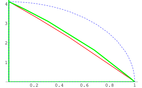
$\sigma_{p}\rightarrow 5.0\times 10^{-3}$ pb $\sigma_{n}\rightarrow 5.0\times 10^{-3}$ pb $\sigma_{p}\rightarrow 5.0\times 10^{-3}$ pb

Figure 10: The same as in Fig. 9 for the $\sigma_{p},\sigma_{n}$ plane. On the left the allowed region is that below the curve (the amplitudes are relatively real and have the same sign) . In the plots on the right the amplitudes are relatively real and of opposite sign. The allowed region is i) between the higher segment of the hyperbola and the straight line and ii) Between the straight line and the lower segment of the curve. The nuclear ME employed were those of Ressel and Dean (see table 1)

$\sigma_{n}\rightarrow 5.0\times 10^{-3}$ pb

$\sigma_{p}\rightarrow 5.0\times 10^{-3}$ pb

Figure 11: The same as in Fig. 10 assuming that the amplitudes are not relatively real, but are characterized by a phase difference $\delta$. The allowed space is now confined. The results shown for the thin solid, thick solid and dashed curves correspond to $\delta=\pi/3,~{}\pi/6$ and $\pi/2$ respectively .

VII.2 Spin matrix elements of opposite sign and $|\Omega_{p}|\gg|\Omega_{n}|$

This situation occurs in the case of the target ${}^{19}F$. As we have already mentioned the corresponding spin matrix elements shown in 1 are quite reliable. The obtained results are shown in Figs 12-14

$a_{n}\rightarrow 0.3$

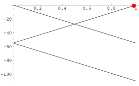
$a_{p}\rightarrow 0.3$ $a_{n}\rightarrow 0.3$ $a_{p}\rightarrow 0.3$

Figure 12: The same as in Fig. 9 for the target ${}^{19}F$. The matrix elements employed are those of table 1. Since now the proton and neutron spin ME have opposite signs, the conclusions about the relative sign of the elementary amplitudes $a_{p},a_{n}$ are opposite of those arrived in Fig. 9. The limit extracted on the neutron amplitude is poor, since the neutron spin ME is tiny.

$\sigma_{n}\rightarrow 2.3\times 10^{-3}$ pb

$\sigma_{p}\rightarrow 2.3\times 10^{-3}$ pb $\sigma_{n}\rightarrow 2.3\times 10^{-3}$ pb $\sigma_{p}\rightarrow 2.3\times 10^{-3}$ pb

Figure 13: The same as in Fig. 10 for ${}^{19}F$ with remarks about the signs of the elementary amplitudes as in Fig. 12. The matrix elements employed are those of table 1.

$\sigma_{n}\rightarrow 2.3\times 10^{-3}$ pb

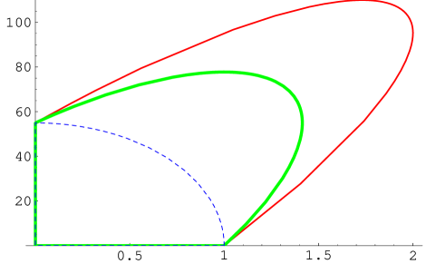
$\sigma_{p}\rightarrow 2.3\times 10^{-3}$ pb

Figure 14: The same as in Fig. 11 for ${}^{19}F$ with remarks about the signs of the elementary amplitudes as in Fig. 12. Note that now that the spin matrix elements are of opposite sign the extracted limits on the nucleon cross section are factor of two larger than assuming only one amplitude.

VII.3 Spin matrix elements of the same sign and $\Omega_{n}\gg\Omega_{p}$

This situation occurs in the case of the target ${}^{73}Ge$ (see table 1). The obtained results are shown in Figs 15-17. Now the most stringent limit is imposed on the neutron cross section.

$a_{n}\rightarrow 200$

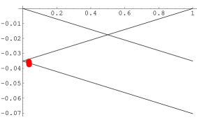
$a_{p}\rightarrow 200$ $a_{n}\rightarrow 200$ $a_{p}\rightarrow 200$

Figure 15: The same as in Fig. 9 for the target ${}^{73}Ge$. The matrix elements employed are those of table 1. The proton and neutron spin ME have the same sign, but now $\Omega_{n}\gg\Omega_{p}$. Thus the limit on $a_{n}$ is more stringent than that on $a_{p}$.

$\sigma_{n}\rightarrow 1.6$ pb

$\sigma_{p}\rightarrow 1.6$ pb $\sigma_{n}\rightarrow 1.6$ pb $\sigma_{p}\rightarrow 1.6$ pb

Figure 16: The same as in Fig. 10 for ${}^{73}Ge$ with similar remarks about the nucleon cross sections as in Fig. 15 for the amplitudes. The matrix elements employed are those of table 1.

$\sigma_{n}\rightarrow 1.6$ pb

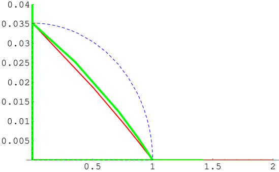
$\sigma_{p}\rightarrow 1.6$ pb

Figure 17: The same as in Fig. 11 for ${}^{73}Ge$ with remarks about the nucleon cross sections signs as in Fig. 16.

VII.4 Spin matrix elements of opposite sign and $|\Omega_{n}|\gg|\Omega_{p}|$

This situation occurs in the case of the target ${}^{3}He$. The quantities $t$ and $h$ are essentially independent of the LSP mass, since the LSP is expected to be much heavier than the nuclear mass. We find $t=2.33$ and $h=0.045$ as the modulation amplitude. The latter is a bit larger than in heavier nuclei. This means that $c_{spin}(3,\mu_{r}(3))=3t=7.00$. Likewise the parameters $\sigma_{bound}(3)~{},~{}r(m_{\chi},3)$ are also constants, $\sigma_{bound}(3)=$, $r(m_{\chi},3)=1$. Thus the expected rate is expected a bit smaller. This nucleus, however, has definite experimental advantages Santos . Furthermore the nuclear matrix elements can be calculated very reliably. The differential tate is also independent of the LSP mass. Thus it can simply be exhibited in the form:

$$\frac{dR}{du}=RL(u)\left[1+H(u)\cos{\alpha}\right]$$ (26)

Where $L(u)$, integrated from $0$ to $u_{max}=1$ yields unity, and $H(u)$ is the ratio of the modulated by the unmodulated differential rate. The situation is shown in Fig. 18.

$Q\rightarrow 26$ keV.

Figure 18: The quantities $L(u)$ (continuous curve) and $H(u)$ (dashed curve), as functions of the dimensionless energy transfer $u$, $Q=Q_{0}u$, $Q_{0}=26$ keV. For their definition see Eq. 26.

The constraints on the elementary amplitudes and the nucleon spin cross sections are shown in Figs 19-21. Again the most stringent limit is imposed on the neutron cross section.

$a_{n}\rightarrow 88$

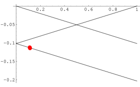
$a_{p}\rightarrow 88$ $a_{n}\rightarrow 88$ $a_{p}\rightarrow 88$

Figure 19: The same as in Fig. 15 for the target ${}^{3}He$, except that the spin matrix elements have opposite sign (now $|\Omega_{n}|>>\Omega_{p}$). As a result the inferred relative sign of the amplitudes is opposite to those of Fig.15. The matrix elements employed are those of table 1.

$\sigma_{n}\rightarrow 0.68$ pb

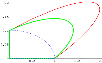
$\sigma_{p}\rightarrow 0.68$ pb $\sigma_{n}\rightarrow 0.68$ pb $\sigma_{p}\rightarrow 0.68$ pb

Figure 20: The same as in Fig. 16 for ${}^{3}He$ with the same remarks about the nucleon cross sections as in Fig. 15. The matrix elements employed are those of table 1.

$\sigma_{n}\rightarrow 0.68$ pb

$\sigma_{p}\rightarrow 0.68$ pb

Figure 21: The same as in Fig. 11 for ${}^{3}He$ with remarks about the signs of the elementary amplitudes as in Fig. 20. Note that the extracted limits are a factor of two larger than assuming only one amplitude.

VIII Conclusions

In the present paper we have studied the contribution of the axial current to the direct detection of the SUSY dark matter focusing on the popular targets ¹²⁷I, ⁷³Ge, ¹⁹F and ³He. The nuclear structure of these targets seems to favor one component, either neutron, $|\Omega_{n}|\gg|\Omega_{p}|$, or proton, $|\Omega_{p}|\gg|\Omega_{n}|$ (see table 1) . The real question is the size and the relative importance of the elementary amplitudes $a_{p}$ and $a_{n}$. These result from the combination of two factors:

• The relevant amplitudes at the quark level.
  In the case Z-exchange the the isoscalar amplitude is zero. In the case of the s-quark exchange the relative importance of the two amplitudes depends on the details of the SUSY parameter space. A priori there is no reason to prefer one amplitude over the other.

• Going from the quark to the nucleon level.
  The structure of the nucleon tends to favor the isovector component. Thus, barring unusual circumstances at the quark level, the amplitudes $a_{p}$ and $a_{n}$ have opposite sign. Unfortunately none of the nuclear systems considered satisfies the most favorable condition $\Omega_{n}=-\Omega_{p}$. Nonetheless in this case one will be able to simply extract the amplitudes $a_{p}$ and $a_{n}$ from the experimental data, if and when they become available.

In the most general case the extraction of the elementary amplitudes from the data is not going to be trivial. One can only make exclusion plots in the two dimensional ($a_{p}$, $a_{n}$) and ($\sigma_{p}$, $\sigma_{p}$) planes. By comparing such plots involving various targets one may be able to extract both amplitudes. In this work we have drawn such plots, using as input the nuclear spin response functions ( static spin ME and the relevant form factors obtained in the context of the shell model) in conjunction with the experimental limit, taken to be $\prec 16$ events per kg-y for all targets considered.

References

-
(1)
S. Hanary et al: Astrophys. J. 545, L5 (2000);
J.H.P Wu et al: Phys. Rev. Lett. 87, 251303 (2001);
M.G. Santos et al: Phys. Rev. Lett. 88, 241302 (2002). -
(2)
P.D. Mauskopf et al: Astrophys. J. 536, L59 (2002);
S. Mosi et al: Prog. Nuc.Part. Phys. 48, 243 (2002);
S.B. Ruhl al, astro-ph/0212229 and references therein. -
(3)
N.W. Halverson et al: Astrophys. J. 568, 38 (2002)
L.S. Sievers et al: astro-ph/0205287 and references therein. - (4) G. Smoot et al (COBE Collaboration): Astrophys. J. 396, L1 (1992).
- (5) D. Spergel et al: Astrophys. J. Suppl. 148, 175 (2003).
- (6) M. Tegmark et al: Phys.Rev. D 69, 103501 (2004).
- (7) A. Jaffe et al: Phys. Rev. Lett. 86, 3475 (2001).
- (8) D. Bennett et al.: Phys. Rev. Lett. 74, 2967 (1995).
- (9) R. Bernabei et al: Phys. Lett. B 389, 757 (1996).
- (10) R. Bernabei et al: Phys. Lett. B 424, 195 (1998).
-
(11)
A. Benoit et al, [EDELWEISS collaboration]: Phys. Lett. B 545, 43
(2002);
V. Sanglar,[EDELWEISS collaboration] arXiv:astro-ph/0306233;
D.S. Akerib et al,[CDMS Collaboration]: Phys. Rev D 68, 082002 (2003); arXiv:astro-ph/0405033. - (12) G. Jungman, M. Kamionkowski, and K. Griest: Phys. Rep. 267, 195 (1996).
- (13) M. W. Goodman and E. Witten: Phys. Rev. D 31, 3059 (1985).
- (14) J. Ellis and L. Roszkowski: Phys. Lett. B 283, 252 (1992).
-
(15)
A. Bottino et al., Phys. Lett B 402, 113 (1997).
R. Arnowitt. and P. Nath, Phys. Rev. Lett. 74, 4952 (1995); Phys. Rev. D 54, 2394 (1996); hep-ph/9902237;
V.A. Bednyakov, H.V. Klapdor-Kleingrothaus and S.G. Kovalenko, Phys. Lett. B 329, 5 (1994). - (16) U. Chattopadhyay and D. Roy: Phys. Rev. D 68, 033010 (2003); hep-ph/0304108.
- (17) B. Murakami and J. Wells: Phys. Rev. D 015001 (2001); hep-ph/0011082.
- (18) J. D. Vergados: J.Phys. G 30, 1127 (2004).
- (19) J. Ellis, K. A. Olive, Y. Santoso, and V. C. Spanos: Phys.Rev. D 70, 055005 (2004).
- (20) J. Hisano, S. Matsumoto, M. M. Nojiri, and O. Saito: Phys.Rev. D 71, 015007 (2005).
- (21) Update on the Direct Detection of Supersymmetric Dark Matter J. Ellis, K. A. Olive, Y. Santoso, V.C. Spanos, hep-ph/0502001.
- (22) H. Ejiri, K. Fushimi, and H. Ohsumi: Phys. Lett. B 317, 14 (1993).
- (23) J. Vergados, P.Quentin, and D. Strottman: IJMPE 14, 751 (2005).
- (24) D. Santos et al, The MIMAC-He3 Collaboration, A New 3He Detector for non Baryonic Dark Matter Search, Invited talk in idm2004 (to appear in the proceedings).
- (25) T. Kosmas and J. Vergados: Phys. Rev. D 55, 1752 (1997).
- (26) J. D. Vergados: J. of Phys. G 22, 253 (1996).
- (27) M. Drees and N. N. Nojiri, Phys. Rev. D 48, 3843 (1993); Phys. Rev. D 47, 4226 (1993).
- (28) T.P. Cheng, Phys. Rev. D 38, 2869 (1988); H-Y. Cheng, Phys. Lett. B 219, 347 (1989).
- (29) M.T. Ressell et al., Phys. Rev. D 48, 5519 (1993); M.T. Ressell and D.J. Dean, Phys. Rev. C 56, 535 (1997).
- (30) P. C. Divari, T. Kosmas, J. D. Vergados, and L. Skouras: Phys. Rev. C 61, 044612 (2000).
- (31) K. F. A. K. Drukier and D. N. Spergel: Phys. Rev. D 33, 3495 (1986).
- (32) K. Frese, J. A. Friedman, and A. Gould: Phys. Rev. D 37, 3388 (1988).
- (33) J. Vergados: Phys. Rev. D 58, 103001 (1998).
- (34) J. D. Vergados: Phys. Rev. D 63, 06351 (2001).
- (35) J. I. Collar et al: Phys. Lett. B 275, 181 (1982).
- (36) J. D. Vergados: Phys. Rev. Lett. 83, 3597 (1999).
- (37) P. Ullio and M. Kamioknowski: JHEP 0103, 049 (2001).
- (38) A. Green: Phys. Rev. D 66, 083003 (2002).
- (39) J. D. Vergados: Part. Nucl. Lett. 106, 74 (2001); hep-ph/0010151.
- (40) K.N. Buckland, M.J. Lehner and G.E. Masek, in Proc. 3nd Int. Conf. on Dark Matter in Astro- and part. Phys. (Dark2000), Ed. H.V. Klapdor-Kleingrothaus, Springer Verlag (2000).
-
(41)
M.E.Gómez and J.D. Vergados, Phys. Lett. B 512 , 252 (2001);
hep-ph/0012020.
M.E. Gómez, G. Lazarides and Pallis, C., Phys. Rev.D 61, 123512 (2000) and Phys. Lett. B 487, 313 (2000). - (42) A. Arnowitt and B. Dutta, Supersymmetry and Dark Matter, hep-ph/0204187.
- (43) U. Chattopadhyay, A. Corsetti, and P. Nath: Phys. Rev. D 68, 035005 (2003).
- (44) The Strange Spin of the Nucleon, J. Ellis and M. Karliner, hep-ph/9501280.
- (45) E. Homlund and M. Kortelainen and T.S. Kosmas and J. Suhonen and J. Toivanen, Phys. Lett B, 584,31 (2004); Phys. Atom. Nucl. 67, 1198 (2004).
- (46) E. Moulin, F. Mayet, and D. Santos: Phys. Lett. B 614, 143 (2005).
- (47) J. D. Vergados: Phys. Rev. D 62, 023519 (2000).
- (48) Dark Matter Candidates in Supersymmetric Models K. A. Olive, Summary of talk at Dark 2004, proceedings of 5th International Heidelberg Conference on Dark Matter in Astro and Particle Physics, hep-ph/0412054.
- (49) D. S. Akerib et al (CDMS Collaboration): Phys.Rev.Lett. 93, 211301 (2004).
- (50) C. Savage, P. Gondolo, and K. Freese: Phys. Rev. D 70, 123513 (2004).
- (51) F. Giuliani and T. Girard: Phys.Lett. B 588, 151 (2004).