Supersymmetry Simulations with Off-Shell Effects
for LHC and ILC

ABSTRACT

At the LHC and at an ILC, serious studies of new physics benefit from a proper simulation of signals and backgrounds. Using supersymmetric sbottom pair production as an example, we show how multi-particle final states are necessary to properly describe off-shell effects induced by QCD, photon radiation, or by intermediate on-shell states. To ensure the correctness of our findings we compare in detail the implementation of the supersymmetric Lagrangian in madgraph, sherpa and whizard. As a future reference we give the numerical results for several hundred cross sections for the production of supersymmetric particles, checked with all three codes.

1 Introduction

The discoveries of the electroweak gauge bosons and the top quark more than a decade ago established perturbative quantum field theory as a common description of electromagnetic, weak, and strong interactions, universally applicable for energies above the hadronic ${\rm GeV}$ scale. The subsequent measurements of QCD and electroweak observables in high-energy collision experiments at the SLAC SLC, CERN LEP, and Fermilab Tevatron have validated this framework to an unprecedented precision. Nevertheless, the underlying mechanism of electroweak symmetry breaking remains undetermined. It is not clear how the theory should be extrapolated beyond the electroweak scale $v=246\;{\rm GeV}$ to the ${\rm TeV}$ scale or even higher energies [1].

At the LHC (and an ILC) this energy range will be directly probed for the first time. If the perturbative paradigm holds, we expect to see fundamental scalar Higgs particles, as predicted by the Standard Model (SM). Weak-scale supersymmetry (SUSY) is a leading possible solution to theoretical problems in electroweak symmetry breaking, and predicts many additional new states. The minimal supersymmetric extension of the Standard Model (MSSM) is a model of softly-broken SUSY. The supersymmetric particles (squarks, sleptons, charginos, neutralinos and the gluino) can be massive in comparison to their SM counterparts. Previous and current high-energy physics experiments have put stringent lower bounds on supersymmetric particle masses, while fine-tuning arguments lead us to believe they do not exceed a few ${\rm TeV}$. Therefore, a discovery in Run II at the Tevatron is not unlikely [2], and it will fall to the LHC to perform a conclusive search for SUSY, starting in 2008. Combining the energy reach of the LHC with precision measurements at a possible future electron-positron collider ILC, a thorough quantitative understanding of the SUSY particles and interactions would be possible [3].

Most realistically, SUSY will give us a plethora of particle production and decay channels that need to be disentangled and separated from the SM background. To uncover the nature of electroweak symmetry breaking we not only have to experimentally analyze multi-particle production and decay signatures, we also need to accurately simulate the model predictions on the theory side.

Much SUSY phenomenology has been performed over the years in preparation for LHC and ILC, nearly all of it based on relatively simple $2\to 2$ processes [4, 5] or their next-to-leading order (NLO) corrections. These approximations are useful for highly inclusive analyses and convenient for analytical calculations, but should be dropped once we are interested in precise measurements and their theoretical understanding. Furthermore, for a proper description of data, we need Monte-Carlo event generators that fully account for high-energy collider environments. Examples for necessary improvements include: consideration of spin correlations [28] and finite width effects in supersymmetric particle decays [65]; SUSY-electroweak and Yukawa interferences to some SUSY-QCD processes; exact rather than common virtual squark masses; and $2\to 3$ or $2\to 4$ particle production processes such as the production of hard jets in SUSY-QCD processes [6] or SUSY particles produced in weak-boson fusion (WBF) [7].

In this paper we present three new next-generation event generators for SUSY processes: madgraph ii/madevent [8, 9], o’mega/whizard [10, 11], and amegic++/sherpa [12, 13]. They properly take into account various physics aspects which are usually approximated in the literature, such as those listed above. They build upon new methods and algorithms for automatic tree-level matrix element calculation and phase space generation that have successfully been applied to SM phenomenology [14, 15, 16]. Adapted to the more involved structure of the MSSM, they are powerful tools for a new round of MSSM phenomenology, especially at hadron colliders.

The structure of the paper is as follows: In Sec. 2 we consider basic requirements for realistic SUSY simulations, in particular the setup of consistent calculational rules and conventions as a conditio sine qua non for obtaining correct and reproducible results. Sec. 3 gives some details of the implementation of MSSM multi-particle processes in the three generators, while Sec. 4 is devoted to numerical checks. Finally, Secs. 5 and 6 cover one particular application, the physics of sbottom squarks at the LHC and an ILC, respectively. Our emphasis lies on off-shell effects of various kinds which for the first time we accurately describe using the tools presented in this paper.

In the extensive Appendix we list as a future reference cross sections for several hundred SUSY $2\to 2$ processes that are the main part of these checks. We include all information necessary to reproduce these numbers.

2 Supersymmetry Simulations

Throughout this paper, we assume R-parity conservation in the MSSM. The SUSY particle content consists of the SM particles, the five Higgs bosons, and their superpartners, namely six sleptons, three sneutrinos, six up-type and six down-type squarks, two charginos, four neutralinos, and the gluino. We allow for a general set of TeV-scale (or weak-scale) MSSM parameters, with a few simplifying restrictions: (i) we assume CP conservation, i.e. all soft-breaking terms in the Lagrangian are real (cf. also (iii) below); (ii) we neglect masses and Yukawa couplings for the first two fermion generations, i.e. left-right mixing occurs only for third-generation squarks and sleptons; (iii) correspondingly, we assume the SM flavor structure to be trivial, $V_{\rm CKM}=V_{\rm MNS}=1$; (iv) we likewise assume the flavor structure of SUSY-breaking terms to be trivial.

None of these simplifications is a technical requirement, and all codes are capable of dealing with complex couplings as well as arbitrary fermion and sfermion mass and mixing matrices. However, with very few exceptions, these effects are numerically unimportant or irrelevant for the simulation of SUSY scattering and decay processes at high-energy colliders. (In Sec. 4.3 we discuss residual effects of nontrivial flavor structure.)

We thus define the MSSM as the general TeV/weak-scale Lagrangian for the SM particles with two Higgs doublets, with gauge- and Lorentz-invariant, R-parity-conserving, renormalizable couplings, and softly-broken supersymmetry. Unfortunately, while this completely fixes the physics, it leaves a considerable freedom in choosing phase conventions. The large number of Lagrangian terms leaves ample room for error in deriving Feynman rules, coding them in a computer program, and relating the input parameters to a standard convention.

The three codes we consider here are completely independent in their derivation of Feynman rules, implementation, matrix element generation, phase space setup, and integration methods. A detailed numerical comparison should therefore reveal any mistake in these steps. To this end, we list a set of $2\to 2$ scattering processes that involve all Feynman rules that could be of any relevance in Sec. 4.

2.1 Parameters and Conventions

Apart from the simplifications listed above, we do not make any assumptions about SUSY breaking. No physical parameters are hard-coded into the programs. Instead, all codes use a set of weak-scale parameters in the form of a SUSY Les Houches Accord (SLHA) input file [17]. This file may be generated by any one of the standard SUSY spectrum generators [18, 19].

Since the SLHA defines weak-scale parameters in a particular renormalization scheme, we have to specify how to use them for our tree-level calculations: we fix the electroweak parameters via $G_{F}$, $M_{Z}$, and $\alpha_{\rm QED}$. Using the tree-level relations (as required for gauge-invariant matrix elements at tree level) we obtain parameters such as $\sin^{2}\theta_{w}$ and $M_{W}$ as derived quantities; $M_{W}$ and $M_{Z}$ are defined as pole masses.

The SLHA uses pole masses for all MSSM particles, while mixing matrices and Yukawa couplings are given as loop-improved $\overline{\rm DR}$ values. From this input we need to derive a set of mass and coupling parameters suitable for comparing tree-level matrix-element calculations. This leads to violation of electroweak gauge invariance which we discuss in Sec. 2.2. However, numerically this is a minor problem, relevant only for some processes (e.g. SUSY particle production in weak-boson fusion [7]) at asymptotically high energies. For the numerical results of this paper, we therefore use the SLHA masses and mixing matrices at face value.

For the bottom and top quarks we identify the (running) Yukawa couplings and the masses, as required by gauge invariance. The weak scale as the renormalization point yields realistic values for the Yukawa couplings. One might be concerned that the kinematical masses are then off from their actual values. However, since our production cross section should be regarded as the leading contribution to the inclusive cross section, the relevant scale is the energy scale of the whole process rather than the scale of individual heavy quarks. This necessitates the use of running masses to make a reliable estimate.

The trilinear couplings and the $\mu$ parameter which explicitly appear in some couplings are fixed by the off-diagonal entries in the chargino, neutralino and sfermion mass matrices. We adopt two schemes for negative neutralino mass eigenvalues: sherpa and madgraph use the negative values directly in the propagator and wave function. o’mega/whizard rotates the neutralino fields to positive masses, which yields a complex neutralino mixing matrix, even though CP is conserved.

For our comparison we neglect all couplings that contain masses of light-flavor fermions, i.e. the Higgs couplings to first- and second-generation fermions and their supersymmetric counterparts; as well as left–right sfermion mixing. This includes neglecting light fermion masses in the neutralino and chargino sector, which would otherwise appear via Yukawa-higgsino couplings. Physically, this is motivated by flavor constraints which forbid large deviations from universality in the first and second generations [20]. For our LHC calculations we employ CTEQ5 parton distribution functions [21].

2.2 Unitarity and the SLHA Convention

The MSSM is a renormalizable quantum field theory [22]. To any fixed order in perturbation theory, a partial-wave amplitude calculated from the Feynman rules, renormalized properly, is bounded from above. Cross sections with a finite number of partial waves (e.g. $s$-channel processes) asymptotically fall off like $1/s$, while massless particle exchange must not lead to more than a logarithmic increase with energy. This makes unitarity a convenient check for the Feynman rules in our matrix element calculators.

As an example, individual diagrams that contribute to $2\to 2$ weak boson scattering rise like the fourth power of the energy, but the two leading terms of the energy expansion cancel among diagrams to ameliorate this to a constant. This property connects the three- and four-boson vertices, and predicts the existence and couplings of a Higgs boson, assuming the theory is weakly interacting to high energies [23]. For example, for weak boson fusion to neutralinos and charginos, these unitarity cancellations can be neatly summarized in a set of sum rules for the SUSY masses and couplings [7]. For generic Higgs sectors, the unitarity relations were worked out in [24].

Many, but not all, terms in the Lagrangian can be checked by requiring unitarity. For instance, gauge cancellations in $WW$ scattering to two SUSY particles need not happen if the final-state particle has an $SU(2)\times U(1)$ invariant mass term. In the softly-broken SUSY Lagrangian, this property holds for the gauginos and higgsinos as well as for the second Higgs doublet in the MSSM. For these particles, we expect unitarity relations to impose some restrictions on their couplings, but not a complete set of equations, so some couplings remain unconstrained.

As mentioned above, for our numerical comparison of SUSY processes we use a renormalization-group improved spectrum in the SLHA format [18, 19]. In particular, we adopt this spectrum for the Higgs sector, where gauge invariance (or unitarity) relates masses, trilinear and quartic couplings. While at tree-level all unitarity relations are automatically satisfied, any improved spectrum will violate unitarity constraints unless the Higgs trilinear couplings are computed in the same scheme. However, not all couplings are known to the same accuracy as the Higgs masses [25]. We follow the standard approach of computing the trilinear Higgs couplings from effective mixing angles $\alpha$ and $\beta$. As a consequence, we expect unitarity violation. Luckily, this only occurs in $2\to 3$ processes of the type $WW\to WWH$ [24], while in $2\to 2$ processes of the type $WW\to HH$ where one might naively expect unitarity violation, the values of the Higgs trilinear couplings change the value of total high-energy asymptotic cross section but do not affect unitarity.

A similar problem arises in the neutralino and chargino sector. Unitarity is violated at high energies in processes of the type $VV\to\tilde{\chi}\tilde{\chi}$ ($V=W,Z$) [7]. If we use the renormalization-group improved $\overline{\rm DR}$ neutralino and chargino mass matrices (or equivalently the masses and mixing matrices) the gaugino–higgsino mixing entries which are equivalent to the Higgs couplings of the neutralinos and the charginos implicitly involve $M_{W,Z}$, also in the $\overline{\rm DR}$ scheme. To ensure proper gauge cancellations which guarantee unitarity, these gauge boson masses must be identical to the kinematical masses of the gauge bosons in the scattering process, which are usually defined in the on-shell scheme. One possible solution would be to extract a set of gauge boson masses that satisfies all tree-level relations from the mass matrices. This scheme has the disadvantage that while it works for the leading corrections, it will likely not be possible to derive a consistent set of weak parameters in general. Moreover, the higher-order corrections included in the renormalization-group improved neutralino and chargino mass matrices will not be identical to the leading corrections to, for example, the $s$-channel propagator mass. However, an artificial spectrum that is specifically designed to fulfill the tree-level relations can be used for a technical test of high-energy unitarity. Such a detailed check has been performed for the susy-madgraph implementation [7].

2.3 Symmetries and Ward Identities

An independent method for verifying the implementation is the numerical test of symmetries and their associated Ward identities. A trivial check is provided by the permutation and crossing symmetries of many-particle amplitudes. More subtle are the Ward identities of gauge symmetries, which can be tested by replacing the polarization vector of any one external gauge boson by its momentum $\epsilon_{\mu}(k)\to k_{\mu}$ and, if necessary, subtracting the amplitude with the corresponding Goldstone boson amplitude. Finally, the SUSY Ward identities can be tested numerically.

Ward identities have the advantage that they require no additional computer program, can be constructed automatically and can be applied separately for each point in phase space. If applied in sensitive regions of phase space, tests of Ward identities will reveal numerical instabilities. Extensive tests of this kind have been carried out for the matrix elements generated by o’mega and its associated numerical library for the SM [26] and for the MSSM [27].

2.4 Intermediate Heavy States

During the initial phase of the LHC, narrow resonances can be described by simple $2\to 2$ production cross sections and subsequent cascade decays. However, establishing that these resonances are indeed the long-sought SUSY partners would call for more sophisticated tools.

The identification of resonances as SUSY partners would require determination of their spin and parity quantum numbers [28]. This in turn requires a proper description of the spin correlations among the particles in the production and the decay cascades. The simplest consistent approximation calculates the Feynman diagrams for the $2\to n$ process and forces narrow intermediate states on the mass shell without affecting spin correlations. For fermions we can write the leading term in the small expansion parameter $\Gamma/m$ as:

$$\frac{1}{|s-m+\mathrm{i}\Gamma|^{2}}\to\frac{\pi}{m\Gamma}\,\delta(s-m^{2})$$ (1)

For SM processes this computation of $2\to n$ matrix elements has been successfully automatized by the programs described below. The alternative approach of manually inserting the appropriate density matrices for production and decay is more error-prone due to the need for consistent phase conventions.

The width of the heavy resonances are themselves observables predicted by SUSY for a given set of soft breaking parameters and should be taken into account. A naïve Lorentzian smearing of Eq. (1) will not yield a theoretically consistent description of finite width effects. Gauge and SUSY Ward identities are immediately violated once amplitudes are continued off-shell. Since scattering amplitudes in gauge theories and SUSY theories exhibit strong numerical cancellations, the violation of the corresponding Ward identities can result in numerically large effects. Therefore a proper description of a resonance with a finite width requires a complete gauge invariant set of diagrams, the simplest of which is the set of all diagrams contributing to the $2\to n$ process [29]. In Secs. 5 and 6 we study the numerical impact of finite-width effects for the concrete example of sbottom production at high-energy colliders.

Intermediate charged particles with finite widths present additional gauge invariance issues, which were studied at LEP2 in great detail for $W$ boson production processes [30]. Although various prescriptions for widths are available in the matrix element generators described in the paper, we used the fixed-width scheme for the calculations. A careful analysis on the impact of different choices is beyond the scope of the paper.

3 Calculational Methods and Algorithms

Each of the three calculational tools we use for this paper consists of two independent programs. The first program uses a set of Feynman rules, which can be preset or user-defined, to generate computer code that numerically computes the tree-level scattering amplitude for a chosen process. These numerical codes call library functions to compute wave functions of external particles, internal currents and vertices to obtain the complete helicity amplitude (the amplitude for all helicity configurations of external particles, which are then summed over [31]). The second program performs adaptive phase space integration and event generation, and produces integrated cross sections and weighted or unweighted event samples. The required phase space mappings are determined automatically, using appropriate heuristics, from the ‘important’ Feynman diagrams contributing to the process that is being studied.

In principle, there is nothing that precludes the use of other combinations of the three matrix element generators and the three phase space integrators. In practice however, it requires some effort to adopt the interfaces that have grown organically. Nevertheless, whizard can e.g. use madgraph as an alternative to o’mega.

helas [32] is the archetypal helicity amplitude library and is now employed by many automated matrix element generators. The elimination of common subexpression to optimize the numerical evaluation was already suggested in Refs. [32] for the manual construction of scattering amplitudes. The actual libraries used by our three tools choose between different trade-offs of maintainability, extensibility, efficiency and numerical accuracy.

Majorana spinors are the crucial new ingredient for calculating helicity amplitudes in supersymmetric field theories. In the simple example process $e^{+}e^{-}\to\tilde{\chi}\tilde{\chi}$ we see the complication which arises: if we naïvely follow the fermion number flow of the incoming fermions, the $t$-channel and $u$-channel amplitudes require different external spinors for the final-state fermions. The most elegant algorithm known for unambiguously assigning a fermion flow and the relative signs among Feynman diagrams is described in Ref. [33]. Consequently, all matrix element generators use an implementation of this algorithm.

Beneath some common general features, the similarities of the three tools quickly disappear: they use different algorithms, implemented in different programming languages. That such vastly different programs can be tested against each other with a Lagrangian as complex as that of the TeV-scale MSSM should give confidence in the predictive power of these programs for SUSY physics at the LHC and later at an ILC.

To compute cross sections in the MSSM, we need a consistent set of particle masses and mixing matrices, computed for a chosen SUSY-breaking scenario. Various spectrum generators are available, all using the SUSY Les Houches Accord as their spectrum interface. The partonic events generated by our three tools can either be fragmented by a built-in algorithm (sherpa) or passed via a standard interface to external hadronization packages [34]. However, proper hadronization of the parton level results presented here is beyond the scope of this paper.

3.1 madgraph ii and madevent

madgraph [8] was the first program allowing fully automated calculations of squared helicity amplitudes in the Standard Model. In addition to being applied to many physics calculations, it was later frequently used as a benchmark for testing the accuracy of new programs as well as for gauging the improvements implemented in the new programs.

madgraph ii is implemented in fortran77. It generates all Feynman diagrams for a given process, performs the color algebra and translates the result into a fortran77 procedure with calls to the helas library. During this translation, redundant subexpressions are recognized and computed only once. While the complexity continues to grow asymptotically with the number of Feynman diagrams, this approach generates efficient code for typical applications.

The correct implementation of color flows for hadron collider physics was an important objective for the very first version of madgraph, while the implementation of extensions of the standard model remained nontrivial for users. madgraph ii reads the model information from two files and supports Majorana fermions, allowing fully automated calculations in the MSSM. The MSSM implementation makes use and extends the list of Feynman rules that have been derived in the context of [35, 36, 37].

madevent [9] uses phase space mappings based on single squared Feynman diagrams for adaptive multi-channel sampling [38]. The madgraph/madevent package has a web-based user interface and supports shortcuts such as summing over initial state partons, summing over jet flavors and restricting intermediate states. Interfaces to parton shower and hadronization Monte Carlos [34] are available.

3.2 o’mega and whizard

o’mega [10] and whizard [11] were initially designed for $e^{+}e^{-}$ linear colliders studies. o’mega constructs numerically stable and optimally factorized scattering amplitudes and allows the study of physics beyond the Standard Model. A general treatment of color was added to o’mega only recently and is currently available only in conjunction with whizard.

o’mega constructs an expression for the scattering matrix element from a description of the Feynman rules and the target programming language. The complexity of these expressions grows only exponentially with the number of external particles, unlike the factorial growth of the number of Feynman diagrams. Optionally, o’mega can calculate cascades: long-lived intermediate particles can be forced on the mass shell in order to obtain gauge invariant approximations with full spin correlations.

o’mega is implemented in the functional programming language Objective Caml [39], but the compiler is portable and no knowledge of Objective Caml is required for using o’mega with the supported models. The tables describing the Lagrangians can be extended by users. Its set of MSSM Feynman rules was derived in accordance with Ref. [40].

whizard builds a Monte Carlo event generator on the library VAMP [41] for adaptive multi-channel sampling. It uses heuristics to construct phase space parameterizations corresponding to the dominant time- and space-like singularities for each process. For processes with many identical particles in the final state, symmetries are used extensively to reduce the number of independent channels.

whizard is written in fortran95, with some Perl glue code. It is particularly easy to simulate multiple processes (i.e. reducible backgrounds) with the correct relative rates simultaneously. It has an integrated interface to pythia [42] that follows the Les Houches Accord [34] for parton showers and hadronization.

3.3 amegic++ and sherpa

sherpa [13] is a new complete Monte Carlo Generator for collider physics, including hard matrix elements, parton showers, hadronization and other soft physics aspects, written from scratch in C++. The key feature of sherpa is the implementation of an algorithm [43, 44, 45], which allows consistent combination of tree-level matrix elements for the hard production of particles with the subsequent parton showers that model softer bremsstrahlung. This algorithm has been tested in various processes [46, 47]. Both of the other programs described above connect their results with full event simulation through interfaces to external programs.

amegic++ [12] is the matrix element generator for sherpa. It generates all Feynman diagrams for a process from a model description in C++. Before writing the numerical code to evaluate the complete amplitude (including color flows), it eliminates common subexpressions. En passant, it selects appropriate phase space mappings for multi-channel sampling and event generation [38]. For integration it relies on vegas [48] to further improve the efficiency of the dominant integration channels. The MSSM Feynman rules and conventions in amegic++ are taken from Ref. [49].

4 Pair Production of SUSY Particles

4.1 The Setup

As long as R-parity is conserved, SUSY particles are only produced in pairs. Therefore, SUSY phenomenology at the LHC and ILC amounts to essentially searching for all accessible supersymmetric pair-production channels with subsequent (cascade) decays. Proper simulations need to describe this type of processes as accurately as possible. This requires a careful treatment of many-particle final states, off-shell effects and SUSY as well as SM backgrounds. The complexity of this task and the variety of conventions and schemes commonly used require careful cross-checks at all levels of the calculation.

As a first step, we present a comprehensive list of total cross sections for on-shell supersymmetric pair production processes (cf. Appendix B). These results give a rough overview of the possible SUSY phenomenology at future colliders, at least for the chosen point in SUSY parameter space. The second purpose of this computation is a careful check of our sets of Feynman rules and their numerical implementation. After testing our tools we will then move on to a proper treatment beyond naïve $2\to 2$ production processes. We compute all numbers independently with madgraph, whizard, and sherpa, using identical input parameters. We adopt a MSSM parameter set that corresponds to the point SPS1a [50]. This point assumes gravity mediated supersymmetry breaking with the universal GUT-scale parameters:

$$m_{0}=100\;{\rm GeV}\;,\qquad m_{1/2}=250\;{\rm GeV}\;,\qquad A_{0}=-100\;{\rm GeV}\;,\qquad\tan\beta=10\;,\qquad\mu>0\;.$$ (2)

We use softsusy to compute the TeV-scale physical spectrum [18]. For the purpose of evaluating $2\to 2$ cross sections, we set all SUSY particle widths to zero. The final states are all possible combinations of two SUSY partners or two Higgs bosons. The initial states required to test all the SUSY vertices are:

$$e^{+}e^{-},\ e^{-}\bar{\nu}_{e},\ e^{-}e^{-},\ \tau^{+}\tau^{-},\ \tau^{-}\bar{\nu}_{\tau},\ u\bar{u},\ d\bar{d},\ uu,\ dd,\ b\bar{b},\ b\bar{t},\$$

$$W^{+}W^{-},\ W^{-}Z,\ W^{-}\gamma,\ ZZ,\ Z\gamma,\ \gamma\gamma,\ gW^{-},\ gZ,\ g\gamma,\ gg,\ ug,\ dg\,.$$

The (partonic) initial-state energy is always fixed. This allows for a comparison of cross sections without dependence on parton structure functions, and with much-improved numerical efficiency. Clearly, some of these initial states cannot be realized on-shell or are even impossible to realize at a collider. They serve only as tests of the Feynman rules. Any MSSM Feynman rule relevant for an observable collider process is involved in at least one of the considered processes. For SM processes, comprehensive checks and comparisons were performed in the past [51].

The complete list of input parameters is given in Appendix A. The input is specified in the SLHA format [17]. This ensures compatibility of the input conventions, even though different conventions for the Lagrangian and Feynman rules are used by the different programs.

In Appendix B, we list and compare the results for two partonic c.m. energies $\sqrt{s}=500\;{\rm GeV}$ and $2\;{\rm TeV}$. All results agree within a Monte Carlo statistical uncertainty of $0.1\%$ or less. These errors reflect neither the accuracy nor the efficiency of any of the programs; we do not specify the number of matrix element calls or the amount of CPU time required in the computation. To obtain a precise $2\to 2$ total cross section, Monte Carlo integration is not a good choice. On the other hand these simple processes serve as the most efficient framework to test the numerical implementation of Feynman rules and the MSSM spectrum.

We emphasize that the three programs madgraph, whizard, and sherpa, and their SUSY implementation are completely independent. As explained in Sec. 3, they use different conventions, signs and phase choices for the MSSM Feynman rules; have independent algorithms and helas-type libraries; and use different methods for parameterizing and sampling the phase space. We consider our results a strong check that covers all practical aspects of MSSM calculations, from the model setup to the numerical details. Specifically, we confirm the Feynman rules in Ref. [49] as they are used in sherpa. These Feynman rules do not use the SLHA format, so translating them is a non-trivial part of the implementation. For madgraph and whizard, the Feynman rules were derived independently.

4.2 Sample Cross Sections

We briefly discuss our cross section results and their physical interpretation. While the numbers are specific for the chosen point SPS1a [50] and its associated mass spectrum, many features of the results are rather generic in one-scale SUSY breaking models and depend only on the structure of the TeV-scale MSSM.

4.2.1 $\mathbf{e^{+}e^{-}}$ processes

All $e^{+}e^{-}$–induced SUSY production cross sections receive contributions from $s$-channel $Z$ and (for charged particles) photon exchange. The couplings of the supersymmetric particles to $Z$ and photon are determined by the $SU(2)_{L}\times U(1)_{Y}$ gauge couplings and mixing angle. As expected from perturbative unitarity, all $s$-channel-process cross sections asymptotically fall off like $1/s$. If the process in question includes $t$-channel exchange, then we must sum over all partial waves

$$\frac{m^{2}}{2p\cdot k+m^{2}}\;=\;\sum^{\infty}_{n=0}\biggl{(}\frac{-2p\cdot k}{m^{2}}\biggr{)}^{n}\Longrightarrow\quad\sigma\propto\frac{1}{s}\times\begin{cases}\log\frac{s}{m^{2}}&\text{for no vector boson exchange,}\\ \phantom{\log}\frac{s}{m^{2}}&\text{for vector boson exchange.}\end{cases}$$ (3)

The implication of the second line is that Coulomb scattering, WBF, and in some sense all hadronic cross sections, do not decrease with $s$.

We show the $e^{+}e^{-}$ cross sections in Table B.1. The largest, of up to a few hundred fb at $\sqrt{s}=500\;{\rm GeV}$, correspond to sneutrino and selectron production, $\tilde{\chi}^{0}_{1}$ and $\tilde{\chi}^{0}_{2}$, and chargino pair production. These are the processes with a dominant $t$-channel slepton contribution. In SPS1a the heavier neutralinos $\tilde{\chi}^{0}_{3},\tilde{\chi}^{0}_{4}$ are almost pure higgsinos. Higgsinos couple only to the $s$-channel $Z$, and diagonal pair production of $\tilde{\chi}^{0}_{3}\tilde{\chi}^{0}_{3},\tilde{\chi}^{0}_{4}\tilde{\chi}^{0}_{4}$ is suppressed because of the inherent cancellation between the two higgsino fractions $h_{u}$ and $h_{d}$; i.e. the amplitudes are proportional to $|h_{u}|^{2}-|h_{d}|^{2}$, which vanishes in the limit where they have the same higgsino masses. Only mixed $\tilde{\chi}^{0}_{3}\tilde{\chi}^{0}_{4}$ production has a significant cross section, because it is proportional to the sum $|h_{u}|^{2}+|h_{d}|^{2}$.

In the Higgs sector, SPS1a realizes the decoupling limit where the light Higgs $h$ closely resembles the SM Higgs. The production channels $Zh$, $AH$, and $H^{+}H^{-}$ dominate if kinematically accessible, while the reduced coupling of the $Z$ to heavy Higgses strongly suppresses the $ZH$ and $Ah$ channels.

For completeness, we also show the $e^{-}\bar{\nu}_{e}$ set of cross sections in Table B.3, even though such a collider is infeasible.

4.2.2 $\mathbf{W^{+}W^{-}}$ and $\mathbf{WZ}$ processes

The cross sections for weak boson fusion processes, shown in Tables B.6 and B.7, are generically of the same order of magnitude as their fermion-initiated counterparts, with a few notable differences. In addition to gauge boson exchange, $s$- and $t$-channel Higgs exchange contributes to WBF production of third-generation sfermions, neutralinos, charginos, and Higgs/vector bosons. These processes are sensitive to a plethora of Higgs couplings to supersymmetric particles. Furthermore, the longitudinal polarization components of the external vector bosons approximate, in the high-energy limit, the pseudo-Goldstone bosons of electroweak symmetry breaking. This results in a characteristic asymptotic behavior (that can be checked by inserting $\sqrt{s}$ values of several ${\rm TeV}$, not shown in the tables): the total cross sections for vector-boson and CP-even Higgs pair production in WBF approach a constant at high energy, corresponding to $t$-channel gauge boson exchange between two scalars. Production cross sections that contain the CP-odd Higgs or the charged Higgs instead decrease like $1/s$, because no scalar-Goldstone-gauge boson vertices exist for these particles.

In the cases involving first and second generation sfermions, $t$-channel sfermion exchange with an initial-state $W$ contributes only to left-handed sfermions, so the $\tilde{f}_{L}\tilde{f}_{L}^{*}$ cross sections dominate over $\tilde{f}_{R}\tilde{f}_{R}^{*}$. In the neutralino sector, $\tilde{\chi}^{0}_{1}$ is dominantly bino and does not couple to neutral Higgs bosons, so $\tilde{\chi}^{0}_{1}$ production in $W^{+}W^{-}$ fusion is suppressed. The other neutralinos and charginos, being the SUSY partners of massive vector bosons and Higgses, are produced with cross sections up to $100\;{\rm pb}$. The largest neutralino rates occur for mixed gaugino and higgsino production, because the Yukawa couplings are given by the gaugino–higgsino mixing entry in the neutralino mass matrix. In the Higgs sector, the decoupling limit ensures that only $W^{+}W^{-}\to Zh$, $WZ\to Wh$ (almost $100\;{\rm pb}$), and $W^{+}W^{-}\to hh$ ($6\;{\rm pb}$) are important, while the production of heavy Higgses is suppressed. For $W^{+}W^{-}\to Ah$ and $W^{-}Z\to H^{-}h$ the decoupling suppression applies twice.

In reality, $WW\to XX$ and $WZ\to XY$ scattering occurs only as a subprocess of $2\to 6$ multi-particle production. The initial vector bosons are emitted as virtual states from a pair of incoming fermions. The measurable cross sections are phase-space suppressed by a few orders of magnitude. A rough estimate can be made by folding the energy-dependent $WW/WZ$ cross sections with weak-boson structure functions. Reliable calculations require the inclusion of all Feynman diagrams, as can be done with the programs presented in this paper — the production rates rarely exceed ${\cal O}({\rm ab})$ at the LHC [7].

4.2.3 Other processes

For the remaining lists of processes with vector-boson or fermion initial states, similar considerations apply. In particular, the photon has no longitudinal component, so $\gamma$-induced electroweak processes (Tables B.8, B.10 and B.11) are not related to Goldstone-pair scattering. We include unrealistic fermionic initial states such as $\tau^{+}\tau^{-}$, $\tau^{-}\bar{\nu_{\tau}}$ and $b\bar{t}$ in our reference list, Tables B.2, B.4 and B.5, because they involve Feynman rules that do not occur in other production processes, but are relevant for decays.

Finally, our set of processes contains several lists with the colored fermionic initial states $u\bar{u}$, $d\bar{d}$ and $b\bar{b}$ (Tables B.16–B.18, plus Table B.20 for same-flavor fermions); $gg$-fusion (Table B.15); $qg$-fusion (Table B.19); and mixed QCD-electroweak processes $gA$, $gZ$ and $gW$ (Tables B.12, B.13 and B.14). These (as full hadronic processes) are accessible at hadron colliders, and comparing their cross sections completes our check of Feynman rules of the SUSY-QCD sector and its interplay with the electroweak interactions. Note that for a transparent comparison we do not fold the quark- and gluon-induced processes with structure functions.

The only Feynman rules not checked by any process in this list are the four-scalar couplings. It is expected, and has explicitly been verified for the four-Higgs coupling in particular [52], that these contact interactions are not accessible at any collider in the foreseeable future. We therefore neglect them.

4.3 Flavor Mixing

For most of this paper we have neglected the quark masses and the mixings of the first two squark and slepton/sneutrino generations. Here we give a brief account of the consequences of using a non-diagonal CKM matrix. Full CKM mixing is available as an option for the whizard and sherpa event generators. For madgraph, it is straightforward to modify the model definition file accordingly.

The CKM mixing matrix essentially drops out from most processes when we sum over all quark intermediate and final states. This is due to CKM unitarity, violated only by terms proportional to the quark mass squared over $\sqrt{s}$ in high energy scattering processes. For the first two generations, such corrections are negligible at the energies we are considering.

At hadron colliders, summation over initial-state flavors does not lead to cancellation because the parton densities are flavor-dependent. In the SM, CKM structure matters only for charged-current processes where a $q\bar{q}^{\prime}$ pair annihilates into a $W$ boson. For instance, the cross section for $u\bar{d}\to W^{+*}\to X$ is multiplied by $|V_{ud}|^{2}$, and the cross section for $u\bar{s}\to W^{+*}\to X$ is proportional to $|V_{us}|^{2}$.

In the partonic final state, CKM unitarity ensures that a cross section does not depend on flavor mixing. However, jet hadronization depends on the jet quark flavor. Neglecting CKM mixing can result in a wrong jet-flavor decomposition. In practice, this is not relevant since jet-flavor tagging (except for $b$ quarks, and possibly for $c$ quarks) is impossible. In cases where it is relevant, e.g. charm tagging in Higgs decay backgrounds at an ILC, the problem may be remedied either by reverting to the full CKM treatment, or by rotating the outgoing quark flavors before hadronization on an event-by-event basis.

To estimate the impact of CKM mixing on SUSY processes, we consider the electroweak production of two light-flavor squarks at the LHC: $q\bar{q}\to\tilde{q}^{\prime}\tilde{q}^{\prime}{}^{*}$. Adopting the input of Appendix A and standard values for the CKM mixing parameters reduces the cross section by about $4\%$, Tab. 1. This is negligible for LHC phenomenology, but ensures a correct implementation of CKM mixing in the codes.

$$\begin{array}[]{|l|r|}\hline\cr\vrule\lx@intercol\hfil\text{CKM diagonal}\hfil\lx@intercol\vrule\lx@intercol\\ \hline\cr u\bar{u}\to\tilde{d}_{L}\tilde{d}_{L}^{*}&166.621(8)\\ u\bar{u}\to\tilde{s}_{L}\tilde{s}_{L}^{*}&175.686(9)\\ \hline\cr d\bar{d}\to\tilde{u}_{L}\tilde{u}_{L}^{*}&174.678(9)\\ d\bar{d}\to\tilde{c}_{L}\tilde{c}_{L}^{*}&178.113(9)\\ \hline\cr\end{array}\hskip 42.67912pt\begin{array}[]{|l|r|}\hline\cr\vrule\lx@intercol\hfil\text{with CKM}\hfil\lx@intercol\vrule\lx@intercol\\ \hline\cr u\bar{u}\to\tilde{d}_{L}\tilde{d}_{L}^{*}&160.547(8)\\ u\bar{u}\to\tilde{s}_{L}\tilde{s}_{L}^{*}&168.733(8)\\ \hline\cr d\bar{d}\to\tilde{u}_{L}\tilde{u}_{L}^{*}&167.875(8)\\ d\bar{d}\to\tilde{c}_{L}\tilde{c}_{L}^{*}&170.984(9)\\ \hline\cr\end{array}$$

Table 1: Squark production cross sections computed using sherpa/whizard with and without non-trivial CKM mixing.

Finally, there can be nontrivial flavor effects in the soft SUSY-breaking parameters. That is, if squark mixing differs from quark mixing, in the case of flavor-dependent SUSY breaking [20]. Non-minimal flavor violation predicts large signals for physics beyond the Standard Model, in particular flavor-changing neutral currents, in low-energy precision observables like kaon mixing. Their absence is a strong indication of flavor universality in a SUSY breaking mechanism. However, if desired, nontrivial SUSY flavor effects can be included by the codes with minor modifications.

5 Sbottom Production at the LHC

A SUSY process of primary interest at the LHC is bottom squark production. For this specific discussion, we adopt a SUSY parameter point with rather light sbottoms and a rich low-energy phenomenology. The complete parameter set is listed in Appendix C. The sbottom masses are

$$m_{\tilde{b}_{1}}=295.36\,{\rm GeV},\qquad m_{\tilde{b}_{2}}=399.92\,{\rm GeV}.$$ (4)

In the following we will focus on the decay $\tilde{b}_{1}\to b\tilde{\chi}^{0}_{1}$ with a branching ratio of $43.2\%$. The lightest Higgs boson is near the LEP limit, but decays invisibly to neutralinos with a branching ratio of $44.9\%$. The heavy Higgses are at $300\,{\rm GeV}$. The lightest neutralino mass is $m_{\tilde{\chi}^{0}_{1}}=46.84\,{\rm GeV}$, while the other neutralinos and charginos are between $106$ and $240\,{\rm GeV}$. Sleptons are around $200\,{\rm GeV}$. The squark mass scale is $430\,{\rm GeV}$ (except for $m_{\tilde{t}_{2}}$), and the gluino mass is $800\,{\rm GeV}$.

A spectacular signal at this SUSY parameter point would of course be the light Higgs. Apart from SUSY decays, our light MSSM Higgs sits in the decoupling region, which means it is easily covered by the MSSM No-Lose theorem at the LHC [53]: for large pseudoscalar Higgs masses a light Higgs will be seen by the Standard Model searches in the WBF $\tau\tau$ channel. Unfortunately, in most scenarios it would be challenging to distinguish a SUSY Higgs boson from its SM counterpart, after properly including systematic errors. Here, our SUSY parameter point predicts a large light Higgs boson invisible branching fraction, which would also be visible in the WBF channel [54]. There would be little doubt that this light Higgs is not part of the SM Higgs sector.

We have checked that our SUSY parameter point satisfies the low-energy constraints for $\Delta\rho$ [55, 56], $g_{\mu}-2$ [57, 58], $b\to s\gamma$ [59, 60] and $B_{s}\to\mu^{+}\mu^{-}$ [61, 62], as well as the exclusion limits for Higgs and SUSY particles. The relic neutralino density [63] is below the observed dark-matter density [64] and therefore allowed.

While this point might look slightly exceptional, in particular because of the large invisible light Higgs branching ratio, the only parameters which matter for sbottom searches at the LHC are the fairly small sbottom masses. The current direct experimental limits come from the Tevatron search for jets plus missing energy, where at least for CDF the jets include bottom quark tags [2]. However, for sbottom production the Tevatron limit has to be regarded as a limit on cross section times branching ratio. The mass limits derived in the light-flavor squark and gluino mass plane assume squark pair production including diagrams with a $t$-channel gluino, which is strongly reduced for final-state sbottoms. Moreover, strong mass limits arise from associated squark–gluino production, which is also largely absent in the case of sbottoms [35].

Searching for squark and gluino signatures at the LHC as a sign of physics beyond the Standard Model (such as SUSY) has one distinct advantage: once we ask for a large amount of missing energy, the typical SM background will involve a $W$ or $Z$ boson. Because squarks and gluinos are strongly interacting, the signal-to-background ratio $S/B$ is automatically enhanced by a factor $\alpha_{s}/\alpha$. This means that for typical squark and gluino masses below ${\cal O}({\rm TeV})$ we expect to see signs of new physics before we see a light-Higgs signal. Most SUSY mass spectrum information is carried by the squark and gluino cascade decay kinematics [28, 65], and we are confident that, though non-negligible, QCD effects will not alter these results dramatically [6]. The most dangerous backgrounds to cascade decay analyses are not SM $Z$+jets events, but SUSY backgrounds, for example simple combinatorics with two decay chains in the same event. The (less likely) case that SUSY particles are produced at the LHC, but do not decay within the detector, is an impressive show of the power of the LHC detectors — finding and studying these particles does not pose a serious problem at either ATLAS or CMS [66].

5.1 Off-Shell Effects in Sbottom Decays

Figure 1: The $p_{T,b}^{\rm max}$ (left) and $p_{T}/\hskip 3.99994pt$ (right) distributions for the signal process $gg\to b\bar{b}\tilde{\chi}^{0}_{1}\tilde{\chi}^{0}_{1}$ and the main SM background $pp\to b\bar{b}\nu\bar{\nu}$, at the LHC. The missing transverse momentum $p_{T}/\hskip 3.99994pt$ is defined as the transverse momentum of the $\tilde{\chi}^{0}_{1}\tilde{\chi}^{0}_{1}$ or $\nu\bar{\nu}$ pair and does not include $b$ decay products. Both processes are evaluated including all off-shell diagrams.

Figure 2: The $p_{T,b}$ (left) and $\eta_{b}$ (right) distributions for $gg\to b\bar{b}\tilde{\chi}^{0}_{1}\tilde{\chi}^{0}_{1}$ at the LHC. The blue (red) curves correspond to the harder (softer) of the two $b$ jets. The dashed lines show the Breit-Wigner approximation for sbottoms; solid lines include all off-shell effects.

From a theoretical point of view, the production process $pp\to\tilde{b}_{1}\tilde{b}_{1}^{*}$ with subsequent dual decays $\tilde{b}_{1}\to b\tilde{\chi}^{0}_{1}$ can be described using two approximations. Because the sbottoms are scalars, their production and decay matrix elements can be separated by an approximate Breit-Wigner propagator. Furthermore, the sbottom width $\Gamma_{\tilde{b}_{1}}=0.53$ GeV is sufficiently small to safely assume that even extending the Breit-Wigner approximation to a narrow-width description should result in percent-level effects, unless cuts force the sbottoms to be off-shell.

For this entire LHC section we require basic cuts for the bottom quark, whether it arises from sbottom decays or from QCD jet radiation: $p_{T,b}>20$ GeV and $|\eta_{b}|<4$. We require any two bottom jets to be separated by $\Delta R_{bb}>0.4$. There are no additional cuts, for example on missing transverse energy, because we do not attempt a signal vs. background analysis. Instead, we focus on the approximations which enter the signal process calculation.

To stress the importance of properly understanding the signal process’ distributions, we show those for $p_{T,b}^{\rm max}$ and $p_{T}/\hskip 3.99994pt$ for the signal process $gg\to b\bar{b}\tilde{\chi}^{0}_{1}\tilde{\chi}^{0}_{1}$ and for the main SM background $pp\to b\bar{b}\nu\bar{\nu}$ in Fig. 1. As expected, all final-state particles are considerably harder for the signal process. This is due to heavy intermediate sbottoms in the final state. Historically, these kinds of distributions for QCD backgrounds have played an important role illustrating progress in the proper description of jet radiation, a discussion we turn to in the next section. The $p_{T}/\hskip 3.99994pt$ distribution is only a parton-level approximation, i.e. the transverse momentum of the $\tilde{\chi}^{0}_{1}\tilde{\chi}^{0}_{1}$ or $\nu\bar{\nu}$ pair and does not include $b$ decays. However, we expect the $b$-decay contributions to be comparably small and largely balanced between the two sbottom decays.

The effects of the Breit-Wigner approximation compared to the complete set of off-shell diagrams are shown in Fig. 2. After basic cuts the cross section for the process $gg\to\tilde{b}_{1}\tilde{b}_{1}^{*}\to b\bar{b}\tilde{\chi}^{0}_{1}\tilde{\chi}^{0}_{1}$ is 1120 fb. Because of the roughly 250 GeV mass difference between the decaying sbottom and the final-state neutralino, even the softer $b$ jet $p_{T}$ distribution peaks at 100 GeV. As expected from phase space limitations, the harder of the $b$ jets is considerably more central, but for both of the final-state bottom jets an additional tagging-inspired cut $|\eta_{b}|<2.5$ would capture most events. Including all off-shell contributions, i.e. studying the complete process $gg\to b\bar{b}\tilde{\chi}^{0}_{1}\tilde{\chi}^{0}_{1}$, leads to a small cross section increase, to 1177 fb after basic cuts. The additional events are concentrated at softer jet transverse momenta ($p_{T,b}\lesssim 60$ GeV) and alter the shape of the distributions sizeably. The diagrams which can contribute to off-shell effects are, for example, bottom quark pair production in association with a slightly off-shell $Z$, where the $Z$ decays to two neutralinos. The remaining QCD process $gg\to b\bar{b}$ produces much softer $b$ jets, because of the lack of heavy resonances. Luckily, this considerable distribution shape change is mostly in a phase space region plagued by large background, as shown in Fig. 1, therefore will be removed in an analysis. On the other hand, there is no guarantee that off-shell effects will always lie in this kind of phase space region, and in Fig. 2 we can see that the Breit-Wigner approximation is by no means perfect.

5.2 Bottom-Jet Radiation

Figure 3: The $p_{T,b}$ distributions for the LHC process $gg\to b\bar{b}b\bar{b}\tilde{\chi}^{0}_{1}\tilde{\chi}^{0}_{1}$. The left panel orders the jets according to their $p_{T,b}$, while in the right panel they are ordered by $|\eta_{b}|$. These peaks from left to right corresond to more central jets.

Figure 4: The $p_{T,b}^{\rm max}$ (left) and $p_{T}/\hskip 3.99994pt$ (right) distributions for $gg\to b\bar{b}b\bar{b}\tilde{\chi}^{0}_{1}\tilde{\chi}^{0}_{1}$ (red) and $gg\to b\bar{b}\tilde{\chi}^{0}_{1}\tilde{\chi}^{0}_{1}$ (blue) at the LHC.

Just as with light-flavor squarks in $q\bar{q}$ scattering, LHC could produce sbottom pairs from a $b\bar{b}$ initial state. Bottom densities [67] and SUSY signatures at the LHC are presently undergoing careful study [68]. However, for heavy Higgs production it was shown that bottom densities are the proper description for processes involving initial-state bottom quarks. The comparison between gluon-induced [69] and bottom-induced [70] processes backs the bottom-parton approach, as long as the bottom partons are defined consistently [71]. The bottom-parton picture for Higgs production becomes more convincing the heavier the final state particles are [72], i.e. precisely the kinematic configuration we are interested in for SUSY particles [68].

Sbottom pair production is the ideal process for a first attempt to study the effects of bottom jet radiation on SUSY-QCD signatures. In the fixed-flavor scheme (only light-flavor partons) the leading-order production process for sbottom pairs is $2\to 2$ gluon fusion. If we follow fixed-order perturbation theory, the radiation of a jet is part of the NLO corrections [35]. This jet is likely to be an initial-state gluon, radiated off the $gg$ or $q\bar{q}$ initial states. Crossing the final- and initial-state partons, $qg$ scattering would contribute to sbottom pair production at NLO, adding a light-flavor quark jet to the final state. The perturbative series for the total rate is stable, and as long as the additional jet is sufficiently hard ($p_{T,j}\gtrsim 50$ GeV), the ratio of the inclusive cross sections is small: $\sigma_{\tilde{b}\tilde{b}j}/\sigma_{\tilde{b}\tilde{b}}\sim 1/3$ [6].

With the radiation of two jets (at NNLO in the fixed-flavor scheme), the situation becomes more complicated. We know that QCD jet radiation at the LHC is not necessarily softer than jets from SUSY cascade decays [6]. This jet radiation can manifest itself as a combinatorial background in a cascade analysis. Here we study the energy spectrum of bottom jets from the decay $\tilde{b}_{1}\to b\tilde{\chi}^{0}_{1}$, so additional bottom jets from the initial state lead to combinatorial background. Once we radiate two jets from the dominant $gg$ initial state, bottom jets appear as initial-state radiation (ISR). In the total rate this process can be included just by using the variable-flavor scheme in the leading-order cross section, as discussed above.

As expected, the rate for the production process $gg\to b\bar{b}b\bar{b}\tilde{\chi}^{0}_{1}\tilde{\chi}^{0}_{1}$ of 130.7 fb is considerably suppressed compared to the 1177 fb for inclusive (off-shell) sbottom pair production. Again, we require $p_{T,b}>20$ GeV. The $b$-jet multiplicity is expected to decrease once we require harder $b$-jets in a proper analysis. The reduction factor for two additional bottom jets is $\sim 1/3\times 1/3$, as quoted above from Ref. [6] for general jet radiation. However, we include considerably softer $b$ jets as compared to the 50 GeV light-flavor jets which lead to a similar reduction factor. The reason is that high-mass final states at the LHC are most efficiently produced in quark-gluon scattering, and in our analysis we are limited to gluons for both incoming partons.

From our more conceptual point of view, the crucial question is how to identify the decay $b$ jets, which carry information on the SUSY mass spectrum [65]. Because the ISR $b$ jets arise from gluon splitting, they are predominantly soft and forward in the detector. To identify the decay $b$ quarks we can try to exclude the most forward and softest of the four $b$ jets in the event, to reduce the combinatorial background. In Fig. 3 we show the ordered $p_{T,b}$ spectra of the four final-state sbottoms. Because of kinematics we would expect that it should not matter if we order the sbottoms according to $p_{T,b}$ or $|\eta_{b}|$, at least for grouping into initial-state and decay jet pairs. However, we see that this kinematical argument is not well suited to remove combinatorial backgrounds. Only the most forward $b$ jet is indeed slightly softer than the other three, but the remaining three $p_{T,b}$ distributions ordered according to $|\eta_{b}|$ are indistinguishable.

After discussing the combinatorial effects of additional $b$ jets in the final state, the important question is whether additional $b$-jet radiation alters the kinematics of sbottom production and decay. In Fig. 4 we show the $p_{T,b}^{\rm max}$ and the $p_{T}/\hskip 3.99994pt$ distributions for $b\bar{b}\tilde{\chi}^{0}_{1}\tilde{\chi}^{0}_{1}$ and $b\bar{b}b\bar{b}\tilde{\chi}^{0}_{1}\tilde{\chi}^{0}_{1}$ production at the LHC; those most likely to be useful in suppressing SM backgrounds. The soft ends of the $p_{T,b}$ distributions do not scale because in the $4b$ case the hardest $b$ jet becomes less likely to be a decay $b$-jet. Instead, a soft decay $b$ quark will be replaced with a harder initial-state $b$ jet in our distribution. The $4b$ distribution peaks at lower $p_{T,b}$ because the minimum cut on $p_{T,b}$ of the initial-state $b$ jets eats into the steep gluon densities. At very large values of $p_{T,b}$ this effect becomes relatively less important, and the two distributions scale with each other.

The $p_{T}/\hskip 3.99994pt$ distributions, however, are sensitive to $\sum p_{T,b}$. If both $b$-jets come from heavy particle decays, the decay can alter their back-to-back kinematics. In contrast, additional light particle production balances out the event, leading to generally smaller $p_{T}/\hskip 3.99994pt$ values. We might be lucky in the final analysis, because a proper analysis after background rejection cuts will be biased toward small $p_{T}/\hskip 3.99994pt$, thus will be less sensitive to $b$-jet radiation and combinatorial backgrounds.

6 Sbottom Production at an ILC

At an ILC we would be able to obtain more accurate mass and cross section measurements, provided the collider energy is sufficient to produce sbottom pairs. This is due to the much cleaner lepton collider environment, relative to a hadron collider – even though the lower rate can statistically limit measurements. For this study we again choose the parameter point described in Appendix C. There, the sbottom mass is low, but the appearance of various Higgs and neutralino backgrounds complicates the analysis.

With sbottom production we encounter a process where multiple channels and their interferences contribute to the total signal rate; this is more typical than not. We are forced to understand off-shell effects to perform a sensible precision analysis. Assuming $800\;{\rm GeV}$ collider energy, the production channels $\tilde{b}_{1}\tilde{b}_{1}^{*}$ and $\tilde{b}_{1}\tilde{b}_{2}^{*}$ are open. From the squark-mixing matrix it can be seen that the lighter of the two sbottoms, $\tilde{b}_{1}$, predominantly is right-handed. Its main decay mode is to $b\tilde{\chi}^{0}_{1}$. Therefore, as with sbottom production at the LHC, the principal final state to be studied is $b\bar{b}$ plus missing energy.

At the LHC, sbottom pair production dominates this final state because it is the only strongly-interacting production channel. In contrast, sbottom pair production at an ILC would proceed via electroweak interactions. Hence, all electroweak SUSY and SM processes that contribute to the same final state need to be considered. In particular, the following $2\to 2$ production processes contribute to $e^{+}e^{-}\to b\bar{b}\tilde{\chi}^{0}_{1}\tilde{\chi}^{0}_{1}$:

$$e^{+}e^{-} \to Zh,\ ZH,\ Ah,\ AH,\ \tilde{\chi}^{0}_{1}\tilde{\chi}^{0}_{2},\ \tilde{\chi}^{0}_{1}\tilde{\chi}^{0}_{3},\ \tilde{\chi}^{0}_{1}\tilde{\chi}^{0}_{4},\ \tilde{b}_{1}\tilde{b}_{1}^{*},\ \tilde{b}_{1}\tilde{b}_{2}^{*}\;.$$ (5)

All cross sections, in different approximations as well as in a complete calculation including all interferences, are displayed in Table 2. Once we fold in the branching ratios, fewer processes contribute significantly, namely:

$$e^{+}e^{-} \to Zh,\ AH,\ \tilde{\chi}^{0}_{1}\tilde{\chi}^{0}_{2},\ \tilde{\chi}^{0}_{1}\tilde{\chi}^{0}_{3},\ \tilde{b}_{1}\tilde{b}_{1}^{*},\ \tilde{b}_{1}\tilde{b}_{2}^{*}\;.$$ (6)

The SM process $e^{+}e^{-}\to b\bar{b}\nu_{i}\bar{\nu}_{i}\;(i=e,\mu,\tau)$ is dominated by $WW$ fusion to $Z/h$ (followed by $Z/h\to b\bar{b}$) and by $Zh/ZZ$ pair production. It represents a significant irreducible background, as a neutrino cannot be distinguished from the lightest neutralino in high-energy collisions. Thus, we refer to this final state with neutrinos as the SM background.

$$\begin{array}[]{|l|rrr|}\hline\cr\text{Channel}&\sigma_{2\to 2}~{}[{\rm fb}]&\sigma\times\mathrm{BR}~{}[{\rm fb}]&\sigma_{\rm BW}~{}[{\rm fb}]\\ \hline\cr Zh&20.574&1.342&1.335\\ ZH&0.003&0.000&0.000\\ hA&0.002&0.001&0.000\\ HA&5.653&0.320&0.314\\ \tilde{\chi}^{0}_{1}\tilde{\chi}^{0}_{2}&69.109&13.078&13.954\\ \tilde{\chi}^{0}_{1}\tilde{\chi}^{0}_{3}&24.268&3.675&4.828\\ \tilde{\chi}^{0}_{1}\tilde{\chi}^{0}_{4}&19.337&0.061&0.938\\ \tilde{b}_{1}\tilde{b}_{1}&4.209&0.759&0.757\\ \tilde{b}_{1}\tilde{b}_{2}&0.057&0.002&0.002\\ \hline\cr\text{Sum}&&19.238&22.129\\ \hline\cr\hline\cr\text{Exact}&&&19.624\\ \text{w/ISR}&&&22.552\\ \hline\cr\end{array}\hskip 14.22636pt\begin{array}[]{|l|rrr|}\hline\cr\text{Channel}&\sigma_{2\to 2/3}~{}[{\rm fb}]&\sigma\times\mathrm{BR}~{}[{\rm fb}]&\sigma_{\rm BW}~{}[{\rm fb}]\\ \hline\cr ZZ&202.2&12.6&13.1\\ Zh&20.6&1.9&1.9\\ ZH&0.0&0.0&0.0\\ \hline\cr\hline\cr Z\bar{\nu}\nu&626.1&109.9&111.4\\ h\bar{\nu}\nu&170.5&76.5&76.4\\ H\bar{\nu}\nu&0.0&0.0&0.0\\ \hline\cr\text{Sum}&&186.5&187.7\\ \hline\cr\hline\cr\text{Exact}&&&190.1\\ \text{w/ISR}&&&174.2\\ \hline\cr\end{array}$$

Table 2: SUSY cross sections contributing to $e^{+}e^{-}\to b\bar{b}\tilde{\chi}^{0}_{1}\tilde{\chi}^{0}_{1}$ (left) and the SM background $e^{+}e^{-}\to b\bar{b}\nu\bar{\nu}$ (right). The columns assume: on-shell production; same, including the branching ratio into $b\bar{b}\tilde{\chi}^{0}_{1}\tilde{\chi}^{0}_{1}$ and $b\bar{b}\nu\bar{\nu}$; and with a Breit-Wigner propagator. The incoherent sum is shown at the bottom. In the SM case, only the $2\to 3$ processes are summed, to avoid double-counting. The exact tree-level result includes all Feynman diagrams and interferences. The last line shows the effect of initial-state radiation (ISR) and beamstrahlung.

6.1 Numerical Approximations

It is instructive to compare various levels of approximation found in the literature before moving to a complete treatment of the process. The simplest approximation for resonant production and decay is to multiply the production cross section by the appropriate branching fraction. This narrow width approximation (NWA) is expected to hold as long as $\Gamma/m\ll 1$. In traditional Monte Carlos, angular correlations are lost for scalar resonances unless spin correlations along the lines of Ref. [73] are included.

We can improve upon this by constraining the intermediate state to resonances (in our case the two sbottoms) and inserting Breit-Wigner propagators. Such an approach takes into account off-shell corrections that originate from the nontrivial resonance kinematics. However, the Breit-Wigner amplitude is not gauge-invariant off-resonance, thus the precise result depends on the choice of gauge (unitarity gauge in our calculations). Both, this approximation and the NWA neglect interferences with off-resonant diagrams.

To obtain the full tree-level result, all Feynman graphs and their interferences must be taken into account, and an unambiguous breakdown into resonance channels is no longer possible. Perturbation theory breaks down at the poles of intermediate on-shell states. The emerging divergences have to be regularized, for example via finite particle widths which unitarize the amplitude. Not surprisingly, naïvely including particle widths violates gauge invariance, but schemes exist which properly address this problem [30]. All our codes use the fixed-width scheme, which includes the finite width even in the spacelike region and avoids problems of gauge invariance in the processes we consider here.

Finally, in many cases the effects of initial-state radiation (ISR) and beamstrahlung are numerically of the same order of magnitude as the full resonance and interference corrections, or even larger, and therefore need to be addressed.

6.2 Particle Widths

As discussed before, we must include finite widths for all intermediate particles that can become on-shell. For the processes discussed here this includes the neutral Higgs and $Z$ bosons, the neutralinos, and the sbottoms. It is tempting to merely treat the widths as externally fixed numerical parameters. This, however, can lead to a mismatch: consider a tree-level process with an intermediate resonance with mass $M$ and total width $\Gamma$. The tree-level cross section contains a factor

$$\frac{1}{(p^{2}-M^{2})^{2}+M^{2}\Gamma^{2}}\;.$$

In the vicinity of the pole a factor $1/\Gamma$ is picked up. If $\Gamma\ll M$, this contribution to the cross section can be approximated by the on-shell production cross section multiplied by the branching ratio for resonance decay into the desired final state $X$, i.e. $\mathrm{BR}_{X}=\Gamma_{X}/\Gamma$ (cf. Sec. 2.4). While the total width $\Gamma$ is an external numerical parameter, the partial width $\Gamma_{X}$ is implicitly computed by the integration program at tree-level during cross section evaluation. This can lead to a noticeable mismatch, especially if the external full width is calculated with higher-order corrections. Formally, the use of loop-improved widths induces an order mismatch in any leading-order calculation, which, in principle, is allowed. However, in reality, dominant corrections might reside in both the decay (width) calculation and the production process, canceling each other in the full result. The NLO corrections to the full process that would remedy the problem are generally unavailable, at least in a form suitable for event generation [74]. To illustrate this reasoning, consider a case where the resonance has only one decay channel. Then, in the narrow-width limit, the factorized result is reproduced only if the tree-level width is taken as an input computed from exactly the same parameters as the complete process.

While this looks like a trivial requirement, it should be stressed that most MSSM decay codes return particle widths that include higher orders, either explicitly or implicitly through the introduction of running couplings and mass parameters. Similarly, for the $Z$ boson width one is tempted to insert the measured value, which in the best of all worlds corresponds to the all-orders perturbative result. To avoid the problems mentioned above, in this paper we calculate all relevant particle widths in the same tree-level framework used for the full process. For completeness, we list them in Tab. 4 of Appendix C, corresponding to the SLHA input file used for the collider calculation. Our leading-order widths agree with those of sdecay [75].

6.3 Testing the Narrow Width Approximation

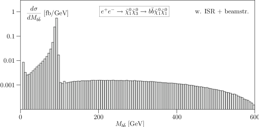
Figure 5: The $b\bar{b}$ invariant mass distribution for the $\tilde{\chi}^{0}_{1}\tilde{\chi}^{0}_{3}$ contribution to $e^{+}e^{-}\to b\bar{b}\tilde{\chi}^{0}_{1}\tilde{\chi}^{0}_{1}$.

An estimate of the effects of the NWA and of Breit-Wigner propagators is shown in Tab. 2. In replacing on-shell intermediate states by Breit-Wigner functions in the SUSY processes (left panel) the total cross section increases by $15\%$. Breaking the cross section down into individual contributions, it becomes apparent that this increase is mainly due to the heavy neutralino channels. In contrast, the $Z$, Higgs and sbottom channels are fairly well-described by the on-shell approximation of Eq. (1). Including the complete set of all tree-level Feynman diagrams with all interferences results in a decrease of $11\%$. Obviously, continuum and interference effects are non-negligible and must be properly taken into account.

Similar considerations apply to the SM background, $e^{+}e^{-}\to b\bar{b}\nu\bar{\nu}$, shown in the right panel of Tab. 2. At a collider energy of $800\;{\rm GeV}$, the SM process is dominated by weak boson fusion, while pair production ($ZZ/ZH$) borders on negligible. For the total cross section, the NWA works well: inserting Breit-Wigner propagators for the intermediate $Z,h$ states increases the rate by a mere $0.6\%$, and including all diagrams with interferences leads to a further increase of only $1.3\%$.

Finally, we compute the effect of ISR and beamstrahlung: the SUSY cross section increases by $15\%$ — a general effect seen for processes dominated by particle pair production well above threshold. (In that range the cross sections are proportional to $1/\hat{s}$ and therefore profit from the reduction in effective energy due to photon radiation.) In contrast, for the SM background, adding ISR and beamstrahlung amounts to a reduction by $8\%$. This is expected for a $t$-channel-dominated process with asymptotically flat energy dependence.

Apart from total cross sections, it is crucial to understand off-shell effects in distributions. They are significant in the neutralino channels $e^{+}e^{-}\to\tilde{\chi}^{0}_{1}\tilde{\chi}_{i}^{0}\;(i=2,3,4)$, the dominant SUSY backgrounds to our sbottom signal. For this mass spectrum, the $\tilde{\chi}^{0}_{2}$ has a three-body decay to $q\bar{q}\tilde{\chi}^{0}_{1}$; here the focus is on $q=b$. The higgsino-like $\tilde{\chi}^{0}_{3}$ has a two-body decay $\tilde{\chi}^{0}_{3}\to Z\tilde{\chi}^{0}_{1}$ with a branching fraction close to $100\%$ [75].

In the complete calculation, neither the decaying $\tilde{\chi}^{0}_{3}$ nor the intermediate $Z$ is forced on-shell. Continuum effects play a role. This explains the differences in the decay spectrum between the full calculation and the approximation using Breit-Wigner propagators, as seen in Fig. 5. There, we include neutralino pair production, $e^{+}e^{-}\to\tilde{\chi}^{0}_{1}\tilde{\chi}^{0}_{3}$. In Fig. 5 we show the $b\bar{b}$ invariant mass spectrum for the process $e^{+}e^{-}\to\tilde{\chi}^{0}_{1}\tilde{\chi}^{0}_{3}\to b\bar{b}\tilde{\chi}^{0}_{1}\tilde{\chi}^{0}_{1}$. Assuming a two-body $\tilde{\chi}^{0}_{3}$ decay, one would expect a sharp Breit-Wigner $Z$ resonance at $91.18\;{\rm GeV}$. Instead, the resonance is not Breit-Wigner-like and is surrounded by a nearly flat continuous distribution at both high and low masses. Clearly, this would not be accounted for by a factorized production–decay approximation. In fact, it stems from a highly off-shell three-body decay $\tilde{\chi}^{0}_{3}\to b\bar{b}\tilde{\chi}^{0}_{1}$ via an intermediate sbottom. As a background to sbottom pair production, this process gives the dominant contribution, because we can easily cut against on-shell neutralino production. The significant low-mass tail explains the $30\%$ enhancement for this channel seen in Tab. 2. Similar reasoning holds for other channels.

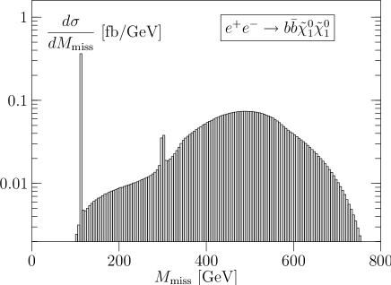
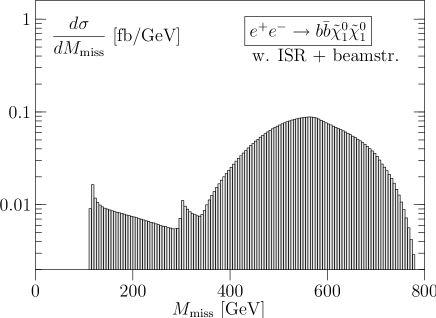
Figure 6: Missing invariant mass spectrum for the full process $e^{+}e^{-}\to b\bar{b}\tilde{\chi}^{0}_{1}\tilde{\chi}^{0}_{1}$: on the left for the partonic process, on the right including ISR and beamstrahlung.

The results in Tab. 2 also demonstrate that photon radiation, both in the elementary process (ISR) and as a semi-classical interaction of the incoming beams (beamstrahlung), cannot be neglected. For the numerical results, ISR is included using the third-order leading-logarithmic approximation [76], and beamstrahlung using the TESLA 800 parameterization in circe [77]. In both cases the photon radiation is predominantly collinear with the incoming beams and therefore invisible. Therefore, all distributions depending on missing momentum, i.e. the momentum of the final-state neutralinos, are distorted by such effects. In the left panel of Fig. 6 we show the missing invariant-mass spectrum for the full process $e^{+}e^{-}\to b\bar{b}\tilde{\chi}^{0}_{1}\tilde{\chi}^{0}_{1}$ without ISR and beamstrahlung. Two narrow peaks are clearly visible, corresponding to the one light and two (unresolved) heavy Higgs bosons. These peaks sit on top of a continuum reaching a maximum around $500\;{\rm GeV}$, dominantly stemming from neutralino and sbottom pairs. We include ISR and beamstrahlung in the right panel of Fig. 6. They tend to wash out the two sharp peaks, with a long tail to higher invariant masses. Without explicitly showing it, we emphasize that the same happens to the SM background, where the $Z$ boson decays invisibly into $\nu\bar{\nu}$.

6.4 Isolating the sbottom-pair signal

According to Tab. 2, the dominant contribution to the $b\bar{b}\tilde{\chi}^{0}_{1}\tilde{\chi}^{0}_{1}$ final state at an ILC is neutralino pair production. To study the sbottom sector, its contribution needs to be isolated with kinematic cuts. In addition, vector boson fusion into $Z$ and Higgs bosons represent non-negligible backgrounds, and have to be reduced accordingly. We see that Higgs boson and heavy sbottom production are of minor importance.

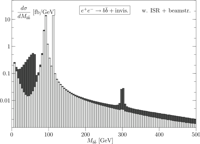
Figure 7: The $b\bar{b}$ invariant mass spectrum for the full process $e^{+}e^{-}\to b\bar{b}$+$E/\hskip 1.99997pt$ with ISR and beamstrahlung. The SM background ($Z\to\nu\bar{\nu}$) with the $Z,h$ peaks is light gray. Dark gray represents all MSSM processes, with two peaks from heavy neutralino and heavy Higgs decays.

An obvious cut for background reduction is on the reconstructed $b\bar{b}$ invariant mass. Fig. 7 shows the distribution for the full process, with all Feynman diagrams and including ISR and beamstrahlung. SM contributions (light gray) and the MSSM (dark) must be superimposed to obtain the complete signal and background result, since neutrinos cannot be distinguished from neutralinos. The spectrum depicted in Fig. 7 has several distinct features: there are narrow peaks at the $h$, $Z$ and $H/A$ boson masses, as well as a broader enhancement around $50\;{\rm GeV}$, associated with the $\tilde{\chi}^{0}_{2}$ three-body decay. (The $\tilde{b}_{1}\tilde{b}_{1}^{*}$ signal does not have any resonance structure and populates the continuum at high invariant $b\bar{b}$ masses.) To remove all resonances we cut away the invariant mass windows:

$$M_{b\bar{b}}<150\;{\rm GeV}\;,\qquad\qquad 250\;{\rm GeV}<M_{b\bar{b}}<350\;{\rm GeV}\;.$$ (7)

This cut retains mostly sbottom-pair signal events, with some continuum background. In the crude NWA (just the simple production channels $\tilde{b}_{1}\tilde{b}_{1}^{*},\tilde{\chi}^{0}_{1}\tilde{\chi}^{0}_{2},\tilde{\chi}^{0}_{1}\tilde{\chi}^{0}_{3}$ and $W^{+}W^{-}\to Z/h$, $ZZ$, $Zh$, $HA$, $\ldots$; times decay matrix elements), these cuts would remove the entire background, while only marginally affecting the signal.

$$\begin{array}[]{|l|rr|}\hline\cr\text{Channel}&\sigma_{\rm BW}~{}[{\rm fb}]&\sigma_{\rm BW}^{\rm cut}~{}[{\rm fb}]\\ \hline\cr Zh&1.335&0.009\\ ZH&0.000&0.000\\ hA&0.000&0.000\\ HA&0.314&0.003\\ \tilde{\chi}^{0}_{1}\tilde{\chi}^{0}_{2}&13.954&0.458\\ \tilde{\chi}^{0}_{1}\tilde{\chi}^{0}_{3}&4.828&0.454\\ \tilde{\chi}^{0}_{1}\tilde{\chi}^{0}_{4}&0.938&0.937\\ \tilde{b}_{1}\tilde{b}_{1}&0.757&0.451\\ \tilde{b}_{1}\tilde{b}_{2}&0.002&0.001\\ \hline\cr\text{Sum}&22.129&2.314\\ \hline\cr\hline\cr\text{Exact}&19.624&0.487\\ \text{w/ISR}&22.552&0.375\\ \hline\cr\end{array}\hskip 56.9055pt\begin{array}[]{|l|rr|}\hline\cr\text{Channel}&\sigma_{\rm BW}~{}[{\rm fb}]&\sigma_{\rm BW}^{\rm cut}~{}[{\rm fb}]\\ \hline\cr Z\bar{\nu}\nu&111.4&2.114\\ h\bar{\nu}\nu&76.4&0.002\\ H\bar{\nu}\nu&0.0&0.000\\ \hline\cr\text{Sum}&187.7&2.117\\ \hline\cr\hline\cr\text{Exact}&190.1&1.765\\ \text{w/ISR}&174.2&1.609\\ \hline\cr\end{array}$$

Table 3: SUSY cross sections contributing to $e^{+}e^{-}\to b\bar{b}\tilde{\chi}^{0}_{1}\tilde{\chi}^{0}_{1}$ (left) and the SM background $e^{+}e^{-}\to b\bar{b}\nu\bar{\nu}$ (right). The left column is the Breit-Wigner approximation without cuts. The right column is after the $M_{b\bar{b}}$ cuts of Eq.(7). We show the results for the incoherent sum of channels, the complete result with all interferences, and the same with ISR and beamstrahlung.

We show the effect of applying this cut in Tab. 3 using the various approximations. In the full calculation we retain $60\%$ of the signal rate. While in the on-shell approximation this cut would remove $100\%$ of the peaked backgrounds, our complete calculation including Breit-Wigner propagators retains a whopping $2.3\,{\rm fb}$ (SUSY) and $2.1\,{\rm fb}$ (SM). Surprisingly, the exact tree-level cross section without ISR is considerably smaller than that: $0.5\,{\rm fb}$ (SUSY, signal+background) and $1.8\,{\rm fb}$ (SM). Obviously, for the background SUSY processes the Breit-Wigner approximation is misleadingly wrong if we force the phase space into the sbottom-signal region. Only the full calculation gives a reliable result.

In the absence of backgrounds, the $b$ jet energy spectrum from sbottom decays exhibits a box-like shape corresponding to the decay kinematics of $\tilde{b}_{1}\to b\tilde{\chi}^{0}_{1}$. Assuming that $m_{\tilde{\chi}^{0}_{1}}$ is known from a threshold scan, the edges of the box would allow a simple kinematical fit to yield a precise determination of $m_{\tilde{b}_{1}}$. The realistic $E_{b}$ distribution appears in Fig. 8. In the left panel we show the $E_{b}$ spectrum for the full process without cuts, including all interferences, and taking ISR and beamstrahlung into account. The large background precludes any identification of a box shape. The right panel displays the same distribution after the $M_{b\bar{b}}$ cuts of Eq.(7) and compares it with the ideal case (no background, no ISR, no cuts) in the same normalization.

The SUSY contribution after cuts (dark area) shows the same kinematical limits as the ideal box, but the edges are washed out by the combined effects of cuts, ISR/beamstrahlung, and continuum background. However, the signal sits atop a sizable leftover SM background. As argued above, this background cannot be realistically simulated by simply concatenating particle production and decays.

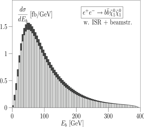
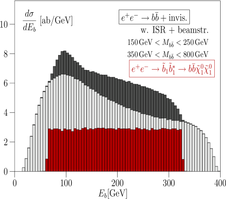
Figure 8: The $E_{b}$ spectrum of the full process $e^{+}e^{-}\to b\bar{b}$+$E/\hskip 1.99997pt$, including all interferences and off-shell effects, plus ISR and beamstrahlung. The light gray histogram is the SM background, dark gray the sum of SUSY processes. The left panel is before the cut of Eq.(7), while the right panel includes the cut. Also in the right panel we show the idealized case (red) of on-shell sbottom production without ISR or beamstrahlung. The SM background is again shown in light gray, while the dark gray shows the sbottom contribution alone.

Without going into detail, we note that for further improvement of the signal-to-background ratio, one could use beam polarization (reducing the $W^{+}W^{-}\to b\bar{b}$ continuum) or a cut on missing invariant mass (to suppress $Z\to\nu\bar{\nu}$). For a final verdict on the measurement of sbottom properties in this decay channel, a realistic analysis must also consider fragmentation, hadronization and detector effects. NLO corrections (at least; if not NNLO) to the signal process must be taken into account to gain some idea about realistic event rates.

7 Summary and Outlook

Phenomenological and experimental (Monte Carlo) analyses for new physics at colliders are usually approached at a level of sophistication which does not match the know-how we have from the Standard Model. For supersymmetric signals at the LHC and an ILC we have carefully studied effects which occur beyond simple $2\to 2$ cross section analyses, using sbottom pair production as a simple example process.

At the LHC, the reconstruction of decay kinematics is the source of essentially all information on heavy new particles. Any observable linked to cross sections instead of kinematical features is bound to suffer from much larger QCD uncertainties. Typical experimental errors from jet energy scaling are of the same order as finite-width effects in the total cross section. However, in relevant distributions, off-shell effects can easily be larger.

QCD off-shell effects also include additional jet radiation from the incoming state. Usually, jet radiation is treated by parton showers in the collinear approximation. For processes with bottom jets in the final state we tested this approximation by computing the effects of two additional bottom jets created through gluon splitting in the initial state. The effects on the rate are typically below $10\%$, and kinematical distributions do indeed change. In our case, distinguishing between initial-state bottom jets and decay bottom jets via rapidity and transverse momentum characteristics does not look promising.

Sbottom pair production at the LHC has the fortunate feature that most of these off-shell effects and combinatorial backgrounds can be removed together with the SM backgrounds, but this feature is by no means guaranteed for general SUSY processes.

At an ILC, the extraction of parameters from kinematic distributions is usually more precise compared to more inclusive measurements. In contrast to the LHC, the typical size $\Gamma/M$ of off-shell effects exceeds the present ILC design experimental precision. It is therefore mandatory for multi-particle final states to include the complete set of off-shell Feynman diagrams in ILC studies, since they can alter signal distributions drastically. This was impressively demonstrated by our study of sbottom pair production where we found up to $400\%$ corrections to production rates from off-shell effects, after standard cuts.

Irreducible SM backgrounds to missing energy signals can strongly distort the shapes of energy and invariant mass distributions. Hence, if we would attempt to extract masses and mass differences from invariant mass distributions at an ILC, we find that we must take into account off-shell effects and additional many-particle intermediate states which can change cross sections dramatically. Simulation of initial state radiation and beamstrahlung is mandatory to describe shapes of resonances and distributions in a realistic linear collider environment.

To compute the effects described above we implemented the MSSM Lagrangian and the proper description of Majorana particles in the matrix element generators madgraph/madevent, o’mega/whizard and amegic++/sherpa. To carefully check these extensions we compared several hundred SUSY production processes numerically, as well as performed a number of unitarity and gauge invariance checks. All results, as well as the SLHA input file, are given in the Appendix — we are confident that this list of processes can serve as a standard reference to generally check MSSM implementations in collider physics or phenomenology tools.

Acknowledgments

All members of this long-term collaboration on the Comparison of Automated Tools for Phenomenological Investigations of SuperSymmetry are grateful to the DESY Theory Group, the Madison Pheno Institute, the Institute for Theoretical Physics at Dresden, and MPI Munich for their continuous support and hospitality. We would also like to thank the Aspen Center for Physics, where much of this work was completed. We would like to thank Gudrun Hiller for her help with the flavor constraints. K. H. is supported in part by Grant-in-Aid for Scientific Research of MEXT, Japan, No. 17540281. T. O., J. R. and W. K. are supported in part by the German Helmholtz-Gemeinschaft, Grant No. VH–NG–005. T. O. is supported in part by Bundesministerium für Bildung und Forschung Germany, Grant No. 05HT1WWA/2. D.R. is supported in part by the U.S. Department of Energy under grant No. DE-FG02-91ER40685. F.K. and S.S. gratefully acknowledge financial support by BMBF.

Appendix A Input Parameters Used in the Comparison

Here we list the input parameters we used, which are in the blocks relevant for our purposes from the SLHA output of the softsusy program:

# SOFTSUSY1.9
# B.C. Allanach, Comput. Phys. Commun. 143 (2002) 305-331, hep-ph/0104145
Block SPINFO         # Program information
     1   SOFTSUSY    # spectrum calculator
     2   1.9         # version number
Block MODSEL  # Select model
     1    1   # sugra
Block SMINPUTS   # Standard Model inputs
#     1    1.27934000e+02   # alpha_em^(-1)(MZ) SM MSbar
     2    1.16639000e-05   # G_Fermi
#     3    1.17200000e-01   # alpha_s(MZ)MSbar
#     4    9.11876000e+01   # MZ(pole)
#     5    4.25000000e+00   # Mb(mb)
#     6    1.74300000e+02   # Mtop(pole)
     7    1.77700000e+00   # Mtau(pole)
Block MINPAR  # SUSY breaking input parameters
     3    1.00000000e+01   # tanb
     4    1.00000000e+00   # sign(mu)
     1    1.00000000e+02   # m0
     2    2.50000000e+02   # m12
     5   -1.00000000e+02   # A0
# Low energy data in SOFTSUSY: MIXING=-1 TOLERANCE=1.00000000e-03
# mgut=2.46245508e+16 GeV
Block MASS   # Mass spectrum
#PDG code      mass              particle
        24     8.04194155e+01   # MW
        25     1.10762900e+02   # h0
        35     4.00615086e+02   # H0
        36     4.00247030e+02   # A0
        37     4.08528577e+02   # H+
   1000001     5.72715810e+02   # ~d_L
   1000002     5.67266777e+02   # ~u_L
   1000003     5.72715810e+02   # ~s_L
   1000004     5.67266777e+02   # ~c_L
   1000005     5.15224253e+02   # ~b_1
   1000006     3.95930570e+02   # ~t_1
   1000011     2.04280587e+02   # ~e_L
   1000012     1.88661921e+02   # ~nue_L
   1000013     2.04280587e+02   # ~mu_L
   1000014     1.88661921e+02   # ~numu_L
   1000015     1.36227332e+02   # ~stau_1
   1000016     1.87777460e+02   # ~nu_tau_L
   1000021     6.07618238e+02   # ~g
   1000022     9.72807171e+01   # ~neutralino(1)
   1000023     1.80959888e+02   # ~neutralino(2)
   1000024     1.80377023e+02   # ~chargino(1)
   1000025    -3.64450624e+02   # ~neutralino(3)
   1000035     3.83149239e+02   # ~neutralino(4)
   1000037     3.83385634e+02   # ~chargino(2)
   2000001     5.46084642e+02   # ~d_R
   2000002     5.47013902e+02   # ~u_R
   2000003     5.46084642e+02   # ~s_R
   2000004     5.47013902e+02   # ~c_R
   2000005     5.43980537e+02   # ~b_2
   2000006     5.85709387e+02   # ~t_2
   2000011     1.45527209e+02   # ~e_R
   2000013     1.45527209e+02   # ~mu_R
   2000015     2.08226705e+02   # ~stau_2
# Higgs mixing
Block alpha   # Effective Higgs mixing parameter
          -1.13731924e-01   # alpha
Block stopmix  # stop mixing matrix
   1  1     5.38076009e-01   # O_{11}
   1  2     8.42896322e-01   # O_{12}
   2  1     8.42896322e-01   # O_{21}
   2  2    -5.38076009e-01   # O_{22}
Block sbotmix  # sbottom mixing matrix
   1  1     9.47748557e-01   # O_{11}
   1  2     3.19018296e-01   # O_{12}
   2  1    -3.19018296e-01   # O_{21}
   2  2     9.47748557e-01   # O_{22}
Block staumix  # stau mixing matrix
  1  1     2.80949722e-01   # O_{11}
  1  2     9.59722488e-01   # O_{12}
  2  1     9.59722488e-01   # O_{21}
  2  2    -2.80949722e-01   # O_{22}
Block nmix  # neutralino mixing matrix
  1  1     9.86069014e-01   # N_{1,1}
  1  2    -5.46217310e-02   # N_{1,2}
  1  3     1.47637908e-01   # N_{1,3}
  1  4    -5.37346696e-02   # N_{1,4}
  2  1     1.02047560e-01   # N_{2,1}
  2  2     9.42730347e-01   # N_{2,2}
  2  3    -2.74969181e-01   # N_{2,3}
  2  4     1.58863895e-01   # N_{2,4}
  3  1    -6.04553550e-02   # N_{3,1}
  3  2     8.97014273e-02   # N_{3,2}
  3  3     6.95501771e-01   # N_{3,3}
  3  4     7.10335196e-01   # N_{3,4}
  4  1    -1.16616232e-01   # N_{4,1}
  4  2     3.16590608e-01   # N_{4,2}
  4  3     6.47203433e-01   # N_{4,3}
  4  4    -6.83592537e-01   # N_{4,4}
Block Umix  # chargino U mixing matrix
  1  1     9.15543496e-01   # U_{1,1}
  1  2    -4.02218978e-01   # U_{1,2}
  2  1     4.02218978e-01   # U_{2,1}
  2  2     9.15543496e-01   # U_{2,2}
Block Vmix  # chargino V mixing matrix
  1  1     9.72352114e-01   # V_{1,1}
  1  2    -2.33519522e-01   # V_{1,2}
  2  1     2.33519522e-01   # V_{2,1}
  2  2     9.72352114e-01   # V_{2,2}
Block hmix Q= 4.64241862e+02  # Higgs mixing parameters
     1     3.58355327e+02   # mu(Q)MSSM DRbar
#     2     9.75144517e+00   # tan beta(Q)MSSM DRbar
     3     2.44921676e+02   # higgs vev(Q)MSSM DRbar
     4     1.69588951e+04   # mA^2(Q)MSSM DRbar
Block au Q= 4.64241862e+02
  1  1     0.00000000e+00   # Au(Q)MSSM DRbar
  2  2     0.00000000e+00   # Ac(Q)MSSM DRbar
  3  3    -5.04528807e+02   # At(Q)MSSM DRbar
Block ad Q= 4.64241862e+02
  1  1     0.00000000e+00   # Ad(Q)MSSM DRbar
  2  2     0.00000000e+00   # As(Q)MSSM DRbar
  3  3    -7.97132778e+02   # Ab(Q)MSSM DRbar
Block ae Q= 4.64241862e+02
  1  1     0.00000000e+00   # Ae(Q)MSSM DRbar
  2  2     0.00000000e+00   # Amu(Q)MSSM DRbar
  3  3    -2.56155534e+02   # Atau(Q)MSSM DRbar

Parameters used with a different value than specified in the above SLHA file are $M_{W}=80.419\,{\rm GeV}$, $M_{Z}=91.188\,{\rm GeV}$. We set all SUSY particle widths to zero, since there are no SUSY particles in the $s$-channel. (The spectrum generator softsusy does not calculate the widths of the SUSY particles. This is instead done by the program sdecay [75].) The only widths used in our comparison are set by hand, $\Gamma_{W}=2.048\,{\rm GeV}$ and $\Gamma_{Z}=2.446\,{\rm GeV}$. All Higgs widths have been set to zero, as well as the electron mass. The third generation quark masses have been given the values $m_{t}=178.0\,{\rm GeV}$ and $m_{b}=4.6\,{\rm GeV}$. For the strong coupling we take $\alpha_{s}(M_{Z})=0.118$. The $G_{F}-M_{Z}-\alpha$ scheme has been used for the SM parameters.

Appendix B Cross Section Values for $2\to 2$ SUSY Processes

The following tables are also maintained at the web page
http://www.sherpa-mc.de/susy_comparison/susy_comparison.html.

B.1 $e^{+}e^{-}$ processes

$\bf{e^{+}e^{-}\to X}$
Final	madgraph/helas		o’mega/whizard		amegic++/sherpa
state	0.5 TeV	2 TeV	0.5 TeV	2 TeV	0.5 TeV	2 TeV
$\tilde{e}_{L}\tilde{e}_{L}^{*}$	54.687(2)	78.864(6)	54.687(3)	78.866(4)	54.6890(7)	78.8670(8)
$\tilde{e}_{R}\tilde{e}_{R}^{*}$	274.69(2)	91.776(8)	274.682(1)	91.776(5)	274.695(3)	91.778(1)
$\tilde{e}_{L}\tilde{e}_{R}^{*}$	75.168(5)	7.237(1)	75.167(3)	7.2372(4)	75.1693(7)	7.23744(7)
$\tilde{\mu}_{L}\tilde{\mu}_{L}^{*}$	22.5471(7)	6.8263(2)	22.5478(9)	6.8265(3)	22.5482(2)	6.82638(7)
$\tilde{\mu}_{R}\tilde{\mu}_{R}^{*}$	51.839(2)	5.8107(2)	51.837(2)	5.8105(2)	51.8401(5)	5.81085(6)
$\tilde{\tau}_{1}\tilde{\tau}_{1}^{*}$	55.582(2)	5.7139(2)	55.580(2)	5.7141(2)	55.5835(6)	5.71399(6)
$\tilde{\tau}_{2}\tilde{\tau}_{2}^{*}$	19.0161(6)	6.5047(2)	19.0174(7)	6.5045(3)	19.0163(2)	6.50473(7)
$\tilde{\tau}_{1}\tilde{\tau}_{2}^{*}$	1.4118(4)	0.21406(1)	1.41191(5)	0.214058(8)	1.41187(1)	0.214067(2)
$\tilde{\nu}_{e}\tilde{\nu}_{e}^{*}$	493.35(2)	272.15(2)	493.38(2)	272.15(1)	493.358(5)	272.155(3)
$\tilde{\nu}_{\mu}\tilde{\nu}_{\mu}^{*}$	14.8632(4)	2.9231(1)	14.8638(6)	2.9232(1)	14.8633(1)	2.92309(3)
$\tilde{\nu}_{\tau}\tilde{\nu}_{\tau}^{*}$	15.1399(5)	2.9246(1)	15.1394(8)	2.9245(1)	15.1403(2)	2.92465(3)
$\tilde{u}_{L}\tilde{u}_{L}^{*}$	—	7.6185(2)	—	7.6188(3)	—	7.61859(8)
$\tilde{u}_{R}\tilde{u}_{R}^{*}$	—	4.6933(1)	—	4.6935(2)	—	4.69342(5)
$\tilde{c}_{L}\tilde{c}_{L}^{*}$	—	7.6185(2)	—	7.6182(3)	—	7.61859(8)
$\tilde{c}_{R}\tilde{c}_{R}^{*}$	—	4.6933(1)	—	4.6933(2)	—	4.69342(5)
$\tilde{t}_{1}\tilde{t}_{1}^{*}$	—	5.9845(4)	—	5.9847(2)	—	5.98459(6)
$\tilde{t}_{2}\tilde{t}_{2}^{*}$	—	5.3794(3)	—	5.3792(2)	—	5.37951(6)
$\tilde{t}_{1}\tilde{t}_{2}^{*}$	—	1.2427(1)	—	1.24264(5)	—	1.24270(1)
$\tilde{d}_{L}\tilde{d}_{L}^{*}$	—	5.2055(1)	—	5.2059(2)	—	5.20563(2)
$\tilde{d}_{R}\tilde{d}_{R}^{*}$	—	1.17588(2)	—	1.17595(5)	—	1.17591(1)
$\tilde{s}_{L}\tilde{s}_{L}^{*}$	—	5.2055(1)	—	5.2058(2)	—	5.20563(2)
$\tilde{s}_{R}\tilde{s}_{R}^{*}$	—	1.17588(2)	—	1.17585(5)	—	1.17591(1)
$\tilde{b}_{1}\tilde{b}_{1}^{*}$	—	4.9388(3)	—	4.9387(2)	—	4.93883(5)
$\tilde{b}_{2}\tilde{b}_{2}^{*}$	—	1.1295(1)	—	1.12946(4)	—	1.12953(1)
$\tilde{b}_{1}\tilde{b}_{2}^{*}$	—	0.51644(3)	—	0.516432(9)	—	0.516447(6)
$\tilde{\chi}^{0}_{1}\tilde{\chi}^{0}_{1}$	240.631(4)	26.3082(2)	240.636(7)	26.3087(9)	240.638(2)	26.3086(3)
$\tilde{\chi}^{0}_{1}\tilde{\chi}^{0}_{2}$	62.377(1)	9.9475(1)	62.374(2)	9.9475(4)	62.3785(6)	9.94778(1)
$\tilde{\chi}^{0}_{1}\tilde{\chi}^{0}_{3}$	7.78117(2)	0.64795(1)	7.78131(4)	0.64796(1)	7.78121(8)	0.647969(6)
$\tilde{\chi}^{0}_{1}\tilde{\chi}^{0}_{4}$	1.03457(3)	1.36561(1)	1.03460(3)	1.36564(5)	1.03460(1)	1.36568(1)
$\tilde{\chi}^{0}_{2}\tilde{\chi}^{0}_{2}$	70.730(2)	18.6841(3)	70.730(3)	18.6845(8)	70.7310(7)	18.6843(2)
$\tilde{\chi}^{0}_{2}\tilde{\chi}^{0}_{3}$	—	1.85588(2)	—	1.85590(4)	—	1.85594(2)
$\tilde{\chi}^{0}_{2}\tilde{\chi}^{0}_{4}$	—	3.03946(4)	—	3.03951(9)	—	3.03949(3)
$\tilde{\chi}^{0}_{3}\tilde{\chi}^{0}_{3}$	—	4.2214(1)e-3	—	4.2214(2)e-3	—	4.22147(4)e-3
$\tilde{\chi}^{0}_{3}\tilde{\chi}^{0}_{4}$	—	9.93621(8)	—	9.9362(3)	—	9.93637(1)
$\tilde{\chi}^{0}_{4}\tilde{\chi}^{0}_{4}$	—	0.135479(1)	—	0.135482(5)	—	0.135479(1)
$\tilde{\chi}_{1}^{+}\tilde{\chi}_{1}^{-}$	162.786(6)	45.079(2)	162.788(7)	45.080(2)	162.786(2)	45.0808(5)
$\tilde{\chi}_{2}^{+}\tilde{\chi}_{2}^{-}$	—	26.9854(3)	—	26.9864(6)	—	26.9857(3)
$\tilde{\chi}_{1}^{+}\tilde{\chi}_{2}^{-}$	—	4.01053(5)	—	4.01053(9)	—	4.01066(4)
$Zh^{0}$	59.377(2)	3.1148(2)	59.376(1)	3.11492(9)	59.3789(6)	3.11491(3)
$ZH^{0}$	6.17904(1)e-4	5.5060(3)e-4	6.179180(5)e-4	5.5058(2)e-4	6.17919(6)e-4	5.50607(6)e-4
$A^{0}h^{0}$	—	5.3434(2)e-4	—	5.3433(2)e-4	—	5.34350(5)e-4
$A^{0}H^{0}$	—	2.37418(7)	—	2.37434(9)	—	2.37422(2)
$H^{+}H^{-}$	—	5.5335(2)	—	5.5339(2)	—	5.53374(6)

B.2 $\tau^{+}\tau^{-}$ processes

$\bf{\tau^{+}\tau^{-}\to X}$
Final	madgraph/helas		o’mega/whizard		amegic++/sherpa
state	0.5 TeV	2 TeV	0.5 TeV	2 TeV	0.5 TeV	2 TeV
$\tilde{\tau}_{1}\tilde{\tau}_{1}^{*}$	257.31(5)	79.63(4)	257.32(1)	79.636(4)	257.30(1)	79.638(4)
$\tilde{\tau}_{2}\tilde{\tau}_{2}^{*}$	46.368(6)	66.86(2)	46.368(2)	66.862(3)	46.372(2)	66.862(3)
$\tilde{\tau}_{1}\tilde{\tau}_{2}^{*}$	81.72(2)	18.96(1)	81.720(3)	18.9588(8)	81.726(4)	18.960(1)
$\tilde{\nu}_{\tau}\tilde{\nu}_{\tau}^{*}$	502.26(7)	272.01(8)	502.27(2)	272.01(1)	502.30(3)	272.01(1)
$\tilde{\chi}^{0}_{1}\tilde{\chi}^{0}_{1}$	249.94(2)	26.431(1)	249.954(9)	26.431(1)	249.96(1)	26.431(1)
$\tilde{\chi}^{0}_{1}\tilde{\chi}^{0}_{2}$	69.967(3)	9.8940(3)	69.969(2)	9.8940(4)	69.968(3)	9.8937(5)
$\tilde{\chi}^{0}_{1}\tilde{\chi}^{0}_{3}$	17.0387(3)	0.7913(1)	17.0394(1)	0.79136(2)	17.040(1)	0.79137(5)
$\tilde{\chi}^{0}_{1}\tilde{\chi}^{0}_{4}$	7.01378(4)	1.50743(3)	7.01414(6)	1.5075(5)	7.0141(4)	1.50740(8)
$\tilde{\chi}^{0}_{2}\tilde{\chi}^{0}_{2}$	82.351(7)	18.887(1)	82.353(3)	18.8879(9)	82.357(4)	18.8896(1)
$\tilde{\chi}^{0}_{2}\tilde{\chi}^{0}_{3}$	—	1.7588(1)	—	1.75884(5)	—	1.7588(1)
$\tilde{\chi}^{0}_{2}\tilde{\chi}^{0}_{4}$	—	2.96384(7)	—	2.9640(1)	—	2.9639(1)
$\tilde{\chi}^{0}_{3}\tilde{\chi}^{0}_{3}$	—	0.046995(4)	—	0.0469966(9)	—	0.046999(2)
$\tilde{\chi}^{0}_{3}\tilde{\chi}^{0}_{4}$	—	8.5852(4)	—	8.5857(3)	—	8.5856(4)
$\tilde{\chi}^{0}_{4}\tilde{\chi}^{0}_{4}$	—	0.26438(2)	—	0.264389(5)	—	0.26437(1)
$\tilde{\chi}_{1}^{+}\tilde{\chi}_{1}^{-}$	185.09(3)	45.15(1)	185.093(6)	45.147(2)	185.10(1)	45.151(2)
$\tilde{\chi}_{2}^{+}\tilde{\chi}_{2}^{-}$	—	26.515(1)	—	26.5162(6)	—	26.515(1)
$\tilde{\chi}_{1}^{+}\tilde{\chi}_{2}^{-}$	—	4.2127(4)	—	4.21267(9)	—	4.2125(2)
$h^{0}h^{0}$	0.3533827(3)	1.242(2)e-4	0.35339(2)	1.2422(3)e-4	0.35340(2)	1.24218(6)e-4
$h^{0}H^{0}$	—	5.167(4)e-3	—	5.1669(3)e-3	—	5.1671(3)e-3
$H^{0}H^{0}$	—	0.07931(3)	—	0.079301(6)	—	0.079311(4)
$A^{0}A^{0}$	—	0.07975(3)	—	0.079758(6)	—	0.079744(4)
$Zh^{0}$	59.591(3)	3.1803(8)	59.589(3)	3.1802(1)	59.602(3)	3.1829(2)
$ZH^{0}$	2.8316(3)	4.671(5)	2.83169(9)	4.6706(3)	2.8318(1)	4.6706(2)
$ZA^{0}$	2.9915(4)	4.682(5)	2.99162(9)	4.6821(3)	2.9917(2)	4.6817(2)
$A^{0}h^{0}$	—	5.143(4)e-3	—	5.1434(3)e-3	—	5.1440(3)e-3
$A^{0}H^{0}$	—	1.4880(2)	—	1.48793(9)	—	1.48802(8)
$H^{+}H^{-}$	—	5.2344(6)	—	5.2344(2)	—	5.2345(3)

B.3 $e^{-}\bar{\nu}_{e}$ processes

$\bf{e^{-}\bar{\nu}_{e}\to X^{-}}$
Final	madgraph/helas		o’mega/whizard		amegic++/sherpa
state	0.5 TeV	2 TeV	0.5 TeV	2 TeV	0.5 TeV	2 TeV
$\tilde{e}_{L}\tilde{\nu}_{e}^{*}$	158.69(1)	67.096(5)	158.694(7)	67.095(3)	158.703(8)	67.100(3)
$\tilde{e}_{R}\tilde{\nu}_{e}^{*}$	68.51(1)	6.547(4)	68.513(3)	6.5470(4)	68.508(3)	6.5469(3)
$\tilde{\mu}_{L}\tilde{\nu}_{\mu}^{*}$	58.492(3)	13.894(1)	58.491(2)	13.8935(5)	58.492(3)	13.8931(7)
$\tilde{\tau}_{1}\tilde{\nu}_{\tau}^{*}$	8.5018(5)	1.1169(1)	8.5021(3)	1.11690(4)	8.5018(4)	1.11696(6)
$\tilde{\tau}_{2}\tilde{\nu}_{\tau}^{*}$	51.792(3)	12.784(1)	51.790(2)	12.7836(5)	51.795(3)	12.7844(6)
$\tilde{\chi}_{1}^{-}\tilde{\chi}^{0}_{1}$	137.414(5)	21.4202(6)	137.416(4)	21.4203(9)	137.426(8)	21.419(2)
$\tilde{\chi}_{1}^{-}\tilde{\chi}^{0}_{2}$	58.797(3)	21.284(2)	58.795(1)	21.283(1)	58.794(3)	21.282(2)
$\tilde{\chi}_{1}^{-}\tilde{\chi}^{0}_{3}$	—	2.2676(1)	—	2.26760(7)	—	2.2678(1)
$\tilde{\chi}_{1}^{-}\tilde{\chi}^{0}_{4}$	—	3.5104(2)	—	3.51046(6)	—	3.5105(2)
$\tilde{\chi}_{2}^{-}\tilde{\chi}^{0}_{1}$	1.16070(5)	1.73602(6)	1.16072(3)	1.73607(6)	1.16066(6)	1.73593(9)
$\tilde{\chi}_{2}^{-}\tilde{\chi}^{0}_{2}$	—	3.6111(3)	—	3.61122(6)	—	3.6113(2)
$\tilde{\chi}_{2}^{-}\tilde{\chi}^{0}_{3}$	—	26.9497(5)	—	26.9511(7)	—	26.952(1)
$\tilde{\chi}_{2}^{-}\tilde{\chi}^{0}_{4}$	—	24.022(1)	—	24.0223(8)	—	24.022(1)

B.4 $\tau^{-}\bar{\nu}_{\tau}$ processes

$\bf{\tau^{-}\bar{\nu}_{\tau}\to X^{-}}$
Final	madgraph/helas		o’mega/whizard		amegic++/sherpa
state	0.5 TeV	2 TeV	0.5 TeV	2 TeV	0.5 TeV	2 TeV
$\tilde{\tau}_{1}\tilde{\nu}_{\tau}^{*}$	84.13(2)	12.272(7)	84.129(3)	12.2724(4)	84.124(4)	12.2719(6)
$\tilde{\tau}_{2}\tilde{\nu}_{\tau}^{*}$	139.86(1)	61.466(7)	139.852(6)	61.463(3)	139.858(7)	61.467(3)
$\tilde{\chi}_{1}^{-}\tilde{\chi}^{0}_{1}$	146.263(6)	21.386(1)	146.265(4)	21.3863(9)	146.27(1)	21.389(2)
$\tilde{\chi}_{1}^{-}\tilde{\chi}^{0}_{2}$	56.218(4)	21.338(3)	56.217(1)	21.336(1)	56.218(5)	21.339(2)
$\tilde{\chi}_{1}^{-}\tilde{\chi}^{0}_{3}$	—	2.2049(1)	—	2.2046(2)	—	2.2050(2)
$\tilde{\chi}_{1}^{-}\tilde{\chi}^{0}_{4}$	—	3.4436(3)	—	3.44365(7)	—	3.4434(3)
$\tilde{\chi}_{2}^{-}\tilde{\chi}^{0}_{1}$	7.5231(2)	1.9569(1)	7.52316(6)	1.95691(6)	7.5234(8)	1.9570(2)
$\tilde{\chi}_{2}^{-}\tilde{\chi}^{0}_{2}$	—	3.4953(3)	—	3.49538(6)	—	3.4955(3)
$\tilde{\chi}_{2}^{-}\tilde{\chi}^{0}_{3}$	—	25.867(1)	—	25.8690(7)	—	25.866(3)
$\tilde{\chi}_{2}^{-}\tilde{\chi}^{0}_{4}$	—	23.199(1)	—	23.1989(8)	—	23.201(2)
$H^{-}h^{0}$	—	0.002422(1)	—	0.0024223(1)	—	0.0024221(1)
$H^{-}H^{0}$	—	4.8560(5)	—	4.8560(3)	—	4.8564(2)
$H^{-}A^{0}$	—	4.8574(5)	—	4.8578(3)	—	4.8576(2)
$W^{-}h^{0}$	133.484(7)	7.537(1)	133.478(5)	7.5376(3)	133.476(7)	7.5377(4)
$W^{-}H^{0}$	57.988(7)	8.543(7)	57.989(2)	8.5432(4)	57.991(3)	8.5435(4)
$W^{-}A^{0}$	58.584(7)	8.567(7)	58.583(2)	8.5672(4)	58.586(3)	8.5679(4)
$ZH^{-}$	17.9854(1)	13.99(1)	17.9860(5)	13.9881(6)	17.986(1)	13.9881(7)

B.5 $b\bar{t}$ processes

$\bf{b\bar{t}\to X^{-}}$
Final	madgraph/helas		o’mega/whizard		amegic++/sherpa
state	0.5 TeV	2 TeV	0.5 TeV	2 TeV	0.5 TeV	2 TeV
$\tilde{b}_{1}\tilde{t}_{1}^{*}$	—	667.4(2)	—	667.45(2)	—	667.53(4)
$\tilde{b}_{1}\tilde{t}_{2}^{*}$	—	609.5(1)	—	609.52(2)	—	609.53(3)
$\tilde{b}_{2}\tilde{t}_{1}^{*}$	—	692.7(1)	—	692.66(2)	—	692.73(4)
$\tilde{b}_{2}\tilde{t}_{2}^{*}$	—	775.7(2)	—	775.71(2)	—	775.69(4)
$\tilde{\chi}_{1}^{-}\tilde{\chi}^{0}_{1}$	37.7535(4)	0.58472(5)	37.75442(7)	0.584741(6)	37.7542(1)	0.58473(2)
$\tilde{\chi}_{1}^{-}\tilde{\chi}^{0}_{2}$	171.662(4)	6.1432(8)	171.6667(6)	6.1435(2)	171.6654(1)	6.1432(3)
$\tilde{\chi}_{1}^{-}\tilde{\chi}^{0}_{3}$	—	7.2061(7)	—	7.20626(9)	—	7.2057(4)
$\tilde{\chi}_{1}^{-}\tilde{\chi}^{0}_{4}$	—	9.7429(7)	—	9.7429(1)	—	9.7428(5)
$\tilde{\chi}_{2}^{-}\tilde{\chi}^{0}_{1}$	17.9155(5)	2.8972(3)	17.91595(4)	2.89723(3)	17.9159(1)	2.8972(1)
$\tilde{\chi}_{2}^{-}\tilde{\chi}^{0}_{2}$	—	8.1076(7)	—	8.10775(8)	—	8.1078(4)
$\tilde{\chi}_{2}^{-}\tilde{\chi}^{0}_{3}$	—	54.043(2)	—	54.046(1)	—	54.050(4)
$\tilde{\chi}_{2}^{-}\tilde{\chi}^{0}_{4}$	—	48.083(1)	—	48.0844(9)	—	48.083(2)
$H^{-}h^{0}$	—	26.660(8)	—	26.660(1)	—	26.666(4)
$H^{-}H^{0}$	—	2.0061(5)	—	2.00611(8)	—	2.0063(2)
$H^{-}A^{0}$	—	1.9083(5)	—	1.90817(8)	—	1.9084(2)
$ZH^{-}$	20.3530(1)	34.76(1)	20.3544(1)	34.766(1)	20.3543(1)	34.764(2)

B.6 $W^{+}W^{-}$ processes

$\bf{W^{+}W^{-}\to X}$
Final	madgraph/helas		o’mega/whizard		amegic++/sherpa
state	0.5 TeV	2 TeV	0.5 TeV	2 TeV	0.5 TeV	2 TeV
$\tilde{e}_{L}\tilde{e}_{L}^{*}$	192.14(2)	26.538(4)	192.145(1)	26.5380(6)	192.151(9)	26.538(1)
$\tilde{e}_{R}\tilde{e}_{R}^{*}$	00014.215(3)	1.0297(3)	00014.2151(4)	1.02966(4)	00014.2153(7)	1.02968(5)
$\tilde{\mu}_{L}\tilde{\mu}_{L}^{*}$	192.14(2)	26.538(4)	192.146(1)	26.5380(6)	192.139(9)	26.540(1)
$\tilde{\mu}_{R}\tilde{\mu}_{R}^{*}$	00014.215(3)	1.0297(3)	00014.2145(4)	1.02972(4)	00014.2153(7)	1.02975(5)
$\tilde{\tau}_{1}\tilde{\tau}_{1}^{*}$	00007.926(2)	0.8328(3)	00007.9266(2)	0.83284(3)	00007.9269(4)	0.83286(4)
$\tilde{\tau}_{2}\tilde{\tau}_{2}^{*}$	168.05(2)	22.419(4)	168.046(1)	22.4195(5)	168.046(8)	22.419(1)
$\tilde{\tau}_{1}\tilde{\tau}_{2}^{*}$	00017.852(3)	2.3294(4)	00017.8521(1)	2.32935(5)	00017.8518(9)	2.3293(1)
$\tilde{\nu}_{e}\tilde{\nu}_{e}^{*}$	157.80(4)	23.487(6)	157.809(3)	23.486(1)	157.803(8)	23.489(1)
$\tilde{\nu}_{\mu}\tilde{\nu}_{\mu}^{*}$	157.80(4)	23.487(6)	157.806(3)	23.487(1)	157.807(8)	23.488(1)
$\tilde{\nu}_{\tau}\tilde{\nu}_{\tau}^{*}$	152.51(4)	23.427(6)	152.509(3)	23.429(1)	152.520(8)	23.429(1)
$\tilde{u}_{L}\tilde{u}_{L}^{*}$	—	41.59(1)	—	41.590(1)	—	41.588(2)
$\tilde{u}_{R}\tilde{u}_{R}^{*}$	—	1.0761(3)	—	1.07608(3)	—	1.07605(5)
$\tilde{c}_{L}\tilde{c}_{L}^{*}$	—	41.59(1)	—	41.588(1)	—	41.599(2)
$\tilde{c}_{R}\tilde{c}_{R}^{*}$	—	1.0761(3)	—	1.07603(3)	—	1.07596(5)
$\tilde{t}_{1}\tilde{t}_{1}^{*}$	—	180.64(1)	—	180.637(4)	—	180.637(9)
$\tilde{t}_{2}\tilde{t}_{2}^{*}$	—	204.46(1)	—	204.461(3)	—	204.47(1)
$\tilde{t}_{1}\tilde{t}_{2}^{*}$	—	85.176(3)	—	85.178(2)	—	85.187(4)
$\tilde{d}_{L}\tilde{d}_{L}^{*}$	—	39.006(7)	—	39.0067(4)	—	39.007(2)
$\tilde{d}_{R}\tilde{d}_{R}^{*}$	—	0.26929(7)	—	0.269305(8)	—	0.26930(1)
$\tilde{s}_{L}\tilde{s}_{L}^{*}$	—	39.006(7)	—	39.0062(4)	—	39.007(2)
$\tilde{s}_{R}\tilde{s}_{R}^{*}$	—	0.26929(7)	—	0.269291(8)	—	0.26930(1)
$\tilde{b}_{1}\tilde{b}_{1}^{*}$	—	141.456(8)	—	141.457(2)	—	141.467(7)
$\tilde{b}_{2}\tilde{b}_{2}^{*}$	—	19.714(1)	—	19.7133(4)	—	19.715(1)
$\tilde{b}_{1}\tilde{b}_{2}^{*}$	—	61.090(4)	—	61.090(1)	—	61.093(3)
$\tilde{\chi}^{0}_{1}\tilde{\chi}^{0}_{1}$	00003.8822(2)	1.2741(4)	00003.8824(1)	1.27423(8)	00003.8821(2)	1.2741(1)
$\tilde{\chi}^{0}_{1}\tilde{\chi}^{0}_{2}$	121.29(1)	24.47(1)	121.2925(7)	24.472(3)	121.296(6)	24.477(1)
$\tilde{\chi}^{0}_{1}\tilde{\chi}^{0}_{3}$	00006.8936(7)	12.880(7)	00006.8934(2)	12.8790(8)	00006.8938(3)	12.8793(6)
$\tilde{\chi}^{0}_{1}\tilde{\chi}^{0}_{4}$	00001.4974(1)	9.707(5)	00001.4973(6)	9.7064(7)	00001.49735(7)	9.7078(4)
$\tilde{\chi}^{0}_{2}\tilde{\chi}^{0}_{2}$	5996.5(4)	1.0415(6)e3	5996.57(2)	1.04150(5)e3	5996.4(3)	1.04148(5)e3
$\tilde{\chi}^{0}_{2}\tilde{\chi}^{0}_{3}$	—	365.6(2)	—	365.615(6)	—	365.63(2)
$\tilde{\chi}^{0}_{2}\tilde{\chi}^{0}_{4}$	—	467.8(2)	—	467.775(8)	—	467.77(2)
$\tilde{\chi}^{0}_{3}\tilde{\chi}^{0}_{3}$	—	82.35(3)	—	82.347(8)	—	82.352(4)
$\tilde{\chi}^{0}_{3}\tilde{\chi}^{0}_{4}$	—	138.20(5)	—	138.18(1)	—	138.205(7)
$\tilde{\chi}^{0}_{4}\tilde{\chi}^{0}_{4}$	—	117.78(4)	—	117.80(1)	—	117.786(6)
$\tilde{\chi}_{1}^{+}\tilde{\chi}_{1}^{-}$	3772(1)	944.3(8)	3771.6(4)	944.2(1)	3771.8(2)	944.32(5)
$\tilde{\chi}_{2}^{+}\tilde{\chi}_{2}^{-}$	—	258.3(2)	—	258.37(4)	—	258.36(1)
$\tilde{\chi}_{1}^{+}\tilde{\chi}_{2}^{-}$	—	131.0(1)	—	130.98(2)	—	130.966(7)
$h^{0}h^{0}$	6023.6(9)	6.057(3)e3	6024.7(4)	6.061(1)e3	6025.0(3)	6.0587(3)e3
$h^{0}H^{0}$	—	2.174(1)	—	2.1752(6)	—	2.1752(1)
$H^{0}H^{0}$	—	6.7515(1)	—	6.7509(11)	—	6.7517(3)
$A^{0}A^{0}$	—	6.7270(1)	—	6.7273(4)	—	6.7274(3)
$Zh^{0}$	75520(13)	8.617(4)e4	75539(7)	8.620(2)e4	75528(4)	8.6181(4)e4
$ZH^{0}$	00001.70948(2)	16.390(8)	00001.70944(8)	16.3939(37)	00001.70971(9)	16.3933(8)
$A^{0}h^{0}$	—	6.0126(3)e-3	—	6.0123(7)e-3	—	6.0130(3)e-3
$A^{0}H^{0}$	—	3.4709(3)	—	3.4708(7)	—	3.4710(2)
$H^{+}H^{-}$	—	19.605(1)	—	19.6060(23)	—	19.605(1)

B.7 $W^{-}Z$ processes

$\bf{W^{-}Z\to X^{-}}$
Final	madgraph/helas		o’mega/whizard		amegic++/sherpa
state	0.5 TeV	2 TeV	0.5 TeV	2 TeV	0.5 TeV	2 TeV
$\tilde{e}_{L}\tilde{\nu}_{e}^{*}$	96.635(6)	15.726(1)	96.639(2)	15.728(2)	96.632(5)	15.7249(8)
$\tilde{\mu}_{L}\tilde{\nu}_{\mu}^{*}$	96.635(6)	15.726(1)	96.638(2)	15.727(2)	96.631(5)	15.7264(8)
$\tilde{\tau}_{1}\tilde{\nu}_{\tau}^{*}$	14.9542(8)	1.427(1)	14.952(1)	1.4268(2)	14.953(1)	1.42747(7)
$\tilde{\tau}_{2}\tilde{\nu}_{\tau}^{*}$	85.875(5)	14.479(1)	85.875(2)	14.478(2)	85.870(4)	14.4780(7)
$\tilde{d}_{L}\tilde{u}_{L}^{*}$	—	24.220(3)	—	24.220(1)	—	24.219(1)
$\tilde{s}_{L}\tilde{c}_{L}^{*}$	—	24.220(3)	—	24.221(1)	—	24.220(1)
$\tilde{b}_{1}\tilde{t}_{1}^{*}$	—	40.676(2)	—	40.676(4)	—	40.677(2)
$\tilde{b}_{2}\tilde{t}_{2}^{*}$	—	8.3717(5)	—	8.3706(7)	—	8.3722(4)
$\tilde{b}_{1}\tilde{t}_{2}^{*}$	—	63.596(3)	—	63.592(6)	—	63.591(3)
$\tilde{b}_{2}\tilde{t}_{1}^{*}$	—	3.9242(2)	—	3.9236(5)	—	3.9244(2)
$\tilde{\chi}^{0}_{1}\tilde{\chi}_{1}^{-}$	61.634(6)	16.389(5)	61.626(3)	16.389(1)	61.633(3)	16.391(1)
$\tilde{\chi}^{0}_{2}\tilde{\chi}_{1}^{-}$	2.8355(7)e3	668.2(4)	2.8350(3)e3	668.1(1)	2.8356(2)e3	668.34(3)
$\tilde{\chi}^{0}_{3}\tilde{\chi}_{1}^{-}$	—	278.5(1)	—	278.53(1)	—	278.58(2)
$\tilde{\chi}^{0}_{4}\tilde{\chi}_{1}^{-}$	—	270.9(1)	—	270.97(2)	—	271.02(2)
$\tilde{\chi}^{0}_{1}\tilde{\chi}_{2}^{-}$	11.7607(3)	12.379(4)	11.7619(7)	12.380(1)	11.7602(6)	12.380(1)
$\tilde{\chi}^{0}_{2}\tilde{\chi}_{2}^{-}$	—	218.3(1)	—	218.38(2)	—	218.40(1)
$\tilde{\chi}^{0}_{3}\tilde{\chi}_{2}^{-}$	—	76.50(3)	—	76.494(5)	—	76.497(4)
$\tilde{\chi}^{0}_{4}\tilde{\chi}_{2}^{-}$	—	97.70(4)	—	97.693(7)	—	97.693(4)
$h^{0}H^{-}$	—	4.439(6)e-3	—	4.4399(5)e-3	—	4.4395(2)e-3
$H^{0}H^{-}$	—	6.1592(6)	—	6.1592(2)	—	6.1589(3)
$A^{0}H^{-}$	—	5.9728(6)	—	5.9726(5)	—	5.9723(3)
$W^{-}h^{0}$	7.620(3)e4	8.29(1)e4	7.6213(6)e4	8.289(2)e4	7.6209(4)e4	8.2909(4)e4
$W^{-}H^{0}$	4.2446(2)	15.78(2)	4.2446(2)	15.783(3)	4.2445(2)	15.7848(8)
$W^{-}A^{0}$	1.07034(3)	0.24799(1)	1.07037(1)	00000.24815(7)	1.07017(6)	0.24801(1)
$ZH^{-}$	0.177241(1)	0.25405(1)	0.17723(2)	0.25403(7)	0.17714(4)	0.25404(1)

B.8 $W^{-}\gamma$ processes

$\bf{W^{-}\gamma\to X^{-}}$
Final	madgraph/helas		o’mega/whizard		amegic++/sherpa
state	0.5 TeV	2 TeV	0.5 TeV	2 TeV	0.5 TeV	2 TeV
$\tilde{e}_{L}\tilde{\nu}_{e}^{*}$	92.93(2)	14.478(3)	92.927(7)	14.477(3)	92.933(5)	14.4789(7)
$\tilde{\mu}_{L}\tilde{\nu}_{\mu}^{*}$	92.93(2)	14.478(3)	92.942(7)	14.479(3)	92.934(5)	14.4782(7)
$\tilde{\tau}_{1}\tilde{\nu}_{\tau}^{*}$	12.098(2)	1.2566(2)	12.100(1)	1.2566(3)	12.1035(6)	1.25669(6)
$\tilde{\tau}_{2}\tilde{\nu}_{\tau}^{*}$	85.17(1)	13.373(2)	85.167(7)	13.372(3)	85.174(4)	13.3731(7)
$\tilde{d}_{L}\tilde{u}_{R}^{*}$	—	6.260(2)	—	6.260(1)	—	6.2605(3)
$\tilde{s}_{L}\tilde{c}_{R}^{*}$	—	6.260(2)	—	6.262(1)	—	6.2605(3)
$\tilde{b}_{1}\tilde{t}_{1}^{*}$	—	5.527(1)	—	5.528(1)	—	5.5279(3)
$\tilde{b}_{2}\tilde{t}_{2}^{*}$	—	0.5418(1)	—	0.5417(1)	—	0.54182(3)
$\tilde{b}_{1}\tilde{t}_{2}^{*}$	—	6.267(1)	—	6.267(1)	—	6.2680(3)
$\tilde{b}_{2}\tilde{t}_{1}^{*}$	—	0.8593(2)	—	0.8595(2)	—	0.85928(4)
$\tilde{\chi}^{0}_{1}\tilde{\chi}_{1}^{-}$	15.824(4)	3.834(2)	15.821(2)	3.8332(6)	15.823(1)	3.8338(2)
$\tilde{\chi}^{0}_{2}\tilde{\chi}_{1}^{-}$	1.2235(2)e3	303.1(1)	1.2235(1)e3	303.04(5)	1.22335(6)e3	303.11(2)
$\tilde{\chi}^{0}_{3}\tilde{\chi}_{1}^{-}$	—	50.91(2)	—	50.902(8)	—	50.909(3)
$\tilde{\chi}^{0}_{4}\tilde{\chi}_{1}^{-}$	—	52.64(2)	—	52.648(8)	—	52.643(3)
$\tilde{\chi}^{0}_{1}\tilde{\chi}_{2}^{-}$	3.0373(3)	6.574(2)	3.03742(7)	00006.5764(9)	3.0373(2)	6.5749(3)
$\tilde{\chi}^{0}_{2}\tilde{\chi}_{2}^{-}$	—	34.00(1)	—	34.003(5)	—	34.000(2)
$\tilde{\chi}^{0}_{3}\tilde{\chi}_{2}^{-}$	—	47.72(1)	—	47.719(7)	—	47.720(2)
$\tilde{\chi}^{0}_{4}\tilde{\chi}_{2}^{-}$	—	59.64(2)	—	59.636(8)	—	59.639(3)
$h^{0}H^{-}$	—	4.519(1)e-3	—	4.5192(8)e-3	—	4.5194(3)e-3
$H^{0}H^{-}$	—	4.961(1)	—	4.9610(9)	—	4.9611(2)
$A^{0}H^{-}$	—	4.966(1)	—	4.9671(9)	—	4.9668(2)
$W^{-}h^{0}$	1.2848(6)e4	1.580(2)e4	1.2855(3)e4	1.5811(4)e4	1.28512(7)e4	1.5801(1)e4
$W^{-}H^{0}$	0.5401(1)	3.016(4)	0.54011(6)	3.0172(7)	0.54016(3)	3.0170(2)

B.9 $ZZ$ processes

$\bf{ZZ\to X}$
Final	madgraph/helas		o’mega/whizard		amegic++/sherpa
state	0.5 TeV	2 TeV	0.5 TeV	2 TeV	0.5 TeV	2 TeV
$\tilde{e}_{L}\tilde{e}_{L}^{*}$	35.791(1)	0003.78984(6)	35.7923(4)	0003.8011(2)	35.792(2)	0003.8009(2)
$\tilde{e}_{R}\tilde{e}_{R}^{*}$	22.9506(3)	0001.92383(3)	22.9508(4)	0001.9234(1)	22.950(1)	0001.9239(1)
$\tilde{\mu}_{L}\tilde{\mu}_{L}^{*}$	35.791(1)	0003.78984(6)	35.7920(4)	0003.8008(2)	35.792(2)	0003.8008(2)
$\tilde{\mu}_{R}\tilde{\mu}_{R}^{*}$	22.9506(3)	0001.92383(3)	22.9509(4)	0001.9239(1)	22.951(1)	0001.9240(2)
$\tilde{\tau}_{1}\tilde{\tau}_{1}^{*}$	19.7282(2)	0001.99982(4)	19.7282(3)	0001.99985(8)	19.729(1)	0001.9998(1)
$\tilde{\tau}_{2}\tilde{\tau}_{2}^{*}$	30.0569(7)	0003.6161(1)	30.0574(2)	0003.6161(1)	30.057(2)	0003.6164(2)
$\tilde{\tau}_{1}\tilde{\tau}_{2}^{*}$	0000.5145(1)	0000.05745(1)	0000.51455(2)	0000.057456(2)	0000.51455(3)	0000.057455(3)
$\tilde{\nu}_{e}\tilde{\nu}_{e}^{*}$	232.51(1)	32.0348(7)	232.517(3)	32.037(2)	232.51(1)	32.035(2)
$\tilde{\nu}_{\mu}\tilde{\nu}_{\mu}^{*}$	232.51(1)	32.0348(7)	232.515(3)	32.037(2)	232.51(1)	32.036(2)
$\tilde{\nu}_{\tau}\tilde{\nu}_{\tau}^{*}$	233.33(1)	32.0709(7)	233.341(3)	32.072(2)	233.34(1)	32.073(2)
$\tilde{u}_{L}\tilde{u}_{L}^{*}$	—	15.6788(4)	—	15.6792(3)	—	15.6799(8)
$\tilde{u}_{R}\tilde{u}_{R}^{*}$	—	0001.20947(1)	—	0001.20948(2)	—	0001.20948(6)
$\tilde{c}_{L}\tilde{c}_{L}^{*}$	—	15.6788(4)	—	15.6791(3)	—	15.6792(8)
$\tilde{c}_{R}\tilde{c}_{R}^{*}$	—	0001.20947(1)	—	0001.20949(2)	—	0001.20950(2)
$\tilde{t}_{1}\tilde{t}_{1}^{*}$	—	262.15(1)	—	262.155(8)	—	262.15(1)
$\tilde{t}_{2}\tilde{t}_{2}^{*}$	—	475.11(2)	—	475.11(1)	—	475.14(2)
$\tilde{t}_{1}\tilde{t}_{2}^{*}$	—	10.7125(2)	—	10.7125(2)	—	10.7128(5)
$\tilde{d}_{L}\tilde{d}_{L}^{*}$	—	30.546(1)	—	30.5474(5)	—	30.547(2)
$\tilde{d}_{R}\tilde{d}_{R}^{*}$	—	0000.238111(1)	—	0000.238127(6)	—	0000.23812(1)
$\tilde{s}_{L}\tilde{s}_{L}^{*}$	—	30.546(1)	—	30.5475(5)	—	30.545(2)
$\tilde{s}_{R}\tilde{s}_{R}^{*}$	—	0000.238111(1)	—	0000.238115(6)	—	0000.23811(1)
$\tilde{b}_{1}\tilde{b}_{1}^{*}$	—	20.7326(7)	—	20.7329(2)	—	20.734(1)
$\tilde{b}_{2}\tilde{b}_{2}^{*}$	—	10.68655(1)	—	10.6865(2)	—	10.6870(5)
$\tilde{b}_{1}\tilde{b}_{2}^{*}$	—	18.6452(1)	—	18.6455(2)	—	18.6454(9)
$h^{0}h^{0}$	7886(1)	7800(5)	7887.5(1)	7802.5(3)	7887.7(4)	7801.3(4)
$h^{0}H^{0}$	—	0002.772(2)	—	0002.7726(2)	—	0002.7727(2)
$H^{0}H^{0}$	—	11.5202(2)	—	11.5209(4)	—	11.5206(6)
$A^{0}A^{0}$	—	11.3523(2)	—	11.3528(4)	—	11.3528(6)
$H^{+}H^{-}$	—	0003.17134(3)	—	0003.17136(5)	—	0003.1714(2)

B.10 $Z\gamma$ processes

$\bf{Z\gamma\to X}$
Final	madgraph/helas		o’mega/whizard		amegic++/sherpa
state	0.5 TeV	2 TeV	0.5 TeV	2 TeV	0.5 TeV	2 TeV
$\tilde{e}_{L}\tilde{e}_{L}^{*}$	64.062(2)	8.7331(2)	64.0633(7)	8.7333(5)	64.062(3)	8.7336(3)
$\tilde{e}_{R}\tilde{e}_{R}^{*}$	50.727(1)	6.0452(1)	50.7284(7)	6.0451(4)	50.728(3)	6.0453(3)
$\tilde{\mu}_{L}\tilde{\mu}_{L}^{*}$	64.062(2)	8.7331(2)	64.0628(7)	8.7327(5)	64.064(3)	8.7329(4)
$\tilde{\mu}_{R}\tilde{\mu}_{R}^{*}$	50.727(1)	6.0452(1)	50.7284(7)	6.0455(4)	50.728(3)	6.0450(3)
$\tilde{\tau}_{1}\tilde{\tau}_{1}^{*}$	36.4564(6)	4.13408(5)	36.4567(6)	4.1336(3)	36.455(2)	4.1339(2)
$\tilde{\tau}_{2}\tilde{\tau}_{2}^{*}$	46.604(1)	6.3910(1)	46.6053(5)	6.3907(4)	46.603(2)	6.3909(3)
$\tilde{\tau}_{1}\tilde{\tau}_{2}^{*}$	24.0433(2)	2.31001(2)	24.0446(3)	2.3102(1)	24.043(1)	2.3100(1)
$\tilde{u}_{L}\tilde{u}_{L}^{*}$	—	10.1947(3)	—	10.1949(2)	—	10.1949(5)
$\tilde{u}_{R}\tilde{u}_{R}^{*}$	—	1.86038(5)	—	1.86042(3)	—	1.8603(1)
$\tilde{c}_{L}\tilde{c}_{L}^{*}$	—	10.1947(3)	—	10.1949(2)	—	10.1950(5)
$\tilde{c}_{R}\tilde{c}_{R}^{*}$	—	1.86038(5)	—	1.86039(3)	—	1.8604(1)
$\tilde{t}_{1}\tilde{t}_{1}^{*}$	—	0.00126511(2)	—	0.00126510(3)	—	0.00126512(6)
$\tilde{t}_{2}\tilde{t}_{2}^{*}$	—	3.44658(6)	—	3.44660(5)	—	3.4465(2)
$\tilde{t}_{1}\tilde{t}_{2}^{*}$	—	19.0977(4)	—	19.0982(7)	—	19.098(1)
$\tilde{d}_{L}\tilde{d}_{L}^{*}$	—	3.70757(7)	—	3.70773(5)	—	3.7077(2)
$\tilde{d}_{R}\tilde{d}_{R}^{*}$	—	0.116431(3)	—	0.116438(2)	—	0.116431(6)
$\tilde{s}_{L}\tilde{s}_{L}^{*}$	—	3.70757(7)	—	3.70774(6)	—	3.7076(2)
$\tilde{s}_{R}\tilde{s}_{R}^{*}$	—	0.116431(3)	—	0.116435(2)	—	0.116431(6)
$\tilde{b}_{1}\tilde{b}_{1}^{*}$	—	3.1278(1)	—	3.12782(6)	—	3.1276(2)
$\tilde{b}_{2}\tilde{b}_{2}^{*}$	—	0.0114499(3)	—	0.0114501(2)	—	0.0114507(6)
$\tilde{b}_{1}\tilde{b}_{2}^{*}$	—	0.53387(1)	—	0.533885(9)	—	0.53388(3)
$H^{+}H^{-}$	—	6.1846(2)	—	6.1849(1)	—	6.1848(3)

B.11 $\gamma\gamma$ processes

$\bf{\gamma\gamma\to X}$
Final	madgraph/helas		o’mega/whizard		amegic++/sherpa
state	0.5 TeV	2 TeV	0.5 TeV	2 TeV	0.5 TeV	2 TeV
$\tilde{e}_{L}\tilde{e}_{L}^{*}$	210.00(1)	29.058(1)	210.005(7)	20.056(5)	210.00(1)	29.060(2)
$\tilde{e}_{R}\tilde{e}_{R}^{*}$	250.32(1)	31.376(1)	250.321(11)	31.381(6)	250.324(12)	31.379(2)
$\tilde{\mu}_{L}\tilde{\mu}_{L}^{*}$	210.00(1)	29.058(1)	209.979(7)	29.041(5)	210.008(12)	29.058(2)
$\tilde{\mu}_{R}\tilde{\mu}_{R}^{*}$	250.32(1)	31.376(1)	250.322(11)	31.379(6)	250.313(13)	31.376(2)
$\tilde{\tau}_{1}\tilde{\tau}_{1}^{*}$	263.35(1)	31.715(1)	263.362(13)	31.714(6)	263.360(13)	31.719(2)
$\tilde{\tau}_{2}\tilde{\tau}_{2}^{*}$	207.62(1)	28.895(1)	207.618(7)	28.897(5)	207.625(10)	28.896(2)
$\tilde{u}_{L}\tilde{u}_{L}^{*}$	—	0009.4531(3)	—	0009.4536(4)	—	0009.4530(4)
$\tilde{u}_{R}\tilde{u}_{R}^{*}$	—	0009.7241(3)	—	0009.7244(5)	—	0009.7236(5)
$\tilde{c}_{L}\tilde{c}_{L}^{*}$	—	0009.4531(3)	—	0009.4534(4)	—	0009.4531(4)
$\tilde{c}_{R}\tilde{c}_{R}^{*}$	—	0009.7241(3)	—	0009.7230(5)	—	0009.7244(5)
$\tilde{t}_{1}\tilde{t}_{1}^{*}$	—	12.5153(5)	—	12.5159(9)	—	12.5157(6)
$\tilde{t}_{2}\tilde{t}_{2}^{*}$	—	0009.2289(3)	—	0009.2298(4)	—	0009.2287(5)
$\tilde{d}_{L}\tilde{d}_{L}^{*}$	—	0000.58654(2)	—	0000.58655(3)	—	0000.58655(3)
$\tilde{d}_{R}\tilde{d}_{R}^{*}$	—	0000.60857(2)	—	0000.60853(3)	—	0000.60857(3)
$\tilde{s}_{L}\tilde{s}_{L}^{*}$	—	0000.58654(2)	—	0000.58656(3)	—	0000.58656(3)
$\tilde{s}_{R}\tilde{s}_{R}^{*}$	—	0000.60857(2)	—	0000.60863(3)	—	0000.60860(3)
$\tilde{b}_{1}\tilde{b}_{1}^{*}$	—	0000.63761(2)	—	0000.63761(3)	—	0000.63759(3)
$\tilde{b}_{2}\tilde{b}_{2}^{*}$	—	0000.61043(2)	—	0000.61045(3)	—	0000.61049(3)
$\tilde{\chi}_{1}^{+}\tilde{\chi}_{1}^{-}$	1458.99(6)	274.0(1)	1459.04(6)	274.020(9)	1458.96(7)	274.01(1)
$\tilde{\chi}_{2}^{+}\tilde{\chi}_{2}^{-}$	—	181.54(3)	—	181.542(6)	—	181.549(9)
$H^{+}H^{-}$	—	20.650(1)	—	20.644(2)	—	20.649(1)

B.12 $g\gamma$ processes

$\bf{g\gamma\to X}$
Final	madgraph/helas		o’mega/whizard		amegic++/sherpa
state	0.5 TeV	2 TeV	0.5 TeV	2 TeV	0.5 TeV	2 TeV
$\tilde{u}_{L}\tilde{u}_{L}^{*}$	—	55.427(1)	—	55.4290(8)	—	55.428(3)
$\tilde{u}_{R}\tilde{u}_{R}^{*}$	—	57.017(1)	—	57.0184(9)	—	57.020(3)
$\tilde{c}_{L}\tilde{c}_{L}^{*}$	—	55.427(1)	—	55.4288(8)	—	55.430(3)
$\tilde{c}_{R}\tilde{c}_{R}^{*}$	—	57.017(1)	—	57.0175(9)	—	57.019(3)
$\tilde{t}_{1}\tilde{t}_{1}^{*}$	—	73.382(2)	—	73.382(2)	—	73.383(4)
$\tilde{t}_{2}\tilde{t}_{2}^{*}$	—	54.113(1)	—	54.1136(8)	—	54.113(3)
$\tilde{d}_{L}\tilde{d}_{L}^{*}$	—	13.7565(4)	—	13.7569(2)	—	13.7560(7)
$\tilde{d}_{R}\tilde{d}_{R}^{*}$	—	14.2733(4)	—	14.2737(2)	—	14.2740(7)
$\tilde{s}_{L}\tilde{s}_{L}^{*}$	—	13.7565(4)	—	13.7568(2)	—	13.7575(7)
$\tilde{s}_{R}\tilde{s}_{R}^{*}$	—	14.2733(4)	—	14.2735(2)	—	14.2731(7)
$\tilde{b}_{1}\tilde{b}_{1}^{*}$	—	14.9542(4)	—	14.9546(3)	—	14.9540(7)
$\tilde{b}_{2}\tilde{b}_{2}^{*}$	—	14.3169(4)	—	14.3171(2)	—	14.3183(7)

B.13 $gZ$ processes

$\bf{gZ\to X}$
Final	madgraph/helas		o’mega/whizard		amegic++/sherpa
state	0.5 TeV	2 TeV	0.5 TeV	2 TeV	0.5 TeV	2 TeV
$\tilde{u}_{L}\tilde{u}_{L}^{*}$	—	59.776(2)	—	59.7774(9)	—	59.778(3)
$\tilde{u}_{R}\tilde{u}_{R}^{*}$	—	10.9082(3)	—	10.9085(2)	—	10.9079(5)
$\tilde{c}_{L}\tilde{c}_{L}^{*}$	—	59.776(2)	—	59.7772(9)	—	59.778(3)
$\tilde{c}_{R}\tilde{c}_{R}^{*}$	—	10.9082(3)	—	10.9084(2)	—	10.9088(5)
$\tilde{t}_{1}\tilde{t}_{1}^{*}$	—	0.0074179(2)	—	0.0074179(2)	—	0.0074182(4)
$\tilde{t}_{2}\tilde{t}_{2}^{*}$	—	20.2088(5)	—	20.2091(3)	—	20.208(1)
$\tilde{t}_{1}\tilde{t}_{2}^{*}$	—	111.978(3)	—	111.986(4)	—	111.980(6)
$\tilde{d}_{L}\tilde{d}_{L}^{*}$	—	86.956(2)	—	86.9615(1)	—	86.960(4)
$\tilde{d}_{R}\tilde{d}_{R}^{*}$	—	2.73075(7)	—	2.73090(4)	—	2.7308(1)
$\tilde{s}_{L}\tilde{s}_{L}^{*}$	—	86.956(2)	—	86.959(1)	—	86.956(4)
$\tilde{s}_{R}\tilde{s}_{R}^{*}$	—	2.73075(7)	—	2.73078(4)	—	2.7308(1)
$\tilde{b}_{1}\tilde{b}_{1}^{*}$	—	73.359(2)	—	73.360(1)	—	73.354(4)
$\tilde{b}_{2}\tilde{b}_{2}^{*}$	—	0.268544(7)	—	0.268554(4)	—	0.26857(1)
$\tilde{b}_{1}\tilde{b}_{2}^{*}$	—	12.5213(3)	—	12.5214(2)	—	12.5214(6)

B.14 $gW^{-}$ processes

$\bf{gW^{-}\to X^{-}}$
Final	madgraph/helas		o’mega/whizard		amegic++/sherpa
state	0.5 TeV	2 TeV	0.5 TeV	2 TeV	0.5 TeV	2 TeV
$\tilde{d}_{L}\tilde{u}_{L}^{*}$	—	187.611(5)	—	187.616(3)	—	187.604(8)
$\tilde{s}_{R}\tilde{c}_{R}^{*}$	—	187.611(5)	—	187.617(3)	—	187.619(8)
$\tilde{b}_{1}\tilde{t}_{1}^{*}$	—	138.625(2)	—	138.625(4)	—	138.624(7)
$\tilde{b}_{2}\tilde{t}_{2}^{*}$	—	16.5094(3)	—	16.5095(3)	—	16.5088(8)
$\tilde{b}_{1}\tilde{t}_{2}^{*}$	—	195.686(1)	—	195.692(4)	—	195.701(9)
$\tilde{b}_{2}\tilde{t}_{1}^{*}$	—	20.7535(5)	—	20.7532(7)	—	20.753(1)

B.15 $gg$ processes

$\bf{gg\to X}$
Final	madgraph/helas		o’mega/whizard		amegic++/sherpa
state	0.5 TeV	2 TeV	0.5 TeV	2 TeV	0.5 TeV	2 TeV
$\tilde{g}\tilde{g}$	—	13575(2)	—	13575.6(1)	—	13575.8(7)
$\tilde{u}_{L}\tilde{u}_{L}^{*}$	—	000185.60(2)	—	000185.615(3)	—	000185.61(1)
$\tilde{u}_{R}\tilde{u}_{R}^{*}$	—	000191.58(2)	—	000191.590(3)	—	000191.59(1)
$\tilde{c}_{L}\tilde{c}_{L}^{*}$	—	000185.60(2)	—	000185.612(3)	—	000185.61(1)
$\tilde{c}_{R}\tilde{c}_{R}^{*}$	—	000191.58(2)	—	000191.588(3)	—	000191.59(1)
$\tilde{t}_{1}\tilde{t}_{1}^{*}$	—	000250.70(2)	—	000250.71(1)	—	000250.70(1)
$\tilde{t}_{2}\tilde{t}_{2}^{*}$	—	000180.54(2)	—	000180.541(3)	—	000180.54(1)
$\tilde{d}_{L}\tilde{d}_{L}^{*}$	—	000184.07(2)	—	000184.081(3)	—	000184.09(1)
$\tilde{d}_{R}\tilde{d}_{R}^{*}$	—	000191.87(2)	—	000191.875(3)	—	000191.87(1)
$\tilde{s}_{L}\tilde{s}_{L}^{*}$	—	000184.07(2)	—	000184.079(3)	—	000184.08(1)
$\tilde{s}_{R}\tilde{s}_{R}^{*}$	—	000191.87(2)	—	000191.873(3)	—	000191.86(1)
$\tilde{b}_{1}\tilde{b}_{1}^{*}$	—	000201.88(2)	—	000201.884(4)	—	000201.90(1)
$\tilde{b}_{2}\tilde{b}_{2}^{*}$	—	000192.52(2)	—	000192.516(3)	—	000192.53(1)

B.16 $u\bar{u}$ processes

$\bf{u\bar{u}\to X}$
Final	madgraph/helas		o’mega/whizard		amegic++/sherpa
state	0.5 TeV	2 TeV	0.5 TeV	2 TeV	0.5 TeV	2 TeV
$\tilde{g}\tilde{g}$	—	1.1377(2)e3	—	1.1378(2)e3	—	1.1377(1)e3
$\tilde{e}_{L}\tilde{e}_{L}^{*}$	0005.169(1)	1.5467(3)	0005.1698(9)	1.5469(2)	0005.1700(3)	1.54698(8)
$\tilde{e}_{R}\tilde{e}_{R}^{*}$	0006.538(1)	0.7318(1)	0006.538(1)	0.7318(1)	0006.5379(3)	0.73179(4)
$\tilde{\mu}_{L}\tilde{\mu}_{L}^{*}$	0005.169(1)	1.5467(3)	0005.1687(9)	1.5466(3)	0005.1693(3)	1.54679(8)
$\tilde{\mu}_{R}\tilde{\mu}_{R}^{*}$	0006.538(1)	0.7318(1)	0006.536(1)	0.7316(1)	0006.5387(3)	0.73189(4)
$\tilde{\tau}_{1}\tilde{\tau}_{1}^{*}$	0006.993(1)	0.7195(1)	0006.992(1)	0.7194(1)	0006.9935(3)	0.71949(4)
$\tilde{\tau}_{2}\tilde{\tau}_{2}^{*}$	0004.1263(7)	1.3962(2)	0004.1246(7)	1.3957(2)	0004.1269(2)	1.39617(7)
$\tilde{\tau}_{1}\tilde{\tau}_{2}^{*}$	0000.5420(1)	0.08218(1)	0000.54193(9)	0.08217(1)	0000.54199(3)	0.082184(4)
$\tilde{\nu}_{e}\tilde{\nu}_{e}^{*}$	0005.7063(5)	1.1222(2)	0005.706(1)	1.1222(2)	0005.7064(3)	1.12224(6)
$\tilde{\nu}_{\mu}\tilde{\nu}_{\mu}^{*}$	0005.7063(5)	1.1222(2)	0005.704(1)	1.1217(2)	0005.7070(3)	1.12237(6)
$\tilde{\nu}_{\tau}\tilde{\nu}_{\tau}^{*}$	0005.812(1)	1.1228(2)	0005.813(1)	1.1229(2)	0005.8126(3)	1.12282(6)
$\tilde{u}_{L}\tilde{u}_{L}^{*}$	—	799.6(1)	—	799.6(1)	—	799.63(4)
$\tilde{u}_{R}\tilde{u}_{R}^{*}$	—	879.7(1)	—	879.7(1)	—	879.75(4)
$\tilde{u}_{L}\tilde{u}_{R}^{*}$	—	784.1(2)	—	784.16(3)	—	784.15(4)
$\tilde{c}_{L}\tilde{c}_{L}^{*}$	—	178.39(1)	—	178.39(2)	—	178.398(9)
$\tilde{c}_{R}\tilde{c}_{R}^{*}$	—	185.63(2)	—	185.62(2)	—	185.655(9)
$\tilde{t}_{1}\tilde{t}_{1}^{*}$	—	245.12(2)	—	245.11(3)	—	245.10(1)
$\tilde{t}_{2}\tilde{t}_{2}^{*}$	—	169.22(1)	—	169.22(2)	—	169.223(8)
$\tilde{t}_{1}\tilde{t}_{2}^{*}$	—	0.47708(4)	—	0.47714(8)	—	0.47712(2)
$\tilde{d}_{L}\tilde{d}_{L}^{*}$	—	166.63(2)	—	166.60(2)	—	166.621(8)
$\tilde{d}_{R}\tilde{d}_{R}^{*}$	—	185.58(2)	—	185.56(3)	—	185.60(1)
$\tilde{s}_{L}\tilde{s}_{L}^{*}$	—	175.69(1)	—	175.68(2)	—	175.686(9)
$\tilde{s}_{R}\tilde{s}_{R}^{*}$	—	185.58(2)	—	185.58(2)	—	185.578(9)
$\tilde{b}_{1}\tilde{b}_{1}^{*}$	—	200.37(2)	—	200.364(8)	—	200.38(1)
$\tilde{b}_{2}\tilde{b}_{2}^{*}$	—	186.50(2)	—	186.500(7)	—	186.51(1)
$\tilde{b}_{1}\tilde{b}_{2}^{*}$	—	0.19827(2)	—	0.198272(8)	—	0.19827(1)
$\tilde{\chi}^{0}_{1}\tilde{\chi}^{0}_{1}$	0002.2483(1)	1.2164(1)	0002.24829(2)	1.2165(1)	0002.2483(1)	1.2165(2)
$\tilde{\chi}^{0}_{1}\tilde{\chi}^{0}_{2}$	0000.053855(3)	0.10850(1)	0000.0538560(9)	0.10850(1)	0000.053855(3)	0.108493(5)
$\tilde{\chi}^{0}_{1}\tilde{\chi}^{0}_{3}$	0000.524518(4)	0.096758(1)	0000.524526(3)	0.096752(5)	0000.52450(3)	0.096763(5)
$\tilde{\chi}^{0}_{1}\tilde{\chi}^{0}_{4}$	0009.8233(3)e-3	0.067303(3)	0009.82339(8)e-3	0.067293(6)	0009.8238(5)e-3	0.067308(3)
$\tilde{\chi}^{0}_{2}\tilde{\chi}^{0}_{2}$	0003.66463(5)	4.2298(3)	0003.66472(3)	4.2296(4)	0003.6646(2)	4.2298(3)
$\tilde{\chi}^{0}_{2}\tilde{\chi}^{0}_{3}$	—	0.21148(3)	—	0.211458(8)	—	0.21147(1)
$\tilde{\chi}^{0}_{2}\tilde{\chi}^{0}_{4}$	—	0.55025(5)	—	0.55025(8)	—	0.55028(3)
$\tilde{\chi}^{0}_{3}\tilde{\chi}^{0}_{3}$	—	3.3843(1)e-4	—	3.3843(1)e-4	—	3.3844(2)e-4
$\tilde{\chi}^{0}_{3}\tilde{\chi}^{0}_{4}$	—	4.4435(3)	—	4.4433(2)	—	4.4436(2)
$\tilde{\chi}^{0}_{4}\tilde{\chi}^{0}_{4}$	—	0.016385(3)	—	0.016389(3)	—	0.016386(1)
$\tilde{\chi}_{1}^{+}\tilde{\chi}_{1}^{-}$	153.97(2)	10.732(5)	153.977(2)	10.734(2)	153.964(8)	10.7329(5)
$\tilde{\chi}_{2}^{+}\tilde{\chi}_{2}^{-}$	—	5.0402(5)	—	5.0401(2)	—	5.0400(3)
$\tilde{\chi}_{1}^{+}\tilde{\chi}_{2}^{-}$	—	1.5363(2)	—	1.5362(2)	—	1.5363(1)
$Zh^{0}$	22.795(2)	1.1958(1)	22.797(2)	1.1960(2)	22.798(1)	1.19582(6)
$ZH^{0}$	0002.37220(1)e-4	2.1138(2)e-4	0002.37224(1)e-4	2.1142(4)e-4	0002.3723(1)e-4	2.1141(1)e-4

B.17 $d\bar{d}$ processes

$\bf{d\bar{d}\to X}$
Final	madgraph/helas		o’mega/whizard		amegic++/sherpa
state	0.5 TeV	2 TeV	0.5 TeV	2 TeV	0.5 TeV	2 TeV
$\tilde{g}\tilde{g}$	—	1.1333(2)e3	—	1.1334(2)e3	—	1.13338(5)e3
$\tilde{e}_{L}\tilde{e}_{L}^{*}$	3.3467(6)	0.9844(2)	3.3472(6)	0.9845(2)	3.3473(2)	0.98453(5)
$\tilde{e}_{R}\tilde{e}_{R}^{*}$	2.0046(3)	0.21577(4)	2.0047(3)	0.21578(4)	2.0047(1)	0.21577(1)
$\tilde{\mu}_{L}\tilde{\mu}_{L}^{*}$	3.3467(6)	0.9844(2)	3.3465(6)	0.9843(2)	3.3469(2)	0.98435(5)
$\tilde{\mu}_{R}\tilde{\mu}_{R}^{*}$	2.0046(3)	0.21577(4)	2.0041(3)	0.21572(4)	2.0049(1)	0.21578(1)
$\tilde{\tau}_{1}\tilde{\tau}_{1}^{*}$	1.7274(3)	0.17266(3)	1.7271(3)	0.17264(3)	1.7273(1)	0.17265(1)
$\tilde{\tau}_{2}\tilde{\tau}_{2}^{*}$	2.4580(4)	0.8175(1)	2.4570(4)	0.8171(1)	2.4582(1)	0.81753(4)
$\tilde{\tau}_{1}\tilde{\tau}_{2}^{*}$	0.6951(1)	0.10539(2)	0.6950(1)	0.10538(2)	0.69505(4)	0.105383(5)
$\tilde{\nu}_{e}\tilde{\nu}_{e}^{*}$	7.3174(1)	1.4391(2)	7.318(1)	1.4391(2)	7.3177(4)	1.43913(7)
$\tilde{\nu}_{\mu}\tilde{\nu}_{\mu}^{*}$	7.3174(1)	1.4391(2)	7.314(1)	1.4385(3)	7.3186(4)	1.43930(7)
$\tilde{\nu}_{\tau}\tilde{\nu}_{\tau}^{*}$	7.454(1)	1.4398(2)	7.454(1)	1.4400(2)	7.4539(4)	1.43987(7)
$\tilde{u}_{L}\tilde{u}_{L}^{*}$	—	174.67(4)	—	174.67(2)	—	174.678(9)
$\tilde{u}_{R}\tilde{u}_{R}^{*}$	—	185.21(2)	—	185.19(3)	—	185.228(9)
$\tilde{c}_{L}\tilde{c}_{L}^{*}$	—	178.11(1)	—	178.10(2)	—	178.113(9)
$\tilde{c}_{R}\tilde{c}_{R}^{*}$	—	185.21(2)	—	185.21(2)	—	185.212(9)
$\tilde{t}_{1}\tilde{t}_{1}^{*}$	—	244.45(2)	—	244.45(3)	—	244.44(1)
$\tilde{t}_{2}\tilde{t}_{2}^{*}$	—	168.81(1)	—	168.80(2)	—	168.812(8)
$\tilde{t}_{1}\tilde{t}_{2}^{*}$	—	0.61179(5)	—	0.61183(8)	—	0.61184(3)
$\tilde{d}_{L}\tilde{d}_{L}^{*}$	—	790.4(1)	—	790.3(1)	—	790.38(4)
$\tilde{d}_{R}\tilde{d}_{R}^{*}$	—	927.1(1)	—	926.9(1)	—	927.11(5)
$\tilde{s}_{L}\tilde{s}_{L}^{*}$	—	175.92(1)	—	175.92(2)	—	175.920(9)
$\tilde{s}_{R}\tilde{s}_{R}^{*}$	—	185.48(2)	—	185.47(2)	—	185.474(9)
$\tilde{b}_{1}\tilde{b}_{1}^{*}$	—	200.54(2)	—	200.54(3)	—	200.57(1)
$\tilde{b}_{2}\tilde{b}_{2}^{*}$	—	186.38(2)	—	186.37(2)	—	186.384(9)
$\tilde{b}_{1}\tilde{b}_{2}^{*}$	—	0.25425(2)	—	0.25429(5)	—	0.25426(1)
$\tilde{\chi}^{0}_{1}\tilde{\chi}^{0}_{1}$	0.118931(1)	0.079120(5)	0.1189331(7)	0.079125(4)	0.118938(5)	0.079118(5)
$\tilde{\chi}^{0}_{1}\tilde{\chi}^{0}_{2}$	0.249928(5)	0.34310(3)	0.249935(1)	0.34310(2)	0.24992(1)	0.34309(2)
$\tilde{\chi}^{0}_{1}\tilde{\chi}^{0}_{3}$	0.81721(1)	0.17387(1)	0.817225(4)	0.173875(3)	0.81722(5)	0.17387(1)
$\tilde{\chi}^{0}_{1}\tilde{\chi}^{0}_{4}$	0.0212680(5)	0.140018(3)	0.0212673(2)	0.140020(3)	0.021268(1)	0.14003(1)
$\tilde{\chi}^{0}_{2}\tilde{\chi}^{0}_{2}$	1.93986(1)	3.1013(3)	1.939907(9)	3.1011(2)	1.9399(1)	3.1012(2)
$\tilde{\chi}^{0}_{2}\tilde{\chi}^{0}_{3}$	—	1.07903(5)	—	1.07909(2)	—	1.07910(5)
$\tilde{\chi}^{0}_{2}\tilde{\chi}^{0}_{4}$	—	1.1685(1)	—	1.16852(6)	—	1.16868(5)
$\tilde{\chi}^{0}_{3}\tilde{\chi}^{0}_{3}$	—	2.66293(3)e-3	—	2.66298(4)e-3	—	2.6631(1)e-3
$\tilde{\chi}^{0}_{3}\tilde{\chi}^{0}_{4}$	—	4.7678(5)	—	4.76810(9)	—	4.7678(3)
$\tilde{\chi}^{0}_{4}\tilde{\chi}^{0}_{4}$	—	0.08799(1)	—	0.087994(6)	—	0.087993(5)
$\tilde{\chi}_{1}^{+}\tilde{\chi}_{1}^{-}$	137.16(2)	10.508(5)	137.161(3)	10.504(2)	137.17(1)	10.5073(5)
$\tilde{\chi}_{2}^{+}\tilde{\chi}_{2}^{-}$	—	4.4960(5)	—	4.4954(1)	—	4.49605(5)
$\tilde{\chi}_{1}^{+}\tilde{\chi}_{2}^{-}$	—	0.7742(2)	—	0.77407(5)	—	0.77420(5)
$Zh^{0}$	29.232(2)	1.5335(2)	29.235(3)	1.5337(3)	29.235(1)	1.53363(8)
$ZH^{0}$	3.04205(1)e-4	2.7107(3)e-4	3.0421(2)e-4	2.7112(5)e-4	3.0421(1)e-4	2.7109(1)e-4

B.18 $b\bar{b}$ processes

$\bf{b\bar{b}\to X}$
Final	madgraph/helas		o’mega/whizard		amegic++/sherpa
state	0.5 TeV	2 TeV	0.5 TeV	2 TeV	0.5 TeV	2 TeV
$\tilde{b}_{1}\tilde{b}_{1}^{*}$	—	896.9(1)	—	896.92(3)	—	896.96(4)
$\tilde{b}_{2}\tilde{b}_{2}^{*}$	—	933.1(1)	—	933.08(3)	—	933.09(5)
$\tilde{b}_{1}\tilde{b}_{2}^{*}$	—	742.4(1)	—	742.46(2)	—	742.48(4)
$\tilde{t}_{1}\tilde{t}_{1}^{*}$	—	475.0(1)	—	475.02(2)	—	475.05(3)
$\tilde{t}_{2}\tilde{t}_{2}^{*}$	—	178.05(2)	—	178.057(7)	—	178.072(9)
$\tilde{t}_{1}\tilde{t}_{2}^{*}$	—	50.580(6)	—	50.581(2)	—	50.583(2)
$\tilde{\chi}^{0}_{1}\tilde{\chi}^{0}_{1}$	6.07876(2)	0.096781(3)	6.078898(4)	0.096786(2)	6.0788(3)	0.096782(4)
$\tilde{\chi}^{0}_{1}\tilde{\chi}^{0}_{2}$	27.5227(1)	0.44563(1)	27.52342(2)	0.445637(9)	27.523(1)	0.44564(2)
$\tilde{\chi}^{0}_{1}\tilde{\chi}^{0}_{3}$	11.19120(1)	0.13673(1)	11.191450(4)	0.1367346(7)	11.1909(6)	0.136730(7)
$\tilde{\chi}^{0}_{1}\tilde{\chi}^{0}_{4}$	4.487214(3)	0.106440(6)	4.487316(1)	0.1064429(7)	4.4876(2)	0.106455(6)
$\tilde{\chi}^{0}_{2}\tilde{\chi}^{0}_{2}$	31.52534(5)	3.5455(1)	31.52604(1)	3.54561(9)	31.525(1)	3.5458(2)
$\tilde{\chi}^{0}_{2}\tilde{\chi}^{0}_{3}$	—	0.92863(6)	—	0.928660(6)	—	0.92869(5)
$\tilde{\chi}^{0}_{2}\tilde{\chi}^{0}_{4}$	—	1.08817(1)	—	1.08823(1)	—	1.08829(6)
$\tilde{\chi}^{0}_{3}\tilde{\chi}^{0}_{3}$	—	0.26420(1)	—	0.264224(9)	—	0.26421(1)
$\tilde{\chi}^{0}_{3}\tilde{\chi}^{0}_{4}$	—	2.7853(2)	—	2.78541(3)	—	2.7856(1)
$\tilde{\chi}^{0}_{4}\tilde{\chi}^{0}_{4}$	—	0.46431(1)	—	0.46432(1)	—	0.46431(2)
$\tilde{\chi}_{1}^{+}\tilde{\chi}_{1}^{-}$	162.814(8)	13.912(2)	162.816(5)	13.9123(6)	162.802(8)	13.9123(7)
$\tilde{\chi}_{2}^{+}\tilde{\chi}_{2}^{-}$	—	104.770(3)	—	104.774(2)	—	104.784(5)
$\tilde{\chi}_{1}^{+}\tilde{\chi}_{2}^{-}$	—	6.7892(3)	—	6.78942(9)	—	6.7892(3)
$h^{0}h^{0}$	0.797127(4)	7.62(2)e-4	0.79711(4)	7.6246(1)e-4	0.79715(4)	7.6252(4)e-4
$h^{0}H^{0}$	—	0.06106(6)	—	0.061079(3)	—	0.061084(3)
$H^{0}H^{0}$	—	1.1850(5)	—	1.18500(9)	—	1.18503(6)
$A^{0}A^{0}$	—	1.1935(5)	—	1.19373(9)	—	1.19368(6)
$A^{0}h^{0}$	—	0.07681(6)	—	0.076825(4)	—	0.076823(4)
$A^{0}H^{0}$	—	2.406(1)	—	2.4064(1)	—	2.4066(1)
$Zh^{0}$	30.490(1)	1.782(1)	30.487(1)	1.78212(5)	30.492(2)	1.78209(9)
$ZH^{0}$	50.837(1)	16.98(2)	50.838(1)	16.9839(8)	50.840(3)	16.9849(8)
$ZA^{0}$	52.024(1)	17.01(2)	52.025(1)	17.0182(8)	52.023(3)	17.0163(9)
$H^{+}H^{-}$	—	2.3187(6)	—	2.31882(9)	—	2.3188(1)

B.19 $qg$ processes

$\bf{qg\to X}$
Process	madgraph/helas		o’mega/whizard		amegic++/sherpa
	0.5 TeV	2 TeV	0.5 TeV	2 TeV	0.5 TeV	2 TeV
$ug\to\tilde{u}_{L}\tilde{g}$	—	3405.0(5)	—	3405.2(3)	—	3404.8(2)
$ug\to\tilde{u}_{R}\tilde{g}$	—	3460.0(5)	—	3460.0(3)	—	3460.4(2)
$dg\to\tilde{d}_{L}\tilde{g}$	—	3390.0(5)	—	3390.5(3)	—	3390.0(2)
$dg\to\tilde{d}_{R}\tilde{g}$	—	3462.5(5)	—	3462.5(3)	—	3462.0(2)

B.20 Two identical fermions as initial state

$\bf{ff\to X}$
Process	madgraph/helas		o’mega/whizard		amegic++/sherpa
	0.5 TeV	2 TeV	0.5 TeV	2 TeV	0.5 TeV	2 TeV
$e^{-}e^{-}\to\tilde{e}_{L}\tilde{e}_{L}$	520.30(4)	36.83(3)	520.31(3)	36.836(2)	520.32(3)	36.832(2)
$e^{-}e^{-}\to\tilde{e}_{R}\tilde{e}_{R}$	459.6(1)	28.65(3)	459.59(1)	28.650(3)	459.63(3)	28.651(2)
$e^{-}e^{-}\to\tilde{e}_{L}\tilde{e}_{R}$	160.04(1)	56.55(2)	159.96(2)	56.522(8)	160.04(2)	56.545(3)
$uu\to\tilde{u}_{L}\tilde{u}_{L}$	—	716.9(1)	—	716.973(4)	—	716.99(4)
$uu\to\tilde{u}_{R}\tilde{u}_{R}$	—	679.6(1)	—	679.627(4)	—	679.54(4)
$uu\to\tilde{u}_{L}\tilde{u}_{R}$	—	1212.52(6)	—	1212.52(5)	—	1212.60(6)
$dd\to\tilde{d}_{L}\tilde{d}_{L}$	—	712.6(1)	—	712.668(4)	—	712.68(4)
$dd\to\tilde{d}_{R}\tilde{d}_{R}$	—	667.4(1)	—	667.448(4)	—	667.38(3)
$dd\to\tilde{d}_{L}\tilde{d}_{R}$	—	1206.22(6)	—	1206.22(5)	—	1206.30(7)

Appendix C Input Parameters for the LHC and ILC simulations

BLOCK DCINFO  # Decay Program information
     1   SDECAY      # decay calculator
     2   1.1a        # version number
#
BLOCK SPINFO  # Spectrum calculator information
     1   SOFTSUSY    # spectrum calculator
     2   1.9         # version number
#
BLOCK MODSEL  # Model selection
     1     0   extSugra
#
BLOCK SMINPUTS  # Standard Model inputs
         1     1.27908957E+02   # alpha_em^-1(M_Z)^MSbar
         2     1.16637000E-05   # G_F [GeV^-2]
         3     1.18700000E-01   # alpha_S(M_Z)^MSbar
         4     9.11876000E+01   # M_Z pole mass
         5     2.50000000E+00   # mb(mb)^MSbar
         6     1.70000000E+02   # mt pole mass
         7     1.77699000E+00   # mtau pole mass
#
BLOCK MINPAR  # Input parameters - minimal models
         3     2.00000000E+01   # tanb
#
BLOCK EXTPAR  # Input parameters - non-minimal models
        34     5.68797374E+01   # meR(MX)
        35     1.89750900E+02   # mmuR(MX)
        36     8.00000000E+02   # mtauR(MX)
        45    -5.16238332E+02   # mcR(MX)
#
BLOCK MASS  # Mass Spectrum
# PDG code           mass       particle
        24     7.98256000E+01   # W+
        25     1.14451412E+02   # h
        35     3.00156029E+02   # H
        36     2.99997325E+02   # A
        37     3.10961504E+02   # H+
         5     2.50000000E+00   # b [running mass parameter]
   1000001     4.41227652E+02   # ~d_L
   2000001     4.37876121E+02   # ~d_R
   1000002     4.33747239E+02   # ~u_L
   2000002     4.35113863E+02   # ~u_R
   1000003     4.41227652E+02   # ~s_L
   2000003     4.37876121E+02   # ~s_R
   1000004     4.33747239E+02   # ~c_L
   2000004     4.35113863E+02   # ~c_R
   1000005     2.95364891E+02   # ~b_1
   2000005     3.99917523E+02   # ~b_2
   1000006     4.13841488E+02   # ~t_1
   2000006     9.78880993E+02   # ~t_2
   1000011     2.05024705E+02   # ~e_L
   2000011     2.05651082E+02   # ~e_R
   1000012     1.89267532E+02   # ~nu_eL
   1000013     2.05024705E+02   # ~mu_L
   2000013     2.05651082E+02   # ~mu_R
   1000014     1.89267532E+02   # ~nu_muL
   1000015     1.93593658E+02   # ~tau_1
   2000015     2.16389302E+02   # ~tau_2
   1000016     1.89240110E+02   # ~nu_tauL
   1000021     8.00886030E+02   # ~g
   1000022     4.68440180E+01   # ~chi_10
   1000023     1.12408563E+02   # ~chi_20
   1000025    -1.48090300E+02   # ~chi_30
   1000035     2.36766770E+02   # ~chi_40
   1000024     1.06599344E+02   # ~chi_1+
   1000037     2.37250120E+02   # ~chi_2+
#
BLOCK NMIX  # Neutralino Mixing Matrix
  1  1     8.95603865E-01   # N_11
  1  2    -9.72020087E-02   # N_12
  1  3     4.04193897E-01   # N_13
  1  4    -1.58343869E-01   # N_14
  2  1    -4.03047040E-01   # N_21
  2  2    -5.13608598E-01   # N_22
  2  3     5.77552867E-01   # N_23
  2  4    -4.90093846E-01   # N_24
  3  1    -1.49313892E-01   # N_31
  3  2     1.60265318E-01   # N_32
  3  3     6.53298812E-01   # N_33
  3  4     7.24721361E-01   # N_34
  4  1    -1.14682879E-01   # N_41
  4  2     8.37301025E-01   # N_42
  4  3     2.76153292E-01   # N_43
  4  4    -4.57727201E-01   # N_44
#
BLOCK UMIX  # Chargino Mixing Matrix U
  1  1    -3.90666525E-01   # U_11
  1  2     9.20532273E-01   # U_12
  2  1    -9.20532273E-01   # U_21
  2  2    -3.90666525E-01   # U_22
#
BLOCK VMIX  # Chargino Mixing Matrix V
  1  1    -6.55146178E-01   # V_11
  1  2     7.55502141E-01   # V_12
  2  1    -7.55502141E-01   # V_21
  2  2    -6.55146178E-01   # V_22
#
BLOCK STOPMIX  # Stop Mixing Matrix
  1  1     9.92937358E-01   # cos(theta_t)
  1  2     1.18639802E-01   # sin(theta_t)
  2  1    -1.18639802E-01   # -sin(theta_t)
  2  2     9.92937358E-01   # cos(theta_t)
#
BLOCK SBOTMIX  # Sbottom Mixing Matrix
  1  1     9.13760750E-02   # cos(theta_b)
  1  2     9.95816455E-01   # sin(theta_b)
  2  1    -9.95816455E-01   # -sin(theta_b)
  2  2     9.13760750E-02   # cos(theta_b)
#
BLOCK STAUMIX  # Stau Mixing Matrix
  1  1     7.16384593E-01   # cos(theta_tau)
  1  2     6.97705608E-01   # sin(theta_tau)
  2  1    -6.97705608E-01   # -sin(theta_tau)
  2  2     7.16384593E-01   # cos(theta_tau)
#
BLOCK ALPHA  # Higgs mixing
          -6.49713878E-02   # Mixing angle in the neutral Higgs boson sector
#
BLOCK HMIX Q=  6.12412338E+02  # DRbar Higgs Parameters
         1     1.33393949E+02   # mu(Q)MSSM
         2     1.94594998E+01   # tan
         3     2.43561981E+02   # higgs
         4     1.06061486E+05   # mA^2(Q)MSSM
#
BLOCK GAUGE Q=  6.12412338E+02  # The gauge couplings
     1     3.61902434E-01   # gprime(Q) DRbar
     2     6.48956611E-01   # g(Q) DRbar
     3     1.09052463E+00   # g3(Q) DRbar
#
BLOCK AU Q=  6.12412338E+02  # The trilinear couplings
  1  1     0.00000000E+00   # A_u(Q) DRbar
  2  2     0.00000000E+00   # A_c(Q) DRbar
  3  3    -5.80795469E+02   # A_t(Q) DRbar
#
BLOCK AD Q=  6.12412338E+02  # The trilinear couplings
  1  1     0.00000000E+00   # A_d(Q) DRbar
  2  2     0.00000000E+00   # A_s(Q) DRbar
  3  3    -1.84431338E+02   # A_b(Q) DRbar
#
BLOCK AE Q=  6.12412338E+02  # The trilinear couplings
  1  1     0.00000000E+00   # A_e(Q) DRbar
  2  2     0.00000000E+00   # A_mu(Q) DRbar
  3  3    -3.54951850E-01   # A_tau(Q) DRbar
#
BLOCK Yu Q=  6.12412338E+02  # The Yukawa couplings
  1  1     0.00000000E+00   # y_u(Q) DRbar
  2  2     0.00000000E+00   # y_c(Q) DRbar
  3  3     8.97145644E-01   # y_t(Q) DRbar
#
BLOCK Yd Q=  6.12412338E+02  # The Yukawa couplings
  1  1     0.00000000E+00   # y_d(Q) DRbar
  2  2     0.00000000E+00   # y_s(Q) DRbar
  3  3     2.73916822E-01   # y_b(Q) DRbar
#
BLOCK Ye Q=  6.12412338E+02  # The Yukawa couplings
  1  1     0.00000000E+00   # y_e(Q) DRbar
  2  2     0.00000000E+00   # y_mu(Q) DRbar
  3  3     2.03572357E-01   # y_tau(Q) DRbar
#
BLOCK MSOFT Q=  6.12412338E+02  # The soft SUSY breaking masses at the scale Q
         1     5.67130636E+01   # M_1(Q)
         2     1.89501347E+02   # M_2(Q)
         3     8.04258574E+02   # M_3(Q)
        21     7.62419102E+04   # mH1^2(Q)
        22    -2.17208514E+04   # mH2^2(Q)
        31     1.99736710E+02   # meL(Q)
        32     1.99736710E+02   # mmuL(Q)
        33     1.99710725E+02   # mtauL(Q)
        34     5.68797374E+01   # meR(MX)
        35     1.89750900E+02   # mmuR(MX)
        36     8.00000000E+02   # mtauR(MX)
        41     4.08231245E+02   # mqL1(Q)
        42     4.08231245E+02   # mqL2(Q)
        43     3.73390800E+02   # mqL3(Q)
        44     4.07778323E+02   # muR(Q)
        45    -5.16238332E+02   # mcR(MX)
        46     9.51532103E+02   # mtR(Q)
        47     4.08215309E+02   # mdR(Q)
        48     4.08215309E+02   # msR(Q)
        49     2.58317593E+02   # mbR(Q)
  

$$\begin{array}[]{|c|l||c|l|}\hline\cr\text{Particle}&\Gamma\ [{\rm GeV}]&\text{Particle}&\Gamma\ [{\rm GeV}]\\ \hline\cr Z&2.4148&\tilde{\chi}^{0}_{2}&5.1100\times 10^{-5}\\ h&5.0080\times 10^{-3}&\tilde{\chi}^{0}_{3}&1.1622\times 10^{-2}\\ H&2.2924&\tilde{\chi}^{0}_{4}&1.0947\\ A&2.7750&\tilde{b}_{1}&0.53952\\ &&\tilde{b}_{2}&3.4956\\ \hline\cr\end{array}$$

Table 4: Relevant tree-level particle widths using the input of Appendix C.

References

- [1] see e.g. : W. Hollik et al., Acta Phys. Polon. B 35, 2533 (2004); A. Djouadi, arXiv:hep-ph/0503172; W. Kilian, “Electroweak symmetry breaking: The bottom-up approach”, New York, USA: Springer (2003).
- [2] http://www-cdf.fnal.gov/physics/exotic/exotic.html; http://www-d0.fnal.gov/public/new/new_public.html.
- [3] G. Weiglein et al. [LHC/LC Study Group Collaboration], arXiv:hep-ph/0410364.
- [4] S. Dawson, E. Eichten and C. Quigg, Phys. Rev. D 31, 1581 (1985).
- [5] A. Bartl, H. Fraas and W. Majerotto, Z. Phys. C 30, 441 (1986); A. Bartl, H. Fraas and W. Majerotto, Nucl. Phys. B 278, 1 (1986).
- [6] T. Plehn, D. Rainwater and P. Skands, arXiv:hep-ph/0510144.
- [7] G. C. Cho, K. Hagiwara, J. Kanzaki, T. Plehn, D. Rainwater and T. Stelzer, in preparation.
- [8] T. Stelzer, F. Long, Comput. Phys. Commun. 81 (1994) 357; for the MSSM implementation see: http://pheno.physics.wisc.edu/~plehn/smadgraph and http://www.pas.rochester.edu/~rain/smadgraph
- [9] F. Maltoni and T. Stelzer, JHEP 0302 (2003) 027; http://madgraph.hep.uiuc.edu
- [10] http://theorie.physik.uni-wuerzburg.de/~ohl/omega; T. Ohl, o’mega: An Optimizing Matrix Element Generator, in Proceedings of 7th International Workshop on Advanced Computing and Analysis Techniques in Physics Research (ACAT 2000) (Fermilab, Batavia, Il, 2000) [arXiv:hep-ph/0011243]; M. Moretti, T. Ohl and J. Reuter, LC-TOOL-2001-040 [arXiv:hep-ph/0102195]; T. Ohl, J. Reuter and C. Schwinn, O’Mega, in preparation.
- [11] http://www-ttp.physik.uni-karlsruhe.de/whizard; W. Kilian, WHIZARD 1.0: A generic Monte-Carlo integration and event generation package for multi-particle processes. Manual, LC-TOOL-2001-039; W. Kilian, WHIZARD: Complete simulations for electroweak multi-particle processes, in Proceedings of ICHEP, Amsterdam 2002, p. 831.
- [12] F. Krauss, R. Kuhn and G. Soff, JHEP 0202, 044 (2002).
- [13] http://www.physik.tu-dresden.de/~krauss/hep; T. Gleisberg, S. Höche, F. Krauss, A. Schälicke, S. Schumann and J. C. Winter, JHEP 0402, 056 (2004).
- [14] see e.g. : A. Kanaki and C. G. Papadopoulos, Comput. Phys. Commun. 132, 306 (2000); F. A. Berends, C. G. Papadopoulos and R. Pittau, Comput. Phys. Commun. 136, 148 (2001); S. Dittmaier and M. Roth, Nucl. Phys. B 642, 307 (2002); M. L. Mangano, M. Moretti, F. Piccinini, R. Pittau and A. D. Polosa, JHEP 0307, 001 (2003).
- [15] E. Boos et al. [CompHEP Collaboration], Nucl. Instrum. Meth. A 534, 250 (2004).
- [16] T. Ishikawa, T. Kaneko, K. Kato, S. Kawabata, Y. Shimizu and H. Tanaka [MINAMI-TATEYA group Collaboration], KEK-92-19
- [17] P. Skands et al., JHEP 0407, 036 (2004); J. A. Aguilar-Saavedra et al., to appear in Eur.Phys.J. C, [arXiv:hep-ph/0511344].
- [18] B. C. Allanach, Comput. Phys. Commun. 143, 305 (2002).
- [19] A. Djouadi, J. L. Kneur and G. Moultaka, arXiv:hep-ph/0211331; W. Porod, Comput. Phys. Commun. 153, 275 (2003).
- [20] for a review see e.g. : F. Gabbiani, E. Gabrielli, A. Masiero and L. Silvestrini, Nucl. Phys. B 477, 321 (1996); G. Hiller, eConf C030603, MAR02 (2003) [arXiv:hep-ph/0308180].
- [21] H. L. Lai et al. [CTEQ Collaboration], Eur. Phys. J. C 12, 375 (2000).
- [22] see e.g. : W. Hollik, E. Kraus and D. Stöckinger, Eur. Phys. J. C 23, 735 (2002); W. Hollik, E. Kraus, M. Roth, C. Rupp, K. Sibold and D. Stöckinger, Nucl. Phys. B 639, 3 (2002); D. Stöckinger, JHEP 0503, 076 (2005).
- [23] B. Lee, C. Quigg and H. Thacker, Phys. Rev. Lett. 38 (1977) 883; Phys. Rev. D16 (1977) 1519.
- [24] J. F. Gunion, H. E. Haber and J. Wudka, Phys. Rev. D 43, 904 (1991).
- [25] M. Carena, J. R. Espinosa, M. Quiros and C. E. M. Wagner, Phys. Lett. B 355, 209 (1995); Prof. S. Heinemeyer, W. Hollik, H. Rzehak and G. Weiglein, Eur. Phys. J. C 39, 465 (2005); T. Hahn et al, arXiv:hep-ph/0507009.
- [26] C. Schwinn, PhD thesis, arXiv:hep-ph/0307057.
- [27] T. Ohl and J. Reuter, Eur. Phys. J. C 30, 525 (2003); J. Reuter, PhD thesis, arXiv:hep-th/0212154.
- [28] A. J. Barr, Phys. Lett. B 596, 205 (2004); J. M. Smillie and B. R. Webber, JHEP 0510, 069 (2005); A. J. Barr, arXiv:hep-ph/0511115.
- [29] E. Boos and T. Ohl, Phys. Rev. Lett. 83 (1999) 480.
- [30] W. Beenakker et al., Nucl. Phys. B 500 (1997) 255; E. N. Argyres et al., Phys. Lett. B 358 (1995) 339; U. Baur and D. Zeppenfeld, Phys. Rev. Lett. 75 (1995) 1002; G. Passarino, Nucl. Phys. B 574 (2000) 451; A. Denner, S. Dittmaier, M. Roth and D. Wackeroth, Nucl. Phys. B 560 (1999) 33; W. Beenakker, F. A. Berends and A. P. Chapovsky, Nucl. Phys. B 573 (2000) 503; A. Denner and S. Dittmaier, Phys. Rev. D 54 (1996) 4499.
- [31] K. Hagiwara and D. Zeppenfeld, Nucl. Phys. B 274, 1 (1986); Nucl. Phys. B 313, 560 (1989).
- [32] H. Murayama, I. Watanabe and K. Hagiwara, KEK-91-11; T. Stelzer, F. Long, Comput. Phys. Commun. 81 (1994) 357.
- [33] A. Denner, H. Eck, O. Hahn and J. Kublbeck, Nucl. Phys. B 387, 467 (1992); A. Denner, H. Eck, O. Hahn and J. Kublbeck, Phys. Lett. B 291, 278 (1992).
- [34] E. Boos et al., arXiv:hep-ph/0109068.
- [35] W. Beenakker, R. Höpker, M. Spira and P. M. Zerwas, Nucl. Phys. B 492, 51 (1997); T. Plehn, arXiv:hep-ph/9809319; W. Beenakker, M. Krämer, T. Plehn, M. Spira and P. M. Zerwas, Nucl. Phys. B 515, 3 (1998); W. Beenakker, M. Klasen, M. Krämer, T. Plehn, M. Spira and P. M. Zerwas, Phys. Rev. Lett. 83, 3780 (1999).
- [36] T. Plehn, M. Spira and P. M. Zerwas, Nucl. Phys. B 479, 46 (1996) [Erratum-ibid. B 531, 655 (1998)]; A. Krause, T. Plehn, M. Spira and P. M. Zerwas, Nucl. Phys. B 519, 85 (1998).
- [37] G.-C. Cho and K. Hagiwara, unpublished.
- [38] R. Kleiss and R. Pittau, Comput. Phys. Commun. 83, 141 (1994).
- [39] Xavier Leroy, The Objective Caml system, documentation and user’s guide, Technical Report, INRIA, 1997.
- [40] J. Reuter, unpublished; M. Kuroda, KEK-CP-080, arXiv:hep-ph/9902340.
- [41] T. Ohl, Comput. Phys. Commun. 120, 13 (1999).
- [42] H. U. Bengtsson and T. Sjostrand, Comput. Phys. Commun. 46, 43 (1987); T. Sjostrand, L. Lonnblad, S. Mrenna and P. Skands, arXiv:hep-ph/0308153.
- [43] S. Catani, F. Krauss, R. Kuhn and B. R. Webber, JHEP 0111 (2001) 063.
- [44] F. Krauss, JHEP 0208 (2002) 015.
- [45] A. Schälicke and F. Krauss, JHEP 0507 (2005) 018.
- [46] F. Krauss, A. Schälicke, S. Schumann and G. Soff, Phys. Rev. D 70 (2004) 114009.
- [47] T. Gleisberg, F. Krauss, A. Schälicke, S. Schumann and J. C. Winter, Phys. Rev. D 72 (2005) 034028.
- [48] G. P. Lepage, CLNS-80/447.
- [49] http://www.fuw.edu.pl/~rosiek/physics/prd41.html; J. Rosiek, Phys. Rev. D41 (1990), 3464.
- [50] B. C. Allanach et al., in Proc. of the APS/DPF/DPB Summer Study on the Future of Particle Physics (Snowmass 2001) ed. N. Graf, Eur. Phys. J. C 25, 113 (2002); N. Ghodbane and H. U. Martyn, in Proc. of the APS/DPF/DPB Summer Study on the Future of Particle Physics (Snowmass 2001) ed. N. Graf, arXiv:hep-ph/0201233.
- [51] S. Dittmaier and M. Roth, Nucl. Phys. B 642, 307 (2002); T. Gleisberg, F. Krauss, C. G. Papadopoulos, A. Schälicke and S. Schumann, Eur. Phys. J. C 34, 173 (2004).
- [52] A. Djouadi, W. Kilian, M. Mühlleitner and P. M. Zerwas, Eur. Phys. J. C 10, 45 (1999); A. Djouadi, W. Kilian, M. Mühlleitner and P. M. Zerwas, Eur. Phys. J. C 10, 27 (1999); T. Plehn and M. Rauch, Phys. Rev. D 72, 053008 (2005).
- [53] T. Plehn, D. L. Rainwater and D. Zeppenfeld, Phys. Lett. B 454, 297 (1999); T. Plehn, D. L. Rainwater and D. Zeppenfeld, Phys. Rev. D 61, 093005 (2000); M. Schumacher, arXiv:hep-ph/0410112.
- [54] O. J. P. Eboli and D. Zeppenfeld, Phys. Lett. B 495, 147 (2000); M. Dührssen, S. Heinemeyer, H. Logan, D. Rainwater, G. Weiglein and D. Zeppenfeld, Phys. Rev. D 70, 113009 (2004).
- [55] http://lepewwg.web.cern.ch/LEPEWWG
- [56] for recent updates see e.g.: M. Faisst, J. H. Kühn, T. Seidensticker and O. Veretin, Nucl. Phys. B 665, 649 (2003); R. Boughezal, J. B. Tausk and J. J. van der Bij, Nucl. Phys. B 713, 278 (2005); for a review including MSSM corrections, see e.g. S. Heinemeyer, W. Hollik and G. Weiglein, arXiv:hep-ph/0412214.
- [57] G. W. Bennett et al. [Muon g-2 Collaboration], Phys. Rev. Lett. 92, 161802 (2004); R. R. Akhmetshin et al. [CMD-2 Collaboration], Phys. Lett. B 578, 285 (2004); A. Aloisio et al. [KLOE Collaboration], Phys. Lett. B 606, 12 (2005).
- [58] see e.g. : M. Davier, S. Eidelman, A. Höcker and Z. Zhang, Eur. Phys. J. C 31, 503 (2003); F. Jegerlehner, Nucl. Phys. Proc. Suppl. 126, 325 (2004); K. Hagiwara, A. D. Martin, D. Nomura and T. Teubner, Phys. Rev. D 69, 093003 (2004); A. Czarnecki and W. J. Marciano, Phys. Rev. D 64, 013014 (2001); S. P. Martin and J. D. Wells, Phys. Rev. D 67, 015002 (2003); S. Heinemeyer, D. Stöckinger and G. Weiglein, Nucl. Phys. B 699, 103 (2004) [arXiv:hep-ph/0405255].
- [59] K. Abe et al. [Belle Collaboration], Phys. Lett. B 511, 151 (2001); B. Aubert et al. [BaBar Collaboration], arXiv:hep-ex/0207076; S. Chen et al. [CLEO Collaboration], Phys. Rev. Lett. 87, 251807 (2001); R. Barate et al. [ALEPH Collaboration], Phys. Lett. B 429, 169 (1998); H. F. A. Group (HFAG), arXiv:hep-ex/0505100.
- [60] see e.g.: P. L. Cho, M. Misiak and D. Wyler, Phys. Rev. D 54, 3329 (1996); J. L. Hewett and J. D. Wells, Phys. Rev. D 55, 5549 (1997); F. M. Borzumati and C. Greub, Phys. Rev. D 58, 074004 (1998) and Phys. Rev. D 59, 057501 (1999); G. Hiller and F. Krüger, Phys. Rev. D 69, 074020 (2004).
- [61] D. Acosta et al. [CDF Collaboration], Phys. Rev. Lett. 93, 032001 (2004); V. M. Abazov et al. [D0 Collaboration], Phys. Rev. Lett. 94, 071802 (2005).
- [62] see e.g.: A. J. Buras, Phys. Lett. B 566, 115 (2003); J. L. Hewett, S. Nandi and T. G. Rizzo, Phys. Rev. D 39, 250 (1989); M. J. Savage, Phys. Lett. B 266, 135 (1991); C. Bobeth, T. Ewerth, F. Krüger and J. Urban, Phys. Rev. D 64, 074014 (2001).
- [63] J. R. Ellis, J. S. Hagelin, D. V. Nanopoulos, K. A. Olive and M. Srednicki, Nucl. Phys. B 238, 453 (1984); H. Goldberg, Phys. Rev. Lett. 50, 1419 (1983); for reviews on neutralino dark matter, see G. Jungman, M. Kamionkowski and K. Griest, Phys. Rept. 267, 195 (1996); G. Bertone, D. Hooper and J. Silk, Phys. Rept. 405, 279 (2005); for the numerical analysis we use: G. Belanger, F. Boudjema, A. Pukhov and A. Semenov, arXiv:hep-ph/0405253.
- [64] C. L. Bennett et al., Astrophys. J. Suppl. 148, 1 (2003).
- [65] H. Bachacou, I. Hinchliffe and F. E. Paige, Phys. Rev. D 62, 015009 (2000); B. C. Allanach, C. G. Lester, M. A. Parker and B. R. Webber, JHEP 0009, 004 (2000); B. K. Gjelsten, D. J. Miller and P. Osland, JHEP 0412, 003 (2004); B. K. Gjelsten, D. J. Miller and P. Osland, JHEP 0506, 015 (2005); D. J. Miller, P. Osland and A. R. Raklev, arXiv:hep-ph/0510356.
- [66] B. C. Allanach, C. M. Harris, M. A. Parker, P. Richardson and B. R. Webber, JHEP 0108, 051 (2001); A. C. Kraan, Eur. Phys. J. C 37, 91 (2004) W. Kilian, T. Plehn, P. Richardson and E. Schmidt, Eur. Phys. J. C 39, 229 (2005); A. Arvanitaki, S. Dimopoulos, A. Pierce, S. Rajendran and J. Wacker, arXiv:hep-ph/0506242; A. C. Kraan, J. B. Hansen and P. Nevski, arXiv:hep-ex/0511014.
- [67] J. C. Collins and W. K. Tung, Nucl. Phys. B 278, 934 (1986); F. I. Olness and W. K. Tung, Nucl. Phys. B 308, 813 (1988); M. A. G. Aivazis, J. C. Collins, F. I. Olness and W. K. Tung, Phys. Rev. D 50, 3102 (1994); J. C. Collins, Phys. Rev. D 58, 094002 (1998); M. Krämer, F. I. Olness and D. E. Soper, Phys. Rev. D 62, 096007 (2000).
- [68] D. Berdine, T. Plehn and D. Rainwater, in preparation.
- [69] S. Dittmaier, M. Krämer and M. Spira, Phys. Rev. D 70, 074010 (2004); S. Dawson, C. B. Jackson, L. Reina and D. Wackeroth, Phys. Rev. D 69, 074027 (2004); J. Campbell et al., arXiv:hep-ph/0405302.
- [70] J. Campbell, R. K. Ellis, F. Maltoni and S. Willenbrock, Phys. Rev. D 67, 095002 (2003); T. Plehn, Phys. Rev. D 67, 014018 (2003); R. V. Harlander and W. B. Kilgore, Phys. Rev. D 68, 013001 (2003); F. Maltoni, T. McElmurry and S. Willenbrock, Phys. Rev. D 72, 074024 (2005).
- [71] E. Boos and T. Plehn, Phys. Rev. D 69, 094005 (2004); J. Alwall and J. Rathsman, JHEP 0412, 050 (2004).
- [72] E. L. Berger, T. Han, J. Jiang and T. Plehn, Phys. Rev. D 71, 115012 (2005); A. Alves and T. Plehn, Phys. Rev. D 71, 115014 (2005).
- [73] P. Richardson, JHEP 0111 (2001) 029.
- [74] W. Öller, H. Eberl and W. Majerotto, Phys. Lett. B 590, 273 (2004); T. Fritzsche and W. Hollik, arXiv:hep-ph/0407095; W. Kilian, J. Reuter and T. Robens, in preparation.
- [75] M. Mühlleitner, A. Djouadi and Y. Mambrini, arXiv:hep-ph/0311167.
- [76] 3rd order LLA for ISR, as used by RacoonWW; see e.g.: A. Denner, S. Dittmaier, M. Roth and D. Wackeroth, Nucl. Phys. B 587, 67 (2000).
- [77] T. Ohl, Comput. Phys. Commun. 101, 269 (1997).