.

December 2005

ITP-2E-05

Asymptotic neutrino-nucleon cross section and saturation effects

R. Fiore^a†, L.L. Jenkovszky^b‡, A.V. Kotikov^c⋆, F. Paccanoni^d∗, A. Papa^a†

^a Dipartimento di Fisica, Università della Calabria

Istituto Nazionale di Fisica Nucleare, Gruppo collegato di Cosenza

I-87036 Arcavacata di Rende, Cosenza, Italy

^b Bogolyubov Institute for Theoretical Physics

Academy of Sciences of Ukraine

UA-03143 Kiev, Ukraine

^c Bogolyubov Laboratory of Theoretical Physics

Joint Institute for Nuclear Research

RU-141980 Dubna, Russia

^d Dipartimento di Fisica, Università di Padova

Istituto Nazionale di Fisica Nucleare, Sezione di Padova

via F. Marzolo 8, I-35131 Padova, Italy

In this paper we present a simple analytic expression for the (spin-averaged) neutrino-nucleon cross section for ultra-high energies at twist-2, obtained as the asymptotic limit of our previous findings. This expression gives values for the cross section in remarkable numerical agreement with the previous numerical evaluation in the energy region relevant for forthcoming neutrino experiments. Moreover, we discuss the role and the relevance of saturation and recombination effects in our approach, in comparison with other recent suggestions.

 

$\begin{array}[]{ll}{}^{\dagger}\mbox{{\it e-mail address:}}&\mbox{fiore,~{}papa@cs.infn.it}\\ {}^{\ddagger}\mbox{{\it e-mail address:}}&\mbox{jenk@bitp.kiev.ua}\\ {}^{\star}\mbox{{\it e-mail address:}}&\mbox{kotikov@thsun1.jinr.ru}\\ {}^{\ast}\mbox{{\it e-mail address:}}&\mbox{paccanoni@pd.infn.it}\end{array}$

1 Introduction

Neutrino astronomy holds enormous scientific potential and prospects for its development are much better at high energies since the neutrino-nucleon cross section and the angular resolution increase with energy LM . These features give the opportunity to use large natural target media like ice and atmosphere as detectors. The ultra-high energy neutrino-nucleon cross section will become soon an important ingredient in the interpretation of the results in these experiments.

Above the energy at which the neutrino interaction length is approximately equal to the diameter of the Earth, $\simeq 40$ TeV, no experimental constraints exist on the neutrino cross section. However, parton distribution functions fitted to the HERA data and Standard Model constrain theoretical predictions FKR , GAN , KMS , FAL obtained with different models and all cross sections are remarkably consistent at the highest energies MR . In some models KK , MVM , FAL2 the introduction of non-linear screening effects produces only mild changes and the aforesaid remarkable agreement between cross sections survives; according to other models JJM , all-twist formulation of QCD evolution equations BAL , JJLL , HJ entails a drastic change on the cross sections in the region where unitarity effects become important. Geometric scaling SGK , that is a consequence of the all-twist formulation of QCD, and a precise form of the dipole cross section MTT in the geometric scaling region are assumed in the approach of Ref. JJM . We will try to explain roughly these concepts since they will be important in the following.

In the color dipole picture AHM the virtual photon, or the gauge bosons $W$ and $Z$ for neutrino scattering, creates a $q\bar{q}$ pair, or a “color dipole”. At high energies, or at small $x$, the exchange of gluons between the nucleon and the color dipole becomes more and more important and the gluon density in the nucleon increases with energy. The quark-antiquark dipole has zero color charge and the interaction with the gluons in the nucleon will depend on the dipole size. If the size is very small the dipole will not interact with gluons, but there will be a length $R_{0}(x)=1/Q_{s}(x)$ such that, for dipole sizes greater than $R_{0}(x)$, the scattering cross section will be perceptible. $R_{0}(x)$ is called the saturation radius and $Q_{s}(x)$ the saturation scale. Geometrical scaling refers to the dependence of the dipole cross section $\hat{\sigma}(x,r)$, where $r$ is the transverse separation of the quarks in the $q\bar{q}$ pair, from only one dimensionless variable $r/R_{0}(x)$. As a consequence the $\gamma^{*}\,p$ cross section, for example, becomes a function of one dimensionless variable $\tau=Q^{2}R_{0}^{2}(x)$ SGK . At small $x$, and hence at high gluon density in the nucleon, $R_{0}(x)$ is small and the saturation scale is large.

We return now to the neutrino-nucleon cross section. According to Ref. JJM , at neutrino energies $E_{\nu}>O\left(10^{12}\right)$ GeV geometric scaling holds and neutrino-nucleon cross sections are enhanced by a large factor. A higher cross section in this energy region could have important consequences for neutrino astronomy KW . Hence, a comparison with approaches, where geometric scaling and saturation scale have a different validity range and interpretation, becomes interesting.

In a series of papers ZZR , ZAL modified evolution equations were suggested that include twist-4 gluon recombination corrections. These equations are quoted as “modified DGLAP equations” because of their similarity with the original evolution equations DGL , AP : gluon recombination is evaluated in Refs. ZZR , ZAL with the same technique adopted in Ref. AP at twist-2. The physical picture of the deep inelastic scattering (DIS) process is different from the color dipole one, since now the virtual gauge boson explores the parton distribution in the nucleon. In the leading logarithmic approximation, and at twist-2 level, the two pictures give the same results but, at higher twist, this equivalence is lost SZ since approximations are different in different frames. According to Ref. SZ , the most important reason for this difference is that the color dipole approach extracts the splitting probabilities incoherently and neglects the coherence among different subpartonic amplitudes.

It has been shown in Ref. AKUW that the Balitsky and Kovchegov non-linear evolution equation BAL , YUK leads to saturation of the scattering amplitude, but does not necessarily unitarize the total cross section. The violation of unitarity depends on the nature of the target and the reasons for its appearance can be seen both in the target rest frame or from the point of view of the evolution of target fields. Interactions between the dipoles in the projectile wave-function are neglected in the color dipole approach and, on the other side, the evolution in the target is driven from incoherent color sources. Unitarity is violated since the dipole interacts with the long range Coulomb field created by a large number of incoherent color sources in the target. The proof in Ref. AKUW holds for a strong interacting particle colliding on a hadronic target, but for DIS the situation changes for the worse since the DIS cross section acquires an extra power of the rapidity. As noticed in Ref. AKUW , the condition that the total color charge must be zero, in a region of finite size (e.g. the proton), introduces correlations, and coherence, among the sources of the color charges and can lead to a unitary evolution. These considerations justify the interest for a comparison between the two different approaches to saturation and its consequences for neutrino astronomy.

In our previous paper FAL2 we have obtained a simplified solution of the non-linear evolution equations of Refs. ZZR , ZAL at small $x$. In this paper we will first show that it is possible to simplify further the integrals leading to the charged current neutrino-nucleon cross section (Section 2). The answer at twist-2 will be analytical and take a very simple form. In this simplified approach it becomes easy to prove the well known statement that, at asymptotic energies, only the values of $Q^{2}\sim M_{W}^{2}$ contribute to the cross section ABS , KMS and an estimate of the neglected terms will be given (Section 3).

With the parameters, in the input parton distributions, fixed at the values obtained in Ref. FAL2 , we will then discuss the saturation phenomenon in the approach of Refs. ZZR , ZAL . Similarities and differences with the approach in Ref. JJM will be finally emphasized (Section 4).

2 Asymptotic form of the neutrino-nucleon cross section

The starting point is the inclusive, spin-averaged cross section for the neutrino interaction with an isoscalar nucleon target, $N=(\mbox{neutron}+\mbox{proton})/2$, in the process

$$\nu_{\mu}(k)+N(p)\rightarrow\mu(k^{\prime})+X(p^{\prime})\;,$$ (1)

where parentheses enclose the four-momenta of the particles participating to the scattering. The transformation of the neutrino to a charged muon labels the event (1) as a “charged current” event and the charged current cross section can be expressed in terms of the nucleon structure function as

$$\left(\frac{d\sigma}{dx\,dy}\right)^{\nu} = \frac{G_{F}^{2}ME_{\nu}}{\pi}\left(\frac{M_{W}^{2}}{Q^{2}+M_{W}^{2}}\right)^{2}$$ (2)

$$\times \left\{\left(1-y-\frac{Mxy}{2E}\right)F_{2}^{\nu}+\frac{y^{2}}{2}\,2xF_{1}^{\nu}+\left(1-\frac{y}{2}\right)yxF_{3}^{\nu}\right\}.$$

For anti-neutrino charged-current processes one must change the sign in front of $F_{3}^{\nu}$, while the changes necessary in order to describe neutral-current neutrino interactions can be found in the literature Buras . In Eq. (2) $F_{i}^{\nu}=F_{i}^{\nu}(x,Q^{2})$ for $i=1,\,2,\,3$, $G_{F}$ is the Fermi constant, $M$ is the nucleon mass and $M_{W}$ is the $W$-boson mass. The scaling variables $x$ and $y$ are defined as

$$x=-\frac{q^{2}}{2p\cdot q},\;\;\;\;\;y=\frac{p\cdot q}{p\cdot k}$$ (3)

and $Q^{2}=-q^{2}$.

At high energies the relation between the variable $y$ and the Bjorken variable $x$ can be approximated as

$$y=\frac{Q^{2}}{x(s-M^{2})}\simeq\frac{Q^{2}}{xs}\;,$$ (4)

where $s=(k+p)^{2}$ is the square of the c.m. energy for the neutrino-nucleon scattering. The laboratory neutrino energy $E_{\nu}=(s-M^{2})/(2M)$ is approximately equal to $s/(2M)$ in the region we consider.

The main purpose of this paper is to evaluate the asymptotic behavior of the total cross section for the charged-current neutrino-nucleon process

$$\sigma^{\nu N\,(CC)}=\int_{0}^{1}dx\,\int_{0}^{1}dy\,\left(\frac{d\sigma}{dx\,dy}\right)^{\nu}\;.$$ (5)

In the following, we will limit ourselves to the leading order corrections to the simple parton model and hence all parton model formulas remain unchanged except that the parton distributions depend now on $x$ and $Q^{2}$ and not only on $x$. In particular, the Callan-Gross relation, $F_{2}=2xF_{1}$ or $F_{L}=0$, holds in leading order. By imposing a lower cut in $Q^{2}$, $Q^{2}=Q_{0}^{2}$, we rewrite Eq. (5) as

$$\sigma^{\nu N\,(CC)}\simeq\frac{1}{2ME_{\nu}}\int_{Q_{0}^{2}}^{s}\,dQ^{2}\,\int_{Q^{2}/s}^{1}\,\frac{dx}{x}\left(\frac{d\sigma}{dx\,dy}\right)^{\nu}\;,$$

where $y=Q^{2}/(xs)$ in the differential cross section, according to Eq. (4). Then, the $F_{2}$ contribution to the total cross section can be written in the form

$$\bar{\sigma}^{\nu N}\equiv\frac{\sigma^{\nu N}+\sigma^{\bar{\nu}N}}{2}$$

$$=\frac{G_{F}^{2}}{2\pi}\int_{Q_{0}^{2}}^{s}\,dQ^{2}\left(\frac{M_{W}^{2}}{Q^{2}+M_{W}^{2}}\right)^{2}\int_{Q^{2}/s}^{1}\,\frac{dx}{x}\;\frac{1+(1-Q^{2}/(xs))^{2}}{2}F_{2}^{\nu}(x,Q^{2})\;,$$ (6)

where we have neglected the term $-Mxy/(2E)$ in Eq. (2). Since we are mainly interested in the asymptotic $s$ behavior, some simplifications are possible and, when $s$ is much larger than all the scales appearing in Eq. (6), in particular $s\gg M_{W}^{2}$,

1. the contribution of $xF_{3}$ can be neglected and $\bar{\sigma}^{\nu N}\simeq\sigma^{\nu N}\simeq\sigma^{\bar{\nu}N}$;

2. the inequality $s\gg Q^{2}$ holds because the factor $(M_{W}^{2}/(Q^{2}+M_{W}^{2}))^{2}$ limits the $Q^{2}$ integration region: as will be shown later, the upper limit of the $Q^{2}$ integral becomes proportional to $M_{W}^{2}$.

As in Ref. FAL2 , we write the isoscalar structure function in terms of the parton distribution functions and, at leading order, we get

$$F_{2}^{\nu}(x)\simeq x\,u(x)+x\,\bar{u}(x)+x\,d(x)+x\,\bar{d}(x)+2x\,s(x)+2x\,c(x)+\ldots\;,$$

where the dots stand for the $b$- and $t$-quark PDFs and we have assumed $s(x)=\bar{s}(x)$ and $c(x)=\bar{c}(x)$. We denote, in the following, by $f_{q}(x,Q^{2})$ the sea quark distribution $xS(x,Q^{2})$ at twist-2 and by $f_{g}(x,Q^{2})$ the gluon distribution $xG(x,Q^{2})$ in the same approximation and use the notation $f_{q}^{full}(x,Q^{2})$ for the sea quark distribution modified by the introduction of gluon recombination at twist-4 ZAL .

Setting $u=Q^{2}/s$, we can write the last integral in Eq. (6) in the form

$$\int_{u}^{1}\frac{dx}{x}\left[1-\frac{u}{x}+\frac{u^{2}}{2x^{2}}\right]\,f_{q}^{full}(x,Q^{2})\;,$$ (7)

which is a Mellin convolution that, in moment space, becomes

$$\int_{u}^{1}\,\frac{dx}{x}\left(1-\frac{u}{x}+\frac{u^{2}}{2x^{2}}\right)\,f_{q}^{full}(x,Q^{2})$$

$$~{}~{}\stackrel{{\scriptstyle M}}{{\to}}~{}~{}\left(\frac{1}{n-1}-\frac{3}{4}+O(n-1)\right)\,f_{q}^{full}(n,Q^{2})\;,$$ (8)

since, as noticed before, large $Q^{2}$ contributions are strongly suppressed by the factor $(1+Q^{2}/M_{W}^{2})^{-2}$ and $u$ can be considered small. The result in Eq. (8) can be obtained by considering the relation

$$\int_{0}^{1}u^{n-2}du\int_{u}^{1}\frac{dx}{x}M_{1}\left(\frac{u}{x}\right)M_{2}(x)=M_{1}(n)M_{2}(n)\;,$$

where

$$M_{1}(n) = \int_{0}^{1}dt\,t^{n-2}\left(1-t+\frac{t^{2}}{2}\right)$$

$$= \frac{1}{n-1}-\frac{1}{n}+\frac{1}{2(n+1)}\sim\frac{1}{n-1}-\frac{3}{4}+O(n-1)$$

and

$$M_{2}(n)=\int_{0}^{1}dx\,x^{n-2}f_{q}^{full}(x,Q^{2})\equiv f_{q}^{full}(n,Q^{2}).$$

With the definition

$$\left(\frac{1}{n-1}-\frac{3}{4}\right)f_{q}^{full}(n,Q^{2})~{}~{}\stackrel{{\scriptstyle M^{-1}}}{{\to}}~{}~{}g(u,Q^{2})\;,$$ (9)

Eq. (6) becomes

$$\bar{\sigma}^{\nu N}=\frac{G_{F}^{2}}{2\pi}\int_{Q_{0}^{2}}^{s}\,dQ^{2}\left(1+\frac{Q^{2}}{M_{W}^{2}}\right)^{-2}g(Q^{2}/s,Q^{2}).$$ (10)

3 Twist-2 contributions to the cross section

To begin with we consider our approximate twist-2 solution for the structure function $F_{2}(x,Q^{2})$, that is the first term $f_{q}$ in

$$f_{q}^{full}=f_{q}+T_{q}\;,$$

where $T_{q}$ represents the twist-4 gluon recombination corrections. It is important to ensure the accuracy of the approximation (10) in the simplest case and to explore the possibility of further simplifications. From our previous work FAL , FAL2 , where the method introduced in Refs. LY , M79 , AVK , AKP and used also in Ref. IKP was adopted, we have

$$f_{q}(n,Q^{2}) = \frac{1}{n-1}A_{q}^{-}e^{-d_{-}(1)\,t}$$ (11)

$$+ A_{q}^{+}\,\sum_{k=0}^{\infty}\frac{1}{(k+1)!}\left(\frac{-\hat{d}_{gg}t}{n-1}\right)^{k+1}e^{-\bar{d}_{+}(1)\,t}\;,$$

where

$$t=\ln\left[\frac{\alpha_{s}(Q_{0}^{2})}{\alpha_{s}(Q^{2})}\right],$$

$\hat{d}_{gg}=-12/\beta_{0},\;\bar{d}_{-}(1)=16f/(27\beta_{0})$ and $\bar{d}_{+}(1)=1+20f/(27\beta_{0})$, with $\beta_{0}=11-2f/3$ and $f$ the number of flavors. Introducing the new variables

$$\sigma_{u}=2\sqrt{-\hat{d}_{gg}t\ln(1/u)},~{}~{}~{}~{}~{}\rho_{u}=\frac{\sigma_{u}}{2\ln(1/u)},$$ (12)

we find the following expression for the twist-2 contribution to $g(u,Q^{2})$:

$$g^{(2)}(u,Q^{2}) \simeq A_{q}^{-}\left[\ln\frac{1}{u}-\frac{3}{4}\right]e^{-d_{-}(1)t}+$$ (13)

$$+ A_{q}^{+}\left[I_{0}(\sigma_{u})-\frac{3}{4}\rho_{u}I_{1}(\sigma_{u})\right]e^{-\bar{d}_{+}(1)t}\;.$$

The simplest contribution to Eq. (10) coming from $g^{(2)}(u,Q^{2})$ is

$$-\frac{3}{4}A_{q}^{-}\,e^{-d_{-}(1)t}\;,$$

where we can put $\exp[-d_{-}(1)t]=[\ln(Q_{0}^{2}/\Lambda^{2})/\ln(Q^{2}/\Lambda^{2})]^{d_{-}(1)}$. A basic integral appearing in Eq. (10) is then the following:

$${\cal I}_{1}(d)=\int_{Q_{0}^{2}}^{s}\,dQ^{2}\left(1+\frac{Q^{2}}{M_{W}^{2}}\right)^{-2}\frac{1}{[\ln(Q^{2}/\Lambda^{2})]^{d}}\;.$$ (14)

The proof that, when $s\to\infty$,

$${\cal I}_{1}(d)\rightarrow M_{W}^{2}\left[\ln\left(\frac{M_{W}^{2}}{\Lambda^{2}}\right)\right]^{-d},$$ (15)

neglecting terms proportional to $[\ln(M_{W}^{2}/\Lambda^{2})]^{-2-d}$, is rather long, but important and will be presented in Appendix A.

It is not difficult to generalize the proof of Eq. (15) to an expression of the form

$${\cal I}_{j}=\int_{Q_{0}^{2}}^{s}\,dQ^{2}\left(1+\frac{Q^{2}}{M_{W}^{2}}\right)^{-2}\;j[\ln(Q^{2}/\Lambda^{2})]\;,$$

where $j[z]$ is a function that can be expanded in powers of $1/z$, and prove that, at twist-2,

$$\bar{\sigma}^{\nu N\;(2)} \simeq \frac{G_{F}^{2}}{2\pi}M_{W}^{2}\left[A_{q}^{-}\left(\ln\frac{s}{M_{W}^{2}}\;-\frac{3}{4}\right)e^{-d_{-}(1)\hat{t}}\right.$$ (16)

$$+ \left.A_{q}^{+}\left(I_{0}(\hat{\sigma})-\frac{3}{4}\hat{\rho}I_{1}(\hat{\sigma})\right)e^{-\bar{d}_{+}(1)\hat{t}}\right]\;,$$

where

$$\hat{t}=\ln\left[\frac{\alpha_{s}(Q_{0}^{2})}{\alpha_{s}(M_{W}^{2})}\right],~{}~{}~{}~{}~{}\hat{\sigma}=2\sqrt{-\hat{d}_{gg}\hat{t}\ln(s/M_{W}^{2})},~{}~{}~{}~{}~{}\hat{\rho}=\frac{\hat{\sigma}}{2\ln(s/M_{W}^{2})}.$$

We notice that the expression for the twist-2 cross section is explicit. In Table 1 and Fig. 1 this approximation is compared with the numerical determination obtained in Ref. FAL2 in the case of absence of recombination (see Fig. 4 of that paper). The values used for the parameters $A_{q}$ and $A_{g}$ are 1.040(36) and 0.548(28), respectively . The approximate cross section given in Eq. (16) nicely matches the numerical determinations of our previous work FAL2 and those of Refs. FKR , GAN , KMS .

When the gluon recombination term is present, any attempt to simplify the problem becomes much more intricate but, as we will see in the next Section, the discussion of the saturation limit can be done on the basis of a simpler approach.

$s$ [GeV2]	${\bar{\sigma}}_{\nu N}$ [cm2], Ref. FAL2	${\bar{\sigma}}_{\nu N}$ [cm2], Eq. (16)
$10^{5}$	$9.75(39)\times 10^{-35}$	$1.027(38)\times 10^{-34}$
$10^{6}$	$4.13(17)\times 10^{-34}$	$3.65(15)\times 10^{-34}$
$10^{7}$	$1.336(57)\times 10^{-33}$	$1.112(46)\times 10^{-33}$
$10^{8}$	$3.75(16)\times 10^{-33}$	$3.20(14)\times 10^{-33}$
$10^{9}$	$9.67(42)\times 10^{-33}$	$8.61(37)\times 10^{-33}$
$10^{10}$	$2.33(10)\times 10^{-32}$	$2.164(94)\times 10^{-32}$
$10^{11}$	$5.34(23)\times 10^{-32}$	$5.11(22)\times 10^{-32}$
$10^{12}$	$1.167(51)\times 10^{-31}$	$1.143(50)\times 10^{-31}$
$10^{13}$	$2.45(11)\times 10^{-31}$	$2.44(11)\times 10^{-31}$
$10^{14}$	$4.97(22)\times 10^{-31}$	$5.02(22)\times 10^{-31}$
$10^{15}$	$9.80(43)\times 10^{-31}$	$9.96(43)\times 10^{-31}$

Table 1: Comparison between the twist-2 contribution to the neutrino-nucleon cross section according to the numerical results obtained in Ref. FAL2 (2nd column) and the asymptotic approximation given in Eq. (16) (3rd column). The errors come, in both cases, from the uncertainties of the $A_{q}^{\pm}$ parameters.

Figure 1: Comparison between the twist-2 contribution to the neutrino-nucleon cross section according to numerical result shown in Fig. 4 of Ref. FAL2 (squares) and the asymptotic approximation given in Eq. (16) (continuous lines, representing the upper and the lower bounds at 1$\sigma$ level). The uncertainty comes, in both cases, from that of the $A_{q}^{\pm}$ parameters.

4 Saturation and recombination scales

The saturation scale $Q_{S}^{2}(x)$ indicates the saturation limit and is usually defined as GLR , KMSR

$$\left.\frac{d\;xG(x,Q^{2})}{d\;\ln Q^{2}}\right|_{Q_{S}^{2}}=0\;\;\mbox{ and}\;\;\;\;\;\left.\frac{d\;xS(x,Q^{2})}{d\;\ln Q^{2}}\right|_{Q_{S}^{2}}=0$$

or, equivalently ZAL ,

$$W_{S}\equiv\left.\frac{\mbox{non-linear terms}}{\mbox{linear terms}}\right|_{Q_{S}^{2}}=1\;,$$

which means that the non-linear recombination effect in the MD-DGLAP equation fully balances the linear splitting effect. The recombination scale $Q_{R}^{2}$, introduced in Ref. ZAL , is defined as

$$W_{R}\equiv\left.\frac{\mbox{non-linear terms}}{\mbox{linear terms}}\right|_{Q_{R}^{2}}=\alpha_{s}[Q_{R}^{2}(x)]\;,$$

which means that, near this scale, the higher-order recombination contributions cannot be neglected and should be included in the evolution, thus making the evolution of the parton distributions from $Q_{R}^{2}$ to $Q_{S}^{2}$ much more complicated.

Since, according to Ref. ZAL , saturation and recombination appear at very low $x$ we are justified to use approximate relations like

$$\frac{dF_{2}^{\nu N}(x,Q^{2})}{d\ln Q^{2}}=\frac{df_{q}^{full}(x,Q^{2})}{d\ln Q^{2}}\sim\frac{df_{q}(x,Q^{2})}{d\ln Q^{2}}+\frac{\alpha_{s}^{2}}{Q^{2}}K\left(-\frac{17}{32}f_{g}^{2}(x,Q^{2})\right)$$ (17)

(see, for example, Eq. (64) in Ref. FAL2 and Appendix B). The saturation scale will be consequently defined from the equation

$$\left.\frac{\frac{df_{q}(x,Q^{2})}{d\ln Q^{2}}}{\frac{17}{32}\frac{K}{Q^{2}}\,f_{g}^{2}(x,Q^{2})}\right|_{Q_{S}^{2}}=\alpha_{s}^{2}\;,$$ (18)

while the recombination scale satisfies

$$\left.\frac{\frac{df_{q}(x,Q^{2})}{d\ln Q^{2}}}{\frac{17}{32}\frac{K}{Q^{2}}\,f_{g}^{2}(x,Q^{2})}\right|_{Q_{R}^{2}}=\alpha_{s}\;.$$ (19)

We can use in these equations the values of the parameters obtained in the fit of ZEUS PDF zeus in order to have an idea of the behavior of the scale $Q_{S}^{2}$, and more importantly of the scale $Q_{R}^{2}$, with $x$. This is an interesting point since twist-4 recombination formulas hold near the recombination scale but, if we approach the saturation scale, higher order recombination contributions become significant ZAL . In other words, we identify the region where our formulas can be trusted. From Eqs. (18) and (19), we can build a numerical table (see Table 2 and Fig. 2), using the results of our previous work FAL2 , where, in particular, the $K$ parameter was set to 0.013.

$Q^{2}$ [GeV${}^{2}]$	$x_{rec}$	$x_{sat}$
5	$1.35\times 10^{-8}$	$3.27\times 10^{-11}$
10	$8.43\times 10^{-9}$	$1.79\times 10^{-11}$
50	$7.49\times 10^{-10}$	$9.14\times 10^{-13}$
100	$1.96\times 10^{-10}$	$1.82\times 10^{-13}$
200	$4.59\times 10^{-11}$	$3.20\times 10^{-14}$
500	$5.87\times 10^{-12}$	$2.78\times 10^{-15}$
1000	$1.14\times 10^{-12}$	$4.00\times 10^{-16}$
2000	$2.06\times 10^{-13}$	$5.39\times 10^{-17}$
3000	$7.37\times 10^{-14}$	$1.62\times 10^{-17}$
4000	$3.52\times 10^{-14}$	$6.82\times 10^{-18}$
5000	$1.97\times 10^{-14}$	$3.46\times 10^{-18}$
$M_{W}^{2}$	$9.98\times 10^{-15}$	$1.57\times 10^{-18}$

Table 2: Recombination and saturation scales, defined according to Eqs. (18) and (19), determined using the PDFs of our previous work FAL2 .

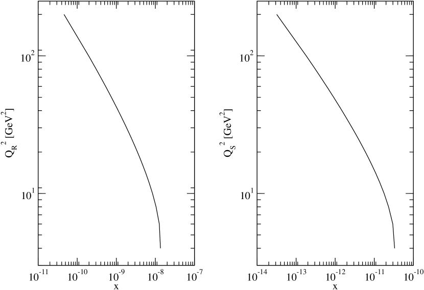
Figure 2: Recombination (left) and saturation (right) scales, defined according to Eqs. (18) and (19), determined using the PDFs of our previous work FAL2 .

From this table we realize that

1. the function $Q_{R}^{2}(x)$ is quite similar to the one obtained in Ref. ZAL with different values of the parameters (in particular the value of $K$ is quite different in our approach);

2. the recombination scale agrees with our findings for the $Q^{2}$ slope of $F_{2}^{\nu N}(x,Q^{2})$;

3. the evaluation we did of the neutrino-nucleon cross section is safe since the small-$x$ limit considered is well above the $x$-value associated with the recombination scale at $Q^{2}\sim M_{W}^{2}$; in other words higher order twists, besides twist-4, are not important.

This last point gives sense to a comparison of our results with those of Ref. JJM , where all twists were resummed, in the region of energy we considered.

As far as anti-shadowing effects are concerned, they are important at values of $Q^{2}$ much smaller that $M_{W}^{2}$ ZAL , therefore they are completely negligible in our analysis.

In conclusion we find that our approach is sound and reliable. It has many points in common with the analysis of Ref. JJM : saturation presents itself at very small $x$ and is not detectable, antishadowing is present in both approaches, but at different values of $Q^{2}$. Enhancement of ultra-high energy neutrino-nucleon cross section is not required in our calculation and this is due to the correlation among color sources in the target. Such correlation, and coherence, is absent in the color dipole picture.

Acknowledgments L.J. and A.K. thank the Departments of Physics of the Universities of Calabria and Padova, together with the INFN Gruppo collegato di Cosenza and Sezione di Padova for their warm hospitality and support. This work was partially supported by the Ministero Italiano dell’Istruzione, dell’Università e della Ricerca.

A Appendix: Proof of Eq. (15)

With the change of variable $t=\ln(Q^{2}/\Lambda^{2})$ we can rewrite the integral (14) in the following forms

$${\cal I}_{1}(d)\!\!\! = \!\!\!\frac{M_{W}^{4}}{\Lambda^{2}}\!\int_{\ln(Q_{0}^{2}/\Lambda^{2})}^{\ln(s/\Lambda^{2})}\frac{t^{-d}e^{t}\;dt}{\left(e^{t}+M_{W}^{2}/\Lambda^{2}\right)^{2}}$$

$$= \!\!\!\frac{M_{W}^{4}}{\Lambda^{2}}\!\left[\int_{\ln(Q_{0}^{2}/\Lambda^{2})}^{\ln(s/\Lambda^{2})}\frac{t^{-d}\;dt}{e^{t}+M_{W}^{2}/\Lambda^{2}}-\frac{M_{W}^{2}}{\Lambda^{2}}\int_{\ln(Q_{0}^{2}/\Lambda^{2})}^{\ln(s/\Lambda^{2})}\frac{t^{-d}\;dt}{\left(e^{t}+M_{W}^{2}/\Lambda^{2}\right)^{2}}\right]$$

$$= \!\!\!\frac{M_{W}^{4}}{\Lambda^{2}}\!\left[\int_{\ln(Q_{0}^{2}/\Lambda^{2})}^{\ln(s/\Lambda^{2})}\frac{t^{-d}e^{-t}\;dt}{1+M_{W}^{2}e^{-t}/\Lambda^{2}}-\frac{M_{W}^{2}}{\Lambda^{2}}\int_{\ln(Q_{0}^{2}/\Lambda^{2})}^{\ln(s/\Lambda^{2})}\frac{t^{-d}e^{-2t}\;dt}{\left(1+M_{W}^{2}e^{-t}/\Lambda^{2}\right)^{2}}\!\right]\!.$$

Setting $z=M_{W}^{2}/\Lambda^{2}$, we have

$${\cal I}_{1}(d) = M_{W}^{2}z\left(1+z\frac{d}{dz}\right)\int_{\ln(Q_{0}^{2}/\Lambda^{2})}^{\ln(s/\Lambda^{2})}\frac{t^{-d}e^{-t}\;dt}{1+ze^{-t}}$$ (A.1)

$$\equiv M_{W}^{2}z\left(1+z\frac{d}{dz}\right){\cal L}(d,z)\;.$$

${\cal L}(d,z)$ differs from the integral

$$\int_{\ln(Q_{0}^{2}/\Lambda^{2})}^{\infty}\frac{t^{-d}e^{-t}\;dt}{1+ze^{-t}}$$

by terms vanishing faster than $1/s$ in the asymptotic region for the variable $s$. This result can be easily obtained by expanding in series the integral in Eq. (A.1) with respect to its upper limit. Moreover, since $z$ is a large number ($\ln z\sim 12$ if $\Lambda=0.19$ GeV) another approximation becomes possible and, neglecting terms proportional to $[\ln(z)]^{-2}$ with respect to a constant term, we have

$${\cal L}(d,z)\simeq\int_{0}^{\infty}\frac{t^{-d}e^{-t}\;dt}{1+ze^{-t}}\;.$$ (A.2)

The integral (A.2) can be expressed as an infinite sum

$${\cal L}(d,z) \simeq \sum_{n=0}^{\infty}(-1)^{n}z^{n}\int_{0}^{\infty}dt\,t^{-d}e^{-(n+1)t}$$ (A.3)

$$= -\frac{1}{z}\Gamma(1-d)\,\sum_{n=1}^{\infty}\frac{(-z)^{n}}{n^{1-d}}$$

and finally

$${\cal L}\simeq-\frac{1}{z}\Gamma(1-d)F(-z,1-d)\;,$$ (A.4)

where $F(z,2)$ is the Euler’s dilogarithm. The analytical continuation of the series

$$F(-z,1-d)=\sum_{n=1}^{\infty}\;\frac{(-z)^{n}}{n^{1-d}}$$

is given by the Joncquière’s relation BAT that, in our case, becomes

$$F(-z,1-d)=-e^{i(1-d)\pi}F(-1/z,1-d)+\frac{(2\pi)^{1-d}}{\Gamma(1-d)}e^{i\pi(1-d)/2}\zeta\left(d,\frac{\ln(-z)}{2\pi i}\right).$$

The variable $z=M_{W}^{2}/\Lambda^{2}$ is very large and an asymptotic expansion for ${\cal L}$ follows from the asymptotic expansion of the generalized Zeta function for $z\to\infty$,

$$\zeta\left(d,\frac{\ln(-z)}{2\pi i}\right) \rightarrow \frac{1}{\Gamma(d)}\left[\Gamma(d-1)\left(\frac{\ln(-z)}{2\pi i}\right)^{1-d}\right.$$ (A.5)

$$+ \left.\frac{1}{2}\Gamma(d)\left(\frac{\ln(-z)}{2\pi i}\right)^{-d}+O\left(|\ln(z)|^{-1-d}\right)\right]\;.$$

Since

$${\cal I}_{1}(d) = M_{W}^{2}\Gamma(1-d)z\left(1+z\frac{d}{dz}\right)\Phi(-z,1-d,1)$$ (A.6)

$$= -M_{W}^{2}\Gamma(1-d)F(-z,-d)$$

and

$$-F(-z,-d)=\frac{1}{\pi}e^{-i\pi d/2}\Gamma(d)(-i\ln z)^{-d}\sin(\pi d)\;,$$ (A.7)

Eq. (15) follows at once.

B Appendix: Derivation of Eq. (17)

According to the modified DGLAP equations ZAL , we have

$$\frac{df_{q}^{full}(x,Q^{2})}{d\ln Q^{2}} = \frac{df_{q}(x,Q^{2})}{d\ln Q^{2}}+\frac{\alpha_{s}^{2}}{Q^{2}}K\left[\int^{x}_{x/2}\frac{dy}{y}F_{qg}\left(\frac{x}{y}\right)\left({f_{g}^{full}(y,Q^{2})}\right)^{2}\right.$$

$$- \left.\int_{x}^{1/2}\frac{dy}{y}F_{qg}\left(\frac{x}{y}\right)\left({f_{g}^{full}(y,Q^{2})}\right)^{2}\right]$$

$$\sim \frac{df_{q}(x,Q^{2})}{d\ln Q^{2}}+\frac{\alpha_{s}^{2}}{Q^{2}}K\left[\int^{x}_{x/2}\frac{dy}{y}F_{qg}\left(\frac{x}{y}\right)f_{g}^{2}(y,Q^{2})\right.$$

$$- \left.\int_{x}^{1/2}\frac{dy}{y}F_{qg}\left(\frac{x}{y}\right)f_{g}^{2}(y,Q^{2})\right]$$

$$\equiv \frac{df_{q}(x,Q^{2})}{d\ln Q^{2}}+\frac{\alpha_{s}^{2}}{Q^{2}}KR_{q}(x,Q^{2})\;.$$

Then, using Eqs. (28), (29) and (32) of Ref. FAL2 and recalling that we put $K_{1}=K_{2}$, we easily get

$$R_{q}(x,Q^{2}) \stackrel{{\scriptstyle M}}{{\to}} \Bigl{[}\tilde{F}_{qg}^{(r)}(n)-F_{qg}^{(r)}(n)\Bigr{]}\,f_{2}(n)-F_{qg}^{(r)}(n)\,f_{2}(n)$$ (B.2)

$$\stackrel{{\scriptstyle n\to 1}}{{=}} \left(\frac{131}{180}-2\,\frac{1813}{2880}\right)f_{2}(n)=-\frac{17}{32}f_{2}(n)$$

$$\stackrel{{\scriptstyle M^{-1}}}{{\to}} -\frac{17}{32}f_{g}^{2}(x,Q^{2})\;.$$ (B.3)

References

• [1] J.G. Learned and K. Mannheim, Ann. Rev. Nucl. Part. Sci. 50, 679 (2000).
• [2] G.M. Frichter, D.W. McKay and J.P. Ralston, Phys. Rev. Lett. 74, 1508 (1995); Erratum-ibid. 77, 4107 (1996).
• [3] R. Gandhi et al., Phys. Rev. D 58, 093009 (1998); Astropart. Phys. 5, 81 (1996).
• [4] J. Kwieciński, A.D. Martin and A.M. Staśto, Phys. Rev. D 59, 093002 (1999).
• [5] R. Fiore et al., Phys. Rev. D 68, 093010 (2003).
• [6] M. Reno, Nucl. Phys. Proc. Suppl. 143, 407 (2005).
• [7] K. Kutak and J. Kwieciński, Eur. Phys. J. C 29, 521 (2003).
• [8] M.V.T. Machado, Phys. Rev. D 70, 053008 (2004).
• [9] R. Fiore et al., Phys. Rev. D 71, 033002 (2005).
• [10] J. Jalilian-Marian, Phys. Rev. D 68, 054005 (2003); Erratum-ibid. 70, 079903 (2004).
• [11] I. Balitsky, Nucl. Phys. B 463, 99 (1996); Phys. Rev. Lett. 81, 2024 (1998); Phys. Lett. B 518, 235 (2001).
• [12] J. Jalilian-Marian et al., Nucl. Phys. B 504, 415 (1997); Phys. Rev. D 59, 014014 (1999).
E. Iancu, A. Leonidov and L.D. McLerran, Phys. Lett. B 510, 133 (2001); Nucl. Phys. A 692, 583 (2001).
• [13] E.M. Henley and J. Jalilian-Marian, hep-ph/0512220.
• [14] A.M. Stasto, K. Golec-Biernat and J. Kwieciński, Phys. Rev. Lett. 86, 596 (2001).
• [15] A.H. Mueller and D.N. Triantafyllopoulos, Nucl. Phys. B 640, 331 (2002); D.N. Triantafyllopoulos, ibidem 648, 293 (2003).
• [16] A.H. Mueller, Nucl. Phys. B 415, 373 (1994); ibidem 437, 107 (1995).
• [17] A. Kusenko and T.J. Weiler, Phys. Rev. Lett. 88, 161101 (2002).
• [18] W. Zhu, Nucl. Phys. B 551, 245 (1999); W. Zhu and J. Ruan, Nucl. Phys. B 559, 378 (1999).
• [19] W. Zhu et al., Phys. Rev. D 68, 094015 (2003)
• [20] V.N. Gribov and L.N. Lipatov, Sov. J. Nucl. Phys. 15, 438 (1972); Yu.L. Dokshitzer, Sov. Phys. JETP 46, 641 (1977).
• [21] G. Altarelli and G. Parisi, Nucl. Phys. B 126, 298 (1977).
• [22] Z. Shen and W. Zhu, Chin. Phys. Lett. 21, 1896 (2004).
• [23] A. Kovner and U.A. Wiedemann, Phys. Rev. D 66, 051502 (2002); ibidem, 034031 (2002).
• [24] Yu. Kovchegov, Phys. Rev. D 60, 034008 (1999).
• [25] Yu.M. Andreeev, V.S. Berezinsky and A. Yu. Smirnov, Phys. Lett. B 84, 247 (1979).
• [26] A. Buras, Rev. Mod. Phys. 52, 199 (1980).
• [27] C. Lopez and F.J. Ynduráin, Nucl. Phys. B 171, 231 (1980); ibidem 183, 157 (1981).
• [28] F. Martin, Phys. Rev. D 19, 1382 (1979).
• [29] A.V. Kotikov, Yad. Fiz. 57, 142 (1994) [Phys. Atom. Nucl. 57, 133 (1994)]; Phys. Rev. D 49, 5746 (1994).
• [30] A.V. Kotikov and G. Parente, Nucl. Phys. B 549, 242 (1999).
• [31] A.Yu. Illarionov, A.V. Kotikov and G. Parente, hep-ph/0402173.
• [32] L.V. Gribov, E.M. Levin and M.G. Ryskin, Phys. Rep. 100, 1 (1983).
• [33] J. Kwieciński, A.D. Martin, W.J. Stirling and R.G. Roberts, Phys. Rev. D 42, 3645 (1990) and references therein.
• [34] S. Chekanov et al, Phys. Rev. D 67, 012007 (2003).
• [35] Bateman Manuscript Project, Higher Transcendental Functions, Vol. II (McGraw-Hill 1954).