Survival probability for exclusive central diffractive production of colorless states at the LHC.

Abstract:

In this paper we discuss the survival probability for exclusive central diffractive production of a colorless small size system at the LHC. This process has a clear signature of two large rapidity gaps. Using the eikonal approach for the description of soft interactions, we predict the value of the survival probability to be about $5\sim 6\%$ for single channel models, while for a two channel model the survival probability is about $3\%$. The dependence of the survival probability factor (damping factor) on the transverse momenta of the recoiled protons is discussed, and we suggest it be measured at the Tevatron so as to minimize the possible ambiguity in the calculation of survival probability at the LHC.

1 Introduction

Following the pioneering papers of Ref.[1], it has been realized[2, 3] that large rapidity gaps (LRG) diffractive processes are suppressed due to the rescattering of the spectator partons. The calculations of the resulting gap survival probability (SP)[7, 6, 4, 5, 8, 9, 10] have since then been at the focus of high energy phenomenology. The incentive for this activity has been the need to obtain reliable SP estimates for Higgs diffractive production at the LHC. The analogous process of diffractive hard di-jet production has been measured at Fermilab[11] and HERA[12] and this may serve as a laboratory to check the validity and reliability of the proposed calculations.

SP is the probability to have a simple diffractive colorless final state configuration, in which the LRG are preserved, regardless of the strong interaction of the rescattered soft partons (see Fig. 1). Its calculation depends crucially on soft scattering physics, for which a theory is still lacking. The main phenomenological tool utilized in these calculations is the Regge soft Pomeron. In spite of the progress made in understanding the soft Pomeron structure within the framework of npQCD[13, 14, 15, 16, 17, 18, 19, 20, 21], we are still unable to predict the parameters associated with the phenomenological Pomeron[22], and to create a theory for soft scattering. Consequently, no theoretical approach exists which allows us to calculate a SP value to a specific given accuracy. As a substitute, the models which were developed utilize relatively simple soft Pomeron parametrizations and the rescattering process is approximated by eikonal-type models. These models satisfy the general principles of unitarity, including the Froissart and Pumplin bounds, and allows us to analyze the experimental data in accordance with these general principles.

At present, we can obtain only phenomenological estimates for SP. Although our calculations are applicable to any small size colorless system e.g. the production of Higgs mesons, in this paper we refer only to the particular case of a di-jet system, as there is experimental data from the Tevatron and HERA. In the simplest approach we have three steps in calculating the central hard exclusive production of a di-jet, $\,N+N\rightarrow N+LRG+JJ+LRG+N$, which is illustrated in Fig. 1.

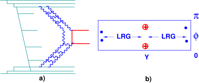
Figure 1: The contaminating soft rescatterings between partons, that produce secondaries which may fill the rapidity gaps (Fig. 1-a), and the lego-plot (Fig. 1-b) of our process. The probability that there are no additional soft interactions shown in Fig. 1-a, gives the survival probability for the diffractive di-jet production.

1) A description of the rescattering soft interactions. In the eikonal model, the elastic high energy amplitude is pure imaginary at high energy, and can be written in impact parameter b-space in the form (see, for example, Refs.[3, 6])

$$a_{el}\left(s;b\right)\,\, = \,\,i\,\left(\,1\,\,-\,\,e^{-\textstyle\frac{1}{2}\Omega(s,b)}\,\right),\,\,$$ (1.1)

$$G_{in}\left(s;b\right)\,\, = \,\,\,1\,\,-\,\,e^{-\Omega(s,b)}.\,\,$$ (1.2)

$s=W^{2}$, where $W$ is the c.m. energy of the initial hadronic collision, and $b$ is its impact parameter. For the opacity $\Omega$, we use the exchange of a soft Pomeron with a $t=0$ linear trajectory intercept of $(1+\Delta)$ and a slope $\alpha^{,}_{P}$. Accordingly,

$$\Omega(s,b)\,\,=\,\,\sigma_{0}\,\left(\,\frac{s}{s_{0}}\,\right)^{\Delta}\,S\left(s,b\right).$$ (1.3)

$S(s,b)$ denotes the b-space normalized soft profile function satisfying

$$\int\,\,d^{2}b\,S(s,b)\,=\,1.$$ (1.4)

In the framework of the eikonal model $\sigma_{0}$, $s_{0}$ and the form of the profile function are phenomenological inputs, extracted from the experimental data.
2) We need to find the impact parameter behaviour of the two hard Pomerons, that produce the di-jet in the central rapidity region, as is shown in Fig. 1-a. We denote this observable by $\frac{d^{2}\sigma_{H}}{d^{2}b}$. We can use the HERA DIS data to find this dependence. In this paper we will use the approach developed in Ref.[23], in which the b-dependence of the hard Pomeron has been extracted from the diffractive production of $J/\Psi$ meson in the HERA DIS experiments.
3) The third step is an actual calculation of the survival probability[2, 6]

$$<|S^{2}|>\,\,=\,\,\frac{\int\,\,d^{2}\,b\,\,\left(d\sigma_{H}/d^{2}b\right)\,\,\,\,e^{-\Omega(s,b)}\,}{\int\,\,d^{2}\,b\,\,\left(d\sigma_{H}/d^{2}b\right)}.$$ (1.5)

The interpretation of Eq. (1.5) derives from Eq. (1.2), where the factor $e^{-\Omega(s,b)}$ secures that no inelastic interactions occur which could change the LRG lego-plot of Fig. 1-b. However, the simple form of Eq. (1.5) is valid only for a single channel eikonal model in which only elastic rescatterings are considered. It needs to be modified in a more elaborate approach, such as two or three channel models, in which both elastic and diffractive rescatterings are included[7].

The above appealing sketch of the eikonal approach demonstrates, as well, the deficiencies which are inherent in all presently available models, even those which are more complicated than the eikonal rescattering approximation. As it stands, the first and the third steps are stricly phenomenological, and only the second step is based on well established pQCD. This shaky theoretical situation has been the main reason why we were not active in this field over the past five years. The strong current demand to evaluate the LHC diffractive cross sections and their SP, encouraged us to return to this subject.

This paper has two main goals. To begin with, we wish to calculate a range of possible values for exclusive LHC central di-jet (or Higgs) production. To this end, we employ the eikonal model, being simple and transparent, so that all uncertainties can be recognized and discussed. We wish to avoid more complicated calculations in which it is difficult to separate uncertainties in the values of the input parameters, from the qualitative behaviour of the amplitude (mostly as a function of the impact parameter b). We shall present and compare results stemmimg from a single channel eikonal model, utilizing two profile functions. A constituent quark model (CQM) recently suggested[30], and a two channel eikonal model[7].

Our second main goal is to assess the t-dependence of the calculated SP. The experimental study of this differential observable requires, obviously, a significantly higher statistics than presently available. However, as we shall see, the discovery potential associated with this information justifies both experimental and theoretical efforts.

In our approach we use three principles which alleviate our poor knowledge on soft scattering theory.
1) We aim to successfully describe the soft scattering data associated with our investigation. This includes the data base with which we adjust the input information for the construction of the eikonal opacity (or opacities) and the model predictions that can be tested experimentally.
2) Utilize all possible theoretical approaches to control our phenomenology. In particular, the pQCD calculation for the production of hard di-jets at short distances.
3) Even though the LHC is not yet running, we should present our overall LHC predictions so as to be a subject for an experimental test even at the preliminary runs, well before the survival probabilities can be experimentally assessed.

For a recent review on SP, see Ref.[24].

2 Formulation

In the following we present the main formulae pertinent to our investigations.

2.1 Basic formulae

Our elastic t-channel scattering amplitude is normalized so that

$$\frac{d\sigma}{dt}=\pi\;\mid f_{el}(s,t)\mid^{2},$$ (2.6)

$$\sigma_{tot}=4\pi\,Im\,f_{el}(s,0).$$ (2.7)

The amplitude in impact parameter space is given by

$$a_{el}(s,b)=\frac{1}{2\pi}\int d^{2}qe^{-i\vec{q}\cdot\vec{b}}f_{el}(s,t),$$ (2.8)

where, $t\,=\,-q^{2}$. In this representation we have

$$\sigma_{tot}\,\,\, = \,\,\,2\,\int\,d^{2}b\,\,\,\mbox{Im}\,a_{el}(s,b)\,,$$ (2.9)

$$\sigma_{el}\,\,\, = \,\,\,\int d^{2}b\,\,\mid a_{el}(s,b)\mid^{2}.$$ (2.10)

s-channel unitarity implies that $\mid a(s,b)\mid\leq 1$. When this is written in a diagonalized form we have

$$2\,\,\mbox{Im}\,a_{el}(s,b)\,\,=\,\,\mid a_{el}(s,b)\mid^{2}\,+\,G_{in}(s,b).$$ (2.11)

The corresponding inelastic cross section is written

$$\sigma_{in}\,\,=\,\,\int\,d^{2}b\,\,\,G_{in}(s,b).$$ (2.12)

$s$- channel unitarity is most easily enforced in the eikonal approach, where Eq. (1.1), Eq. (1.2) and Eq. (1.3) satisfy the unitarity constraint of Eq. (2.11).

2.2 The general expression for the survival probability

The amplitude for central hard di-jet production is shown in Fig. 2. $A_{H}$ denotes the exchange of a hard Pomeron responsible for the production of the two gluonic jets (or Higgs), at short distances. The amplitude $A_{S}$ includes all possible initial state interactions due to the exchange and interaction of soft Pomerons, including the possibility that the two initial nucleons do not interact.

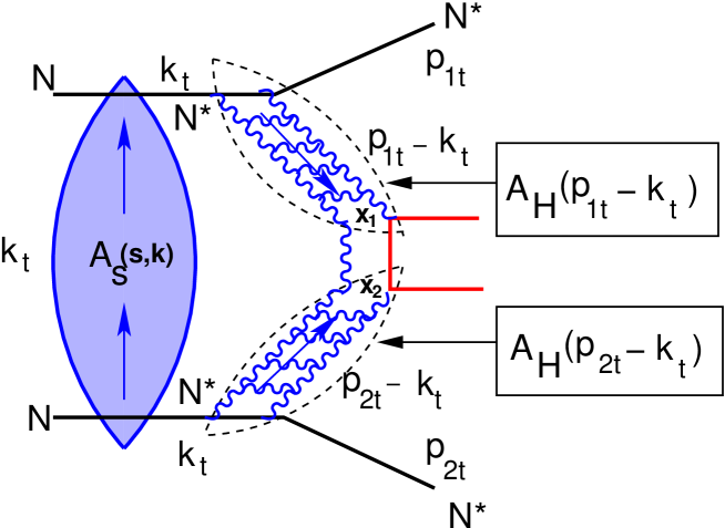
Figure 2: Central production of two hard jets separated by two large rapidity gaps from the accompanied final state nucleons and/or diffracted excited states (both are denoted by $N^{*}$). Possible rescattering of the initial two nucleons ($N$) is included.

The expression for the exclusive di-jet production (Fig. 2) has the form

$$A\left(N+N\,\,\to\,\,N\,+\,LRG\,+\,JJ\,+\,LRG\,+\,N\right)\,\,=$$ (2.13)

$$\,\,a_{hard}\,\int\,d^{2}\,k_{t}\,T_{H}\left((\vec{p}_{1t}-\vec{k}_{t})^{2};x_{1}\right)\,\,T_{H}\left((\vec{p}_{2t}-\vec{k}_{t})^{2};x_{2}\right)\,\,A_{S}\left(k^{2}_{t}\right)\,\,=\,\,$$

$$=\,\,A_{H}\,\,\int\,d^{2}\,b_{1}\,d^{2}b_{2}\,e^{i\,\vec{p}_{1t}\,\cdot\,\vec{b}_{1}\,+\,i\,\vec{p}_{2t}\,\cdot\,\vec{b}_{2}}A_{H}(b_{1})\,A_{H}(b_{2})\,\,A_{S}\left((\vec{b}_{1}\,+\,\vec{b}_{2})^{2}\right).$$

$a_{hard}$ is the amplitude for two hard Pomerons fusion into two jets. This process occurs at short distances, and we assume it to be independent of the impact parameters. $A_{H}$ is the amplitude for the hard Pomeron exchange, which is well known in pQCD[25, 26].

The full hard amplitude has a more complicated dependence and can be written as

$$T_{H}(p^{2}_{t},x)\,\,=\,\,A_{H}(p^{2}_{t})\,T_{H}(x)\,\,\longrightarrow\,A_{H}(b)\,T_{H}(x),$$ (2.14)

where the amplitude $T_{H}(x)$ absorbs the energy and transverse momenta dependence of the produced di-jet. We do not need to know the explicit dependence of these amplitude on energy and transverse momenta for our calculation of SP.

For the completeness of our presentation we introduce the factor $A_{hard}$ which has been calculated in Ref.[27]. This factor is given by

$$A_{hard}(HP+HP\rightarrow JJ)\,\,=\,\,\frac{32\pi}{9}\int^{P^{2}_{T}}\alpha_{S}(Q^{2})\,\frac{dQ^{2}}{Q^{4}}\,\phi(x_{1},Q^{2})\,\phi(x_{2}\,Q^{2})\,\,e^{-S(Q^{2},P^{2}_{T})}.$$ (2.15)

$HP$ denotes the hard Pomeron, $\phi$ is the unintegrated structure function and $\vec{P}_{T}\,=\,\frac{1}{2}(p_{1,t}+p_{2,t})$, where $p_{i,t}$ are the transverse momenta of the produced gluons. The Sudakov factor $e^{-S}$ secures that there is no radiation of gluons, with sufficiently large transverse momenta, from the exchanged gluons in Fig. 2. This suppression might be cosidered as a contribution to SP stemming from the hard sector. However, we note that it is included in the pQCD calculation of the hard process. See Ref.[27] for detailed calculations of $S$,$\phi$ and for the kinematical constraints for the process of di-jet production.

The most important characteristic of the hard Pomeron exchange for the calculation of the SP, is its dependence on the impact parameters. This dependence stems from the $b$-dependence of the proton-hard Pomeron vertex which can be defined in either BFKL[25] or DGLAP[26] approach. As we have mentioned, this dependence was extracted, in our calculation, from the DIS data[23], and we shall discuss it below.

$A_{S}$ is the amplitude accounting for the initial soft interaction, about which little is known. As stated, we start with a calculation of this amplitude in a single channel eikonal model. Accordingly, we consider only the elastic rescattering of the two initial nucleons, neglecting the summation over the possible excited nucleon states in Fig. 2.

For this cross section we have

$$\frac{d\sigma}{d^{2}p_{1t}\,d^{2}\,p_{2t},dy_{1}\,dy_{2}}\left(N+N\,\,\to\,\,N\,+\,LRG\,+JJ\,+\,LRG\,+N\right)\,\,=\,\,$$ (2.16)

$$=\,\,\sigma_{hard}\,\,|\int\,d^{2}\,b_{1}\,d^{2}b_{2}\,e^{i\,\vec{p}_{1t}\,\cdot\,\vec{b}_{1}\,+\,i\,\vec{p}_{2t}\,\cdot\,\vec{b}_{2}}A_{H}(b_{1})\,A_{H}(b_{2})\,\,A_{S}\left((\vec{b}_{1}\,+\,\vec{b}_{2})^{2}\right)|^{2},$$

where $p_{it}$ and $y_{i}$ are the transverse momenta and rapidities of the produced gluons (jets).

Integrating Eq. (2.16) over $p_{1t}$ and $p_{2t}$, we obtain the formula for SP (Eq. (1.5)) in the form

$$\langle\mid S\mid^{2}\rangle\,\,\,=\,\,\,\frac{\int\,d^{2}\,b_{1}\,d^{2}\,b_{2}\,\,\left[A_{H}(b_{1})\,A_{H}(b_{2})\,\,A_{S}\left((\vec{b}_{1}\,+\,\vec{b}_{2})^{2}\right)\right]^{2}}{\int\,d^{2}\,b_{1}\,d^{2}\,b_{2}\,\,\left[A_{H}(b_{1})\,A_{H}(b_{2})\right]^{2}}.$$ (2.17)

Let us introduce

$$\frac{d\sigma_{H}}{d^{2}\,b}\,\,\equiv\,\,\int\,d^{2}\,b^{\prime}\,\,A^{2}_{H}\left(\vec{b}-\vec{b}^{\,{}^{\prime}}\right)\,A^{2}_{H}(b^{\prime}),$$ (2.18)

and

$$e^{-\,\Omega(s,b)}\,\,\,\equiv\,\,A^{2}_{S}(b).$$ (2.19)

We find that Eq. (2.17) coincides with Eq. (1.5). We shall show below that Eq. (2.19) is a consequence of the eikonal model.

In the eikonal approximation the rescattering of two nucleons can be described by the set of diagrams presented in Fig. 3.

Figure 3: $A_{S}(b)$ in the eikonal model as a multi Pomeron exchange chain. ${\bf P}$ denotes the exchange of a soft Pomeron.

To understand the minus sign in front of the first rescattering term, one needs to substitute this diagram into Eq. (2.16), and remember that the single Pomeron exchange, as well as the diffractive production of jets, are pure imaginary. This leads to a negative contribution. See, for example, Ref.[28]. Summing all diagrams in Fig. 3, we obtain the eikonal formula for

$$A_{s}(b)\,\,\,=\,\,e^{-\textstyle\frac{1}{2}\,\Omega(s,b)},$$ (2.20)

which leads to Eq. (2.19). It is important to realize, in this context, that different LRG di-jet configurations, i.e. JGJ, GJJ and GJJG (which is discussed in this paper), have different $A_{s}(b)$ and intermediate states (see Fig. 5 and Eq. (2.56) below). Consequently, they have different SP values.

2.3 $A_{H}(b)$

To fix the impact parameter dependence of the hard amplitude, we return to the model of Ref.[23]. The t-dependence of the cross section for the diffractive production of $J/\Psi$ is shown in the diagram of Fig. 4.

Figure 4: t-dependence of $J/\Psi$ production in DIS.

The vertex for interaction of the hard Pomeron with the virtual photon leading to the production of $J/\Psi$, can be calculated in pQCD. From this calculation we can find the impact parameter dependence of the proton-hard Pomeron vertex. This vertex can be parameterized as an exponential in t

$$A_{H}(t)\,\,\,=\,\,e^{-\textstyle\frac{1}{2}B_{GG}\,|t|},$$ (2.21)

with $B_{GG}\,\,=\,\,3.6\,{\,\mbox{GeV}^{-2}}$[23]. The corresponding b-space transform of Eq. (2.21) is

$$A_{H}(b)\,\,\,=\,\,\,\frac{1}{\pi\,R^{2}_{H}}\,\exp\left(-\frac{b^{2}}{R^{2}_{H}}\right),$$ (2.22)

with $R^{2}_{H}\,=\,7.2\,{\,\mbox{GeV}^{-2}}$. In all our calculations below we take this form of $A_{H}(b)$.

Substituting Eq. (2.22) in Eq. (2.18) we obtain

$$\frac{d\sigma_{H}}{d^{2}\,b}\,\,=\,\,\frac{1}{\pi\,R^{2}_{H}}\,\,\exp\left(-\,\frac{b^{2}}{R^{2}_{H}}\right),$$ (2.23)

and

$$\int\,d^{2}\,b^{\prime}\,\,A_{H}\left(\vec{b}-\vec{b}^{\,{}^{\prime}}\right)\,A_{H}(b^{\prime})\,\,\,=\,\,\frac{2}{\pi\,R^{2}_{H}}\,\exp\left(-\,2\,\frac{b^{2}}{R^{2}_{H}}\right).$$ (2.24)

The uncertainties in the determination of $R_{H}$ are mostly related to the influence of the excited nucleons in the final state (see Fig. 2). To understand better the possible influence of these states on the value of SP, we consider the process of diffractive dissociation of the virtual photon to a $J/\Psi$ in CQM. In this model the hard Pomeron interacts with the constituent quark as it is shown in Fig. 2-b. The vertex of the hard Pomeron for this interaction is

$$V_{p\to 3q}\,\,=\,\,\int\,\prod_{i}d^{2}r_{i}\Psi_{N}(r_{1},r_{2},r_{3})\,e^{-q\,x_{1}}\,\Psi_{q}(r_{i}),$$ (2.25)

where $\Psi(r_{i})$ is the plane wave for the quark, and $\Psi_{N}$ is the wave function of the nucleon. This wave function actually depends on two variables. For example $r_{1,2}=r_{1}-r_{2}$ and $r_{3,1,2}=r_{3}-\textstyle\frac{1}{2}(r_{1}+r_{2})$. The elastic differential cross section is proportional to

$$|V_{p\to 3q}(t)|^{2}\,\,=\,\,\int\,d^{2}r_{1,2}\,d^{2}r_{3,1,2}\,|\Psi_{N}(r_{1,2},r_{3,1,2})|^{2}\,e^{i\vec{q}_{t}\cdot\vec{r}_{1,2}}\,\,\to\,\,$$ (2.26)

$$1\,\,+\,\,\,q^{2}\,\int\,d^{2}r_{1,2}\,d^{2}r_{3,1,2}\,r^{2}_{1,2}|\Psi_{N}(r_{1,2},r_{3,1,2})|^{2}\,\,+\,\,O(q^{4})=\,\,1\,+\,q^{2}\,<|r^{2}_{1,2}|>\,\,+\,\,O(q^{4}).$$

The value of $<|r^{2}_{1,2}|>$ can be evaluated from the $q=\sqrt{-t}$ behaviour of the elastic diffraction (see Fig. 2). This diagram leads to $A_{H}(t)$ of Eq. (2.21) given in the form

$$A_{H}(t)\,\,=\,\,\int\,d^{2}r_{1,2}\,d^{2}r_{3,1,2}\,|\Psi_{N}(r_{1,2},r_{3,1,2})|^{2}\,e^{i\frac{2}{3}\vec{q}_{t}\cdot\vec{r}_{3,1,2}}\,\,\to\,\,1\,\,+\,\,\frac{4}{9}\,<|r^{2}_{1,2}|>\,\,+\,\,O(q^{4}).$$ (2.27)

Therefore, $B_{GG}\,\,=\,\,\frac{8}{9}<|r^{2}_{1,2}|>$ . Adding the combinatorial factors, we see that the t-dependence of the differential cross section for diffractive $J/\Psi$ production is given by

$$\frac{d\sigma(\gamma^{*}+p\to J/\Psi+3q)}{dt}\,\,\propto\,\,6\,\exp\left(-\frac{9}{8}\,B_{GG}\,|t|\right)\,\,\,+\,\,3\,\exp\left(-\,B^{in}_{GG}\,|t|\right),$$ (2.28)

where the second term originates from the elastic rescattering off one quark. Using the same procedure to extract the slope $B^{in}_{GG}$ from $B_{in}$ in Fig. 4, we estimate $B^{in}_{GG}\,\,=\,\,1\,\,{\,\mbox{GeV}^{-2}}$.

Eq. (2.23) has, thus, the form

$$\frac{d\sigma_{H}}{d^{2}\,b}\,\,=\,\,\frac{1}{9}\,\left(\,4\,\frac{1}{\pi\,2\,B_{GG}}\,\,\exp\left(-\,\frac{b^{2}}{2B_{GG}}\right)\,\,+\,\,4\,\frac{1}{\pi\,\,(B_{GG}\,+\,B^{in}_{GG})}\,\,\exp\left(-\,\frac{b^{2}}{B_{GG}\,\,+\,\,B^{in}_{GG}}\right)\,\,+\right.$$

$$\left.\,\,\frac{1}{\pi\,2\,B^{in}_{GG}}\,\,\exp\left(-\,\frac{b^{2}}{2B^{in}_{GG}}\right)\right).$$ (2.29)

2.4 Modelling the impact parameter dependence of the soft scattering amplitude

In the eikonal model the opacity $\Omega$ corresponds to a single soft Pomeron exchange. The t-dependence of this contribution is

$$\Omega\,\,=\,\,\sigma_{0}\,V^{2}_{N}(t)\,\left(\frac{s}{s_{0}}\right)^{\Delta\,-\,\alpha^{\prime}_{P}\,|t|},$$ (2.30)

where $V_{N}(t)$ is the proton-soft Pomeron vertex with the normalization $V(t=0)=1$.

We will use two simple models for the t-dependence of the vertex $V_{N}(t)$.
1) An exponential parametrization valid in the forward t-cone.

$$V_{N}(t)\,\,=\,\,\exp\left(-\frac{B_{0,el}}{4}\,|t|\right),$$ (2.31)

where $B_{0,el}$ is the exponential slope of the elastic differential cross section due to a soft Pomeron exchange at $s=s_{0}$. Although there is no theoretical justification for it, the parametrization suggested in Eq. (2.31), is in accord with all experimental observables, that are sensitive to the small t region. In the following it will be denoted GP.
2) A parametrization more suitable to cover a wider t range, including the diffractive dips observed in $\frac{d\sigma_{el}}{dt}$ is

$$V_{N}(t)\,\,=\,\,G_{N}(t).$$ (2.32)

$G_{N}(t)$ is the proton electromagnetic form factor (see for example Ref.[22]). We will use the dipole parameterization for this form factor

$$G_{N}(t)\,\,\,=\,\,\,\frac{1}{(1+t/m^{2})^{2}}\,,$$ (2.33)

with $m^{2}=0.72\,{\,\mbox{GeV}^{2}}$. The above parametrization is used in CQM.

The profile functions corresponding to GP and PP have the form

$$S_{GP}(s,b)\,\, = \,\,\frac{1}{2\pi\,B_{el}}\,\exp\left(-\frac{b^{2}}{2B_{el}}\right),$$ (2.34)

with $B_{el}\,\,=\,\,B_{0,el}\,\,+\,\,2\,\alpha^{\prime}_{P}\,\ln(s/s_{0})$.

$$S_{PP}(s,b)\,\, = \,\,\,\int\,q\,d\,q\,J_{0}\left(q\,b\right)\,G^{2}_{N}(t)\,\,\,\exp\left(-\,\,\alpha^{\prime}_{P}\,\ln(s/s_{0})\,\,\,q^{2}\,\right).$$ (2.35)

2.5 Explicit analytic formulae for the Gaussian parametrization

Using the parameterization of Eq. (1.1), Eq. (1.2), Eq. (1.3) and Eq. (2.34)) for the soft profile function, we can obtain simple analytic expressions for the main observables of the soft interaction [6].

$$\sigma_{tot} = 2\int d^{2}b(1-e^{-\Omega(s,b)/2})=4\pi B_{el}(s)\left[ln(\frac{\nu(s)}{2})+C-Ei(-\frac{\nu(s)}{2})\right],$$ (2.36)

$$\sigma_{in} = \int d^{2}b(1-e^{-\Omega(s,b)})=2\pi B_{el}(s)\left[ln(\nu(s))+C-Ei(-\nu(s))\right],$$ (2.37)

$$\sigma_{el} = \sigma_{tot}-\sigma_{in}=2\pi B_{el}(s)\left[ln(\frac{\nu(s)}{4})+C+Ei(-\nu(s))-2Ei(-\frac{\nu(s)}{2})\right],$$ (2.38)

$$\sigma_{el}/\sigma_{tot} = \textstyle\frac{1}{2}\left[ln(\frac{\nu(s)}{4})+C+Ei(-\nu(s))-2Ei(-\frac{\nu(s)}{2})\right]/\left[ln(\frac{\nu(s)}{2})+C-Ei(-\frac{\nu(s)}{2})\right],$$ (2.39)

where

$$\nu(s)\,\,=\,\,\Omega(s,b=0),$$ (2.40)

$Ei(x)=\int_{-\infty}^{x}\frac{e^{t}}{t}dt$ and C = 0.5773. From Eq. (2.39) we note that the ratio of $\sigma_{el}/\sigma_{tot}$ depends only on the value of $\nu(s)$ and, therefore, provides a possibility to find the value of $\nu$ directly from the experimental data[6].

The SP, given by Eq. (1.5), can also be calculated analytically if we assume Eq. (2.23) for $d\sigma_{H}(b)/d^{2}b$. We obtain

$$\langle\mid S\mid^{2}\rangle\,\,=\,\,\,\frac{a(s)\gamma\left(a(s),\nu(s)\right)}{\left[\nu(s)\right]^{a(s)}}.$$ (2.41)

The incomplete gamma function is $\gamma(a,x)=\int_{0}^{x}z^{a-1}e^{-z}dz$ and $a(s)\,=\,\frac{2\,B_{el}(s)}{R^{2}_{H}(s)}$. For the profile function of Eq. (2.35) we cannot provide a set of analytic formulae. We have used the above formulae as a check of our methods and numerical computations.

2.6 Constituent quark model

The characteristics of the soft processes can be alternatively calculated also with CQM[30]. In CQM we assume that all hadrons consist of constituent quarks (two for a meson and three for a baryon), and all scattering processes go through the interactions of the constituent quarks. In this model the state of three free quarks diagonalizes the interaction matrix, the proton state, and the diffraction dissociation state, which can be viewed as the expansion of the three quark plane wave function

$$\prod_{i=1}^{3}\,\,\Psi_{q}(r_{i})\,\,=\,\,\alpha\,\Psi_{p}\,\,+\,\,\beta\,\Psi_{D},$$ (2.42)

with a normalization $\alpha^{2}\,+\,\beta^{2}\,=\,1$. The constituent quark model can be viewed, thus, as a particular realization of a two channel model which we will consider below on a more general basis.

For a constituent quark-quark scattering amplitude we use the eikonal formulae Eq. (1.1) and Eq. (1.2). Accordingly, the amplitude for the scattering of a quark $i_{1}$ from the first hadron with a quark $i_{2}$ from the second hadron is

$$A_{i_{1},i_{2}}(s,b)\,\,=\,\,i\,\left(\,1\,\,-\,\,\exp\left(-\frac{\Omega_{i_{1},i_{2}}(s,b)}{2}\right)\,\right).$$ (2.43)

The opacity $\Omega_{i_{1},i_{2}}$ is given by

$$\Omega_{i_{1},i_{2}}^{CQM}\,\,=\,\,\,$$ (2.44)

$$\,\,\frac{\sigma_{0}}{\pi\,\left(8\,B^{in}_{GG}\,\,+\,\,4\,\alpha^{\prime}_{P}\,\ln(s/s_{0})\right)}\,\,\,\left(\,\frac{s}{s_{0}}\,\right)^{\Delta}\,\,\exp\left(-\frac{b^{2}_{i_{1},i_{2}}}{8\,B^{in}_{GG}\,\,+\,\,4\,\alpha^{\prime}_{P}\,\ln(s/s_{0})}\,\right),$$

where $\vec{b}_{i_{1},i_{2}}\,\,=\,\,\vec{r}_{i_{1},k_{1},l_{1}}\,\,=\,\,\vec{r}_{i_{1}}\,\,-\,\,\textstyle\frac{1}{2}(\vec{r}_{k_{1}}+\vec{r}_{l_{1}})$.

In this paper we simplify Eq. (2.44) assuming that $b\,\,\gg\,\,r_{i_{1},k_{1},l_{1}}\approx\,r_{i_{2},k_{2},l_{2}}$. It is certainly correct at very high energies, since $b^{2}\,\,\propto\,\,4\,\alpha^{\prime}_{P}\,\ln(s/s_{0})\,\,\gg\,\,r^{2}_{i_{1},k_{1},l_{1}}$. More advanced calculations in the framework of CQM have been presented in Ref.[30].

Having defined the opacities, we obtain the following formulae for the soft cross sections

$$\sigma_{tot}\,\, = \,\,9\,\,\times\,\,2\,\int\,d^{2}b\,\left(\,1\,-\,\exp\left(\,-\textstyle\frac{1}{2}\,\Omega^{CQM}(s,b)\right)\right),$$ (2.45)

$$d\,\sigma_{el}/dt\,\, = \,\,9^{2}\,\,\times\,\,G^{4}_{N}(t)\,|f^{CQM}(s,t)|^{2}\,,$$ (2.46)

$$d\,\sigma_{diff}/dt+d\,\sigma_{el}/dt\,\, = \,\,9^{2}\times\,\,\left(\frac{2}{3}\exp\left(-\frac{9}{8}\,[B_{GG}\,-\,B^{in}_{GG}]\,|t|\right)+\frac{1}{3}\,\,\right)^{2}\,\,|f^{CQM}(s,t)|^{2}\,\,.$$ (2.47)

$f^{CQM}(s,t)$ is the quark-quark scattering amplitude in the t-representation, see Eq. (2.6) and Eq. (2.8) for the relations between t and b representations. $G_{N}(t)$ is the electro-magnetic proton form factor (see Eq. (2.33)). The numerical combinatorial factors give the number of interacting quark-quark (antiquark) pairs. Note that in the CQM diffraction is confined to small masses[30].

In CQM, with $d^{2}\sigma_{H}/d^{2}b$ given by Eq. (2.29), we obtain

$$<|S^{2}|>\,\,=\,\,\frac{\int\,\,d^{2}\,b\,\,\left(d\sigma_{H}/d^{2}b\right)\,\,\,\,e^{-9\,\cdot\Omega_{i_{1},i_{2}}(s,b)}}{\int\,\,d^{2}\,b\,\,\left(d\sigma_{H}/d^{2}b\right)},$$ (2.48)

where $\Omega_{i_{1},i_{2}}$ is determined by Eq. (2.44). Eq. (2.48) determines the probability that none of the possible nine quark-quark pairs can rescatter inelastically leading to the production of additional hadrons.

Comparing the calculations using this model with the calculations using the eikonal approach, we are able to assess how sensitive the value of SP is to a more elaborate model.

2.7 Two channel model

A major deficiency of the single channel eikonal model is its failure to reproduce the observed mild energy dependence of $\sigma_{sd}$ in the ISR and above[3]. In a single channel model, $\sigma_{sd}$ is assumed to be small enough so that $\frac{\sigma_{sd}}{\sigma_{el}}$ is a small parameter. Hence, the eikonal rescatterings are elastic. Accordingly, $\sigma_{sd}$ is not included in the fitted data base fixing the single channel model parameters. Regardless, the SP of $\sigma_{sd}$ can be calculated resulting with disappointing output. The model’s inability to reproduce the diffractive cross section energy dependence reflects an over estimation of SP at higher energies (see Ref.[3] for details).

To overcome this difficulty we have developed a more elaborate multi channel eikonal model[7] in which both elastic and diffractive soft rescatterings are included resulting in a decrease of the calculated high energy SP. In the two channel version of the model double diffraction is assumed to be small enough so as to be neglected in the eikonal rescatterings. This assumption is supported by the data available in the ISR-Tevatron range. Note that the addition of a competing diffractive channel actually reduces the elastic screening. In our model, the added diffractive screening adds more screening than the loss it has induced. The final results in an over all larger screening which reproduces the SD data well, considering the scatter of the experimental points[24].

In a two channel model, the two hadron states of a proton and a diffractive state are considered simultaneously.

$$\Psi_{p}\, = \,\alpha\,\Psi_{1}\,\,+\,\,\beta\,\Psi_{2}\,\,,$$ (2.49)

$$\Psi_{D}\, = -\,\beta\,\Psi_{1}\,\,+\,\,\alpha\,\Psi_{2}\,\,.$$ (2.50)

p and D denote the proton (Eq. (2.49)) and diffractive (Eq. (2.50)) states. The wave functions functions $\Psi_{1}$ and $\Psi_{2}$ are orthogonal. They diagonalize the interaction matrix at high energies and, therefore,

$$A^{i\rightarrow j}_{k\rightarrow l}\,\,=\,\,A_{i,k}\,\delta_{i,j}\,\delta_{k,l}\,.$$ (2.51)

As in the single channel formulation

$$A_{i,k}\,\,=\,\,i\left(\,1\,\,-\,\,e^{-\textstyle\frac{1}{2}\Omega_{i,k}}\,\right).$$ (2.52)

For the opacities $\Omega_{i,k}(b)$ we use a GP parameterization

$$\Omega_{i,k}(b)\,\,=\,\,\nu_{i,k}\,e^{-\frac{b^{2}}{R^{2}_{i,k}}}\,=\,\frac{\sigma^{0}_{i,k}}{\pi\,R^{2}_{i,k}(s)}\,\left(\frac{s}{s_{0}}\right)^{\Delta}\,\,e^{-\frac{b^{2}}{R^{2}_{i,k}}},$$ (2.53)

where $\left(\sigma^{0}_{i,k}\right)^{2}\,=\,\sigma^{0}_{i,i}\,\sigma^{0}_{k,k}$ and

$$R^{2}_{i,k}(s)\,=\,2\,R^{2}_{i,0}\,+\,2\,R^{2}_{k,0}\,\,+\,\,4\,\alpha^{\prime}_{P}\,\ln(s/s_{0}).$$ (2.54)

More details regarding the parametrization can be found in Ref.[7]. An important fitted parameter which is essential for the present study is $\beta=0.464$.

For the calculation of exclusive di-jet central production SP we need to generalize Eq. (1.5) for a two channel scenario. This generalization is illustrated in Fig. 5, leading to a generalization of Eq. (2.13)

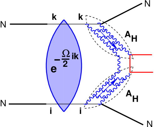
Figure 5: Production of di-jet with two large rapidity gaps in the two channel eikonal model for the soft interaction.

$$A\left(N+N\,\,\to\,\,N\,+\,LRG\,+JJ+\,LRG\,+N\right)\,\,=$$ (2.55)

$$=\,\,a_{hard}\,\,\sum_{i,k}\int\,d^{2}\,b_{1}\,d^{2}b_{2}\,e^{i\,\vec{p}_{1t}\,\cdot\,\vec{b}_{1}\,+\,i\,\vec{p}_{2t}\,\cdot\,\vec{b}_{2}}A_{H}(i\to p;b_{1})\,A_{H}(k\to p;b_{2})\,\,e^{-\frac{\Omega_{i,k}\left((\vec{b}_{1}\,+\,\vec{b}_{2})^{2}\right)}{2}}.$$

This equation can be rewritten in an explicit way using Eq. (2.49) (see Refs.[7, 24] for details).

$$A\left(N+N\,\,\to\,\,N\,+\,LRG\,+JJ+\,LRG\,+N\right)\,\,=$$ (2.56)

$$=\,\,a_{hard}\,\,\int\,d^{2}\,b_{1}\,d^{2}b_{2}\,e^{i\,\vec{p}_{1t}\,\cdot\,\vec{b}_{1}\,+\,i\,\vec{p}_{2t}\,\cdot\,\vec{b}_{2}}\,\left(\alpha^{2}\,e^{-\frac{-\Omega_{1,1}\left((\vec{b}_{1}\,+\,\vec{b}_{2})^{2}\right)}{2}}\,A_{H}(1\to p;b_{1})\,A_{H}(1\to p;b_{2})\,\,\right.$$

$$\left.+\,\,\alpha\,\beta\,e^{-\frac{-\Omega_{1,2}\left((\vec{b}_{1}\,+\,\vec{b}_{2})^{2}\right)}{2}}\,\{A_{H}(1\to p;b_{1})\,A_{H}(2\to p;b_{2})\,+\,A_{H}(2\to p;b_{1})\,A_{H}(1\to p;b_{2})\}\right.$$

$$\left.\,+\,\beta^{2}\,\,e^{-\frac{-\Omega_{2,2}\left((\vec{b}_{1}\,+\,\vec{b}_{2})^{2}\right)}{2}}\,A_{H}(2\to p;b_{1})\,A_{H}(2\to p;b_{2})\right).$$

Eq. (2.56) can be written in a more convenient form which enables us to use the experimental data corresponding to Fig. 4. We introduce two amplitudes

$$A_{H}(p\to p;b)\,\, = \frac{V_{p\to p}}{2\pi B_{GG}}\,\,\exp\left(-\frac{b^{2}}{2\,B_{GG}}\right)\,,$$ (2.57)

$$A_{H}(p\to D;b)\,\, = \,\,\frac{V_{p\to D}}{2\pi B^{in}_{GG}}\,\,\exp\left(-\frac{b^{2}}{2\,B^{in}_{GG}}\right)\,,$$ (2.58)

where the input parameters $B_{GG}$ and $B^{in}_{GG}$ have been introduced in Section II.C. The input assumption of the two channel model[7] is that the double diffractive production is small enough to be neglected. Using this assumption, together with Eq. (2.57), Eq. (2.58), Eq. (2.49) and Eq. (2.50), enables us to rewrite Eq. (2.56)

$$A\left(N+N\,\,\to\,\,N\,+\,LRG\,+JJ+\,LRG\,+N\right)\,\,=$$ (2.59)

$$=\,\,a_{hard}\,\,\int\,d^{2}\,b_{1}\,d^{2}b_{2}\,e^{i\,\vec{p}_{1t}\,\cdot\,\vec{b}_{1}\,+\,i\,\vec{p}_{2t}\,\cdot\,\vec{b}_{2}}\,\,\exp\left(-\frac{-\Omega\left((\vec{b}_{1}\,+\,\vec{b}_{2})^{2}\right)}{2}\right)\,\,$$

$$\left(\left(1-2\,\beta^{2}s_{D}\left((\vec{b}_{1}\,+\,\vec{b}_{2})^{2}\right)\right)\,A_{H}(p\to p;b_{1})\,A_{H}(p\to p;b_{2})\right.$$

$$\left.\,-\,\,2\,\alpha\,\beta\,\,s_{D}\left((\vec{b}_{1}\,+\,\vec{b}_{2})^{2}\right)\,\{\,A_{H}(p\to p;b_{1})\,A_{H}(p\to D;b_{2})\,\,+\,\,A_{H}(p\to D;b_{1})\,A_{H}(p\to p;b_{2})\right).$$

In our notation

$$s_{D}(b)\,\,=\,\,1\,\,-\,\,\exp\left(-\frac{\Delta\Omega(b)}{2}\right),$$ (2.60)

with $\Delta\Omega(b)=\Omega_{1,2}-\Omega_{1,1}$.

For the opacities $\Omega$ and $\Delta\Omega$ we use the forms and fitted parameter values of Ref.[7].

$$\Omega(b)\,\, =\,\,\frac{\sigma_{0,p}}{\pi\,R^{2}_{p}(s)}\,\left(\frac{s}{s_{0}}\right)^{\Delta}\,\exp\left(-\frac{b^{2}}{R^{2}_{p}(s)}\right)\,,$$ (2.61)

$$\Delta\Omega(b)\,\, =\,\,\frac{\sigma_{0,D}}{\pi\,R^{2}_{D}(s)}\,\left(\frac{s}{s_{0}}\right)^{\Delta}\,\exp\left(-\frac{b^{2}}{R^{2}_{D}(s)}\right)\,,$$ (2.62)

where

$$R^{2}_{p\,or\,D}\,\,\,=\,\,R^{2}_{0,p\,or\,D}\,\,\,+\,\,4\,\alpha^{\prime}_{P}\,\ln(s/s_{0}).$$ (2.64)

Note that $R^{2}_{0,D}\,=\,\frac{1}{2}R^{2}_{0,p}$.

To obtain the SP we need to substitute the following two elements in Eq. (1.5).

$$\frac{d\sigma_{H}}{d^{2}b}\,\,\longrightarrow\,T^{H}_{el}(b),$$ (2.65)

and

$$e^{-\Omega}\,\frac{d\sigma_{H}}{d^{2}b}\,\,\longrightarrow\,\,e^{-\Omega}\,\,\left((1-2\,\beta^{2}s_{D})^{2}\,T^{H}_{el}(b)\,\,\right.$$ (2.66)

$$\left.-\,\,4\,\,v\,\alpha\,\beta(1-2\,\beta^{2}s_{D})\,s_{D}\,T^{H}_{1}(b)\,\,+\,\,8\,v^{2}\,\alpha^{2}\,\beta^{2}\,s^{2}_{D}\,\{\,T^{H}_{2}(b)\,+\,\,T^{H}_{3}(b)\}\right).$$

$v\,=\,V_{p\to D}/V_{p\to p}$, and

$$T^{H}_{el}\,\, = \,\frac{1}{2\,\pi\,B_{GG}}\,\exp\left(-\frac{b^{2}}{2B_{GG}}\right)\,,$$ (2.67)

$$T^{H}_{i}\,\, = \,\frac{1}{\pi\,B^{H}_{i}}\,\exp\left(-\frac{b^{2}}{B^{H}_{i}}\right)\,.$$ (2.68)

The corresponding input slopes are

$$B^{H}_{1}\,\, = \,\frac{1+3\kappa}{1+\kappa}\,B_{GG}\,,$$ (2.69)

$$B^{H}_{2}\,\, = \,(1+\kappa)\,B_{GG}\,,$$ (2.70)

$$B^{H}_{3}\,\, = \,\frac{4\kappa}{1\,+\,\kappa}\,B_{GG}\,,$$ (2.71)

where $\kappa=B^{in}_{GG}/B_{GG}$.

3 Results and Comparisons

In this section we present the results of the four models we have considered and compare them with the relevant experimental data. We then proceed to present and assess our SP predictions aiming to define a value and a range for the SP of a central GJJG exclusive dijet production at the LHC.

3.1 Adjusted parameters

Following is a summary of the phenomenological adjusted parameters for the soft input of the four models we have considered.

$$\mbox{The intercept of the soft Pomeron trajectory at}\,\,t=0 \Delta\,,$$ (3.72)

$$\mbox{The slope of the soft Pomeron trajectory at}\,\,t=0 \alpha^{\prime}_{P}\,,$$ (3.73)

The initial energy squared $$s_{0}\,,$$ (3.74)

$$\mbox{The strength of the Pomeron interaction at}\;s=s_{0}\,\, \sigma_{0}\,,$$ (3.75)

$$\mbox{The slope of the vertex}\;V_{N}(t)\,\, B_{0,el}\,,$$ (3.76)

The slope of the vertices in the two channel model $$R^{2}_{0,p}\,\,\mbox{and}\,\,R^{2}_{0,D}\,,$$ (3.77)

$$\mbox{The fraction of}\,\Psi_{D}\,\mbox{and}\,\Psi_{2} \beta\,.$$ (3.78)

We determine these parameters by fitting the value and energy dependence of the soft data base observables. As previously mentioned, the input assumption of a single channel eikonal model is that $\frac{\sigma_{diff}}{\sigma_{el}}<<1$. Accordingly, its data base consists of $\sigma_{tot}$, $\sigma_{el}$ and $B_{el}$, whereas $\sigma_{sd}$ is a prediction. CQM parameters are adjusted from the same data base. Since this model applies only to small mass diffraction[30], it cannot predict $\sigma_{sd}$. The data base for the two channel model includes the above and in addition the $\sigma_{sd}$ data points. We calculate the corresponding SP as a prediction derived after fixing these parameters, provided we can specify the opacity (opacities) of the screened hard process.

The best fit adjusted parameters for the models considered are presented in Table I. Note that even though the fitted $\sigma_{0}$ values obtained for the single channel model GP and PP profiles are identical, the corresponding $\nu$ values are different reflecting different b-distributions.

Parameters	$\Delta$	$\alpha^{\prime}_{P}(0)$	$s_{0}$	$\sigma_{0}$	Slope
Gaussian parameterization
(GP, Eq. (2.34))	0.09	0.25${\,\mbox{GeV}^{-2}}$	450 ${\,\mbox{GeV}^{2}}$	47.2  mb	$B_{0,el}$ =  10.24  ${\,\mbox{GeV}^{-2}}$
Power -like parameterization
(PP, Eq. (2.35))	0.09	0.25${\,\mbox{GeV}^{-2}}$	450 ${\,\mbox{GeV}^{2}}$	47.2   mb	$m^{2}$ = 0.72 ${\,\mbox{GeV}^{-2}}$
Constituent Quark Model
(CQM, Eq. (2.44)-Eq. (2.47))	0.08	0.28${\,\mbox{GeV}^{-2}}$	250 ${\,\mbox{GeV}^{2}}$	4.13 mb	$B^{in}_{GG}$ =  0.5 ${\,\mbox{GeV}^{-2}}$
Two channel model
2ChM $\beta\,=\,0.464$	0.126	0.2 ${\,\mbox{GeV}^{-2}}$	1  ${\,\mbox{GeV}^{2}}$	5.07 mb ($\sigma^{0}_{p}$)	16.34 ${\,\mbox{GeV}^{-2}}$ ($R^{2}_{0,p}$)
(Eq. (2.49) - Eq. (2.53))				56.5 mb ($\sigma^{0}_{D}$)	8.17 ${\,\mbox{GeV}^{-2}}$ ($R^{2}_{2,D}$)

Table 1: The best fit adjusted values of the Pomeron parameters in the models considered.

3.2 Reproduction of the soft scattering observables

A quality reproduction of $\sigma_{tot}$, $\sigma_{el}$ and $B_{el}$ is an obvious prerequisite for a soft scattering model with which we may calculate the SP of interest. As we noted, $\sigma_{sd}$ is not included in the soft data base of the single channel eikonal model, but it is a prediction of the model[3]. CQM is not suitable to calculate $\sigma_{sd}$. In the two channel model, $\sigma_{sd}$ is included in the fitted data base. In the following we discuss the details of the soft scattering output of the models we have considered.

3.2.1 One channel model

For the purpose of our present investigation we have considered a toy soft DL like[22] Pomeron exchange model, neglecting the secondary Regge exchanges. This is a strictly high energy model for which we take, never the less, a relatively low $s_{0}\,=\,450\,{\,\mbox{GeV}^{2}}$. This choice should be compared with standard Regge pole parametrizations in which the Regge contribution diminishes at much higher energies. Consequently, this model can not be continued to lower energies. The best adjusted Pomeron parameters are given in Table I. Regardless of its simplicity, this model provides a very reasonable reproduction of its data base in the ISR-Tevatron enery range. An interesting observation is that the two profiles result in remarkably close outputs. This is so even though the $\nu$ values corresponding to the two profiles are quite different. $\nu_{GP}(450)=1.88$, while $\nu_{PP}(450)=2.31$. We conclude that a good reproduction of the data base requires a delicate compensation between $\nu$ and the effective radius of the two profiles respectively.

Checking the b-distribution output of a given eikonal model, we encounter a fundamental feature, which is very transparent in the single channel version with a GP profile input for both the elastic and diffractive amplitudes. The elastic amplitude output, which respects unitarity, maintains an approximate Gaussian b-distribution peaking at b = 0. On the other hand, the diffractive amplitude output is non Gaussian peaking at a non zero b. The sum of the two amplitudes respects the Pumplin bound. This phenomena is easily understood once we note that the eikonalization of a diffractive amplitude amounts to the transition $M_{diff}(s,b)\rightarrow M_{diff}(s,b)e^{-\Omega(s,b)}$. Since $\Omega$ is central its suppressing effect is maximal at small b, and diminishes at high b (For details see Ref.[6, 7] and the preprint first version of this paper [31]).

As noted, the problematic asset of the single channel model is its inability to reproduce the energy dependence of $\sigma_{sd}$, which implies an over estimation of the corresponding SP becoming worse with increasing energy. As a result, we consider any SP calculated within the single channel to represent, at best, an upper limit for the SP.

3.2.2 CQM

The CQM does not provide a good reproduction of the soft data base at low and medium energies. It is applicable for the Tevatron energies and above. Note that in this model the PP profile is naturally related the electro-magnetic form factor of the proton. CQM is limited to small mass diffraction only, since the triple Pomeron vertex is not included in its formulation. Consequently, $\sigma_{sd}$ is not included in its soft data base. Since the model takes into account the rescatterings due to low mass exitation of the interacting hadrons it may be classified as an example of a simple two channel model.

The advantages of the model is it simplicity and the realistic b-dependence. The model does enable us a calculation of low mass $\frac{d\sigma_{diff}}{dt}$/$\sigma_{diff}$ presented in Fig. 6 at LHC energy. The positions of the calculated dips are a consequence of the input PP profile and should be considered reasonably reliable since the model, with this input, correctly reproduces the t dependence of the Tevatron elastic cross sections.

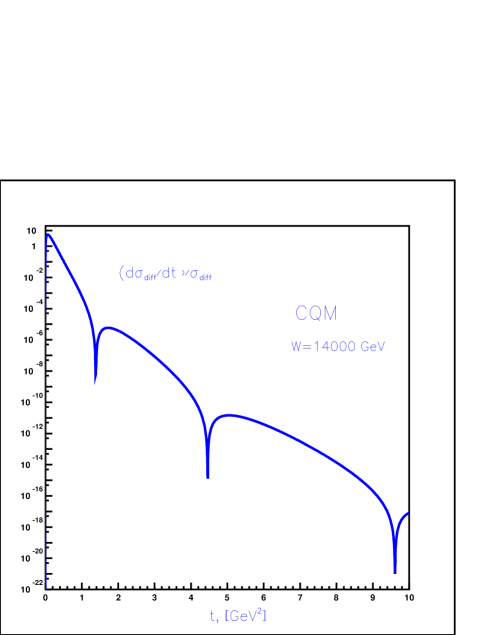
Figure 6: CQM LHC prediction for the t-dependence of the low mass diffractive differential cross section.

3.2.3 Two channel model

Our reproduction of $\sigma_{tot}$, $\sigma_{el}$, $B_{el}$ and $\sigma_{sd}$ in a two channel eikonal model have been published a while ago[7]. Note that the soft data base includes the single diffraction data. Our $\frac{\chi^{2}}{d.o.f.}$ = 1.5, which is seemingly high, reflects the poor quality of the $\sigma_{sd}$ points. Note that the b-space peripheral behaviour of the diffractive channels amplitudes is maintained in the two channel scenario. Our LHC predictions for $\sigma_{tot}$ = 103.8 mb, $\sigma_{el}$ = 24.5 mb, $B_{el}$ = 20.5 $GeV^{-2}$ and $\sigma_{sd}$ = 12.0 mb. We consider these predictions, and the consequent SP calculated values, reliable as our input diffractive rescatterings are based on an effective parametrization which includes the high mass exitations. The above numbers are significant for central Higgs diffractive production, where there is a problematic background of single diffraction which mimics the sought after Higgs signal.

3.3 Survival probabilities

Using Eq. (1.5) we calculate the energy dependence of the SP for our process in the single channel eikonal model. The result is shown in Fig. 7, which compares the exclusive central di-jet SP as calculated in the four models we have considered. For a single channel model we see that the profile function for the soft interaction does not considerably affect the value of the SP. The GP and PP profiles produce a small SP difference at the ISR energies, but at higher energies, Tevatron and above, the results are essentially the same.

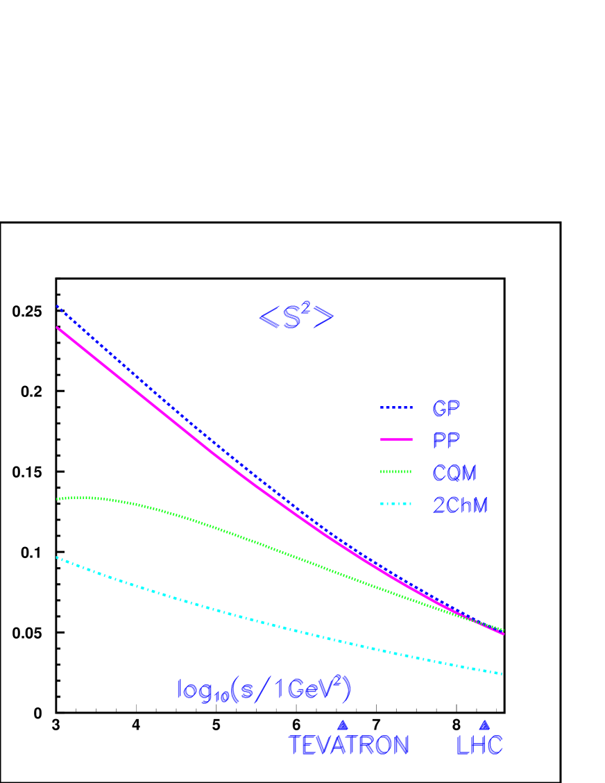
Figure 7: Energy dependence of the survival probability for exclusive central di-jet production as calculated with the four models we have considered.

In Section II.C we have explored the two component structure of $\frac{d\sigma_{H}}{d^{2}b}$, (Eq.Eq. (2.29)). Fig. 8 examines the impact of the inelastic component in the calculation of SP for our process in a single channel model with a PP profile. The results show a relatively small difference (within 10% accuracy) between a single elastic component and the sum of elastic and non elastic components (see II.C for details). An increase of the fraction of the inelastic production does not change the value of the SP significantly.

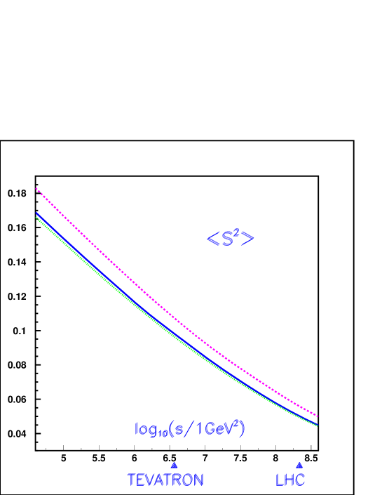
Figure 8: Energy dependence of the survival probability for di-jet production in the eikonal single channel model with a PP profile. The upper curve corresponds to the final state production of two nucleons. The lower curves take into account the inelastic production of excited states assuming either Eq. (2.29), or that at t=0 the elastic and inelastic production have the same amplitude. The two last cases can hardly be distinguished.

Fig. 7 details the SP predictions of the four models we have examined. We aim, on the basis of these predictions, to suggest upper and lower bounds for the SP corresponding to exclusive central diffractive di-jet production at the LHC. Examining Fig. 7 we observe that SP calculated in the two channel model is consistently lower than the corresponding single channel model and CQM predicted SP values. This may serve as a guide in our attempt to suggest a margin of error in the determination of SP at the LHC.

When assessing to higher SP bound, we note that the CQM SP is much lower than the single channel values at $W\,<\,1000\,GeV$, with a difference that gets smaller with increased energy. The two predictions are approximately the same, 6.0$\pm 0.1\%$, at the LHC energy and they cross just above the LHC. This suggests a 5-6$\%$ as the upper bound for the calculated SP at the LHC. We consider the SP estimates with models neglecting the diffractive channel rescatterings to over-estimate the calculated SP output. Prudency suggests, thus, an upper SP bound of 4- 5$\%$, which is moderately smaller than the predictions of the single channel models and CQM.

The two channel eikonal prediction for exclusive central diffractive di-jet production at the LHC is 2.7$\%$, compared with 3.6$\%$ for the corresponding inclusive central di-jet production[24]. The two channel input is $v\,=\,\sqrt{3}$, $B_{GG}\,=\,3.6GeV^{-2}$ and $B_{GG}^{in}\,=\,1.0GeV^{-2}$. Our two channel predicted SP at the LHC is almost identical to the KKMR[32] value. This is very supportive of a SP = 2.5-3.0$\%$ at the LHC.

It is instructive to compare our model with the KKMR model[32]. The two models are defined as ”two channels”, but are, actually, rather different.
1) Our two channel eikonal definition, for either soft or hard diffraction, consistently refers to two possible modes of soft rescattering, i.e. elastic and diffractive. Accordingly, both elastic and diffractive states in a $p-p$ scattering are presented as a linear combination of our two orthogonal base wave functions $\Psi_{1}$ and $\Psi_{2}$. In our two channel model we neglect the double diffraction channel, which is exceedingly small in the ISR-Tevatron energy range. The screening opacities of our input eikonal matrix have different b=0 normalizations, i.e. different $\nu$ values, and different b-dependences which reflect our different input for the elastic and diffractive forward differential slopes.
2) In the KKMR model for soft interactions the eikonal matrix is defined in a similar way to ours. Note, though, that their diffractive eikonal components are restricted to low diffractive mass. The screening opacities have the same b-dependence, identical to the b-dependence of the single channel elastic opacity, having a different b=0 normalizations. Unlike our input, KKMR do not neglect the double diffractive channel.
3) It is no surprise that KKMR obtain a very high LHC prediction for $\sigma_{dd}=9.5mb$, which is comparable to their predicted $\sigma_{sd}$. KKMR predict, thus, an inelastic diffractive cross section $\sigma_{sd}\,+\,\sigma_{dd}\,=\,18.9-24.9\,mb$, relative to a $\sigma_{tot}\,=\,99.1-104.5\,mb$. Our predction is $\sigma_{sd}\,=\,12.0\,mb$, which may be corrected by a small value $\sigma_{dd}$, relative to a $\sigma_{tot}\,=\,103.8\,mb$. Note that we were not successful in reproducing the KKMR fit for $\sigma_{el}$ and $B_{el}$. KKMR have not published a detailed prediction for $\sigma_{sd}$. Their quoted LHC value for single diffraction is comparable to ours.
4) In the KKMR model the hard process has two dynamical components treated as two eikonal chennels. Two sets, with two components each, were studied and have been shown to produce very similar results. In our two channel model the hard diffractive proces has two components associated with the possibility of either an elastic or inelastic diffractive initial rescattering preceeding the hard process. The SP is calculated accordingly.
5) In our model we make a weak assumption in which the ratio between the elastic and diffractive couplings is the same for soft and hard Pomerons. Consequently, we are able to associate the hard amplitude with HERA DIS experimental data resulting in eikonal opacities which are different in their b=0 normalization as well as their b-dependence. KKMR make a much stronger assumption in which all opacities, soft and hard, have the same b-dependence and a normalization which is determind by the above coupling ratio assumption.
6) Regardless of the above the actual KKMR SP results are remarkably close to ours. This result deserves a clarification in the future.

4 Transverse momentum dependence of the cross section

In the following investigation we have calculated the dependence of the output di-jet cross section on $p_{1,t}$ and $p_{2,t}$. This calculation provides the differential information on the t dependence of the cross section and SP of the process. The importance of this differential calculation is that it offers a refined method to discriminate between different models and/or parametrizations leading to compatible values of SP. We define a damping factor

$$D_{SP}\left(p_{1,t},p_{2,t}\right)\,\,=\,\,\frac{\frac{d\sigma}{d^{2}p_{1t}\,d^{2}\,p_{2t}\,dy_{1}\,dy_{2}}}{\int d^{2}p_{1t}\,d^{2}\,p_{2t},\frac{d\sigma}{d^{2}p_{1t}\,d^{2}\,p_{2t},dy_{1}\,dy_{2}}}.$$ (4.79)

In a single channel eikonal model,

$$D_{1C}\,=\,\frac{|\int\,d^{2}\,b_{1}\,d^{2}b_{2}\,e^{i\,\vec{p}_{1t}\,\cdot\,\vec{b}_{1}\,+\,i\,\vec{p}_{2t}\,\cdot\,\vec{b}_{2}}A_{H}(b_{1})\,A_{H}(b_{2})\,\,A_{S}\left((\vec{b}_{1}\,+\,\vec{b}_{2})^{2}\right)|^{2}}{\int\,d^{2}\,b_{1}\,d^{2}b_{2}\,|A_{S}\left((\vec{b}_{1}\,+\,\vec{b}_{2})^{2}\right)A_{H}(b_{1})\,A_{H}(b_{2})|^{2}}.$$ (4.80)

From its definition the value of the SP is dependent on the b-distribution of the soft amplitude profile. Should we have an experimental information on the dependence of $D_{SP}$ on $p_{1,t}$ and $p_{2,t}$, we hope to be able to invert the above procedure and obtain information on the form of the b-profile from the differential properties of the SP.

For the generalization to a two channel model we insert Eqs. 2.59 - 2.70 into the expression for the two channel SP. Using the amplitude, given by Eq. (2.59), we can carry out the integration over $d^{2}b_{1}$ analytically, obtaining a much simpler expression.

$$D_{2C}\,=\,\frac{|A|^{2}}{\int d^{2}p_{1,t}\,d^{2}p_{2,t}|A|^{2}},$$ (4.81)

where $A=A_{1}\,+\,A_{2}\,+\,A_{3}$. Defining $\vec{b}\,=\,\vec{b}_{1}\,+\,\vec{b}_{2}$ and $\vec{p}_{12}\,=\,\vec{p}_{1,t}\,-\,\vec{p}_{2,t}$, we obtain

$$A_{1}\,\, = \,\,\frac{1}{4\pi^{2}B^{2}_{el}}\,\int\,d^{2}b\,e^{-\frac{\Omega(b)}{2}}\,s(b)\,\exp\left(-\frac{b^{2}}{4B^{2}_{el}}\,-\,\frac{1}{4}B_{el}\,p^{2}_{12}\right)\,J_{0}\left(\frac{b}{2}|\vec{p}_{1,t}\,+\,\vec{p}_{2,t}|\right),$$ (4.82)

$$A_{2}\,\, = \,\,-\frac{2\alpha\,\beta}{4\pi^{2}B_{el}\,B^{2}_{inel}}\,\int\,d^{2}b\,\,e^{-\frac{\Omega(b)}{2}}\,\,s_{D}(b)\,$$

$$\cdot \exp\left(-\frac{1}{2(B_{inel}\,+\,B_{el})}\,\{b^{2}\,+\,B_{inel}\,B_{el}\,p^{2}_{12}\}\right)\,\,J_{0}\left(\frac{b}{B_{inel}\,+\,B_{el}}\,|B_{el}\,\vec{p}_{1,t}\,+\,B_{inel}\,\vec{p}_{2,t}|\right),$$

$$A_{3} = A_{2}\left(\vec{p}_{1,t}\leftrightarrow\vec{p}_{2,t}\right).$$ (4.84)

Fig. 9 and Fig. 10 show the single channel di-jet factor $D_{1C}$ with GP and PP b-profiles as a function of the transverse momenta of the produced protons in the final state. We predict a typical minima at $p_{1,t}\,\approx 1.75-2\,{\,\mbox{GeV}}$. This behaviour is a manifestation of the wave nature of our diffractive scattering process. It depends on the scale of the soft profile b-distribution. From Fig. 9 and Fig. 10 one can see that the minima $p_{t}$ position depends on both the energy of $p_{1,t}$ and $p_{2,t}$ and the angle $\theta$ between them. As stated, we hope that a future measurement of this dependence will provide valuable information which will add to our knowledge of the soft interaction amplitude in QCD. To get some initial information on the angular distribution, we have chosen (for convenience) $\theta\,=\,0,\,\pi/2,and\,\pi$.

In Fig. 11 and Fig. 12 we compare the transverse momentum distribution of the di-jet production differential cross section with the corresponding elastic cross section. These figures illustrate that the di-jet cross section has quite a different structure of minima than the elastic cross section, where the positions of these minima move to smaller values of $p_{t}$ at higher energies. Comparing with the experimental data (for data see Ref.[29] and references therein), we deduce that this data is compatible with the PP profile describing the structure of the minima and maxima in proton-proton collisions in the energy range of $W=\sqrt{s}=20-65\,GeV$. Our parametrizations for the profile function give a range of predictions for the di-jet production at the LHC. The difference between the GP and PP parametrizations, as far as $p_{t}$ dependence of the di-jet cross section is concerned, is much smaller than for the elastic cross section.

A most interesting result is the striking difference between the t-dependence of the damping factors, defined in Eq. (4.79), obtained in the single and two channel eikonal models. This difference is clearly seen in Fig. 13 in which GP profiles were used. The single channel model leads to a dip and to a slope at $p_{1,t}$=0 which is equal to $B_{GP}$ without a suppression due to SP. In the two channel eikonal model we do not have any dip at $p_{1,t}\,\leq 2\,\,GeV$ and the slope turns out to be much smaller than the slope obtained from the single channel eikonal model.

This result can be anticipated from the general formula of Eq. (2.56) and Eq. (2.58) which show that the damping factor is proportional to a contribution of the order of $\beta$ while the elastic cross section is proportional to $\beta^{2}$ (see Ref.[7]).

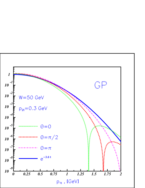
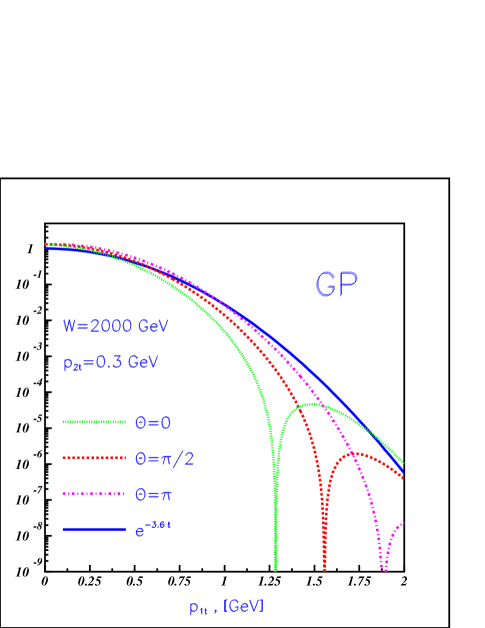
Fig. 9-a	Fig. 9-b
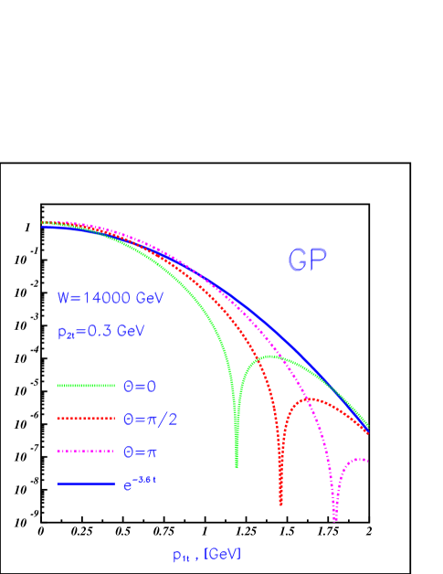
Fig. 9-c

Figure 9: Transverse momentum dependence of the cross section factor $D$ in a single channel model with a Gaussian b-profile (GP) for various $\theta$ values. We also show an $\exp(-3.6|t|)$ dependence corresponding to to the hard slope $B_{GG}$.

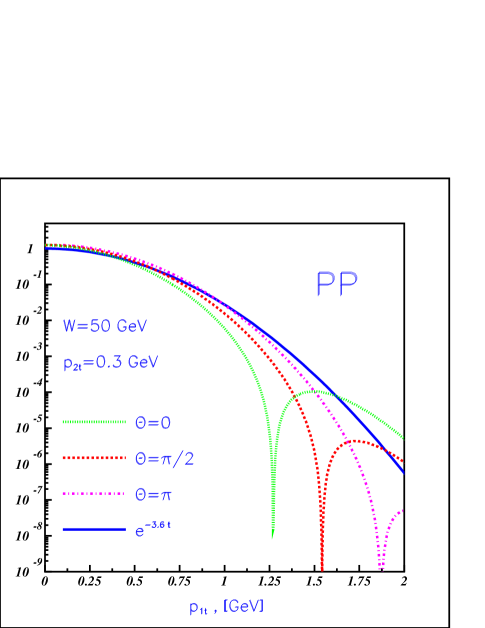
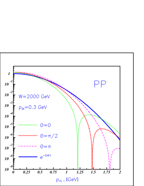
Fig. 10-a	Fig. 10-b
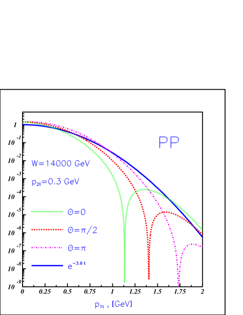
Fig. 10-c

Figure 10: Transverse momentum dependence of the cross section factor $D$ in a single channel model with a power like b-profile (PP) for various $\theta$ values. We also show an $\exp(-3.6|t|)$ dependence corresponding to to the hard slope $B_{GG}$.

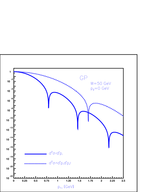
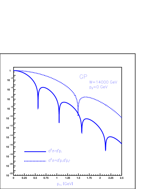
Fig. 11-a	Fig. 11-b

Figure 11: Transverse momentum dependence of the cross section factor $D$ in a single channel model with a Gaussian b-profile (GP) compared with the corresponding elastic cross section.

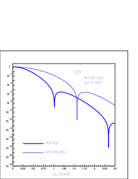
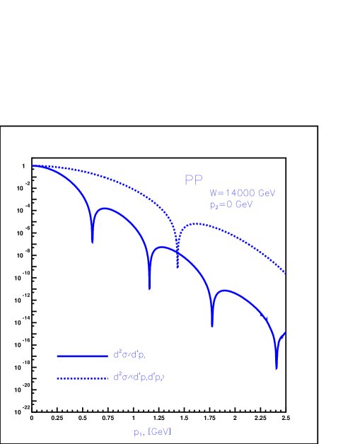
Fig. 12-a	Fig. 12-b

Figure 12: Transverse momentum dependence of the cross section factor $D$ in a single channel model with a power like b-profile (PP) compared with the corresponding elastic cross section.

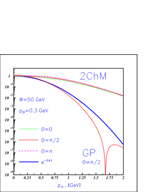
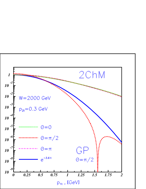
Fig. 13-a	Fig. 13-b
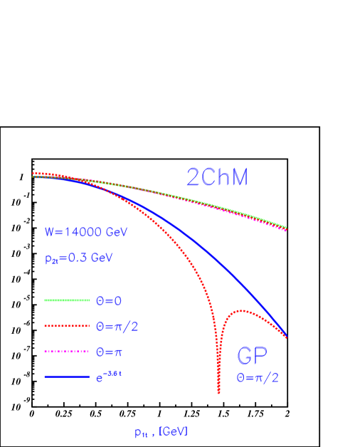
Fig. 13-c

Figure 13: Transverse momentum dependence of the cross section factor $D$ in a two channel model with Gaussian b-profiles (GP) for various $\Theta$ values, compared with the corresponding single channel elastic cross section with $\theta=\pi/2$. We also show an $\exp(-3.6|t|)$ dependence corresponding to to the two channel input hard slope $B_{GG}$.

5 Conclusions

In this paper we have calculated the large rapidity gap survival probability $<|S|^{2}>$, for exclusive central dijet production at the LHC. Our assessments are of particular interest as the SP we have calculated correspond also to a central exclusive diffractive production of Higgs. The unique feature of our treatment is that we explicitly included the impact parameter dependence of the hard amplitude in our evaluation of SP. This b-dependence appears in the proton-hard Pomeron vertex, whose structure was deduced from information obtained from the DIS production of $J/\psi$.

The calculation of the LRG SP requires knowledge of both the hard and soft components of the hadron-hadron interactions. As there is no reliable theory for the soft component, we employed four phenomenological eikonal models to describe the soft processes. These models are:
1) A single channel model with an exponential dependence in t for the proton-soft Pomeron vertex.
2) A single channel model with a power-like behaviour for the proton-soft Pomeron vertex.
3) The CQM, which is a non Regge two component soft model, where we have assumed that this vertex is given by the proton electromagnetic form factor approximated by a dipole.
For cases 2) and 3), we have to integrate over b numerically, while for case 1), we have an analytical expression.
4) To these we add the two channel model whose main advantage is that it is the only model considered that properly reproduces the available diffractive data.

All four models considered were utilized to calculate the SP of an exclusive central hard di-jet production. The two channel model predicts for this SP a value of 0.027, which is almost identical to the KKMR prediction. These should be compared with a 0.036 value for the equivalent inclusive calculation[24]. The other three models have compatible prediction of 0.06. We consider this value to be some what over estimated as these models neglect the diffractive rescattering which increases the eikonal overall screening and, thus, reduces the SP. We prudently conclude that the LHC SP we have studied lies between 0.03 - 0.05.

The single channel cross-section for the dijet production as a function of $p_{t}$, has a typical structure of minima at certain values of $p_{t}$, which is dependent both on the angle between $p_{t1}$ and $p_{t2}$ of the two jets, and on their energy. Positions of the minima are model dependent.

The most interesting result of this paper is the fact that the two channel model predicts quite different dependence of the damping factor versus the transverse momenta. The central prediction is that there are no dips for $p_{t}\,\leq\,2\,GeV$. Also, the slope at $p_{t}=0$ turns out to be much smaller than for the one channel eikonal model. Both features stem from the general properties of the two channel model and we firmly believe that this prediction should assist to select the appropriate models for the description of SP directly from the experimental data. Since the general behaviour of the damping factor depends weakly on energy we suggest assessing the damping factor at the Tevatron energies. We would like to stress that the calculation of the damping factor show such simplicity and elegance that we believe they have a deeper meaning than being just a consequence of a particular model.

References

-
[1]
Yu. L. Dokshitzer, V. Khoze and S.I. Troyan, Proc.“Physics in
Collisions 6”, p. 417, ed. M. Derrick, WS 1987; Sov. J. Nucl.
Phys. 46, 712 (1987).
Y. L. Dokshitzer, V. A. Khoze and T. Sjostrand, Phys. Lett. B274, 116 (1992). - [2] J. D. Bjorken, Int. J. Mod. Phys. A7, 4189 (1992); Phys. Rev. D47, 101 (1993).
- [3] E. Gotsman, E.M. Levin and U. Maor, Phys. Rev. D49, R4321 (1994).
- [4] H. Chehime and D. Zeppenfeld, Phys. Rev. D47, 3898 (1993).
- [5] R. S. Fletcher and T. Stelzer, Phys. Rev. D48, 5162 (1993).
- [6] E. Gotsman, E. Levin and U. Maor, Phys. Lett. B309 (1993) 199 (1993); Phys. Lett. B438 229 (1998).
- [7] E. Gotsman, E. Levin and U. Maor, Phys. Rev. D60 094011 (1999); Phys. Lett. B452, 387 (1999).
- [8] V. A. Khoze, A. D. Martin and M. G. Ryskin, Eur. Phys. J. C24 581 (2002), Eur. Phys. J. C21 521 (2001), Eur. Phys. J. C14 525 (2000).
- [9] A. B. Kaidalov, V. A. Khoze, A. D. Martin and M. G. Ryskin, Eur. Phys. J. C21 521 (2001).
- [10] M. M. Block and F. Halzen, Phys. Rev. D63, 114004 (2001).
- [11] For recent reviews see: K. Goulianos, Proceedings of Diffraction 2002, Alushta (Crimea), Kluwer Academic Pub. (2002) 13; J. Phys. G26 (2000) 716; Nucl. Phys. Proc. Suppl. 99A (2001) 37; hep-ph/0407035.
-
[12]
ZEUS Collaboration,
Eur. Phys. J. C6 43 (1999);
Phys. Rev. Lett. 84 5083 (2000).
H1 Collaboration, Nucl. Phys. B429 477 (1994); Phys. Lett. B348 681 (1995); Zeit. Phys. C76 613 (1997). -
[13]
F. Low, Phys. Rev. D12, 163 (1975).
S. Nussinov, Phys. Rev. Lett. 34, 1286 (1975); Phys. Rev. D14, 244 (1976). - [14] D. Kharzeev and E. Levin, Nucl. Phys. B578 351 (2000).
- [15] D. E. Kharzeev, Y. V. Kovchegov and E. Levin, Nucl. Phys. A690 621 (2001).
-
[16]
E. V. Shuryak and I. Zahed,
Phys. Rev. D67 YV054025 (2003).
M. A. Nowak, E. V. Shuryak and I. Zahed, Phys. Rev. D64 034008 (2001) -
[17]
R. A. Janik,
Acta Phys. Polon. B33 3615 (2002);
Phys. Lett. B500 118 (2001).
R. A. Janik and R. Peschanski, Nucl. Phys. B586, 163 (2000); Nucl. Phys. B625, 279 (2002). - [18] O. Nachtmann, Annals Phys. 209, 436 (1991).
- [19] F. Schrempp and A. Utermann, Phys. Lett. B543 197 (2002).
- [20] D. Kharzeev, E. Levin and K. Tuchin, Phys. Lett. B547 21 (2002).
- [21] E. Ferreiro, E. Iancu, K. Itakura and L. McLerran, Nucl. Phys. A710 373 (2002).
- [22] A. Donnachie and P.V. Landshoff, Nucl. Phys. B244, 322 (1984); Nucl. Phys. B267, 690 (1986); Phys. Lett. B296, 227 (1992); Z. Phys. C61, 139 (1994).
- [23] H. Kowalski and D. Teaney, Phys. Rev. D68 114005 (2003).
- [24] E. Gotsman, E. Levin, U. Maor, E. Naftali and A. Prygarin, Proceedings of HERA and LHC Workshop, CERN Pub. (2005).
-
[25]
E. A. Kuraev, L. N. Lipatov, and F. S. Fadin,
Sov. Phys. JETP 45 199 (1977).
Ya. Ya. Balitsky and L. N. Lipatov, Sov. J. Nucl. Phys. 28 22 (1978). -
[26]
V. N. Gribov and L. N. Lipatov,
Sov. J. Nucl. Phys. 15 438 (1972).
G. Altarelli and G. Parisi, Nucl. Phys. B126 298 (1977).
Yu. l. Dokshitser, Sov. Phys. JETP 46 641 (1977). - [27] V. A. Khoze, A. D. Martin and M. G. Ryskin, Eur. Phys. J. C19 477 (2001) [Erratum-ibid. C20 599 (2001)]; Phys. Rev. D56 5867 (1997).
- [28] “ Regge theory of low- hadtronic interaction”, ed. Luca Caneschi, 1989,North Holland Pub.
- [29] V. Barone and E. Predazzi, “ High-Energy Particle Diffraction”, Springer Verlag Pub. (2002).
- [30] S. Bondarenko and E. Levin, “Proton proton interaction in constituent quarks model at LHC energies,” arXiv:hep-ph/0511124.
- [31] E. Gotsman, E. Levin, H. Kowalski, U. Maor, and A. Prygarin, arXiv:hep-ph/0512254 (version 1).
- [32] V. A. Khoze, A. D. Martin and M. G. Ryskin, Eur. Phys. J. C18 167 (2000).
- [33] Particle Data Group, “Review of Particle Physics” Eur. Phys. J. C3 (1998) 1, and references therein.