Highlights of the B-Physics Landscape

Abstract

The exploration of the quark-flavour sector of the Standard Model is one of the hot topics in particle physics of this decade. In these studies, which show a fruitful interplay between theory and experiment, the $B$-meson system offers a particularly interesting laboratory. After giving an introduction to quark-flavour mixing and CP violation as well as to the theoretical tools to deal with non-leptonic $B$ decays, we discuss popular avenues for new physics to enter the roadmap of quark-flavour physics. This allows us to have a detailed look at the $B$-factory benchmark modes $B^{0}_{d}\to J/\psi K_{\rm S}$, $B^{0}_{d}\to\phi K_{\rm S}$ and $B^{0}_{d}\to\pi^{+}\pi^{-}$, with a particular emphasis of the impact of new physics. We then perform an analysis of the $B\to\pi K$ puzzle, which may indicate new sources of CP violation in the electroweak penguin sector, and discuss its implications for rare $B$ and $K$ decays. The next topic is given by $b\to d$ penguin processes, which are now starting to become accessible at the $B$ factories, thereby representing a new territory of the $B$-physics landscape. Finally, we discuss the prospects for $B$-decay studies at the Large Hadron Collider, where the $B^{0}_{s}$-meson system plays an outstanding rôle.

1 Introduction

The history of CP violation, i.e. the non-invariance of the weak interactions with respect to a combined charge-conjugation (C) and parity (P) transformation, goes back to the year 1964, where this phenomenon was discovered through the observation of $K_{\rm L}\to\pi^{+}\pi^{-}$ decays [1], which exhibit a branching ratio at the $10^{-3}$ level. This surprising effect is a manifestation of indirect CP violation, which arises from the fact that the mass eigenstates $K_{\rm L,S}$ of the neutral kaon system, which shows $K^{0}$–$\bar{K}^{0}$ mixing, are not eigenstates of the CP operator. In particular, the $K_{\rm L}$ state is governed by the CP-odd eigenstate, but has also a tiny admixture of the CP-even eigenstate, which may decay through CP-conserving interactions into the $\pi^{+}\pi^{-}$ final state. These CP-violating effects are described by the following observable:

$$\varepsilon_{K}=(2.280\pm 0.013)\times 10^{-3}\times e^{i\pi/4}.$$ (1)

On the other hand, CP-violating effects may also arise directly at the decay-amplitude level, thereby yielding direct CP violation. This phenomenon, which leads to a non-vanishing value of a quantity Re$(\varepsilon_{K}^{\prime}/\varepsilon_{K})$, could eventually be established in 1999 through the NA48 (CERN) and KTeV (FNAL) collaborations [2]; the final results of the corresponding measurements are given by

$$\mbox{Re}(\varepsilon_{K}^{\prime}/\varepsilon_{K})=\left\{\begin{array}[]{ll}(14.7\pm 2.2)\times 10^{-4}&\mbox{(NA48 \cite[cite]{[\@@bibref{}{NA48-final}{}{}]})}\\ (20.7\pm 2.8)\times 10^{-4}&\mbox{(KTeV \cite[cite]{[\@@bibref{}{KTeV-final}{}{}]}).}\end{array}\right.$$ (2)

In this decade, there are huge experimental efforts to further explore CP violation and the quark-flavour sector of the Standard Model (SM). In these studies, the main actor is the $B$-meson system, where we distinguish between charged and neutral $B$ mesons, which are characterized by the following valence-quark contents:

$$B^{+}\sim u\bar{b},\quad B^{+}_{c}\sim c\bar{b},\quad B^{0}_{d}\sim d\bar{b},\quad B^{0}_{s}\sim s\bar{b}.$$ (3)

The asymmetric $e^{+}e^{-}$ $B$ factories at SLAC and KEK with their detectors BaBar and Belle, respectively, can only produce $B^{+}$ and $B^{0}_{d}$ mesons (and their anti-particles) since they operate at the $\Upsilon(4S)$ resonance, and have already collected ${\cal O}(10^{8})$ $B\bar{B}$ pairs of this kind. Moreover, first $B$-physics results from run II of the Tevatron were reported from the CDF and D0 collaborations, including also $B^{+}_{c}$ and $B^{0}_{s}$ studies, and second-generation $B$-decay studies will become possible at the Large Hadron Collider (LHC) at CERN, in particular thanks to the LHCb experiment, starting in the autumn of 2007. For the more distant future, an $e^{+}$–$e^{-}$ “super-$B$ factory” is under consideration, with an increase of luminosity by up to two orders of magnitude with respect to the currently operating machines. Moreover, there are plans to measure the very “rare” kaon decays $K^{+}\to\pi^{+}\nu\bar{\nu}$ and $K_{\rm L}\to\pi^{0}\nu\bar{\nu}$, which are absent at the tree level within the SM, at CERN and KEK/J-PARC.

In 2001, CP-violating effects were discovered in the $B$-meson system with the help of $B_{d}\to J/\psi K_{\rm S}$ decays by the BaBar and Belle collaborations [5], representing the first observation of CP violation outside the kaon system. This particular kind of CP violation originates from the interference between $B^{0}_{d}$–$\bar{B}^{0}_{d}$ mixing and $B^{0}_{d}\to J/\psi K_{\rm S}$, $\bar{B}^{0}_{d}\to J/\psi K_{\rm S}$ decay processes, and is referred to as “mixing-induced” CP violation. In the summer of 2004, also direct CP violation could be detected in $B_{d}\to\pi^{\mp}K^{\pm}$ decays [6], thereby complementing the measurement of a non-zero value of $\mbox{Re}(\varepsilon_{K}^{\prime}/\varepsilon_{K})$.

Studies of CP violation and flavour physics are particularly interesting since “new physics” (NP), i.e. physics lying beyond the SM, typically leads to new sources of flavour and CP violation. Furthermore, the origin of the fermion masses, flavour mixing, CP violation etc. lies completely in the dark and is expected to involve NP, too. Interestingly, CP violation offers also a link to cosmology. One of the key features of our Universe is the cosmological baryon asymmetry of ${\cal O}(10^{-10})$. As was pointed out by Sakharov [7], the necessary conditions for the generation of such an asymmetry include also the requirement that elementary interactions violate CP (and C). Model calculations of the baryon asymmetry indicate, however, that the CP violation present in the SM seems to be too small to generate the observed asymmetry [8]. On the one hand, the required new sources of CP violation could be associated with very high energy scales, as in “leptogenesis”, where new CP-violating effects appear in decays of heavy Majorana neutrinos [9]. On the other hand, new sources of CP violation could also be accessible in the laboratory, as they arise naturally when going beyond the SM.

Before searching for NP, it is essential to understand first the picture of flavour physics and CP violation arising in the framework of the SM, where the Cabibbo–Kobayashi–Maskawa (CKM) matrix – the quark-mixing matrix – plays the key rôle [10, 11]. The corresponding phenomenology is extremely rich [12]. In general, the key problem for the theoretical interpretation is related to strong interactions, i.e. to “hadronic” uncertainties. A famous example is $\mbox{Re}(\varepsilon_{K}^{\prime}/\varepsilon_{K})$, where we have to deal with a subtle interplay between different contributions which largely cancel [13]. Although the non-vanishing value of this quantity has unambiguously ruled out “superweak” models of CP violation [14], it does currently not allow a stringent test of the SM.

In the $B$-meson system, there are various strategies to eliminate the hadronic uncertainties in the exploration of CP violation (simply speaking, there are many $B$ decays). Moreover, we may also search for relations and/or correlations that hold in the SM but could well be spoiled by NP. These topics will be the focus of this review. The outline is as follows: in Section 2, we discuss the quark mixing in the SM by having a closer look at the CKM matrix and the associated unitarity triangles. The main actor of this review – the $B$-meson system – will then be introduced in Section 3. There we turn to the formalism of $B^{0}_{q}$–$\bar{B}^{0}_{q}$ mixing ($q\in\{d,s\}$), give an introduction to non-leptonic $B$ decays, which play the key rôle for CP violation, and discuss popular avenues for NP to enter the strategies to explore this phenomenon. In Section 4, we then apply these considerations to the $B$-factory benchmark modes $B^{0}_{d}\to J/\psi K_{\rm S}$, $B^{0}_{d}\to\phi K_{\rm S}$ and $B^{0}_{d}\to\pi^{+}\pi^{-}$, and address the possible impact of NP. Since the data for certain $B\to\pi K$ decays show a puzzling pattern for several years, we have devoted Section 5 to a detailed discussion of this “$B\to\pi K$ puzzle” and its interplay with rare $K$ and $B$ decays. In Section 6, we focus on $b\to d$ penguin processes, which are now coming within experimental reach at the $B$ factories, thereby offering an exciting new playground. Finally, in Section 7, we discuss $B$-decay studies at the LHC, where the physics potential of the $B^{0}_{s}$-meson system can be fully exploited. The conclusions and a brief outlook are given in Section 8.

For textbooks dealing with CP violation, the reader is referred to Refs. [15]–[17], while a selection of alternative recent reviews can be found in Refs. [18]–[21].

2 Quark Mixing in the Standard Model

2.1 The CKM Matrix

In the SM, CP-violating phenomena may originate from the charged-current interaction processes of the quarks, $D\to UW^{-}$, where $D\in\{d,s,b\}$ and $U\in\{u,c,t\}$ denote the down- and up-type quark flavours, respectively, and the $W^{-}$ is the usual $SU(2)_{\rm L}$ gauge boson. The generic “coupling strengths” $V_{UD}$ of these processes are the elements of a $3\times 3$ matrix, the CKM matrix [10, 11]. It connects the electroweak states $(d^{\prime},s^{\prime},b^{\prime})$ of the down, strange and bottom quarks with their mass eigenstates $(d,s,b)$ through the following unitary transformation:

$$\left(\begin{array}[]{c}d^{\prime}\\ s^{\prime}\\ b^{\prime}\end{array}\right)=\left(\begin{array}[]{ccc}V_{ud}&V_{us}&V_{ub}\\ V_{cd}&V_{cs}&V_{cb}\\ V_{td}&V_{ts}&V_{tb}\end{array}\right)\cdot\left(\begin{array}[]{c}d\\ s\\ b\end{array}\right)\equiv\hat{V}_{\rm CKM}\cdot\left(\begin{array}[]{c}d\\ s\\ b\end{array}\right),$$ (4)

and is, therefore, a unitary matrix. Since this feature ensures the absence of flavour-changing neutral-current (FCNC) processes at the tree level in the SM, it is at the basis of the Glashow–Iliopoulos–Maiani (GIM) mechanism [22]. Expressing the non-leptonic charged-current interaction Lagrangian in terms of the mass eigenstates (4), we obtain

$${\cal L}_{\mbox{{\scriptsize int}}}^{\mbox{{\scriptsize CC}}}=-\frac{g_{2}}{\sqrt{2}}\left(\begin{array}[]{ccc}\bar{u}_{\mbox{{\scriptsize L}}},&\bar{c}_{\mbox{{\scriptsize L}}},&\bar{t}_{\mbox{{\scriptsize L}}}\end{array}\right)\gamma^{\mu}\,\hat{V}_{\mbox{{\scriptsize CKM}}}\left(\begin{array}[]{c}d_{\mbox{{\scriptsize L}}}\\ s_{\mbox{{\scriptsize L}}}\\ b_{\mbox{{\scriptsize L}}}\end{array}\right)W_{\mu}^{\dagger}\,\,+\,\,\mbox{h.c.,}$$ (5)

where $g_{2}$ is the $SU(2)_{\mbox{{\scriptsize L}}}$ gauge coupling, and $W_{\mu}^{(\dagger)}$ the field of the charged $W$ bosons.

Since the CKM matrix elements governing a $D\to UW^{-}$ transition and its CP conjugate $\bar{D}\to\bar{U}W^{+}$ are related to each other through

$$V_{UD}\stackrel{{\scriptstyle{CP}}}{{\longrightarrow}}V_{UD}^{\ast},$$ (6)

we observe that CP violation is associated with complex phases of the CKM matrix.

2.2 The Phase Structure of the CKM Matrix

We have the freedom of redefining the up- and down-type quark fields as follows:

$$U\to\exp(i\xi_{U})U,\quad D\to\exp(i\xi_{D})D.$$ (7)

Performing such transformations in (5), the invariance of the charged-current interaction Lagrangian implies the following transformations of the CKM matrix elements:

$$V_{UD}\to\exp(i\xi_{U})V_{UD}\exp(-i\xi_{D}).$$ (8)

If we consider a general $N\times N$ quark-mixing matrix, where $N$ denotes the number of fermion generations, and eliminate unphysical phases through these transformations, we are left with the following quantities to parametrize the quark-mixing matrix:

$$\underbrace{\frac{1}{2}N(N-1)}_{\mbox{Euler angles}}\,+\,\underbrace{\frac{1}{2}(N-1)(N-2)}_{\mbox{complex phases}}=(N-1)^{2}.$$ (9)

Applying this expression to $N=2$ generations, we observe that only one rotation angle – the Cabibbo angle $\theta_{\rm C}$ [10] – is required for the parametrization of the $2\times 2$ quark-mixing matrix, which can be written as

$$\hat{V}_{\rm C}=\left(\begin{array}[]{cc}\cos\theta_{\rm C}&\sin\theta_{\rm C}\\ -\sin\theta_{\rm C}&\cos\theta_{\rm C}\end{array}\right),$$ (10)

where the value of $\sin\theta_{\rm C}=0.22$ follows from the experimental data for $K\to\pi\ell\bar{\nu}_{\ell}$ decays. On the other hand, in the case of $N=3$ generations, the parametrization of the corresponding $3\times 3$ quark-mixing matrix involves three Euler-type angles and a single complex phase. This complex phase allows us to accommodate CP violation in the SM, as was pointed out by Kobayashi and Maskawa in 1973 [11]. The corresponding picture is referred to as the Kobayashi–Maskawa (KM) mechanism of CP violation.

The Particle Data Group advocates the following “standard parametrization” [23]:

$$\hat{V}_{\rm CKM}=\left(\begin{array}[]{ccc}c_{12}c_{13}&s_{12}c_{13}&s_{13}e^{-i\delta_{13}}\\ -s_{12}c_{23}-c_{12}s_{23}s_{13}e^{i\delta_{13}}&c_{12}c_{23}-s_{12}s_{23}s_{13}e^{i\delta_{13}}&s_{23}c_{13}\\ s_{12}s_{23}-c_{12}c_{23}s_{13}e^{i\delta_{13}}&-c_{12}s_{23}-s_{12}c_{23}s_{13}e^{i\delta_{13}}&c_{23}c_{13}\end{array}\right),$$ (11)

with $c_{ij}\equiv\cos\theta_{ij}$ and $s_{ij}\equiv\sin\theta_{ij}$. If we redefine the quark-field phases appropriately, $\theta_{12}$, $\theta_{23}$ and $\theta_{13}$ can all be made to lie in the first quadrant. The advantage of this parametrization is that the mixing between two generations $i$ and $j$ vanishes if $\theta_{ij}$ is set to zero. In particular, for $\theta_{23}=\theta_{13}=0$, the third generation decouples, and the submatrix describing the mixing between the first and second generations takes the same form as (10).

2.3 The Wolfenstein Parametrization

The experimental data for the charged-current interactions of the quarks exhibit an interesting hierarchy [23]: transitions within the same generation involve CKM matrix elements of ${\cal O}(1)$, those between the first and the second generation are associated with CKM elements of ${\cal O}(10^{-1})$, those between the second and the third generation are related to CKM elements of ${\cal O}(10^{-2})$, and those between the first and third generation are described by CKM matrix elements of ${\cal O}(10^{-3})$. It would be useful for phenomenological applications to have a parametrization of the CKM matrix available that makes this pattern explicit [24]. To this end, we introduce a set of new parameters, $\lambda$, $A$, $\rho$ and $\eta$, by imposing the following relations [25]:

$$s_{12}\equiv\lambda=0.22,\quad s_{23}\equiv A\lambda^{2},\quad s_{13}e^{-i\delta_{13}}\equiv A\lambda^{3}(\rho-i\eta).$$ (12)

If we go back to the standard parametrization (11), we obtain an exact parametrization of the CKM matrix in terms of $\lambda$ (and $A$, $\rho$, $\eta$), which allows us to expand each CKM element in powers of the small parameter $\lambda$. Neglecting terms of ${\cal O}(\lambda^{4})$ yields the famous “Wolfenstein parametrization” [24]:

$$\hat{V}_{\mbox{{\scriptsize CKM}}}=\left(\begin{array}[]{ccc}1-\frac{1}{2}\lambda^{2}&\lambda&A\lambda^{3}(\rho-i\eta)\\ -\lambda&1-\frac{1}{2}\lambda^{2}&A\lambda^{2}\\ A\lambda^{3}(1-\rho-i\eta)&-A\lambda^{2}&1\end{array}\right)+{\cal O}(\lambda^{4}).$$ (13)

On the other hand, also higher-order terms of the expansion in $\lambda$ can straightforwardly be included by following the recipe described above.

(a) (b)          

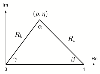
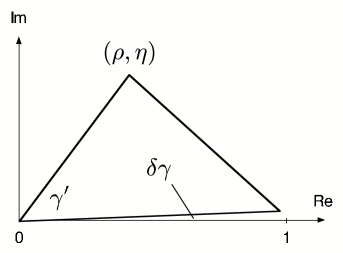
Figure 1: The two non-squashed unitarity triangles of the CKM matrix: (a) and (b) correspond to the orthogonality relations (15) and (16), respectively. In Asia, the notation $\phi_{1}\equiv\beta$, $\phi_{2}\equiv\alpha$ and $\phi_{3}\equiv\gamma$ is used for the angles of the triangle shown in (a).

2.4 The Unitarity Triangles of the CKM Matrix

Since the CKM matrix is a unitary matrix, it satisfies

$$\hat{V}_{\mbox{{\scriptsize CKM}}}^{\,\,\dagger}\cdot\hat{V}_{\mbox{{\scriptsize CKM}}}=\hat{1}=\hat{V}_{\mbox{{\scriptsize CKM}}}\cdot\hat{V}_{\mbox{{\scriptsize CKM}}}^{\,\,\dagger},$$ (14)

leading to a set of 12 equations, which consist of 6 normalization and 6 orthogonality relations. The latter can be represented as 6 triangles in the complex plane, which have all the same area. The Wolfenstein parametrization of the CKM matrix allows us straightforwardly to explore the generic shape of these triangles: we find two triangles, where one side is suppressed with respect to the others by a factor of ${\cal O}(\lambda^{2})$, and another set of two triangles, where one side is even suppressed with respect to the others by a factor of ${\cal O}(\lambda^{4})$; however, there are also two triangles, where all three sides are of the same order of magnitude. They are described by the following orthogonality relations:

$$V_{ud}V_{ub}^{\ast}+V_{cd}V_{cb}^{\ast}+V_{td}V_{tb}^{\ast} = 0$$ (15)

$$V_{ud}^{\ast}V_{td}+V_{us}^{\ast}V_{ts}+V_{ub}^{\ast}V_{tb} = 0.$$ (16)

If we keep just the leading, non-vanishing terms of the expansion in $\lambda$, these relations give actually the same result, which is given by

$$\left[(\rho+i\eta)+(1-\rho-i\eta)+(-1)\right]A\lambda^{3}=0,$$ (17)

and describes the unitarity triangle of the CKM matrix.

Following the procedure described in Subsection 2.3, we may also include the next-to-leading order corrections in the $\lambda$ expansion [25]. The degeneracy between the leading-order triangles corresponding to (15) and (16) is then lifted, and we arrive at the situation illustrated in Fig. 1. The triangle sketched in Fig. 1 (a) is a straightforward generalization of the leading-order case. Its apex takes the following coordinates [25]:

$$\bar{\rho}\equiv\rho\left(1-\frac{1}{2}\lambda^{2}\right),\quad\bar{\eta}\equiv\eta\left(1-\frac{1}{2}\lambda^{2}\right),$$ (18)

which correspond to the triangle sides

$$R_{b}=\left(1-\frac{\lambda^{2}}{2}\right)\frac{1}{\lambda}\left|\frac{V_{ub}}{V_{cb}}\right|,\quad R_{t}=\frac{1}{\lambda}\left|\frac{V_{td}}{V_{cb}}\right|.$$ (19)

This triangle is usually the one considered in the literature, and whenever referring to a unitarity triangle (UT) in the following discussion, also we shall always mean this triangle. The characteristic feature of the second triangle shown in Fig. 1 (b) is the small angle between the basis of the triangle and the real axis, satisfying

$$\delta\gamma\equiv\gamma-\gamma^{\prime}=\lambda^{2}\eta={\cal O}(1^{\circ}).$$ (20)

As we will see below, this triangle is of particular interest for the LHCb experiment.

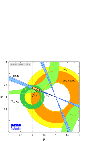
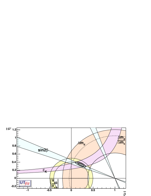
Figure 2: The most recent analyses of the CKMfitter and UTfit collaborations [26, 27].

2.5 The Determination of the Unitarity Triangle

The next obvious question is how to determine the UT. There are two conceptually different avenues that we may follow to this end:

• In the “CKM fits”, theory is used to convert experimental data into contours in the $\bar{\rho}$–$\bar{\eta}$ plane. In particular, semi-leptonic $b\to u\ell\bar{\nu}_{\ell}$, $c\ell\bar{\nu}_{\ell}$ decays and $B^{0}_{q}$–$\bar{B}^{0}_{q}$ mixing ($q\in\{d,s\}$) allow us to determine the UT sides $R_{b}$ and $R_{t}$, respectively, i.e. to fix two circles in the $\bar{\rho}$–$\bar{\eta}$ plane. Furthermore, the indirect CP violation in the neutral kaon system described by $\varepsilon_{K}$ can be transformed into a hyperbola.

• Theoretical considerations allow us to convert measurements of CP-violating effects in $B$-meson decays into direct information on the UT angles. The most prominent example is the determination of $\sin 2\beta$ through CP violation in $B^{0}_{d}\to J/\psi K_{\rm S}$ decays, but several other strategies were proposed.

The goal is to “overconstrain” the UT as much as possible. In the future, additional contours can be fixed in the $\bar{\rho}$–$\bar{\eta}$ plane through the measurement of rare decays.

In Fig. 2, we show the most recent results of the comprehensive analyses of the UT that were performed by the “CKM Fitter Group” [26] and the “UTfit collaboration” [27]. In these figures, we can nicely see the circles that are determined through the semi-leptonic $B$ decays and the $\varepsilon_{K}$ hyperbolas. Moreover, also the straight lines following from the direct measurement of $\sin 2\beta$ with the help of $B^{0}_{d}\to J/\psi K_{\rm S}$ modes are shown. We observe that the global consistency is very good. However, looking closer, we also see that the most recent average for $(\sin 2\beta)_{\psi K_{\rm S}}$ is now on the lower side, so that the situation in the $\bar{\rho}$–$\bar{\eta}$ plane is no longer “perfect”. Moreover, as we shall discuss in detail in the course of this review, there are certain puzzles in the $B$-factory data, and several important aspects could not yet be addressed experimentally and are hence still essentially unexplored. Consequently, we may hope that flavour studies will eventually establish deviations from the SM description of CP violation. Since $B$ mesons play a key rôle in these explorations, let us next have a closer look at them.

3 The Main Actor: The $B$-Meson System

3.1 A Closer Look at $B_{q}^{0}$–$\bar{B}_{q}^{0}$ Mixing

In contrast to their charged counterparts, the neutral $B_{q}$ ($q\in\{d,s\}$) mesons show $B_{q}^{0}$–$\bar{B}_{q}^{0}$ mixing, which we encountered already in the determination of the UT discussed in Subsection 2.5. This phenomenon is the counterpart of $K^{0}$–$\bar{K}^{0}$ mixing, and originates, in the SM, from box diagrams, as illustrated in Fig. 3. Thanks to $B_{q}^{0}$–$\bar{B}_{q}^{0}$ mixing, an initially, i.e. at time $t=0$, present $B^{0}_{q}$-meson state evolves into a time-dependent linear combination of $B^{0}_{q}$ and $\bar{B}^{0}_{q}$ states:

$$|B_{q}(t)\rangle=a(t)|B^{0}_{q}\rangle+b(t)|\bar{B}^{0}_{q}\rangle,$$ (21)

where $a(t)$ and $b(t)$ are governed by a Schrödinger equation of the following form:

$$i\,\frac{{\rm d}}{{\rm d}t}\left(\begin{array}[]{c}a(t)\\ b(t)\end{array}\right)=\Biggl{[}\underbrace{\left(\begin{array}[]{cc}M_{0}^{(q)}&M_{12}^{(q)}\\ M_{12}^{(q)\ast}&M_{0}^{(q)}\end{array}\right)}_{\mbox{mass matrix}}-\frac{i}{2}\underbrace{\left(\begin{array}[]{cc}\Gamma_{0}^{(q)}&\Gamma_{12}^{(q)}\\ \Gamma_{12}^{(q)\ast}&\Gamma_{0}^{(q)}\end{array}\right)}_{\mbox{decay matrix}}\Biggr{]}\cdot\left(\begin{array}[]{c}a(t)\\ b(t)\end{array}\right).$$

The special form $H_{11}=H_{22}$ of the Hamiltonian $H$ is an implication of the CPT theorem, i.e. of the invariance under combined CP and time-reversal (T) transformations.

     

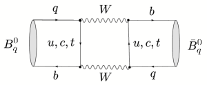
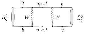
Figure 3: Box diagrams contributing to $B^{0}_{q}$–$\bar{B}^{0}_{q}$ mixing in the SM ($q\in\{d,s\}$).

In the SM, the mass and decay matrices can be calculated through the dispersive and absorptive parts of the box diagrams in Fig. 3, respectively, where the former is dominated by top-quark exchanges. Following these lines, we arrive at

$$\frac{\Gamma_{12}^{(q)}}{M_{12}^{(q)}}\approx-\frac{3\pi}{2S_{0}(x_{t})}\left(\frac{m_{b}^{2}}{M_{W}^{2}}\right)={\cal O}(m_{b}^{2}/m_{t}^{2})\ll 1,$$ (22)

where $S_{0}(x_{t}\equiv m_{t}^{2}/M_{W}^{2})$ is one of the Inami–Lim functions [28], describing the dependence on the top-quark mass $m_{t}$. The ratio in (22) can be probed experimentally through the following “wrong-charge” lepton asymmetries:

$${\cal A}^{(q)}_{\mbox{{\scriptsize SL}}}\equiv\frac{\Gamma(B^{0}_{q}(t)\to\ell^{-}\bar{\nu}X)-\Gamma(\bar{B}^{0}_{q}(t)\to\ell^{+}\nu X)}{\Gamma(B^{0}_{q}(t)\to\ell^{-}\bar{\nu}X)+\Gamma(\bar{B}^{0}_{q}(t)\to\ell^{+}\nu X)}\approx\left|\frac{\Gamma_{12}^{(q)}}{M_{12}^{(q)}}\right|\sin\delta\Theta^{(q)}_{M/\Gamma},$$ (23)

which are a measure of CP violation in $B^{0}_{q}$–$\bar{B}^{0}_{q}$ oscillations. In this expression, we have neglected second-order terms in $\Gamma_{12}^{(q)}/M_{12}^{(q)}$, and have introduced

$$\delta\Theta_{M/\Gamma}^{(q)}\equiv\Theta_{M_{12}}^{(q)}-\Theta_{\Gamma_{12}}^{(q)},$$ (24)

with $M_{12}^{(q)}\equiv e^{i\Theta_{M_{12}}^{(q)}}|M_{12}^{(q)}|$ and $\Gamma_{12}^{(q)}\equiv e^{i\Theta_{\Gamma_{12}}^{(q)}}|\Gamma_{12}^{(q)}|$. Because of the strong suppression of (22) and $\sin\delta\Theta^{(q)}_{M/\Gamma}\propto m_{c}^{2}/m_{b}^{2}$, the asymmetry ${\cal A}^{(q)}_{\mbox{{\scriptsize SL}}}$ is suppressed by a factor of $m_{c}^{2}/m_{t}^{2}={\cal O}(10^{-4})$ and is hence tiny in the SM. However, this observable may be enhanced through NP effects, thereby representing an interesting probe for physics beyond the SM [29, 30]. The current experimental average for the $B_{d}$-meson system compiled by the “Heavy Flavour Averaging Group” [31] is given by

$${\cal A}^{(d)}_{\mbox{{\scriptsize SL}}}=0.0030\pm 0.0078,$$ (25)

and does not indicate any non-vanishing effect.

In the following discussion, we neglect the tiny CP-violating effects in the $B^{0}_{q}$–$\bar{B}^{0}_{q}$ oscillations that are descirbed by (23). The solution of (3.1) yields then the following time-dependent rates for decays of initially, i.e. at time $t=0$, present $B^{0}_{q}$ or $\bar{B}^{0}_{q}$ mesons:

$$\Gamma(\stackrel{{\scriptstyle{\mbox{\tiny(--)}}}}{{B^{0}_{q}}}(t)\to f)=\tilde{\Gamma}_{f}\left[|g_{\mp}^{(q)}(t)|^{2}+|\xi_{f}^{(q)}|^{2}|g_{\pm}^{(q)}(t)|^{2}-2\mbox{\,Re}\left\{\xi_{f}^{(q)}g_{\pm}^{(q)}(t)g_{\mp}^{(q)}(t)^{\ast}\right\}\right].$$ (26)

Here the time-independent rate $\tilde{\Gamma}_{f}$ corresponds to the “unevolved” decay amplitude $A(B^{0}_{q}\to f)$, and can be calculated by performing the usual phase-space integrations. The time dependence enters through the functions

$$|g^{(q)}_{\pm}(t)|^{2} = \frac{1}{4}\left[e^{-\Gamma_{\rm L}^{(q)}t}+e^{-\Gamma_{\rm H}^{(q)}t}\pm 2\,e^{-\Gamma_{q}t}\cos(\Delta M_{q}t)\right]$$ (27)

$$g_{-}^{(q)}(t)\,g_{+}^{(q)}(t)^{\ast} = \frac{1}{4}\left[e^{-\Gamma_{\rm L}^{(q)}t}-e^{-\Gamma_{\rm H}^{(q)}t}+2\,i\,e^{-\Gamma_{q}t}\sin(\Delta M_{q}t)\right],$$ (28)

where the $\Gamma_{\rm H}^{(q)}$ and $\Gamma_{\rm L}^{(q)}$ are the decay widths of the “heavy” and “light” mass eigenstates of the $B_{q}$-meson system, respectively, and

$$\Delta M_{q}\equiv M_{\rm H}^{(q)}-M_{\rm L}^{(q)}=2|M_{12}^{(q)}|>0$$ (29)

denotes the corresponding mass difference. The rates into the CP-conjugate final state $\bar{f}$ can straightforwardly be obtained from those in (26) by making the substitutions

$$\tilde{\Gamma}_{f}\,\,\,\to\,\,\,\tilde{\Gamma}_{\bar{f}},\quad\,\,\xi_{f}^{(q)}\,\,\,\to\,\,\,\xi_{\bar{f}}^{(q)},$$ (30)

where

$$\xi_{f}^{(q)}\equiv e^{-i\Theta_{M_{12}}^{(q)}}\frac{A(\bar{B}_{q}^{0}\to f)}{A(B_{q}^{0}\to f)},\quad\xi_{\bar{f}}^{(q)}\equiv e^{-i\Theta_{M_{12}}^{(q)}}\frac{A(\bar{B}_{q}^{0}\to\bar{f})}{A(B_{q}^{0}\to\bar{f})}$$ (31)

describe the interference effects between $B_{q}^{0}$–$\bar{B}_{q}^{0}$ mixing and decay processes. Finally,

$$\Theta_{M_{12}}^{(q)}=\pi+2\mbox{arg}(V_{tq}^{\ast}V_{tb})-\phi_{\mbox{{\scriptsize CP}}}(B_{q}),$$ (32)

where the CKM factor can be read off from the box diagrams in Fig. 3 with top-quark exchanges, and $\phi_{\mbox{{\scriptsize CP}}}(B_{q})$ is a convention-dependent phase, which is introduced through

$$({\cal CP})|B^{0}_{q}\rangle=e^{i\phi_{\mbox{{\scriptsize CP}}}(B_{q})}|\bar{B}^{0}_{q}\rangle.$$ (33)

This quantity is cancelled in (31) through the amplitude ratios, so that $\xi_{f}^{(q)}$ and $\xi_{\bar{f}}^{(q)}$ are actually physical observables, as we will see explicitly in Subsection 3.3.

In the literature, the “mixing parameter”

$$x_{q}\equiv\frac{\Delta M_{q}}{\Gamma_{q}}=\left\{\begin{array}[]{ll}\quad\,0.774\pm 0.008&(q=d)\\ >19.9\mbox{ @ 95\% C.L.}&(q=s)\end{array}\right.$$ (34)

is frequently considered (for the numerical values, see [31]), where

$$\Gamma_{q}\equiv\frac{\Gamma^{(q)}_{\rm H}+\Gamma^{(q)}_{\rm L}}{2}=\Gamma^{(q)}_{0}.$$ (35)

It is complemented by the width difference

$$\Delta\Gamma_{q}\equiv\Gamma_{\rm H}^{(q)}-\Gamma_{\rm L}^{(q)}=\frac{4\mbox{\,Re}\left[M_{12}^{(q)}\Gamma_{12}^{(q)\ast}\right]}{\Delta M_{q}},$$ (36)

which satisfies

$$\frac{\Delta\Gamma_{q}}{\Gamma_{q}}\approx-\frac{3\pi}{2S_{0}(x_{t})}\left(\frac{m_{b}^{2}}{M_{W}^{2}}\right)x_{q}=-{\cal O}(10^{-2})\times x_{q}.$$ (37)

Consequently, $\Delta\Gamma_{d}/\Gamma_{d}\sim 10^{-2}$ is negligibly small, while $\Delta\Gamma_{s}/\Gamma_{s}\sim 10^{-1}$ is expected to be sizeable. Although $B^{0}_{d}$–$\bar{B}^{0}_{d}$ mixing is now an experimentally well-established phenomenon, its counterpart in the $B_{s}$-meson system has not yet been observed, and is one of the key targets of the $B$-physics studies at hadron colliders, as we will see in Section 7, where we shall also have a closer look at the width difference $\Delta\Gamma_{s}$.

(a) (b) (c)

Figure 4: Feynman diagrams of the topologies characterizing non-leptonic $B$ decays: trees (a), QCD penguins (b), and electroweak penguins (c).

3.2 Non-Leptonic $B$ Decays

As far as the exploration of CP violation is concerned, non-leptonic $B$ decays play the key rôle. In such processes, CP-violating asymmetries can be generated through certain interference effects, as we will see below. The final states of non-leptonic transitions consist only of quarks, and they originate from $b\to q_{1}\bar{q}_{2}d(s)$ quark-level processes, with $q_{1},q_{2}\in\{u,d,c,s\}$. There are two kinds of topologies contributing to such decays: “tree” and “penguin” topologies. The latter consist of gluonic (QCD) and electroweak (EW) penguins. In Fig. 4, we show the corresponding leading-order Feynman diagrams. Depending on the flavour content of their final states, non-leptonic $b\to q_{1}\bar{q}_{2}d(s)$ decays can be classified as follows:

• $q_{1}\not=q_{2}\in\{u,c\}$: only tree diagrams contribute.

• $q_{1}=q_{2}\in\{u,c\}$: tree and penguin diagrams contribute.

• $q_{1}=q_{2}\in\{d,s\}$: only penguin diagrams contribute.

For the analysis of non-leptonic $B$ decays, low-energy effective Hamiltonians offer the appropriate tool, yielding transition amplitudes of the following structure:

$$\langle f|{\cal H}_{\rm eff}|i\rangle=\frac{G_{\rm F}}{\sqrt{2}}\lambda_{\rm CKM}\sum_{k}C_{k}(\mu)\langle f|Q_{k}(\mu)|i\rangle.$$ (38)

As usual, $G_{\rm F}$ denotes Fermi’s constant, $\lambda_{\rm CKM}$ is an appropriate CKM factor, and $\mu$ a renormalization scale. The technique of the operator product expansion allows us to separate the short-distance contributions to this transition amplitude from the long-distance ones, which are described by perturbative quantities $C_{k}(\mu)$ (“Wilson coefficient functions”) and non-perturbative quantities $\langle f|Q_{k}(\mu)|i\rangle$ (“hadronic matrix elements”), respectively. The $Q_{k}$ are local operators, which are generated through the electroweak interactions and the interplay with QCD, and govern “effectively” the considered decay. The Wilson coefficients are – simply speaking – the scale-dependent couplings of the vertices described by the $Q_{k}$, and contain in particular the information about the heavy degrees of freedom, which are “integrated out” from appearing explicitly in (38). The $C_{k}(\mu)$ are calculated with the help of renormalization-group improved perturbation theory, which allows us to systematically sum up terms of the following structure:

$$\alpha_{s}^{n}\left[\log\left(\frac{\mu}{M_{W}}\right)\right]^{n}\,\,\mbox{(LO)},\quad\,\,\alpha_{s}^{n}\left[\log\left(\frac{\mu}{M_{W}}\right)\right]^{n-1}\,\,\mbox{(NLO)},\quad...\quad;$$ (39)

detailed discussions of these rather technical aspects can be found in [32].

For the phenomenology of CP violation, non-leptonic $B$ decays with $\Delta C=\Delta U=0$ play the key rôle. As can be seen in Fig. 4, transitions of this kind receive contributions both from tree and from penguin topologies. Consequently, these decays involve, in the SM, two heavy degrees of freedom, the $W$ boson and the top quark. Once the corresponding fields are integrated out, their presence is only felt through the initial conditions of the renormalization group evolution from $\mu={\cal O}(M_{W},m_{t})$ down to $\mu={\cal O}(m_{b})$. The corresponding initial Wilson coefficients depend on certain Inami–Lim functions [28], in analogy to the case of $B^{0}_{q}$–$\bar{B}^{0}_{q}$ mixing, where $S_{0}(x_{t})$ enters. Because of the unitarity of the CKM matrix, the following relation is implied:

$$V_{ur}^{\ast}V_{ub}+V_{cr}^{\ast}V_{cb}+V_{tr}^{\ast}V_{tb}=0,$$ (40)

where the label $r=d,s$ distinguishes between $b\to d,s$ transitions. Consequently, only two independent weak amplitudes contribute to any given decay of this category. Using (40) to eliminate $V_{tr}^{\ast}V_{tb}$, we obtain an effective Hamiltonian of the following form:

$${\cal H}_{\mbox{{\scriptsize eff}}}=\frac{G_{\mbox{{\scriptsize F}}}}{\sqrt{2}}\Biggl{[}\sum\limits_{j=u,c}V_{jr}^{\ast}V_{jb}\biggl{\{}\sum\limits_{k=1}^{2}C_{k}(\mu)\,Q_{k}^{jr}+\sum\limits_{k=3}^{10}C_{k}(\mu)\,Q_{k}^{r}\biggr{\}}\Biggr{]}.$$ (41)

Here we have introduced another quark-flavour label $j\in\{u,c\}$, and the four-quark operators $Q_{k}^{jr}$ can be divided as follows:

• Current–current operators:

  $$\begin{array}[]{rcl}Q_{1}^{jr}&=&(\bar{r}_{\alpha}j_{\beta})_{\mbox{{\scriptsize V--A}}}(\bar{j}_{\beta}b_{\alpha})_{\mbox{{\scriptsize V--A}}}\\ Q_{2}^{jr}&=&(\bar{r}_{\alpha}j_{\alpha})_{\mbox{{\scriptsize V--A}}}(\bar{j}_{\beta}b_{\beta})_{\mbox{{\scriptsize V--A}}}.\end{array}$$ (42)

• QCD penguin operators:

  $$\begin{array}[]{rcl}Q_{3}^{r}&=&(\bar{r}_{\alpha}b_{\alpha})_{\mbox{{\scriptsize V--A}}}\sum_{q^{\prime}}(\bar{q}^{\prime}_{\beta}q^{\prime}_{\beta})_{\mbox{{\scriptsize V--A}}}\\ Q_{4}^{r}&=&(\bar{r}_{\alpha}b_{\beta})_{\mbox{{\scriptsize V--A}}}\sum_{q^{\prime}}(\bar{q}^{\prime}_{\beta}q^{\prime}_{\alpha})_{\mbox{{\scriptsize V--A}}}\\ Q_{5}^{r}&=&(\bar{r}_{\alpha}b_{\alpha})_{\mbox{{\scriptsize V--A}}}\sum_{q^{\prime}}(\bar{q}^{\prime}_{\beta}q^{\prime}_{\beta})_{\mbox{{\scriptsize V+A}}}\\ Q_{6}^{r}&=&(\bar{r}_{\alpha}b_{\beta})_{\mbox{{\scriptsize V--A}}}\sum_{q^{\prime}}(\bar{q}^{\prime}_{\beta}q^{\prime}_{\alpha})_{\mbox{{\scriptsize V+A}}}.\end{array}$$ (43)

• EW penguin operators, where the $e_{q^{\prime}}$ denote the electrical quark charges:

  $$\begin{array}[]{rcl}Q_{7}^{r}&=&\frac{3}{2}(\bar{r}_{\alpha}b_{\alpha})_{\mbox{{\scriptsize V--A}}}\sum_{q^{\prime}}e_{q^{\prime}}(\bar{q}^{\prime}_{\beta}q^{\prime}_{\beta})_{\mbox{{\scriptsize V+A}}}\\ Q_{8}^{r}&=&\frac{3}{2}(\bar{r}_{\alpha}b_{\beta})_{\mbox{{\scriptsize V--A}}}\sum_{q^{\prime}}e_{q^{\prime}}(\bar{q}_{\beta}^{\prime}q^{\prime}_{\alpha})_{\mbox{{\scriptsize V+A}}}\\ Q_{9}^{r}&=&\frac{3}{2}(\bar{r}_{\alpha}b_{\alpha})_{\mbox{{\scriptsize V--A}}}\sum_{q^{\prime}}e_{q^{\prime}}(\bar{q}^{\prime}_{\beta}q^{\prime}_{\beta})_{\mbox{{\scriptsize V--A}}}\\ Q_{10}^{r}&=&\frac{3}{2}(\bar{r}_{\alpha}b_{\beta})_{\mbox{{\scriptsize V--A}}}\sum_{q^{\prime}}e_{q^{\prime}}(\bar{q}^{\prime}_{\beta}q^{\prime}_{\alpha})_{\mbox{{\scriptsize V--A}}}.\end{array}$$ (44)

Here $\alpha$, $\beta$ are $SU(3)_{\rm C}$ indices, ${\rm V\pm A}$ refers to $\gamma_{\mu}(1\pm\gamma_{5})$, and $q^{\prime}\in\{u,d,c,s,b\}$ runs over the active quark flavours at $\mu={\cal O}(m_{b})$. For such a renormalization scale, the Wilson coefficients of the current–current operators are $C_{1}(\mu)={\cal O}(10^{-1})$ and $C_{2}(\mu)={\cal O}(1)$, whereas those of the penguin operators are found to be at most of ${\cal O}(10^{-2})$ [32].

The short-distance part of (41) is nowadays under full control. On the other hand, the long-distance piece suffers still from large theoretical uncertainties. For a given non-leptonic decay $\bar{B}\to\bar{f}$, it is described by the hadronic matrix elements $\langle\bar{f}|Q_{k}(\mu)|\bar{B}\rangle$ of the four-quark operators. A popular way of dealing with these quantities is to assume that they “factorize” into the product of the matrix elements of two quark currents at some “factorization scale” $\mu=\mu_{\rm F}$. This procedure can be justified in the large-$N_{\rm C}$ approximation [33], where $N_{\rm C}$ is the number of $SU(N_{\rm C})$ quark colours, and there are decays, where this concept is suggested by “colour transparency” arguments [34]. However, it is in general not on solid ground. Interesting theoretical progress could be made through the development of the “QCD factorization” (QCDF) [35] and “perturbative QCD” (PQCD) [36] approaches, and most recently through the “soft collinear effective theory” (SCET) [37]. Moreover, also QCD light-cone sum-rule techniques were applied to non-leptonic $B$ decays [38]. An important target of these analyses is given by $B\to\pi\pi$ and $B\to\pi K$ decays. Thanks to the $B$ factories, the corresponding theoretical results can now be confronted with experiment. Since the data indicate large non-factorizable corrections [39]–[41], the long-distance contributions to these decays remain a theoretical challenge.

3.3 Strategies for the Exploration of CP Violation

Let us consider a non-leptonic decay $\bar{B}\to\bar{f}$ that is described by the low-energy effective Hamiltonian in (41). The corresponding decay amplitude is then given as follows:

$$A(\bar{B}\to\bar{f})=\langle\bar{f}|{\cal H}_{\mbox{{\scriptsize eff}}}|\bar{B}\rangle$$ (45)

$$=\frac{G_{\mbox{{\scriptsize F}}}}{\sqrt{2}}\left[\sum\limits_{j=u,c}V_{jr}^{\ast}V_{jb}\left\{\sum\limits_{k=1}^{2}C_{k}(\mu)\langle\bar{f}|Q_{k}^{jr}(\mu)|\bar{B}\rangle+\sum\limits_{k=3}^{10}C_{k}(\mu)\langle\bar{f}|Q_{k}^{r}(\mu)|\bar{B}\rangle\right\}\right].~{}~{}~{}\mbox{}$$

Concerning the CP-conjugate process $B\to\ f$, we have

$$A(B\to f)=\langle f|{\cal H}_{\mbox{{\scriptsize eff}}}^{\dagger}|B\rangle$$ (46)

$$=\frac{G_{\mbox{{\scriptsize F}}}}{\sqrt{2}}\left[\sum\limits_{j=u,c}V_{jr}V_{jb}^{\ast}\left\{\sum\limits_{k=1}^{2}C_{k}(\mu)\langle f|Q_{k}^{jr\dagger}(\mu)|B\rangle+\sum\limits_{k=3}^{10}C_{k}(\mu)\langle f|Q_{k}^{r\dagger}(\mu)|B\rangle\right\}\right].~{}~{}~{}\mbox{}$$

If we use now that strong interactions are invariant under CP transformations (omitting the “strong CP problem” [42], which leads to negligible effects in the processes considered here), insert $({\cal CP})^{\dagger}({\cal CP})=\hat{1}$ both after the $\langle f|$ and in front of the $|B\rangle$, and take the relation $({\cal CP})Q_{k}^{jr\dagger}({\cal CP})^{\dagger}=Q_{k}^{jr}$ into account, we arrive at

$$A(B\to f)=e^{i[\phi_{\mbox{{\scriptsize CP}}}(B)-\phi_{\mbox{{\scriptsize CP}}}(f)]}$$ (47)

$$\times\frac{G_{\mbox{{\scriptsize F}}}}{\sqrt{2}}\left[\sum\limits_{j=u,c}V_{jr}V_{jb}^{\ast}\left\{\sum\limits_{k=1}^{2}C_{k}(\mu)\langle\bar{f}|Q_{k}^{jr}(\mu)|\bar{B}\rangle+\sum\limits_{k=3}^{10}C_{k}(\mu)\langle\bar{f}|Q_{k}^{r}(\mu)|\bar{B}\rangle\right\}\right],$$

where the convention-dependent phases $\phi_{\mbox{{\scriptsize CP}}}(B)$ and $\phi_{\mbox{{\scriptsize CP}}}(f)$ are defined in analogy to (33). Consequently, we may write

$$A(\bar{B}\to\bar{f}) = e^{+i\varphi_{1}}|A_{1}|e^{i\delta_{1}}+e^{+i\varphi_{2}}|A_{2}|e^{i\delta_{2}}$$ (48)

$$A(B\to f) = e^{i[\phi_{\mbox{{\scriptsize CP}}}(B)-\phi_{\mbox{{\scriptsize CP}}}(f)]}\left[e^{-i\varphi_{1}}|A_{1}|e^{i\delta_{1}}+e^{-i\varphi_{2}}|A_{2}|e^{i\delta_{2}}\right].$$ (49)

Here the CP-violating phases $\varphi_{1,2}$ originate from the CKM factors $V_{jr}^{\ast}V_{jb}$, and the CP-conserving “strong” amplitudes $|A_{1,2}|e^{i\delta_{1,2}}$ involve the hadronic matrix elements of the four-quark operators. In fact, these expressions are the most general forms of any non-leptonic $B$-decay amplitude in the SM, i.e. they do not only refer to the $\Delta C=\Delta U=0$ case described by (41). Using (48) and (49), we obtain the following CP asymmetry:

$${\cal A}_{\rm CP} \equiv \frac{\Gamma(B\to f)-\Gamma(\bar{B}\to\bar{f})}{\Gamma(B\to f)+\Gamma(\bar{B}\to\bar{f})}=\frac{|A(B\to f)|^{2}-|A(\bar{B}\to\bar{f})|^{2}}{|A(B\to f)|^{2}+|A(\bar{B}\to\bar{f})|^{2}}$$ (50)

$$= \frac{2|A_{1}||A_{2}|\sin(\delta_{1}-\delta_{2})\sin(\varphi_{1}-\varphi_{2})}{|A_{1}|^{2}+2|A_{1}||A_{2}|\cos(\delta_{1}-\delta_{2})\cos(\varphi_{1}-\varphi_{2})+|A_{2}|^{2}}.$$

We observe that a non-vanishing value can be generated through the interference between the two weak amplitudes, provided both a non-trivial weak phase difference $\varphi_{1}-\varphi_{2}$ and a non-trivial strong phase difference $\delta_{1}-\delta_{2}$ are present. This kind of CP violation is referred to as “direct” CP violation, as it originates directly at the amplitude level of the considered decay. It is the $B$-meson counterpart of the effect that is probed through $\mbox{Re}(\varepsilon_{K}^{\prime}/\varepsilon_{K})$ in the neutral kaon system, and could recently be established with the help of $B_{d}\to\pi^{\mp}K^{\pm}$ decays [6], as we will see in Subsection 4.3.

Since $\varphi_{1}-\varphi_{2}$ is in general given by one of the UT angles – usually $\gamma$ – the goal is to extract this quantity from the measured value of ${\cal A}_{\rm CP}$. Unfortunately, hadronic uncertainties affect this determination through the poorly known hadronic matrix elements in (45). In order to deal with this problem, we may proceed along one of the following two avenues:

• Amplitude relations can be used to eliminate the hadronic matrix elements. We distinguish between exact relations, using pure “tree” decays of the kind $B\to KD$ [43, 44] or $B_{c}\to D_{s}D$ [45], and relations, which follow from the flavour symmetries of strong interactions, i.e. isospin or $SU(3)_{\rm F}$, and involve $B_{(s)}\to\pi\pi,\pi K,KK$ modes [46].

• In decays of neutral $B_{q}$ mesons ($q\in\{d,s\}$), interference effects between $B^{0}_{q}$–$\bar{B}^{0}_{q}$ mixing and decay processes may induce “mixing-induced CP violation”. If a single CKM amplitude governs the decay, the hadronic matrix elements cancel in the corresponding CP asymmeties; otherwise we have to use again amplitude relations. The most important example is the decay $B^{0}_{d}\to J/\psi K_{\rm S}$ [47].

As neutral $B_{q}$ mesons play an outstanding rôle for the exploration of CP violation, let us have a closer look at their CP asymmetries. A particularly simple – but also very interesting – situation arises if we restrict ourselves to decays into final states $f$ that are eigenstates of the CP operator, i.e. satisfy the relation

$$({\cal CP})|f\rangle=\pm|f\rangle.$$ (51)

Looking at (31), we see that $\xi_{f}^{(q)}=\xi_{\bar{f}}^{(q)}$ in this case. If we use the decay rates in (26), we arrive at a time-dependent CP asymmetry of the following structure:

$${\cal A}_{\rm CP}(t) \equiv \frac{\Gamma(B^{0}_{q}(t)\to f)-\Gamma(\bar{B}^{0}_{q}(t)\to f)}{\Gamma(B^{0}_{q}(t)\to f)+\Gamma(\bar{B}^{0}_{q}(t)\to f)}$$ (52)

$$= \left[\frac{{\cal A}_{\rm CP}^{\rm dir}(B_{q}\to f)\,\cos(\Delta M_{q}t)+{\cal A}_{\rm CP}^{\rm mix}(B_{q}\to f)\,\sin(\Delta M_{q}t)}{\cosh(\Delta\Gamma_{q}t/2)-{\cal A}_{\rm\Delta\Gamma}(B_{q}\to f)\,\sinh(\Delta\Gamma_{q}t/2)}\right],$$

where

$${\cal A}^{\mbox{{\scriptsize dir}}}_{\mbox{{\scriptsize CP}}}(B_{q}\to f)\equiv\frac{1-\bigl{|}\xi_{f}^{(q)}\bigr{|}^{2}}{1+\bigl{|}\xi_{f}^{(q)}\bigr{|}^{2}},\qquad{\cal A}^{\mbox{{\scriptsize mix}}}_{\mbox{{\scriptsize CP}}}(B_{q}\to f)\equiv\frac{2\,\mbox{Im}\,\xi^{(q)}_{f}}{1+\bigl{|}\xi^{(q)}_{f}\bigr{|}^{2}}.$$ (53)

Since we may write

$${\cal A}^{\mbox{{\scriptsize dir}}}_{\mbox{{\scriptsize CP}}}(B_{q}\to f)=\frac{|A(B^{0}_{q}\to f)|^{2}-|A(\bar{B}^{0}_{q}\to\bar{f})|^{2}}{|A(B^{0}_{q}\to f)|^{2}+|A(\bar{B}^{0}_{q}\to\bar{f})|^{2}},$$ (54)

we see that this quantity measures the direct CP violation in the decay $B_{q}\to f$, which originates from the interference between different weak amplitudes (see (50)). On the other hand, the interesting new aspect of (52) is given by ${\cal A}^{\mbox{{\scriptsize mix}}}_{\mbox{{\scriptsize CP}}}(B_{q}\to f)$, which is generated through the interference between $B_{q}^{0}$–$\bar{B}_{q}^{0}$ mixing and decay processes, thereby describing “mixing-induced” CP violation. Finally, the width difference $\Delta\Gamma_{q}$, which is expected to be sizeable in the $B_{s}$-meson system, provides another observable:

$${\cal A}_{\rm\Delta\Gamma}(B_{q}\to f)\equiv\frac{2\,\mbox{Re}\,\xi^{(q)}_{f}}{1+\bigl{|}\xi^{(q)}_{f}\bigr{|}^{2}}.$$ (55)

Because of the relation

$$\Bigl{[}{\cal A}_{\rm CP}^{\rm dir}(B_{q}\to f)\Bigr{]}^{2}+\Bigl{[}{\cal A}_{\rm CP}^{\rm mix}(B_{q}\to f)\Bigr{]}^{2}+\Bigl{[}{\cal A}_{\Delta\Gamma}(B_{q}\to f)\Bigr{]}^{2}=1,$$ (56)

it is, however, not independent from ${\cal A}^{\mbox{{\scriptsize dir}}}_{\mbox{{\scriptsize CP}}}(B_{q}\to f)$ and ${\cal A}^{\mbox{{\scriptsize mix}}}_{\mbox{{\scriptsize CP}}}(B_{q}\to f)$.

In order to calculate $\xi_{f}^{(q)}$, we use the general expressions in (48) and (49), where $e^{-i\phi_{\mbox{{\scriptsize CP}}}(f)}=\pm 1$ because of (51), and $\phi_{\mbox{{\scriptsize CP}}}(B)=\phi_{\mbox{{\scriptsize CP}}}(B_{q})$. If we insert these amplitude parametrizations into (31) and take (32) into account, we observe that the phase-convention-dependent quantity $\phi_{\mbox{{\scriptsize CP}}}(B_{q})$ cancels, and finally arrive at

$$\xi_{f}^{(q)}=\mp\,e^{-i\phi_{q}}\left[\frac{e^{+i\varphi_{1}}|A_{1}|e^{i\delta_{1}}+e^{+i\varphi_{2}}|A_{2}|e^{i\delta_{2}}}{e^{-i\varphi_{1}}|A_{1}|e^{i\delta_{1}}+e^{-i\varphi_{2}}|A_{2}|e^{i\delta_{2}}}\right],$$ (57)

where

$$\phi_{q}\equiv 2\,\mbox{arg}(V_{tq}^{\ast}V_{tb})=\left\{\begin{array}[]{cl}+2\beta&\mbox{($q=d$)}\\ -2\delta\gamma&\mbox{($q=s$)}\end{array}\right.$$ (58)

is associated with the CP-violating weak $B_{q}^{0}$–$\bar{B}_{q}^{0}$ mixing phase arising in the SM; $\beta$ and $\delta\gamma$ refer to the corresponding angles in the unitarity triangles shown in Fig. 1.

In analogy to (50), the caclulation of $\xi_{f}^{(q)}$ is – in general – also affected by large hadronic uncertainties. However, if one CKM amplitude plays the dominant rôle in the $B_{q}\to f$ transition, we obtain

$$\xi_{f}^{(q)}=\mp\,e^{-i\phi_{q}}\left[\frac{e^{+i\phi_{f}/2}|M_{f}|e^{i\delta_{f}}}{e^{-i\phi_{f}/2}|M_{f}|e^{i\delta_{f}}}\right]=\mp\,e^{-i(\phi_{q}-\phi_{f})},$$ (59)

and observe that the hadronic matrix element $|M_{f}|e^{i\delta_{f}}$ cancels in this expression. Since the requirements for direct CP violation discussed above are no longer satisfied, direct CP violation vanishes in this important special case, i.e. ${\cal A}^{\mbox{{\scriptsize dir}}}_{\mbox{{\scriptsize CP}}}(B_{q}\to f)=0$. On the other hand, this is not the case for the mixing-induced CP asymmetry. In particular,

$${\cal A}^{\rm mix}_{\rm CP}(B_{q}\to f)=\pm\sin\phi$$ (60)

is now governed by the CP-violating weak phase difference $\phi\equiv\phi_{q}-\phi_{f}$ and is not affected by hadronic uncertainties. The corresponding time-dependent CP asymmetry takes then the simple form

$$\left.\frac{\Gamma(B^{0}_{q}(t)\to f)-\Gamma(\bar{B}^{0}_{q}(t)\to\bar{f})}{\Gamma(B^{0}_{q}(t)\to f)+\Gamma(\bar{B}^{0}_{q}(t)\to\bar{f})}\right|_{\Delta\Gamma_{q}=0}=\pm\sin\phi\,\sin(\Delta M_{q}t),$$ (61)

and allows an elegant determination of $\sin\phi$.

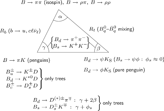
Figure 5: A brief roadmap of $B$-decay strategies for the exploration of CP violation.

3.4 How Could New Physics Enter?

Using the concept of the low-energy effective Hamiltonians introduced in Subsection 3.2, we may address this important question in a systematic manner [48]:

• NP may modify the “strength” of the SM operators through new short-distance functions which depend on the NP parameters, such as the masses of charginos, squarks, charged Higgs particles and $\tan\bar{\beta}\equiv v_{2}/v_{1}$ in the “minimal supersymmetric SM” (MSSM). The NP particles may enter in box and penguin topologies, and are “integrated out” as the $W$ boson and top quark in the SM. Consequently, the initial conditions for the renormalization-group evolution take the following form:

  $$C_{k}\to C_{k}^{\rm SM}+C_{k}^{\rm NP}.$$ (62)

  It should be emphasized that the NP pieces $C_{k}^{\rm NP}$ may also involve new CP-violating phases which are not related to the CKM matrix.

• NP may enhance the operator basis:

  $$\{Q_{k}\}\to\{Q_{k}^{\rm SM},Q_{l}^{\rm NP}\},$$ (63)

  so that operators which are not present (or strongly suppressed) in the SM may actually play an important rôle. In this case, we encounter, in general, also new sources for flavour and CP violation.

The $B$-meson system offers a variety of processes and strategies for the exploration of CP violation [12, 49], as we have illustrated in Fig. 5 through a collection of prominent examples. We see that there are processes with a very different dynamics that are – in the SM – sensitive to the same angles of the UT. Moreover, rare $B$- and $K$-meson decays [50], which originate from loop effects in the SM, provide complementary insights into flavour physics and interesting correlations with the CP-B sector; key examples are $B\to X_{s}\gamma$ and the exclusive modes $B\to K^{\ast}\gamma$, $B\to\rho\gamma$, as well as $B_{s,d}\to\mu^{+}\mu^{-}$ and $K^{+}\to\pi^{+}\nu\bar{\nu}$, $K_{\rm L}\to\pi^{0}\nu\bar{\nu}$.

In the presence of NP contributions, the subtle interplay between the different processes could well be disturbed. There are two popular avenues for NP to enter the roadmap of quark-flavour physics:

• $B^{0}_{q}$–$\bar{B}^{0}_{q}$ mixing: NP could enter through the exchange of new particles in the box diagrams, or through new contributions at the tree level, thereby leading to

  $$\Delta M_{q}=\Delta M_{q}^{\rm SM}+\Delta M_{q}^{\rm NP},\quad\phi_{q}=\phi_{q}^{\rm SM}+\phi_{q}^{\rm NP}.$$ (64)

  Whereas $\Delta M_{q}^{\rm NP}$ would affect the determination of the UT side $R_{t}$, $\phi_{q}^{\rm NP}$ would manifest itself through mixing-induced CP asymmetries. Using dimensional arguments borrowed from effective field theory [51, 52], it can be shown that $\Delta M_{q}^{\rm NP}/\Delta M_{q}^{\rm SM}\sim 1$ and $\phi_{q}^{\rm NP}/\phi_{q}^{\rm SM}\sim 1$ could – in principle – be possible for a NP scale $\Lambda_{\rm NP}$ in the TeV regime; such a pattern may also arise in specific NP scenarios. Thanks to the $B$-factory data, dramatic NP effects of this kind are already ruled out in the $B_{d}$-meson system, although the new world average for $(\sin 2\beta)_{\psi K_{\rm S}}$ could be interpreted in terms of $\phi_{q}^{\rm NP}\sim-8^{\circ}$. On the other hand, the $B_{s}$ sector is still essentially unexplored, thereby leaving a lot of hope for the LHC.

• Decay amplitudes: NP has typically a small effect if SM tree processes play the dominant rôle. However, NP could well have a significant impact on the FCNC sector: new particles may enter in penguin or box diagrams, or new FCNC contributions may even be generated at the tree level. In fact, sizeable contributions arise generically in field-theoretical estimates with $\Lambda_{\rm NP}\sim\mbox{TeV}$ [53], as well as in specific NP models. Interestingly, there are hints in the $B$-factory data that this may actually be the case.

Concerning model-dependent NP analyses, in particular SUSY scenarios have received a lot of attention; for a selection of recent studies, see Refs. [54]–[59]. Examples of other fashionable NP scenarios are left–right-symmetric models [60], scenarios with extra dimensions [61], models with an extra $Z^{\prime}$ [62], “little Higgs” scenarios [63], and models with a fourth generation [64].

The simplest extension of the SM is given by models with “minimal flavour violation” (MFV). Following the characterization given in Ref. [65], the flavour-changing processes are here still governed by the CKM matrix – in particular there are no new sources for CP violation – and the only relevant operators are those present in the SM (for an alternative definition, see Ref. [66]). Specific examples are the Two-Higgs Doublet Model II, the MSSM without new sources of flavour violation and $\tan\bar{\beta}$ not too large, models with one extra universal dimension and the simplest little Higgs models. Due to their simplicity, the extensions of the SM with MFV show several correlations between various observables, thereby allowing for powerful tests of this scenario [67]. A systematic discussion of models with “next-to-minimal flavour violation” was recently given in Ref. [68].

There are other fascinating probes for the search of NP. Important examples are the $D$-meson system [69], electric dipole moments [70], or flavour-violating charged lepton decays [71]. Since a discussion of these topics is beyond the scope of this review, the interested reader should consult the corresponding references. Let us next have a closer look at prominent $B$ decays, with a particular emphasis of the impact of NP.

     

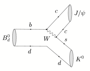
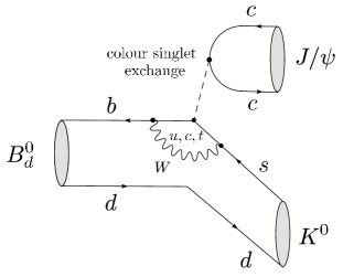
Figure 6: Feynman diagrams contributing to $B^{0}_{d}\to J/\psi K^{0}$ decays.

4 Status of Important $B$-Factory Benchmark Modes

4.1 $B^{0}_{d}\to J/\psi K_{\rm S}$

This decay has a CP-odd final state, and originates from $\bar{b}\to\bar{c}c\bar{s}$ quark-level transitions. Consequently, as we discussed in the context of the classification in Subsection 3.2, it receives contributions both from tree and from penguin topologies, as can be seen in Fig. 6. In the SM, the decay amplitude can hence be written as follows [72]:

$$A(B_{d}^{0}\to J/\psi K_{\rm S})=\lambda_{c}^{(s)}\left(A_{\rm T}^{c^{\prime}}+A_{\rm P}^{c^{\prime}}\right)+\lambda_{u}^{(s)}A_{\rm P}^{u^{\prime}}+\lambda_{t}^{(s)}A_{\rm P}^{t^{\prime}}.$$ (65)

Here the

$$\lambda_{q}^{(s)}\equiv V_{qs}V_{qb}^{\ast}$$ (66)

are CKM factors, $A_{\rm T}^{c^{\prime}}$ is the CP-conserving strong tree amplitude, while the $A_{\rm P}^{q^{\prime}}$ describe the penguin topologies with internal $q$ quarks ($q\in\{u,c,t\})$, including QCD and EW penguins; the primes remind us that we are dealing with a $\bar{b}\to\bar{s}$ transition. If we eliminate now $\lambda_{t}^{(s)}$ through (40) and apply the Wolfenstein parametrization, we obtain

$$A(B_{d}^{0}\to J/\psi K_{\rm S})\propto\left[1+\lambda^{2}ae^{i\theta}e^{i\gamma}\right],$$ (67)

where

$$ae^{i\vartheta}\equiv\left(\frac{R_{b}}{1-\lambda^{2}}\right)\left[\frac{A_{\rm P}^{u^{\prime}}-A_{\rm P}^{t^{\prime}}}{A_{\rm T}^{c^{\prime}}+A_{\rm P}^{c^{\prime}}-A_{\rm P}^{t^{\prime}}}\right]$$ (68)

is a hadronic parameter. Using now the formalism of Subsection 3.3 yields

$$\xi_{\psi K_{\rm S}}^{(d)}=+e^{-i\phi_{d}}\left[\frac{1+\lambda^{2}ae^{i\vartheta}e^{-i\gamma}}{1+\lambda^{2}ae^{i\vartheta}e^{+i\gamma}}\right].$$ (69)

Unfortunately, $ae^{i\vartheta}$, which is a measure for the ratio of the $B_{d}^{0}\to J/\psi K_{\rm S}$ penguin to tree contributions, can only be estimated with large hadronic uncertainties. However, since this parameter enters (69) in a doubly Cabibbo-suppressed way, its impact on the CP-violating observables is practically negligible. We can put this important statement on a more quantitative basis by making the plausible assumption that $a={\cal O}(\bar{\lambda})={\cal O}(0.2)={\cal O}(\lambda)$, where $\bar{\lambda}$ is a “generic” expansion parameter:

$${\cal A}^{\mbox{{\scriptsize dir}}}_{\mbox{{\scriptsize CP}}}(B_{d}\to J/\psi K_{\mbox{{\scriptsize S}}}) = 0+{\cal O}(\overline{\lambda}^{3})$$ (70)

$${\cal A}^{\mbox{{\scriptsize mix}}}_{\mbox{{\scriptsize CP}}}(B_{d}\to J/\psi K_{\mbox{{\scriptsize S}}}) = -\sin\phi_{d}+{\cal O}(\overline{\lambda}^{3})\,\stackrel{{\scriptstyle\rm SM}}{{=}}\,-\sin 2\beta+{\cal O}(\overline{\lambda}^{3}).$$ (71)

Consequently, (71) allows an essentially clean determination of $\sin 2\beta$ [47].

Since the CKM fits performed within the SM pointed to a large value of $\sin 2\beta$, $B^{0}_{d}\to J/\psi K_{\rm S}$ offered the exciting perspective of exhibiting large mixing-induced CP violation. In 2001, the measurement of ${\cal A}^{\mbox{{\scriptsize mix}}}_{\mbox{{\scriptsize CP}}}(B_{d}\to J/\psi K_{\mbox{{\scriptsize S}}})$ allowed indeed the first observation of CP violation outside the $K$-meson system [5]. The most recent data are still not showing any signal for direct CP violation in $B^{0}_{d}\to J/\psi K_{\rm S}$ within the current uncertainties, as is expected from (70). The current world average reads as follows [31]:

$${\cal A}_{\rm CP}^{\rm dir}(B_{d}\to J/\psi K_{\rm S})=0.026\pm 0.041.$$ (72)

As far as (71) is concerned, we have

$$(\sin 2\beta)_{\psi K_{\rm S}}\equiv-{\cal A}^{\mbox{{\scriptsize mix}}}_{\mbox{{\scriptsize CP}}}(B_{d}\to J/\psi K_{\mbox{{\scriptsize S}}})=\left\{\begin{array}[]{ll}0.722\pm 0.040\pm 0.023&\mbox{(BaBar \cite[cite]{[\@@bibref{}{s2b-babar}{}{}]})}\\ 0.652\pm 0.039\pm 0.020&\mbox{(Belle \cite[cite]{[\@@bibref{}{s2b-belle}{}{}]}),}\end{array}\right.$$ (73)

which gives the following world average [31]:

$$(\sin 2\beta)_{\psi K_{\rm S}}=0.687\pm 0.032.$$ (74)

Within the SM, the theoretical uncertainties are generically expected to be below the 0.01 level; significantly smaller effects are found in [75], whereas a fit performed in [76] yields a theoretical penguin uncertainty comparable to the present experimental systematic error. A possibility to control these uncertainties is provided by the $B^{0}_{s}\to J/\psi K_{\rm S}$ channel [72], which can be explored at the LHC [77].

In [51], a set of observables was introduced, which allows us to search systematically for NP contributions to the $B\to J/\psi K$ decay amplitudes. It uses also the charged $B^{\pm}\to J/\psi K^{\pm}$ decay, and is given as follows:

$${\cal B}_{\psi K}\equiv\frac{1-{\cal A}_{\psi K}}{1+{\cal A}_{\psi K}},$$ (75)

with

$${\cal A}_{\psi K}\equiv\left[\frac{\mbox{BR}(B^{+}\to J/\psi K^{+})+\mbox{BR}(B^{-}\to J/\psi K^{-})}{\mbox{BR}(B^{0}_{d}\to J/\psi K^{0})+\mbox{BR}(\bar{B}^{0}_{d}\to J/\psi\bar{K}^{0})}\right]\left[\frac{\tau_{B^{0}_{d}}}{\tau_{B^{+}}}\right],$$ (76)

and

$${\cal D}^{\pm}_{\psi K}\equiv\frac{1}{2}\left[{\cal A}_{\rm CP}^{\rm dir}(B_{d}\to J/\psi K_{\rm S})\pm{\cal A}_{\rm CP}^{\rm dir}(B^{\pm}\to J/\psi K^{\pm})\right].$$ (77)

As is discussed in detail in [49, 51], the observables ${\cal B}_{\psi K}$ and ${\cal D}^{-}_{\psi K}$ are sensitive to NP in the $I=1$ isospin sector, whereas a non-vanishing value of ${\cal D}^{+}_{\psi K}$ would signal NP in the $I=0$ isospin sector. Moreover, the NP contributions with $I=1$ are expected to be dynamically suppressed with respect to the $I=0$ case because of their flavour structure. Using the most recent $B$-factory results, we obtain

$${\cal B}_{\psi K}=-0.035\pm 0.037,\quad{\cal D}^{-}_{\psi K}=0.010\pm 0.023,\quad{\cal D}^{+}_{\psi K}=0.017\pm 0.023.$$ (78)

Consequently, NP effects of ${\cal O}(10\%)$ in the $I=1$ sector of the $B\to J/\psi K$ decay amplitudes are already disfavoured by the data for ${\cal B}_{\psi K}$ and ${\cal D}^{-}_{\psi K}$. However, since a non-vanishing value of ${\cal D}^{+}_{\psi K}$ requires also a large CP-conserving strong phase, this observable still leaves room for sizeable NP contributions to the $I=0$ sector.

Thanks to the new Belle result listed in (73), the average for $(\sin 2\beta)_{\psi K_{\rm S}}$ went down by about $1\sigma$, which is a somewhat surprising development of this summer. Consequently, the comparison of (74) with the CKM fits in the $\bar{\rho}$–$\bar{\eta}$ plane does no longer look “perfect”, as we saw in Fig. 2. In particular, if we use the value of the UT fits for $\sin 2\beta$ that follow from the experimental information for the UT sides and $\varepsilon_{K}$, $(\sin 2\beta)_{\rm UT}=0.791\pm 0.034$ [27], we obtain

$${\cal S}_{\psi K}\equiv(\sin 2\beta)_{\psi K_{\rm S}}-(\sin 2\beta)_{\rm UT}=-0.104\pm 0.047.$$ (79)

The are two limiting cases of this possible discrepancy with the KM mechanism of CP violation: NP contributions to the $B\to J/\psi K$ decay amplitudes, or NP effects entering through $B^{0}_{d}$–$\bar{B}^{0}_{d}$ mixing. Let us first illustrate the former case. Since the NP effects in the $I=1$ sector are expected to be dynamically suppressed, we consider only NP in the $I=0$ isospin sector, which implies ${\cal B}_{\psi K}={\cal D}^{-}_{\psi K}=0$, in accordance with (78). To simplify the discussion, we assume that there is effectively only a single NP contribution of this kind, so that we may write

$$A(B^{0}_{d}\to J/\psi K^{0})=A_{0}\left[1+v_{0}e^{i(\Delta_{0}+\phi_{0})}\right]=A(B^{+}\to J/\psi K^{+}).$$ (80)

Here $v_{0}$ and the CP-conserving strong phase $\Delta_{0}$ are hadronic parameters, whereas $\phi_{0}$ denotes a CP-violating phase originating beyond the SM. An interesting specific scenario falling into this category arises if the NP effects enter through EW penguins. This kind of NP has recently received a lot of attention in the context of the $B\to\pi K$ puzzle, which we shall discuss in Section 5. Also within the SM, where $\phi_{0}$ vanishes, EW penguins have a sizeable impact on the $B\to J/\psi K$ system [78]. Using factorization, the following estimate can be obtained [39]:

$$\left.v_{0}e^{i\Delta_{0}}\right|_{\rm fact}^{\rm SM}\approx-0.03.$$ (81)

In Figs. 7 (a) and (b), we show the situation in the ${\cal S}_{\psi K}$–${\cal D}^{+}_{\psi K}$ plane for $\phi_{0}=-90^{\circ}$ and $\phi_{0}=+90^{\circ}$, respectively. The contours correspond to different values of $v_{0}$, and are obtained by varying $\Delta_{0}$ between $0^{\circ}$ and $360^{\circ}$; the experimental data are represented by the diamonds with the error bars. Since factorization gives $\Delta_{0}=180^{\circ}$, as can be seen in (81), the case of $\phi_{0}=-90^{\circ}$ is disfavoured. On the other hand, in the case of $\phi_{0}=+90^{\circ}$, the experimental region can straightforwardly be reached for $\Delta_{0}$ not differing too much from the factorization result, although an enhancement of $v_{0}$ by a factor of ${\cal O}(3)$ with respect to the SM estimate in (81), which suffers from large uncertainties, would simultaneously be required in order to reach the central experimental value. Consequently, NP contributions to the EW penguin sector could, in principle, be at the origin of the possible discrepancy indicated by (79). This scenario should be carefully monitored as the data improve.

(a) (b)

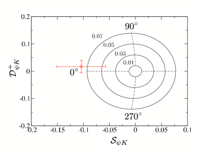
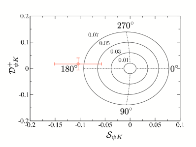
Figure 7: The situation in the ${\cal S}_{\psi K}$–${\cal D}^{+}_{\psi K}$ plane for NP contributions to the $B\to J/\psi K$ decay amplitudes in the $I=0$ isospin sector for NP phases $\phi_{0}=-90^{\circ}$ (a) and $\phi_{0}=+90^{\circ}$ (b). The diamonds with the error bars represent the averages of the current data, whereas the numbers correspond to the values of $\Delta_{0}$ and $v_{0}$.

Another explanation of (79) is provided by CP-violating NP contributions to $B^{0}_{d}$–$\bar{B}^{0}_{d}$ mixing, which affect the corresponding mixing phase as follows:

$$\phi_{d}=\phi_{d}^{\rm SM}+\phi_{d}^{\rm NP}=2\beta+\phi_{d}^{\rm NP}.$$ (82)

If we assume that the NP contributions to the $B\to J/\psi K$ decay amplitudes are negligible, the world average in (74) implies

$$\phi_{d}=(43.4\pm 2.5)^{\circ}\quad\lor\quad(136.6\pm 2.5)^{\circ}.$$ (83)

Here the latter solution would be in dramatic conflict with the CKM fits, and would require a large NP contribution to $B^{0}_{d}$–$\bar{B}^{0}_{d}$ mixing [52, 79]. Both solutions can be distinguished through the measurement of the sign of $\cos\phi_{d}$, where a positive value would select the SM-like branch. Using an angular analysis of the decay products of $B_{d}\to J/\psi[\to\ell^{+}\ell^{-}]K^{\ast}[\to\pi^{0}K_{\rm S}]$ processes, the BaBar collaboration finds [80]

$$\cos\phi_{d}=2.72^{+0.50}_{-0.79}\pm 0.27,$$ (84)

thereby favouring the solution around $\phi_{d}=43^{\circ}$. Interestingly, this picture emerges also from the first data for CP-violating effects in $B_{d}\to D^{(*)\pm}\pi^{\mp}$ modes [81], and an analysis of the $B\to\pi\pi,\pi K$ system [39], although in an indirect manner. Recently, a new method has been proposed, which makes use of the interference pattern in $D\to K_{\rm S}\pi^{+}\pi^{-}$ decays emerging from $B_{d}\to D\pi^{0}$ and similar decays [82]. The results of this method are also consistent with the SM, so that a negative value of $\cos\phi_{d}$ is now ruled out with greater than 95% confidence [83]. Since the value of $(\sin 2\beta)_{\rm UT}$ given before (79) corresponds to $\beta=(26.1\pm 1.6)^{\circ}$, (82) yields $\phi_{d}^{\rm NP}=-(8.9\pm 4.1)^{\circ}$. Consequently, the $B$-factory data do not leave too much space for CP-violating NP contributions to $B^{0}_{d}$–$\bar{B}^{0}_{d}$ mixing. On the other hand, such effects are still unexplored in $B^{0}_{s}$–$\bar{B}^{0}_{s}$ mixing, where they can nicely be probed through $B^{0}_{s}\to J/\psi\phi$ decays, which are very accessible at the LHC. For NP models that are interesting in this context, see Refs. [55, 57, 62].

The possibility of having a non-zero value of (79) could of course just be due to a statistical fluctuation. However, should it be confirmed, it could be due to CP-violating NP contributions to the $B^{0}_{d}\to J/\psi K_{\rm S}$ decay amplitude or to $B^{0}_{d}$–$\bar{B}^{0}_{d}$ mixing, as we just saw. A tool to distinguish between these avenues is provided by decays of the kind $B_{d}\to D\pi^{0},D\rho^{0},...$, which are pure “tree” decays, i.e. they do not receive any penguin contributions. If the neutral $D$ mesons are observed through their decays into CP eigenstates $D_{\pm}$, these decays allow extremely clean determinations of the “true” value of $\sin 2\beta$ [84], as we shall discuss in more detail in Subsection 7.3. In view of (79), this would be very interesting, so that detailed feasibility studies for the exploration of the $B_{d}\to D\pi^{0},D\rho^{0},...$ modes at a super-$B$ factory are strongly encouraged.

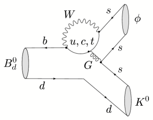
Figure 8: Feynman diagrams contributing to $B^{0}_{d}\to\phi K^{0}$ decays.

(a) (b)

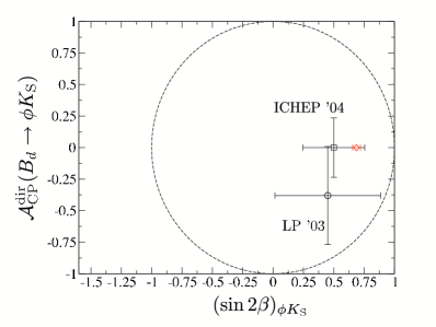
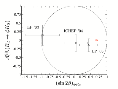
Figure 9: The time evolution of the BaBar (a) and Belle (b) data for the CP violation in $B_{d}\to\phi K_{\rm S}$. The diamonds represent the SM relations (89)–(91) with (74).

4.2 $B^{0}_{d}\to\phi K_{\rm S}$

Another important probe for the testing of the KM mechanism is offered by $B_{d}^{0}\to\phi K_{\rm S}$, which is a decay into a CP-odd final state. As can be seen in Fig. 8, it originates from $\bar{b}\to\bar{s}s\bar{s}$ transitions and is, therefore, a pure penguin mode. This decay is described by the low-energy effective Hamiltonian in (41) with $r=s$, where the current–current operators may only contribute through penguin-like contractions, which describe the penguin topologies with internal up- and charm-quark exchanges. The dominant rôle is played by the QCD penguin operators [85]. However, thanks to the large top-quark mass, EW penguins have a sizeable impact as well [86, 87]. In the SM, we may write

$$A(B_{d}^{0}\to\phi K_{\rm S})=\lambda_{u}^{(s)}\tilde{A}_{\rm P}^{u^{\prime}}+\lambda_{c}^{(s)}\tilde{A}_{\rm P}^{c^{\prime}}+\lambda_{t}^{(s)}\tilde{A}_{\rm P}^{t^{\prime}},$$ (85)

where we have applied the same notation as in Subsection 4.1. Eliminating the CKM factor $\lambda_{t}^{(s)}$ with the help of (40) yields

$$A(B_{d}^{0}\to\phi K_{\rm S})\propto\left[1+\lambda^{2}be^{i\Theta}e^{i\gamma}\right],$$ (86)

where

$$be^{i\Theta}\equiv\left(\frac{R_{b}}{1-\lambda^{2}}\right)\left[\frac{\tilde{A}_{\rm P}^{u^{\prime}}-\tilde{A}_{\rm P}^{t^{\prime}}}{\tilde{A}_{\rm P}^{c^{\prime}}-\tilde{A}_{\rm P}^{t^{\prime}}}\right].$$ (87)

Consequently, we obtain

$$\xi_{\phi K_{\rm S}}^{(d)}=+e^{-i\phi_{d}}\left[\frac{1+\lambda^{2}be^{i\Theta}e^{-i\gamma}}{1+\lambda^{2}be^{i\Theta}e^{+i\gamma}}\right].$$ (88)

The theoretical estimates of $be^{i\Theta}$ suffer from large hadronic uncertainties. However, since this parameter enters (88) in a doubly Cabibbo-suppressed way, we obtain the following expressions [78]:

$${\cal A}_{\rm CP}^{\rm dir}(B_{d}\to\phi K_{\rm S}) = 0+{\cal O}(\lambda^{2})$$ (89)

$${\cal A}_{\rm CP}^{\rm mix}(B_{d}\to\phi K_{\rm S}) = -\sin\phi_{d}+{\cal O}(\lambda^{2}),$$ (90)

where we made the plausible assumption that $b={\cal O}(1)$. On the other hand, the mixing-induced CP asymmetry of $B_{d}\to J/\psi K_{\rm S}$ measures also $-\sin\phi_{d}$, as we saw in (71). We arrive therefore at the following relation [78, 88]:

$$-(\sin 2\beta)_{\phi K_{\rm S}}\equiv{\cal A}_{\rm CP}^{\rm mix}(B_{d}\to\phi K_{\rm S})={\cal A}_{\rm CP}^{\rm mix}(B_{d}\to J/\psi K_{\rm S})+{\cal O}(\lambda^{2}),$$ (91)

which offers an interesting test of the SM. Since $B_{d}\to\phi K_{\rm S}$ is governed by penguin processes in the SM, this decay may well be affected by NP. In fact, if we assume that NP arises generically in the TeV regime, it can be shown through field-theoretical estimates that the NP contributions to $b\to s\bar{s}s$ transitions may well lead to sizeable violations of (89) and (91) [49, 53]. Moreover, this is also the case for several specific NP scenarios; for examples, see Refs. [56, 58, 59, 89].

(a) (b)

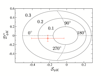
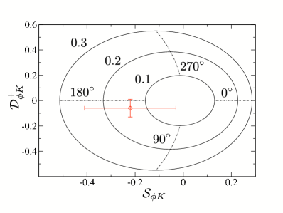
Figure 10: The situation in the ${\cal S}_{\phi K}$–${\cal D}^{+}_{\phi K}$ plane for NP contributions to the $B\to\phi K$ decay amplitudes in the $I=0$ isospin sector for NP phases $\phi_{0}=-90^{\circ}$ (a) and $\phi_{0}=+90^{\circ}$ (b). The diamonds with the error bars represent the averages of the current data, whereas the numbers correspond to the values of $\tilde{\Delta}_{0}$ and $\tilde{v}_{0}$.

In Fig. 9, we show the time evolution of the $B$-factory data for the measurements of CP violation in $B_{d}\to\phi K_{\rm S}$, using the results reported at the LP ’03 [90], ICHEP ’04 [91] and LP ’05 [92] conferences. Because of (56), the corresponding observables have to lie inside a circle with radius one around the origin, which is represented by the dashed lines. The result announced by the Belle collaboration in 2003 led to quite some excitement in the community. Meanwhile, the Babar [93] and Belle [94] results are in good agreement with each other, yielding the following averages [31]:

$${\cal A}_{\rm CP}^{\rm dir}(B_{d}\to\phi K_{\rm S})=-0.09\pm 0.14,\quad(\sin 2\beta)_{\phi K_{\rm S}}=0.47\pm 0.19.$$ (92)

If we take (74) into account, we obtain the following result for the counterpart of (79):

$${\cal S}_{\phi K}\equiv(\sin 2\beta)_{\phi K_{\rm S}}-(\sin 2\beta)_{\psi K_{\rm S}}=-0.22\pm 0.19.$$ (93)

This number still appears to be somewhat on the lower side, thereby indicating potential NP contributions to $b\to s\bar{s}s$ processes.

Further insights into the origin and the isospin structure of NP contributions can be obtained through a combined analysis of the neutral and charged $B\to\phi K$ modes with the help of observables ${\cal B}_{\phi K}$ and ${\cal D}^{\pm}_{\phi K}$ [53], which are defined in analogy to (75) and (77), respectively. The current experimental results read as follows:

$${\cal B}_{\phi K}=0.00\pm 0.08,\quad{\cal D}^{-}_{\phi K}=-0.03\pm 0.07,\quad{\cal D}^{+}_{\phi K}=-0.06\pm 0.07.$$ (94)

As in the $B\to J/\psi K$ case, ${\cal B}_{\phi K}$ and ${\cal D}^{-}_{\phi K}$ probe NP effects in the $I=1$ sector, which are expected to be dynamically suppressed, whereas ${\cal D}^{+}_{\phi K}$ is sensitive to NP in the $I=0$ sector. The latter kind of NP could also manifest itself as a non-vanishing value of (93).

In order to illustrate these effects, let us consider again the case where NP enters only in the $I=0$ isospin sector. An important example is given by EW penguins, which have a significant impact on $B\to\phi K$ decays [86]. In analogy to the discussion in Subsection 4.1, we may then write

$$A(B^{0}_{d}\to\phi K^{0})=\tilde{A}_{0}\left[1+\tilde{v}_{0}e^{i(\tilde{\Delta}_{0}+\phi_{0})}\right]=A(B^{+}\to\phi K^{+}),$$ (95)

which implies ${\cal B}_{\phi K}={\cal D}^{-}_{\phi K}=0$, in accordance with (94). The notation corresponds to the one of (80). Using the factorization approach to deal with the QCD and EW penguin contributions, we obtain the following estimate in the SM, where the CP-violating NP phase $\phi_{0}$ vanishes [39]:

$$\left.\tilde{v}_{0}e^{i\tilde{\Delta}_{0}}\right|_{\rm fact}^{\rm SM}\approx-0.2.$$ (96)

In Figs. 10 (a) and (b), we show the situation in the ${\cal S}_{\phi K}$–${\cal D}^{+}_{\phi K}$ plane for NP phases $\phi_{0}=-90^{\circ}$ and $\phi_{0}=+90^{\circ}$, respectively, and various values of $\tilde{v}_{0}$; each point of the contours is parametrized by $\tilde{\Delta}_{0}\in[0^{\circ},360^{\circ}]$. We observe that the central values of the current experimental data, which are represented by the diamonds with the error bars, can straightforwardly be accommodated in this scenario in the case of $\phi_{0}=+90^{\circ}$ for strong phases satisfying $\cos\tilde{\Delta}_{0}<0$, as in factorization. Moreover, as can also be seen in Fig. 10 (b), the EW penguin contributions would then have to be suppressed with respect to the SM estimate, which would be an interesting feature in view of the discussion of the $B\to\pi K$ puzzle and the rare decay constraints in Section 5.

It will be interesting to follow the evolution of the $B$-factory data, and to monitor also similar modes, such as $B^{0}_{d}\to\pi^{0}K_{\rm S}$ [95] and $B^{0}_{d}\to\eta^{\prime}K_{\rm S}$ [96]. For a compilation of the corresponding experimental results, see Ref. [31]; recent theoretical papers dealing with these channels can be found in Refs. [39, 97, 98, 99]. We will return to the CP asymmetries of the $B^{0}_{d}\to\pi^{0}K_{\rm S}$ channel in Section 5.

     

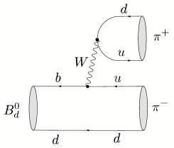
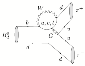
Figure 11: Feynman diagrams contributing to $B^{0}_{d}\to\pi^{+}\pi^{-}$ decays.

4.3 $B^{0}_{d}\to\pi^{+}\pi^{-}$

This decay is a transition into a CP eigenstate with eigenvalue $+1$, and originates from $\bar{b}\to\bar{u}u\bar{d}$ processes, as can be seen in Fig. 11. In analogy to (65) and (85), its decay amplitude can be written as follows [100]:

$$A(B_{d}^{0}\to\pi^{+}\pi^{-})=\lambda_{u}^{(d)}\left(A_{\rm T}^{u}+A_{\rm P}^{u}\right)+\lambda_{c}^{(d)}A_{\rm P}^{c}+\lambda_{t}^{(d)}A_{\rm P}^{t}.$$ (97)

Using again (40) to eliminate the CKM factor $\lambda_{t}^{(d)}=V_{td}V_{tb}^{\ast}$ and applying once more the Wolfenstein parametrization yields

$$A(B_{d}^{0}\to\pi^{+}\pi^{-})={\cal C}\left[e^{i\gamma}-de^{i\theta}\right],$$ (98)

where the overall normalization ${\cal C}$ and

$$de^{i\theta}\equiv\frac{1}{R_{b}}\left[\frac{A_{\rm P}^{c}-A_{\rm P}^{t}}{A_{\rm T}^{u}+A_{\rm P}^{u}-A_{\rm P}^{t}}\right]$$ (99)

are hadronic parameters. The formalism discussed in Subsection 3.3 then implies

$$\xi_{\pi^{+}\pi^{-}}^{(d)}=-e^{-i\phi_{d}}\left[\frac{e^{-i\gamma}-de^{i\theta}}{e^{+i\gamma}-de^{i\theta}}\right].$$ (100)

In contrast to the expressions (69) and (88) for the $B_{d}^{0}\to J/\psi K_{\rm S}$ and $B^{0}_{d}\to\phi K_{\rm S}$ counterparts, respectively, the hadronic parameter $de^{i\theta}$, which suffers from large theoretical uncertainties, does not enter (100) in a doubly Cabibbo-suppressed way. This feature is at the basis of the famous “penguin problem” in $B^{0}_{d}\to\pi^{+}\pi^{-}$, which was addressed in many papers (see, for instance, [101]–[106]). If the penguin contributions to this channel were negligible, i.e. $d=0$, its CP asymmetries were simply given by

$${\cal A}_{\rm CP}^{\rm dir}(B_{d}\to\pi^{+}\pi^{-}) = 0$$ (101)

$${\cal A}_{\rm CP}^{\rm mix}(B_{d}\to\pi^{+}\pi^{-}) = \sin(\phi_{d}+2\gamma)\stackrel{{\scriptstyle\rm SM}}{{=}}\sin(\underbrace{2\beta+2\gamma}_{2\pi-2\alpha})=-\sin 2\alpha.$$ (102)

Consequently, ${\cal A}_{\rm CP}^{\rm mix}(B_{d}\to\pi^{+}\pi^{-})$ would then allow us to determine $\alpha$. However, in the general case, we obtain expressions with the help of (53) and (100) of the form

$${\cal A}_{\rm CP}^{\rm dir}(B_{d}\to\pi^{+}\pi^{-}) = G_{1}(d,\theta;\gamma)$$ (103)

$${\cal A}_{\rm CP}^{\rm mix}(B_{d}\to\pi^{+}\pi^{-}) = G_{2}(d,\theta;\gamma,\phi_{d});$$ (104)

for explicit formulae, see [100]. We observe that actually the phases $\phi_{d}$ and $\gamma$ enter directly in the $B_{d}\to\pi^{+}\pi^{-}$ observables, and not $\alpha$. Consequently, since $\phi_{d}$ can be fixed through the mixing-induced CP violation in the “golden” mode $B_{d}\to J/\psi K_{\rm S}$, as we have seen in Subsection 4.1, we may use $B_{d}\to\pi^{+}\pi^{-}$ to probe $\gamma$.

The current measurements of the $B_{d}\to\pi^{+}\pi^{-}$ CP asymmetries are given as follows:

$${\cal A}_{\rm CP}^{\rm dir}(B_{d}\to\pi^{+}\pi^{-}) = \left\{\begin{array}[]{ll}-0.09\pm 0.15\pm 0.04&\mbox{(BaBar \cite[cite]{[\@@bibref{}{BaBar-Bpipi-05}{}{}]})}\\ -0.56\pm 0.12\pm 0.06&\mbox{(Belle \cite[cite]{[\@@bibref{}{Belle-Bpipi-05}{}{}]})}\end{array}\right.$$ (107)

$${\cal A}_{\rm CP}^{\rm mix}(B_{d}\to\pi^{+}\pi^{-}) = \left\{\begin{array}[]{ll}+0.30\pm 0.17\pm 0.03&\mbox{(BaBar \cite[cite]{[\@@bibref{}{BaBar-Bpipi-05}{}{}]})}\\ +0.67\pm 0.16\pm 0.06&\mbox{(Belle \cite[cite]{[\@@bibref{}{Belle-Bpipi-05}{}{}]}).}\end{array}\right.$$ (110)

The BaBar and Belle results are still not fully consistent with each other, although the experiments are now in better agreement. In [31], the following averages were obtained:

$${\cal A}_{\rm CP}^{\rm dir}(B_{d}\to\pi^{+}\pi^{-}) = -0.37\pm 0.10$$ (111)

$${\cal A}_{\rm CP}^{\rm mix}(B_{d}\to\pi^{+}\pi^{-}) = +0.50\pm 0.12.$$ (112)

The central values of these averages are remarkably stable in time. Direct CP violation at this level would require large penguin contributions with large CP-conserving strong phases, thereby indicating large non-factorizable effects.

This picture is in fact supported by the direct CP violation in $B^{0}_{d}\to\pi^{-}K^{+}$ modes that could be established by the $B$ factories in the summer of 2004 [6]. Here the BaBar and Belle results agree nicely with each other, yielding the following average [31]:

$${\cal A}_{\rm CP}^{\rm dir}(B_{d}\to\pi^{\mp}K^{\pm})=0.115\pm 0.018.$$ (113)

The diagrams contributing to $B^{0}_{d}\to\pi^{-}K^{+}$ can straightforwardly be obtained from those in Fig. 11 by just replacing the anti-down quark emerging from the $W$ boson through an anti-strange quark. Consequently, the hadronic matrix elements entering $B^{0}_{d}\to\pi^{+}\pi^{-}$ and $B^{0}_{d}\to\pi^{-}K^{+}$ can be related to one another through the $SU(3)$ flavour symmetry of strong interactions and the additional assumption that the penguin annihilation and exchange topologies contributing to $B^{0}_{d}\to\pi^{+}\pi^{-}$, which have no counterpart in $B^{0}_{d}\to\pi^{-}K^{+}$ and involve the “spectator” down quark in Fig. 11, play actually a negligible rôle [109]. Following these lines, we obtain the following relation in the SM:

$$H_{\rm BR}\equiv\underbrace{\frac{1}{\epsilon}\left(\frac{f_{K}}{f_{\pi}}\right)^{2}\left[\frac{\mbox{BR}(B_{d}\to\pi^{+}\pi^{-})}{\mbox{BR}(B_{d}\to\pi^{\mp}K^{\pm})}\right]}_{\mbox{$7.5\pm 0.7$}}=\underbrace{-\frac{1}{\epsilon}\left[\frac{{\cal A}_{\rm CP}^{\rm dir}(B_{d}\to\pi^{\mp}K^{\pm})}{{\cal A}_{\rm CP}^{\rm dir}(B_{d}\to\pi^{+}\pi^{-})}\right]}_{\mbox{$6.7\pm 2.0$}}\equiv H_{{\cal A}_{\rm CP}^{\rm dir}},$$ (114)

where

$$\epsilon\equiv\frac{\lambda^{2}}{1-\lambda^{2}}=0.053,$$ (115)

and the ratio $f_{K}/f_{\pi}=160/131$ of the kaon and pion decay constants defined through

$$\langle 0|\bar{s}\gamma_{\alpha}\gamma_{5}u|K^{+}(k)\rangle=if_{K}k_{\alpha},\quad\langle 0|\bar{d}\gamma_{\alpha}\gamma_{5}u|\pi^{+}(k)\rangle=if_{\pi}k_{\alpha}$$ (116)

describes factorizable $SU(3)$-breaking corrections. As usual, the CP-averaged branching ratios are defined as

$$\mbox{BR}\equiv\frac{1}{2}\left[\mbox{BR}(B\to f)+\mbox{BR}(\bar{B}\to\bar{f})\right].$$ (117)

In (114), we have also given the numerical values following from the data. Consequently, this relation is well satisfied within the experimental uncertainties, and does not show any anomalous behaviour. It supports therefore the SM description of the $B^{0}_{d}\to\pi^{-}K^{+}$, $B^{0}_{d}\to\pi^{+}\pi^{-}$ decay amplitudes, and our working assumptions listed before (114).

The quantities $H_{\rm BR}$ and $H_{{\cal A}_{\rm CP}^{\rm dir}}$ introduced in this relation can be written as follows:

$$H_{\rm BR}=G_{3}(d,\theta;\gamma)=H_{{\cal A}_{\rm CP}^{\rm dir}}.$$ (118)

If we complement this expression with (103) and (104), and use (see (83))

$$\phi_{d}=(43.4\pm 2.5)^{\circ},$$ (119)

we have sufficient information to determine $\gamma$, as well as $(d,\theta)$ [100, 109, 110]. In using (119), we assume that the possible discrepancy with the SM described by (79) is only due to NP in $B^{0}_{d}$–$\bar{B}^{0}_{d}$ mixing and not to effects entering through the $B^{0}_{d}\to J/\psi K_{\rm S}$ decay amplitude. As was recently shown in Ref. [99], the results following from $H_{\rm BR}$ and $H_{{\cal A}_{\rm CP}^{\rm dir}}$ give results that are in good agreement with one another. Since the avenue offered by $H_{{\cal A}_{\rm CP}^{\rm dir}}$ is cleaner than the one provided by $H_{\rm BR}$, it is preferable to use the former quantity to determine $\gamma$, yielding the following result [99]:

$$\gamma=(73.9^{+5.8}_{-6.5})^{\circ}.$$ (120)

Here a second solution around $42^{\circ}$ was discarded, which can be exclueded through an analysis of the whole $B\to\pi\pi,\pi K$ system [39]. As was recently discussed [99] (see also Refs. [109, 110]), even large non-factorizable $SU(3)$-breaking corrections have a remarkably small impact on the numerical result in (120). The value of $\gamma$ in (120) is higher than the results following from the CKM fits [26, 27]. An even larger value in the ballpark of $80^{\circ}$ was recently extracted from the $B\to\pi\pi$ data with the help of SCET [111, 112]. Performing Dalitz analyses of the neutral $D$-meson decays in $B^{\pm}\to D^{(*)}K^{\pm}$ and $B^{\pm}\to DK^{*\pm}$ transitions, the $B$ factories have obtained the following results for $\gamma$:

$$\gamma=\left\{\begin{array}[]{ll}(67\pm 28\pm 13\pm 11)^{\circ}&\mbox{BaBar \cite[cite]{[\@@bibref{}{Babar-Dal}{}{}]}}\\ (68^{+14}_{-15}\pm 13\pm 11)^{\circ}&\mbox{Belle \cite[cite]{[\@@bibref{}{Belle-Dal}{}{}]},}\end{array}\right.$$ (121)

which agree with (120), although the errors are too large to draw definite conclusions.

The interesting feature of the value of $\gamma$ in (120) is that it should not receive significant NP contributions. If we complement it with $|V_{ub}/V_{cb}|$ extracted from semi-leptonic tree-level $B$ decays, which are also very robust with respect to NP effects, we may determine the “true” UT, i.e.  the reference UT introduced in Refs. [115, 116]. Using, as in Ref. [99], the average value $|V_{ub}/V_{cb}|=0.102\pm 0.005$ (for a detailed discussion, see Ref. [27]) yields

$$\alpha_{\rm true}=(80.3^{+6.6}_{-5.9})^{\circ},\quad\beta_{\rm true}=(25.8\pm 1.3)^{\circ},$$ (122)

corresponding to $(\sin 2\beta)_{\rm true}=0.78\pm 0.03$, which is significantly larger than (74). This difference can be attributed to a non-vanishing value of the NP phase $\phi_{d}^{\rm NP}$ in (64), where $\phi_{d}^{\rm SM}$ corresponds to $2\beta_{\rm true}$. This exercise yields $\phi^{\rm NP}_{d}=-(8.2\pm 3.5)^{\circ}$ [99], in excellent accordance with the discussion in Subsection 4.1, and the recent study of Ref. [117]. Performing detailed analyses of $B^{0}_{d}\to\rho^{+}\rho^{-}$ decays, the $B$ factories have extracted the following ranges of $\alpha$:

$$\alpha=\left\{\begin{array}[]{ll}(100\pm 13)^{\circ}&\mbox{BaBar \cite[cite]{[\@@bibref{}{Babar-alph}{}{}]}}\\ (87\pm 17)^{\circ}&\mbox{Belle \cite[cite]{[\@@bibref{}{Belle-alph}{}{}]},}\end{array}\right.$$ (123)

which can be related to $\alpha_{\rm true}$ with the help of the simple relation

$$\alpha_{\rm true}=\alpha+\phi_{d}^{\rm NP}/2.$$ (124)

Comparing (122) and (123), we observe that the latter measurements seem also to prefer a negative value of $\phi^{\rm NP}_{d}$, in accordance with the discussion given above, although the current errors are of course not conclusive. Nevertheless, this pattern is interesting and should be monitored in the future as the quality of the data improves.

The decay $B^{0}_{d}\to\pi^{+}\pi^{-}$ plays also an important rôle in the next section, dealing with an analysis of the $B\to\pi K$ system.

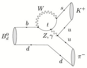
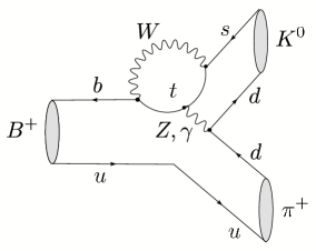
(a)       (b)      

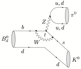
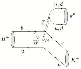
Figure 12: Examples of the colour-suppressed (a) and colour-allowed (b) EW penguin contributions to the $B\to\pi K$ system.

5 The $B\to\pi K$ Puzzle and its Relation to Rare $B$ and $K$ Decays

5.1 Preliminaries

We made already first contact with a $B\to\pi K$ decay in Subsection 4.3, the $B^{0}_{d}\to\pi^{-}K^{+}$ channel. It receives contributions both from tree and from penguin topologies. Since this decay originates from a $\bar{b}\to\bar{s}$ transition, the tree amplitude is suppressed by a CKM factor $\lambda^{2}R_{b}\sim 0.02$ with respect to the penguin amplitude. Consequently, $B^{0}_{d}\to\pi^{-}K^{+}$ is governed by QCD penguins; the tree topologies contribute only at the 20% level to the decay amplitude. The feature of the dominance of QCD penguins applies to all $B\to\pi K$ modes, which can be classified with respect to their EW penguin contributions as follows (see Fig. 12):

• In the $B^{0}_{d}\to\pi^{-}K^{+}$ and $B^{+}\to\pi^{+}K^{0}$ decays, EW penguins contribute in colour-suppressed form and are hence expected to play a minor rôle.

• In the $B^{0}_{d}\to\pi^{0}K^{0}$ and $B^{+}\to\pi^{0}K^{+}$ decays, EW penguins contribute in colour-allowed form and have therefore a significant impact on the decay amplitude, entering at the same order of magnitude as the tree contributions.

As we noted above, EW penguins offer an attractive avenue for NP to enter non-leptonic $B$ decays, which is also the case for the $B\to\pi K$ system [120, 121]. Indeed, the decays of class (b) show a puzzling pattern, which may point towards such a NP scenario. This feature emerged already in 2000 [122], when the CLEO collaboration reported the observation of the $B^{0}_{d}\to\pi^{0}K^{0}$ channel with a surprisingly prominent rate [123], and is still present in the most recent BaBar and Belle data, thereby receiving a lot of attention in the literature (see, for instance, Refs. [89] and [124]–[128]).

In the following discussion, we focus on the systematic strategy to explore the “$B\to\pi K$ puzzle” developed in Ref. [39]; all numerical results refer to the most recent analysis presented in Ref. [99]. The logical structure is very simple: the starting point is given by the values of $\phi_{d}$ and $\gamma$ in (119) and (120), respectively, and by the $B\to\pi\pi$ system, which allows us to extract a set of hadronic parameters from the data with the help of the isospin symmetry of strong interactions. Then we make, in analogy to the determination of $\gamma$ in Subsection 4.3, the following working hypotheses:

• $SU(3)$ flavour symmetry of strong interactions (but taking factorizable $SU(3)$-breaking corrections into account),

• neglect of penguin annihilation and exchange topologies,

which allow us to fix the hadronic $B\to\pi K$ parameters through their $B\to\pi\pi$ counterparts. Interestingly, we may gain confidence in these assumptions through internal consistency checks (an example is relation (114)), which work nicely within the experimental uncertainties. Having the hadronic $B\to\pi K$ parameters at hand, we can predict the $B\to\pi K$ observables in the SM. The comparison of the corresponding picture with the $B$-factory data will then guide us to NP in the EW penguin sector, involving in particular a large CP-violating NP phase. In the final step, we explore the interplay of this NP scenario with rare $K$ and $B$ decays.

5.2 Extracting Hadronic Parameters from the $B\to\pi\pi$ System

In order to fully exploit the information that is provided by the whole $B\to\pi\pi$ system, we use – in addition to the two CP-violating $B^{0}_{d}\to\pi^{+}\pi^{-}$ observables – the following ratios of CP-averaged branching ratios:

$$R_{+-}^{\pi\pi} \equiv 2\left[\frac{\mbox{BR}(B^{+}\to\pi^{+}\pi^{0})+\mbox{BR}(B^{-}\to\pi^{-}\pi^{0})}{\mbox{BR}(B_{d}^{0}\to\pi^{+}\pi^{-})+\mbox{BR}(\bar{B}_{d}^{0}\to\pi^{+}\pi^{-})}\right]=2.04\pm 0.28$$ (125)

$$R_{00}^{\pi\pi} \equiv 2\left[\frac{\mbox{BR}(B_{d}^{0}\to\pi^{0}\pi^{0})+\mbox{BR}(\bar{B}_{d}^{0}\to\pi^{0}\pi^{0})}{\mbox{BR}(B_{d}^{0}\to\pi^{+}\pi^{-})+\mbox{BR}(\bar{B}_{d}^{0}\to\pi^{+}\pi^{-})}\right]=0.58\pm 0.13.$$ (126)

The pattern of the experimental numbers in these expressions came as quite a surprise, as the central values calculated in QCDF gave $R_{+-}^{\pi\pi}=1.24$ and $R_{00}^{\pi\pi}=0.07$ [124]. As discussed in detail in [39], this “$B\to\pi\pi$ puzzle” can straightforwardly be accommodated in the SM through large non-factorizable hadronic interference effects, i.e. does not point towards NP. For recent SCET analyses, see Refs. [112, 129, 130].

Using the isospin symmetry of strong interactions, we can write

$$R_{+-}^{\pi\pi}=F_{1}(d,\theta,x,\Delta;\gamma),\quad R_{00}^{\pi\pi}=F_{2}(d,\theta,x,\Delta;\gamma),$$ (127)

where $xe^{i\Delta}$ is another hadronic parameter, which was introduced in [39]. Using now, in addition, the CP-violating observables in (103) and (104), we arrive at the following set of haronic parameters:

$$d=0.52^{+0.09}_{-0.09},\quad\theta=(146^{+7.0}_{-7.2})^{\circ},\quad x=0.96^{+0.13}_{-0.14},\quad\Delta=-(53^{+18}_{-26})^{\circ}.$$ (128)

In the extraction of these quantites, also the EW penguin effects in the $B\to\pi\pi$ system are included [131, 132], although these topologies have a tiny impact [95]. Let us emphasize that the results for the hadronic parameters listed above, which are consistent with the picture emerging in the analyses of other authors (see, e.g., Refs. [41, 133]), are essentially clean and serve as a testing ground for calculations within QCD-related approaches. For instance, in recent QCDF [134] and PQCD [135] analyses, the following numbers were obtained:

$$\left.d\right|_{\rm QCDF}=0.29\pm 0.09,\quad\left.\theta\right|_{\rm QCDF}=-\left(171.4\pm 14.3\right)^{\circ},$$ (129)

$$\left.d\right|_{\rm PQCD}=0.23^{+0.07}_{-0.05},\quad+139^{\circ}<\left.\theta\right|_{\rm PQCD}<+148^{\circ},$$ (130)

which depart significantly from the pattern in (128) that is implied by the data.

Finally, we can predict the CP asymmetries of the decay $B_{d}\to\pi^{0}\pi^{0}$:

$${\cal A}_{\rm CP}^{\rm dir}(B_{d}\to\pi^{0}\pi^{0})=-0.30^{+0.48}_{-0.26},\quad{\cal A}_{\rm CP}^{\rm mix}(B_{d}\to\pi^{0}\pi^{0})=-0.87^{+0.29}_{-0.19}.$$ (131)

The current experimental value for the direct CP asymmetry is given as follows [31]:

$${\cal A}_{\rm CP}^{\rm dir}(B_{d}\to\pi^{0}\pi^{0})=-0.28^{+0.40}_{-0.39}.$$ (132)

Consequently, no stringent test of the corresponding prediction in (131) is provided at this stage, although the indicated agreement is encouraging.

5.3 Analysis of the $B\to\pi K$ System

Let us begin the analysis of the $B\to\pi K$ system by having a closer look at the modes of class (a) introduced above, $B_{d}\to\pi^{\mp}K^{\pm}$ and $B^{\pm}\to\pi^{\pm}K$, which are only marginally affected by EW penguin contributions. We used the banching ratio and direct CP asymmetry of the former channel already in the $SU(3)$ relation (114), which is nicely satisfied by the current data, and in the extraction of $\gamma$ with the help of the CP-violating $B_{d}\to\pi^{+}\pi^{-}$ observables, yielding the value in (120). The $B_{d}\to\pi^{\mp}K^{\pm}$ modes provide the CP-violating asymmetry

$${\cal A}_{\rm CP}^{\rm dir}(B^{\pm}\to\pi^{\pm}K)\equiv\frac{\mbox{BR}(B^{+}\to\pi^{+}K^{0})-\mbox{BR}(B^{-}\to\pi^{-}\bar{K}^{0})}{\mbox{BR}(B^{+}\to\pi^{+}K^{0})+\mbox{BR}(B^{-}\to\pi^{-}\bar{K}^{0})}=0.02\pm 0.04,$$ (133)

and enter in the following ratio [136]:

$$R\equiv\left[\frac{\mbox{BR}(B_{d}^{0}\to\pi^{-}K^{+})+\mbox{BR}(\bar{B}_{d}^{0}\to\pi^{+}K^{-})}{\mbox{BR}(B^{+}\to\pi^{+}K^{0})+\mbox{BR}(B^{-}\to\pi^{-}\bar{K}^{0})}\right]\frac{\tau_{B^{+}}}{\tau_{B^{0}_{d}}}=0.86\pm 0.06;$$ (134)

the numerical values refer again to the most recent compilation in [31]. The $B^{+}\to\pi^{+}K^{0}$ channel involves another hadronic parameter, $\rho_{\rm c}e^{i\theta_{\rm c}}$, which cannot be determined through the $B\to\pi\pi$ data [131, 137, 138]:

$$A(B^{+}\to\pi^{+}K^{0})=-P^{\prime}\left[1+\rho_{\rm c}e^{i\theta_{\rm c}}e^{i\gamma}\right];$$ (135)

the overall normalization $P^{\prime}$ cancels in (133) and (134). Usually, it is assumed that the parameter $\rho_{\rm c}e^{i\theta_{\rm c}}$ can be neglected. In this case, the direct CP asymmetry in (133) vanishes, and $R$ can be calculated through the $B\to\pi\pi$ data with the help of the assumptions specified in Subsection 5.1:

$$R|_{\rm SM}=0.963^{+0.019}_{-0.022}.$$ (136)

This numerical result is $1.6\sigma$ larger than the experimental value in (134). As was discussed in detail in [139], the experimental range for the direct CP asymmetry in (133) and the first direct signals for the $B^{\pm}\to K^{\pm}K$ decays favour a value of $\theta_{\rm c}$ around $0^{\circ}$. This feature allows us to essentially resolve the small discrepancy concerning $R$ for values of $\rho_{\rm c}$ around 0.05. The remaining small numerical difference between the calculated value of $R$ and the experimental result, if confirmed by future data, could be due to (small) colour-suppressed EW penguins, which enter $R$ as well [39]. As was recently discussed in Ref. [99], even large non-factorizable $SU(3)$-breaking effects would have a small impact on the predicted value of $R$. In view of these results, it would not be a surprise to see an increase of the experimental value of $R$ in the future.

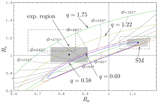
Figure 13: The current situation in the $R_{\rm n}$–$R_{\rm c}$ plane: the shaded areas indicate the experimental and SM $1\sigma$ ranges, while the lines show the theory predictions for the central values of the hadronic parameters and various values of $q$ with $\phi\in[0^{\circ},360^{\circ}]$.

Let us now turn to the $B^{+}\to\pi^{0}K^{+}$ and $B^{0}_{d}\to\pi^{0}K^{0}$ channels, which are the $B\to\pi K$ modes with significant contributions from EW penguin topologies. The key observables for the exploration of these modes are the following ratios of their CP-averaged branching ratios [122, 131]:

$$R_{\rm c}\equiv 2\left[\frac{\mbox{BR}(B^{+}\to\pi^{0}K^{+})+\mbox{BR}(B^{-}\to\pi^{0}K^{-})}{\mbox{BR}(B^{+}\to\pi^{+}K^{0})+\mbox{BR}(B^{-}\to\pi^{-}\bar{K}^{0})}\right]=1.01\pm 0.09$$ (137)

$$R_{\rm n}\equiv\frac{1}{2}\left[\frac{\mbox{BR}(B_{d}^{0}\to\pi^{-}K^{+})+\mbox{BR}(\bar{B}_{d}^{0}\to\pi^{+}K^{-})}{\mbox{BR}(B_{d}^{0}\to\pi^{0}K^{0})+\mbox{BR}(\bar{B}_{d}^{0}\to\pi^{0}\bar{K}^{0})}\right]=0.83\pm 0.08,$$ (138)

where the overall normalization factors of the decay amplitudes cancel, as in (134). In order to describe the EW penguin effects, both a parameter $q$, which measures the strength of the EW penguins with respect to tree-like topologies, and a CP-violating phase $\phi$ are introduced. In the SM, this phase vanishes, and $q$ can be calculated with the help of the $SU(3)$ flavour symmetry, yielding a value of $0.69\times 0.086/|V_{ub}/V_{cb}|=0.58$ [140]. Following the strategy described above yields the following SM predictions:

$$R_{\rm c}|_{\rm SM}=1.15\pm 0.05,\quad R_{\rm n}|_{\rm SM}=1.12\pm 0.05,$$ (139)

where in particular the value of $R_{\rm n}$ does not agree with the experimental number, which is a manifestation of the $B\to\pi K$ puzzle. As was recently discussed in Ref. [99], the internal consistency checks of the working assumptions listed in Subsection 5.1 are currently satisfied at the level of $25\%$, and can be systematically improved through better data. A detailed study of the numerical predictions in (139) (and those given below) shows that their sensitivity on non-factorizable $SU(3)$-breaking effects of this order of magnitude is surprisingly small. Consequently, it is very exciting to speculate that NP effects in the EW penguin sector, which are described effectively through $(q,\phi)$, are at the origin of the $B\to\pi K$ puzzle. Following Ref. [39], we show the situation in the $R_{\rm n}$–$R_{\rm c}$ plane in Fig. 13, where – for the convenience of the reader – also the experimental range and the SM predictions at the time of the original analysis of Ref. [39] are indicated through the dashed rectangles. We observe that although the central values of $R_{\rm n}$ and $R_{\rm c}$ have slightly moved towards each other, the puzzle is as prominent as ever. The experimental region can now be reached without an enhancement of $q$, but a large CP-violating phase $\phi$ of the order of $-90^{\circ}$ is still required:

$$q=0.99\,^{+0.66}_{-0.70},\quad\phi=-(94\,^{+16}_{-17})^{\circ}.$$ (140)

Interestingly, $\phi$ of the order of $+90^{\circ}$ can now also bring us rather close to the experimental range of $R_{\rm n}$ and $R_{\rm c}$.

An interesting probe of the NP phase $\phi$ is also provided by the CP violation in the decay $B^{0}_{d}\to\pi^{0}K_{\rm S}$. Within the SM, the corresponding observables are expected to satisfy the following relations [95]:

$${\cal A}_{\rm CP}^{\rm dir}(B_{d}\!\to\!\pi^{0}K_{\rm S})\approx 0,\quad{\cal A}_{\rm CP}^{\rm mix}(B_{d}\!\to\!\pi^{0}K_{\rm S})\approx{\cal A}_{\rm CP}^{\rm mix}(B_{d}\!\to\!\psi K_{\rm S}).$$ (141)

The most recent Belle [94] and BaBar [141] measurements of these quantities are in agreement with each other, and lead to the following averages [31]:

$${\cal A}_{\rm CP}^{\rm dir}(B_{d}\!\to\!\pi^{0}K_{\rm S}) = -0.02\pm 0.13$$ (142)

$${\cal A}_{\rm CP}^{\rm mix}(B_{d}\!\to\!\pi^{0}K_{\rm S}) = -0.31\pm 0.26\equiv-(\sin 2\beta)_{\pi^{0}K_{\rm S}}.$$ (143)

Taking (74) into account yields

$$\Delta S\equiv(\sin 2\beta)_{\pi^{0}K_{\rm S}}-(\sin 2\beta)_{\psi K_{\rm S}}=-0.38\pm 0.26,$$ (144)

which may indicate a sizeable deviation of the experimentally measured value of $(\sin 2\beta)_{\pi^{0}K_{\rm S}}$ from $(\sin 2\beta)_{\psi K_{\rm S}}$, and is therefore one of the recent hot topics. Since the strategy developed in Ref. [39] allows us also to predict the CP-violating observables of the $B^{0}_{d}\to\pi^{0}K_{\rm S}$ channel both within the SM and within our scenario of NP, it allows us to address this issue, yielding

$${\cal A}_{\rm CP}^{\rm dir}(B_{d}\!\to\!\pi^{0}K_{\rm S})|_{\rm SM}=0.06^{+0.09}_{-0.10},\qquad\Delta S|_{\rm SM}=0.13\pm 0.05,$$ (145)

$${\cal A}_{\rm CP}^{\rm dir}(B_{d}\!\to\!\pi^{0}K_{\rm S})|_{\rm NP}=0.01\,^{+0.14}_{-0.18},\qquad\Delta S|_{\rm NP}=0.27\,^{+0.05}_{-0.09},$$ (146)

where the NP results refer to the EW penguin parameters in (140). Consequently, $\Delta S$ is found to be positive in the SM. In the literature, values of $\Delta S|_{\rm SM}\sim 0.04$–$0.08$ can be found, which were obtained – in contrast to (145) – with the help of dynamical approaches such as QCDF [98] and SCET [112]. Moreover, bounds were derived with the help of the $SU(3)$ flavour symmetry [142]. Looking at (146), we see that the modified parameters $(q,\phi)$ in (140) imply an enhancement of $\Delta S$ with respect to the SM case. Consequently, the best values of $(q,\phi)$ that are favoured by the measurements of $R_{\rm n,c}$ make the potential ${\cal A}_{\rm CP}^{\rm mix}(B_{d}\!\to\!\pi^{0}K_{\rm S})$ discrepancy even larger than in the SM.

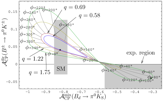
Figure 14: The situation in the ${\cal A}_{\rm CP}^{\rm mix}(B_{d}\to\pi^{0}K_{\rm S})$–${\cal A}_{\rm CP}^{\rm dir}(B^{\pm}\to\pi^{0}K^{\pm})$ plane: the shaded regions represent the experimental and SM $1\sigma$ ranges, while the lines show the theory predictions for the central values of the hadronic parameters and various values of $q$ with $\phi\in[0^{\circ},360^{\circ}]$.

There is one CP asymmetry of the $B\to\pi K$ system left, which is measured as

$${\cal A}_{\rm CP}^{\rm dir}(B^{\pm}\to\pi^{0}K^{\pm})=-0.04\pm 0.04.$$ (147)

In the limit of vanishing colour-suppressed tree and EW penguin topologies, it is expected to be equal to the direct CP asymmetry of the $B_{d}\to\pi^{\mp}K^{\pm}$ modes. Since the experimental value of the latter asymmetry in (113) does not agree with (147), the direct CP violation in $B^{\pm}\to\pi^{0}K^{\pm}$ has also received a lot of attention. The lifted colour suppression described by the large value of $x$ in (128) could, in principle, be responsible for a non-vanishing difference between (113) and (147),

$$\Delta A\equiv{\cal A}_{\rm CP}^{\rm dir}(B^{\pm}\to\pi^{0}K^{\pm})-{\cal A}_{\rm CP}^{\rm dir}(B_{d}\to\pi^{\mp}K^{\pm})\,\stackrel{{\scriptstyle{\rm exp}}}{{=}}-0.16\pm 0.04.$$ (148)

However, applying once again the strategy described above yields

$${\cal A}_{\rm CP}^{\rm dir}(B^{\pm}\to\pi^{0}K^{\pm})|_{\rm SM}=0.04\,^{+0.09}_{-0.07},$$ (149)

so that the SM still prefers a positive value of this CP asymmetry; the NP scenario characterized by (140) corresponds to

$${\cal A}_{\rm CP}^{\rm dir}(B^{\pm}\to\pi^{0}K^{\pm})|_{\rm NP}=0.09\,^{+0.20}_{-0.16}.$$ (150)

In view of the large uncertainties, no stringent test is provided at this point. Nevertheless, it is tempting to play a bit with the CP asymmetries of the $B^{\pm}\to\pi^{0}K^{\pm}$ and $B_{d}\to\pi^{0}K_{\rm S}$ decays. In Fig. 14, we show the situation in the ${\cal A}_{\rm CP}^{\rm mix}(B_{d}\to\pi^{0}K_{\rm S})$–${\cal A}_{\rm CP}^{\rm dir}(B^{\pm}\to\pi^{0}K^{\pm})$ plane for various values of $q$ with $\phi\in[0^{\circ},360^{\circ}]$. We see that these observables seem to show a preference for positive values of $\phi$ around $+90^{\circ}$. As we noted above, in this case, we can also get rather close to the experimental region in the $R_{\rm n}$–$R_{\rm c}$ plane. It is now interesting to return to the discussion of the NP effects in the $B\to\phi K$ system given in Subsection 4.2. In our scenario of NP in the EW penguin sector, we have just to identify the CP-violating phase $\phi_{0}$ in (95) with the NP phase $\phi$ [39]. Unfortunately, we cannot determine the hadronic $B\to\phi K$ parameters $\tilde{v}_{0}$ and $\tilde{\Delta}_{0}$ through the $B\to\pi\pi$ data as in the case of the $B\to\pi K$ system. However, if we take into account that $\tilde{\Delta}_{0}=180^{\circ}$ in factorization and look at Fig. 10, we see again that the case of $\phi\sim+90^{\circ}$ would be favoured by the data for ${\cal S}_{\phi K}$. Alternatively, in the case of $\phi\sim-90^{\circ}$, $\tilde{\Delta}_{0}\sim 0^{\circ}$ would be required to accommodate a negative value of ${\cal S}_{\phi K}$, which appears unlikely. Interestingly, a similar comment applies to the $B\to J/\psi K$ observables shown in Fig. 7, although here a dramatic enhancement of the EW penguin parameter $v_{0}$ relative to the SM estimate would be simultaneously needed to reach the central experimental values, in contract to the reduction of $\tilde{v}_{0}$ in the $B\to\phi K$ case. In view of rare decay constraints, the behaviour of the $B\to\phi K$ parameter $\tilde{v}_{0}$ appears much more likely, thereby supporting the assumption after (119).

5.4 The Interplay with Rare $K$ and $B$ Decays and Future Scenarios

In order to explore the implications of the $B\to\pi K$ puzzle for rare $K$ and $B$ decays, we assume that the NP enters the EW penguin sector through $Z^{0}$ penguins with a new CP-violating phase. This scenario was already considered in the literature, where model-independent analyses and studies within SUSY can be found [143, 144]. In the strategy discussed here, the short-distance function $C$ characterizing the $Z^{0}$ penguins is determined through the $B\to\pi K$ data [145]. Performing a renormalization-group analysis yields

$$C(\bar{q})=2.35~{}\bar{q}e^{i\phi}-0.82\quad\mbox{with}\quad\bar{q}=q\left[\frac{|V_{ub}/V_{cb}|}{0.086}\right].$$ (151)

Evaluating then the relevant box-diagram contributions in the SM and using (151), the short-distance functions

$$X=2.35~{}\bar{q}e^{i\phi}-0.09\quad\mbox{and}\quad Y=2.35~{}\bar{q}e^{i\phi}-0.64$$ (152)

can also be calculated, which govern the rare $K$, $B$ decays with $\nu\bar{\nu}$ and $\ell^{+}\ell^{-}$ in the final states, respectively. In the SM, we have $C=0.79$, $X=1.53$ and $Y=0.98$, with vanishing CP-violating phases. An analysis along these lines shows that the value of $(q,\phi)$ in (140), which is preferred by the $B\to\pi K$ observables $R_{\rm n,c}$, requires the following lower bounds for $X$ and $Y$ [99]:

$$|X|_{\rm min}\approx|Y|_{\rm min}\approx 2.2,$$ (153)

which appear to violate the $95\%$ probability upper bounds

$$X\leq 1.95,\quad Y\leq 1.43$$ (154)

that were recently obtained within the context of MFV [146]. Although we have to deal with CP-violating NP phases in our scenario, which goes therefore beyond the MFV framework, a closer look at $B\to X_{s}\ell^{+}\ell^{-}$ shows that the upper bound on $|Y|$ in (154) is difficult to avoid if NP enters only through EW penguins and the operator basis is the same as in the SM. A possible solution to the clash between (153) and (154) would be given by more complicated NP scenarios [99]. However, unless a specific model is chosen, the predictive power is then significantly reduced. For the exploration of the NP effects in rare decays, we will therefore not follow this avenue.

Quantity	SM	Scen A	Scen B	Scen C	Experiment
$R_{\rm n}$	1.12	$0.88$	1.03	1	$0.83\pm 0.08$
$R_{\rm c}$	1.15	$0.96$	1.13	1	$1.01\pm 0.09$
${\cal A}_{\rm CP}^{\rm dir}(B^{\pm}\!\to\!\pi^{0}K^{\pm})$	0.04	$0.07$	0.06	0.02	$-0.04\pm 0.04$
${\cal A}_{\rm CP}^{\rm dir}(B_{d}\!\to\!\pi^{0}K_{\rm S})$	0.06	$0.04$	0.03	0.09	$-0.02\pm 0.13$
${\cal A}_{\rm CP}^{\rm mix}(B_{d}\!\to\!\pi^{0}K_{\rm S})$	$-0.82$	$-0.89$	$-0.91$	$-0.70$	$-0.31\pm 0.26$
$\Delta S$	0.13	0.21	0.22	0.01	$-0.38\pm 0.26$
$\Delta A$	$-0.07$	$-0.04$	$-0.05$	$-0.09$	$-0.16\pm 0.04$

Table 1: The $B\to\pi K$ observables for the three scenarios introduced in the text.

Decay	SM	Scen A	Scen B	Scen C	Exp. bound (90% C.L.)
$\mbox{BR}(K^{+}\to\pi^{+}\nu\bar{\nu})/10^{-11}$	$9.3$	$2.7$	$8.3$	$8.4$	$(14.7^{+13.0}_{-8.9})$
$\mbox{BR}(K_{\rm L}\to\pi^{0}\nu\bar{\nu})/10^{-11}$	$4.4$	$11.6$	$27.9$	$7.2$	$<2.9\times 10^{4}$
$\mbox{BR}(K_{\rm L}\to\pi^{0}e^{+}e^{-})/10^{-11}$	$3.6$	$4.6$	$7.1$	$4.9$	$<28$
$\mbox{BR}(B\to X_{s}\nu\bar{\nu})/10^{-5}$	$3.6$	$2.8$	$4.8$	$3.3$	$<64$
$\mbox{BR}(B_{s}\to\mu^{+}\mu^{-})/10^{-9}$	$3.9$	$9.2$	$9.1$	$7.0$	$<1.5\times 10^{2}$
$\mbox{BR}(K_{\rm L}\to\mu^{+}\mu^{-})_{\rm SD}/10^{-9}$	$0.9$	$0.9$	$0.001$	$0.6$	$<2.5$

Table 2: Rare decay branching ratios for the three scenarios introduced in the text. We will have a closer look at the $B_{s}\to\mu^{+}\mu^{-}$ channel in Subsection 7.5.

Using an only slightly more generous bound on $|Y|$ by imposing $\left|Y\right|\leq 1.5$ and taking only those values of (140) that satisfy the constraint $\left|Y\right|=1.5$ yields

$$q=0.48\pm 0.07,\quad\phi=-(93\pm 17)^{\circ},$$ (155)

corresponding to a modest suppression of $q$ relative to its updated SM value of $0.58$. It is interesting to investigate the impact of various modifications of $(q,\phi)$, which allow us to satisfy the bounds in (154), for the $B\to\pi K$ observables and rare decays. To this end, three scenarios for the possible future evolution of the measurements of $R_{\rm n}$ and $R_{\rm c}$ were introduced in [99]:

• Scenario A: $q=0.48$, $\phi=-93^{\circ}$, which is in accordance with the currrent rare decay bounds and the $B\to\pi K$ data (see (155)).

• Scenario B: $q=0.66$, $\phi=-50^{\circ}$, which yields an increase of $R_{\rm n}$ to 1.03, and some interesting effects in rare decays. This could, for example, happen if radiative corrections to the $B_{d}^{0}\to\pi^{-}K^{+}$ branching ratio enhance $R_{\rm n}$ [147], though this alone would probably account for only about $5\%$.

• Scenario C: here it is assumed that $R_{\rm n}=R_{\rm c}=1$, which corresponds to $q=0.54$ and $\phi=61^{\circ}$. The positive sign of $\phi$ distinguishes this scenario strongly from the others.

The patterns of the observables of the $B\to\pi K$ and rare decays corresponding to these scenarios are collected in Tables 1 and 2, respectively. We observe that the $K\to\pi\nu\bar{\nu}$ modes, which are theoretically very clean (for a recent review, see Ref. [148]), offer a particularly interesting probe for the different scenarios. Concerning the observables of the $B\to\pi K$ system, ${\cal A}_{\rm CP}^{\rm mix}(B_{d}\!\to\!\pi^{0}K_{\rm S})$ is very interesting: this CP asymmetry is found to be very large in Scenarios A and B, where the NP phase $\phi$ is negative. On the other hand, the positive sign of $\phi$ in Scenario C brings ${\cal A}_{\rm CP}^{\rm mix}(B_{d}\!\to\!\pi^{0}K_{\rm S})$ closer to the data, in agreement with the features discussed in Subsection 5.3. A similar comment applies to the direct CP asymmetry of $B^{\pm}\to\pi^{0}K^{\pm}$.

In view of the large uncertainties, unfortunately no definite conclusions on the presence of NP can be drawn at this stage. However, the possible anomalies in the $B\to\pi K$ system complemented with the one in $B\to\phi K$ may actually indicate the effects of a modified EW penguin sector with a large CP-violating NP phase. As we just saw, rare $K$ and $B$ decays have an impressive power to reveal such a kind of NP. Let us finally stress that the analysis of the $B\to\pi\pi$ modes, which signals large non-factorizable effects, and the determination of the UT angle $\gamma$ described above are not affected by such NP effects. It will be interesting to monitor the evolution of the corresponding data with the help of the strategy discussed above.

6 A New Territory: $b\to d$ Penguins

6.1 Preliminaries

Another hot topic which emerged recently is the exploration of $b\to d$ penguin processes. The non-leptonic decays belonging to this category, which are mediated by $b\to d\bar{s}s$ quark transitions (see the classification in Subsection 3.2), are now coming within experimental reach at the $B$ factories. A similar comment applies to the radiative decays originating from $b\to d\gamma$ processes, whereas $b\to d\ell^{+}\ell^{-}$ modes are still far from being accessible. The $B$ factories are therefore just entering a new territory, which is still essentially unexplored. Let us now have a closer look at the corresponding processes.

6.2 A Prominent Example: $B^{0}_{d}\to K^{0}\bar{K}^{0}$

The Feynman diagrams contributing to this decay can straightforwardly be obtained from those for $B^{0}_{d}\to\phi K^{0}$ shown in Fig. 8 by replacing the anti-strange quark emerging from the $W$ boson through an anti-down quark. The $B^{0}_{d}\to K^{0}\bar{K}^{0}$ decay is described by the low-energy effective Hamiltonian in (41) with $r=d$, where the current–current operators may only contribute through penguin-like contractions, corresponding to the penguin topologies with internal up- and charm-quark exchanges. The dominant rôle is played by QCD penguins; since EW penguins contribute only in colour-suppressed form, they have a minor impact on $B^{0}_{d}\to K^{0}\bar{K}^{0}$, in contrast to the case of $B^{0}_{d}\to\phi K^{0}$, where they may also contribute in colour-allowed form.

If apply the notation introduced in Section 4, make again use of the unitarity of the CKM matrix and apply the Wolfenstein parametrization, we may write the $B^{0}_{d}\to K^{0}\bar{K}^{0}$ amplitude as follows:

$$A(B^{0}_{d}\to K^{0}\bar{K}^{0})=\lambda^{3}A(\tilde{A}_{\rm P}^{t}-\tilde{A}_{\rm P}^{c})\left[1-\rho_{K\!K}e^{i\theta_{K\!K}}e^{i\gamma}\right],$$ (156)

where

$$\rho_{K\!K}e^{i\theta_{K\!K}}\equiv R_{b}\left[\frac{\tilde{A}_{\rm P}^{t}-\tilde{A}_{\rm P}^{u}}{\tilde{A}_{\rm P}^{t}-\tilde{A}_{\rm P}^{c}}\right].$$ (157)

This expression allows us to calculate the CP-violating asymmetries with the help of the formulae given in Subsection 3.3, taking the following form:

$${\cal A}_{\rm CP}^{\rm dir}(B_{d}\to K^{0}\bar{K}^{0}) = D_{1}(\rho_{K\!K},\theta_{K\!K};\gamma)$$ (158)

$${\cal A}_{\rm CP}^{\rm mix}(B_{d}\to K^{0}\bar{K}^{0}) = D_{2}(\rho_{K\!K},\theta_{K\!K};\gamma,\phi_{d}).$$ (159)

Let us assume, for a moment, that the penguin contributions are dominated by top-quark exchanges. In this case, (157) simplifies as

$$\rho_{K\!K}e^{i\theta_{K\!K}}\to R_{b}.$$ (160)

Since the CP-conserving strong phase $\theta_{K\!K}$ vanishes in this limit, the direct CP violation in $B^{0}_{d}\to K^{0}\bar{K}^{0}$ vanishes, too. Moreover, if we take into account that $\phi_{d}=2\beta$ in the SM and use trigonometrical relations which can be derived for the UT, we find that also the mixing-induced CP asymmetry would be zero. These features suggest an interesting test of the $b\to d$ flavour sector of the SM (see, for instance, [149]). However, contributions from penguins with internal up- and charm-quark exchanges are expected to yield sizeable CP asymmetries in $B_{d}^{0}\to K^{0}\bar{K}^{0}$ even within the SM, so that the interpretation of these effects is much more complicated [150]; these contributions contain also possible long-distance rescattering effects [151], which are often referred to as “GIM” and “charming” penguins and received recently a lot of attention [152].

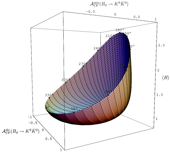
Figure 15: Illustration of the surface in the ${\cal A}_{\rm CP}^{\rm dir}$–${\cal A}_{\rm CP}^{\rm mix}$–$\langle B\rangle$ observable space characterizing the $B^{0}_{d}\to K^{0}\bar{K}^{0}$ decay in the SM. The intersecting lines on the surface correspond to constant values of $\rho_{K\!K}$ and $\theta_{K\!K}$; the numbers on the fringe indicate the value of $\theta_{K\!K}$, while the fringe itself is defined by $\rho_{K\!K}=1$.

Despite this problem, interesting insights can be obtained through the $B^{0}_{d}\to K^{0}\bar{K}^{0}$ observables [153]. By the time the CP-violating asymmetries in (158) and (159) can be measured, also the angle $\gamma$ of the UT will be reliably known, in addition to the $B^{0}_{d}$–$\bar{B}^{0}_{d}$ mixing phase $\phi_{d}$. The experimental values of the CP asymmetries can then be converted into $\rho_{K\!K}$ and $\theta_{K\!K}$, in analogy to the $B\to\pi\pi$ discussion in Subsection 5.2. Although these quantities are interesting to obtain insights into the $B\to\pi K$ parameter $\rho_{\rm c}e^{i\theta_{\rm c}}$ (see (135)) through $SU(3)$ arguments, and can be compared with theoretical predictions, for instance, those of QCDF, PQCD or SCET, they do not provide – by themselves – a test of the SM description of the FCNC processes mediating the decay $B^{0}_{d}\to K^{0}\bar{K}^{0}$. However, so far, we have not yet used the information offered by the CP-averaged branching ratio of this channel. It takes the following form:

$$\mbox{BR}(B_{d}\to K^{0}\bar{K}^{0})=\frac{\tau_{B_{d}}}{16\pi M_{B_{d}}}\times\Phi_{KK}\times|\lambda^{3}A\,\tilde{A}_{\rm P}^{tc}|^{2}\langle B\rangle,$$ (161)

where $\Phi_{KK}$ denotes a two-body phase-space factor, $\tilde{A}_{\rm P}^{tc}\equiv\tilde{A}_{\rm P}^{t}-\tilde{A}_{\rm P}^{c}$, and

$$\langle B\rangle\equiv 1-2\rho_{K\!K}\cos\theta_{K\!K}\cos\gamma+\rho_{K\!K}^{2}.$$ (162)

If we now use $\phi_{d}$ and the SM value of $\gamma$, we may characterize the decay $B^{0}_{d}\to K^{0}\bar{K}^{0}$ – within the SM – through a surface in the observable space of ${\cal A}_{\rm CP}^{\rm dir}$, ${\cal A}_{\rm CP}^{\rm mix}$ and $\langle B\rangle$. In Fig. 15, we show this surface, where each point corresponds to a given value of $\rho_{K\!K}$ and $\theta_{K\!K}$. It should be emphasized that this surface is theoretically clean since it relies only on the general SM parametrization of $B^{0}_{d}\to K^{0}\bar{K}^{0}$. Consequently, should future measurements give a value in observable space that should not lie on the SM surface, we would have immediate evidence for NP contributions to $\bar{b}\to\bar{d}s\bar{s}$ processes.

Looking at Fig. 15, we see that $\langle B\rangle$ takes an absolute minimum. Indeed, if we keep $\rho_{K\!K}$ and $\theta_{K\!K}$ as free parameters in (162), we find

$$\langle B\rangle\geq\sin^{2}\gamma,$$ (163)

which yields a strong lower bound because of the favourably large value of $\gamma$. Whereas the direct and mixing-induced CP asymmetries can be extracted from a time-dependent rate asymmetry (see (52)), the determination of $\langle B\rangle$ requires further information to fix the overall normalization factor involving the penguin amplitude $\tilde{A}_{\rm P}^{tc}$. The strategy developed in Ref. [39] offers the following two avenues, using data for

• $B\to\pi\pi$ decays, i.e. $b\to d$ transitions, implying the following lower bound:

  $$\mbox{BR}(B_{d}\to K^{0}\bar{K}^{0})_{\rm min}=\Xi^{K}_{\pi}\times\left(1.39\,^{+1.54}_{-0.95}\right)\times 10^{-6},$$ (164)

• $B\to\pi K$ decays, i.e. $b\to s$ transitions, which are complemented by the $B\to\pi\pi$ system to determine a small correction, implying the following lower bound:

  $$\mbox{BR}(B_{d}\to K^{0}\bar{K}^{0})_{\rm min}=\Xi^{K}_{\pi}\times\left(1.36\,^{+0.18}_{-0.21}\right)\times 10^{-6}.$$ (165)

Here factorizable $SU(3)$-breaking corrections are included, as is made explicit through

$$\Xi^{K}_{\pi}=\left[\frac{f_{0}^{K}}{0.331}\frac{0.258}{f_{0}^{\pi}}\right]^{2},$$ (166)

where the numerical values for the $B\to K,\pi$ form factors $f_{0}^{K,\pi}$ refer to a recent light-cone sum-rule analysis [154]. At the time of the derivation of these bounds, the $B$ factories reported an experimental upper bound of $\mbox{BR}(B_{d}\to K^{0}\bar{K}^{0})<1.5\times 10^{-6}$ (90% C.L.). Consequently, the theoretical lower bounds given above suggested that the observation of this channel should just be ahead of us. Subsequently, the first signals were indeed announced, in accordance with (164) and (165):

$$\mbox{BR}(B_{d}\to K^{0}\bar{K}^{0})=\left\{\begin{array}[]{ll}(1.19^{+0.40}_{-0.35}\pm 0.13)\times 10^{-6}&\mbox{(BaBar \cite[cite]{[\@@bibref{}{BaBar-BKK}{}{}]}),}\\ (0.8\pm 0.3\pm 0.1)\times 10^{-6}&\mbox{(Belle \cite[cite]{[\@@bibref{}{Belle-BKK}{}{}]}).}\end{array}\right.$$ (167)

The SM description of $B^{0}_{d}\to K^{0}\bar{K}^{0}$ has thus successfully passed its first test. However, the experimental errors are still very large, and the next crucial step – a measurement of the CP asymmetries – is still missing. Using QCDF, an analysis of NP effects in this channel was recently performed in the minimal supersymmetric standard model [157]. For further aspects of $B^{0}_{d}\to K^{0}\bar{K}^{0}$, the reader is referred to Ref. [153].

6.3 Radiative $b\to d$ Penguin Decays: $\bar{B}\to\rho\gamma$

Another important tool to explore $b\to d$ penguins is provided by $\bar{B}\to\rho\gamma$ modes. In the SM, these decays are described by a Hamiltonian with the following structure [32]:

$${\cal H}_{\rm eff}^{b\to d\gamma}=\frac{G_{\rm F}}{\sqrt{2}}\sum_{j=u,c}\!V_{jd}^{\ast}V_{jb}\left[\sum_{k=1}^{2}C_{k}Q_{k}^{jd}\!+\!\sum_{k=3}^{8}C_{k}Q_{k}^{d}\right].$$ (168)

Here the $Q_{1,2}^{jd}$ denote the current–current operators, whereas the $Q_{3\ldots 6}^{d}$ are the QCD penguin operators, which govern the decay $\bar{B}^{0}_{d}\to K^{0}\bar{K}^{0}$ together with the penguin-like contractions of $Q_{1,2}^{cd}$ and $Q_{1,2}^{ud}$. In contrast to these four-quark operators,

$$Q_{7,8}^{d}=\frac{1}{8\pi^{2}}m_{b}\bar{d}_{i}\sigma^{\mu\nu}(1+\gamma_{5})\left\{eb_{i}F_{\mu\nu},\,g_{\rm s}T^{a}_{ij}b_{j}G^{a}_{\mu\nu}\right\}$$ (169)

are electro- and chromomagnetic penguin operators. The most important contributions to $\bar{B}\to\rho\gamma$ originate from $Q_{1,2}^{jd}$ and $Q_{7,8}^{d}$, whereas the QCD penguin operators play only a minor rôle, in contrast to $\bar{B}^{0}_{d}\to K^{0}\bar{K}^{0}$. If we use again the unitarity of the CKM matrix and apply the Wolfenstein parametrization, we may write

$$A(\bar{B}\to\rho\gamma)=c_{\rho}\lambda^{3}A{\cal P}_{tc}^{\rho\gamma}\left[1-\rho_{\rho\gamma}e^{i\theta_{\rho\gamma}}e^{-i\gamma}\right],$$ (170)

where $c_{\rho}=1/\sqrt{2}$ and 1 for $\rho=\rho^{0}$ and $\rho^{\pm}$, respectively, ${\cal P}_{tc}^{\rho\gamma}\equiv{\cal P}_{t}^{\rho\gamma}-{\cal P}_{c}^{\rho\gamma}$, and

$$\rho_{\rho\gamma}e^{i\theta_{\rho\gamma}}\equiv R_{b}\left[\frac{{\cal P}_{t}^{\rho\gamma}-{\cal P}_{u}^{\rho\gamma}}{{\cal P}_{t}^{\rho\gamma}-{\cal P}_{c}^{\rho\gamma}}\right].$$ (171)

Here we follow our previous notation, i.e. the ${\cal P}_{j}^{\rho\gamma}$ are strong amplitudes with the following interpretation: ${\cal P}_{u}^{\rho\gamma}$ and ${\cal P}_{c}^{\rho\gamma}$ refer to the matrix elements of $\sum_{k=1}^{2}C_{k}Q_{k}^{ud}$ and $\sum_{k=1}^{2}C_{k}Q_{k}^{cd}$, respectively, whereas ${\cal P}_{t}^{\rho\gamma}$ corresponds to $-\sum_{k=3}^{8}C_{k}Q_{k}^{d}$. Consequently, ${\cal P}_{u}^{\rho\gamma}$ and ${\cal P}_{c}^{\rho\gamma}$ describe the penguin topologies with internal up- and charm-quark exchanges, respectively, whereas ${\cal P}_{t}^{\rho\gamma}$ corresponds to the penguins with the top quark running in the loop. Let us note that (170) refers to a given photon helicity. However, the $b$ quarks couple predominantly to left-handed photons in the SM, so that the right-handed amplitude is usually neglected [158]; we shall return to this point below. Comparing (170) with (156), we observe that the structure of both amplitudes is the same. In analogy to $\rho_{K\!K}e^{i\theta_{K\!K}}$, $\rho_{\rho\gamma}e^{i\theta_{\rho\gamma}}$ may also be affected by long-distance effects, which represent a key uncertainty of $\bar{B}\to\rho\gamma$ decays [77, 158].

If we replace all down quarks in (168) by strange quarks, we obtain the Hamiltonian for $b\to s\gamma$ processes, which are already well established experimentally [31]:

$$\mbox{BR}(B^{\pm}\to K^{\ast\pm}\gamma) = (40.3\pm 2.6)\times 10^{-6}$$ (172)

$$\mbox{BR}(B_{d}^{0}\to K^{\ast 0}\gamma) = (40.1\pm 2.0)\times 10^{-6}.$$ (173)

In analogy to (170), we may write

$$A(\bar{B}\!\to\!K^{\ast}\!\gamma)\!=-\!\frac{\lambda^{3}\!A{\cal P}_{tc}^{K^{\ast}\!\gamma}}{\sqrt{\epsilon}}\!\left[1\!+\!\epsilon\rho_{K\!^{\ast}\!\gamma}e^{i\theta_{K\!^{\ast}\!\gamma}}e^{-i\!\gamma}\right]\!,$$ (174)

where $\epsilon$ was introduced in (115). Thanks to the smallness of $\epsilon$, the parameter $\rho_{K\!^{\ast}\gamma}e^{i\theta_{K\!^{\ast}\gamma}}$ plays an essentially negligible rôle for the $\bar{B}\to K^{\ast}\gamma$ transitions.

Let us have a look at the charged decays $B^{\pm}\to\rho^{\pm}\gamma$ and $B^{\pm}\to K^{\ast\pm}\gamma$ first. If we consider their CP-averaged branching ratios, we obtain

$$\frac{\mbox{BR}(B^{\pm}\to\rho^{\pm}\gamma)}{\mbox{BR}(B^{\pm}\to K^{\ast\pm}\gamma)}=\epsilon\left[\frac{\Phi_{\rho\gamma}}{\Phi_{K\!^{\ast}\gamma}}\right]\left|\frac{{\cal P}_{tc}^{\rho\gamma}}{{\cal P}_{tc}^{K\!^{\ast}\gamma}}\right|^{2}H^{\rho\gamma}_{K\!^{\ast}\gamma},$$ (175)

where $\Phi_{\rho\gamma}$ and $\Phi_{K\!^{\ast}\gamma}$ denote phase-space factors, and

$$H^{\rho\gamma}_{K\!^{\ast}\gamma}\equiv\frac{1-2\rho_{\rho\gamma}\cos\theta_{\rho\gamma}\cos\gamma+\rho_{\rho\gamma}^{2}}{1+2\epsilon\rho_{K\!^{\ast}\gamma}\cos\theta_{K\!^{\ast}\gamma}\cos\gamma+\epsilon^{2}\rho_{K\!^{\ast}\gamma}^{2}}.$$ (176)

Since $B^{\pm}\to\rho^{\pm}\gamma$ and $B^{\pm}\to K^{\ast\pm}\gamma$ are related through the interchange of all down and strange quarks, the $U$-spin flavour symmetry of strong interactions allows us to relate the corresponding hadronic amplitudes to each other; the $U$-spin symmetry is an $SU(2)$ subgroup of the full $SU(3)_{\rm F}$ flavour-symmetry group, which relates down and strange quarks in the same manner as the conventional strong isospin symmetry relates down and up quarks. Following these lines, we obtain

$$|{\cal P}_{tc}^{\rho\gamma}|=|{\cal P}_{tc}^{K\!^{\ast}\gamma}|$$ (177)

$$\rho_{\rho\gamma}e^{i\theta_{\rho\gamma}}=\rho_{K\!^{\ast}\gamma}e^{i\theta_{K\!^{\ast}\gamma}}\equiv\rho e^{i\theta}.$$ (178)

Although we may determine the ratio of the penguin amplitudes $|{\cal P}_{tc}|$ in (175) with the help of (177) – up to $SU(3)$-breaking effects to be discussed below – we are still left with the dependence on $\rho$ and $\theta$. However, keeping $\rho$ and $\theta$ as free parameters, it can be shown that $H^{\rho\gamma}_{K\!^{\ast}\gamma}$ satisfies the following relation [159]:

$$H^{\rho\gamma}_{K\!^{\ast}\gamma}\geq\left[1-2\epsilon\cos^{2}\gamma+{\cal O}(\epsilon^{2})\right]\sin^{2}\gamma,$$ (179)

where the term linear in $\epsilon$ gives a shift of about $1.9\%$.

Concerning possible $SU(3)$-breaking effects to (178), they may only enter this tiny correction and are negligible for our analysis. On the other hand, the $SU(3)$-breaking corrections to (177) have a sizeable impact. Following [160, 161], we write

$$\left[\frac{\Phi_{\rho\gamma}}{\Phi_{K\!^{\ast}\gamma}}\right]\left|\frac{{\cal P}_{tc}^{\rho\gamma}}{{\cal P}_{tc}^{K\!^{\ast}\gamma}}\right|^{2}=\left[\frac{M_{B}^{2}-M_{\rho}^{2}}{M_{B}^{2}-M_{K^{\ast}}^{2}}\right]^{3}\zeta^{2},$$ (180)

where $\zeta=F_{\rho}/F_{K^{\ast}}$ is the $SU(3)$-breaking ratio of the $B^{\pm}\to\rho^{\pm}\gamma$ and $B^{\pm}\to K^{\ast\pm}\gamma$ form factors; a light-cone sum-rule analysis gives $\zeta^{-1}=1.31\pm 0.13$ [162]. Consequently, (179) and (180) allow us to convert the measured $B^{\pm}\to K^{\ast\pm}\gamma$ branching ratio (172) into a lower SM bound for $\mbox{BR}(B^{\pm}\to\rho^{\pm}\gamma)$ with the help of (175) [159]:

$$\mbox{BR}(B^{\pm}\to\rho^{\pm}\gamma)_{\rm min}=\left(1.02\,^{+0.27}_{-0.23}\right)\times 10^{-6}.$$ (181)

A similar kind of reasoning holds also for the $U$-spin pairs $B^{\pm}\to K^{\pm}K,\pi^{\pm}K$ and $B^{\pm}\to K^{\pm}K^{\ast},\pi^{\pm}K^{\ast}$, where the following lower bounds can be derived [159]:

$$\mbox{BR}(B^{\pm}\!\to\!K^{\pm}K)_{\rm min}\!\! = \!\!\Xi^{K}_{\pi}\!\times\!\left(1.69\,^{+0.21}_{-0.24}\right)\!\times\!10^{-6}$$ (182)

$$\mbox{BR}(B^{\pm}\!\to\!K^{\pm}K^{\ast})_{\rm min}\!\! = \!\!\Xi^{K}_{\pi}\!\times\!\left(0.68\,^{+0.11}_{-0.13}\right)\!\times\!10^{-6},$$ (183)

with $\Xi^{K}_{\pi}$ given in (166). Thanks to the most recent $B$-factory data, we have now also evidence for $B^{\pm}\to K^{\pm}K$ decays:

$$\mbox{BR}(B^{\pm}\!\to\!K^{\pm}K)=\left\{\begin{array}[]{ll}(1.5\pm 0.5\pm 0.1)\times 10^{-6}&\mbox{(BaBar \cite[cite]{[\@@bibref{}{BaBar-BKK}{}{}]})}\\ (1.0\pm 0.4\pm 0.1)\times 10^{-6}&\mbox{(Belle \cite[cite]{[\@@bibref{}{Belle-BKK}{}{}]}),}\end{array}\right.$$ (184)

whereas the upper limit of $5.3\times 10^{-6}$ for $B^{\pm}\to K^{\pm}K^{\ast}$ still leaves a lot of space. Obviously, we may also consider the $B^{\pm}\to K^{\ast\pm}K,\rho^{\pm}K$ system [159]. However, since currently only the upper bound $\mbox{BR}(B^{\pm}\to\rho^{\pm}K)<48\times 10^{-6}$ is available, we cannot yet give a number for the lower bound on $\mbox{BR}(B^{\pm}\to K^{\ast\pm}K)$. Experimental analyses of these modes are strongly encouraged.

Let us now turn to $\bar{B}^{0}_{d}\to\rho^{0}\gamma$, which receives contributions from exchange and penguin annihilation topologies that are not present in $\bar{B}^{0}_{d}\to\bar{K}^{\ast 0}\gamma$; in the case of $B^{\pm}\to\rho^{\pm}\gamma$ and $B^{\pm}\to K^{\ast\pm}\gamma$, which are related by the $U$-spin symmetry, there is a one-to-one correspondence of topologies. Making the plausible assumption that the topologies involving the spectator quarks play a minor rôle, and taking the factor of $c_{\rho^{0}}=1/\sqrt{2}$ in (170) into account, the counterpart of (181) is given by

$$\mbox{BR}(B_{d}\to\rho^{0}\gamma)_{\rm min}=\left(0.51\,^{+0.13}_{-0.11}\right)\times 10^{-6}.$$ (185)

At the time of the derivation of the lower bounds for the $B\to\rho\gamma$ branching ratios given above, the following experimental upper bounds ($90\%$ C.L.) were available:

$$\mbox{BR}(B^{\pm}\to\rho^{\pm}\gamma)<\left\{\begin{array}[]{ll}1.8\times 10^{-6}&\mbox{(BaBar \cite[cite]{[\@@bibref{}{Babar-Brhogamma-bound}{}{}]})}\\ 2.2\times 10^{-6}&\mbox{(Belle \cite[cite]{[\@@bibref{}{Belle-Brhogamma-bound}{}{}]})}\\ \end{array}\right.$$ (186)

$$\mbox{BR}(B_{d}\to\rho^{0}\gamma)<\left\{\begin{array}[]{ll}0.4\times 10^{-6}&\mbox{(BaBar \cite[cite]{[\@@bibref{}{Babar-Brhogamma-bound}{}{}]})}\\ 0.8\times 10^{-6}&\mbox{(Belle \cite[cite]{[\@@bibref{}{Belle-Brhogamma-bound}{}{}]}).}\end{array}\right.$$ (187)

Consequently, it was expected that the $\bar{B}\to\rho\gamma$ modes should soon be discovered at the $B$ factories [159]. Indeed, the Belle collaboration reported recently the first observation of $b\to d\gamma$ processes [165]:

$$\mbox{BR}(B^{\pm}\to\rho^{\pm}\gamma) = \left(0.55^{+0.43+0.12}_{-0.37-0.11}\right)\times 10^{-6}$$ (188)

$$\mbox{BR}(B_{d}\to\rho^{0}\gamma) = \left(1.17^{+0.35+0.09}_{-0.31-0.08}\right)\times 10^{-6}$$ (189)

$$\mbox{BR}(B\to(\rho,\omega)\gamma) = \left(1.34^{+0.34+0.14}_{-0.31-0.10}\right)\times 10^{-6},$$ (190)

which was one of the hot topics of the 2005 summer conferences [166]. These measurements still suffer from large uncertainties, and the pattern of the central values of (188) and (189) would be in conflict with the expectation following from the isospin symmetry. It will be interesting to follow the evolution of the data. The next important conceptual step would be the measurement of the corresponding CP-violating observables, though this is still in the distant future.

An alternative avenue to confront the data for the $B\to\rho\gamma$ branching ratios with the SM is provided by converting them into information on the side $R_{t}$ of the UT. To this end, the authors of Refs. [160, 161] use also (180), and calculate the CP-conserving (complex) parameter $\delta a$ entering $\rho_{\rho\gamma}e^{i\theta_{\rho\gamma}}=R_{b}\left[1+\delta a\right]$ in the QCDF approach. The corresponding result, which favours a small impact of $\delta a$, takes leading and next-to-leading order QCD corrections into account and holds to leading order in the heavy-quark limit [161]. In view of the remarks about possible long-distance effects made above and the $B$-factory data for the $B\to\pi\pi$ system, which indicate large corrections to the QCDF picture for non-leptonic $B$ decays into two light pseudoscalar mesons (see Subsection 5.2), it is, however, not obvious that the impact of $\delta a$ is actually small. The advantage of the bound following from (179) is that it is – by construction – not affected by $\rho_{\rho\gamma}e^{i\theta_{\rho\gamma}}$ at all.

6.4 General Lower Bounds for $b\to d$ Penguin Processes

Interestingly, the bounds discussed above are actually realizations of a general, model-independent bound that can be derived in the SM for $b\to d$ penguin processes [159]. If we consider such a decay, $\bar{B}\to\bar{f}_{d}$, we may – in analogy to (156) and (170) – write

$$A(\bar{B}\to\bar{f}_{d})=A^{(0)}_{d}\left[1-\rho_{d}e^{i\theta_{d}}e^{-i\gamma}\right],$$ (191)

so that the CP-averaged amplitude square is given as follows:

$$\langle|A(B\to f_{d})|^{2}\rangle=|A^{(0)}_{d}|^{2}\left[1-2\rho_{d}\cos\theta_{d}\cos\gamma+\rho_{d}^{2}\right].$$ (192)

In general, $\rho_{d}$ and $\theta_{d}$ depend on the point in phase space considered. Consequently, the expression

$$\mbox{BR}(B\to f_{d})=\tau_{B}\left[\sum_{\rm Pol}\int\!\!d\,{\rm PS}\,\langle|A(B\to f_{d})|^{2}\rangle\right]$$ (193)

for the CP-averaged branching ratio, where the sum runs over possible polarization configurations of $f_{d}$, does not factorize into $|A^{(0)}_{d}|^{2}$ and $[1-2\rho_{d}\cos\theta_{d}\cos\gamma+\rho_{d}^{2}]$ as in the case of the two-body decays considered above. However, if we keep $\rho_{d}$ and $\theta_{d}$ as free, “unknown” parameters at any given point in phase space, we obtain

$$\langle|A(B\to f_{d})|^{2}\rangle\geq|A^{(0)}_{d}|^{2}\sin^{2}\gamma,$$ (194)

which implies

$$\mbox{BR}(B\to f_{d})\geq\tau_{B}\left[\sum_{\rm Pol}\int\!\!d\,{\rm PS}\,|A^{(0)}_{d}|^{2}\right]\sin^{2}\gamma.$$ (195)

In order to deal with the term in square brackets, we use a $b\to s$ penguin decay $\bar{B}\to\bar{f}_{s}$, which is the counterpart of $\bar{B}\to\bar{f}_{d}$ in that the corresponding CP-conserving strong amplitudes can be related to one another through the $SU(3)$ flavour symmetry. In analogy to (174), we may then write

$$A(\bar{B}\to\bar{f}_{s})=-\frac{A^{(0)}_{s}}{\sqrt{\epsilon}}\left[1+\epsilon\rho_{s}e^{i\theta_{s}}e^{-i\gamma}\right].$$ (196)

If we neglect the term proportional to $\epsilon$ in the square bracket, we arrive at

$$\frac{\mbox{BR}(B\to f_{d})}{\mbox{BR}(B\to f_{s})}\geq\epsilon\left[\frac{\sum_{\rm Pol}\int\!d\,{\rm PS}\,|A^{(0)}_{d}|^{2}}{\sum_{\rm Pol}\int\!d\,{\rm PS}\,|A^{(0)}_{s}|^{2}}\right]\sin^{2}\gamma.$$ (197)

Apart from the tiny $\epsilon$ correction, which gave a shift of about $1.9\%$ in (179), (197) is valid exactly in the SM. If we now apply the $SU(3)$ flavour symmetry, we obtain

$$\frac{\sum_{\rm Pol}\int\!d\,{\rm PS}\,|A^{(0)}_{d}|^{2}}{\sum_{\rm Pol}\int\!d\,{\rm PS}\,|A^{(0)}_{s}|^{2}}\stackrel{{\scriptstyle SU(3)_{\rm F}}}{{\longrightarrow}}1.$$ (198)

Since $\sin^{2}\gamma$ is favourably large in the SM and the decay $\bar{B}\to\bar{f}_{s}$ will be measured before its $b\to d$ counterpart – simply because of the CKM enhancement – (197) provides strong lower bounds for $\mbox{BR}(B\to f_{d})$.

It is instructive to return briefly to $B\to\rho\gamma$. If we look at (197), we observe immediately that the assumption that these modes are governed by a single photon helicity is no longer required. Consequently, (181) and (185) are actually very robust with respect to this issue, which may only affect the $SU(3)$-breaking corrections to a small extend. This feature is interesting in view of the recent discussion in [167], where the photon polarization in $B\to\rho\gamma$ and $B\to K^{\ast}\gamma$ decays was critically analyzed.

We can now also derive a bound for the $B^{\pm}\to K^{\ast\pm}K^{\ast},\rho^{\pm}K^{\ast}$ system, where we have to sum in (197) over three polarization configurations of the vector mesons. The analysis of the $SU(3)$-breaking corrections is more involved than in the case of the decays considered above, and the emerging lower bound of $\mbox{BR}(B^{\pm}\to K^{\ast\pm}K^{\ast})_{\rm min}\sim 0.6\times 10^{-6}$ is still very far from the experimental upper bound of $71\times 10^{-6}$. Interestingly, the theoretical lower bound would be reduced by $\sim 0.6$ in the strict $SU(3)$ limit, i.e. would be more conservative [159]. A similar comment applies to (164), (165) and (182), (183). On the other hand, the $B\to\rho\gamma$ bounds in (181) and (185) would be enhanced by $\sim 1.7$ in this case. However, here the theoretical situation is more favourable since we have not to rely on the factorization hypothesis to deal with the $SU(3)$-breaking effects as in the case of the non-leptonic decays.

Let us finally come to another application of (197), which is offered by decays of the kind $\bar{B}\to\pi\ell^{+}\ell^{-}$ and $\bar{B}\to\rho\ell^{+}\ell^{-}$. It is well known that the $\rho_{d}$ terms complicate the interpretation of the corresponding data considerably [77]; the bound offers SM tests that are not affected by these contributions. The structure of the $b\to d\ell^{+}\ell^{-}$ Hamiltonian is similar to (168), but involves the additional operators

$$Q_{9,10}=\frac{\alpha}{2\pi}(\bar{\ell}\ell)_{\rm V\!,\,A}(\bar{d}_{i}b_{i})_{\rm V-A}.$$ (199)

The $b\to s\ell^{+}\ell^{-}$ modes $\bar{B}\to K\ell^{+}\ell^{-}$ and $\bar{B}\to K^{\ast}\ell^{+}\ell^{-}$ were already observed at the $B$ factories, with branching ratios at the $0.6\times 10^{-6}$ and $1.4\times 10^{-6}$ levels [31], respectively, and received considerable theoretical attention (see, e.g., [168]). For the application of (197), the charged decay combinations $B^{\pm}\to\pi^{\pm}\ell^{+}\ell^{-},K^{\pm}\ell^{+}\ell^{-}$ and $B^{\pm}\to\rho^{\pm}\ell^{+}\ell^{-},K^{\ast\pm}\ell^{+}\ell^{-}$ are suited best since the corresponding decay pairs are related to each other through the $U$-spin symmetry [169]. The numbers given above suggest

$$\mbox{BR}(B^{\pm}\to\pi^{\pm}\ell^{+}\ell^{-}),\quad\mbox{BR}(B^{\pm}\to\rho^{\pm}\ell^{+}\ell^{-})\mathrel{\hbox{\hbox to0.0pt{\hbox{\lower 4.0pt\hbox{$\sim$}}\hss}\hbox{$>$}}}10^{-8},$$ (200)

thereby leaving the exploration of these $b\to d$ penguin decays for the more distant future. Detailed studies of the associated $SU(3)$-breaking corrections are engouraged. By the time the $B^{\pm}\to\pi^{\pm}\ell^{+}\ell^{-}$, $\rho^{\pm}\ell^{+}\ell^{-}$ modes will come within experimental reach, we will hopefully have a good picture of these effects.

It will be interesting to confront all of these bounds with experimental data. In the case of the non-leptonic $B_{d}\to K^{0}\bar{K}^{0}$, $B^{\pm}\to K^{\pm}K$ modes and their radiative $B\to\rho\gamma$ counterparts, they have already provided a first successful test of the SM description of the corresponding FCNC processes, although the uncertainties are still very large in view of the fact that we are just at the beginning of the experimental exploration of these channels. A couple of other non-leptonic decays of this kind may just be around the corner. It would be exciting if some bounds were significantly violated through destructive interference between SM and NP contributions. Since the different decay classes are governed by different operators, we could actually encounter surprises!

7 A Key Target of $B$-Decay Studies in the LHC Era: $B_{s}$ Mesons

7.1 Preliminaries

First insights into the $B_{s}$ system could already be obtained through the LEP experiments (CERN) and SLD (SLAC) [170]. Since the currently operating $e^{+}e^{-}$ $B$ factories run at the $\Upsilon(4S)$ resonance, which decays only into $B_{u,d}$ but not into $B_{s}$ mesons, the $B_{s}$ system cannot be explored by the BaBar and Belle experiments. On the other hand, plenty of $B_{s}$ mesons will be produced at hadron colliders. After important steps at the Tevatron, the physics potential of the $B_{s}$-meson system can then be fully exploited at the LHC, in particular by the LHCb experiment [77, 171].

In the SM, the $B^{0}_{s}$–$\bar{B}^{0}_{s}$ oscillations are expected to be much faster than their $B_{d}$-meson counterparts, and could so far not be observed. Using the data of the LEP experiments, SLD and the Tevatron, only lower bounds on $\Delta M_{s}$ could be obtained. The most recent world average reads as follows [172]:

$$\Delta M_{s}>16.6\,\mbox{ps}^{-1}\,\mbox{(90\% C.L.)}.$$ (201)

The mass difference $\Delta M_{s}$ plays an important rôle in the CKM fits discussed in Subsection 2.5. Let us now have a closer look at this topic. Following the discussion given in Section 3, the mass difference of the $B_{q}$ mass eigenstates satisfies the following relation in the SM:

$$\Delta M_{q}\propto M_{B_{q}}\hat{B}_{B_{q}}f_{B_{q}}^{2}|V_{tq}^{\ast}V_{tb}|^{2},$$ (202)

where $M_{B_{q}}\equiv[M_{\rm H}^{(q)}+M_{\rm L}^{(q)}]/2$, and the factor of $\hat{B}_{B_{q}}f_{B_{q}}^{2}$ involving a “bag” parameter and the $B_{q}$ decay constant defined in analogy to (116) arises from the parametrization of the hadronic matrix element of the $(\bar{b}q)_{\rm V-A}(\bar{b}q)_{\rm V-A}$ operator of the low-energy effective Hamiltonian describing $B^{0}_{q}$–$\bar{B}^{0}_{q}$ mixing. Looking at (202), we see that knowledge of these non-perturbative hadronic parameters, which typically comes from lattice [12, 173] or QCD sum-rule calculations [174], allows us to determine $|V_{td}|$, which can then be converted into the UT side $R_{t}$ with the help of (19), as $|V_{cb}|=A\lambda^{2}$ can be determined through semi-leptonic $B$ decays [12]. On the other hand, the Wolfenstein expansion allows us also to derive the relation

$$R_{t}\equiv\frac{1}{\lambda}\left|\frac{V_{td}}{V_{cb}}\right|=\frac{1}{\lambda}\left|\frac{V_{td}}{V_{ts}}\right|\left[1+{\cal O}(\lambda^{2})\right].$$ (203)

Consequently, we may – up to corrections entering at the $\lambda^{2}$ level – determine $R_{t}$ through

$$\frac{\Delta M_{d}}{\Delta M_{s}}=\left[\frac{M_{B_{d}}}{M_{B_{s}}}\right]\left[\frac{\hat{B}_{B_{d}}}{\hat{B}_{B_{s}}}\right]\left[\frac{f_{B_{d}}}{f_{B_{s}}}\right]^{2}\left|\frac{V_{td}}{V_{ts}}\right|^{2}\,\Rightarrow\,\left|\frac{V_{td}}{V_{ts}}\right|=\xi\sqrt{\left[\frac{M_{B_{s}}}{M_{B_{d}}}\right]\left[\frac{\Delta M_{d}}{\Delta M_{s}}\right]},$$ (204)

where

$$\xi\equiv\frac{\sqrt{\hat{B}_{s}}f_{B_{s}}}{\sqrt{\hat{B}_{d}}f_{B_{d}}}$$ (205)

equals 1 in the strict $SU(3)$ limit. The evaluation of the $SU(3)$-breaking corrections entering $\xi$ is an important aspect of lattice QCD; recent studies give [173]

$$\xi=1.23\pm 0.06.$$ (206)

In comparison with the determination of $R_{t}$ through the absolute value of $\Delta M_{d}$, the advantage of (204) is that the hadronic parameters enter only through $SU(3)$-breaking corrections. Moreover, the CKM factor $A$, the short-distance QCD corrections, and the Inami–Lim function $S_{0}(x_{t})$ cancel in this expression. Thanks to the latter feature, the determination of $R_{t}$ with the help of (204) is not only valid in the SM, but also in the NP scenarios with MFV, in contrast to the extraction using only the information about $\Delta M_{d}$ [67]. As can be see in Fig. 2, the main implication of the experimental lower bound for $\Delta M_{s}$ is $\gamma\mathrel{\hbox{\hbox to0.0pt{\hbox{\lower 4.0pt\hbox{$\sim$}}\hss}\hbox{$<$}}}90^{\circ}$.

In Subsection 3.1 we saw that the width difference $\Delta\Gamma_{d}$ is negligibly small, whereas its $B_{s}$ counterpart is expected to be sizeable. As was recently reviewed in Ref. [175], the current theoretical status of these quantities is given as follows:

$$\frac{|\Delta\Gamma_{d}|}{\Gamma_{d}}=(3\pm 1.2)\times 10^{-3},\quad\frac{|\Delta\Gamma_{s}|}{\Gamma_{s}}=0.12\pm 0.05.$$ (207)

The width difference $\Delta\Gamma_{s}$ may provide interesting studies of CP violation through “untagged” $B_{s}$ rates [176]–[180], which are defined as

$$\langle\Gamma(B_{s}(t)\to f)\rangle\equiv\Gamma(B^{0}_{s}(t)\to f)+\Gamma(\bar{B}^{0}_{s}(t)\to f),$$ (208)

and are characterized by the feature that we do not distinguish between initially, i.e. at time $t=0$, present $B^{0}_{s}$ or $\bar{B}^{0}_{s}$ mesons. If we consider a final state $f$ to which both a $B^{0}_{s}$ and a $\bar{B}^{0}_{s}$ may decay, and use the expressions in (26), we find

$$\langle\Gamma(B_{s}(t)\to f)\rangle\propto\left[\cosh(\Delta\Gamma_{s}t/2)-{\cal A}_{\Delta\Gamma}(B_{s}\to f)\sinh(\Delta\Gamma_{s}t/2)\right]e^{-\Gamma_{s}t},$$ (209)

where ${\cal A}_{\Delta\Gamma}(B_{s}\to f)\propto\mbox{Re}\,\xi_{f}^{(s)}$ was introduced in (55). We observe that the rapidly oscillating $\Delta M_{s}t$ terms cancel, and that we may obtain information about the phase structure of the observable $\xi_{f}^{(s)}$, thereby providing valuable insights into CP violation. Following these lines, for instance, the untagged observables offered by the angular distribution of the $B_{s}\to K^{*+}K^{*-},K^{*0}\bar{K}^{*0}$ decay products allow a determination of $\gamma$, provided $\Delta\Gamma_{s}$ is actually sizeable [177]. Although $B$-decay experiments at hadron colliders should be able to resolve the $B^{0}_{s}$–$\bar{B}^{0}_{s}$ oscillations, untagged $B_{s}$-decay rates are interesting in terms of efficiency, acceptance and purity. Recently, the first results for $\Delta\Gamma_{s}$ were reported from the Tevatron, using the $B^{0}_{s}\to J/\psi\phi$ channel [179]:

$$\frac{|\Delta\Gamma_{s}|}{\Gamma_{s}}=\left\{\begin{array}[]{ll}0.65^{+0.25}_{-0.33}\pm 0.01&\mbox{(CDF \cite[cite]{[\@@bibref{}{CDF-DG}{}{}]})}\\ 0.24^{+0.28+0.03}_{-0.38-0.04}&\mbox{(D0 \cite[cite]{[\@@bibref{}{D0-DG}{}{}]})}.\end{array}\right.$$ (210)

It will be interesting to follow the evolution of the data for this quantity.

Finally, let us emphasize that the $B^{0}_{s}$–$\bar{B}^{0}_{s}$ mixing phase takes a tiny value in the SM, $\phi_{s}=-2\delta\gamma=-2\lambda^{2}\eta\sim-2^{\circ}$, whereas a large value of $\phi_{d}\sim 43^{\circ}$ was measured. This feature has interesting implications for the pattern of the CP-violating effects in certain $B_{s}$ decays, including the “golden” channel $B^{0}_{s}\to J/\psi\phi$.

7.2 $B^{0}_{s}\to J/\psi\phi$

As can be seen in Fig. 6, the decay $B^{0}_{s}\to J/\psi\phi$ is simply related to $B^{0}_{d}\to J/\psi K_{\rm S}$ through a replacement of the down spectator quark by a strange quark. Consequently, the structure of the $B^{0}_{s}\to J/\psi\phi$ decay amplitude is completely analogous to that of (67). On the other hand, the final state of $B^{0}_{s}\to J/\psi\phi$ consists of two vector mesons, and is hence an admixture of different CP eigenstates, which can, however, be disentangled through an angular analysis of the $B^{0}_{s}\to J/\psi[\to\ell^{+}\ell^{-}]\phi[\to K^{+}K^{-}]$ decay products [179, 183]. The corresponding angular distribution exhibits tiny direct CP violation, and allows the extraction of

$$\sin\phi_{s}+{\cal O}(\overline{\lambda}^{3})=\sin\phi_{s}+{\cal O}(10^{-3})$$ (211)

through mixing-induced CP violation. Since we have $\phi_{s}={\cal O}(10^{-2})$ in the SM, the determination of this phase from (211) is affected by hadronic uncertainties of ${\cal O}(10\%)$, which may become an issue for the LHC era. These uncertainties can be controlled with the help of flavour-symmetry arguments through the $B^{0}_{d}\to J/\psi\rho^{0}$ decay [184].

Thanks to its nice experimental signature, $B^{0}_{s}\to J/\psi\phi$ is very accessible at hadron colliders, and can be fully exploited at the LHC. Needless to note, the big hope is that large CP violation will be found in this channel. Since the CP-violating effects in $B^{0}_{s}\to J/\psi\phi$ are tiny in the SM, such an observation would give us an unambiguous signal for NP [180, 185, 186]. As the situation for NP entering through the decay amplitude is similar to $B\to J/\psi K$, we would get evidence for CP-violating NP contributions to $B^{0}_{s}$–$\bar{B}^{0}_{s}$ mixing, and could extract the corresponding sizeable value of $\phi_{s}$ [180]. Such a scenario may generically arise in the presence of NP with $\Lambda_{\rm NP}\sim\mbox{TeV}$ [49], as well as in specific models; for examples, see Refs. [55, 57, 62].

     

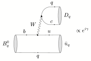
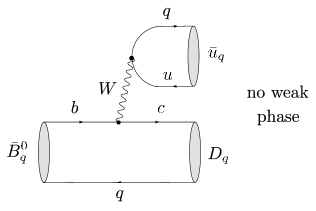
Figure 16: Feynman diagrams contributing to $B^{0}_{q}\to D_{q}\bar{u}_{q}$ and $\bar{B}^{0}_{q}\to D_{q}\bar{u}_{q}$ decays.

7.3 $B_{s}\to D_{s}^{\pm}K^{\mp}$ and $B_{d}\to D^{\pm}\pi^{\mp}$

The decays $B_{s}\to D_{s}^{\pm}K^{\mp}$ [187] and $B_{d}\to D^{\pm}\pi^{\mp}$ [188] can be treated on the same theoretical basis, and provide new strategies to determine $\gamma$ [81]. Following this paper, we write these modes, which are pure “tree” decays according to the classification of Subsection 3.2, generically as $B_{q}\to D_{q}\bar{u}_{q}$. As can be seen from the Feynman diagrams in Fig. 16, their characteristic feature is that both a $B^{0}_{q}$ and a $\bar{B}^{0}_{q}$ meson may decay into the same final state $D_{q}\bar{u}_{q}$. Consequently, as illustrated in Fig. 17, interference effects between $B^{0}_{q}$–$\bar{B}^{0}_{q}$ mixing and decay processes arise, which allow us to probe the weak phase $\phi_{q}+\gamma$ through measurements of the corresponding time-dependent decay rates.

In the case of $q=s$, i.e. $D_{s}\in\{D_{s}^{+},D_{s}^{\ast+},...\}$ and $u_{s}\in\{K^{+},K^{\ast+},...\}$, these interference effects are governed by a hadronic parameter $X_{s}e^{i\delta_{s}}\propto R_{b}\approx 0.4$, where $R_{b}\propto|V_{ub}/V_{cb}|$ is the usual UT side, and hence are large. On the other hand, for $q=d$, i.e. $D_{d}\in\{D^{+},D^{\ast+},...\}$ and $u_{d}\in\{\pi^{+},\rho^{+},...\}$, the interference effects are described by $X_{d}e^{i\delta_{d}}\propto-\lambda^{2}R_{b}\approx-0.02$, and hence are tiny. In the following, we shall only consider $B_{q}\to D_{q}\overline{u}_{q}$ modes, where at least one of the $D_{q}$, $\bar{u}_{q}$ states is a pseudoscalar meson; otherwise a complicated angular analysis has to be performed.

Figure 17: Interference effects between $B^{0}_{q}\to D_{q}\bar{u}_{q}$ and $\bar{B}^{0}_{q}\to D_{q}\bar{u}_{q}$ decays.

The time-dependent rate asymmetries of these decays take the same form as (52). It is well known that they allow a theoretically clean determination of $\phi_{q}+\gamma$, where the “conventional” approach works as follows [187, 188]: if we measure the observables $C(B_{q}\to D_{q}\bar{u}_{q})\equiv C_{q}$ and $C(B_{q}\to\bar{D}_{q}u_{q})\equiv\overline{C}_{q}$ provided by the $\cos(\Delta M_{q}t)$ pieces, we may determine the following quantities:

$$\langle C_{q}\rangle_{+}\equiv\frac{1}{2}\left[\overline{C}_{q}+C_{q}\right]=0,\quad\langle C_{q}\rangle_{-}\equiv\frac{1}{2}\left[\overline{C}_{q}-C_{q}\right]=\frac{1-X_{q}^{2}}{1+X_{q}^{2}},$$ (212)

where $\langle C_{q}\rangle_{-}$ allows us to extract $X_{q}$. However, to this end we have to resolve terms entering at the $X_{q}^{2}$ level. In the case of $q=s$, we have $X_{s}={\cal O}(R_{b})$, implying $X_{s}^{2}={\cal O}(0.16)$, so that this should actually be possible, though challenging. On the other hand, $X_{d}={\cal O}(-\lambda^{2}R_{b})$ is doubly Cabibbo-suppressed. Although it should be possible to resolve terms of ${\cal O}(X_{d})$, this will be impossible for the vanishingly small $X_{d}^{2}={\cal O}(0.0004)$ terms, so that other approaches to fix $X_{d}$ are required [188]. For the extraction of $\phi_{q}+\gamma$, the mixing-induced observables $S(B_{q}\to D_{q}\bar{u}_{q})\equiv S_{q}$ and $S(B_{q}\to\bar{D}_{q}u_{q})\equiv\overline{S}_{q}$ associated with the $\sin(\Delta M_{q}t)$ terms of the time-dependent rate asymmetry must be measured. In analogy to (212), it is convenient to introduce observable combinations $\langle S_{q}\rangle_{\pm}$. Assuming that $X_{q}$ is known, we may consider the quantities

$$s_{+} \equiv (-1)^{L}\left[\frac{1+X_{q}^{2}}{2X_{q}}\right]\langle S_{q}\rangle_{+}=+\cos\delta_{q}\sin(\phi_{q}+\gamma)$$ (213)

$$s_{-} \equiv (-1)^{L}\left[\frac{1+X_{q}^{2}}{2X_{q}}\right]\langle S_{q}\rangle_{-}=-\sin\delta_{q}\cos(\phi_{q}+\gamma),$$ (214)

which yield

$$\sin^{2}(\phi_{q}+\gamma)=\frac{1}{2}\left[(1+s_{+}^{2}-s_{-}^{2})\pm\sqrt{(1+s_{+}^{2}-s_{-}^{2})^{2}-4s_{+}^{2}}\right],$$ (215)

implying an eightfold solution for $\phi_{q}+\gamma$. If we fix the sign of $\cos\delta_{q}$ through factorization, still a fourfold discrete ambiguity is left, which is limiting the power for the search of NP significantly. Note that this assumption allows us also to fix the sign of $\sin(\phi_{q}+\gamma)$ through $\langle S_{q}\rangle_{+}$. To this end, the factor $(-1)^{L}$, where $L$ is the $D_{q}\bar{u}_{q}$ angular momentum, has to be properly taken into account. This is a crucial issue for the extraction of the sign of $\sin(\phi_{d}+\gamma)$ from $B_{d}\to D^{\ast\pm}\pi^{\mp}$ decays.

Let us now discuss new strategies to explore CP violation through $B_{q}\to D_{q}\bar{u}_{q}$ modes, following Ref. [81]. If $\Delta\Gamma_{s}$ is sizeable, the “untagged” rates introduced in (209) allow us to measure ${\cal A}_{\rm\Delta\Gamma}(B_{s}\to D_{s}\bar{u}_{s})\equiv{\cal A}_{\rm\Delta\Gamma_{s}}$ and ${\cal A}_{\rm\Delta\Gamma}(B_{s}\to\bar{D}_{s}u_{s})\equiv\overline{{\cal A}}_{\rm\Delta\Gamma_{s}}$. Introducing, in analogy to (212), observable combinations $\langle{\cal A}_{\rm\Delta\Gamma_{s}}\rangle_{\pm}$, we may derive the relations

$$\tan(\phi_{s}+\gamma)=-\left[\frac{\langle S_{s}\rangle_{+}}{\langle{\cal A}_{\rm\Delta\Gamma_{s}}\rangle_{+}}\right]=+\left[\frac{\langle{\cal A}_{\rm\Delta\Gamma_{s}}\rangle_{-}}{\langle S_{s}\rangle_{-}}\right],$$ (216)

which allow an unambiguous extraction of $\phi_{s}+\gamma$ if we fix the sign of $\cos\delta_{q}$ through factorization. Another important advantage of (216) is that we do not have to rely on ${\cal O}(X_{s}^{2})$ terms, as $\langle S_{s}\rangle_{\pm}$ and $\langle{\cal A}_{\rm\Delta\Gamma_{s}}\rangle_{\pm}$ are proportional to $X_{s}$. On the other hand, a sizeable value of $\Delta\Gamma_{s}$ is of course needed.

If we keep the hadronic quantities $X_{q}$ and $\delta_{q}$ as “unknown”, free parameters in the expressions for the $\langle S_{q}\rangle_{\pm}$, we may obtain bounds on $\phi_{q}+\gamma$ from

$$|\sin(\phi_{q}+\gamma)|\geq|\langle S_{q}\rangle_{+}|,\quad|\cos(\phi_{q}+\gamma)|\geq|\langle S_{q}\rangle_{-}|.$$ (217)

If $X_{q}$ is known, stronger constraints are implied by

$$|\sin(\phi_{q}+\gamma)|\geq|s_{+}|,\quad|\cos(\phi_{q}+\gamma)|\geq|s_{-}|.$$ (218)

Once $s_{+}$ and $s_{-}$ are known, we may of course determine $\phi_{q}+\gamma$ through the “conventional” approach, using (215). However, the bounds following from (218) provide essentially the same information and are much simpler to implement. Moreover, as discussed in detail in Ref. [81] for several examples within the SM, the bounds following from the $B_{s}$ and $B_{d}$ modes may be highly complementary, thereby providing particularly narrow, theoretically clean ranges for $\gamma$.

Let us now further exploit the complementarity between the $B_{s}^{0}\to D_{s}^{(\ast)+}K^{-}$ and $B_{d}^{0}\to D^{(\ast)+}\pi^{-}$ processes. Looking at the corresponding decay topologies, we see that these channels are related to each other through an interchange of all down and strange quarks. Consequently, applying again the $U$-spin symmetry implies $a_{s}=a_{d}$ and $\delta_{s}=\delta_{d}$, where $a_{s}\equiv X_{s}/R_{b}$ and $a_{d}\equiv-X_{d}/(\lambda^{2}R_{b})$ are the ratios of the hadronic matrix elements entering $X_{s}$ and $X_{d}$, respectively. There are various possibilities to implement these relations [81]. A particularly simple picture arises if we assume that $a_{s}=a_{d}$ and $\delta_{s}=\delta_{d}$, which yields

$$\tan\gamma=-\left[\frac{\sin\phi_{d}-S\sin\phi_{s}}{\cos\phi_{d}-S\cos\phi_{s}}\right]\stackrel{{\scriptstyle\phi_{s}=0^{\circ}}}{{=}}-\left[\frac{\sin\phi_{d}}{\cos\phi_{d}-S}\right].$$ (219)

Here we have introduced

$$S\equiv-R\left[\frac{\langle S_{d}\rangle_{+}}{\langle S_{s}\rangle_{+}}\right]$$ (220)

with

$$R\equiv\left(\frac{1-\lambda^{2}}{\lambda^{2}}\right)\left[\frac{1}{1+X_{s}^{2}}\right],$$ (221)

where $R$ can be fixed with the help of untagged $B_{s}$ rates through

$$R=\left(\frac{f_{K}}{f_{\pi}}\right)^{2}\left[\frac{\Gamma(\bar{B}^{0}_{s}\to D_{s}^{(\ast)+}\pi^{-})+\Gamma(B^{0}_{s}\to D_{s}^{(\ast)-}\pi^{+})}{\langle\Gamma(B_{s}\to D_{s}^{(\ast)+}K^{-})\rangle+\langle\Gamma(B_{s}\to D_{s}^{(\ast)-}K^{+})\rangle}\right].$$ (222)

Alternatively, we can only assume that $\delta_{s}=\delta_{d}$ or that $a_{s}=a_{d}$ [81]. An important feature of this strategy is that it allow us to extract an unambiguous value of $\gamma$, which is crucial for the search of NP; first studies for LHCb are very promising in this respect [189]. Another advantage with respect to the “conventional” approach is that $X_{q}^{2}$ terms have not to be resolved experimentally. In particular, $X_{d}$ does not have to be fixed, and $X_{s}$ may only enter through a $1+X_{s}^{2}$ correction, which can straightforwardly be determined through untagged $B_{s}$ rate measurements. In the most refined implementation of this strategy, the measurement of $X_{d}/X_{s}$ would only be interesting for the inclusion of $U$-spin-breaking corrections in $a_{d}/a_{s}$. Moreover, we may obtain interesting insights into hadron dynamics and $U$-spin breaking.

The colour-suppressed counterparts of the $B_{q}\to D_{q}\bar{u}_{q}$ modes are also interesting for the exploration of CP violation. In the case of the $B_{d}\to DK_{\rm S(L)}$, $B_{s}\to D\eta^{(^{\prime})},D\phi$, … modes, the interference effects between $B^{0}_{q}$–$\bar{B}^{0}_{q}$ mixing and decay processes are governed by $x_{f_{s}}e^{i\delta_{f_{s}}}\propto R_{b}$. If we consider the CP eigenstates $D_{\pm}$ of the neutral $D$-meson system, we obtain additional interference effects at the amplitude level, which involve $\gamma$, and may introduce the following “untagged” rate asymmetry [84]:

$$\Gamma_{+-}^{f_{s}}\equiv\frac{\langle\Gamma(B_{q}\to D_{+}f_{s})\rangle-\langle\Gamma(B_{q}\to D_{-}f_{s})\rangle}{\langle\Gamma(B_{q}\to D_{+}f_{s})\rangle+\langle\Gamma(B_{q}\to D_{-}f_{s})\rangle},$$ (223)

which allows us to constrain $\gamma$ through the relation

$$|\cos\gamma|\geq|\Gamma_{+-}^{f_{s}}|.$$ (224)

Moreover, if we complement $\Gamma_{+-}^{f_{s}}$ with

$$\langle S_{f_{s}}\rangle_{\pm}\equiv\frac{1}{2}\left[S_{+}^{f_{s}}\pm S_{-}^{f_{s}}\right],$$ (225)

where $S_{\pm}^{f_{s}}\equiv{\cal A}_{\rm CP}^{\rm mix}(B_{q}\to D_{\pm}f_{s})$, we may derive the following simple but exact relation:

$$\tan\gamma\cos\phi_{q}=\left[\frac{\eta_{f_{s}}\langle S_{f_{s}}\rangle_{+}}{\Gamma_{+-}^{f_{s}}}\right]+\left[\eta_{f_{s}}\langle S_{f_{s}}\rangle_{-}-\sin\phi_{q}\right],$$ (226)

with $\eta_{f_{s}}\equiv(-1)^{L}\eta_{\rm CP}^{f_{s}}$. This expression allows a conceptually simple, theoretically clean and essentially unambiguous determination of $\gamma$ [84]. Since the interference effects are governed by the tiny parameter $x_{f_{d}}e^{i\delta_{f_{d}}}\propto-\lambda^{2}R_{b}$ in the case of $B_{s}\to D_{\pm}K_{\rm S(L)}$, $B_{d}\to D_{\pm}\pi^{0},D_{\pm}\rho^{0},...$, these modes are not as interesting for the extraction of $\gamma$. However, they provide the relation

$$\eta_{f_{d}}\langle S_{f_{d}}\rangle_{-}=\sin\phi_{q}+{\cal O}(x_{f_{d}}^{2})=\sin\phi_{q}+{\cal O}(4\times 10^{-4}),$$ (227)

allowing very interesting determinations of $\phi_{q}$ with theoretical accuracies one order of magnitude higher than those of the conventional $B^{0}_{d}\to J/\psi K_{\rm S}$ and $B^{0}_{s}\to J/\psi\phi$ approaches [84]. As we pointed out in Subsection 4.1, these measurements would be very interesting in view of the new world average of $(\sin 2\beta)_{\psi K_{\rm S}}$.

7.4 $B^{0}_{s}\to K^{+}K^{-}$ and $B^{0}_{d}\to\pi^{+}\pi^{-}$

The decay $B^{0}_{s}\to K^{+}K^{-}$ is a $\bar{b}\to\bar{s}$ transition, and involves tree and penguin amplitudes, as the $B^{0}_{d}\to\pi^{+}\pi^{-}$ mode [100]. However, because of the different CKM structure, the latter topologies play actually the dominant rôle in the $B^{0}_{s}\to K^{+}K^{-}$ channel. In analogy to (98), we may write

$$A(B_{s}^{0}\to K^{+}K^{-})=\sqrt{\epsilon}\,\,{\cal C}^{\prime}\left[e^{i\gamma}+\frac{1}{\epsilon}\,d^{\prime}e^{i\theta^{\prime}}\right],$$ (228)

where $\epsilon$ was introduced in (115), and the CP-conserving hadronic parameters ${\cal C}^{\prime}$ and $d^{\prime}e^{i\theta^{\prime}}$ correspond to ${\cal C}$ and $de^{i\theta}$, respectively. The corresponding observables take then the following generic form:

$${\cal A}_{\rm CP}^{\rm dir}(B_{s}\to K^{+}K^{-}) = G_{1}^{\prime}(d^{\prime},\theta^{\prime};\gamma)$$ (229)

$${\cal A}_{\rm CP}^{\rm mix}(B_{s}\to K^{+}K^{-}) = G_{2}^{\prime}(d^{\prime},\theta^{\prime};\gamma,\phi_{s}),$$ (230)

in analogy to the expressions for the CP-violating $B^{0}_{d}\to\pi^{+}\pi^{-}$ asymmetries in (103) and (104). Since $\phi_{d}=(43.4\pm 2.5)^{\circ}$ is already known (see Subsection 4.1) and $\phi_{s}$ is negligibly small in the SM – or can be determined through $B^{0}_{s}\to J/\psi\phi$ should CP-violating NP contributions to $B^{0}_{s}$–$\bar{B}^{0}_{s}$ mixing make it sizeable – we may convert the measured values of ${\cal A}_{\rm CP}^{\rm dir}(B_{d}\to\pi^{+}\pi^{-})$, ${\cal A}_{\rm CP}^{\rm mix}(B_{d}\to\pi^{+}\pi^{-})$ and ${\cal A}_{\rm CP}^{\rm dir}(B_{s}\to K^{+}K^{-})$, ${\cal A}_{\rm CP}^{\rm mix}(B_{s}\to K^{+}K^{-})$ into theoretically clean contours in the $\gamma$–$d$ and $\gamma$–$d^{\prime}$ planes, respectively. In Fig. 18, we show these contours for an example, which corresponds to the central values of (111) and (112) with the hadronic parameters $(d,\theta)$ in (128).

As can be seen in Fig. 11, the decay $B^{0}_{d}\to\pi^{+}\pi^{-}$ is actually related to $B^{0}_{s}\to K^{+}K^{-}$ through the interchange of all down and strange quarks. Consequently, each decay topology contributing to $B^{0}_{d}\to\pi^{+}\pi^{-}$ has a counterpart in $B^{0}_{s}\to K^{+}K^{-}$, and the corresponding hadronic parameters can be related to each other with the help of the $U$-spin flavour symmetry of strong interactions, implying the following relations [100]:

$$d^{\prime}=d,\quad\theta^{\prime}=\theta.$$ (231)

Applying the former, we may extract $\gamma$ and $d$ through the intersections of the theoretically clean $\gamma$–$d$ and $\gamma$–$d^{\prime}$ contours. As discussed in Ref. [100], it is also possible to resolve straightforwardly the twofold ambiguity for $(\gamma,d)$ arising in Fig. 18, thereby leaving us with the “true” solution of $\gamma=74^{\circ}$ in this example. Moreover, we may determine $\theta$ and $\theta^{\prime}$, which allow an interesting internal consistency check of the second $U$-spin relation in (231). An alternative avenue is provided if we eliminate $d$ and $d^{\prime}$ through the CP-violating $B_{d}\to\pi^{+}\pi^{-}$ and $B_{s}\to K^{+}K^{-}$ observables, respectively, and extract then these parameters and $\gamma$ through the $U$-spin relation $\theta^{\prime}=\theta$.

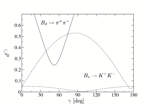
Figure 18: The contours in the $\gamma$–$d^{(^{\prime})}$ plane for an example with $d=d^{\prime}=0.52$, $\theta=\theta^{\prime}=146^{\circ}$, $\phi_{d}=43.4^{\circ}$, $\phi_{s}=-2^{\circ}$, $\gamma=74^{\circ}$, which corresponds to the CP asymmetries ${\cal A}_{\rm CP}^{\rm dir}(B_{d}\to\pi^{+}\pi^{-})=-0.37$ and ${\cal A}_{\rm CP}^{\rm mix}(B_{d}\to\pi^{+}\pi^{-})=+0.50$ (see Subsections 4.3 and 5.2), as well as ${\cal A}_{\rm CP}^{\rm dir}(B_{s}\to K^{+}K^{-})=+0.12$ and ${\cal A}_{\rm CP}^{\rm mix}(B_{s}\to K^{+}K^{-})=-0.19$.

This strategy is very promising from an experimental point of view for LHCb, where an accuracy for $\gamma$ of a few degrees can be achieved [77, 171, 190]. As far as possible $U$-spin-breaking corrections to $d^{\prime}=d$ are concerned, they enter the determination of $\gamma$ through a relative shift of the $\gamma$–$d$ and $\gamma$–$d^{\prime}$ contours; their impact on the extracted value of $\gamma$ therefore depends on the form of these curves, which is fixed through the measured observables. In the examples discussed in Refs. [49, 100], as well as in the one shown in Fig. 18, the extracted value of $\gamma$ would be very stable under such effects. Let us also note that the $U$-spin relations in (231) are particularly robust since they involve only ratios of hadronic amplitudes, where all $SU(3)$-breaking decay constants and form factors cancel in factorization and also chirally enhanced terms would not lead to $U$-spin-breaking corrections [100]. On the other hand, the ratio $|{\cal C}^{\prime}/{\cal C}|$, which equals 1 in the strict $U$-spin limit and enters the $U$-spin relation

$$\frac{{\cal A}_{\rm CP}^{\rm mix}(B_{s}\to K^{+}K^{-})}{{\cal A}_{\rm CP}^{\rm dir}(B_{d}\to\pi^{+}\pi^{-})}=-\left|\frac{{\cal C}^{\prime}}{{\cal C}}\right|^{2}\left[\frac{\mbox{BR}(B_{d}\to\pi^{+}\pi^{-})}{\mbox{BR}(B_{s}\to K^{+}K^{-})}\right]\frac{\tau_{B_{s}}}{\tau_{B_{d}}},$$ (232)

is affected by $U$-spin-breaking effects within factorization. An estimate of the corresponding form factors was recently performed in Ref. [191] with the help of QCD sum rules, which is an important ingredient for a SM prediction of the CP-averaged $B_{s}\to K^{+}K^{-}$ branching ratio [39, 139], yielding a value in accordance with the first results reported by the CDF collaboration [192]. For other recent analyses of the $B_{s}\to K^{+}K^{-}$ decay, see Refs. [193, 194]

In addition to the $B_{s}\to K^{+}K^{-}$, $B_{d}\to\pi^{+}\pi^{-}$ and $B_{s}\to D_{s}^{\pm}K^{\mp}$, $B_{d}\to D^{\pm}\pi^{\mp}$ strategies discussed above, also other $U$-spin methods for the extraction of $\gamma$ were proposed, using $B_{s(d)}\to J/\psi K_{\rm S}$ or $B_{d(s)}\to D_{d(s)}^{+}D_{d(s)}^{-}$ [72], $B_{d(s)}\to K^{0(*)}\bar{K}^{0(*)}$ [49, 184], $B_{(s)}\to\pi K$ [195], or $B_{s(d)}\to J/\psi\eta$ modes [196]. In a very recent paper [197], also two-body decays of charged $B$ mesons were considered.

     

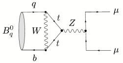
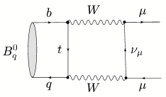
Figure 19: Feynman diagrams contributing to $B^{0}_{q}\to\mu^{+}\mu^{-}$ ($q\in\{s,d\}$).

7.5 $B^{0}_{s}\to\mu^{+}\mu^{-}$ and $B^{0}_{d}\to\mu^{+}\mu^{-}$

Let us finally have a closer look at the rare decay $B^{0}_{s}\to\mu^{+}\mu^{-}$, which we encountered already briefly in Subsection 5.4. As can be seen in Fig. 19, this decay and its $B_{d}$-meson counterpart $B^{0}_{d}\to\mu^{+}\mu^{-}$ originate from $Z^{0}$-penguin and box diagrams in the SM. The corresponding low-energy effective Hamiltonian is given as follows [32]:

$${\cal H}_{\rm eff}=-\frac{G_{\rm F}}{\sqrt{2}}\left[\frac{\alpha}{2\pi\sin^{2}\Theta_{\rm W}}\right]V_{tb}^{\ast}V_{tq}\eta_{Y}Y_{0}(x_{t})(\bar{b}q)_{\rm V-A}(\bar{\mu}\mu)_{\rm V-A}\,+\,{\rm h.c.},$$ (233)

where $\alpha$ denotes the QED coupling and $\Theta_{\rm W}$ is the Weinberg angle. The short-distance physics is described by $Y(x_{t})\equiv\eta_{Y}Y_{0}(x_{t})$, where $\eta_{Y}=1.012$ is a perturbative QCD correction [198]–[200], and the Inami–Lim function $Y_{0}(x_{t})$ describes the top-quark mass dependence. We observe that only the matrix element $\langle 0|(\bar{b}q)_{\rm V-A}|B^{0}_{q}\rangle$ is required. Since here the vector-current piece vanishes, as the $B^{0}_{q}$ is a pseudoscalar meson, this matrix element is simply given by the decay constant $f_{B_{q}}$, which is defined in analogy to (116). Consequently, we arrive at a very favourable situation with respect to the hadronic matrix elements. Since, moreover, NLO QCD corrections were calculated, and long-distance contributions are expected to play a negligible rôle [198], the $B^{0}_{q}\to\mu^{+}\mu^{-}$ modes belong to the cleanest rare $B$ decays. The SM branching ratios can then be written in the following compact form [201]:

$$\mbox{BR}(B_{s}\to\mu^{+}\mu^{-})=4.1\times 10^{-9}$$ (234)

$$\qquad\qquad\times\left[\frac{f_{B_{s}}}{0.24\,\mbox{GeV}}\right]^{2}\left[\frac{|V_{ts}|}{0.040}\right]^{2}\left[\frac{\tau_{B_{s}}}{1.5\,\mbox{ps}}\right]\left[\frac{m_{t}}{167\,\mbox{GeV}}\right]^{3.12}$$

$$\mbox{BR}(B_{d}\to\mu^{+}\mu^{-})=1.1\times 10^{-10}$$ (235)

$$\qquad\qquad\times\left[\frac{f_{B_{d}}}{0.20\,\mbox{GeV}}\right]^{2}\left[\frac{|V_{td}|}{0.008}\right]^{2}\left[\frac{\tau_{B_{d}}}{1.5\,\mbox{ps}}\right]\left[\frac{m_{t}}{167\,\mbox{GeV}}\right]^{3.12}.$$

The most recent upper bounds (90% C.L.) from CDF read as follows [202]:

$$\mbox{BR}(B_{s}\to\mu^{+}\mu^{-})<1.5\times 10^{-7},\quad\mbox{BR}(B_{d}\to\mu^{+}\mu^{-})<3.9\times 10^{-8},$$ (236)

while the D0 collaboration finds the following (95% C.L.) upper limit [203]:

$$\mbox{BR}(B_{s}\to\mu^{+}\mu^{-})<3.7\times 10^{-7}.$$ (237)

Using again relation (203), we find that the measurement of the ratio

$$\frac{\mbox{BR}(B_{d}\to\mu^{+}\mu^{-})}{\mbox{BR}(B_{s}\to\mu^{+}\mu^{-})}=\left[\frac{\tau_{B_{d}}}{\tau_{B_{s}}}\right]\left[\frac{M_{B_{d}}}{M_{B_{s}}}\right]\left[\frac{f_{B_{d}}}{f_{B_{s}}}\right]^{2}\left|\frac{V_{td}}{V_{ts}}\right|^{2}$$ (238)

would allow an extraction of the UT side $R_{t}$. Since the short-distance function $Y$ cancels, this determination does not only work in the SM, but also in the NP scenarios with MFV [67]. This strategy is complementary to that offered by (204), using $\Delta M_{d}/\Delta M_{s}$. If we look at (204) and (238), we see that these expressions imply another relation [204]:

$$\frac{\mbox{BR}(B_{s}\to\mu^{+}\mu^{-})}{\mbox{BR}(B_{d}\to\mu^{+}\mu^{-})}=\left[\frac{\tau_{B_{s}}}{\tau_{B_{d}}}\right]\left[\frac{\hat{B}_{B_{d}}}{\hat{B}_{B_{s}}}\right]\left[\frac{\Delta M_{s}}{\Delta M_{d}}\right],$$ (239)

which holds again in the context of MFV models, including the SM. Here the advantage is that the dependence on $(f_{B_{d}}/f_{B_{s}})^{2}$ cancels. Moreover, we may also use the (future) experimental data for $\Delta M_{(s)d}$ to reduce the hadronic uncertainties of the SM predictions of the $B_{q}\to\mu^{+}\mu^{-}$ branching ratios [204]:

$$\mbox{BR}(B_{s}\to\mu^{+}\mu^{-}) = (3.42\pm 0.53)\times\left[\frac{\Delta M_{s}}{18.0\,{\rm ps}^{-1}}\right]\times 10^{-9}$$ (240)

$$\mbox{BR}(B_{d}\to\mu^{+}\mu^{-}) = (1.00\pm 0.14)\times 10^{-10}.$$ (241)

The current experimental upper bounds in (236) and (237) are still about two orders of magnitude away from these numbers. Consequently, should the $B_{q}\to\mu^{+}\mu^{-}$ decays be governed by their SM contributions, we could only hope to observe them at the LHC [77]. On the other hand, since the $B_{q}\to\mu^{+}\mu^{-}$ transitions originate from FCNC processes, they are sensitive probes of NP. In particular, the branching ratios may be dramatically enhanced in specific NP (SUSY) scenarios, as was recently reviewed in Ref. [48]. Should this actually be the case, these decays may already be seen at run II of the Tevatron, and the $e^{+}e^{-}$ $B$ factories could observe $B_{d}\to\mu^{+}\mu^{-}$. Let us finally emphasize that the experimental bounds on $B_{s}\to\mu^{+}\mu^{-}$ can also be converted into bounds on NP parameters in specific scenarios. In the context of the constrained minimal supersymmetric extension of the SM (CMSSM) with universal scalar masses, such constraints were recently critically discussed by the authors of Ref. [205].

8 Conclusions and Outlook

CP violation is now well established in the $B$-meson system, thereby complementing the neutral $K$-meson system, where this phenomenon was discovered more than 40 years ago. The data of the $e^{+}e^{-}$ $B$ factories have provided valuable insights into the physics of strong and weak interactions. Concerning the former aspect, which is sometimes only considered as a by-product, the data give us important evidence for large non-factorizable effects in non-leptonic $B$-decays, so that the challenge for a reliable theoretical description within dynamical QCD approaches remains, despite interesting recent progress. As far as the latter aspect is concerned, the description of CP violation through the KM mechanism has successfully passed its first experimental tests, in particular through the comparison between the measurement of $\sin 2\beta$ with the help of $B^{0}_{d}\to J/\psi K_{\rm S}$ and the CKM fits. However, the most recent average for $(\sin 2\beta)_{\psi K_{\rm S}}$ is now somewhat on the lower side, and there are a couple of puzzles in the $B$-factory data. It will be very interesting to monitor these effects, which could be first hints for physics beyond the SM, as the data improve. Moreover, it is crucial to refine the corresponding theoretical analyses further, to have a critical look at the underlying working assumptions and to check them through independent tests, and to explore correlations with other flavour probes.

Despite this impressive progress, there are still regions of the $B$-physics landscape left that are essentially unexplored. For instance, $b\to d$ penguin processes are now entering the stage, since lower bounds for the corresponding branching ratios that can be derived in the SM turn out to be very close to the corresponding experimental upper limits. Indeed, we have now evidence for the $B_{d}\to K^{0}\bar{K}^{0}$ and $B^{\pm}\to K^{\pm}K$ channels, and the first signals for the radiative $B\to\rho\gamma$ transitions were recently reported, representing one of the hot topics of this summer. These modes have now to be explored in much more detail, and several other decays are waiting to be observed.

Moreover, also the $B_{s}$-meson system, which cannot be studied with the BaBar and Belle experiments, is still essentially unexplored. The accurate measurement of the mass difference $\Delta M_{s}$ is a key element for the testing of the quark-flavour sector of the SM, and the width difference $\Delta\Gamma_{s}$ may be sizeable, thereby offering studies with “untagged” $B_{s}$ decay rates. Moreover, the $B_{s}$-meson system provides sensitive probes to search for CP-violating NP contributions to $B^{0}_{s}$–$\bar{B}^{0}_{s}$ mixing, allows several determinations the angle $\gamma$ of the UT in an essentially unambiguous way, and offers further tests of the SM through strongly suppressed rare decays. After new results from run II of the Tevatron, the promising physics potential of the $B_{s}$-meson system can be fully exploited at the LHC, in particular by the LHCb experiment.

These studies can nicely be complemented through the kaon system, which governed the stage of CP violation for more than 35 years. The future lies now on rare decays, in particular on the $K^{+}\to\pi^{+}\nu\bar{\nu}$ and $K_{\rm L}\to\pi^{0}\nu\bar{\nu}$ modes; there is a new proposal to measure the former channel at the CERN SPS, and efforts to explore the latter at KEK/J-PARC in Japan. Furthermore, flavour physics offers several other exciting topics. Important examples are top-quark physics, the $D$-meson system, the anomalous magnetic moment of the muon, electric dipole moments and the flavour violation in the charged lepton and neutrino sectors.

The established neutrino oscillations as well as the evidence for dark matter and the baryon asymmetry of the Universe tell us that the SM is incomplete, and specific extensions contain usually also new sources of flavour and CP violation, which may manifest themselves at the flavour factories. Fortunately, the LHC is expected to go into operation in the autumn of 2007. This new accelerator will provide insights into electroweak symmetry breaking and, hopefully, also give us direct evidence for physics beyond the SM through the production and subsequent decays of NP particles in the ATLAS and CMS detectors. It is obvious that there should be a very fruitful interplay between these “direct” studies of NP, and the “indirect” information provided by flavour physics [206]. I have no doubt that an exciting future is ahead of us!

References

References

- [1] J.H. Christenson et al., Phys. Rev. Lett. 13, 138 (1964).
-
[2]
V. Fanti et al. [NA48 Collaboration],
Phys. Lett. B465, 335 (1999);
A. Alavi-Harati et al. [KTeV Collaboration], Phys. Rev. Lett. 83, 22 (1999). - [3] J.R. Batley et al. [NA48 Collaboration], Phys. Lett. B544, 97 (2002).
- [4] A. Alavi-Harati et al. [KTeV Collaboration], Phys. Rev. D67, 012005 (2003).
-
[5]
B. Aubert et al. [BaBar Collaboration],
Phys. Rev. Lett. 87, 091801 (2001);
K. Abe et al. [Belle Collaboration], Phys. Rev. Lett. 87, 091802 (2001). -
[6]
B. Aubert et al. [BaBar Collaboration],
Phys. Rev. Lett. 93, 131801 (2004);
Y. Chao et al. [Belle Collaboration], Phys. Rev. Lett. 93, 191802 (2004). - [7] A.D. Sakharov, JETP Lett. 5, 24 (1967).
-
[8]
V.A. Rubakov, M.E. Shaposhnikov,
Usp. Fiz. Nauk 166, 493 (1996);
Phys. Usp. 39, 461 (1996);
A. Riotto and M. Trodden, Annu. Rev. Nucl. Part. Sci. 49, 35 (1999). - [9] For a recent review, see W. Buchmüller, R.D. Peccei and T. Yanagida, hep-ph/0502169.
- [10] N. Cabibbo, Phys. Rev. Lett. 10, 531 (1963).
- [11] M. Kobayashi and T. Maskawa, Prog. Theor. Phys. 49, 652 (1973).
- [12] M. Battaglia et al., CERN 2003-002-corr, The CKM matrix and the unitarity triangle (CERN, Geneva, 2003) [hep-ph/0304132].
- [13] For a recent review, see A.J. Buras and M. Jamin, JHEP 0401, 048 (2004).
- [14] L. Wolfenstein, Phys. Rev. Lett. 13, 562 (1964).
- [15] G. Branco, L. Lavoura and J. Silva, CP Violation, International Series of Monographs on Physics 103, Oxford Science Publications (Clarendon Press, Oxford, 1999).
- [16] I.I. Bigi and A. I. Sanda, CP Violation, Cambridge Monographs on Particle Physics, Nuclear Physics and Cosmology (Cambridge University Press, Cambridge, 2000).
- [17] K. Kleinknecht, Springer Tracts in Modern Physics, Vol. 195 (2004).
- [18] Y. Nir, hep-ph/0510413.
- [19] M. Gronau, hep-ph/0510153.
- [20] A.J. Buras, hep-ph/0505175.
- [21] A. Ali, Int. J. Mod. Phys. A20, 5080 (2005).
- [22] S.L. Glashow, J. Iliopoulos and L. Maiani, Phys. Rev. D2, 1285 (1970).
- [23] S. Eidelman et al. [Particle Data Group], Phys. Lett. B592, 1 (2004).
- [24] L. Wolfenstein, Phys. Rev. Lett. 51, 1945 (1983).
- [25] A.J. Buras, M.E. Lautenbacher and G. Ostermaier, Phys. Rev D50, 3433 (1994).
- [26] J. Charles et al. [CKMfitter Group], Eur. Phys. J. C 41, 1 (2005); for the most recent updates, see http://ckmfitter.in2p3.fr/.
- [27] M. Bona et al. [UTfit Collaboration], JHEP 0507, 028 (2005); for the most recent updates, see http://utfit.roma1.infn.it/.
- [28] T. Inami and C.S. Lim, Prog. Theor. Phys. 65, 297 [E: 65, 1772] (1981).
- [29] S. Laplace, Z. Ligeti, Y. Nir and G. Perez, Phys. Rev. D65, 094040 (2002).
-
[30]
M. Beneke, G. Buchalla, A. Lenz and U. Nierste,
Phys. Lett. B576, 173 (2003);
M. Ciuchini, E. Franco, V. Lubicz, F. Mescia and C. Tarantino, JHEP 0308, 031 (2003). - [31] Heavy Flavour Averaging Group: http://www.slac.stanford.edu/xorg/hfag/.
-
[32]
G. Buchalla, A.J. Buras and M.E. Lautenbacher,
Rev. Mod. Phys. 68, 1125 (1996);
A.J. Buras, hep-ph/9806471. -
[33]
A.J. Buras and J.-M. Gérard,
Nucl. Phys. B264, 371 (1986);
A.J. Buras, J.-M. Gérard and R. Rückl, Nucl. Phys. B268, 16 (1986). - [34] J.D. Bjorken, Nucl. Phys. (Proc. Suppl.) B11, 325 (1989); M. Dugan and B. Grinstein, Phys. Lett. B255, 583 (1991); H.D. Politzer and M.B. Wise, Phys. Lett. B257, 399 (1991).
- [35] M. Beneke, G. Buchalla, M. Neubert and C. Sachrajda, Phys. Rev. Lett. 83, 1914 (1999); Nucl. Phys. B591, 313 (2000); Nucl. Phys. B606, 245 (2001).
- [36] H.-n. Li and H.L. Yu, Phys. Rev. D53, 2480 (1996); Y.Y. Keum, H.-n. Li and A.I. Sanda, Phys. Lett. B504, 6 (2001); Y.Y. Keum and H.-n. Li, Phys. Rev. D63, 074006 (2001).
- [37] C.W. Bauer, D. Pirjol and I.W. Stewart, Phys. Rev. Lett. 87, 201806 (2001), Phys. Rev. D65, 054022 (2002); C.W. Bauer, S. Fleming, D. Pirjol, I.Z. Rothstein and I.W. Stewart, Phys. Rev. D66, 014017 (2002); C.W. Bauer, B. Grinstein, D. Pirjol and I.W. Stewart, Phys. Rev. D67, 014010 (2003).
-
[38]
A. Khodjamirian,
Nucl. Phys. B605, 558 (2001);
A. Khodjamirian, T. Mannel and B. Melic, Phys. Lett. B571, 75 (2003). -
[39]
A.J. Buras, R. Fleischer, S. Recksiegel and F. Schwab,
Phys. Rev. Lett. 92, 101804 (2004);
Nucl. Phys. B697, 133 (2004). - [40] A. Ali, E. Lunghi and A.Y. Parkhomenko, Eur. Phys. J. C36, 183 (2004).
- [41] C.W. Chiang, M. Gronau, J.L. Rosner and D.A. Suprun, Phys. Rev. D70, 034020 (2004).
- [42] For detailed discussions, see, for instance, M. Dine, hep-ph/0011376; R.D. Peccei, hep-ph/9807514.
- [43] M. Gronau and D. Wyler, Phys. Lett. B265, 172 (1991).
- [44] D. Atwood, I. Dunietz, A. Soni, Phys. Rev. Lett. 78, 3257 (1997); Phys. Rev. D63, 036005 (2001).
- [45] R. Fleischer and D. Wyler, Phys. Rev. D62, 057503 (2000).
-
[46]
M. Gronau, J.L. Rosner and D. London,
Phys. Rev. Lett. 73, 21 (1994);
M. Gronau, O.F. Hernandez, D. London and J.L. Rosner, Phys. Rev. D50, 4529 (1994). -
[47]
A.B. Carter and A.I. Sanda,
Phys. Rev. Lett. 45, 952 (1980);
Phys. Rev. D23, 1567 (1981);
I.I. Bigi and A.I. Sanda, Nucl. Phys. B193, 85 (1981). - [48] A.J. Buras, hep-ph/0402191.
- [49] R. Fleischer, Phys. Rep. 370, 537 (2002).
- [50] For reviews, see, for instance, A. Ali, hep-ph/0412128; G. Isidori, AIP Conf. Proc. 722, 181 (2004); M. Misiak, Acta Phys. Polon. B34, 4397 (2003).
- [51] R. Fleischer and T. Mannel, Phys. Lett. B506, 311 (2001).
- [52] R. Fleischer, G. Isidori and J. Matias, JHEP 0305, 053 (2003).
- [53] R. Fleischer and T. Mannel, Phys. Lett. B511, 240 (2001).
- [54] T. Goto et al., Phys. Rev. D70, 035012 (2004).
- [55] S. Jäger and U. Nierste, Eur. Phys. J. C33, S256 (2004).
- [56] M. Ciuchini, E. Franco, A. Masiero and L. Silvestrini, eConf C0304052, WG307 (2003) [J. Korean Phys. Soc. 45, S223 (2004)].
- [57] P. Ball, S. Khalil and E. Kou, Phys. Rev. D69, 115011 (2004).
- [58] P. Ko, J. Korean Phys. Soc. 45, S410 (2004).
- [59] E. Gabrielli, K. Huitu and S. Khalil, hep-ph/0504168.
-
[60]
P. Ball, J.M. Frere and J. Matias,
Nucl. Phys. B572, 3 (2000);
P. Ball and R. Fleischer, Phys. Lett. B475, 111 (2000). -
[61]
A.J. Buras, M. Spranger and A. Weiler,
Nucl. Phys. B660, 225 (2003);
A.J. Buras, A. Poschenrieder, M. Spranger and A. Weiler, Nucl. Phys. B678, 455 (2004);
K. Agashe, G. Perez and A. Soni, Phys. Rev. Lett. 93, 201804 (2004), Phys. Rev. D71, 016002 (2005). - [62] V. Barger, C.W. Chiang, J. Jiang and P. Langacker, Phys. Lett. B596, 229 (2004).
-
[63]
S.R. Choudhury, N. Gaur, A. Goyal and N. Mahajan,
Phys. Lett. B601, 164 (2004);
A.J. Buras, A. Poschenrieder and S. Uhlig, Nucl. Phys. B716, 173 (2005). - [64] W.S. Hou, M. Nagashima and A. Soddu, Phys. Rev. Lett. 95, 141601 (2005).
- [65] A.J. Buras, P. Gambino, M. Gorbahn, S. Jäger and L. Silvestrini, Phys. Lett. B500, 161 (2001).
- [66] G. D’Ambrosio, G.F. Giudice, G. Isidori and A. Strumia, Nucl. Phys. B645, 155 (2002).
- [67] A.J. Buras, Acta Phys. Polon. B34, 5615 (2003).
- [68] K. Agashe, M. Papucci, G. Perez and D. Pirjol, hep-ph/0509117.
- [69] For a review, see A.A. Petrov, Nucl. Phys. (Proc. Suppl.) B142, 333 (2005).
- [70] For a review, see M. Pospelov and A. Ritz, Annals Phys. 318, 119 (2005).
- [71] For a recent analysis, see P.H. Chankowski, J.R. Ellis, S. Pokorski, M. Raidal and K. Turzynski, Nucl. Phys. B690, 279 (2004).
- [72] R. Fleischer, Eur. Phys. J. C10, 299 (1999).
- [73] B. Aubert et al. [BaBar Collaboration], Phys. Rev. Lett. 94, 161803 (2005).
- [74] K. Abe et al. [Belle Collaboration], BELLE-CONF-0569 [hep-ex/0507037].
- [75] H. Boos, T. Mannel and J. Reuter, Phys. Rev. D70, 036006 (2004).
- [76] M. Ciuchini, M. Pierini and L. Silvestrini, hep-ph/0507290.
- [77] P. Ball et al., hep-ph/0003238, in CERN Report on Standard Model physics (and more) at the LHC (CERN, Geneva, 2000), p. 305.
- [78] R. Fleischer, Int. J. Mod. Phys. A12, 2459 (1997).
- [79] R. Fleischer and J. Matias, Phys. Rev. D66, 054009 (2002).
- [80] B. Aubert et al. [BaBar Collaboration], Phys. Rev. D71, 032005 (2005).
- [81] R. Fleischer, Nucl. Phys. B671, 459 (2003).
- [82] A. Bondar, T. Gershon and P. Krokovny, Phys. Lett. B624, 1 (2005).
- [83] Tim Gershon, private communication.
- [84] R. Fleischer, Phys. Lett. B562 (2003) 234; Nucl. Phys. B659 (2003) 321.
-
[85]
D. London and R.D. Peccei,
Phys. Lett. B223, 257 (1989);
N.G. Deshpande and J. Trampetic, Phys. Rev. D41, 895 and 2926 (1990);
J.-M. Gérard and W.-S. Hou, Phys. Rev. D43, 2909; Phys. Lett. B253, 478 (1991). - [86] R. Fleischer, Z. Phys. C62, 81 (1994).
- [87] N.G. Deshpande and X.-G. He, Phys. Lett. B336, 471 (1994).
- [88] Y. Grossman and M.P. Worah, Phys. Lett. B395, 241 (1997).
- [89] V. Barger, C.W. Chiang, P. Langacker and H.S. Lee, Phys. Lett. B598, 218 (2004).
- [90] XXI International Symposium on Lepton and Photon Interactions at High Energies (LP ’03), 11–16 August 2003, Fermilab, Batavia, IL, USA, http://conferences.fnal.gov/lp2003/.
- [91] 32nd International Conference on High-Energy Physics (ICHEP ’04), 16–22 August 2004, Beijing, China, http://ichep04.ihep.ac.cn/.
- [92] XXII International Symposium on Lepton and Photon Interactions at High Energies (LP ’05), 30 June – 5 July 2005, Uppsala, Sweden, http://lp2005.tsl.uu.se/ lp2005/.
- [93] B. Aubert et al. [BaBar Collaboration], Phys. Rev. D71, 091102 (2005).
- [94] K. Abe et al. [Belle Collaboration], BELLE-CONF-0569 [hep-ex/0507037].
- [95] R. Fleischer, Phys. Lett. B365, 399 (1996).
- [96] D. London and A. Soni, Phys. Lett. B407, 61 (1997).
- [97] M. Gronau, Y. Grossman and J.L. Rosner, Phys. Lett. B579, 331 (2004).
- [98] M. Beneke, Phys. Lett. 620, 143 (2005).
-
[99]
A.J. Buras, R. Fleischer, S. Recksiegel and F. Schwab,
hep-ph/0512032,
to appear in Eur. Phys. J. C. - [100] R. Fleischer, Phys. Lett. B459, 306 (1999).
- [101] M. Gronau and D. London, Phys. Rev. Lett. 65, 3381 (1990).
- [102] J.P. Silva and L. Wolfenstein, Phys. Rev. D49, 1151 (1994).
- [103] R. Fleischer and T. Mannel, Phys. Lett. B397, 269 (1997).
- [104] Y. Grossman and H.R. Quinn, Phys. Rev. D58, 017504 (1998).
- [105] J. Charles, Phys. Rev. D59, 054007 (1999).
- [106] M. Gronau, D. London, N. Sinha and R. Sinha, Phys. Lett. B514, 315 (2001).
- [107] B. Aubert et al. [BaBar Collaboration], Phys. Rev. Lett. 95, 151803 (2005).
- [108] K. Abe et al. [Belle Collaboration], BELLE-CONF-0501 [hep-ex/0502035].
- [109] R. Fleischer, Eur. Phys. J. C16, 87 (2000).
- [110] R. Fleischer and J. Matias, Phys. Rev. D66, 054009 (2002).
- [111] C.W. Bauer, I.Z. Rothstein and I.W. Stewart, Phys. Rev. Lett. 94, 231802 (2005).
- [112] C.W. Bauer, I.Z. Rothstein and I.W. Stewart, hep-ph/0510241.
- [113] B. Aubert et al. [BaBar Collaboration], BABAR-CONF-05-018 [hep-ex/0507101].
- [114] K. Abe et al. [Belle Collaboration], BELLE-CONF-0476 [hep-ex/0411049].
- [115] Y. Grossman, Y. Nir and M.P. Worah, Phys. Lett. B407, 307 (1997).
-
[116]
T. Goto, N. Kitazawa, Y. Okada and M. Tanaka,
Phys. Rev. D53, 6662 (1996);
A.G. Cohen, D.B. Kaplan, F. Lepeintre and A.E. Nelson, Phys. Rev. Lett. 78, 2300 (1997);
G. Barenboim, G. Eyal and Y. Nir, Phys. Rev. Lett. 83, 4486 (1999). - [117] M. Bona et al. [UTfit Collaboration], hep-ph/0509219.
- [118] B. Aubert et al. [BaBar Collaboration], Phys. Rev. Lett. 95, 041805 (2005).
- [119] K. Abe et al. [Belle Collaboration] BELLE-CONF-0545 [hep-ex/0507039].
- [120] R. Fleischer and T. Mannel, hep-ph/9706261.
- [121] Y. Grossman, M. Neubert and A.L. Kagan, JHEP 9910, 029 (1999).
- [122] A.J. Buras and R. Fleischer, Eur. Phys. J. C16, 97 (2000).
- [123] D. Cronin-Hennessy et al. [CLEO Collaboration], Phys. Rev. Lett. 85, 515 (2000).
- [124] M. Beneke and M. Neubert, Nucl. Phys. B675, 333 (2003).
- [125] T. Yoshikawa, Phys. Rev. D68, 054023 (2003).
- [126] M. Gronau and J.L. Rosner, Phys. Lett. B572, 43 (2003).
- [127] S. Mishima and T. Yoshikawa, Phys. Rev. D70, 094024 (2004).
- [128] Y.L. Wu and Y.F. Zhou, Phys. Rev. D71 021701 (2005); Phys. Rev. D72 034037 (2005).
- [129] C.W. Bauer, D. Pirjol, I.Z. Rothstein and I.W. Stewart, Phys. Rev. D70, 054015 (2004).
- [130] T. Feldmann and T. Hurth, JHEP 0411, 037 (2004).
- [131] A.J. Buras and R. Fleischer, Eur. Phys. J. C11, 93 (1999).
- [132] M. Gronau, D. Pirjol and T.M. Yan, Phys. Rev. D60, 034021 (1999) [E: D69, 119901 (2004)].
- [133] A. Ali, E. Lunghi and A.Y. Parkhomenko, Eur. Phys. J. C36, 183 (2004).
- [134] G. Buchalla and A.S. Safir, hep-ph/0406016.
- [135] Y.Y. Keum and A.I. Sanda, eConf C0304052, WG420 (2003).
- [136] R. Fleischer and T. Mannel, Phys. Rev. D57, 2752 (1998).
- [137] R. Fleischer, Eur. Phys. J. C6, 451 (1999).
- [138] M. Neubert, JHEP 9902, 014 (1999).
- [139] A.J. Buras, R. Fleischer, S. Recksiegel and F. Schwab, Acta Phys. Polon. B36, 2015 (2005).
- [140] M. Neubert and J.L. Rosner, Phys. Lett. B441, 403 (1998); Phys. Rev. Lett. 81, 5076 (1998).
- [141] B. Aubert et al. [BABAR Collaboration], Phys. Rev. D71, 111102 (2005).
- [142] M. Gronau, Y. Grossman and J.L. Rosner, Phys. Lett. B579, 331 (2004).
- [143] A.J. Buras, and L. Silvestrini, Nucl. Phys. B546, 299 (1999); A.J. Buras, G. Colangelo, G. Isidori, A. Romanino, and L. Silvestrini, Nucl. Phys. B566, 3 (2000); A.J. Buras, T. Ewerth, S. Jäger and J. Rosiek, Nucl. Phys. B714, 103 (2005).
-
[144]
G. Buchalla, G. Hiller and G. Isidori,
Phys. Rev. D63, 014015 (2001);
D. Atwood and G. Hiller, hep-ph/0307251. - [145] A.J. Buras, R. Fleischer, S. Recksiegel and F. Schwab, Eur. Phys. J. C32, 45 (2003).
- [146] C. Bobeth, M. Bona, A.J. Buras, T. Ewerth, M. Pierini, L. Silvestrini and A. Weiler, Nucl. Phys. B726, 252 (2005).
- [147] E. Baracchini and G. Isidori, hep-ph/0508071.
- [148] A.J. Buras, F. Schwab and S. Uhlig, TUM-HEP-547, hep-ph/0405132.
- [149] H.R. Quinn, Nucl. Phys. Proc. Suppl. 37A, 21 (1994).
- [150] R. Fleischer, Phys. Lett. B341, 205 (1994).
- [151] A.J. Buras, R. Fleischer and T. Mannel, Nucl. Phys. B533, 3 (1998).
-
[152]
M. Ciuchini, E. Franco, G. Martinelli and L. Silvestrini,
Nucl. Phys. B501, 271 (1997);
M. Ciuchini, E. Franco, G. Martinelli, M. Pierini and L. Silvestrini, Phys. Lett. B515, 33 (2001);
C. Isola, M. Ladisa, G. Nardulli, T.N. Pham and P. Santorelli, Phys. Rev. D65, 094005 (2002);
C.W. Bauer, D. Pirjol, I.Z. Rothstein and I.W. Stewart, Phys. Rev. D70, 054015 (2004). - [153] R. Fleischer and S. Recksiegel, Eur. Phys. J. C38, 251 (2004).
- [154] P. Ball and R. Zwicky, Phys. Rev. D71, 014015 (2005).
-
[155]
B. Aubert et al. [BaBar Collaboration],
BABAR-CONF-04-044 [hep-ex/0408080];
B. Aubert et al. [BaBar Collaboration], BABAR-PUB-05-035 [hep-ex/0507023]. - [156] K. Abe et al. [Belle Collaboration], BELLE-CONF-0524 [hep-ex/0506080].
- [157] A.K. Giri and R. Mohanta, JHEP 0411, 084 (2004).
- [158] B. Grinstein and D. Pirjol, Phys. Rev. D62, 093002 (2000).
- [159] R. Fleischer and S. Recksiegel, Phys. Rev. D71, 051501(R) (2005).
- [160] A. Ali, E. Lunghi and A.Y. Parkhomenko, Phys. Lett. B595, 323 (2004).
- [161] S.W. Bosch and G. Buchalla, JHEP 0501, 035 (2005).
- [162] P. Ball, V.M. Braun, Phys. Rev. D 58, 094016 (1998).
- [163] B. Aubert et al. [BaBar Collaboration], Phys. Rev. Lett. 94, 011801 (2005).
- [164] K. Abe et al. [Belle Collaboration], BELLE-CONF-0401 [hep-ex/0408137].
- [165] K. Abe et al., BELLE-CONF-0520 [hep-ex/0506079].
- [166] For the press release of the Belle collaboration about the observation of the penguins, see http://belle.kek.jp/hot/lp05press.html.
- [167] B. Grinstein, Y. Grossman, Z. Ligeti and D. Pirjol, Phys. Rev. D71, 011504 (2005).
-
[168]
A. Ali, P. Ball, L.T. Handoko and G. Hiller,
Phys. Rev. D61, 074024 (2000);
M. Beneke, T. Feldmann and D. Seidel, Nucl. Phys. B612, 25 (2001);
A. Ali and A.S. Safir, Eur. Phys. J. C25, 583 (2002). - [169] T. Hurth and T. Mannel, Phys. Lett. B511, 196 (2001).
- [170] Oscillations Working Group: http://lepbosc.web.cern.ch/LEPBOSC/.
- [171] O. Schneider, talk at the “Flavour in the era of the LHC” workshop, 7–10 November 2005, CERN, http://cern.ch/flavlhc.
- [172] R. Oldeman, talk at the “Flavour in the era of the LHC” workshop, 7–10 November 2005, CERN, http://cern.ch/flavlhc.
- [173] For a recent review, see S. Hashimoto, Int. J. Mod. Phys. A20, 5133 (2005).
-
[174]
A.A. Penin and M. Steinhauser,
Phys. Rev. D65, 054006 (2002);
M. Jamin and B.O. Lange, Phys. Rev. D65, 056005 (2002);
K. Hagiwara, S. Narison and D. Nomura, Phys. Lett. B540, 233 (2002). - [175] A. Lenz, hep-ph/0412007.
- [176] I. Dunietz, Phys. Rev. D52, 3048 (1995).
- [177] R. Fleischer and I. Dunietz, Phys. Rev. D55, 259 (1997).
- [178] R. Fleischer and I. Dunietz, Phys. Lett. B387, 361 (1996).
- [179] A.S. Dighe, I. Dunietz and R. Fleischer, Eur. Phys. J. C6, 647 (1999).
- [180] I. Dunietz, R. Fleischer and U. Nierste, Phys. Rev. D63, 114015 (2001).
- [181] D. Acosta et al. [CDF Collaboration], Phys. Rev. Lett. 94, 101803 (2005).
- [182] V.M. Abazov et al. [D0 Collaboration], Phys. Rev. Lett. 95, 171801 (2005).
- [183] A.S. Dighe, I. Dunietz, H. Lipkin and J.L. Rosner, Phys. Lett. B369, 144 (1996).
- [184] R. Fleischer, Phys. Rev. D60, 073008 (1999).
- [185] Y. Nir and D.J. Silverman, Nucl. Phys. B345, 301 (1990).
- [186] G.C. Branco, T. Morozumi, P.A. Parada and M.N. Rebelo, Phys. Rev. D48, 1167 (1993).
- [187] R. Aleksan, I. Dunietz and B. Kayser, Z. Phys. C54, 653 (1992).
-
[188]
I. Dunietz and R.G. Sachs,
Phys. Rev. D37, 3186 (1988) [E: D39, 3515 (1989)];
I. Dunietz, Phys. Lett. B427, 179 (1998);
D.A. Suprun, C.W. Chiang and J.L.Rosner, Phys. Rev. D65, 054025 (2002). - [189] G. Wilkinson, talk at CKM 2005, Workshop on the Unitarity Triangle, 15–18 March 2005, San Diego, CA, USA, http://ckm2005.ucsd.edu/WG/WG5/thu2/Wilkinson-WG5-S3.pdf.
-
[190]
G. Balbi et al., CERN-LHCb/2003-123 and
124;
R. Antunes Nobrega et al. [LHCb Collaboration], Reoptimized LHCb Detector, Design and Performance, Technical Design Report 9, CERN/LHCC 2003-030. - [191] A. Khodjamirian, T. Mannel and M. Melcher, Phys. Rev. D68, 114007 (2003).
- [192] D. Tonelli (representing the CDF collaboration), hep-ex/0512024.
- [193] A.S. Safir, JHEP 0409, 053 (2004).
- [194] S. Baek, D. London, J. Matias and J. Virto, hep-ph/0511295.
- [195] M. Gronau and J.L. Rosner, Phys. Lett. B482, 71 (2000).
- [196] P.Z. Skands, JHEP 0101, 008 (2001).
- [197] A. Soni and D.A. Suprun, hep-ph/0511012.
- [198] G. Buchalla and A.J. Buras, Nucl. Phys. B548, 309 (1999).
- [199] G. Buchalla and A.J. Buras, Nucl. Phys. B400, 225 (1993).
- [200] M. Misiak and J. Urban, Phys. Lett. B451, 161 (1999).
- [201] A.J. Buras, hep-ph/0101336.
- [202] A. Abulencia et al. [CDF Collaboration], hep-ex/0508036.
- [203] D0 Collaboration, D0note 4733-CONF (2005) [http://www-d0.fnal.gov].
- [204] A.J. Buras, Phys. Lett. B566, 115 (2003).
- [205] J.R. Ellis, K.A. Olive and V.C. Spanos, Phys. Lett. B624, 47 (2005).
- [206] This topic is currently addressed in detail within a workshop: http://cern.ch/flavlhc.