December 12, 2005
IFJPAN-V-2005-11

Multi-parton Cross Sections at Hadron Colliders
Costas G. Papadopoulos¹ and Małgorzata Worek^1,2
1 Institute of Nuclear Physics, NCSR Demokritos, 15310 Athens, Greece
² Institute of Nuclear Physics Polish Academy of Sciences
Radzikowskiego 152, 31-3420 Krakow, Poland
Abstract

We present an alternative method to calculate cross sections for multi-parton scattering processes in the Standard Model at leading order. The helicity amplitudes are computed using recursion relations in the number of particles, based on Dyson-Schwinger equations whereas the summation over colour and helicity configurations is performed by Monte Carlo methods. The computational cost of our algorithm grows asymptotically as $3^{n}$, where $n$ is the number of particles involved in the process, as opposed to the $n!$-growth of the Feynman diagram approach. Typical results for the total cross section, differential distributions of invariant masses and transverse momenta of partons are presented and cross checked by explicit summation over colours.

1 Introduction

The simultaneous production of a large number of energetic partons in high energy collisions of hadrons and leptons, at the TeVatron or, in future, at the LHC and the $e^{+}e^{-}$ Linear Collider, gives rise to events with many jets in the final state. Quite often, these multi-jet events offer an important probe of new physics as for example in the case of heavy particle decays in the Standard Model and its extensions, e.g. the Minimal Supersymmetric Standard Model. A particularly well known example is the Higgs boson decay into four jets through $W/Z$ pairs. Moreover, the multi-jet events provide a significant background to the discovery channels. The description of these processes is difficult even at leading order, because the corresponding amplitudes have to be constructed from a very large number of Feynman diagrams, making automation the only solution. As an example, in Tab. 1. the number of Feynman diagrams relevant for the calculation of $gg\rightarrow ng$ is collected. As can be seen, it grows asymptotically factorially with the number of particles.

Table 1: The number of Feynman diagrams contributing to the total amplitude for $gg\rightarrow ng$.

Process	$\textnormal{N}_{\textnormal{\tiny FG}}$
$gg\rightarrow 2g$	4
$gg\rightarrow 3g$	25
$gg\rightarrow 4g$	220
$gg\rightarrow 5g$	2485
$gg\rightarrow 6g$	34300
$gg\rightarrow 7g$	559405
$gg\rightarrow 8g$	10525900
$gg\rightarrow 9g$	224449225
$gg\rightarrow 10g$	5348843500

Another aspect of dealing with multi-particle amplitudes is the systematic organisation of the summation over helicity configurations and the $SU(N_{c})$ colour algebra. If summation were performed directly then $2^{n_{1}}\times 3^{n_{2}}$ helicity configurations and $8^{n_{g}}\times 3^{n_{q}}\times 3^{n_{\bar{q}}}$ colour configurations would have to be considered, where $n_{g}$, $n_{q}$, $n_{\bar{q}}$ is the number of gluons, quarks and antiquarks respectively while $n_{1}$ stands for the number of fermions and massless bosons and $n_{2}$ is the number of massive vector bosons. Many of these configurations do not contribute to the amplitude. However, it is very hard to predict which should be kept in advance. The only way to achieve the required efficiency is to use Monte Carlo techniques. A further complication is connected to the integration over the multi-dimensional phase space. In this report we present an approach for efficient tree level calculations of matrix elements for multi-parton final states which addresses the above problems and therefore improves the currently available techniques[1, 2, 3, 4]. In this paper, the development of a Monte Carlo summation over colours for the full amplitude and of an efficient multi-particle phase space integrator are presented. All algorithms have been implemented in a Fortran 95 program that will be subsequently made publicly available.

The layout of the paper is as follows. In Section 2 the current status of available methods is briefly reviewed. Section 3 describes the colour flow decomposition. Section 4 presents the recursive relations and algorithms used to build the amplitude. In section 5 we give the details of the internal organization of our implementation of the algorithms. Here, we also introduce a new approach to the colour structure evaluation. Its computational complexity is also briefly analyzed. In Section 6, numerical results for the cross sections are presented together with distributions of the invariant mass and transverse momentum. The final section contains our summary and an outlook on future improvements of the algorithm. An Appendix contains a new algorithm for efficient phase space point generation.

2 Dual amplitudes and colour decomposition

For generality we consider $n$-gluon scattering

$$g(p_{1},\varepsilon_{1},a_{1})~{}g(p_{2},\varepsilon_{2},a_{2})\rightarrow g(p_{3},\varepsilon_{3},a_{3})\ldots g(p_{n},\varepsilon_{n},a_{n})$$ (1)

with external momenta $\{p_{i}\}_{1}^{n}$, helicities $\{\varepsilon_{i}\}_{1}^{n}$ and colours $\{a_{i}\}_{1}^{n}$ of gluons $i=1,\dots,n$ in the adjoint representation. The total amplitude can be expressed as a sum of single trace terms:

$${\cal M}(\{p_{i}\}_{1}^{n},\{\varepsilon_{i}\}_{1}^{n},\{a_{i}\}_{1}^{n})=\sum_{I\in P(2,\ldots,n)}Tr(t^{a_{1}}t^{a_{\sigma_{I}(2)}}\ldots t^{a_{\sigma_{I}(n)}}){\cal A}_{I}(\{p_{i}\}_{1}^{n},\{\varepsilon_{i}\}_{1}^{n})$$ (2)

where $\sigma_{I}(2:n)$ represent the $I$-th permutation of the set $\{2,\ldots,n\}$ and $Tr(t^{a_{1}}t^{a_{\sigma_{I}(2)}}\ldots t^{a_{\sigma_{I}(n)}})$ represents a trace of generators of the $SU(N_{c})$ gauge group in the fundamental representation. For processes involving quarks a similar expression can be derived [5]. One of the most interesting aspects of this decomposition is the fact that the ${\cal A}_{I}(\{p_{i}\}_{1}^{n},\{\varepsilon_{i}\}_{1}^{n})$ functions (called dual, partial or colour-ordered amplitudes), which contain all the kinematic information, are gauge invariant and cyclically symmetric in the momenta and helicities of gluons. The colour ordered amplitudes are simpler than the full amplitude because they only receive contributions from diagrams with a particular cyclic ordering of the external gluons (planar graphs). For some processes up to six external partons simple and compact expressions exist in literature [6, 7, 8, 9, 10, 11, 5]. Moreover, for some special helicity combinations, short analytical forms, called the Parke-Taylor helicity amplitudes or Maximally Helicity Violating (MHV) amplitudes, are known for general $n$. They were first obtained by the Parke and Taylor [12] and later on proved to be correct in a recursive approach by Berends and Giele [13]. Recently, analytical expressions have also been obtained for other helicity configurations [14, 15], for an arbitrary number of gluons. However, no analytic expressions for all helicity configurations are known, and, with the exception of MHV amplitudes, the known analytical expressions are usually cumbersome. The simplicity of MHV amplitudes suggests that they can be used as the basis of approximation schemes. Nevertheless, for large $n$, the computation of scattering processes is still problematic and time consuming. For example to evaluate the full amplitude, the $2^{n-1}\times(n-1)!$ configurations of colour ordered amplitudes, have to be considered, where $2^{n-1}$ corresponds to the number of helicity configurations for massless particles. To obtain the cross section from the $n$-gluon amplitude one has to square and sum over helicity and colour of the external gluons. The squared matrix element can be computed by

$$\sum_{\{a_{i}\}_{1}^{n}\{\varepsilon_{i}\}_{1}^{n}}|{\cal M}(\{p_{i}\}_{1}^{n},\{\varepsilon_{i}\}_{1}^{n},\{a_{i}\}_{1}^{n})|^{2}=\sum_{\varepsilon}\sum_{IJ}{\cal A}_{I}{\cal C}_{IJ}{\cal A}_{J}^{*}$$ (3)

where the $(n-1)!\times(n-1)!$ dimensional colour matrix can be written in the most general form as follows:

$${\cal C}_{IJ}=\sum_{1\ldots N_{c}}Tr(t^{a_{1}}t^{a_{\sigma_{I}(2)}}\ldots t^{a_{\sigma_{I}(n)}})Tr(t^{a_{1}}t^{a_{\sigma_{J}(2)}}\ldots t^{a_{\sigma_{J}(n)}})^{*}$$ (4)

Needless to say that the evaluation of this matrix, is by its own a formidable task in the standard approach.

An important step in the direction of simplification of these calculations has already been taken by using helicity amplitudes and a better organisation of the Feynman diagrams [16, 17, 18, 11, 5, 10, 19]. A significant simplification in these calculations has been made by introducing recursive relations [13, 20], which express the $n$-parton currents in terms of all currents up to $(n-1)$ partons. They are based on smaller building blocks which are just colour ordered vector and spinor currents defined for the off mass shell particles. Extending the recursive approach beyond colour ordered amplitudes, i.e. to the full amplitude in any field theory, is possible. Another approach in this direction based on the so called ALPHA algorithm [21, 22] or the Dyson-Schwinger recursion equations has been developed [24, 23, 25, 26, 27, 28, 29, 30, 31, 32], where the multi-parton amplitude can be constructed without referring to individual Feynman diagrams. In the latter case, apart from the summation over colour in the colour flow basis, which will be briefly described in the next section, integration over a continuous set of colour variables (as well as flavour) was introduced. This integration technique, however, does not give a straightforward solution for the efficient merging of the parton level calculation with the parton shower evolution.

3 The colour flow decomposition

First, let us briefly review the colour approach used in the original version of HELAC [30, 31], a multipurpose Monte Carlo generator for multi-particle final states based on the Dyson-Schwinger recursion equations. As was already mentioned, the colour connection or colour flow representation of the interaction vertices was used in this case. This representation was introduced for the first time in [33] and later studied in e.g. [31, 34]. The advantage of this color representation, as compared to the traditional one is that the colour factors acquire a much simpler form, which moreover holds for gluon as well as for quark amplitudes, leading to a unified approach for any tree-order process involving any number of coloured partons. Additionally, the usual information on colour connections, needed by the parton shower Monte Carlo, is automatically available, without any further calculation. In this approach, the gluon field represented as $A_{\mu}^{a}$ with $a=1,\ldots,N_{c}^{2}-1$ is treated as an $N_{c}\times N_{c}$ traceless matrix in colour space [29]. The new object $(A_{\mu})_{AB}$ where $A,B=1,\ldots,N_{c}$ can be obtained by multiplying each gluon field by the corresponding $t^{a}_{AB}$ matrix as follow:

$$(A_{\mu})_{AB}\equiv\sum_{a=1}^{N_{c}^{2}-1}t^{a}_{AB}A_{\mu}^{a}.$$ (5)

The colour structure of the three gluon vertex is given now by, see Fig. 1.:

$$\sum_{a_{i}}f^{a_{1}a_{2}a_{3}}t_{AB}^{a_{1}}t_{CD}^{a_{2}}t_{EF}^{a_{3}}=-\frac{i}{4}(\delta_{AD}\delta_{CF}\delta_{EB}-\delta_{AF}\delta_{CB}\delta_{ED})$$ (6)

where, on the right hand side only products of $\delta$’s appear. This colour structure shows how the colour flows in the real physical process, where gluons are represented by colour-anticolour states in the colour space, and reflects the fact that the colour remains unchanged on an uninterrupted colour line.

Figure 1: Colour flows for the three gluon vertex.

Figure 2: Colour flows for the four gluon vertex.

Figure 3: Colour flows for the $q\bar{q}g$ vertex.

For a four gluon vertex the following expression has to be considered:

$$\sum_{a_{i}}f^{a_{1}a_{2}x}f^{xa_{3}a_{4}}t^{a_{1}}_{AB}t^{a_{2}}_{CD}t^{a_{3}}_{EF}t^{a_{4}}_{GH}$$ (7)

with three permutations of the $a_{1}a_{2}a_{3}$ indices, which correspond to the six colour flows presented in Fig.2. Because gluons have $N_{c}^{2}$ different colour states, described for $N_{c}=3$ within the $U(3)$ group we have an additional unphysical neutral $U(1)$ gluon. This neutral gluon does not couple to other gluons as can be easily seen from Eq.(6). It couples only to quarks and acts as a colourless particle, see second part of Eq.(8). The colour structure of the quark-antiquark-gluon vertex can be described as follows, see Fig.3:

$$\sum_{a}t^{a}_{AB}t^{a}_{CD}=\frac{1}{2}(\delta_{AD}\delta_{CB}-\frac{1}{N_{c}}\delta_{AB}\delta_{CD}).$$ (8)

Let us introduce a more compact notation and associate, to each gluon, a label $(i,\sigma_{i})$ which refers to the corresponding colour index of previous equations, namely $1\rightarrow A$, $\sigma_{1}\rightarrow B$ and so on. The use of labels will be explained latter on. With this notation the first term of the three gluon vertex is proportional to:

$$\delta_{1\sigma_{2}}\delta_{2\sigma_{3}}\delta_{3\sigma_{1}}.$$ (9)

For the same graph with inverted arrows a minus sign and interchanged $2\leftrightarrow 2$ has to be included as well. The momentum part of the vertex, $V^{\mu_{1}\mu_{2}\mu_{3}}$ is still the usual one and in our notation simply given by:

$$g^{12}(p_{1}-p_{2})^{3}+g^{23}(p_{2}-p_{3})^{1}+g^{31}(p_{3}-p_{1})^{2}.$$ (10)

For the $q\bar{q}g$ vertex we associate a label $(i,0)$ for quark and $(0,\sigma_{i})$ for antiquark. Finally the four gluon vertex is given by a colour factor proportional to:

$$\delta_{1\sigma_{3}}\delta_{3\sigma_{2}}\delta_{2\sigma_{4}}\delta_{4\sigma_{1}}$$ (11)

with six possible permutations, and a Lorentz part, $G^{\mu_{1}\mu_{2}\mu_{3}\mu_{4}}$,

$$2g^{13}g^{24}-g^{12}g^{34}-g^{14}g^{23}$$ (12)

where all three permutations should be included.

To make use of the colour representation described so far, let us assign, to each external gluon, a label $(i,\sigma_{I}(i))$, to a quark $(i,0)$ and to antiquark $(0,\sigma_{I}(i)))$, where $i=1\ldots n$ and $\sigma_{I}(i),I=1\ldots n!$ being a permutation of $\{1\ldots n\}$. Since all elementary colour factors appearing in the colour decomposition of the vertices are proportional to $\delta$ functions the total colour factor can be given by

$${\cal M}(\{p_{i}\}_{1}^{n},\{\varepsilon_{i}\}_{1}^{n},\{c_{i},a_{i}\}_{1}^{n})=\sum_{I=P(2,\ldots,n)}D_{I}\;\;{\cal A}_{I}(\{p_{i}\}_{1}^{n},\{\varepsilon_{i}\}_{1}^{n})$$ (13)

$${\cal D}_{I}=\delta_{1\sigma_{I}(1)}\delta_{2\sigma_{I}(2)}\ldots\delta_{n\sigma_{I}(n)}\,,$$ (14)

The colour matrix defined as

$${\cal C}_{IJ}=\sum_{IJ}{\cal D}_{I}{\cal D}_{J}^{\dagger}$$ (15)

with the summation running over all colours, $1,\dots,N_{c}$ has a very simple representation now

$${\cal C}_{IJ}=N_{c}^{m(\sigma_{I},\sigma_{J})}$$ (16)

where $1\leq m(\sigma_{I},\sigma_{J})\leq n$ counts how many common cycles the permutations $\sigma_{I}$ and $\sigma_{J}$ have. The practical implementation of these ideas is straightforward. Given the information on the external particles contributing to the process we associate colour labels of the form $(i,\sigma_{i})$ depending on their flavour. According to the Feynman rules the higher level sub-amplitudes are built up. Summing over all $n!$ colour connection configurations, where $n$ is the number of gluons and $q\bar{q}$ pairs in the process using the colour matrix ${\cal C}_{IJ}$ we get the total squared amplitude. It is worthwhile to note that summing over all colour configurations is efficient as long as the number of particles is smaller than ${\cal O}(8)$. If the number of gluons and/or $q\bar{q}$ pairs is higher than ${\cal O}(8)$, since the number of colour flows in general grows like $(n-1)!$, it also starts to be problematic from the computational point of view. For multi-colour processes other approaches have to be considered. The natural solution would be to replace the summation over all colour connections by a Monte Carlo. However, Monte Carlo summation is not straightforward in the color flow approach because of the destructive interferences between different colour flows that can give a negative contribution to the squared matrix element.

In the limit $N_{c}\to\infty$, only the diagonal terms, ${I}={J}$, survive, and all ${\cal O}(N_{c}^{-2})$ terms can be safely neglected both in the colour matrix and in the $|{\cal A}_{I}|^{2}$. The interferences between different colour flows vanish in this limit. In the so called Leading Colour Approximation (LCA), the squared amplitude for the purely gluonic case is given by

$$\sum_{a,\varepsilon}|{\cal M}(\{p_{i}\}_{1}^{n},\{\varepsilon_{i}\}_{1}^{n},\{a_{i}\}_{1}^{n})|^{2}=N_{c}^{n-2}(N_{c}^{2}-1)\sum_{\varepsilon}\sum_{I}|{\cal A}_{I}|^{2}.$$ (17)

The term $N_{c}^{2}-1$ instead of $N_{c}^{2}$, which of course are equivalent in the limit $N_{c}\to\infty$, has been kept in order to reproduce the exact results for $n=4$ and $n=5$. In case when $q\bar{q}$ pairs are present the colour factor $N_{c}^{n-2}(N_{c}^{2}-1)$ is still the same, however $n=n_{g}+n_{q\bar{q}}$ in this case, where $n_{g}$, $n_{q\bar{q}}$ is the number of gluons and $q\bar{q}$ pairs respectively. This simplification of the colour matrix speeds up the calculation. Moreover, Monte Carlo summation over colours can now be performed.

4 Dyson-Schwinger recursion relations

Let us now review the recursive relations based on Dyson-Schwinger equations for the calculation of partial amplitudes [32]. These equations give recursively the $n-$point Green’s functions in terms of the $1-$, $2-$,$\ldots$, $(n-1)-$point functions. They hold all the information for the fields and their interactions for any number of external legs and to all orders in perturbation theory. We will concentrate here on the gluon, quark and antiquark recursion relations, however, in the same way recursive equations for leptons and gauge bosons can be obtained. The diagrammatic picture behind the recursive relations is actually quite simple. The tree-level recursive equation can be diagrammatically presented as shown in Fig.4. Let $p_{1},p_{2},\ldots,p_{n}$ represent the external momenta involved in the scattering process taken to be incoming. In order to write down the recursive relation explicitly, we first define a set of four vectors $[A^{\mu}(P);(A,B)]$, which describes any sub-amplitudes from which a gluon with momentum $P$ and colour-anticolour assignment $A,B$ can be constructed. The momentum $P$ is given as a sum of external particles momenta. Accordingly we define a set of four-dimensional spinors $[\psi(P);(A,0)]$ describing any sub-amplitude from which a quark with momentum P and colour $A$ can be constructed and by $[\bar{\psi}(P);(0,B)]$ a set of four-dimensional antispinors for antiquark with anticolour $B$.

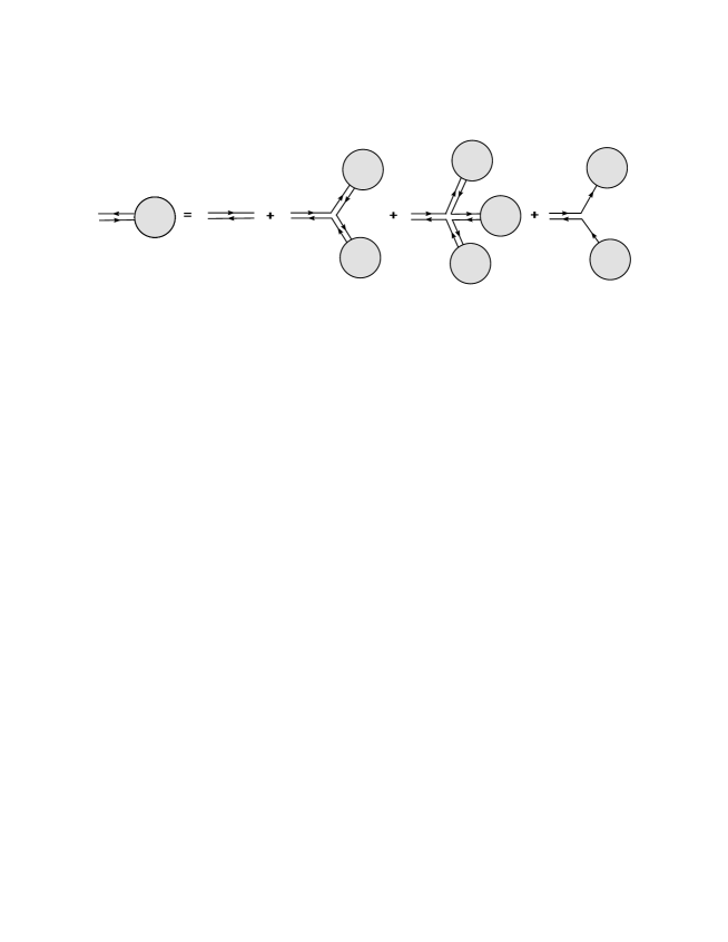
Figure 4: Recursive equation for an off mass shell gluon of momentum P.

The Dyson-Schwinger recursion equation for a gluon can be written as follows:

$$[A^{\mu}(P);(A,B)]=\sum_{i=1}^{n}[~{}\delta_{P=p_{i}}~{}A^{\mu}(p_{i});(A,B)_{i}]$$ (18)

$$+\sum_{P=p_{1}+p_{2}}[~{}(ig)~{}\Pi^{\mu}_{\rho}~{}V^{\rho\nu\lambda}(P,p_{1},p_{2})A_{\nu}(p_{1})A_{\lambda}(p_{2})\sigma(p_{1},p_{2});(A,B)=(C,D)_{1}\otimes(E,F)_{2}]$$

$$-\sum_{P=p_{1}+p_{2}+p_{3}}[~{}(g^{2})~{}\Pi^{\mu}_{\sigma}~{}G^{\sigma\nu\lambda\rho}(P,p_{1},p_{2},p_{3})A_{\nu}(p_{1})A_{\lambda}(p_{2})A_{\rho}(p_{3})\sigma(p_{1},p_{2}+p_{3});$$

$$(A,B)=(C,D)_{1}\otimes(E,F)_{2}\otimes(G,H)_{3}]$$

$$+\sum_{P=p_{1}+p_{2}}[~{}(ig)~{}\Pi^{\mu}_{\nu}~{}\bar{\psi}(p_{1})\gamma^{\nu}\psi(p_{2})\sigma(p_{1},p_{2});(A,B)=(0,D)_{1}\otimes(C,0)_{2}]$$

where $A,B,C,D,E,F,G,H=1,2,3$. The rules for merging colour and anticolour of the particles will be explained in the next section. The $V^{\mu\nu\lambda}(P,p_{1},p_{2})$ and $G^{\mu\nu\lambda\rho}(P,p_{1},p_{2},p_{3})$ functions are the three- and four- gluon vertices presented in the previous sections and the symbol $\sigma(p_{1},p_{2})$ is the sign function which takes into account the Fermi sign when two identical fermions are interchanged. The exact form of this function can be found in Ref.[30, 32]. The sums are over all combinations of $p_{1},p_{2}$ or $p_{1},p_{2},p_{3}$ that sum up to $P$. The propagator of the gluon is given by:

$$\Pi_{\mu\nu}=\frac{-ig_{\mu\nu}}{P^{2}}.$$ (19)

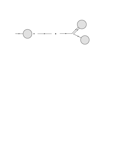
Figure 5: Recursive equation for an off mass shell quark of momentum P.

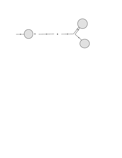
Figure 6: Recursive equation for an off mass shell antiquark of momentum P.

For a quark of momentum $P$ we have, Fig.5:

$$[\psi(P);(A,0)]=\sum_{i=1}^{n}[~{}\delta_{P=p_{i}}~{}\psi(p_{i});(A,0)_{i}]$$ (20)

$$+\sum_{P=p_{1}+p_{2}}[~{}(ig)~{}{\cal P}~{}A^{\mu}(p_{1})\gamma_{\mu}\psi(p_{2})\sigma(p_{1},p_{2});(A,0)=(B,C)_{1}\otimes(D,0)_{2}]$$

where ${\cal P}$ is the propagator

$${\cal P}=\frac{iP\!\!\!/}{P^{2}}.$$ (21)

Finally for an antiquark, Fig.6:

$$[\bar{\psi}(P);(0,A)]=\sum_{i=1}^{n}[~{}\delta_{P=p_{i}}~{}\bar{\psi}(p_{i});(0,A)_{i}]$$ (22)

$$+\sum_{P=p_{1}+p_{2}}[~{}(ig)~{}\bar{\psi}(p_{2})A^{\mu}(p_{1})\gamma_{\mu}~{}\bar{\cal P}\sigma(p_{1},p_{2});(0,A)=(B,C)_{1}\otimes(0,D)_{2}]$$

where

$$\bar{\cal P}=\frac{-iP\!\!\!/}{P^{2}}.$$ (23)

In the same spirit, the recursion equations for all leptons and gauge bosons can be written down. With this algorithm we can thus compute the scattering amplitude for any initial and final states taking into account particle masses as well. In particular any colour structure can be assigned to the external legs. Finally this approach has an exponential growth of computational time with the number of external particles instead of the factorial growth when Feynman graphs are considered. It can be farther optimised in order to reduce computational complexity by replacing each four gluon vertex by a three particle vertex by introducing the auxiliary field represented by the antisymmetric tensor $H^{a}_{\mu\nu}$. This new field has a quadratic term without derivatives and, therefore, has no independent dynamics. The part of the QCD Lagrangian that describes the four gluon vertex

$${\cal L}=-\frac{1}{4}F_{\mu\nu}^{a}F^{\mu\nu a},~{}~{}~{}~{}~{}~{}~{}~{}~{}~{}~{}F^{a}_{\mu\nu}=\partial_{\mu}A_{\nu}^{a}-\partial_{\nu}A_{\mu}^{a}+gf^{abc}A_{\mu}^{b}A_{\nu}^{c}$$ (24)

can be rewritten in terms of the auxiliary field as follows:

$${\cal L}=-\frac{1}{2}H_{\mu\nu}^{a}H^{\mu\nu a}+\frac{1}{4}H_{\mu\nu}^{a}F^{\mu\nu a}.$$ (25)

A single interaction term of the form $H^{\mu\nu a}A^{b}_{\mu}A^{c}_{\nu}$ is left instead of interaction terms represented by Eq.(24). The recursion for the gluons changes slightly, in fact only for the four-gluon vertex part. However, we have an additional equation for the auxiliary field:

$$[A^{\mu}(P);(A,B)]=\sum_{i=1}^{n}[~{}\delta_{P=p_{i}}~{}A^{\mu}(p_{i});(A,B)_{i}]$$ (26)

$$+\sum_{P=p_{1}+p_{2}}[~{}(ig)~{}\Pi^{\mu}_{\rho}~{}V^{\rho\nu\lambda}(P,p_{1},p_{2})A_{\nu}(p_{1})A_{\lambda}(p_{2})\sigma(p_{1},p_{2});(A,B)=(C,D)_{1}\otimes(E,F)_{2}]$$

$$+\sum_{P=p_{1}+p_{2}}[~{}(ig)~{}\Pi^{\mu}_{\sigma}~{}(g^{\sigma\lambda}g^{\nu\rho}-g^{\nu\lambda}g^{\sigma\rho})~{}A_{\nu}(p_{1})H_{\lambda\rho}(p_{2})\sigma(p_{1},p_{2});(A,B)=(C,D)_{1}\otimes(E,F)_{2}]$$

$$+\sum_{P=p_{1}+p_{2}}[~{}(ig)~{}\Pi^{\mu}_{\nu}~{}\bar{\psi}(p_{1})\gamma^{\nu}\psi(p_{2})\sigma(p_{1},p_{2});(A,B)=(0,D)_{1}\otimes(C,0)_{2}]$$

and

$$[H^{\mu\nu}(P);(A,B)]=\sum_{P=p_{1}+p_{2}}[~{}(ig)~{}(g^{\mu\lambda}g^{\nu\rho}-g^{\nu\lambda}g^{\mu\rho})~{}A_{\lambda}(p_{1})A_{\rho}(p_{2})\sigma(p_{1},p_{2});$$ (27)

$$(A,B)=(C,D)_{1}\otimes(E,F)_{2}].$$

A few comments are now in order. First, all calculations were performed in the light cone representation and all momenta were taken to be incoming. Second, this new $H_{\mu\nu}$ field has six components. Additionally, as we can see in Eq.(26) and Eq.(27) the colour structure of this new vertices, remains the same as in case of the three gluon vertex. The number of the types of the sub-amplitudes one has to calculate is in general doubled, however their structure is much simpler, which saves computational time while the iteration steps are performed.

After $n-1$ steps, where $n$ is the number of particles under consideration, one can get the total amplitude. The scattering amplitude can be calculated by any of the following relations, depending on the process under consideration,

$${\cal A}(\{p_{i}\}_{1}^{n},\{\varepsilon_{i}\}_{1}^{n})=\left\{\begin{array}[]{ll}\hat{A}^{\mu}(P_{i})A_{\mu}(p_{i})&\mbox{where $i$ corresponds to gluon}\\ \hat{\bar{\psi}}(P_{i}){\psi}(p_{i})&\mbox{where $i$ corresponds to quark line}\\ \bar{\psi}(p_{i})\hat{\psi}(P_{i})&\mbox{where $i$ corresponds to antiquark line}\\ \end{array}\right.$$ (28)

where

$$P_{i}=\sum_{j\not=i}p_{j},$$

so that $P_{i}+p_{i}=0$. The functions with hat are given by the previous expressions except for the propagator term which is removed by the amputation procedure. This is because the outgoing momentum $P_{i}$ must be on shell. The initial conditions are given by

$$A^{\mu}(p_{i}) = \epsilon^{\mu}_{\lambda}(p_{i}),\lambda=\pm 1,0$$

$$\psi(p_{i}) = \left\{\begin{array}[]{ll}u_{\lambda}(p_{i})&\mbox{if $p_{i}^{0}\geq 0$}\\ v_{\lambda}(-p_{i})&\mbox{if $p_{i}^{0}\leq 0$}\\ \end{array}\right.$$ (31)

$$\bar{\psi}(p_{i}) = \left\{\begin{array}[]{ll}\bar{u}_{\lambda}(p_{i})&\mbox{if $p_{i}^{0}\geq 0$}\\ \bar{v}_{\lambda}(-p_{i})&\mbox{if $p_{i}^{0}\leq 0$}\\ \end{array}\right.$$ (34)

where the explicit form of $\epsilon^{\mu}_{\lambda},u_{\lambda},v_{\lambda},\bar{u}_{\lambda},\bar{v}_{\lambda}$ is given in the Ref.[30].

5 Organisation of the calculation

The recursive algorithm presented in the previous section has the advantage that any colour representation can be used in order to assign colour degrees of freedom to the external legs in the process under consideration. It can be used either for colour ordered amplitudes or for the full amplitudes as well. The latter case is in fact the topic of this section. Moreover, an alternative method for taking into account the colour structure of scattering partons, based on regular colour configuration assignments as compared to colour flow ones, will be introduced. First, however, the organisation of the calculation will be explained briefly in order to better describe the general structure. Contrary to the original HELAC [30, 31] approach, in this new version the computational part consists of one phase only. This is not optimal for electroweak processes with moderate number of external particles, but it becomes quite efficient for processes with many particles, especially when only a few species of particles are involved (scalar amplitudes, gluon amplitudes in QCD, etc). The vertices described by the Standard Model Lagrangian are implemented in fusion rules that dictate the way the subamplitudes, at each level of the recursion relation, will be merged, in order to produce a higher level subamplitude. In case when a quark is combined with an antiquark, for example, there are three possible subamplitudes which describe three different intermediate states incorporated inside the fusion rules, namely $\gamma$, $Z$ and $g$.

Let us now present the colour merging rules which are evaluated iteratively at the subamplitude level. During each iteration when two particles are combined their corresponding colour assignments are combined. We have three possibilities to obtain a gluon $(A,B)$ described by the recursive relation Eq.(26). First, it can be obtained when a quark with colour assignment $(C,0)$ is merged with an antiquark of anticolour $(0,D)$. Second, when two gluons $(C,D)$ and $(E,F)$ are combined, where $A,B,C,D,E,F=1,2,3$, and finally when a gluon and an auxiliary field $H$ are combined. In the last case, the colour structure of the vertex is identical to the three-gluon vertex. So we end up with the following rules:

$$(A,B)\leftarrow(C,0~{})\otimes(~{}0,D),$$ (35)

$$(A,B)\leftarrow(C,D)\otimes(E,F).$$ (36)

In the first case the merging occurs according to the rule presented in Eq.(8). and the following gluon can be produced:

$$(A,B)=(C,0)\otimes(0,D)=(C,D),~{}~{}~{}~{}~{}~{}{\textnormal{if}}~{}C\neq D.$$ (37)

However, the situation is more complex when a quark and an antiquark have the same colour and anticolour:

$$(A,B)=(C,0)\otimes(0,D)=(1,1)_{w_{1}}\oplus(2,2)_{w_{2}}\oplus(3,3)_{w_{3}},~{}~{}~{}~{}~{}~{}{\textnormal{if}}~{}C=D.$$ (38)

with $\sum w_{i}=0$. We thus have three possibilities with different weights, which for instance are $w_{1}=w_{2}=-1/3$, $w_{3}=+2/3$ in case $C=D=3$.

In the second case, when gluons are combined according to Eq.(6) we have the following options:

$$(A,B)=(C,D)\otimes(E,F)=(E,D),~{}~{}~{}~{}~{}~{}{\textnormal{if}}~{}C=F~{}~{}~{}~{}~{}{\textnormal{and}}~{}E\neq D$$ (39)

$$(A,B)=(C,D)\otimes(E,F)=(C,F),~{}~{}~{}~{}~{}~{}{\textnormal{if}}~{}D=E~{}~{}~{}~{}~{}{\textnormal{and}}~{}C\neq F.$$ (40)

Moreover, we have an additional possibility when colours and anticolours of gluons are the same. One gets, in this case, a gluon in two colour states with different weight:

$$(A,B)=(C,D)\otimes(E,F)=(C,C)_{+1}\oplus(D,D)_{-1},~{}~{}~{}{\textnormal{if}}~{}~{}~{}C=F~{}~{}~{}E=D~{}~{}~{}{\textnormal{and}}~{}~{}~{}C\neq D.$$ (41)

Finally for $C=D=E=F$ the result vanishes identically.

To obtain the quark, $(A,0)$, described by the recursive relation Eq.(20) we have to combine a gluon with another quark one more time according to the rule presented in Eq.(8):

$$(A,0)=(B,C)\otimes(D,0).$$ (42)

We have two possibilities for colour assignment:

$$(A,0)=(B,C)\otimes(D,0)=(B,0),~{}~{}~{}~{}~{}~{}{\textnormal{if}}~{}C=D,$$ (43)

$$(A,0)=(B,C)\otimes(D,0)=(D,0),~{}~{}~{}~{}~{}~{}{\textnormal{if}}~{}B=C.$$ (44)

For the antiquark the situation is the same, so we will not elaborate it here.

For the $q\bar{q}$ interactions with $\gamma,Z^{0},W^{\pm}$ or Higgs boson the situation is very simple and we have only one possibility:

$$(A,0)\otimes(0,B)=(0,0)~{}~{}~{}~{}~{}~{}~{}~{}~{}~{}~{}~{}~{}~{}~{}\textnormal{if}~{}A=B.$$ (45)

The sum over colour can be performed in this way by considering all possible colour-anticolour configurations according to the above rules. However, the procedure can be facilitated by Monte Carlo methods where a particular colour-anticolour configuration is randomly selected. As we will see an important gain in computational efficiency is achieved within this framework.

The necessary condition which must be fulfilled, while the particular colour assignment for the external coloured particles is chosen, is that the number of colour and anticolour of each type, is the same. Otherwise the particles can not be connected by colour flow lines and the amplitude is identically zero. In the Monte Carlo over colours method one has to multiply the squared matrix element by a coefficient that counts the number of non zero colour configurations.

The number of non zero colour configurations, according to the above mentioned necessary condition is given by

$$N_{\textnormal{\tiny CC}}=\sum_{A=0}^{n_{q}}~{}\sum_{B=0}^{n_{q}-A}~{}\sum_{C=0}^{n_{q}-A-B}\bigg{(}\frac{n_{q}!}{A!B!C!}\bigg{)}^{2}~{}\delta(n_{q}=A+B+C)$$ (46)

where $n_{q}$ is the total number of colours and $A,B,C$ are the numbers of the colour type $1$, $2$ and $3$ respectively. As we already stated, the condition given by Eq.(46) is necessary but not sufficient. Among this set there are still configurations which do not give contributions to the total amplitude.

Table 2: The number of colour configurations for the processes with gluons only. $N_{\textnormal{{\tiny CC}}}^{\textnormal{{\tiny ALL}}}$ corresponds to all possible colour configurations, while $N_{\textnormal{{\tiny CC}}}$ corresponds to the number of colour configurations calculated using formula Eq.(46). In the third column the ratio $\textnormal{N}_{\textnormal{\tiny CC}}/\textnormal{N}^{\textnormal{\tiny ALL}}_{\textnormal{\tiny CC}}$ is presented. In the last column the number of non vanishing colour configurations evaluated by MC $\textnormal{N}_{\textnormal{\tiny CC}}^{\textnormal{\tiny F}}$ (in percentage) inside the $\textnormal{N}_{\textnormal{\tiny CC}}$ is shown.

Process	$\textnormal{N}^{\textnormal{\tiny ALL}}_{\textnormal{\tiny CC}}$	$\textnormal{N}_{\textnormal{\tiny CC}}$	$\textnormal{N}_{\textnormal{\tiny CC}}/\textnormal{N}^{\textnormal{\tiny ALL}}_{\textnormal{\tiny CC}}$	$\textnormal{N}_{\textnormal{\tiny CC}}^{\textnormal{\tiny F}}$ ($\%$)
$gg\rightarrow 2g$	6561	639	0.0974	59.1
$gg\rightarrow 3g$	59049	4653	0.0788	68.4
$gg\rightarrow 4g$	531441	35169	0.0662	77.4
$gg\rightarrow 5g$	4782969	272835	0.0570	85.0
$gg\rightarrow 6g$	43046721	2157759	0.0501	90.4
$gg\rightarrow 7g$	387420489	17319837	0.0447	94.0
$gg\rightarrow 8g$	3486784401	140668065	0.0403	96.4

Table 3: The number of colour configurations for the processes with gluons and one or two $q\bar{q}$ pairs. $N_{\textnormal{{\tiny CC}}}^{\textnormal{{\tiny ALL}}}$ corresponds to all possible colour configurations, while $N_{\textnormal{{\tiny CC}}}$ corresponds to the number of colour configurations calculated using formula Eq.(46). In the third column the ratio $N_{\textnormal{{\tiny CC}}}/N_{\textnormal{{\tiny CC}}}^{\textnormal{{\tiny ALL}}}$ is presented. In the last column the number of non vanishing colour configurations evaluated by MC $\textnormal{N}_{\textnormal{\tiny CC}}^{\textnormal{\tiny F}}$ (in percentage) inside the $\textnormal{N}_{\textnormal{\tiny CC}}$ is shown.

Process	$\textnormal{N}^{\textnormal{\tiny ALL}}_{\textnormal{\tiny CC}}$	$\textnormal{N}_{\textnormal{\tiny CC}}$	$\textnormal{N}_{\textnormal{\tiny CC}}/\textnormal{N}^{\textnormal{\tiny ALL}}_{\textnormal{\tiny CC}}$	$\textnormal{N}_{\textnormal{\tiny CC}}^{\textnormal{\tiny F}}$ ($\%$)
$gg\rightarrow u\bar{u}$	729	93	0.1276	93.5
$gg\rightarrow gu\bar{u}$	6561	639	0.0974	91.6
$gg\rightarrow 2gu\bar{u}$	59049	4653	0.0788	92.6
$gg\rightarrow 3gu\bar{u}$	531441	35169	0.0662	94.6
$gg\rightarrow 4gu\bar{u}$	4782969	272835	0.0570	96.4
$gg\rightarrow 5gu\bar{u}$	43046721	2157759	0.0501	97.8
$gg\rightarrow 6gu\bar{u}$	387420489	17319837	0.0447	98.6
$gg\rightarrow c\bar{c}c\bar{c}$	6561	639	0.0974	99.1
$gg\rightarrow gc\bar{c}c\bar{c}$	59049	4653	0.0788	98.8
$gg\rightarrow 2gc\bar{c}c\bar{c}$	531441	35169	0.0662	99.0
$gg\rightarrow 3gc\bar{c}c\bar{c}$	4782969	272835	0.0570	99.3
$gg\rightarrow 4gc\bar{c}c\bar{c}$	43046721	2157759	0.0501	99.6

In Tab. 2. and Tab. 3. different numbers of colour configurations in the process under consideration are presented. In the first column the total number of all colour configurations is listed, where $\textnormal{N}^{\textnormal{\tiny ALL}}_{\textnormal{\tiny CC}}=3^{n_{q}+n_{\bar{q}}}$ and $n_{q}$, $n_{\bar{q}}$ are the number of quarks and antiquarks respectively and gluons are treated as $q\bar{q}$ pairs. The second column represents results for the number of non vanishing colour configurations $\textnormal{N}_{\textnormal{\tiny CC}}$ calculated using Eq.(46). In the next column the ratio $N_{\textnormal{{\tiny CC}}}/N_{\textnormal{{\tiny CC}}}^{\textnormal{{\tiny ALL}}}$ is presented. The number of colour configurations (in percentage) inside the $\textnormal{N}_{\textnormal{\tiny CC}}$ set which finally gives rise to non zero amplitudes is shown in the last column. Those numbers $\textnormal{N}_{\textnormal{\tiny CC}}^{\textnormal{\tiny F}}$ are evaluated by Monte Carlo. Note that while the number of external particles is increased the corresponding number of vanishing colour configurations in the third column is decreased, as we can see in Tab. 2.

As far as the summation over the helicity configurations is concerned there are two possibilities, either the explicit summation over all helicity configurations or a Monte Carlo approach. In the latter case, for example for gluon, it is achieved by introducing the polarisation vector

$$\varepsilon^{\mu}_{\phi}(p)=e^{i\phi}\varepsilon^{\mu}_{+}(p)+e^{-i\phi}\varepsilon^{\mu}_{-}(p),$$ (47)

where $\phi\in(0,2\pi)$. By integrating over $\phi$ we can obtain the sum over helicities

$$\frac{1}{2\pi}\int_{0}^{2\pi}d\phi~{}\varepsilon^{\mu}_{\phi}(p)(\varepsilon^{\nu}_{\phi}(p))^{*}=\sum_{\lambda=\pm}\varepsilon_{\lambda}^{\mu}(p)(\varepsilon_{\lambda}^{\nu}(p))^{*}.$$

To determine the cost of computation of the $n-$point amplitude using the algorithm based on Dyson-Schwinger equations, one has to count the number of operations [35]. There are $\left(\begin{array}[]{l}n\\ k\end{array}\right)$ momenta at each level. The total amount of sub-amplitudes corresponding to those momenta is simply given by:

$$\sum_{k=1}^{n-1}\left(\begin{array}[]{l}n\\ k\end{array}\right)=2^{n}-2$$ (48)

where $n$ is the number of particles involved in the calculation. Moreover one has to count how many ways exist to split a number of level $k$ to two numbers of levels $k_{1}$ and $k_{2}$. The last step is to sum over all levels. The total number of operations that should be performed in the case when only three-point vertices exist is then

$$\sum_{k=1}^{n-1}\left(\begin{array}[]{l}n\\ k\end{array}\right)\sum_{l=1}^{k-1}\left(\begin{array}[]{l}k\\ l\end{array}\right)=\sum_{k=1}^{n-1}\left(\begin{array}[]{l}n\\ k\end{array}\right)\{2^{k}-2\}=3^{n}-3\cdot 2^{n}+3.$$ (49)

In the limit $n\rightarrow\infty$ the number of operations grows like $3^{n}$ instead of the $n!$ growth in the Feynman graph approach. When the Monte Carlo over colour structures is performed and only one particular colour configuration is randomly chosen the computational cost of this algorithm is given exactly by this expression. Otherwise, this formula must be multiplied by the number of non zero colour configurations for the process under consideration.

6 Numerical Results

Table 4: Results for the total cross section for processes with gluons and quarks with up to two $q\bar{q}$ pairs. $\sigma_{\textnormal{{\tiny EXACT}}}$ corresponds to summation over all possible colour configurations, while $\sigma_{\textnormal{{\tiny MC}}}$ corresponds to Monte Carlo summation.

Process	$\sigma_{\textnormal{\tiny EXACT}}$ $\pm$ $\varepsilon$ (nb)	$\varepsilon~{}(\%)$	$\sigma_{\textnormal{\tiny MC}}$ $\pm$ $\varepsilon$ (nb)	$\varepsilon~{}(\%)$
$gg\rightarrow 2g$	(0.46572 $\pm$ 0.00258)$\times 10^{4}$	0.5	(0.46849 $\pm$ 0.00308)$\times 10^{4}$	0.6
$gg\rightarrow 3g$	(0.15040 $\pm$ 0.00159)$\times 10^{3}$	1.0	(0.15127 $\pm$ 0.00110)$\times 10^{3}$	0.7
$gg\rightarrow 4g$	(0.11873 $\pm$ 0.00224)$\times 10^{2}$	1.9	(0.12116 $\pm$ 0.00134)$\times 10^{2}$	1.1
$gg\rightarrow 5g$	(0.10082 $\pm$ 0.00198)$\times 10^{1}$	1.9	(0.09719 $\pm$ 0.00142)$\times 10^{1}$	1.5
$gg\rightarrow 6g$	(0.74717 $\pm$ 0.01490)$\times 10^{-1}$	2.0	(0.76652 $\pm$ 0.01862)$\times 10^{-1}$	2.4
$gg\rightarrow u\bar{u}$	(0.36435 $\pm$ 0.00199)$\times 10^{2}$	0.5	(0.36619 $\pm$ 0.00132)$\times 10^{2}$	0.4
$gg\rightarrow gu\bar{u}$	(0.35768 $\pm$ 0.00459)$\times 10^{1}$	1.3	(0.35466 $\pm$ 0.00291)$\times 10^{1}$	0.8
$gg\rightarrow 2gu\bar{u}$	(0.49721 $\pm$ 0.00758)$\times 10^{0}$	1.5	(0.50053 $\pm$ 0.00725)$\times 10^{0}$	1.4
$gg\rightarrow 3gu\bar{u}$	(0.50598 $\pm$ 0.01441)$\times 10^{-1}$	2.8	(0.52908 $\pm$ 0.01264)$\times 10^{-1}$	2.4
$gg\rightarrow 4gu\bar{u}$	(0.51549 $\pm$ 0.02017)$\times 10^{-2}$	3.9	(0.51581 $\pm$ 0.01245)$\times 10^{-2}$	2.4
$gg\rightarrow c\bar{c}c\bar{c}$	(0.25190 $\pm$ 0.00528)$\times 10^{-2}$	2.1	(0.24903 $\pm$ 0.00373)$\times 10^{-2}$	1.5
$gg\rightarrow gc\bar{c}c\bar{c}$	(0.60196 $\pm$ 0.01908)$\times 10^{-3}$	3.2	(0.58817 $\pm$ 0.00926)$\times 10^{-3}$	1.6
$gg\rightarrow 2gc\bar{c}c\bar{c}$	(0.95682 $\pm$ 0.03441)$\times 10^{-4}$	3.6	(0.92212 $\pm$ 0.02485)$\times 10^{-4}$	2.7

Table 5: Comparison of the computational time for the squared matrix element calculation for processes with gluons and/or quarks with up to two $q\bar{q}$ pairs, $\textnormal{t}_{\textnormal{\tiny EXACT}}$ denotes the time for the processes calculated with summation over all possible colour flows (for colour ordered amplitudes), while $\textnormal{t}_{\textnormal{\tiny MC}}$ is obtained with Monte Carlo summation over colours (for full amplitudes). In the last column their ratio is presented. Time values are given in some arbitrary units.

Process	$\textnormal{t}^{\textnormal{\tiny CF}}_{\textnormal{\tiny EXACT}}$	$\textnormal{t}_{\textnormal{\tiny MC}}$	$\textnormal{t}_{\textnormal{\tiny EXACT}}/\textnormal{t}_{\textnormal{\tiny MC}}$
$gg\rightarrow 2g$	0.315$\times 10^{0}$	0.554$\times 10^{0}$	0.57
$gg\rightarrow 3g$	0.329$\times 10^{1}$	0.143$\times 10^{1}$	2.30
$gg\rightarrow 4g$	0.383$\times 10^{2}$	0.372$\times 10^{1}$	10.29
$gg\rightarrow 5g$	0.517$\times 10^{3}$	0.105$\times 10^{2}$	49.24
$gg\rightarrow 6g$	0.987$\times 10^{4}$	0.362$\times 10^{2}$	272.65
$gg\rightarrow u\bar{u}$	0.260$\times 10^{0}$	0.466$\times 10^{0}$	0.56
$gg\rightarrow gu\bar{u}$	0.196$\times 10^{1}$	0.123$\times 10^{0}$	1.59
$gg\rightarrow 2gu\bar{u}$	0.166$\times 10^{2}$	0.348$\times 10^{1}$	4.77
$gg\rightarrow 3gu\bar{u}$	0.171$\times 10^{3}$	0.129$\times 10^{2}$	13.25
$gg\rightarrow 4gu\bar{u}$	0.197$\times 10^{4}$	0.307$\times 10^{2}$	64.17
$gg\rightarrow c\bar{c}c\bar{c}$	0.697$\times 10^{1}$	0.605$\times 10^{1}$	1.15
$gg\rightarrow gc\bar{c}c\bar{c}$	0.568$\times 10^{2}$	0.217$\times 10^{2}$	2.62
$gg\rightarrow 2gc\bar{c}c\bar{c}$	0.619$\times 10^{3}$	0.401$\times 10^{2}$	15.44

Table 6: Results for the total cross section for processes with gluons, $Z$, $W^{\pm}$ and quarks with up to $q\bar{q}$ pairs for the higher number of external partons. $\sigma_{\textnormal{{\tiny MC}}}$ corresponds to Monte Carlo summation over colours.

Process	$\sigma_{\textnormal{\tiny MC}}$ $\pm$ $\varepsilon$ (nb)	$\varepsilon~{}(\%)$
$gg\rightarrow 7g$	(0.53185 $\pm$ 0.01149)$\times 10^{-2}$	2.1
$gg\rightarrow 8g$	(0.33330 $\pm$ 0.00804)$\times 10^{-3}$	2.4
$gg\rightarrow 9g$	(0.13875 $\pm$ 0.00430)$\times 10^{-4}$	3.1
$gg\rightarrow 5gu\bar{u}$	(0.38044 $\pm$ 0.01096)$\times 10^{-3}$	2.8
$gg\rightarrow 3gc\bar{c}c\bar{c}$	(0.95109 $\pm$ 0.02456)$\times 10^{-5}$	2.6
$gg\rightarrow 4gc\bar{c}c\bar{c}$	(0.81400 $\pm$ 0.02583)$\times 10^{-6}$	3.2
$gg\rightarrow Zu\bar{u}gg$	(0.18948 $\pm$ 0.00344)$\times 10^{-3}$	1.8
$gg\rightarrow W^{+}\bar{u}dgg$	(0.62704 $\pm$ 0.01458)$\times 10^{-3}$	2.3
$gg\rightarrow ZZu\bar{u}gg$	(0.16217 $\pm$ 0.00420)$\times 10^{-6}$	2.6
$gg\rightarrow W^{+}W^{-}u\bar{u}gg$	(0.27526 $\pm$ 0.00752)$\times 10^{-5}$	2.7
$d\bar{d}\rightarrow Zu\bar{u}gg$	(0.38811 $\pm$ 0.00569)$\times 10^{-5}$	1.5
$d\bar{d}\rightarrow W^{+}\bar{c}sgg$	(0.18765 $\pm$ 0.00453)$\times 10^{-5}$	2.4
$d\bar{d}\rightarrow ZZgggg$	(0.99763 $\pm$ 0.02976)$\times 10^{-7}$	2.9
$d\bar{d}\rightarrow W^{+}W^{-}gggg$	(0.52355 $\pm$ 0.01509)$\times 10^{-6}$	2.9

In this section numerical results for multi-parton production at the LHC are presented. As we will show the Monte Carlo summation over colours, speeds up the calculation substantially, compared to the one based on explicit summation, especially for processes with a large number of colors, i.e. $gg\to ng$ with $n>6$.

The centre of mass energy was chosen to be $\sqrt{s}=14$ TeV. In order to remain far from collinear and soft singularities and to simulate as much as possible the experimentally relevant phase-space regions, we have chosen the following cuts:

$$p_{T_{i}}>60~{}\textnormal{GeV},~{}~{}~{}~{}|y_{i}|<2.5,~{}~{}~{}~{}\Delta R_{ij}>1.0$$ (50)

for each pair of outgoing partons $i$ and $j$. Here $p_{T_{i}}$ and $y_{i}$ are the transverse momentum and rapidity of a parton respectively defined as:

$$p_{T_{i}}=\sqrt{p_{x_{i}}^{2}+p_{y_{i}}^{2}},~{}~{}~{}~{}~{}y_{i}=\frac{1}{2}\ln\left(\frac{E_{i}+p_{z_{i}}}{E_{i}-p_{z_{i}}}\right).$$ (51)

In practice for massless quarks the rapidity is often replaced by the pseudorapidity variable $\eta=-\ln\tan(\theta/2)$, where $\theta$ is the angle from the beam direction measured directly in the detector. The last variable is $\Delta R_{ij}$ which is the radius of the cone of the parton defined as

$$\Delta R_{ij}=\sqrt{(\Phi_{i}-\Phi_{j})^{2}+(\eta_{i}-\eta_{j})^{2}}$$ (52)

with azimuthal angle $\Delta\Phi_{ij}=\Phi_{i}-\Phi_{j}\in(0,\pi)$

$$\Delta\Phi_{ij}=\arccos\biggl{(}\frac{p_{x_{i}}p_{x_{j}}+p_{y_{i}}p_{y_{j}}}{p_{T_{i}}p_{T_{j}}}\biggr{)}.$$ (53)

Quarks are treated as massless. All results are obtained with a fixed strong coupling constant ($\alpha_{s}$=0.13). For the parton structure functions, we used CTEQ6L1 PDF’s parametrisation [36, 37]. For the phase space generation we used the algorithm described in the Appendix, whereas in several cases results were cross checked with

• PHEGAS [38], which automatically constructs mappings of all possible peaking structures of a given scattering process and uses self-adaptive procedures like multi-channel optimisation [39]. PHEGAS exhibits a high efficiency especially in the case of $n(+\gamma)-$fermion production in $e^{+}e^{-}$ collisions as long as the number of external particles is smaller than ${\cal O}(8)$.

• HAAG[40], which efficiently maps the so called “antenna momentum structures” typically occurring in the QCD amplitudes. HAAG becomes less efficient for processes with higher number of particles, more than ${\cal O}(8)$, as is the case for any multi-channel generator, where the computational complexity problem arises when the number of channels increases.

• RAMBO [41], a flat phase-space generator RAMBO generates the momenta distributed uniformly in phase space so that a large number of events is needed to integrate the integrands to acceptable precision, which results to a rather low computational efficiency.

Total rates and various kinematical distributions are examined. The algorithm described in the previous sections as well as in Ref.[42, 43] has been used to compute total cross sections for many parton production processes. We give the result with summation over all possible colour configurations, called ’exact’, $\sigma_{\textnormal{{\tiny EXACT}}}$, as well as the result obtained with Monte Carlo summation over colours $\sigma_{\textnormal{{\tiny MC}}}$.

In case of the explicit summation both colour flow and colour configuration decomposition have been used to cross check results. As far as helicity summation is concerned, a Monte Carlo over helicities is applied.

The results presented for the total cross sections, have been obtained for $10^{6}$ Monte Carlo points passing the selection cuts given by Eg.(50). In the Tab. 4. the results for the total cross section for processes with gluons and/or quarks with up to two $q\bar{q}$ pairs are presented. All cross sections are in agreement within the error. For the same number of accepted events the results with the Monte Carlo summation over colours can be obtained much faster and the error is at the same level compared to the ’exact’ results for the same processes.

In the Tab. 5. a comparison of the computational time for squared matrix element calculations for processes with gluons and/or quarks with up to two $q\bar{q}$ pairs is presented. In each case $\textnormal{t}_{\textnormal{\tiny EXACT}}$ means time obtained for the processes calculated with the summation over all possible colour flows (for colour ordered amplitudes), while $\textnormal{t}_{\textnormal{\tiny MC}}$ is obtained with Monte Carlo summation over colours (for full amplitudes).

In the next Tab. 6. the results for the total cross section for processes with gluon, $Z$, $W^{\pm}$ and quarks with up to $q\bar{q}$ pairs for a larger number of external partons are also presented.

Figure 7: Distribution in $z=|{\cal M}_{\textnormal{\tiny one}}|^{2}/\sum_{i}^{all}|{\cal M}_{i}|^{2}$, where $|{\cal M}_{\textnormal{\tiny one}}|^{2}$ is the square matrix element for one particular colour configuration normalised to the sum of all possible. The left-hand side plot corresponds to the $gg\rightarrow 2g$ process, the right-hand side one to the $gg\rightarrow 3g$. Solid line crosses denote summation over all colour configurations whereas dashed, the Monte Carlo summation.

Figure 8: Invariant mass distribution of 2 gluons in the multigluon $2g\rightarrow ng$ process.

Figure 9: Transverse momentum distribution of a gluon in the multigluon $2g\rightarrow ng$ process.

Figure 10: Transverse momentum distribution of the hardest gluon in the multigluon $2g\rightarrow ng$ process.

Figure 11: Transverse momentum distribution of the softest gluon in the multigluon $2g\rightarrow ng$ process.

In order to demonstrate that the Monte Carlo summation over colours does give the same information on the colour connection structure of the process, we examine in Fig. 7 the distribution of the following variable,

$$z=\frac{|{\cal M}_{\textnormal{\tiny one}}|^{2}}{\sum_{i=1}^{all}|{\cal M}_{i}|^{2}}$$ (54)

where $|{\cal M}_{\textnormal{\tiny one}}|^{2}$ is the square matrix element for one particular colour connection or colour flow configuration, normalised to the sum of all possible ones. In case of $g(1)g(2)\rightarrow g(3)g(4)$ process, the following colour flow $(1\rightarrow 3\rightarrow 4\rightarrow 2\rightarrow 1)$ has been plotted. This chain of numbers shows how gluons are colour connected with each other. For the $g(1)g(2)\rightarrow g(3)g(4)g(5)$ process in the Fig. 7, the colour flow $(1\rightarrow 5\rightarrow 3\rightarrow 2\rightarrow 4\rightarrow 1)$ is used.

The $z-$variable distributions can be used in order to extract colour connection information needed by a parton shower calculation on the event by event basis. The agreement between the ’exact’ and MC distributions implies that we will get the same information on the colour structure of the amplitude and that the merging of parton level calculation with the parton shower evolution can be safely performed in order to achieve a complete description of the fully hadronised final states observed in real experiments.

Finally, the distribution of the invariant mass of 2-partons, the transverse momentum distribution of one parton as well as of the hardest and the softest parton for $gg\rightarrow ng$, $n=4,\ldots,8$ process is shown in Fig. 8.$-$Fig. 11. Distributions of the Monte Carlo over colours clearly demonstrate that this approach performs very well not only at the level of total rates but also at the level of differential distributions.

Summary and Outlook

In this work an efficient way for the computation of tree level amplitudes for multi-parton processes in the Standard Model was presented. The algorithm is based on the Dyson-Schwinger recursive equations. We discussed how the summation over colour configurations can be turned into a Monte Carlo summation, which proved to be more efficient, especially for a large number of coloured partons. Additionally, a set of typical results for total cross sections and differential distributions has been given. Moreover, a new algorithm for phase-space generation has been presented and used. The complete package can be used to generate, efficiently and reliably, any process with any number of external legs, for $n\leq~{}12$, in the Standard Model.

Our future interest includes a systematic study of fully hadronic final states in $p\bar{p}$ and $pp$ collisions which requires the merging of the parton level calculations with parton shower and hadronization algorithms, e.g interfacing our package with codes like PYTHIA[44] or HERWIG[45]. The development of this kind of multipurpose Monte Carlo generators will certainly be of great interest in the study of TeVatron, LHC and $e^{+}e^{-}$ Linear Collider data.

Appendix

In case of scattering of two hadrons it is useful to describe the final state in terms of transverse momentum $p_{T}$, azimuthal angle $\phi$ and rapidity $y$ variables. These variables transform simply under longitudinal boosts which is useful in case of the parton-parton scattering where the centre of mass system is boosted with respect to that of the two incoming hadrons. In terms of $p_{T}$, $\phi$ and $y$ the four-momentum of a massless particle can be written as

$$p^{\mu}=(E,p^{x},p^{y},p^{z})=(p_{T}\cosh y,p_{T}\cos\phi,p_{T}\sin\phi,p_{T}\sinh y)$$ (55)

It is much more natural to express the phase space volume for a system of $n$ particles

$$V_{n}=\int\delta^{4}(P-\sum_{i=1}^{n}p_{i})\prod_{i=1}^{n}d^{4}p_{i}\delta(p_{i}^{2}-m^{2}_{i})\Theta(p^{0}_{i})$$ (56)

using $p_{T}$, $\phi$ and $y$ variables

$$V_{n}=\int\delta^{4}(P-\sum_{i=1}^{n}p_{i})\prod_{i=1}^{n}p_{T_{i}}dp_{T_{i}}dy_{i}d\phi_{i}.$$ (57)

To derive the above expression, which lead us to the Monte Carlo algorithm, we follow the method presented in Ref. [41]. We start by defining the phase-space-like object

$$V_{0}=\int_{0}^{\infty}\left(\prod_{i=2}^{n}dk_{T_{i}}~{}P(k_{T_{i}})\right)\int_{0}^{2\pi}\left(\prod_{i=2}^{n}d\phi_{i}\right)\int_{-\infty}^{+\infty}\left(\prod_{i=2}^{n}d{\bar{y}}_{i}~{}\Pi(\bar{y}_{i})\right)$$ (58)

describing a system of $n$ four momenta that are not constrained by momentum conservation but occur with some weight functions $P(k_{T_{i}})$, $\Pi({\bar{y}}_{i})$ which keeps the total volume finite. In the next step we have to relate the new variables to the physical ones $p_{T_{i}}$, $y_{i}$ and $\phi_{i}$:

$$V_{0}=\int_{0}^{\infty}\left(\prod_{i=2}^{n}dk_{T_{i}}~{}P(k_{T_{i}})\right)\int_{0}^{2\pi}\left(\prod_{i=2}^{n}d\phi_{i}\right)\int_{-\infty}^{+\infty}\left(\prod_{i=2}^{n}d{\bar{y}}_{i}~{}\Pi(\bar{y}_{i})\right)$$

$$\int_{0}^{\infty}\left(\prod_{i=1}^{n}dp_{T_{i}}~{}\delta(p_{T_{i}}-xk_{T_{i}})\right)\int_{-\infty}^{+\infty}\left(\prod_{i=2}^{n}dy_{i}~{}\delta(\bar{y}_{i}+y_{i-1}-y_{i})\right)$$

$$\!\!\!\!\!\!\int_{0}^{\infty}dk_{T_{1}}\int_{0}^{2\pi}d\phi_{1}~{}\delta(x\sum_{i=2}^{n}k_{T_{i}}\cos{\phi_{i}})~{}\delta(x\sum_{i=2}^{n}k_{T_{i}}\sin{\phi_{i}})~{}{\cal J}_{1}$$ (59)

$$~{}~{}~{}~{}~{}~{}~{}~{}\int_{0}^{\infty}dx\int_{-\infty}^{+\infty}dy_{1}~{}\delta(x\sum_{i=2}^{n}k_{T_{i}}\cosh y_{i}-E)~{}\delta(x\sum_{i=2}^{n}k_{T_{i}}\sinh y_{i}-L)~{}{\cal J}_{2}.$$

with the Jacobians ${\cal J}_{1}$ and ${\cal J}_{2}$:

$${\cal J}_{1}=\left|\frac{\partial(x\sum k_{T_{i}}\cos{\phi_{i}},x\sum k_{T_{i}}\sin{\phi_{i}})}{\partial(k_{T_{1}},\phi_{1})}\right|=x^{2}k_{T_{1}}$$ (60)

$${\cal J}_{2}=\left|\frac{\partial(x\sum k_{T_{i}}\cosh{y_{i}}-E,x\sum k_{T_{i}}\sinh{y_{i}}-L)}{\partial(x,y_{1})}\right|=\frac{E^{2}-L^{2}}{x}.$$ (61)

$E$ and $L$ represents the energy and longitudinal parts of the initial two particles. We proceed with integration where the different arguments of the various $\delta$ functions were manipulated in order to perform the integral

$$\int_{0}^{\infty}\prod_{i=1}^{n}dk_{T_{i}}~{}\delta(p_{T_{i}}-xk_{T_{i}})$$ (62)

$$\int_{-\infty}^{+\infty}\prod_{i=2}^{n}d{\bar{y}}_{i}~{}\delta({\bar{y}}_{i}+y_{i-1}-y_{i}).$$ (63)

We are left with

$$V_{0}=\int\delta^{4}(P-\sum_{i=1}^{n}p_{i})\left(\prod_{i=1}^{n}p_{T_{i}}dp_{T_{i}}dy_{i}d\phi_{i}\right)\left(\prod_{i=2}^{n}P\left(\frac{p_{T_{i}}}{x}\right)\frac{1}{p_{T_{i}}}\Pi(\bar{y}_{i})\right)(E^{2}-L^{2})\frac{2^{n}}{x^{n}}dx.$$ (64)

We are free to choose the distribution functions so that the total volume is kept finite. The criterion used is to minimize the variance, by taking into account the anticipated form of the multi-parton matrix elements, so we introduce

$$P(x)=\frac{1}{a}\exp\left(\frac{-x}{a}\right),~{}~{}~{}~{}~{}~{}~{}\Pi({\bar{y}})=\frac{\tanh(2\eta+\bar{y})+\tanh(2\eta-\bar{y})}{8\eta}$$ (65)

where $a>0$ and perform the integration over $dx$

$$\int_{0}^{\infty}\left(\prod_{i=2}^{n}\frac{1}{a}\exp\left(\frac{-p_{T_{i}}}{xa}\right)\frac{1}{p_{T_{i}}}\right)\frac{1}{x^{n}}dx=\left(\prod_{i=2}^{n}\frac{1}{p_{T_{i}}}\right)\left(\sum_{i=2}^{n}p_{T_{i}}\right)^{-n+1}\Gamma(n-1).$$ (66)

We finally arrive at the formula

$$V_{0}=\int\delta^{4}(P-\sum_{i=1}^{n}p_{i})\left(\prod_{i=1}^{n}p_{T_{i}}dp_{T_{i}}dy_{i}d\phi_{i}\right)~{}\times$$ (67)

$$\left(\prod_{i=2}^{n}\frac{1}{p_{T_{i}}}\right)\left(\sum_{i=2}^{n}p_{T_{i}}\right)^{-n+1}\Gamma(n-1)\left(\prod_{i=2}^{n}\Pi(\bar{y}_{i})\right)(E^{2}-L^{2})~{}2^{n}.$$

On the other hand if we applied Eq.(65) to the formula Eq.(58) we can find

$$\int_{0}^{\infty}\left(\prod_{i=2}^{n}dk_{T_{i}}\frac{1}{a}\exp\left(\frac{-k_{T_{i}}}{a}\right)\right)=1$$ (68)

$$\int_{-\infty}^{+\infty}\left(\prod_{i=2}^{n}d\bar{y}_{i}\Pi(\bar{y}_{i})\right)=(8\eta)^{n-1}$$ (69)

$$\int_{0}^{2\pi}\left(\prod_{i=3}^{n}d\phi_{i}\right)=(2\pi)^{n-1}$$ (70)

and

$$V_{0}=(2\pi\cdot 8\eta)^{n-1}.$$ (71)

The weight of the event is given by

$$W=\frac{(2\pi\cdot 8\eta)^{n-1}}{S_{n}}$$ (72)

where

$$S_{n}=\int dp_{T_{i}}dy_{i}d\phi_{i}\left(\prod_{i=2}^{n}\frac{1}{p_{T_{i}}}\right)\left(\sum_{i=2}^{n}p_{T_{i}}\right)^{-n+1}\Gamma(n-1)\left(\prod_{i=2}^{n}\Pi(\bar{y}_{i})\right)(E^{2}-L^{2})~{}2^{n}.$$

In the next step we translate this description into a Monte Carlo procedure and generate independently $n$ variables $k_{T_{i}}$, $\phi_{i}$ and $\bar{y}_{i}=y_{i}-y_{i-1}$ and assuming that $\phi_{1}=0$ as well as $y_{1}=0$. Using the symbol $\rho_{i}$ to denote a random number uniformly distributed in $(0,1)$ we do this as follows:

$$k_{T_{i}} = -a\log\rho_{i},~{}~{}~{}~{}~{}~{}~{}~{}~{}~{}~{}~{}~{}~{}~{}i=2,\ldots,n$$ (73)

$$\phi_{i} = 2\pi\rho_{i},~{}~{}~{}~{}~{}~{}~{}~{}~{}~{}~{}~{}~{}~{}~{}~{}~{}~{}~{}~{}i=2,\ldots,n$$ (74)

where $a$ is a free parameter. For $\bar{y}_{i}$ variable we proceed in few steps starting with

$$F_{i}=\exp(4\eta(2\rho_{i}-1))~{}~{}~{}~{}~{}~{}~{}~{}~{}~{}~{}i=2,\ldots,n$$ (75)

where $\eta$ is a free parameter and

$$\cosh\bar{y}_{i}=\frac{(F_{i}+1)\sinh 2\eta}{{\cal Z}_{i}},~{}~{}~{}~{}~{}~{}~{}\sinh\bar{y}_{i}=\frac{(F_{i}-1)\cosh 2\eta}{{\cal Z}_{i}}$$ (76)

where

$${\cal Z}_{i}=\sqrt{2F_{i}\cosh 4\eta-(1+F_{i}^{2})}.$$ (77)

To complete the description of the algorithm we have to find an expression for $k_{T_{1}}$, $\phi_{1}$ and $y_{1}$ variables. We start by defining the transversal part of the $2,\ldots,n$ system as follows

$$X\equiv\sum_{i=2}^{n}k_{T_{i}}\cos\phi_{i},~{}~{}~{}~{}~{}~{}~{}Y\equiv\sum_{i=2}^{n}k_{T_{i}}\sin\phi_{i}.$$ (78)

¿From these equations we have the following relations for $k_{T_{1}}$ and $\phi_{1}$ to be able to describe the total $n$ particle system

$$\cos\phi_{1}=-\frac{X}{k_{T_{1}}},~{}~{}~{}~{}~{}~{}~{}~{}~{}~{}~{}~{}\sin\phi_{1}=-\frac{Y}{k_{T_{1}}}$$ (79)

where

$$k_{T_{1}}=\sqrt{X^{2}+Y^{2}}.$$ (80)

The total energy and total longitudinal part of the system are represented by

$${\cal E}=k_{T_{1}}+k_{T_{2}}\cosh(\bar{y}_{2})+k_{T_{3}}\cosh(\bar{y}_{3}+\bar{y_{2}})+\ldots$$ (81)

$${\cal L}=~{}~{}~{}~{}~{}~{}~{}~{}k_{T_{2}}\sinh(\bar{y}_{2})+k_{T_{3}}\sinh(\bar{y}_{3}+\bar{y_{2}})+\ldots$$ (82)

so $y_{1}$ is given by

$$\cosh y_{1} = \frac{{\cal E}E-{\cal L}L}{\sqrt{{\cal E}^{2}-{\cal L}^{2}}\sqrt{E^{2}-L^{2}}},$$ (83)

$$\sinh y_{1} = \frac{-{\cal L}E+{\cal E}L}{\sqrt{{\cal E}^{2}-{\cal L}^{2}}\sqrt{E^{2}-L^{2}}},$$ (84)

$$x = \sqrt{\frac{E^{2}-L^{2}}{{\cal E}^{2}-{\cal L}^{2}}}.$$ (85)

Finally to get the final four momenta $p^{\mu}_{i}$ the following transformations are used:

$$E_{i}=xk_{T_{i}}\cosh y_{i}$$ (86)

$$p^{x}_{i}=xk_{T_{i}}\cos\phi_{i}$$ (87)

$$p^{y}_{i}=xk_{T_{i}}\sin\phi_{i}$$ (88)

$$p^{z}_{i}=xk_{T_{i}}\sinh y_{i}.$$ (89)

This completes the description of the algorithm we have to supplemented it with the prescription for the weight of a generated event which is given by Eq.(72).

References

- [1] M. A. Dobbs et al., “Les Houches Guidebook to Monte Carlo Generators for Hadron Collider Physics”, hep-ph/0403045.
- [2] F. Maltoni and T. Stelzer, “Madevent: Automatic event generation with MadGraph”, JHEP 02 (2003) 027, hep-ph/0208156.
- [3] F. Krauss, R. Kuhn, and G. Soff, “Amegic++ 1.0: A matrix element generator in C++”, JHEP 02 (2002) 044, hep-ph/0109036.
- [4] M. L. Mangano, M. Moretti, F. Piccinini, R. Pittau, and A. D. Polosa, “ALPGEN, a generator for hard multiparton processes in hadronic collisions”, JHEP 07 (2003) 001, hep-ph/0206293.
- [5] M. L. Mangano and S. J. Parke, “Multiparton amplitudes in gauge theories”, Phys. Rept. 200 (1991) 301.
- [6] F. A. Berends, R. Kleiss, P. De Causmaecker, R. Gastmans, and T. T. Wu, “Single bremsstrahlung processes in gauge theories”, Phys. Lett. B103 (1981) 124.
- [7] S. J. Parke and T. R. Taylor, “Perturbative QCD utilizing extended supersymmetry”, Phys. Lett. B157 (1985) 81.
- [8] S. J. Parke and T. R. Taylor, “Gluonic two goes to four”, Nucl. Phys. B269 (1986) 410.
- [9] Z. Kunszt, “Combined use of the calkul method and N=1 supersymmetry to calculate QCD six parton processes”, Nucl. Phys. B271 (1986) 333.
- [10] F. A. Berends and W. Giele, “The six gluon process as an example of Weyl-Van der Waerden spinor calculus”, Nucl. Phys. B294 (1987) 700.
- [11] M. L. Mangano, S. J. Parke, and Z. Xu, “Duality and multi - gluon scattering”, Nucl. Phys. B298 (1988) 653.
- [12] S. J. Parke and T. R. Taylor, “An amplitude for n gluon scattering”, Phys. Rev. Lett. 56 (1986) 2459.
- [13] F. A. Berends and W. T. Giele, “Recursive calculations for processes with n gluons”, Nucl. Phys. B306 (1988) 759.
- [14] M. x. Luo and C. k. Wen, “Recursion relations for tree amplitudes in super gauge theories,” JHEP 0503 (2005) 004, hep-th/0501121.
- [15] R. Britto, B. Feng, R. Roiban, M. Spradlin and A. Volovich, “All split helicity tree-level gluon amplitudes,” Phys. Rev. D71 (2005) 105017, hep-th/0503198.
- [16] R. Kleiss and W. J. Stirling, “Spinor techniques for calculating + jets”, Nucl. Phys. B262 (1985) 235.
- [17] J. F. Gunion and Z. Kunszt, “Improved analytic techniques for tree graph calculations and the lepton antilepton subprocess”, Phys. Lett. B161 (1985) 333.
- [18] Z. Xu, D.-H. Zhang, and L. Chang, “Helicity amplitudes for multiple bremsstrahlung in massless nonabelian gauge theories”, Nucl. Phys. B291 (1987) 392.
- [19] J. G. M. Kuijf, “Multiparton production at hadron colliders”, Ph.D.Thesis, University of Leiden 1991, RX-1335.
- [20] W. T. Giele, “Properties and calculations of multiparton processes”, Ph.D.Thesis, University of Leiden 1989, RX-1267.
- [21] F. Caravaglios and M. Moretti, “An algorithm to compute born scattering amplitudes without Feynman graphs”, Phys. Lett. B358 (1995) 332–338, hep-ph/9507237.
- [22] F. Caravaglios, M. L. Mangano, M. Moretti, and R. Pittau, “A new approach to multi-jet calculations in hadron collisions”, Nucl. Phys. B539 (1999) 215, hep-ph/9807570.
- [23] E. N. Argyres, R. H. P. Kleiss and C. G. Papadopoulos, Nucl. Phys. B 391 (1993) 42.
- [24] E. N. Argyres, R. H. P. Kleiss and C. G. Papadopoulos, Nucl. Phys. B 391 (1993) 57.
- [25] E. N. Argyres, C. G. Papadopoulos and R. H. P. Kleiss, Nucl. Phys. B 395 (1993) 3 [arXiv:hep-ph/9211237].
- [26] E. N. Argyres, C. G. Papadopoulos and R. H. P. Kleiss, Phys. Lett. B 302 (1993) 70 [Addendum-ibid. B 319 (1993) 544] [arXiv:hep-ph/9212280].
- [27] E. N. Argyres, R. H. P. Kleiss and C. G. Papadopoulos, Phys. Lett. B 308 (1993) 292 [Addendum-ibid. B 319 (1993) 544] [arXiv:hep-ph/9303321].
- [28] E. N. Argyres, A. F. W. van Hameren, R. H. P. Kleiss and C. G. Papadopoulos, Eur. Phys. J. C 19 (2001) 567 [arXiv:hep-ph/0101346].
- [29] P. Draggiotis, R. H. P. Kleiss, and C. G. Papadopoulos, “On the computation of multigluon amplitudes”, Phys. Lett. B439 (1998) 157, hep-ph/9807207.
- [30] A. Kanaki and C. G. Papadopoulos, “Helac: A package to compute electroweak helicity amplitudes”, Comput. Phys. Commun. 132 (2000) 306, hep-ph/0002082.
- [31] A. Kanaki and C. G. Papadopoulos, “Helac-phegas: Automatic computation of helicity amplitudes and cross sections”, Published in AIP Conference Proceedings – August 20, 2001 – Volume 583, Issue 1, pp. 169-172 and in Workshop On Computer Particle Physics: (CPP 2001): Automatic Calculation For Future Colliders, edited by Y. Kurihara. Tsukuba, Japan, KEK, 2002. 189p. (KEK-PROCEEDINGS-2002-11), p. 20-25, hep-ph/0012004.
- [32] P. D. Draggiotis, R. H. P. Kleiss, and C. G. Papadopoulos, “Multi-jet production in hadron collisions”, Eur. Phys. J. C24 (2002) 447, hep-ph/0202201.
- [33] G. ’t Hooft, “A Planar Diagram Theory For Strong Interactions”, Nucl. Phys. B72 (1974) 461.
- [34] F. Maltoni, K. Paul, T. Stelzer, and S. Willenbrock, “Color-flow decomposition of QCD amplitudes”, Phys. Rev. D67 (2003) 014026, hep-ph/0209271.
- [35] P. D. Draggiotis, “Exploding QCD - enumeration and computation of QCD processes”, PhD Thesis, University of Nijmegen 2002.
- [36] J. Pumplin et al., “New generation of parton distributions with uncertainties from global QCD analysis”, JHEP 07 (2002) 012, hep-ph/0201195.
- [37] D. Stump et al., “Inclusive jet production, parton distributions, and the search for new physics”, JHEP 10 (2003) 046, hep-ph/0303013.
- [38] C. G. Papadopoulos, “Phegas: A phase space generator for automatic cross-section computation”, Comput. Phys. Commun. 137 (2001) 247, hep-ph/0007335.
- [39] R. Kleiss and R. Pittau, “Weight optimization in multichannel Monte Carlo”, Comput. Phys. Commun. 83 (1994) 141, hep-ph/9405257.
- [40] A. van Hameren and C. G. Papadopoulos, “A hierarchical phase space generator for QCD antenna structures”, Eur. Phys. J. C25 (2002) 563, hep-ph/0204055.
- [41] R. Kleiss, W. J. Stirling, and S. D. Ellis, “A new Monte Carlo treatment of multiparticle phase space at high-energies”, Comput. Phys. Commun. 40 (1986) 359.
- [42] C. G. Papadopoulos and M. Worek, “Multi-particle processes in QCD without Feynman diagrams”, Nucl. Instrum. Meth. A559 (2006) 278, hep-ph/0508291.
- [43] C. G. Papadopoulos and M. Worek, “Multi-particle processes in the Standard Model without Feynman diagrams”, Acta Phys. Polon. B36 (2005) 3355, hep-ph/0510416.
- [44] T. Sjostrand et al., “High-energy-physics event generation with PYTHIA 6.1”, Comput. Phys. Commun. 135 (2001) 238, hep-ph/0010017.
- [45] G. Corcella et al., “HERWIG 6: An event generator for hadron emission reactions with interfering gluons (including supersymmetric processes)”, JHEP 01 (2001) 010, hep-ph/0011363.