Abstract

Mathematical ideas and approaches common in complexity-related fields have been fruitfully applied in experimental high energy physics also. We briefly review some of the cross-pollination that is occurring.

Traditionally, the world of High Energy Physics (HEP) has not been considered to be part of the loose conglomeration of topics collectively termed complexity. While the topics and communities are still largely disjoint, the degree and intensity of overlap has grown as HEP has expanded from the study of single particles (such as the top quark, the $W$-boson and the $B$-meson) to precision measurements of complicated multiparticle systems. Commonality and mutual inspiration between HEP and complexity is to be sought not in the physics per se, but in the underlying mindset and approach. Specifically, the mathematics used in one may be transmuted and adapted to the other to good effect. Indeed, it is the mathematics and the mindset that unifies the diverse phenomena and applications making up complexity.

This article seeks to highlight a few cases where such cross-pollination has been occurring. We confine ourselves specifically to experimental high energy physics in the knowledge that efforts to apply concepts and approaches of complexity to theoretical HEP would widen the scope considerably, cf. [1, 2].

Events and their history: A typical HEP experiment consists of collecting a sample of many events. Each event occurs in three phases: in the first, two incoming projectiles, which can be leptons such as an electron and positron, hadrons such as protons or mesons, or highly ionised nuclei, are made to collide at very high energy. In Phase Two, the resulting ultrahigh concentration of energy is converted, according to incompletely understood laws, into many elementary particles which in turn collide with each other, transmute and decay into lower-energy particles. In the third phase, the final particles cease interacting and stream off into the detectors where they are recorded. Modern experiments typically accumulate millions of events.

Conditions and parameters specific to HEP: For the purposes of comparing and contrasting the respective mathematics, the following fundamental properties of HEP experimental systems and data are of importance.

1. Recorded events are purely spatial in character (with the “phase space” $\Omega$ defined e.g. in terms of momentum); there is no time ordering or time information. All mathematics relying on time ordering, such as time series analysis, is hence irrelevant from the start. Also, all time information of the dynamics occurring in Phase Two of the collision can be inferred only indirectly from the available spatial information.

2. Each recorded event is a point process, i.e. it consists of $N$ structureless particles represented as points in the space. The multiplicity $N$ fluctuates from event to event. Not all particles are picked up by the detectors; considerable effort goes into correcting for this.

3. There are many different types of particles. In general, each particle is identified in terms of charge, mass, etc., and its momentum is measured.

4. Complex systems measurements and simulations commonly deal with $10^{9}$ data points. By contrast, each HEP event consists of very few particles, ranging from a handful ($\sim 5$ for restricted measuring intervals or lower energies) to a maximum of $10^{4}$ in nucleus-nucleus collisions.

5. While each event consists of comparatively few particles, huge samples containing up to $10^{7}$ such events are now available. The net amount of data available in modern HEP experiments exceeds complexity data from measurement or simulation by orders of magnitude.

6. The distribution of particles in the measuring space can be highly nonuniform in space. Typical phenomena include the formation of strongly clustered “jets” in lepton-lepton and hadron-hadron collisions, kinematic effects, collective flow, and conservation laws.

7. There can be differences from event to event even on a fundamental level due to uncontrollable or unknown parameters such as the amount of overlap between colliding projectiles.

In summary, HEP experimental data can be characterised mathematically as a large sample of sparse multispecies point processes.

In both HEP and experimental complexity, the aim of characterisation quantities and techniques is to eliminate candidate theoretical models purporting to explain the results. What, then, can the HEP experimentalist learn from complexity? Two common dominants have emerged: the concept of scale and the use of multivariate statistics. While both topics have been long familiar in complexity, the properties listed above result in HEP-specific limitations, adaptations and opportunities, which we now examine.

Given its point process character, the natural complexity counterpart of an HEP event is a strange attractor, where points $\mathbf{x}(t)$ of the dynamical map are plotted in the embedding space while discarding time information. While initially the focus of characterisation had been on purely geometric properties of attractors, the advent of the correlation integral [3] and multifractals [4], permitted a more complete description in terms of both support and measure [5]. Box multifractals, for example, are defined in terms of moments $\rho_{q}=\sum_{m}p_{m}^{q}\;(q=1,2,\ldots)$ of relative frequencies $p_{m}=n_{m}/N$ (with $n_{m}$ the number of particles in bin $m$, and $N=\sum_{m}n_{m}$). If $\rho_{q}$ turns out to exhibit power-law behaviour as a function of scale (bin size) $\ell$, $\rho_{q}(\ell)\sim\ell^{(1-q)D_{q}}$, then the set of constants $D_{q}$ are termed “generalised dimensions” or Rényi dimensions [3, 5].

The predilection in complexity towards scale invariance proved a fruitful inspiration to HEP experiments: scaling of suitably normalised moments was, indeed, found in many cases; see [6] for reviews. The strong anisotropy in behavior parallel and perpendicular to the collision axis has also induced measurements of Hurst exponents [7]. Due to Property (D), however, a prejudice towards scaling is not helpful. Multifractals arise most naturally in infinite-generation multiplicative cascades [8], and so jets, the hierarchical cascade structures of particle formation in lepton-lepton collisions, would be the best candidates for scaling. Typical jet multiplicities are rather low, however, so that the scaling interval will necessarily be small. Nucleus-nucleus collisions, on the other hand, produce large numbers of particles, but these originate not from cascades but from a semi-thermalised second phase which effectively destroys information on particle histories and hence is not conducive to scaling.

Factorials: To deal with the low-multiplicity problem, Białas and Peschanski [9], noting that the dynamical variable relevant to HEP cascades was usually continuous while the measured particles were necessarily discrete, postulated that the transition from continuous dynamics to a discrete number of particles would be a poissonian fluctuation. Based on this assumption, they showed that the factorial moments of $n$ discrete particles, $\langle n(n{-}1)\cdots(n{-}q{+}1)\rangle$, correspond the ordinary moments $\langle x^{q}\rangle$ of their continuous ancestor $x$. Lipa [10] showed early on that an explicitly scaling continuous model with a continuous-to-discrete last step does continue to exhibit scaling even for low multiplicities.

Multivariate statistics: While scaling as such was an important addition to the HEP vocabulary, its narrow applicability necessitated a wider approach: scaling assumptions are permitted in multivariate statistics, but not required. While the HEP community had long made use of the latter to characterise e.g. two-particle correlations [11], the advent of complexity-inspired thinking has boosted its significance and sophistication considerably.

The sample of eventwise measures $\hat{\rho}_{e},e=1,\ldots,\mathcal{N}_{\rm ev}$ serves as the starting point. There is a direct analogy between the invariant measure of the strange attractor, made up of points at the $i$-th iterate of map $f(\mathbf{x})$, and the measure of an event $e$ made up of $\hat{N}$ particles measured at phase space points $\{\mathbf{X}_{i}\}_{i=1}^{\hat{N}}$:

$$\hat{\rho}(\mathbf{x})=\lim_{N\to\infty}\;\;\frac{1}{N}\;\sum_{i=1}^{N}\delta(\mathbf{x}-f^{i}(\mathbf{x}))\qquad\rm{vs.}\qquad\hat{\rho}_{e}(\mathbf{x})=\sum_{i=1}^{\hat{N}}\delta(\mathbf{x}-\mathbf{X}_{i})\,.$$ (1)

Phase space integrals: Observation coordinate $\mathbf{x}$ and the data $\mathbf{X}_{i}$ live in an embedding space $\Omega$. In the language of eventwise measures, multifractals and indeed all correlation statistics are easily seen to be integrals over subregions of products of $\Omega$. An example of a one-dimensional case $\Omega=[0,L]$ is illustrated in Fig. 1 for $q=2$. The original event measure $\hat{\rho}_{e}$ of a typical event is visualised as $\hat{N}$ dots living on the line $[0,L]$, shown in Fig. 1 below the squares. A product of the measure with itself, $\hat{\rho}_{e}(\mathbf{x}_{1},\mathbf{x}_{2})=\sum_{i_{1}\neq i_{2}}^{N}\delta({\mathbf{x}_{1}}-X_{i_{1}})\;\delta({\mathbf{x}_{2}}-X_{i_{2}}),$ is then a set of dots on the product space $\Omega\otimes\Omega$ represented by the squares in the Figure. Each dot represents a particle pair, and second moments for a particular domain are found by counting the number of dots in a given domain.

Testing dependence on scale in box moments then amounts to integrating over bin $\ell=L/2^{k},k=1,2,\ldots$, counting only pairs falling in the string of $(L/2^{k})^{2}$-sized squares along the diagonal (see Fig. 1(a)–(c)). As illustrated in Fig. 1(d), the correlation integral [3] is nothing but a series of strips of varying width $\sqrt{q}\,\ell$ parallel to the main diagonal. Many other “slices of phase space” have been defined, such as autocorrelations, fixed-bin correlations and statistics based on void intervals in the densities.

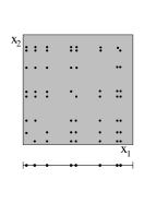
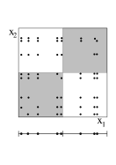
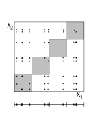
(a)                          (b)                          (c)                          (d)

Figure 1: Representation of a single event in $\Omega$ (shown as dots on the lines below the square) and in $\Omega\otimes\Omega$ space (in the squares). (a)–(c): Domains of box moments as a function of scale, (d): corresponding correlation integral domains. Filling in the “missing dots” along the diagonals would change factorial to ordinary moments.

While higher orders $q{>}2$ are not visualised as easily, their analysis proceeds analogously. Issues of “topology”, i.e. the combination of pairwise interparticle distances used to determine $q$-tuple size, come into play [3, 12].

Basing mathematical analysis on eventwise measures was instrumental in deriving correlation integral prescriptions for a HEP context [12] and in providing a mathematical basis for event mixing, whereby the uncorrelated background is simulated by analysing artificial events made up of particles selected randomly from different events in the sample.

Cumulants: The availability of large samples of low-multiplicity events led to the direct measure of cumulants, $\kappa_{q}$ [13] which have proven to be central to later experimental efforts due to their statistical properties and sensitivity. Their general properties include:

• Cumulants are zero when there is no net correlation.

• Cumulants of the sum of independent random variables $\mathbf{x}_{i}$ are additive,

  $$\kappa_{q}\bigl{(}\,{\textstyle\sum_{i}}\mathbf{x}_{i}\,\bigr{)}=\sum_{i}\kappa_{q}(\mathbf{x}_{i})\qquad q=1,2,3,\ldots$$ (2)

• The cumulant $\kappa_{q}(A-B)$ of distribution $A$ relative to distribution $B$ is equal to the difference of the $A$- and $B$-distribution cumulants [14],

  $$\kappa_{q}(A-B)=\kappa_{q}(A)-\kappa_{q}(B)\,.$$ (3)

  $B$ may, for example, be a reference distribution and $\kappa_{q}(A-B)$ the measured deviations from this pre-defined reference.

• With the exception of $\kappa_{1}$, multivariate cumulants are tensors under affine transformations; a simple example is $\kappa_{q}(c\mathbf{x})=c^{q}\,\kappa_{q}(\mathbf{x})$.

• Using event mixing, cumulants can be calculated even for correlation integrals [12].

An example of the usefulness of cumulants is shown in Fig. 2: measured second order cumulants for hadron-hadron collisions were fitted using various parametrisations (only the power law does well), and the same parametrisation then compared to measured third-order cumulants [15]. The discrepancy shows that the underlying model assumptions fail on third order even while being successful for $q{=}2$.

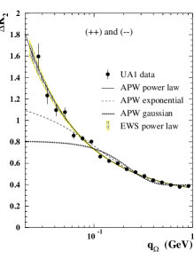
Figure 2: Use of cumulants in HEP to test theoretical models. Data was fitted to $q{=}2$ (left) and $q{=}3$ model predictions then compared to data (right).

Central Limit Theorem: Capitalising on the many particles generated in nucleus-nucleus collisions, recent experiments have exploited the close link between the scale $\ell$ of a region and the number $n$ of particles it can be expected to contain. Assume, simplistically, a constant number of particles $N$. Given the additivity property (2), it is easy to show that the cumulant of the average, $\langle x\rangle=N^{-1}\sum_{i=1}^{N}x_{i}$, is equal to the cumulant over a smaller region containing but one particle, suppressed by powers of $N$,

$$\kappa_{q}\left(\langle x\rangle\right)=N^{-q}\,\sum_{i}\kappa_{q}(x_{i})=N^{1-q}\,\kappa_{q}(x)\,,$$ (4)

if the $x_{i}$ are independent. Sensitive testing of independence is therefore provided by measuring the deviation from zero of the statistic

$$N^{q-1}\kappa_{q}\left(\langle x\rangle\right)-\kappa_{q}(x)\,.$$ (5)

while varying the scale interval over which $\langle x\rangle$ is calculated. This can be interpreted as an application of Eq. (3).

A more sophisticated version of this has recently been used [16] to partially address fluctuations in total eventwise multiplicity also: With $p(m)=\sum_{i=1}^{n_{m}}p_{i}$ the sum of all $n_{m}$ transverse momenta $p_{i}$ of particles found in bin $m$ of size $\ell$ for one event $e$, and $\overline{p}$ the average over momenta of particles from all events (“inclusive average”) in the same bin, the total variance, defined as

$$\Sigma_{p,n}^{2}(\ell)=\overline{\sum_{m}\left(p(m)-n_{m}\overline{p}\right)^{2}}\,,$$ (6)

turns out to be a difference between a $q{=}2$ cumulant over bins at scale $\ell$ and a cumulant at the smallest available scale, thereby effectively making use of Eq. (3). Multiplicity fluctuations are suppressed in Eq. (6) because $\Sigma^{2}_{p,n}$ is based on bin-averaged versions of the standardised variable $x^{*}=[x-\kappa_{1}(x)]/[\kappa_{2}(x)]^{1/2}$ which automatically subtracts out mean multiplicity $\kappa_{1}$.

Fig. 3 shows schematically how $\Sigma^{2}_{p,n}$ can be expected to behave as a function of scale $\ell\equiv\delta x$ [17]. Correlations manifest themselves as significant changes in $\Sigma^{2}_{p,n}$ with a change in scale, while lack of correlation shows up as invariance under change of measuring scale, which is another formulation of the Central Limit Theorem (CLT).

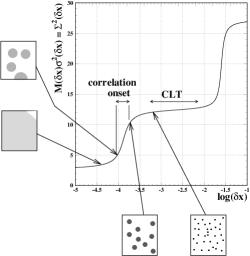
Figure 3: Changes with scale in correlation structure of “points” (shown under various magnifications in the little squares). Scale intervals of constant $\Sigma^{2}$ signify no correlation [17].

Other applications of cumulant differences include calculating cumulants for a fixed-multiplicity sample using the multinomial as reference distribution $B$ [14], and the calculation of quantum mechanical interference effects between the jets resulting from the weakly interacting bosons $W^{+}$ and $W^{-}$ [18].

Event-by-event physics: The availability of large samples allows the study of very detailed special cases or events. Selecting subsamples or plotting relative frequencies of events as a function of some event property has become known as “Event-by-event analysis”. Some have attempted to characterise individual events, for example by wavelet transforms [19], but so far, true event-by-event analysis has been rare. Nevertheless, the degrees of freedom provided by the sampling hierarchy [20] of particles, events, sampling distributions, special selections etc. are only just beginning to be appreciated and exploited.

Acknowledgments: The author thanks the organisers for a well-organised and stimulating workshop. This work was supported in part by the South African National Research Foundation.

References

- [1] P. Cvitanović, Physica A288, 61 (2000); nlin.CD/0001034.
- [2] T.S. Biro, C. Gong, B. Müller and A. Trayanov, Int. J. Mod. Phys. C5, 113 (1994), nucl-th/9306002.
-
[3]
P. Grassberger and I. Procaccia,
Phys. Rev. Lett. 50, 346 (1983);
P. Grassberger, Phys. Lett. A97, 227 (1983). - [4] T.C. Halsey, M.H. Jensen, L.P. Kadanoff, I. Procaccia and B.I. Shraiman, Phys. Rev. A33, 1141 (1986).
- [5] A. Rényi, Probability Theory, North Holland (1970).
- [6] E.A. de Wolf, I.M. Dremin and W. Kittel, Phys. Rep. 270, 1 (1996); M. Ploszajczak and R. Botet, Universal Fluctuations: the phenomenology of hadronic matter, World Scientific (2002).
- [7] Y. Wu and L. Liu, Phys. Rev. Lett. 70, 3197 (1993).
- [8] C.J.G. Evertsz and B.B. Mandelbrot, in: Chaos and Fractals, H.O. Peitgen, H. Jürgens and D. Saupe, Springer (1992).
- [9] A. Białas and R. Peschanski, Nucl. Phys. B273, 703 (1986).
- [10] P. Lipa and B. Buschbeck, Phys. Lett. B223, 465 (1989); P. Lipa, U. of Vienna PhD dissertation (1990) (unpublished).
- [11] L. Foà, Phys. Rep. 22, 1 (1975).
- [12] H.C. Eggers, P. Lipa, P. Carruthers and B. Buschbeck, Phys. Rev. D48, 2040 (1993).
- [13] A. Stuart and J.K. Ord, Kendall’s Advanced Theory of Statistics, Vol.1, Oxford University Press (1987).
- [14] P. Lipa, H.C. Eggers and B. Buschbeck, Phys. Rev. D53, R4711 (1996).
- [15] H.C. Eggers, P. Lipa, P. Carruthers, B. Buschbeck, Phys. Rev. Lett. 79, 197 (1997).
- [16] STAR Collaboration, J. Adams et al., nucl-ex/0308033.
- [17] T.A. Trainor, hep-ph/0001148.
- [18] L3 Collaboration, P. Achard et al., Phys. Lett. B547, 139 (2002).
- [19] I.M. Dremin et al., Phys. Lett. B499,97 (2001); hep-ph/0007060.
-
[20]
H.C. Eggers,
in: 30th International Symposium on
Multiparticle Dynamics, Tihany, Hungary, 9–15 October
2000, World Scientific (2001), pp. 291–302;
hep-ex/0102005.