Transversity and its accompanying T-odd distribution from Drell-Yan processes with pion-proton collisions
A. Sissakian, O. Shevchenko, A. Nagaytsev, O. Denisov,O. Ivanov
Joint Institute for Nuclear Research, 141980 Dubna, Russia

Abstract

It is studied the possibility of direct extraction of the transversity and its accompanying T-odd parton distribution function (PDF) from Drell-Yan (DY) processes with unpolarized pion beam and with both unpolarized and transversely polarized proton targets. At present, such a measurement can be performed on the COMPASS experiment at CERN. The preliminary estimations performed for COMPASS kinematic region demonstrate that it is quite real to extract both transversity and its accompanying T-odd PDF in the COMPASS conditions.

The advantage of DY process for extraction of PDFs, is that there is no need in any fragmentation functions. It is well known that the double transversely polarized DY process $H_{1}^{\uparrow}H_{2}^{\uparrow}\to l^{+}l^{-}X$ allows to directly extract the transversity distributions (see Ref. [1] for review). In particular, the double polarized DY process with antiproton beam is planned to be studied at PAX [2]. However, this is a rather difficult task to produce antiproton beam with the sufficiently high degree of polarization. So, it is certainly desirable to have an alternative (complementary) possibility allowing to extract the transversity PDF from unpolarized and single-polarized DY processes. This could be a matter of especial interest for the COMPASS experiment [3] where the possibility to study DY processes with unpolarized pion beam and with both unpolarized and transversely polarized proton targets $\pi^{-}p\rightarrow\mu^{+}\mu^{-}X$, $\pi^{-}p^{\uparrow}\rightarrow\mu^{+}\mu^{-}X$ is under discussion now.

The original expressions for unpolarized and single-polarized DY cross-sections [4] are very inconvenient in application since all $k_{T}$-dependent PDFs enter there in the complex convolution. To avoid this problem in Ref. [5] the $q_{T}$ integration approach [6, 7, 8] was applied. As a result, the procedure proposed in Ref. [5] allows to extract the transversity $h_{1}$ and the first moment

$$h_{1q}^{\perp(1)}(x)\equiv\int d^{2}{\bf k}_{T}\left(\frac{{\bf k}_{T}^{2}}{2M_{\pi}^{2}}\right)h_{1q}^{\perp}(x_{\pi},{\bf k}_{T}^{2})$$ (1)

of T-odd distribution $h_{1}^{\perp}$ directly, without any model assumptions about $k_{T}$-dependence of $h_{1}^{\perp}(x,k_{T}^{2})$.

The general procedure proposed in Ref. [5] applied to unpolarized DY process $\pi^{-}p\rightarrow\mu^{+}\mu^{-}X$ gives

$$\hat{k}{\Bigl{|}}_{\pi^{-}p\rightarrow\mu^{+}\mu^{-}X}=8\frac{\sum_{q}e_{q}^{2}[\bar{h}_{1q}^{\perp(1)}(x_{\pi}){\Bigl{|}}_{\pi^{-}}h_{1q}^{\perp(1)}(x_{p}){\Bigl{|}}_{p}+(x_{\pi}\leftrightarrow x_{p})]}{\sum_{q}e_{q}^{2}[\bar{f}_{1q}(x_{\pi}){\Bigl{|}}_{\pi^{-}}f_{1q}(x_{p}){\Bigl{|}}_{p}+(x_{\pi}\leftrightarrow x_{p})]},$$ (2)

where $\hat{k}$ is the coefficient at $\cos 2\phi$ dependent part of the properly integrated over $q_{T}$ ratio of unpolarized cross-sections:

$$\hat{R}=\frac{\int d^{2}{\bf q}_{T}[{\bf|}{\bf q}_{T}{\bf|}^{2}/{M_{\pi}M_{p}}][d\sigma^{(0)}/d\Omega]}{\int d^{2}{\bf q}_{T}\sigma^{(0)}},$$ (3)

$$\hat{R}=\frac{3}{16\pi}(\gamma(1+\cos^{2}\theta)+\hat{k}\cos 2\phi\sin^{2}\theta).$$ (4)

At the same time in the case of single polarized DY process $\pi^{-}p^{\uparrow}\rightarrow\mu^{+}\mu^{-}X$, operating just as in Ref. [5], one gets

$$\hat{A}_{h} = -\frac{1}{2}\frac{\sum_{q}e_{q}^{2}[\bar{h}_{1q}^{\perp(1)}(x_{\pi})h_{1q}(x_{p})+(x_{\pi}\leftrightarrow x_{p})]}{\sum_{q}e_{q}^{2}[\bar{f}_{1q}(x_{\pi})f_{1q}(x_{p})+(x_{\pi}\leftrightarrow x_{p})]},$$ (5)

where the single spin asymmetry (SSA) $\hat{A}_{h}$ is defined as

$$\hat{A}_{h}=\frac{\int d\Omega d\phi_{S_{2}}\int d^{2}{\bf q}_{T}(|{\bf q}_{T}|/M_{\pi})\sin(\phi+\phi_{S_{2}})[d\sigma({\bf S}_{2T})-d\sigma(-{\bf S}_{2T})]}{\int d\Omega d\phi_{S_{2}}\int d^{2}{\bf q}_{T}[d\sigma({\bf S}_{2T})+d\sigma(-{\bf S}_{2T})]}.$$ (6)

In Eqs. (2-6) the quantity $h_{1q}^{\perp(1)}(x_{\pi})$ is defined by Eq. (1). All other notations are the same as in Ref. [5] (see Ref. [1] for details on kinematics in the Collins-Soper frame we deal with).

Neglecting strange quark PDF contributions, squared sea contributions of $u$-quark PDF $h_{1u}^{\perp(1)}(x_{\pi}){\Bigl{|}}_{\pi^{-}}\bar{h}_{1u}^{\perp(1)}(x_{p}){\Bigl{|}}_{p}$, $f_{1u}(x_{\pi}){\Bigl{|}}_{\pi^{-}}\bar{f}_{1u}(x_{p}){\Bigl{|}}_{p}$, and cross terms containing the products of sea and valence $d$-quark PDFs (additionally suppressed by the charge factor $1/4$), one arrives at the simplified equations

$$\hat{k}(x_{\pi},x_{p}){\Bigl{|}}_{\pi^{-}p}\simeq 8\frac{\bar{h}_{1u}^{\perp(1)}(x_{\pi}){\Bigl{|}}_{\pi^{-}}h_{1u}^{\perp(1)}(x_{p}){\Bigl{|}}_{p}}{\bar{f}_{1u}(x_{\pi}){\Bigl{|}}_{\pi^{-}}f_{1u}(x_{p}){\Bigl{|}}_{p}},$$ (7)

$$\hat{A}_{h}(x_{\pi},x_{p}){\Bigl{|}}_{\pi^{-}p^{\uparrow}}\simeq-\frac{1}{2}\frac{\bar{h}_{1u}^{\perp(1)}(x_{\pi}){\Bigl{|}}_{\pi^{-}}h_{1u}(x_{p}){\Bigl{|}}_{p}}{\bar{f}_{1u}(x_{\pi}){\Bigl{|}}_{\pi^{-}}f_{1u}(x_{p}){\Bigl{|}}_{p}}.$$ (8)

Notice that while two equations corresponding to unpolarized and single-polarized antiproton-proton DY processes completely determine the transversity and its accompanying T-odd PDF in proton [5], two Eqs. (7) and (8) contain three unknown quantities $\bar{h}_{1u}^{\perp(1)}(x_{\pi}){\Bigl{|}}_{\pi^{-}}$, $h_{1u}^{\perp(1)}(x_{p}){\Bigl{|}}_{p}$ and $h_{1u}(x_{p})$. Nevertheless, from Eqs. (7) and (8) it immediately follows that

$$\frac{h_{1u}^{\perp(1)}(x_{p}){\Bigl{|}}_{p}}{h_{1u}(x_{p}){\Bigl{|}}_{p}}=-\frac{1}{16}\frac{\hat{k}(x_{\pi},x_{p}){\Bigl{|}}_{\pi^{-}p}}{\hat{A}_{h}(x_{\pi},x_{p}){\Bigl{|}}_{\pi^{-}p^{\uparrow}}}$$ (9)

Thus, using only unpolarized pion beam colliding with unpolarized and transversely polarized protons, it is possible to extract the ratio ${h_{1u}^{\perp(1)}(x_{p}){\Bigl{|}}_{p}}\,/\,{h_{1u}(x_{p}){\Bigl{|}}_{p}}$. However, it is certainly desirable to extract ${h_{1u}^{\perp(1)}(x_{p}){\Bigl{|}}_{p}}$ and ${h_{1u}(x_{p}){\Bigl{|}}_{p}}$ in separation.

The simplest way to solve this problem is to use in Eqs. (7), (8) the quantity $h_{1u}^{\perp(1)}{\Bigl{|}}_{p}$ extracted from $\hat{k}$ measured in unpolarized DY process, $\bar{p}p\rightarrow l^{+}l^{-}X$ (in the way proposed in Ref. [5]). However, if one wishes to extract all quantities within the experiment with the pion beam (COMPASS here) the additional assumptions connecting pion and proton PDFs are necessary. Taking into account the probability interpretations of $h_{1q}^{\perp}$ and $f_{1q}$ PDFs, it is natural to write the relation

$$\frac{\bar{h}_{1u}^{\perp(1)}(x){\Bigl{|}}_{\pi^{-}}}{h_{1u}^{\perp(1)}(x){\Bigl{|}}_{p}}=C_{u}\frac{\bar{f}_{1u}(x){\Bigl{|}}_{\pi^{-}}}{f_{1u}(x){\Bigl{|}}_{p}}.$$ (10)

Notice that the assumption given by Eq. (10) is in accordance (but is much less strong restriction) with the Boer’s model (see Eq. (50) in Ref. [4]), where $C_{u}=M_{p}c^{u}_{\pi}/M_{\pi}c^{u}_{p}$.

As we will see below, one should put $C_{u}$ to be about unity

$$C_{u}\simeq 1$$ (11)

to reconcile the results on $h_{1u}^{\perp(1)}$ in proton obtained from the simulated $\hat{k}{\Bigl{|}}_{\pi^{-}p}$ with the respective results [5] obtained from the simulated $\hat{k}{\Bigl{|}}_{\bar{p}p}$ as well as with the upper bound [5] on this quantity.

Thus, Eqs. (7) and (8) are rewritten as (c.f. Eqs. (19), (20) in Ref. [5])

$$\hat{k}(x_{\pi},x_{p}){\Bigl{|}}_{\pi^{-}p}\simeq 8\frac{h_{1u}^{\perp(1)}(x_{\pi}){\Bigl{|}}_{p}h_{1u}^{\perp(1)}(x_{p}){\Bigl{|}}_{p}}{f_{1u}(x_{\pi}){\Bigl{|}}_{p}f_{1u}(x_{p}){\Bigl{|}}_{p}}$$ (12)

$$\hat{A}_{h}(x_{\pi},x_{p}){\Bigl{|}}_{\pi^{-}p^{\uparrow}}\simeq-\frac{1}{2}\frac{h_{1u}^{\perp(1)}(x_{\pi}){\Bigl{|}}_{p}h_{1u}(x_{p}){\Bigl{|}}_{p}}{f_{1u}(x_{\pi}){\Bigl{|}}_{p}f_{1u}(x_{p}){\Bigl{|}}_{p}}.$$ (13)

Looking at Eqs. (12), (13), one can see that now the number of equations is equal to the number of variables to be found. Measuring the quantity $\hat{k}$ in unpolarized DY (Eqs. (3), (4)) and using Eq. (12) one can obtain the quantity $h_{1u}^{\perp(1)}{\Bigl{|}}_{p}$. Then, measuring SSA, Eq. (6), and using in Eq. (13) the obtained from unpolarized DY quantity $h_{1u}^{\perp(1)}{\Bigl{|}}_{p}$, one can eventually extract the transversity distribution $h_{1u}{\Bigl{|}}_{p}$.

To deal with Eqs. (12) and (13) in practice, one should consider them at the points $x_{\pi}=x_{p}\equiv x$ (i.e., $x_{F}\equiv x_{\pi}-x_{p}=0$), so that

$$h^{\perp(1)}_{1u}(x)=f_{1u}(x)\sqrt{\frac{\hat{k}(x,x){\Bigl{|}}_{\pi^{-}p}}{8}},$$ (14)

and

$$h_{1u}(x)=-4\sqrt{2}\frac{\hat{A}_{h}(x,x){\Bigl{|}}_{\pi^{-}p^{\uparrow}}}{\sqrt{\hat{k}(x,x){\Bigl{|}}_{\pi^{-}p}}}f_{1u}(x),$$ (15)

where now all PDFs refer to proton.

Figure 1: $\hat{k}$ versus $x_{\pi}$ for $x_{F}\simeq 0$. Data is obtained with MC simulations for 60 GeV (closed circles) and 100 GeV (open circles) pion beams.

To estimate the possibility of $h_{1u}^{\perp(1)}$ measurement, the special simulation of unpolarized DY events with the COMPASS kinematics are performed. The pion-proton collisions are simulated with the PYTHIA generator [10]. Two samples are prepared corresponding to 60 GeV and 100 GeV pion beams. Each sample contains about 100 K pure Drell-Yan events. The events are weighted (see Ref. [5] for detail) with the ratio of DY cross-sections given by (see Refs. [4, 11])

$$R\equiv\frac{d\sigma^{(0)}/d\Omega}{\sigma^{(0)}},$$ (16)

$$R=\frac{3}{16\pi}(1+\cos^{2}\theta+(\nu/2)\cos 2\phi\sin^{2}\theta)\quad(\nu\equiv 2\kappa),$$ (17)

where $\nu$ dependencies of $q_{T}$ and $x_{\pi}$ are taken from Refs. [11, 12].

Figure 2: $h_{1u}^{\perp(1)}$ versus $x_{\pi}$ for $x_{F}\simeq 0$. Data is obtained with MC simulations for 60 GeV (closed circles) and 100 GeV (open circles) pion beams.

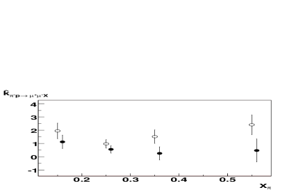
The angular distributions of $\hat{R}$ (Eqs. (3) and (4)) for both samples are studied just as it was done in Ref. [11] with respect to $R$ (Eqs. (16), (17)). The results are shown in Fig. 1. The value of $\hat{k}$ at averaged Q² for both energies are found to be $0.7\pm 0.1$ for 60 GeV and $0.9\pm 0.1$ for 100 GeV pion beams.

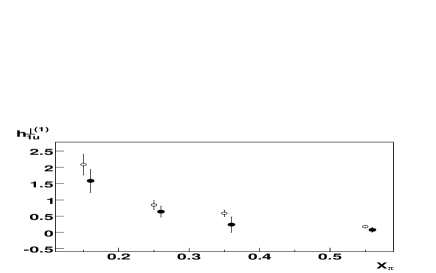
The quantity $h_{1u}^{\perp(1)}$ is reconstructed from the obtained values of $\hat{k}$ using Eq. (14) with $x_{F}=0\pm 0.04$. The results are shown in Fig. 2. Let us recall that to obtain $h_{1u}^{\perp(1)}$ from $\hat{k}{\Bigl{|}}_{\pi^{-}p}$, we chosen $C_{u}\simeq 1$. Notice that namely this choice of $C_{u}$ is consistent with the results on $h_{1u}^{\perp(1)}$ obtained in Ref. [5] from simulated $\hat{k}{\Bigl{|}}_{\bar{p}p}$ (compare Fig. 2 with Fig. 4 of Ref. [5]), and also with the upper bound on $h_{1u}^{\perp(1)}$ estimated in that paper. Otherwise, if $C_{u}$ essentially differs from unity, one should multiply the results on $h_{1u}^{\perp(1)}$ by the factor $1/\sqrt{C_{u}}$, that would lead to disagreement of the results on $h_{1u}^{\perp(1)}$ obtained from the simulated quantities $\hat{k}{\Bigl{|}}_{\pi^{-}p}$ and $\hat{k}{\Bigl{|}}_{\bar{p}p}$.

Certainly, all conclusions made on the basis of simulations are very preliminary. The reliable conclusion about $C_{u}$ can be made only from the future measurements of $\hat{k}$ for both DY processes with $\bar{p}$ and $\pi^{-}$ participation.

Figure 3: SSA given by Eq. (13) versus $x_{F}$ for 100 GeV pion beam ($Q^{2}_{average}=6.2\,GeV^{2}$).

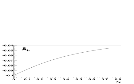
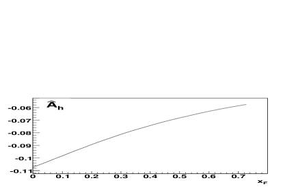
Using the obtained magnitudes of $h_{1u}^{\perp(1)}$ we estimate the expected SSA given by Eq. (13). The results are shown in Figs. 3 and 4. For estimation of $h_{1u}$ entering SSA together with $h_{1u}^{\perp(1)}$ (see Eq. (13)) we follow the procedure of Ref. [13] and use (rather crude) “evolution model” [1, 13] , where there is no any estimations of uncertainties. That is why in (purely qualitative) figures 3 and 4 we present the solid curves instead of points with error bars. To obtain these curves we reproduce $x$-dependence of $h_{1u}^{\perp(1)}$ in the considered region, using the Boer’s model (Eq. (50) in Ref. [4]), properly numerically corrected in accordance with the simulation results.

Figure 4: SSA given by Eq. (13) versus $x_{F}$ for 60 GeV pion beam ($Q^{2}_{average}=5.5\,GeV^{2}$).

It should be noticed that the estimations of $\hat{k}$ and $\hat{A}_{h}$ magnitudes obtained it this paper are very preliminary and show just the order of values of these quantities. For more precise estimations one needs the Monte-Carlo generator more suitable for DY processes studies (see, for example. Ref. [14] ) than PYTHIA generator which we used (with the proper weighting of events) here.

In summary, it is shown that the proposed in Ref. [5] procedure can be applied to DY processes: $\pi^{-}p\to\ \mu^{+}\mu^{-}X$ and $\pi^{-}p^{\uparrow}\to\ \mu^{+}\mu^{-}X$, which could be studied in the COMPASS experiment at CERN. The preliminary estimations for COMPASS kinematical region show the possibility to measure both $\hat{k}$ and SSA $\hat{A}_{h}$ and then to extract the quantities $h_{1}^{\perp(1)}$ and $h_{1}$ we are interesting in.

The authors are grateful to M. Anselmino, F. Balestra, R. Bertini, M.P. Bussa, A. Efremov, L. Ferrero, V. Frolov, T. Iwata, V. Krivokhizhin, A. Kulikov, P. Lenisa, A. Maggiora, A. Olshevsky, D. Panzieri, G. Piragino, G. Pontecorvo, I. Savin, M. Tabidze, O. Teryaev, W. Vogelsang and also to all members of Compass-Torino group for fruitful discussions. The work of O.S. and O.I. was supported by the Russian Foundation for Basic Research (project no. 05-02-17748).

References

- [1] V. Barone, A. Drago, and P.G. Ratcliffe, Phys. Rep. 359, 1 (2002).
- [2] V. Barone et. al (PAX collaboration), hep-ex/0505054
- [3] G.K.Mallot, Nucl. Inst. Meth. A518 (2004) 121.
- [4] D. Boer, Phys. Rev. D60, 014012 (1999).
- [5] A.N. Sissakian, O.Yu. Shevchenko, A.P. Nagaytsev, O.N. Ivanov, Phys. Rev. D72 (2005) 054027
- [6] D. Boer, R. Jakob, P. J. Mulders, Nucl. Phys. B 504, 345 (1997)
- [7] D. Boer, R. Jakob, P. J. Mulders, Phys. Lett. B 424, 143 (1998)
- [8] D. Boer, P. J. Mulders, Phys. Rev. D 57, 5780 (1998)
- [9] A.V. Efremov et al, Phys. Lett. B 612, 233 (2005).
- [10] T. Sjostrand et al., hep-ph/0308153.
- [11] J.S. Conway et al, Phys. Rev. D39, 92 (1989).
- [12] NA10 Collab., Z. Phys. C31, 513 (1986); Z. Phys. C37, 545 (1988).
- [13] M. Anselmino, V. Barone, A. Drago, N.N. Nikolaev, Phys.Lett. B594, 97 (2004).
- [14] A. Bianconi, M. Radici Phys. Rev. D 71, 074014 (2005).