PHENOMENOLOGICAL AND COSMOLOGICAL ASPECTS OF A MINIMAL GUT SCENARIO

Abstract

Several phenomenological and cosmological aspects of a minimal extension of the Georgi-Glashow model, where the Higgs sector is composed by $\bm{5}_{H}$, $\bm{15}_{H}$, and $\bm{24}_{H}$, are studied. It is shown that the constraints coming from the unification of gauge interactions up to two-loop level predict light scalar leptoquarks. In this GUT scenario, the upper bound on the total proton decay lifetime is $\tau_{p}\leq 1.4\times 10^{36}$ years. The possibility to explain the matter-antimatter asymmetry in the universe through the decays of $SU(2)_{L}$ scalar triplets is also studied. We find that a successful triplet seesaw leptogenesis implies an upper bound on the scalar leptoquark mass, $M_{\Phi_{b}}\lesssim 10^{6-7}$ GeV. We conclude that this GUT scenario can be tested at the next generation of proton decay experiments and future colliders through the production of scalar leptoquarks.

I Introduction

Grand unified theories (GUTs) based on the $SO(10)$ gauge symmetry SO(10)1 ; Fritzsch:1974nn are usually considered as the most appealing candidates for the unification of electroweak and strong interactions. They offer a number of advantages over $SU(5)$ theories GG : (i) They provide a natural explanation of the smallness of neutrino masses through the seesaw mechanism seesaw ; (ii) they accommodate all fermions of one generation into one representation; (iii) they represent, in their minimal form, the most promising theory of fermion masses (For realistic grand unified theories based on the $SO(10)$ gauge symmetry see e.g. Refs. Babu:1998wi ; Aulakh:2003kg ; Babu:2005gx .).

Nevertheless, it is well known that the only promising way to test the idea of grand unification is through nucleon decay. Therefore, it is very important to investigate the simplest realistic grand unified theory where proton decay can be well predicted. This crucial issue brings us back to non-supersymmetric GUT scenarios, since the unification scale is rather low $(M_{GUT}\approx 10^{14}~{}\textrm{GeV})$. In particular, we focus on the simplest realistic $SU(5)$ theories, where the unification scale can be accurately predicted. Even though $SU(5)$ possesses uncorrelated regions in the Yukawa sector, the simplicity of the Higgs sector in the non-supersymmetric case offers a hope that the theory can be verified in near future.

In a recent work Dorsner:2005fq , some of us argued that the simplest realistic extension of the Georgi-Glashow (GG) model is the one containing the $\bm{5}_{H}$, $\bm{15}_{H}$ and $\bm{24}_{H}$ representations in the Higgs sector. The purpose of this paper is to demonstrate that the next generation of collider and proton decay experiments will refute or verify this minimal $SU(5)$ scenario. A first attempt was made in Ref. Dorsner:2005fq in this direction. Here we offer the full two-loop treatment of the gauge coupling unification and discuss the constraints on the Higgs sector. To show the testability of the model, we include all the presently available experimental limits in our discussion. The upper bound on the total proton decay lifetime in our GUT model is corrected, and we investigate the possibility to explain the baryon asymmetry observed in the universe through the decays of $SU(2)_{L}$ scalar triplets living in $\bm{15}_{H}$, showing how important the constraints coming from leptogenesis turn out to be. The latter, when combined with the unification constraints, lead us to conclude that the present GUT scenario could be tested at the next generation of collider experiments through the production of light leptoquarks.

II A minimal $SU(5)$ scenario

Ever since its inception in 1974, the $SU(5)$ model of Georgi and Glashow GG has been considered as the minimal grand unified theory. It offers partial matter unification of one standard model (SM) family $a$ ($a=1,2,3$) in the anti-fundamental ${\bf\overline{5}}_{a}$ and antisymmetric ${\bf 10}_{a}$ representations. The GUT symmetry is broken down to the standard model by the vacuum expectation value (VEV) of the Higgs field in the $\bm{24}_{H}$, while the SM Higgs resides in the $\bm{5}_{H}$. The beauty of the model is undeniable, but the model itself is not realistic. Indeed, there are several problems some of which are correlated:

• Gauge coupling unification.

  The most dramatic problem of the naive $SU(5)$ is the lack of unification. Namely, using the whole freedom of the model, one can compute the maximum value of the ratio between the parameters $B_{23}=b_{2}-b_{3}$ and $B_{12}=b_{1}-b_{2}$, where $b_{i}$ ($i=1,2,3$) are the beta functions of the particle content of the theory for $U(1)_{Y}$, $SU(2)_{L}$ and $SU(3)_{C}$, respectively. One gets $B_{23}^{SU(5)}/B_{12}^{SU(5)}\leq 0.60$, while the present experimental data requires $B_{23}/B_{12}=0.719\pm 0.005$.

• Relation between Yukawa couplings of quarks and leptons.

  A second major problem is related to the predicted relation $Y_{D}=Y_{E}^{T}$ between the down quark and charged lepton Yukawa coupling matrices. This prediction is in strong disagreement with the experiment, especially in the case of the first and second generations of fermions. There are two solutions to this issue: one can add higher-dimensional operators Ellis:1979fg or introduce the ${\bf 45_{H}}$ representation Georgi:1979df .

• Neutrino masses.

  In the Georgi-Glashow model, neutrinos are massless. However, today we know that they do have a tiny mass. Therefore, the model has to be extended in order to account for non-vanishing neutrino masses. There are two possible solutions: one can introduce at least two right-handed neutrinos and use the so-called Type I seesaw mechanism seesaw , or one can add the representation ${\bf 15}_{H}$ in order to generate neutrino masses through the Type II seesaw mechanism TypeII .

• Doublet-triplet (DT) splitting problem.

  Another problem in the naive $SU(5)$ is that it cannot explain why the Higgs doublet living in ${\bf 5}_{H}$ is light. Although there are no solutions to this issue in the context of a non-supersymmetric scenario, different mechanisms are conceivable in SUSY $SU(5)$ to achieve the splitting between the triplet and the doublet. (See for example Ref. Berezhiani:1997as for a review.)

The simplest way Dorsner:2005fq to address the first three problems listed above in a non-supersymmetric framework consists of extending the minimal GG model with the ${\bf 15}_{H}$ and allowing for higher-dimensional operators. More precisely, the Higgs sector is $\bm{24}_{H}=\Sigma=(\Sigma_{8},\Sigma_{3},\Sigma_{(3,2)},\Sigma_{(\bar{3},2)},\Sigma_{24})=(\bm{8},\bm{1},0)+(\bm{1},\bm{3},0)+(\bm{3},\bm{2},-5/6)+(\overline{\bm{3}},\bm{2},5/6)+(\bm{1},\bm{1},0)$, $\bm{15}_{H}=\Phi=(\Phi_{a},\Phi_{b},\Phi_{c})=(\bm{1},\bm{3},1)+(\bm{3},\bm{2},1/6)+(\bm{6},\bm{1},-2/3)$, $\bm{5}_{H}=\Psi=(\Psi_{D},\Psi_{T})=(\bm{1},\bm{2},1/2)+(\bm{3},\bm{1},-1/3)$, where $\Sigma_{(3,2)}$ and $\Sigma_{(\bar{3},2)}$ are fields eaten by the superheavy gauge fields $V$. In what follows we define the GUT scale through their mass: $M_{GUT}=M_{V}$. As emphasized in Dorsner:2005fq , in this non-supersymmetric grand unified model, the GUT scale is low and can be predicted with great precision. This gives us the possibility to test the grand unification idea at future proton decay experiments. In fact, in our view, grand unified theories are the theories for the decay of the proton, since they provide us with the necessary input to compute the corresponding partial lifetimes. Of course, one can also think of other minimal extensions of grand unified theories based on higher groups. However, since in those models it is very difficult to predict the GUT scale and the masses of the superheavy gauge bosons mediating nucleon decay, the predictions for the lifetime of the proton are far from accurate.

In the GUT scenario proposed in Dorsner:2005fq the scalar potential reads as:

$$V\ = \ V_{SU(5)}^{\rm naive}\ +\ \overline{5}^{T}_{ai}\ C\ h^{ab}\ \overline{5}_{bj}\ 15_{H}^{ij}\ -\ \frac{\mu_{\Phi}^{2}}{2}\text{Tr}\,15_{H}^{\dagger}15_{H}\ +\ \frac{a_{\Phi}}{4}(\text{Tr}\,15_{H}^{\dagger}15_{H})^{2}$$ (1)

$$+ \frac{b_{\Phi}}{2}\,\text{Tr}\,(15_{H}^{\dagger}15_{H}15_{H}^{\dagger}15_{H})\ +\ c_{2}\,\text{Tr}\,(15_{H}^{\dagger}24_{H}15_{H})\ +\ c_{3}\ 5_{H}^{\dagger}\ 15_{H}\ 5_{H}^{*}$$

$$+ \ c_{3}^{*}\ 5_{H}^{T}\ 15_{H}^{\dagger}5_{H}\ +\ b_{1}\,\text{Tr}\,(15_{H}^{\dagger}15_{H})\text{Tr}\,24_{H}^{2}\ +\ b_{3}\ 5_{H}^{\dagger}5_{H}\,\text{Tr}\,(15_{H}^{\dagger}15_{H})\$$

$$+ \ b_{5}\ 5_{H}^{\dagger}15_{H}15_{H}^{\dagger}5_{H}\ +\ b_{6}\,\text{Tr}\,(15_{H}15_{H}^{*}24_{H}^{2})\ +\ b_{7}\,\text{Tr}\,(15_{H}^{*}24_{H}15_{H}24_{H}^{*})$$

$$+ \ b_{8}\ 5_{H}^{\dagger}24_{H}15_{H}5_{H}^{*}\ +\ b^{*}_{8}\ 5_{H}^{T}24_{H}15^{\dagger}_{H}5_{H}\ +\ \textrm{higher-dimensional terms},$$

where $V_{SU(5)}^{\rm naive}$ is the scalar potential of the Georgi-Glashow model.

III Unification

In this section we present the constraints that exact gauge coupling unification places on the masses of the scalars of the theory. We first present the one-loop level analysis to outline the basic features of the scalar mass spectrum and only then we resort to the more accurate two-loop analysis.

III.1 One-Loop Analysis

The one-loop level relations between the gauge couplings at $M_{Z}$ and the unifying gauge coupling $\alpha_{GUT}=g^{2}_{GUT}/(4\pi)$ at $M_{GUT}$ are

$$\left.\alpha^{-1}_{i}\right|_{M_{Z}}=\alpha^{-1}_{GUT}+\frac{b_{i}}{2\pi}\ln\frac{M_{GUT}}{M_{Z}},$$ (2)

where $i=1,2,3$ for $U(1)$, $SU(2)$, and $SU(3)$, respectively, and $b_{i}$ are the familiar one-loop $\beta$ function coefficients. The SM particle content with $n$ light Higgs doublet fields yields $b_{1}=40/10+n/10$, $b_{2}=-20/6+n/6$ and $b_{3}=-7$.

Eqs. (2) hold under the assumption that there is a particle “desert” between $M_{Z}$ and $M_{GUT}$. However, there is no particular reason that this should be the case. If there are $I$ particles with intermediate masses $M_{I}$ ($M_{Z}\leq M_{I}\leq M_{GUT}$), these equations remain unaltered except for the substitutions $b_{i}\rightarrow B_{i}$, where $B_{i}=b_{i}+\sum_{I}b_{iI}r_{I}$ are the so-called effective coefficients. Here $b_{iI}$ are the appropriate one-loop coefficients of the particle $I$ and $r_{I}=(\ln M_{GUT}/M_{I})/(\ln M_{GUT}/M_{Z})$ ($0\leq r_{I}\leq 1$) is its “running weight”.

The elimination of $\alpha_{GUT}$ from Eqs. (2) leaves the following two equations that connect the effective coefficients $B_{ij}=B_{i}-B_{j}$ with the low-energy observables Giveon:1991zm :

$$\frac{B_{23}}{B_{12}}=\frac{5}{8}\frac{\sin^{2}\theta_{W}-\alpha_{em}/\alpha_{s}}{3/8-\sin^{2}\theta_{W}}\,,\qquad\ln\frac{M_{GUT}}{M_{Z}}=\frac{16\pi}{5}\frac{3/8-\sin^{2}\theta_{W}}{\alpha_{em}B_{12}}\,.$$ (3)

Adopting the following experimental values at $M_{Z}$ in the $\overline{MS}$ scheme Eidelman:2004wy : $\sin^{2}\theta_{W}=0.23120\pm 0.00015$, $\alpha_{em}^{-1}=127.906\pm 0.019$ and $\alpha_{s}=0.1187\pm 0.002$, these read

$$\frac{B_{23}}{B_{12}} = 0.719\pm 0.005\,,$$ (4a)

$$\ln\frac{M_{GUT}}{M_{Z}} = \frac{184.9\pm 0.2}{B_{12}}\,.$$ (4b)

Eq. (4a) is sometimes referred to as the $B$-test. It basically shows whether unification takes place or not. Eq. (4b), on the other hand, could be referred to as the GUT scale relation since it yields the GUT scale value once Eq. (4a) is satisfied.

The $B$-test fails badly in the SM case ($B_{23}/B_{12}=0.53$), and hence the need for extra light particles with suitable $B_{ij}$ coefficients to bring the value of the $B_{23}/B_{12}$ ratio in agreement with its experimental value. In our case the presence of the $\bm{15}_{H}$ is essential. The $B_{ij}$ coefficients for all the particles in our scenario are presented in Table 1. Clearly, $\Sigma_{3}$, $\Phi_{a}$ and $\Phi_{b}$ improve unification with respect to the SM case, while $\Sigma_{8}$, $\Psi_{T}$ and $\Phi_{c}$ act in the opposite manner. We recall that we set $M_{V}=M_{GUT}$, where $M_{V}$ is the mass of the superheavy gauge bosons. We thus take $\Sigma_{8}$, $\Psi_{T}$ and $\Phi_{c}$ to reside at or above the GUT scale in our numerical analysis. We relax this assumption later to discuss its impact on our findings.

Table 1: $B_{ij}$ coefficients.

	Higgsless SM	$\Psi_{D}$	$\Psi_{T}$	$V$	$\Sigma_{8}$	$\Sigma_{3}$	$\Phi_{a}$	$\Phi_{b}$	$\Phi_{c}$
$B_{23}$	$\frac{11}{3}$	$\frac{1}{6}$	$-\frac{1}{6}r_{\Psi_{T}}$	$-\frac{7}{2}r_{V}$	$-\frac{1}{2}r_{\Sigma_{8}}$	$\frac{1}{3}r_{\Sigma_{3}}$	$\frac{2}{3}r_{\Phi_{a}}$	$\frac{1}{6}r_{\Phi_{b}}$	$-\frac{5}{6}r_{\Phi_{c}}$
$B_{12}$	$\frac{22}{3}$	$-\frac{1}{15}$	$\frac{1}{15}r_{\Psi_{T}}$	$-7r_{V}$	0	$-\frac{1}{3}r_{\Sigma_{3}}$	$-\frac{1}{15}r_{\Phi_{a}}$	$-\frac{7}{15}r_{\Phi_{b}}$	$\frac{8}{15}r_{\Phi_{c}}$

The value of $B_{12}$ determines the scale of unification through the GUT scale relation (4b). Therefore, a lower bound on $B_{12}$ translates into an absolute upper bound on the GUT scale. If we naively set $M_{\Sigma_{3}}=M_{\Phi_{a}}=M_{\Phi_{b}}=M_{Z}$ ($r_{\Sigma_{3}}=r_{\Phi_{a}}=r_{\Phi_{b}}=1$) we obtain $B_{12}>6.4$ and accordingly $M_{GUT}<3.2\times 10^{14}$ GeV. This constraint, when combined with the relation $M_{GUT}=M_{V}$, determines an upper bound on the proton lifetime, if the corresponding value of $\alpha_{GUT}$ is known. To find the latter we resort to the numerical analysis. However, the non-supersymmetric nature of our scenario suggests this value to be around $1/39$.

In the one-loop analysis we treat $M_{GUT}$, $M_{\Sigma_{3}}$, $M_{\Phi_{a}}$ and $M_{\Phi_{b}}$ as free parameters and investigate the possibility to find a consistent scenario with exact gauge coupling unification. Since we have four free parameters and two equations—Eqs. (4a) and (4b)—we opt to present the $M_{\Sigma_{3}}$ and $M_{\Phi_{a}}$ contours in the $M_{GUT}$–$M_{\Phi_{b}}$ plane in Fig. 1. The line of constant $\alpha^{-1}_{GUT}$ is also shown.

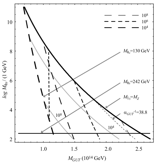
Figure 1: Plot of lines of constant $M_{\Sigma_{3}}$ and $M_{\Phi_{a}}$ in the $M_{GUT}$–$\textit{log}\,(M_{\Phi_{b}}/1\,\textrm{GeV})$ plane, assuming exact one-loop unification. We use the central values for the gauge couplings as given in the text. All the masses are given in GeV units. The triangular region is bounded from the left (below) by the experimental limit on $M_{\Phi_{a}}$ ($M_{\Phi_{b}}$). The right bound is $M_{\Sigma_{3}}\geq M_{Z}$. The two grey solid (thick dashed) lines are the lines of constant $M_{\Sigma_{3}}$ ($M_{\Phi_{a}}$). The line of constant $\alpha^{-1}_{GUT}\,$ is also shown. The region to the left of the vertical dashed line is excluded by the proton decay experiments if $\alpha=0.015$ GeV³.

The triangular region in Fig. 1 represents the available parameter space under the assumption that $\Psi_{T}$, $\Sigma_{8}$ and $\Phi_{c}$ reside at or above the GUT scale. The region is bounded from the left and below by the experimental limits on $M_{\Phi_{a}}$ and $M_{\Phi_{b}}$, respectively. (For the discussion on the origin of the experimental limits see Dorsner:2005fq and references therein.) The right bound stems from the requirement that $M_{\Sigma_{3}}\geq M_{Z}$. It is expected that the Large Hadron Collider (LHC) will place a more stringent lower limit on the mass of the scalar leptoquark $\Phi_{b}$ at around $1$ TeV (For experimental bounds on leptoquark masses see Refs. Leptoexperiments .).

Fig. 1 reveals that the masses of the three scalar fields that improve unification, namely, $\Sigma_{3}$, $\Phi_{a}$ and $\Phi_{b}$, have to be below the GUT scale. This, however, does not hold at two-loop level. The GUT scale is rather low and, for a given value of $\alpha_{GUT}$, the predicted value for the proton decay lifetime is within the reach of the present and future proton decay experiments. More precisely, if the nucleon matrix element is taken to be $\alpha=0.015$ GeV³, the region to the left of the vertical thick dashed line in Fig. 1 is already excluded by the present limits on the proton decay lifetime. In order to generate this bound we assume maximal flavor suppression of the gauge $d=6$ proton decay operators as explained in the next section in more details. Clearly, due to the simplicity of our scenario, experimental limits place firm upper bounds on $M_{\Sigma_{3}}$, $M_{\Phi_{a}}$ and $M_{\Phi_{b}}$.

What happens if we relax the $M_{\Psi_{T}},M_{\Sigma_{8}},M_{\Phi_{c}}\geq M_{GUT}$ assumption? If either $M_{\Psi_{T}}$ or $M_{\Phi_{c}}$ are below the GUT scale, then they both decrease $M_{GUT}$ due to an increase of the $B_{12}$ coefficient. They also change the $B_{23}/B_{12}$ ratio in the wrong direction, which has to be compensated by appropriate changes in the $\Sigma_{3}$, $\Phi_{a}$ and $\Phi_{b}$ contributions. Pictorially, as one lowers $M_{\Psi_{T}}$ and $M_{\Phi_{c}}$ the $M_{\Phi_{a}}=130$ GeV line in Fig. 1 moves very slowly to the left while, at the same time, $M_{\Sigma_{3}}=M_{Z}$ moves very rapidly in the same direction until the triangular region shrinks to a point. In other words, any scenario in which $M_{\Psi_{T}}$ or $M_{\Phi_{c}}$ or both are below the GUT scale would be more significantly exposed to the tests through the proton decay lifetime measurements and accelerator searches than the scenario shown in Fig. 1.

If, on the other hand, one lowers the mass of $\Sigma_{8}$, the $M_{\Phi_{a}}=130$ GeV line moves to the right more rapidly than the $M_{\Sigma_{3}}=M_{Z}$ line until the triangular region becomes a point when $M_{\Sigma_{8}}$ reaches $10^{5}$ GeV. At that point $M_{GUT}$ reaches the upper bound of $3.2\times 10^{14}$ GeV for $M_{\Sigma_{8}}=10^{5}$ GeV, $M_{\Sigma_{3}}=M_{Z}$, $M_{\Phi_{a}}=130$ GeV, $M_{\Phi_{b}}=242$ GeV and $\alpha_{GUT}^{-1}=37.3$. Again, the upper bound on the masses of $\Sigma_{3}$, $\Phi_{b}$ and $\Phi_{a}$ would be significantly lower as long as $M_{\Sigma_{8}}<M_{GUT}$.

III.2 Two-Loop Analysis

The simplicity of the Higgs sector allows us to repeat the same analysis at the two-loop level. We require exact unification and present the available parameter space in Fig. 2. In the two-loop analysis we must also take into account the one-loop running of the Yukawa couplings. The relevant input parameters at the $M_{Z}$ scale, such as the fermion masses and CKM angles that are used in the running are specified in Table I of Ref. Barr:2005ss . The stars in Fig. 2 represent points that correspond to exact unification.

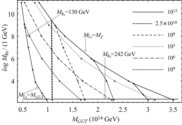
Figure 2: Unification of the gauge couplings at the two-loop level. Stars correspond to exact numerical two-loop unification solutions. There are two sets of lines of constant value. The steeper set is associated with $M_{\Phi_{a}}$ and the other one represents the lines of constant $M_{\Sigma_{3}}$. All the masses are in GeV units. The region to the left of the vertical dashed line is excluded by the proton decay experiments if $\alpha=0.015$ GeV³.

The upper bound on the GUT scale is shifted to a higher value (about a factor of $\sqrt{2}$) with respect to the one-loop case. There also appears a line along which $M_{\Sigma_{3}}$ is not required to be below $M_{GUT}$ to accomplish exact unification. Moreover, the allowed values of $M_{\Phi_{a}}$ are significantly larger than in the one-loop analysis. As before, by relaxing the assumption $M_{\Psi_{T}},M_{\Phi_{c}}\geq M_{GUT}$ ($M_{\Sigma_{3}}\geq M_{GUT}$), the allowed region moves to the left (right) and shrinks as we lower the relevant masses.

At two-loop level, the corrected upper bound on $M_{GUT}$ is $4.6\times 10^{14}$ GeV for $M_{\Sigma_{8}}=M_{Z}$, $M_{\Sigma_{3}}=M_{Z}$, $M_{\Phi_{a}}=6.4\times 10^{3}$ GeV, $M_{\Phi_{b}}=242$ GeV and $\alpha_{GUT}^{-1}=37.06$. We use these values in the next section to derive an accurate upper bound on the proton decay lifetime. If $\alpha=0.015$ GeV³ the proton decay lifetime measurements already exclude the part to the left of the thick dashed line ($M_{GUT}\gtrsim 1.1\times 10^{14}$ GeV) and establish a triangular region with the maximal value for $M_{\Phi_{b}}$ around $10^{9}$ GeV.

With the two-loop analysis at hand, we can finally answer the following question. How much improvement in the lifetime limits do proton decay experiments need in order to completely exclude our scenario? In the “worst” case scenario the two-loop GUT scale is approximately by a factor of four larger than the current proton decay bound presented in Fig. 2. Hence, an improvement in the measurements of proton lifetime by a factor of $4^{4}$ is called for to completely rule out this GUT scenario. The situation is actually much better than that, since even the slightest improvement in the proton lifetime bounds (by a factor of fifteen) will make our scenario incompatible with exact unification unless either $\Phi_{b}$ or $\Sigma_{3}$ resides below $10^{3}$ GeV, thus making them accessible in accelerator experiments.

III.3 $\Sigma\rightarrow-\Sigma$ Invariance

Fig. 2 shows that $\Sigma_{3}$ and $\Sigma_{8}$ are highly non-degenerate in some parts of the allowed parameter space. This, however, seems in conflict with the tree-level relation $M_{\Sigma_{3}}=4M_{\Sigma_{8}}$ of the $\Sigma$ potential, which is invariant under the $\Sigma\rightarrow-\Sigma$ transformation Buras . Since we commit to the scenario that includes all possible terms allowed by the gauge symmetry, we are forced to depart from this commonly used invariance. This has three important consequences: (i) the cubic term ($\text{Tr}\,\Sigma^{3}$) in the potential violates the validity of the $M_{\Sigma_{3}}=4M_{\Sigma_{8}}$ relation Guth ; (ii) the higher dimensional terms linear in $\Sigma/\Lambda$ in the Yukawa part of the Lagrangian allow for masses of quarks and leptons that are in agreement with the experimentally observed values ; (iii) a term linear in both $\Sigma$ and $\bm{15}_{H}$ appears in the scalar part of the potential that is relevant for both the proton decay and neutrino masses if $\bm{15}_{H}$ couples to matter fields.

To demonstrate how constraining the demand for $\Sigma\rightarrow-\Sigma\,$ invariance is, we present one example in a somewhat simpler setting. Recall the Georgi-Glashow $SU(5)$ model with two Higgs fields—one in the adjoint and the other in the fundamental representation. After imposing the $\Sigma\rightarrow-\Sigma$ invariance there are seven terms left in the scalar potential. It is easy to show Buras that once $\Sigma_{24}$ gets a VEV $v_{1}$ of the order of the GUT scale and $\Psi_{D}$ gets the electroweak scale VEV $v_{2}$, the electrically neutral component of $\Sigma_{3}$ must get a VEV of the order of $v_{3}\sim v_{2}^{2}/v_{1}$ (For the relevant equations and further discussion see MaLi . We note that there is a term $+\lambda_{4}v_{2}v_{3}^{2}$ missing on the right hand side of Eq. (11) of Ref. MaLi .) The above statement, however, is not necessarily correct if we include two more terms in the potential that are absent under the $\Sigma\rightarrow-\Sigma$ invariance. In other words, a classical solution with appropriate VEVs for $\Sigma_{24}$ and $\Psi_{D}$ but with no VEV for $\Sigma_{3}$ is allowed if the potential is not invariant under $\Sigma\rightarrow-\Sigma\,$.

We conclude this section with the following observation. In our analysis we include all the terms allowed by the underlying gauge symmetry. In this way we insure that the predictions of our scenario are independent of any particular set of assumptions. The benefit of such an approach is clear: if the predictions of our scenario are experimentally refuted, then the scenario is ruled out regardless of any particular assumptions.

IV Upper bound on the total proton decay lifetime

Proton decay is a generic prediction coming from matter unification. We thus believe this to be the most promising way to test the beautiful idea of grand unification. It is commonly thought that non-supersymmetric GUT scenarios are ruled out by the limits on nucleon decay lifetimes, since the unification scale is around $10^{14}$ GeV. This, however, holds only in GUT scenarios where the Yukawa sector is quite constrained. In general, this is no longer true because proton decay predictions are different for each model of fermion masses Dorsner:2004xa . To show that our minimal non-supersymmetric GUT scenario based on $SU(5)$ gauge group is not ruled out by such limits, we look for an upper bound on the total proton decay lifetime. For new experimental lower bounds on the partial lifetime of the proton see Ref. newbounds .

It is well known that in any non-supersymmetric scenario the most important contributions to the decay of the proton are the so-called gauge $d=6$ contributions. In the physical basis, these effective operators read as FileviezPerez:2004hn :

$$O(\nu_{l},d_{\alpha},d^{C}_{\beta}) = \frac{g_{GUT}^{2}}{2M_{V}^{2}}\ (V_{1}\ V_{UD})^{1\alpha}\ (V_{3}\ V_{EN})^{\beta l}\ \overline{u^{C}}\ \gamma^{\mu}\ L\ d_{\alpha}\ \overline{d^{C}_{\beta}}\ \gamma_{\mu}\ L\ \nu_{l}\,,$$ (5)

$$O(e^{C}_{\alpha},d_{\beta}) = \frac{g_{GUT}^{2}}{2M_{V}^{2}}\ \left(V_{1}^{11}\ V_{2}^{\alpha\beta}\ +\ (V_{1}\ V_{UD})^{1\beta}(V_{2}\ V_{UD}^{\dagger})^{\alpha 1}\right)\ \overline{u^{C}}\ \gamma^{\mu}\ L\ u\ \overline{e^{C}_{\alpha}}\ \gamma_{\mu}\ L\ d_{\beta}\,,$$ (6)

$$O(e_{\alpha},d^{C}_{\beta}) = \frac{g_{GUT}^{2}}{2M_{V}^{2}}\ V_{1}^{11}\ V_{3}^{\beta\alpha}\ \overline{u^{C}}\ \gamma^{\mu}\ L\ u\ \overline{d^{C}_{\beta}}\ \gamma_{\mu}\ L\ e_{\alpha}\,.$$ (7)

In the above equations $V_{1}=U_{C}^{\dagger}\,U$, $V_{2}=E_{C}^{\dagger}\,D$, $V_{3}=D_{C}^{\dagger}\,E$, $V_{4}=D_{C}^{\dagger}\,D$, $V_{UD}=U^{\dagger}\,D$, $V_{EN}=E^{\dagger}\,N$ are mixing matrices; $L=(1-\gamma_{5})/2$ and $\alpha,\beta=1,2$; $l=1,2,3$. Our convention for the diagonalization of the up, down, charged lepton and neutral lepton Yukawa matrices is specified by

$$U^{T}_{C}\ Y_{U}\ U=Y_{U}^{\textrm{diag}}\,,\quad D^{T}_{C}\ Y_{D}\ D=Y_{D}^{\textrm{diag}}\,,\quad E^{T}_{C}\ Y_{E}\ E=Y_{E}^{\textrm{diag}}\,,\quad N^{T}\ Y_{\nu}\ N=Y_{\nu}^{\textrm{diag}}\,.$$ (8)

The quark and leptonic mixing are given in our notation by $V_{UD}=U^{\dagger}D=K_{1}V_{CKM}K_{2}$ and $V_{EN}=K_{3}V_{PMNS}$, respectively, where $K_{1}$, $K_{3}$ and $K_{2}$ are diagonal matrices containing three and two phases, respectively.

The way to find an upper bound on the total proton decay lifetime by investigating the possible freedom in the Yukawa sector of grand unified theories has been pointed out in Ref. Dorsner:2004xa . For a given value of $\alpha_{GUT}$ and the super-heavy gauge boson mass, it has been shown that the upper bound in the case of Majorana neutrinos is given by Dorsner:2004xa :

$$\tau_{p}\leq\frac{6}{\alpha_{GUT}^{2}}\times\left(\frac{M_{V}}{10^{16}\textrm{GeV}}\right)^{4}\times\left(\frac{0.003\textrm{GeV}^{3}}{\alpha}\right)^{2}\ \times 10^{39}\ \textrm{years}\,.$$ (9)

Here, $\alpha$ is the value of the matrix element, usually taken $\alpha=0.003\,\textrm{GeV}^{3}$ as a conservative value. However, in a recent lattice calculation, $\alpha=0.015\,\textrm{GeV}^{3}$ has been obtained Aoki:2004xe . (There is also a factor 4 difference between the previous equation and Eq. (9) of Ref. Dorsner:2004xa . This is due to an erroneous normalization in Dorsner:2004xa .)

By inspecting the full parameter space where unification can be achieved in our GUT scenario (cf. Figs. 1 and 2), it is then possible to find the upper bound on the total proton decay lifetime. Using the maximal $M_{GUT}$ value and associated values for $\alpha_{GUT}$, we can estimate the upper bound on $\tau_{p}$, taking into account the one- and two-loop running of the gauge couplings, respectively. Using $\alpha=0.015\,\textrm{GeV}^{3}$ Aoki:2004xe , these bounds read as

$$\tau_{p}^{(\textrm{one-loop})}\leq 3.5\times 10^{35}\,\textrm{years},$$ (10)

$$\tau_{p}^{(\textrm{two-loop})}\leq 1.4\times 10^{36}\,\textrm{years}.$$ (11)

There is a difference of a factor 4 for the upper bounds on the total proton lifetime between the two cases. As can be appreciated, our grand unified scenario is not ruled out by the present experimental lower bound on the proton decay lifetime (typically $\tau_{\rm exp}\gtrsim 10^{33}$ years newbounds ). The regions that are ruled out are presented by the vertical dashed thick lines in Figs. 1 and 2.

In order to complete our study, let us also discuss the $d=6$ Higgs contributions. In Ref. Dorsner:2005fq , the predictions coming from those operators were studied in detail. It was shown that besides the usual $d=6$ Higgs terms there are also contributions due to the mixing between the colored triplet $\Psi_{T}$ and the light leptoquark $\Phi_{b}$. This mixing comes from the interaction term $c_{3}\ 5_{H}^{\dagger}\ 15_{H}\ 5_{H}^{*}$. However, there is an extra contribution to this mixing coming from the term $b_{8}\ 5_{H}^{\dagger}\ 24_{H}\ 15_{H}\ 5_{H}^{*}$ that we mentioned before. Therefore, when applying Eq. (10) of Dorsner:2005fq to the present case, one should replace $c_{3}$ by $c_{3}-\lambda b_{8}/\sqrt{30}\equiv\tilde{c}_{3}/2$. Since the Higgs contributions are very ambiguous, one can verify that the upper bound on the proton decay lifetime in our GUT scenario is indeed given by Eqs. (10). In particular, we remark that in the present scenario it is always possible to set to zero all Higgs contributions to the nucleon decay by choosing the matrices $\underline{A}_{ij}=-\underline{A}_{ji}$ and $D_{ij}=0$, except for $i=j=3$. (See Ref. Dorsner:2005fq for notation and details.)

Certainly, if proton decay is not observed, the next generation of experiments will improve the lower bounds on partial lifetimes by a few orders of magnitude. For instance, the goal of Hyper-Kamiokande is to explore the proton lifetime at least up to $\tau_{p}/B(p\to e^{+}\pi^{0})>10^{35}$ years and $\tau_{p}/B(p\to K^{+}\bar{\nu})>10^{34}$ years in about 10 years Nakamura:2003hk . Thus, our minimal GUT scenario will be tested or ruled out at the next generation of proton decay experiments, since the upper-bound on the total proton decay lifetime in our scenario is $\tau_{p}\leq 1.4\times 10^{36}$ years.

V Constraints from triplet seesaw leptogenesis

The origin of the baryon asymmetry observed in the universe is an outstanding problem in particles physics and cosmology. The most recent Wilkinson Microwave Anisotropy Probe (WMAP) results and big bang nucleosynthesis analysis of the deuterium abundance imply Spergel:2003cb

$$\eta_{B}=\frac{n_{B}-n_{\bar{B}}}{n_{\gamma}}=(6.1\pm 0.3)\times 10^{-10}\,,$$ (12)

for the baryon-to-photon ratio of number densities. Among the viable mechanisms to explain this primordial matter-antimatter asymmetry, leptogenesis Fukugita:1986hr has undoubtedly become one of the most compelling scenarios. Indeed, the evidence for non-vanishing neutrino masses and the possibility that their origin is directly linked to lepton number violation point towards leptogenesis as a natural mechanism for the generation of the cosmological baryon asymmetry. Moreover, in GUT scenarios, where the existence of heavy (boson or fermion) particles is predicted, leptogenesis can be easily realized by means of the out-of-equilibrium decays of such particles at temperatures below their mass scale. The lepton asymmetry generated in the presence of $CP$-violating processes is then partially converted into a baryon asymmetry by the sphalerons Kuzmin:1985mm .

In its simplest framework, consisting on the addition of hierarchical heavy right-handed neutrinos to the standard model, successful leptogenesis implies a lower bound on the mass of the lightest heavy Majorana neutrino, $M_{N_{1}}\gtrsim 10^{8}\ (10^{9})$ GeV, which holds assuming a thermal (zero) initial abundance of the $N_{1}$ neutrinos before decaying. On the other hand, if the same heavy neutrinos are responsible for the generation of the light neutrino masses via the well-known seesaw mechanism seesaw , then their natural mass scale is expected to be $M_{N}\sim v^{2}/m_{\nu}\sim 10^{14}$ GeV, for a light neutrino mass scale around the atmospheric neutrino scale, i.e. $m_{\nu}\sim m_{atm}\simeq 5\times 10^{-2}$ eV. However, in the presence of other lepton-number violating interactions, such as the ones mediated by $SU(2)_{L}$ scalar triplets, the leptonic asymmetry produced by the out-of-equilibrium decay of the heavy Majorana singlets can be totally washed out, if the triplet mass scale is lower than $M_{N}$. In the latter case, leptogenesis could proceed through the decay of the lightest triplet scalar. As we shall see below, the $\Phi_{a}\,(\subset\bm{15}_{H})$ $SU(2)_{L}$ scalar triplet with a mass $M_{\Phi_{a}}\geq 10^{9-10}$ GeV constitutes a natural candidate for a successful triplet seesaw leptogenesis in our minimal $SU(5)$ scenario.

To study the viability of thermal leptogenesis, we consider the simplest extension of the minimal $SU(5)$ model proposed in Dorsner:2005fq , which consists on the addition of right-handed neutrinos. We remark that, in the present framework, the introduction of a single heavy Majorana neutrino is the minimal extra particle content required to implement the leptogenesis mechanism through the out-of-equilibrium decay of the triplet $\Phi_{a}$ into leptons involving the virtual exchange of the right-handed neutrino. The relevant terms of the right-handed Majorana neutrino and scalar triplet Lagrangian are

$$\mathcal{L}\owns-\frac{1}{2}M_{N}N^{T}C\,N-H^{\dagger}\bar{N}\,Y_{N}\,\ell-M_{\Phi_{a}}^{2}\mathrm{Tr}\,\Phi_{a}^{\dagger}\Phi_{a}-\frac{1}{2}\ell^{T}Ci\sigma_{2}\Phi_{a}Y_{\nu}\,\ell+\frac{1}{2}\tilde{c}_{3}H^{T}i\sigma_{2}\Phi_{a}H+\mathrm{H.c.}\,,$$ (13)

with $\ell=(\nu,e)^{T}$, $H=(H^{0},H^{-})^{T}$,

$$\Phi_{a}=\begin{pmatrix}\dfrac{1}{\sqrt{2}}\,\delta^{+}&\delta^{++}\\ \delta^{0}&-\dfrac{1}{\sqrt{2}}\,\delta^{+}\end{pmatrix}\,,$$ (14)

$M_{N}$ is the right-handed neutrino mass matrix, $Y_{N}$ and $Y_{\nu}$ are the coupling matrices. For simplicity, flavour indices have been omitted. The triplet (type-II seesaw) contribution to the effective neutrino mass matrix $\mathcal{M}_{\nu}$ is given by

$$M_{\nu}^{II}=\tilde{c}_{3}Y_{\nu}\frac{v^{2}}{M_{\Phi_{a}}^{2}}\,,$$ (15)

$v=\langle H_{0}\rangle=174$ GeV, while the usual right-handed neutrino (type-I seesaw) contribution is

$$M_{\nu}^{I}=-v^{2}Y_{N}^{T}M_{N}^{-1}Y_{N}\,.$$ (16)

In the presence of $CP$-violating interactions, the $\Phi_{a}$ decay into two leptons generates a non-vanishing $CP$ asymmetry

$$\varepsilon=2\,{{\Gamma(\Phi_{a}^{*}\rightarrow\ell+\ell)-\Gamma(\Phi_{a}\rightarrow\bar{\ell}+\bar{\ell})}\over{\Gamma_{\Phi}+\Gamma_{\Phi^{*}}}}\,,$$ (17)

where $\Gamma_{\Phi}$ denotes the total triplet decay width. Since in the present minimal $SU(5)$ framework there are only two decay modes, $\Phi_{a}\rightarrow\ell+\ell$ and $\Phi_{a}\rightarrow H+H$, one can write

$$\mathcal{B}_{\ell}\,\Gamma_{\Phi} \equiv\Gamma(\Phi_{a}\rightarrow\ell+\ell)=\frac{M_{\Phi_{a}}}{16\pi}\text{Tr}\,Y_{\nu}^{\dagger}Y_{\nu}\,,$$ (18)

$$\mathcal{B}_{H}\Gamma_{\Phi} \equiv\Gamma(\Phi_{a}\rightarrow H+H)=\frac{1}{16\pi}\,\frac{|\tilde{c}_{3}|^{2}}{M_{\Phi_{a}}}\,,$$ (19)

where $\mathcal{B}_{\ell}$ and $\mathcal{B}_{H}$ are the corresponding tree-level branching ratios ($\mathcal{B}_{\ell}+\mathcal{B}_{H}=1$). A nonzero $\varepsilon$ asymmetry is then generated by the interference of the tree-level decay process with the one-loop vertex diagram, as shown in Fig. 3.

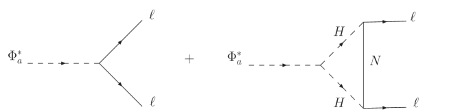
Figure 3: Tree-level and one-loop diagrams contributing to the $CP$ asymmetry in the scalar triplet decay.

Assuming $M_{\Phi_{a}}\ll M_{N}$, the resulting asymmetry is approximately given by Hambye:2003ka

$$\varepsilon\simeq\frac{1}{8\pi^{2}}\,\frac{M_{\Phi_{a}}^{3}}{v^{4}}\,\frac{\mathrm{Im}\,[\mathrm{Tr}\,M_{\nu}^{II}M_{\nu}^{I^{\dagger}}]}{\Gamma_{\Phi}}\,.$$ (20)

Using the relation

$$16\pi v^{2}\Gamma_{\Phi}\sqrt{\mathcal{B}_{\ell}\,\mathcal{B}_{H}}=M_{\Phi_{a}}^{2}\sqrt{\mathrm{Tr}\,M_{\nu}^{II^{\dagger}}M_{\nu}^{II}}\,,$$ (21)

and recalling that the effective seesaw neutrino mass matrix is $\mathcal{M}_{\nu}=M_{\nu}^{I}+M_{\nu}^{II}$, Eq. (20) can be recast in the form Hambye:2005tk

$$\varepsilon\simeq\frac{M_{\Phi_{a}}\sqrt{\mathcal{B}_{\ell}\,\mathcal{B}_{H}}}{4\pi v^{2}}\,\,\frac{\mathrm{Im}\,[\mathrm{Tr}\,M_{\nu}^{II}\mathcal{M}_{\nu}^{\dagger}]}{\sqrt{\mathrm{Tr}\,M_{\nu}^{II^{\dagger}}M_{\nu}^{II}}}\,.$$ (22)

In order to discuss the bounds implied by leptogenesis, it is convenient to write the $CP$ asymmetry $\varepsilon$ as the product

$$\varepsilon=\varepsilon_{\rm max}\sin\delta_{L}\,,$$ (23)

where $\varepsilon_{\rm max}$ is the maximal $CP$ asymmetry and $\delta_{L}$ is an effective leptogenesis phase. Using Eq. (22), it is then straightforward to show that the following upper bound holds

$$\varepsilon_{\rm max}=\frac{M_{\Phi_{a}}}{4\pi v^{2}}\,\left(\mathcal{B}_{\ell}\,\mathcal{B}_{H}\sum m_{\nu_{i}}^{2}\right)^{1/2}\,,$$ (24)

where $m_{\nu_{i}}$ are the light neutrino masses. Clearly, the absolute maximum of the above expression is attained when $\mathcal{B}_{\ell}=\mathcal{B}_{H}=1/2$. This situation, however, does not necessarily corresponds to a maximal baryon asymmetry, since the efficiency of leptogenesis, dictated by the solution of the relevant Boltzmann equations, is not necessarily maximal in such a case. In fact, a numerical study of these equations shows that the efficiency is minimal for $\mathcal{B}_{\ell}=\mathcal{B}_{H}=1/2$ and maximal when either $\mathcal{B}_{\ell}\ll\mathcal{B}_{H}$ or $\mathcal{B}_{\ell}\gg\mathcal{B}_{H}$ Hambye:2005tk .

Assuming no pre-existing asymmetry, the total baryon asymmetry, obtained after partial lepton-to-baryon conversion through the sphalerons, is given by

$$\eta_{B}\simeq-3\times 10^{-2}\,\varepsilon\,\kappa_{f}\,,$$ (25)

where $\kappa_{f}$ is the efficiency factor, normalized in such a way that $\kappa_{f}$ approaches one in the limit of thermal initial $\Phi_{a}$ abundance and no washout. The expression (25), when combined with Eq. (24) leads to a lower bound on the mass $M_{\Phi_{a}}$. Indeed, using the observed value $\eta_{B}^{\rm min}=5.8\times 10^{10}$ ( cf. Eq. (12)), one finds

$$M_{\Phi_{a}}\gtrsim\frac{1.5\times 10^{8}~{}{\rm GeV}}{\kappa_{f}\sqrt{\mathcal{B}_{\ell}\,\mathcal{B}_{H}}}\,\frac{0.05~{}{\rm eV}}{\sqrt{\sum m_{\nu_{i}}^{2}}}\,.$$ (26)

It is possible to obtain a simple estimate of the efficiency of leptogenesis by comparing the total triplet decay rate with the expansion rate of the universe. We define, as usual, the decay parameter

$$K_{\Phi}\equiv\frac{\Gamma_{\Phi}}{H(T=M_{\Phi_{a}})}\,,\quad H(T)=1.66\,g_{\ast}^{1/2}\frac{T^{2}}{M_{P}}\,,$$ (27)

where $H(T)$ is the Hubble rate, $M_{P}\simeq 1.2\times 10^{19}$ GeV is the Planck mass and $g_{\ast}$ is the effective number of relativistic degrees of freedom ($g_{\ast}=106.75$ in the SM). Using Eq. (21), we can rewrite $K_{\Phi}$ in the form

$$K_{\Phi}=\frac{23}{\sqrt{\mathcal{B}_{\ell}\,\mathcal{B}_{H}}}\frac{\sqrt{\sum m_{\nu_{i}}^{2}}}{0.05~{}{\rm eV}}\,.$$ (28)

For not very large values of $K_{\Phi}\gtrsim 1$, an order-of-magnitude estimate of the efficiency factor is $\kappa_{f}\sim 1/K_{\Phi}$ and Eqs. (26) and (27) imply

$$M_{\Phi_{a}}\gtrsim\frac{3.4\times 10^{9}~{}{\rm GeV}}{\mathcal{B}_{\ell}\,\mathcal{B}_{H}}\,,$$ (29)

which for $\mathcal{B}_{\ell}=\mathcal{B}_{H}=1/2$ yields $M_{\Phi_{a}}\gtrsim 1.4\times 10^{10}$ GeV. Clearly, a more precise analysis requires the solution of the full set of Boltzmann equations Hambye:2005tk . Nevertheless, for $\kappa_{f}\simeq 10^{-2}-10^{-3}$ and $\mathcal{B}_{\ell}\sim\mathcal{B}_{H}$, Eq. (26) implies

$$M_{\Phi_{a}}\gtrsim 3\times 10^{10-11}~{}{\rm GeV}\left(\frac{0.05~{}{\rm eV}}{\sqrt{\sum m_{\nu_{i}}^{2}}}\right)\,.$$ (30)

For hierarchical light neutrinos, one has $\sqrt{\sum m_{\nu_{i}}^{2}}\simeq m_{atm}$ and the above bound leads to $M_{\Phi_{a}}\gtrsim 3\times 10^{10-11}~{}{\rm GeV}$. On the other hand, if neutrinos are quasi-degenerate in mass, then the WMAP constraint $\sum m_{\nu_{i}}<0.69$ eV leads to the less restrictive lower limit $M_{\Phi_{a}}\gtrsim 4\times 10^{9-10}~{}{\rm GeV}$. We also note that this bound could be further reduced by about a factor of two, if the dark energy component of the universe is not in the form of a cosmological constant. In the latter case, assuming a dark energy equation of state $p=-w\rho$ with $w<-1$, the present cosmological bound on neutrino masses relaxes to $\sum m_{\nu_{i}}<1.48$ eV Hannestad:2005gj .

Combining the above leptogenesis bounds with the ones shown in Fig. 2, we conclude that the natural implementation of the type-II seesaw mechanism and successful leptogenesis exclude the region of the parameter space where the mass of the triplet $M_{\Phi_{a}}$ is below $10^{9}-10^{10}$ GeV. This in turn implies that the leptoquark $\Phi_{b}$ must be light enough ($M_{\Phi_{b}}\lesssim 10^{6-7}$ GeV) to satisfy the cosmological constraints, thus opening the possibility to test our minimal non-supersymmetric $SU(5)$ GUT scenario at the next generation of collider experiments through the production of light leptoquarks, and particularly, at LHC.

VI Summary

We have investigated in detail the constraints coming from unification of gauge interactions in the minimal extension of the Georgi-Glashow model, where the Higgs sector is composed by $\bm{5}_{H}$, $\bm{15}_{H}$ and $\bm{24}_{H}$. We have shown that the scalar leptoquark $\Phi_{b}$ has to be light in order to achieve unification in agreement with all experimental constraints. Using the constraints coming from triplet seesaw leptogenesis, the upper bound on the leptoquark mass is $M_{\Phi_{b}}\lesssim 10^{6-7}$ GeV. Therefore there is a hope that our scenario could be tested at the next generation of collider experiments through the production of these light leptoquarks.

We have also predicted an upper bound on the total proton decay lifetime which is $\tau_{p}\leq\ 1.4\times 10^{36}$ years. Since at the next generation of proton decay experiments the bounds are expected to be improved by a few orders of magnitude, this minimal non-supersymmetric $SU(5)$ model will be certainly tested or ruled out.

The upper bound on the proton decay lifetime and the exciting possibility to verify the model at future collider experiments make our GUT scenario an appealing candidate for the testability of the idea of grand unification.

Appendix A Two-loop gauge coupling running

The relevant two-loop equations for the running of the gauge couplings take the form

$$\mu\frac{\textrm{d}\,\alpha_{i}(\mu)}{\textrm{d}\,\mu}=\frac{b_{i}}{2\pi}\,\alpha^{2}_{i}(\mu)+\frac{1}{8\pi^{2}}\sum_{j=1}^{3}b_{ij}\,\alpha^{2}_{i}(\mu)\,\alpha_{j}(\mu)+\frac{1}{32\pi^{3}}\,\alpha^{2}_{i}(\mu)\sum_{l=U,D,E}\text{Tr}\,[C_{il}Y^{\dagger}_{l}Y_{l}]\,.$$ (31)

The general formula for $b_{i}$ and $b_{ij}$ coefficients is given in Jones:1981we . Besides the well-known SM coefficients we have:

$$b_{i}^{\Sigma_{8}(\Sigma_{3})}=\left(\begin{array}[]{c}0\\ 0\,(\frac{1}{3})\\ \frac{1}{2}\,(0)\\ \end{array}\right),\qquad b_{i}^{\Phi_{b}}=\left(\begin{array}[]{c}\frac{1}{30}\\ \frac{1}{2}\\ \frac{1}{3}\\ \end{array}\right),\qquad b_{i}^{\Phi_{a}}=\left(\begin{array}[]{c}\frac{3}{5}\\ \frac{2}{3}\\ 0\\ \end{array}\right),$$

$$b_{ij}^{\Sigma_{8}(\Sigma_{3})}=\left(\begin{array}[]{ccc}0&0&0\\ 0&\quad 0\,(\frac{28}{3})&0\\ 0&0&21\,(0)\\ \end{array}\right),\quad b_{ij}^{\Phi_{b}}=\left(\begin{array}[]{ccc}\frac{1}{150}&\frac{3}{10}&\frac{8}{15}\\ \frac{1}{10}&\frac{13}{2}&8\\ \frac{1}{15}&3&\frac{22}{3}\\ \end{array}\right),\quad b_{ij}^{\Phi_{a}}=\left(\begin{array}[]{ccc}\frac{108}{25}&\frac{72}{5}&0\\ \frac{24}{5}&\frac{56}{3}&0\\ 0&0&0\\ \end{array}\right),$$

which we incorporate at the appropriate scales. The $C_{il}$ coefficients are Arason:1991ic :

$$C_{il}=\left(\begin{array}[]{ccc}\frac{17}{10}&\frac{1}{2}&\frac{3}{2}\\ \frac{3}{2}&\frac{3}{2}&\frac{1}{2}\\ 2&2&0\\ \end{array}\right).$$

To insure the proper inclusion of boundary conditions Hall:1980kf at $M_{GUT}$ we set $\left.\alpha^{-1}_{i}\right|_{GUT}=\alpha^{-1}_{GUT}-\lambda_{i}/(12\pi)$, where $\{\lambda_{1},\lambda_{2},\lambda_{3}\}=\{5,3,2\}$. The one-loop equations for the Yukawa couplings can be found, for example, in Ref. Arason:1991ic .

References

- (1) H. Georgi, in Particles and Fields, ed. C. E. Carlson (AIP, New York, 1975) 575.
- (2) H. Fritzsch and P. Minkowski, “Unified Interactions Of Leptons And Hadrons,” Annals Phys. 93 (1975) 193.
- (3) H. Georgi and S. L. Glashow, “Unity Of All Elementary Particle Forces,” Phys. Rev. Lett. 32 (1974) 438.
-
(4)
P. Minkowski,
“Mu E Gamma At A Rate Of One Out Of 1-Billion Muon Decays?,”
Phys. Lett. B 67 (1977) 421 ;
T. Yanagida, in Proceedings of the Workshop on the Unified Theory and the Baryon Number in the Universe, eds. O. Sawada et al., (KEK Report 79-18, Tsukuba, 1979), p. 95;
M. Gell-Mann, P. Ramond and R. Slansky, in Supergravity, eds. P. van Nieuwenhuizen et al., (North-Holland, 1979), p. 315;
S.L. Glashow, in Quarks and Leptons, Cargèse, eds. M. Lévy et al., (Plenum, 1980), p. 707;
R. N. Mohapatra and G. Senjanović, “Neutrino Mass And Spontaneous Parity Nonconservation,” Phys. Rev. Lett. 44 (1980) 912. - (5) K. S. Babu, J. C. Pati and F. Wilczek, “Fermion masses, neutrino oscillations, and proton decay in the light of SuperKamiokande,” Nucl. Phys. B 566 (2000) 33 [arXiv:hep-ph/9812538].
- (6) C. S. Aulakh, B. Bajc, A. Melfo, G. Senjanovic and F. Vissani, “The minimal supersymmetric grand unified theory,” Phys. Lett. B 588 (2004) 196 [arXiv:hep-ph/0306242].
- (7) K. S. Babu, I. Gogoladze, P. Nath and R. M. Syed, “A unified framework for symmetry breaking in SO(10),” Phys. Rev. D 72 (2005) 095011 [arXiv:hep-ph/0506312].
- (8) I. Dorsner and P. Fileviez Pérez, “Unification without supersymmetry: Neutrino mass, proton decay and light leptoquarks,” Nucl. Phys. B 723 (2005) 53 [arXiv:hep-ph/0504276].
- (9) J. R. Ellis and M. K. Gaillard, “Fermion Masses And Higgs Representations In SU(5),” Phys. Lett. B 88 (1979) 315.
- (10) H. Georgi and C. Jarlskog, “A New Lepton - Quark Mass Relation In A Unified Theory,” Phys. Lett. B 86 (1979) 297.
-
(11)
G. Lazarides, Q. Shafi and C. Wetterich,
“Proton Lifetime And Fermion Masses In An SO(10) Model,”
Nucl. Phys. B 181 (1981) 287;
R. N. Mohapatra and G. Senjanović, “Neutrino Masses And Mixings In Gauge Models With Spontaneous Parity Violation,” Phys. Rev. D 23 (1981) 165. - (12) Z. Berezhiani, “2/3 splitting in SUSY GUT: Higgs as Goldstone boson,” arXiv:hep-ph/9703426.
- (13) A. Giveon, L. J. Hall and U. Sarid, “SU(5) unification revisited,” Phys. Lett. B 271 (1991) 138.
- (14) S. Eidelman et al. [Particle Data Group], “Review of particle physics,” Phys. Lett. B 592 (2004) 1.
-
(15)
S. M. Wang [CDF Collaboration],
“Search for Higgs, leptoquarks, and exotics at Tevatron,”
arXiv:hep-ex/0405075;
P. Abreu et al. [DELPHI Collaboration], “Search for leptoquarks and FCNC in e+ e- annihilations at s**(1/2) 183-GeV,” Phys. Lett. B 446 (1999) 62 [arXiv:hep-ex/9903072];
M. Acciarri et al. [L3 Collaboration], “Search for manifestations of new physics in fermion pair production at LEP,” Phys. Lett. B 489 (2000) 81 [arXiv:hep-ex/0005028];
G. Abbiendi et al. [OPAL Collaboration], “Search for leptoquarks in electron photon scattering at s(ee)**(1/2) 209-GeV at LEP,” Phys. Lett. B 526 (2002) 233 [arXiv:hep-ex/0112024];
G. Abbiendi et al. [OPAL Collaboration], “Search for pair-produced leptoquarks in e+ e- interactions at s**(1/2) 189-GeV to 209-GeV,” Eur. Phys. J. C 31 (2003) 281 [arXiv:hep-ex/0305053];
S. Chekanov et al. [ZEUS Collaboration], “A search for resonance decays to lepton + jet at HERA and limits on leptoquarks,” Phys. Rev. D 68 (2003) 052004 [arXiv:hep-ex/0304008].
V. A. Mitsou, N. C. Benekos, I. Panagoulias and T. D. Papadopoulou, “Prospects for scalar leptoquark discovery at the LHC,” arXiv:hep-ph/0411189.
S. Abdullin and F. Charles, “Study of leptoquark pair production at the LHC with the CMS detector,” Phys. Lett. B 464 (1999) 223 [arXiv:hep-ph/9905396].
H. K. Gerberich, “Searches for BSM (non-SUSY) physics at the Tevatron,” arXiv:hep-ex/0511011. - (16) S. M. Barr and I. Dorsner, “A prediction from the type III see-saw mechanism,” arXiv:hep-ph/0507067.
- (17) A. J. Buras, J. R. Ellis, M. K. Gaillard and D. V. Nanopoulos, “Aspects Of The Grand Unification Of Strong, Weak And Electromagnetic Interactions,” Nucl. Phys. B 135 (1978) 66.
- (18) A. H. Guth and E. J. Weinberg, “Cosmological Consequences Of A First Order Phase Transition In The SU(5) Grand Unified Model,” Phys. Rev. D 23 (1981) 876.
- (19) X. y. Li and E. Ma, “Tree-level nondecoupling and the supersymmetric Higgs sector,” J. Phys. G 23 (1997) 885 [arXiv:hep-ph/9608398].
- (20) I. Dorsner and P. Fileviez Pérez, “How long could we live?,” Phys. Lett. B 625 (2005) 88 [arXiv:hep-ph/0410198].
- (21) K. Kobayashi et al. [Super-Kamiokande Collaboration], “Search for nucleon decay via modes favored by supersymmetric grand unification models in Super-Kamiokande-I,” arXiv:hep-ex/0502026.
- (22) P. Fileviez Pérez, “Fermion mixings vs d = 6 proton decay,” Phys. Lett. B 595 (2004) 476 [arXiv:hep-ph/0403286].
- (23) Y. Aoki [RBC Collaboration], “Nucleon decay matrix elements with N(f) = 0 and 2 domain-wall quarks,” Nucl. Phys. Proc. Suppl. 140 (2005) 405 [arXiv:hep-lat/0409114].
- (24) K. Nakamura, “Hyper-Kamiokande: A next generation water Cherenkov detector,” Int. J. Mod. Phys. A 18 (2003) 4053.
- (25) D. N. Spergel et al. [WMAP Collaboration], “First Year Wilkinson Microwave Anisotropy Probe (WMAP) Observations: Determination of Cosmological Parameters,” Astrophys. J. Suppl. 148 (2003) 175.
- (26) M. Fukugita and T. Yanagida, “Baryogenesis Without Grand Unification,” Phys. Lett. B 174 (1986) 45.
- (27) V. A. Kuzmin, V. A. Rubakov and M. E. Shaposhnikov, “On The Anomalous Electroweak Baryon Number Nonconservation In The Early Universe,” Phys. Lett. B 155 (1985) 36.
- (28) T. Hambye and G. Senjanovic, “Consequences of triplet seesaw for leptogenesis,” Phys. Lett. B 582 (2004) 73 [arXiv:hep-ph/0307237].
- (29) T. Hambye, M. Raidal and A. Strumia, “Efficiency and maximal CP-asymmetry of scalar triplet leptogenesis,” arXiv:hep-ph/0510008.
- (30) S. Hannestad, “Neutrino masses and the dark energy equation of state: Relaxing the cosmological neutrino mass bound,” arXiv:astro-ph/0505551.
- (31) D. R. T. Jones, “The Two Loop Beta Function For A G(1) X G(2) Gauge Theory,” Phys. Rev. D 25 (1982) 581.
- (32) H. Arason, D. J. Castano, B. Keszthelyi, S. Mikaelian, E. J. Piard, P. Ramond and B. D. Wright, “Renormalization group study of the standard model and its extensions. 1. The Standard model,” Phys. Rev. D 46 (1992) 3945.
- (33) L. J. Hall, “Grand Unification Of Effective Gauge Theories,” Nucl. Phys. B 178 (1981) 75.