$\bar{B}\to X_{s}l^{+}l^{-}$ IN THE STANDARD MODEL
AND IN TWO-HIGGS-DOUBLET MODELS

We present recent results of the rare semileptonic decay $\bar{B}\to X_{s}l^{+}l^{-}$. We particularly focus on higher order electroweak corrections in the Standard Model (SM) as well as ${\cal O}(\alpha_{s})$ corrections in Two-Higgs-doublet models (THDM), both of which are computed within an effective field theory approach. The calculation of higher order electroweak corrections reveals the presence of enhanced electromagnetic logarithms $\ln(m_{b}^{2}/m_{\ell}^{2})$ in the differential branching ratio. The inclusion of ${\cal O}(\alpha_{s})$ in the THDM reduces the scale dependence of the corresponding Wilson coefficients significantly.

1 Introduction

The inclusive decay $\bar{B}\to X_{s}l^{+}l^{-}$ with $l=e$ or $\mu$ probes the Standard Model directly at the one loop level and is therefore sensitive to new physics. Its branching ratio has been recently measured by both Belle $\!{}^{{\bf?}}$ and BaBar $\!{}^{{\bf?}}$. The experimental results for the differential branching ratio, $\mbox{d}{\cal B}(\bar{B}\to X_{s}l^{+}l^{-})\,/\,\mbox{d}q^{2}$, integrated over the low dilepton invariant mass region, $1\;{\rm GeV}^{2}<m_{\ell\ell}^{2}\equiv q^{2}<6\;{\rm GeV}^{2}$, read

$${\cal B}(\bar{B}\to X_{s}l^{+}l^{-}) = (1.493\pm 0.504^{+0.411}_{-0.321})\times 10^{-6}\;\;\;({\rm Belle})\;,$$ (1)

$${\cal B}(\bar{B}\to X_{s}l^{+}l^{-}) = (1.8\pm 0.7\pm 0.5)\times 10^{-6}\;\;\;({\rm BaBar})\;,$$ (2)

leading to a world average

$${\cal B}(\bar{B}\to X_{s}l^{+}l^{-}) = (1.60\pm 0.51)\times 10^{-6}\;.$$ (3)

Other appealing features of the decay $\bar{B}\to X_{s}l^{+}l^{-}$ are on the one hand the possibility to obtain complementary information compared to the less rare decay $\bar{B}\to X_{s}\gamma$, on the other hand, precision data on both the experimental and theoretical side can be achieved. Indeed, the experimental errors in the branching ratio are expected to be substantially reduced in the near future. On the theoretical side, the predictions are quite well under control because the inclusive hadronic $\bar{B}\to X_{s}\ell^{+}\ell^{-}$ decay rate for low dilepton mass is well approximated by the perturbatively calculable partonic $b\to X_{s}^{\rm parton}\ell^{+}\ell^{-}$ decay rate. Thanks to the recent (practically) complete calculation $\!{}^{{\bf?},{\bf?},{\bf?},{\bf?},{\bf?},{\bf?},{\bf?}}$ of the Next-to-Next-to-Leading Order (NNLO) QCD corrections, the perturbative uncertainties are now below 10%.

However, at the leading order in QED, the branching ratio is proportional to $\alpha_{\mathrm{e}m}^{2}(\mu)$, giving rise to a $\pm 4$% scale uncertainty when the renormalization scale of $\alpha_{\rm em}$ is changed from $\mu={\cal O}(m_{b})$ to $\mu={\cal O}(M_{W})$. This uncertainty can be removed by calculating higher order electroweak corrections. The authors of Ref. $\!{}^{{\bf?}}$ calculated the QED corrections to the Wilson coefficients. In a recent calculation $\!{}^{{\bf?}}$ we confirmed the results of Ref. $\!{}^{{\bf?}}$ and, in addition, computed corrections to the differential branching ratio that originate from QED matrix elements of four-fermion operators. It turns out that the latter corrections are numerically relevant since they are enhanced by large electromagnetic logarithms $\ln(m_{b}^{2}/m_{\ell}^{2})$, which originate from these parts of the QED bremsstrahlung corrections where the photon is emitted collinearly by one of the outgoing leptons.

In the task for the search for new physics beyond the Standard Model it is not only relevant to obtain precise predictions for the process in question with the Standard Model as the underlying theory, but also to perform precision calculations for extensions of the Standard Model (SM). In many extensions of the SM, there are additional one-loop contributions in which non-SM particles propagate in the loop. If the new particles are not considerably heavier than those of the SM, the new contributions to these decays can be as large as the SM ones. One should try to get information on the parameters in a given extension – here the two-Higgs-doublet models – from all processes which allow both a clean theoretical prediction and an accurate measurement. This means that precision studies similar to those for $B\to X_{s}\gamma$ $\!{}^{{\bf?},{\bf?},{\bf?},{\bf?}}$, where higher order QCD corrections are crucial, should also be done for the process $B\to X_{s}l^{+}l^{-}$. We focus on QCD corrections to the Wilson coefficients $C_{9}$ and $C_{10}$ in two-Higgs-doublet models (THDM), which we have calculated in Ref. $\!{}^{{\bf?}}$ and which prove to decrease the scale dependence of the Wilson coefficients significantly. Diagrams with neutral Higgs-boson exchange are neglected. This omission is justified in the type-II model, if the coupling parameter $(m_{\ell}/M_{W})\tan\beta$ is sufficiently smaller than unity. In this case the operator basis is the same as in the SM. Only the matching calculation for the Wilson coefficients gets changed by adding the contributions where the flavor transition is mediated by the exchange of the physical charged Higgs boson. While these extra pieces are known for the coefficients $C_{7}$, $C_{8}$ and $C_{10}$ to two-loop precision $\!{}^{{\bf?},{\bf?},{\bf?},{\bf?}}$ for quite some time, the corresponding results for $C_{9}$ have been first calculated in Ref. $\!{}^{{\bf?}}$ and were confirmed and first published in Ref. $\!{}^{{\bf?}}$.

2 Theoretical framework

2.1 Effective Theory

To describe decays like $B\to X_{s}l^{+}l^{-}$ we use the framework of an effective low–energy theory $\!{}^{{\bf?},{\bf?},{\bf?}}$ with five quarks, obtained by integrating out the heavy degrees of freedom. In the present case these are the $t$-quark, the $W^{\pm}$ and $Z^{0}$ boson as well as — for the THDM calculations — the charged Higgs bosons $H^{\pm}$, whose masses $M_{H}$ are assumed to be of the same order of magnitude as $M_{W}$. We only take into account operators up to dimension six and set $m_{s}=0$. In these approximations the effective Lagrangian relevant for our application (with $|\Delta B|=|\Delta S|=1$) reads

$${\cal L}_{eff}={\cal L}_{\scriptscriptstyle QCD\times QED}(u,d,s,c,b,e,\mu,\tau)+\frac{4G_{F}}{\sqrt{2}}V^{*}_{ts}V_{tb}\left[\sum_{i=1}^{10}C_{i}(\mu){\cal O}_{i}+\sum_{i=3}^{6}C_{iQ}(\mu){\cal O}_{iQ}+C_{b}(\mu){\cal O}_{b}\right].$$ (4)

The operators ${\cal O}_{i}(\mu)$ in the first sum are needed for both our SM and THDM calculation. They read :

$$\begin{array}[]{llll}{\cal O}_{1}\,=&\!(\bar{s}_{L}\gamma_{\mu}T^{a}c_{L})\,(\bar{c}_{L}\gamma^{\mu}T^{a}b_{L})\,,&\quad{\cal O}_{2}\,=&\!(\bar{s}_{L}\gamma_{\mu}c_{L})\,(\bar{c}_{L}\gamma^{\mu}b_{L})\,,\\[4.31415pt] {\cal O}_{3}\,=&\!(\bar{s}_{L}\gamma_{\mu}b_{L})\sum_{q}(\bar{q}\gamma^{\mu}q)\,,&\quad{\cal O}_{4}\,=&\!(\bar{s}_{L}\gamma_{\mu}T^{a}b_{L})\sum_{q}(\bar{q}\gamma^{\mu}T^{a}q)\,,\\[4.31415pt] {\cal O}_{5}\,=&\!(\bar{s}_{L}\gamma_{\mu}\gamma_{\nu}\gamma_{\rho}b_{L})\sum_{q}(\bar{q}\gamma^{\mu}\gamma^{\nu}\gamma^{\rho}q)\,,&\quad{\cal O}_{6}\,=&\!(\bar{s}_{L}\gamma_{\mu}\gamma_{\nu}\gamma_{\rho}T^{a}b_{L})\sum_{q}(\bar{q}\gamma^{\mu}\gamma^{\nu}\gamma^{\rho}T^{a}q)\,,\\[4.31415pt] {\cal O}_{7}\,=&\!\frac{e}{g_{s}^{2}}m_{b}(\bar{s}_{L}\sigma^{\mu\nu}b_{R})F_{\mu\nu}\,,&\quad{\cal O}_{8}\,=&\!\frac{1}{g_{s}}m_{b}(\bar{s}_{L}\sigma^{\mu\nu}T^{a}b_{R})G_{\mu\nu}^{a}\,,\\[4.30554pt] {\cal O}_{9}\,=&\!\frac{e^{2}}{g_{s}^{2}}(\bar{s}_{L}\gamma_{\mu}b_{L})\sum_{l}(\bar{l}\gamma^{\mu}l)\,,&\quad{\cal O}_{10}\,=&\!\frac{e^{2}}{g_{s}^{2}}(\bar{s}_{L}\gamma_{\mu}b_{L})\sum_{l}(\bar{l}\gamma^{\mu}\gamma_{5}l),\par\end{array}$$ (5)

where $T^{a}$ ($a=1,...,8$) are the $SU(3)$ colour generators, and $g_{s}$ and $e$ are the strong and electromagnetic coupling constants, respectively. $q$ and $l$ appearing in the sums run over the light quarks ($q=u,...,b$) and the charged leptons, respectively.

Once QED corrections in the SM are considered, five more operators need to be taken into account. They can be chosen as

$$\begin{array}[]{rl}{\cal O}_{3Q}=&(\bar{s}_{L}\gamma_{\mu}b_{L})\sum_{q}Q_{q}(\bar{q}\gamma^{\mu}q),\vspace{0.2cm}\\ {\cal O}_{4Q}=&(\bar{s}_{L}\gamma_{\mu}T^{a}b_{L})\sum_{q}Q_{q}(\bar{q}\gamma^{\mu}T^{a}q),\vspace{0.2cm}\\ {\cal O}_{5Q}=&(\bar{s}_{L}\gamma_{\mu_{1}}\gamma_{\mu_{2}}\gamma_{\mu_{3}}b_{L})\sum_{q}Q_{q}(\bar{q}\gamma^{\mu_{1}}\gamma^{\mu_{2}}\gamma^{\mu_{3}}q),\vspace{0.2cm}\\ {\cal O}_{6Q}=&(\bar{s}_{L}\gamma_{\mu_{1}}\gamma_{\mu_{2}}\gamma_{\mu_{3}}T^{a}b_{L})\sum_{q}Q_{q}(\bar{q}\gamma^{\mu_{1}}\gamma^{\mu_{2}}\gamma^{\mu_{3}}T^{a}q),\vspace{0.2cm}\\ {\cal O}_{b}=&\frac{1}{12}\left[(\bar{s}_{L}\gamma_{\mu_{1}}\gamma_{\mu_{2}}\gamma_{\mu_{3}}b_{L})(\bar{b}\gamma^{\mu_{1}}\gamma^{\mu_{2}}\gamma^{\mu_{3}}b)-4(\bar{s}_{L}\gamma_{\mu}b_{L})(\bar{b}\gamma^{\mu}b)\right].\end{array}$$ (11)

where $Q_{q}$ are the electric charges of the corresponding quarks ($\frac{2}{3}$ or $-\frac{1}{3}$).

The Wilson coefficients $C_{i}(\mu)$ are found in the matching procedure by requiring that conveniently chosen Green’s functions or on-shell matrix elements are equal when calculated in the effective theory and in the underlying full theory up to ${\cal O}[($external momenta and light masses$)^{2}/M^{2}]$, where $M$ denotes one of the heavy masses like $M_{W}$ or $M_{H}$. The matching scale $\mu_{W}$ is usually chosen to be at the order of $M$, because at this scale the matrix elements or Green’s functions of the effective operators pick up the same large logarithms as the corresponding quantities in the full theory. Consequently, the Wilson coefficients $C_{i}(\mu_{W})$ only pick up “small” QCD corrections, which can be calculated in fixed order perturbation theory.

2.2 Two-Higgs-doublet models

In the following we consider models with two complex Higgs-doublets $\phi_{1}$ and $\phi_{2}$. After spontaneous symmetry breaking these two doublets give rise to two charged ($H^{\pm}$) and three neutral ($H^{0}$, $h^{0}$, $A^{0}$) Higgs-bosons. When requiring the absence of flavour changing neutral currents at the tree-level, as we do in this paper, one obtains two possibilites, the type-I and the type-II THDM $\!{}^{{\bf?}}$. The part of the Lagrangian relevant for our calculation is the Yukawa interaction between the charged physical Higgs bosons $H^{\pm}$ and the quarks (in its mass eigenstate basis):

$${\cal L_{I}}=\frac{\,g}{\sqrt{2}}\left\{\left(\frac{{m_{d}}_{i}}{M_{W}}\right)X\,{\overline{u}_{L}}_{j}V_{ji}\,{d_{R}}_{i}+\left(\frac{{m_{u}}_{i}}{M_{W}}\right)Y\,{\overline{u}_{R}}_{i}V_{ij}\,{d_{L}}_{j}\right\}H^{+}+{\rm h.c.}\,.$$ (12)

The couplings $X$ and $Y$ are

$$\begin{array}[]{llll}X=-\cot\beta,&Y&=&\cot\beta\qquad\mbox{(type-I)},\\ X=\;\;\tan\beta,&Y&=&\cot\beta\qquad\mbox{(type-II)},\end{array}$$ (14)

where $\tan\beta=v_{2}/v_{1}$, with $v_{1}$ and $v_{2}$ being the vacuum expectation values of the Higgs doublets $\phi_{1}$ and $\phi_{2}$, respectively.

3 Standard Model corrections to the decay $\bar{B}\to X_{s}l^{+}l^{-}$

3.1 Electromagnetic corrections to the differential branching ratio

An important quantity in the studies of the rare decay $\bar{B}\to X_{s}l^{+}l^{-}$ is the differential branching ratio, $\mbox{d}{\cal B}(\bar{B}\to X_{s}l^{+}l^{-})\,/\,\mbox{d}q^{2}$, with respect to the invariant mass of the final state lepton pair. The differential branching ratio as a function of $q^{2}$ has a region of on-shell intermediate $\bar{c}c$-resonances like the $J/\Psi$ or the $\Psi^{\prime}$. This region is therefore not accessible perturbatively and one distinguishes two $q^{2}$-windows below and above the $\bar{c}c$-resonances respectively. The low-$q^{2}$-window is taken to be from $1\;{\rm GeV}^{2}<q^{2}<6\;{\rm GeV}^{2}$, whereas the high-$q^{2}$-window is considered for $q^{2}>14.4\;{\rm GeV}^{2}$. Many properties — advantages and disadvantages — of each window are summarized in Ref. $\!{}^{{\bf?}}$. We shall restrict ourselves to the low-$q^{2}$-window here and write the differential decay width as

$$\frac{d\Gamma(\bar{B}\rightarrow X_{s}\,l^{+}l^{-})}{d\hat{s}} = \frac{G_{F}^{2}m_{b,pole}^{5}|V^{*}_{ts}V_{tb}|^{2}\alpha_{em}^{2}(\mu)(1-\hat{s})^{2}}{768\pi^{5}}$$ (15)

$$\times\Big{\{}\!\!\left(4\!+\!\frac{8}{\hat{s}}\right)\!\big{|}\tilde{C}_{7}^{eff}\big{|}^{2}\!+(1+2\hat{s})\big{(}\big{|}\tilde{C}_{9}^{eff}\big{|}^{2}\!\!+\!\big{|}\tilde{C}_{10}^{eff}\big{|}^{2}\big{)}+12\,\mbox{Re}\big{(}\tilde{C}_{7}^{eff}\tilde{C}_{9}^{*\,eff}\big{)}$$

$$\hskip 20.0pt+\Delta^{brems}(\hat{s})\Big{\}}\equiv\frac{G_{F}^{2}m_{b,pole}^{5}|V^{*}_{ts}V_{tb}|^{2}}{48\pi^{3}}\cdot\Phi_{\ell\ell}\,,$$

where we have introduced the notation $\hat{s}\equiv q^{2}/m_{b}^{2}$. The effective Wilson coefficients $\tilde{C}_{i}^{eff}$ contain all corrections relevant for the calculation up to NNLO in QCD $\!{}^{{\bf?},{\bf?},{\bf?},{\bf?},{\bf?},{\bf?}}$ and up to NLO in QED $\!{}^{{\bf?},{\bf?}}$. The last term contains finite gluon bremsstrahlungs corrections $\!{}^{{\bf?}}$. Furthermore, we have included the non-perturbative ${\cal O}(1/m_{b}^{2})$ corrections $\!{}^{{\bf?},{\bf?}}$ and ${\cal O}(1/m_{c}^{2})$ corrections $\!{}^{{\bf?}}$.

In order to minimize the uncertainty stemming from $m_{b,{\rm pole}}^{5}$ and the CKM angles, we normalize the decay width to the measured semileptonic one. Furthermore, to avoid introduction of spurious uncertainties due to the perturbative $b\to X_{c}e\bar{\nu}$ phase-space factor, we follow the $\bar{B}\to X_{s}\gamma$ analysis of Ref. $\!{}^{{\bf?}}$ where

$$C=\left|\frac{V_{ub}}{V_{cb}}\right|^{2}\frac{\Gamma(\bar{B}\to X_{c}e\bar{\nu})}{\Gamma(\bar{B}\to X_{u}e\bar{\nu})}$$ (16)

was used instead. The factor $C=0.58\pm 0.01$ has been recently determined from a global analysis of the semileptonic data $\!{}^{{\bf?}}$. Our expression for the $\bar{B}\to X_{s}\ell^{+}\ell^{-}$ branching ratio finally reads

$${{\rm d}{\cal B}(\bar{B}\to X_{s}\ell^{+}\ell^{-})\over{\rm d}\hat{s}} = {\cal B}(B\to X_{c}e\bar{\nu})_{\rm exp}\;\left|\frac{V_{ts}^{*}V_{tb}}{V_{cb}}\right|^{2}\;\frac{4}{C}\;\frac{\Phi_{\ell\ell}(\hat{s})}{\Phi_{u}}\;,$$ (17)

where $\Phi_{u}=1+{\cal O}(\alpha_{s},\alpha_{\mathrm{e}m},\Lambda^{2}/m_{b}^{2})$ is defined by

$$\Gamma(B\to X_{u}e\bar{\nu})=\frac{G_{F}^{2}m_{b,{\rm pole}}^{5}}{192\pi^{3}}\left|V_{ub}\right|^{2}\;\Phi_{u}.$$ (18)

As stated earlier, the branching ratio has at leading order in QED a $\pm 4$% scale uncertainty due to the renormalization scale dependence of $\alpha_{\rm em}$. The removal of this uncertainty requires the inclusion of higher order electroweak corrections, namely QED corrections to the Wilson coefficients $\!{}^{{\bf?}}$. These corrections have been known for quite a while and imply that the RGE’s for the couplings are coupled differential equations that have a perturbative expansion in $\alpha_{s}$ and $\alpha_{\rm em}$. In Ref. $\!{}^{{\bf?}}$ the results of Ref. $\!{}^{{\bf?}}$ for all the two-loop anomalous dimension matrices that are relevant for the running of the Wilson coefficients from high scales of order ${\cal O}(\mu_{W})$ down to scales of order ${\cal O}(\mu_{b})$ were confirmed.

In addition, corrections to the differential branching ratio that originate from QED matrix elements of four-fermion operators were computed $\!{}^{{\bf?}}$. The loop corrections are not free of infrared divergences and must therefore be considered together with the corresponding bremsstrahlung. The dilepton invariant mass differential decay width is not an infrared safe object with respect to emission of collinear photons. Hence, QED corrections contain an explicit electromagnetic logarithm $\ln(m_{b}^{2}/m_{\ell}^{2})$, which stems from these parts of the QED bremsstrahlung corrections where the photon is emitted collinearly by either of the final state leptons. These enhanced terms always arise as single electromagnetic logarithms accompanied by an electromagnetic coupling $\alpha_{\rm em}$ and therefore do not get resummed. The log-enhanced parts of the QED matrix elements disappear after integration over the whole phase space available but survive and remain numerically important when we restrict $q^{2}$ to the low dilepton invariant mass region, $1\;{\rm GeV}^{2}<q^{2}<6\;{\rm GeV}^{2}$, that we consider. Their numerical impact on the differential branching ratio integrated over the low-$q^{2}$ window is about +5 % for final state electrons and about +2 % for final state muons. The numerical results for the branching ratio integrated over the low-$q^{2}$ region read

$$\hskip-14.22636pt{\cal B}_{\mu\mu} = (1.59\pm 0.11)\times 10^{-6}\;,$$ (19)

$$\hskip-14.22636pt{\cal B}_{ee} = (1.64\pm 0.11)\times 10^{-6}\;.$$ (20)

However, the large effect for electrons gets reduced in size roughly to that of muons once the experimental resolution for collinear photons is taken into account. Precise numbers and more profound explanations on the advent of the collinear logarithm are given in Ref. $\!{}^{{\bf?}}$.

3.2 The forward backward asymmetry ${\cal A}_{FB}$

Another appealing quantity of the decay $\bar{B}\to X_{s}l^{+}l^{-}$ is the so-called forward backward asymmetry ${\cal A}_{FB}$ defined as

$${\cal A}_{FB}(q^{2})\!\equiv\frac{d{{\rm BR}_{\ell\ell}}/dq^{2}(\cos\theta_{\ell}>0)\,-\,d{{\rm BR}_{\ell\ell}}/dq^{2}(\cos\theta_{\ell}<0)}{d{{\rm BR}_{\ell\ell}}/dq^{2}(\cos\theta_{\ell}>0)\,+\,d{{\rm BR}_{\ell\ell}}/dq^{2}(\cos\theta_{\ell}<0)}\;,$$ (21)

where $\theta_{\ell}$ is the angle between the positively charged final state lepton and the initial state $B$-meson in the restframe of the final state lepton pair. The forward backward asymmetry is also nicely reviewed in Ref. $\!{}^{{\bf?}}$. As it is defined as a difference of two quantities over the corresponding sum, it is almost insensitive to hadronic uncertainties since the latter tend to cancel in the ratio. In the SM, the forward backward asymmetry has a zero at $\!{}^{{\bf?},{\bf?}}$

$$q_{0}^{2}=(3.76\pm 0.22_{\rm theory}\pm 0.24_{m_{b}})\,{\rm GeV}^{2}$$ (22)

which is also subject to receive contributions from large electromagnetic logarithms $\!{}^{{\bf?}}$.

The branching ratio and the forward backward asymmetry of the decay $\bar{B}\to X_{s}l^{+}l^{-}$ are important for yet another reason. Contrary to the branching ratio of the rare decay $\bar{B}\to X_{s}\gamma$, which is at lowest order proportional to $\big{|}\tilde{C}_{7}^{eff}\big{|}^{2}$, both the branching ratio of $\bar{B}\to X_{s}l^{+}l^{-}$ and the forward backward asymmetry are sensitive to the sign of $\tilde{C}_{7}^{eff}$. Changing the sign of $\tilde{C}_{7}^{eff}$ results on the one hand in a shift of the branching ratio. This shift is so large that the value of the branching ratio gets moved out of the experimentally allowed range. Therefore the SM sign of $\tilde{C}_{7}^{eff}$ is favored $\!{}^{{\bf?}}$. On the other hand, a change of the sign of $\tilde{C}_{7}^{eff}$ removes the presence of a zero in the forward backward asymmetry $\!{}^{{\bf?}}$. Hence already a rough measurement of the branching ratio and the shape of the forward backward asymmetry can yield useful information about the sign of $\tilde{C}_{7}^{eff}$. The determination of the sign of $\tilde{C}_{7}^{eff}$ is crucial since it allows to strongly constrain the parameter space of certain SUSY models $\!{}^{{\bf?},{\bf?}}$.

4 QCD corrections to the Wilson coefficients $C_{9}$ and $C_{10}$ in the THDM

For the following it is convenient to expand the Wilson coefficients $C_{i}(\mu_{W})$ as

$$C_{i}(\mu_{W})=C^{(0)}_{i}(\mu_{W})+\frac{\alpha_{s}}{(4\pi)}C^{(1)}_{i}(\mu_{W})+\frac{\alpha_{s}^{2}}{(4\pi)^{2}}C^{(2)}_{i}(\mu_{W})+{\cal O}(g_{s}^{6}).$$ (23)

The analytic formulae for the QCD corrections to the Wilson coefficients $C_{9}$ and $C_{10}$ in the THDM at the matching scale $\mu_{W}$ are given in Ref. $\!{}^{{\bf?}}$. In this section we briefly illustrate the impact of these two-loop corrections on $C_{10,\rm{H}}(\mu)$. We then introduce a rescaled Wilson coefficient (see Eq. (23))

$$\hat{C}_{10,\rm{H}}(\mu_{W})\doteq\frac{1}{Y^{2}}\,\frac{4\pi}{\alpha_{s}(\mu_{W})}C_{10,\rm{H}}(\mu_{W}).$$ (24)

In Fig. 1 we plot the quantities

$$\frac{1}{Y^{2}}C_{10,\rm{H}}^{(1)}(\mu_{W})\quad\mbox{and}\quad\frac{1}{Y^{2}}\left(C_{10,\rm{H}}^{(1)}(\mu_{W})+\frac{\alpha_{s}(\mu_{W})}{4\pi}C_{10,\rm{H}}^{(2)}(\mu_{W})\right),$$ (25)

i.e. two approximations of $\hat{C}_{10,\rm{H}}$ as a function of the charged Higgs boson mass $M_{H}$ for the $\overline{\rm{MS}}$- and for the pole mass scheme of the $t$-quark mass. As input parameters we use $\alpha_{s}(M_{Z})=0.119$, $m_{t}^{\rm{pole}}=178.0~{}{\rm GeV}$, $M_{W}=80.4~{}{\rm GeV}$ and $s^{2}_{W}=0.231$ $\!{}^{{\bf?},{\bf?}}$. The upper frame shows these quantities at the relatively low matching scale $\mu_{W}=M_{W}$. As in this case $m_{t}^{\rm{pole}}$ and $\overline{m}_{t}(\mu_{W})$ are numerically almost identical, the one-loop approximations (dotted and dashed lines) are close to each other. The inclusion of the two-loop corrections, however, considerably lowers the (absolute) size of the coefficient for all values of $M_{H}$ considered. In the lower frame a higher matching scale of $\mu_{W}=300$ GeV is chosen. As in this case $m_{t}^{\rm{pole}}$ and $\overline{m}_{t}(\mu_{W})$ differ considerably, the renormalization scheme dependence of the one-loop results is rather large. When taking into account the two-loop corrections (solid and dash-dotted lines), the scheme dependence is drastically reduced.

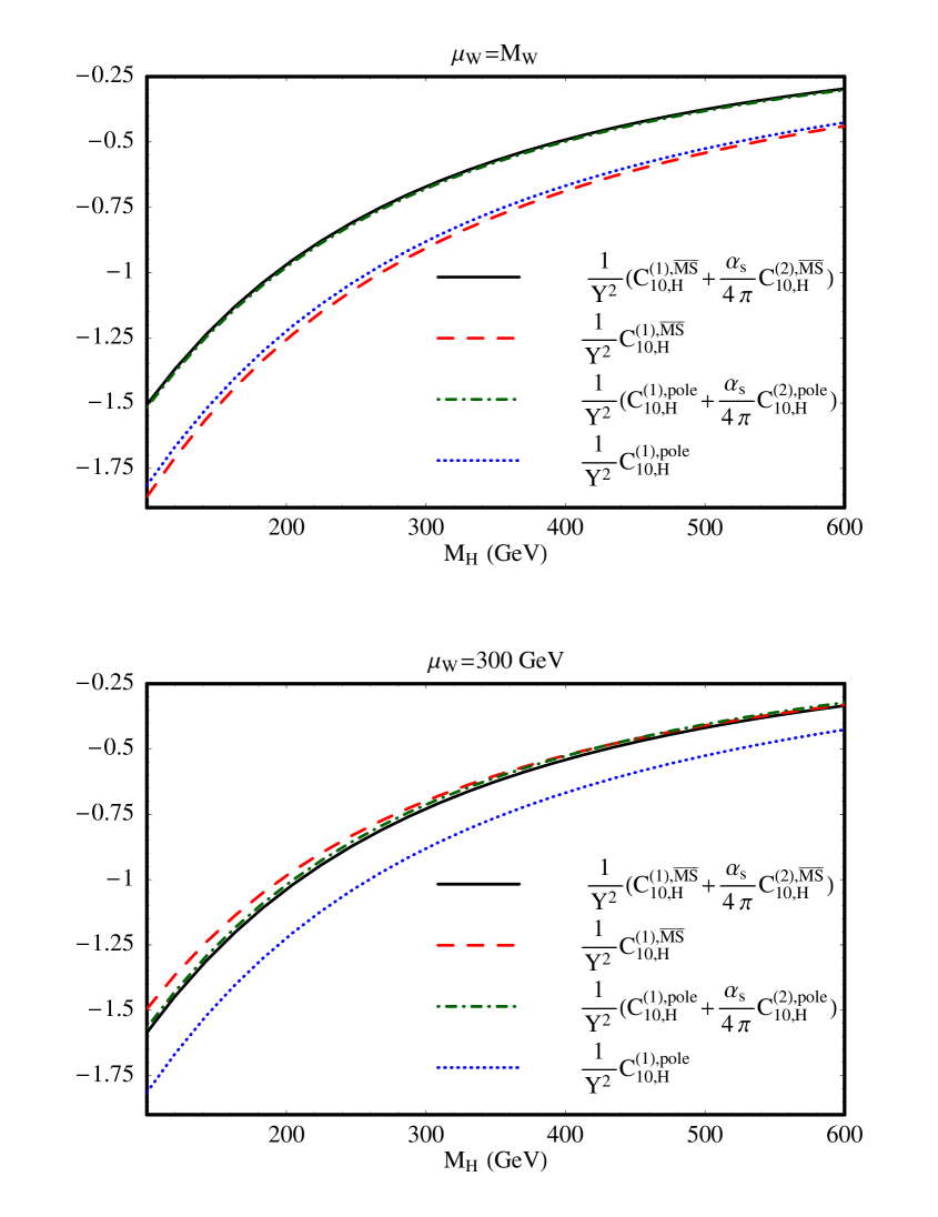
Figure 1: Dependence of the rescaled Wilson coefficient $\hat{C}_{10,\rm{H}}(\mu_{W})$ (see Eq. (24)) on the charged Higgs boson mass $M_{H}$ at the matching scale $\mu_{W}=M_{W}$ (upper frame) and $\mu_{W}=300$ GeV (lower frame). The dashed (dotted) line is the one-loop contribution expressed in $\overline{\rm{MS}}$ -scheme (pole-mass scheme) of the $t$-quark mass, while the solid (dash-dotted) line includes the two-loop corrections in the respective scheme.

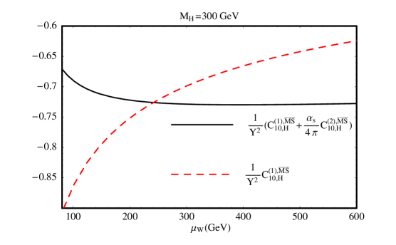
Figure 2: Dependence of the rescaled Wilson coefficient $\hat{C}_{10,\rm{H}}(\mu_{b})$ on the matching scale $\mu_{W}$ (see Eq. (24)) for $M_{H}=300$ GeV. The dashed line shows the one-loop contribution expressed in $\overline{\rm{MS}}$ -scheme for the $t$-quark mass, while the solid line includes the two-loop corrections in the same scheme.

Looking at the renormalization group equation (RGE) $\!{}^{{\bf?}}$ for $\hat{C}_{10,\rm{H}}$, one finds that $\hat{C}_{10,\rm{H}}$ does not run in QCD, i.e.

$$\hat{C}_{10,\rm{H}}(\mu_{b})=\hat{C}_{10,\rm{H}}(\mu_{W})\,,$$ (26)

where the low scale $\mu_{b}$ is of the order of $m_{b}$. In Fig. 2 we show the dependence of $\hat{C}_{10,\rm{H}}(\mu_{b})$ on the matching scale $\mu_{W}$ for $M_{H}=300$ GeV. It can be clearly seen that the inclusion of the two-loop contributions significantly lowers the dependence on $\mu_{W}$. For $\mu_{W}>250$ GeV, $\hat{C}_{10,\rm{H}}(\mu_{b})$ at two-loop precision is nearly $\mu_{W}$-independent. For $\mu_{W}$ between $M_{W}$ and 250 GeV the two-loop Wilson coefficient varies about $\pm 4\%$, whereas the corresponding one-loop coefficient varies about $\pm 11\%$.

5 Summary

The rare decay $\bar{B}\to X_{s}l^{+}l^{-}$ is subject of many contemporary analyses in particle physics since it is a promising channel in the search for new physics beyond the SM. We computed NLO QED corrections to the matrix elements of effective operators and found that these corrections include terms that are enhanced by large electromagnetic logarithms $\ln(m_{b}^{2}/m_{\ell}^{2})$ whose numerical impact on the low-$q^{2}$ branching ratio is in the range of several percent. The zero of the forward backward asymmetry is also expected to get shifted by this type of corrections.

We also showed that the inclusion of QCD corrections to the charged Higgs induced contributions to $C_{10}(\mu_{W})$ in type-I and type-II THDM significantly lowers the dependence of this Wilson coefficient on the scale $\mu_{W}$.

References

References

• [1] M. Iwasaki et al. [Belle Collaboration], [arXiv:hep-ex/0503044].
• [2] B. Aubert et al. [BABAR Collaboration], Phys. Rev. Lett.  93 (2004) 081802 [arXiv:hep-ex/0404006].
• [3] C. Bobeth, M. Misiak and J. Urban, Nucl. Phys. B 574 (2000) 291 [arXiv:hep-ph/9910220].
• [4] H. H. Asatryan, H. M. Asatrian, C. Greub and M. Walker, Phys. Rev. D 65 (2002) 074004 [arXiv:hep-ph/0109140].
• [5] H. H. Asatryan, H. M. Asatrian, C. Greub and M. Walker, Phys. Rev. D 66 (2002) 034009 [arXiv:hep-ph/0204341].
• [6] A. Ghinculov, T. Hurth, G. Isidori and Y. P. Yao, Nucl. Phys. B 685, 351 (2004) [arXiv:hep-ph/0312128].
• [7] P. Gambino, M. Gorbahn and U. Haisch, Nucl. Phys. B673 (2003) 238 [arXiv:hep-ph/0306079].
• [8] M. Gorbahn and U. Haisch, Nucl. Phys. B713 (2005) 291 [arXiv:hep-ph/0411071].
• [9] C. Bobeth, P. Gambino, M. Gorbahn and U. Haisch, JHEP 0404 (2004) 071 [arXiv:hep-ph/0312090].
• [10] T. Huber, E. Lunghi, M. Misiak and D. Wyler, [arXiv:hep-ph/0512066]
• [11] P. Gambino and M. Misiak, “Quark mass effects in anti-B $\to$ X/s gamma,” Nucl. Phys. B 611, 338 (2001) [arXiv:hep-ph/0104034].
• [12] M. Ciuchini, G. Degrassi, P. Gambino and G. F. Giudice, Nucl. Phys. B 527 (1998) 21 [arXiv:hep-ph/9710335].
• [13] F. M. Borzumati and C. Greub, Phys. Rev. D 58 (1998) 074004 [arXiv:hep-ph/9802391];
F. M. Borzumati and C. Greub, Phys. Rev. D 59 (1999) 057501 [arXiv:hep-ph/9809438].
• [14] P. Ciafaloni, A. Romanino and A. Strumia, Nucl. Phys. B 524 (1998) 361 [arXiv:hep-ph/9710312].
• [15] C. Bobeth, M. Misiak and J. Urban, Nucl. Phys. B 567 (2000) 153 [arXiv:hep-ph/9904413].
• [16] S. Schilling, C. Greub, N. Salzmann and B. Toedtli, Phys. Lett. B 616 (2005) 93 [arXiv:hep-ph/0407323].
• [17] C. Bobeth, A. J. Buras, F. Kruger and J. Urban, Nucl. Phys. B 630 (2002) 87 [arXiv:hep-ph/0112305].
• [18] C. Bobeth, Ph.D. thesis Munich (2003) [http://tumb1.biblio.tu-muenchen.de/publ/diss/ph/2003/bobeth.pdf].
• [19] A. J. Buras and M. Münz, Phys. Rev. D 52 (1995) 186 [arXiv:hep-ph/9501281].
• [20] G. Buchalla, A. J. Buras and M. E. Lautenbacher, Rev. Mod. Phys.  68, 1125 (1996) [arXiv:hep-ph/9512380].
• [21] A. J. Buras, [arXiv:hep-ph/9806471].
• [22] S. L. Glashow and S. Weinberg, Phys. Rev. D 15 (1977) 1958.
• [23] U. Haisch, [arXiv:hep-ph/0405122].
• [24] G. Buchalla and G. Isidori, Nucl. Phys. B 525, 333 (1998) [arXiv:hep-ph/9801456].
• [25] G. Buchalla, G. Isidori and S. J. Rey, Nucl. Phys. B 511 (1998) 594 [arXiv:hep-ph/9705253].
• [26] C. W. Bauer, Z. Ligeti, M. Luke, A. V. Manohar and M. Trott, Phys. Rev. D 70 (2004) 094017 [arXiv:hep-ph/0408002].
• [27] T. Huber et. al., work in preparation
• [28] P. Gambino, U. Haisch and M. Misiak, Phys. Rev. Lett.  94 (2005) 061803 [arXiv:hep-ph/0410155].
• [29] A. Ali, E. Lunghi, C. Greub and G. Hiller, Phys. Rev. D 66 (2002) 034002 [arXiv:hep-ph/0112300].
• [30] P. L. Cho, M. Misiak and D. Wyler, Phys. Rev. D 54 (1996) 3329 [arXiv:hep-ph/9601360].
• [31] K. Hagiwara et al. [Particle Data Group Collaboration], Phys. Rev. D 66 (2002) 010001.
• [32] V. M. Abazov et al. [D0 Collaboration], Nature 429 (2004) 638 [arXiv:hep-ex/0406031].