1 Correlations in P-space

Traditionally, particles emitted by high-energy hadronic or heavy ion collisions have been visualised in terms of a collection of points populating what we call primary space $\mathbb{P}$ or P-space, with each particle $i$ represented by a $d$-dimensional vector $\mathbf{x}_{i}=(x_{i1},x_{i2},\ldots,x_{id})$. Examples of P-spaces are three-momentum, with $\mathbf{x}_{i}=(p_{ix},p_{iy},p_{iz})$ and rapidity-azimuth, with $\mathbf{x}_{i}=(y_{i},\phi_{i})$. Particle correlations can be studied either by binning $\mathbb{P}$ with a suitable partition (“coarse-graining”), or by analysing distributions of relative distances between primary vectors $\mathbf{x}_{i}$ directly. In this contribution, we focus exclusively on the latter approach.

Correlations are a matter of definition; typically they are deviations of joint $q$-particle distributions from a pre-defined null hypothesis or reference process[1] such as a uniform distribution or a $q$-fold convolution of the differential one-particle distribution. Under a “dilute-fluid” assumption that correlation strength decreases with particle cluster ($q$-tuple) size, low-order $q$-tuples — particle pairs, triplets, quartets etc. — are usually studied as a first approximation, with higher-order $q$-tuples as perturbations. In general, one selects out of $N$ particles all possible combinations of $q$-tuples ($q=1,2,3,\ldots$) for statistical analysis, using for example cumulants[2] as differential correlation measures. The characterisation of $q$-tuples is therefore fundamental to correlation analysis.

The simplest properties of a given $q$-tuple are its location and size. Location can be defined, for example, as the centre of mass of the $q$ particles,

$$\overline{\mathbf{x}}=\frac{1}{q}\sum_{i=1}^{q}\mathbf{x}_{i}\,,$$ (1)

or as the location of any one of the particles.

In its simplest incarnation, the mathematical realisation of size should be a nonnegative real number which reduces to zero whenever all $q$ particles occupy the same position in $\mathbb{P}$: in other words, size should be a norm based on relative coordinates. Contrary to naive expectation, the best prescription for this is not immediately obvious. While a 2-tuple’s size is clearly described in terms of the distance $|\mathbf{x}_{i}-\mathbf{x}_{j}|$, $q$-tuples of higher order permit a range of choices. In Ref.[3] this problem was addressed in terms of different “topologies”, summarised pictorially in Fig. 1 for some representative 4-tuples.

Figure 1: An event, shown as a collection of $N$ points in the P-space $(y,\phi)$. Also shown are examples of three topologies used to quantify $4$-tuple size.

For every topology, interpair distances can be combined in several ways to form different size estimators. The $q(q-1)/2$ interpair distances making up the GHP topology can, for example, be summed to yield the GHP sum size; or size can be based on the largest of these distances, resulting in the GHP max size estimate. Particle number within $d$-dimensional spheres centered on individual particles defines the Star max size, while the Snake Integral seeks to quantify size in terms of a linear succession of distances between ordered points.

Historically, the GHP max and Star max prescriptions were heuristic inventions within the correlation integral literature: the $q{=}2$ simplest case[4] was extended in Refs.[5] and[6] to the GHP max prescription,

$$C_{q}^{{\rm(GHP)}}(\ell)\equiv\frac{1}{N^{q}}\,\{\mbox{No.\ q-tuples\ }(i_{1},\cdots,i_{q})\mbox{\ with all\ }|\mathbf{x}_{i_{n}}-\mathbf{x}_{i_{m}}|<\ell\}\,,$$ (2)

and in Refs.[7, 8, 9] to the Star max,

$$C_{q}^{{\rm(StarM)}}(\ell)\equiv\frac{1}{N^{q}}\sum_{i=1}^{N}\left(\sum_{j=1}^{N}\theta(\ell-|\mathbf{x}_{i}-\mathbf{x}_{j}|\,)\right)^{q-1}\,,$$ (3)

(with $\theta(x)$ the Heaviside function), which can, on multiplying out the $(q{-}1)$ inner sums and using $\prod_{j}\theta(\ell-|\mathbf{x}_{i}-\mathbf{x}_{j}|\,)=\theta(\ell-\max_{j}(|\mathbf{x}_{i}-\mathbf{x}_{j}|\,))$, be made to exhibit the Star max prescription on the $q$-tuple $(i,j_{1},\cdots,j_{q-1})$ explicitly,

$$C_{q}^{{\rm(StarM)}}(\ell)=\frac{1}{N^{q}}\sum_{i=1}^{N}\;\;\sum_{j_{1},\cdots,j_{q-1}=1}^{N}\theta(\ell-\max_{k}\{\,|\mathbf{x}_{i}-\mathbf{x}_{j_{k}}|\,\}\,)\,.$$ (4)

Factorial extensions were published in Ref.[3]. Note that, in summing indiscriminately over all $q$-tuples, the above correlation integrals implicitly assume that correlation structure is independent of location.

2 Q-space by example

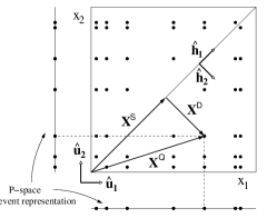
The concept of Q-spaces is not new: In high-energy hadronic collisions, two-particle correlations have long been visualised in two-particle spaces[10]. Figure 2 illustrates by means of a simple example how a Q-space is constructed from P-space. A typical event in a one-dimensional ($d{=}1$) primary space is represented by the dots on the lines below the $\mathbf{x}_{1}$ axis and to the left of the $\mathbf{x}_{2}$ axis. Particle pairs are then represented by all possible dots in the $Q{=}2$ space as shown by representative dashed lines.

Each pair in this example is represented by a vector $\mathbf{X}^{Q}$ as shown. The location corresponds to the component vector $\mathbf{X}^{S}$ along the diagonal, and the 2-tuple size to the magnitude of $\mathbf{X}^{D}$, since $|\mathbf{X}^{S}|=|x_{1}+x_{2}|/\sqrt{2}=\sqrt{2}\,\overline{\mathbf{x}}$ and $|\mathbf{X}^{D}|=|x_{1}-x_{2}|/\sqrt{2}$. This can be derived algebraically by using the Q-space representation $\mathbf{X}^{Q}=x_{1}\hat{\mathbf{u}}_{1}+x_{2}\hat{\mathbf{u}}_{2}$ in terms of the index unit vectors $\hat{\mathbf{u}}_{1,2}$, which are rotated to the basis vectors $\hat{\mathbf{h}}_{1,2}$ shown in Fig. 2 to find $\mathbf{X}^{S}=\hat{\mathbf{h}}_{1}\,(\hat{\mathbf{h}}_{1}\mathbf{\,\cdot\,}\mathbf{X}^{Q})$ and $\mathbf{X}^{D}=\hat{\mathbf{h}}_{2}\,(\hat{\mathbf{h}}_{2}\mathbf{\,\cdot\,}\mathbf{X}^{Q})$.

Figure 2: Example of Q-space for $q{=}2,d{=}1$. The primary space event, represented on the margins, maps onto particle pairs in the Q-space square. Vector $\mathbf{X}^{Q}$, representing a particular pair, decomposes into a location vector $\mathbf{X}^{S}$ and a size vector $\mathbf{X}^{D}$. Unit vectors $\hat{\mathbf{u}}_{1,2}$ are rotated to $\hat{\mathbf{h}}_{1}$ and $\hat{\mathbf{h}}_{2}$ which span sum space and difference space respectively.

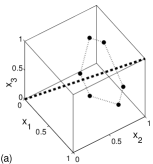
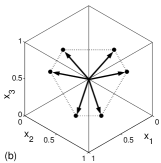
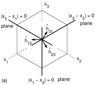
Correspondingly, 3-tuples can be visualised for one-dimensional P-spaces as shown in Fig. 3. Here, one particular ordered triplet is shown in all its exchange-permutation incarnations, all of which represent the same unordered triplet; the associated symmetry is clearly visible when viewing the Q-space down the main diagonal as in Fig. 3(b). The set of unit vectors $(\hat{\mathbf{u}}_{1},\hat{\mathbf{u}}_{2},\hat{\mathbf{u}}_{3})$ is transformed to

$$\hat{\mathbf{h}}_{1} = (\hat{\mathbf{u}}_{1}+\hat{\mathbf{u}}_{2}+\hat{\mathbf{u}}_{3})/\sqrt{3}$$ (5)

$$\hat{\mathbf{h}}_{2} = (\hat{\mathbf{u}}_{1}-\hat{\mathbf{u}}_{2})/\sqrt{2}$$ (6)

$$\hat{\mathbf{h}}_{3} = (\hat{\mathbf{u}}_{1}+\hat{\mathbf{u}}_{2}-2\hat{\mathbf{u}}_{3})/\sqrt{6}$$ (7)

where $\hat{\mathbf{h}}_{1}$ points along the main diagonal (shown as the dashed line), while $\hat{\mathbf{h}}_{2}$ and $\hat{\mathbf{h}}_{3}$ span the plane, indicated by the dotted lines in Fig. 3, which is normal to the main diagonal. This normal plane exemplifies difference space $\mathbb{D}_{3}$, within which only relative coordinates appear, while the main diagonal represents the sum space $\mathbb{S}_{3}$ measuring, once again, $q$-tuple location.

Figure 3: A $3$-tuple (with $d{=}1$) showing (a) a $3$-tuple point plus its five permutation-symmetric counterparts and the main diagonal (dashed line), and (b) the same system when viewed down the main diagonal. Also shown are the corresponding difference vectors $\mathbf{X}^{D}$. The dotted lines are coplanar with the difference space $\mathbb{D}_{3}$.

3 Formalism for Q-space

The general formalism for vectors in $\mathbb{Q}$ is now easily understood. The particle vectors $\mathbf{x}_{i},i=1,\ldots q$ of a $q$-tuple in $d$-dimensional primary space $\mathbb{P}$ are combined into the Q-space-vector

$$\mathbf{X}^{Q}=\sum_{i=1}^{q}\mathbf{x}_{i}\,\hat{\mathbf{u}}_{i}\,.$$ (8)

$\mathbb{Q}$ is spanned by unit vectors which are the product of unit vectors $\hat{\mathbf{u}}_{i},i=1,\ldots,q$ living in index-space $\mathbb{I}_{q}$ and the basis vectors of $\mathbb{P}$ (implicit in $\mathbf{x}_{i}$). The $d$-dimensional sum space $\mathbb{S}_{q}$ is spanned by

$$\hat{\mathbf{h}}_{1}=\frac{1}{\sqrt{q}}\;\sum_{i=1}^{q}\hat{\mathbf{u}}_{i}$$ (9)

and the basis vectors of $\mathbb{P}$. The corresponding index-space projection of $\mathbf{X}^{Q}$ onto sum space, $\mathbf{X}^{S}\equiv\hat{\mathbf{h}}_{1}\,(\hat{\mathbf{h}}_{1}\mathbf{\,\cdot\,}\mathbf{X}^{Q})$, is given by

$$\mathbf{X}^{S}=\frac{1}{\sqrt{q}}\sum_{i=1}^{q}\mathbf{x}_{i}=\sqrt{q}\;\overline{\mathbf{x}}\,,$$ (10)

where $\overline{\mathbf{x}}$ is the $q$-tuple CMS as before. Furthermore, the algebraic complement of $\mathbb{S}_{q}$ is spanned by the set of $(q-1)$ orthonormal vectors in $\mathbb{I}_{q}$

$$\hat{\mathbf{h}}_{2} = (\hat{\mathbf{u}}_{1}-\hat{\mathbf{u}}_{2})/\sqrt{2}\,,$$ (11)

$$\hat{\mathbf{h}}_{3} = (\hat{\mathbf{u}}_{1}+\hat{\mathbf{u}}_{2}-2\hat{\mathbf{u}}_{3})/\sqrt{6}$$ (12)

$$\vdots$$

$$\hat{\mathbf{h}}_{q} = \frac{1}{\sqrt{q(q-1)}}\;\sum_{i=1}^{q-1}(\hat{\mathbf{u}}_{i}-\hat{\mathbf{u}}_{q})\,,$$ (13)

which, together with the $\mathbb{P}$ basis, are used to define a basis for difference space $\mathbb{D}_{q}$. The index space projection of $\mathbf{X}^{Q}$ onto $\mathbb{D}_{q}$ is given by

$$\mathbf{X}^{D}\equiv\sum_{i=2}^{q}\hat{\mathbf{h}}_{i}\left(\hat{\mathbf{h}}_{i}\mathbf{\,\cdot\,}\mathbf{X}^{Q}\right)\,.$$ (14)

Since every $\mathbf{X}^{Q}\in\mathbb{Q}$ has a unique decomposition into $\mathbf{X}^{S}$ and $\mathbf{X}^{D}$, $\mathbb{Q}$ is the direct sum of $\mathbb{S}_{q}$ and $\mathbb{D}_{q}$. The relationship between the different spaces can hence be summarised as

$$\mathbb{I}_{q}\otimes\mathbb{P}=\mathbb{Q}=\mathbb{S}_{q}\oplus\mathbb{D}_{q}\,,$$ (15)

corresponding to the dimensionality relation $\dim(\mathbb{I}_{q})\times\dim(\mathbb{P})=\dim(\mathbb{Q})=\dim(\mathbb{S}_{q})+\dim(\mathbb{D}_{q})$  or, explicitly,  $q\times d=qd=d+(q-1)d$.

Within this framework, the first and most obvious measure of size is the 2-norm of $\mathbf{X}^{D}$. Starting either with Eq. (14) or by subtraction, $\mathbf{X}^{D}=\mathbf{X}^{Q}-\mathbf{X}^{S}$, we find the suggestive form

$$\mathbf{X}^{D}=\sum_{i=1}^{q}\left(\mathbf{x}_{i}-\overline{\mathbf{x}}\right)\hat{\mathbf{u}}_{i},$$ (16)

which yields

$$\left|\mathbf{X}^{D}\right|=\frac{1}{\sqrt{q}}\left[\;\sum_{i<j=1}^{q}\left(\mathbf{x}_{i}-\mathbf{x}_{j}\right)^{2}\right]^{1/2}\,,$$ (17)

which, apart from the prefactor, is exactly the GHP 2-sum or rms size measure. The GHP 2-sum thus appears to be the natural measure of size in Q-space.

4 Generalised $p$-sizes

While the above result represents a strong endorsement of the Q-space approach to multiparticle correlations, there is more. Generalised $p$-norms are the extension of Eq. (17) to arbitrary $p\geq 1$: Given an $m$-dimensional vector $\mathbf{A}=(a_{1},\dots,a_{m})$, the p-norm of $\mathbf{A}$ is defined by

$${|\!|\mathbf{A}|\!|}_{\,p}\equiv\Bigl{[}\;\sum_{i=1}^{m}|a_{i}|^{p}\,\Bigr{]}^{1/p}\,.$$ (18)

Special cases are the $p{=}2$ norm appearing in Eq. (17) and the “max” norm,

$$\lim_{p\to\infty}{|\!|A|\!|}_{\,p}=\max_{i}(\,|a_{i}|\,)\,.$$ (19)

The condition $p\geq 1$, required for ${|\!|\mathbf{A}|\!|}_{\,p}$ to satisfy the Minkowski inequality ${|\!|\mathbf{A}+\mathbf{B}|\!|}_{\,p}\leq{|\!|\mathbf{A}|\!|}_{\,p}+{|\!|\mathbf{B}|\!|}_{\,p}$, can be relaxed to $p\in\mathbb{R}$ if we do not insist on ${|\!|A|\!|}_{\,p}$ being a norm and allow it to be merely a “size measure” or “$p$-size”. We then also have negative-$p$ sizes and in particular

$$\lim_{p\to\;-\infty}{|\!|A|\!|}_{\,p}=\min_{i}(\,|a_{i}|\,)\,,\qquad|a_{i}|\neq 0\ \forall i\,.$$ (20)

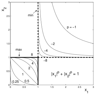
Fig. 4 shows as a simple example for a two-component vector $\mathbf{A}=(x_{1},x_{2})$ the set of isonorms satisfying ${|\!|\mathbf{A}|\!|}_{\,p}=1=\left[\,|x_{1}|^{p}+|x_{2}|^{p}\,\right]^{1/p}$ i.e. a set of curves showing which vectors $\mathbf{A}$ have the same “$p$-size”. Only positive $x_{1}$ and $x_{2}$ are shown as ${|\!|\mathbf{A}|\!|}_{\,p}$ is reflection-symmetric about $x_{1}{=}0$ and $x_{2}{=}0$. The usual circle for constant $2$-norm is complemented by the straight diagonal line (or, in the full plane, diamond shape) of $p{=}1$ and various shapes in between. Of particular interest are the max and min size measures shown as the solid line and dashed line respectively.

Figure 4: Example of $p$-sizes: A vector $\mathbf{A}=(x_{1},x_{2})$ has many different norms or, more generally, $p$-sizes. Conversely, different sets of vectors $\mathbf{A}$ have the same $p$-sizes, as shown in this picture. The usual quarter-circle Pythagorean norm ($p{=}2$) is complemented by various convex and concave “isonorm” curves. Of particular interest are the $p=+\infty$ (maximum) and $p=-\infty$ (minimum) sizes.

Based on the above, we can define a “GHP sum $p$-size” as follows:

$$S_{q,p}^{{\rm(GHP)}}\equiv\Bigl{[}\sum_{i<j=1}^{q}|\mathbf{x}_{i}-\mathbf{x}_{j}|^{p}\Bigr{]}^{1/p}\,,\quad p\neq 0$$ (21)

which for $p\geq 1$ is a norm. Eq. (17) is seen to be the special case $S_{q,2}^{{\rm(GHP)}}=\sqrt{q}\;{|\!|\mathbf{X}^{D}|\!|}_{\,2}$, while the GHP max definition is the special case $p\to\infty$,

$$S_{q,\infty}^{{\rm(GHP)}}=\max_{i<j=1}^{q}|\mathbf{x}_{i}-\mathbf{x}_{j}|\,,$$ (22)

representing the size prescription used in the correlation integral (2).

A given Q-space vector $\mathbf{A}$ will therefore yield a set of size measures $\left\{{|\!|\mathbf{A}|\!|}_{\,p}\;|\;p\in\mathbb{R},\;p\neq 0\right\}$. which includes the “min”, “max” as well as the usual 2-norms. An infinite set of $p$-sizes of a given $q$-tuple is, however, mostly redundant; for practical purposes, a subset such as $p\in\{-\infty,0.5,2,+\infty\}$ is probably sufficient.

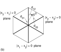
The sizes $S_{q,p}$ can be understood in terms of projections in Q-space as follows. Define the set of pair plane normal vectors $\hat{\mathbf{h}}_{ij}\equiv(\hat{\mathbf{u}}_{i}-\hat{\mathbf{u}}_{j})/\sqrt{2}$; these can be considered to span the respective pair $(i,j)$’s difference space $\mathbb{D}_{2}^{(i,j)}$. Eq. (21) then can be written as

$$S_{q,p}^{{\rm(GHP)}}=\Bigl{[}\sum_{i<j=1}^{q}|\hat{\mathbf{h}}_{ij}\mathbf{\,\cdot\,}\mathbf{X}^{Q}|^{p}\Bigr{]}^{1/p}\,.$$ (23)

The set of $\hat{\mathbf{h}}_{ij}$’s are clearly not mutually orthogonal, given that $q(q-1)/2$ vectors $\hat{\mathbf{h}}_{ij}$ all live in the $(q-1)$-dimensional difference space $\mathbb{D}_{q}$: indeed, we have $\hat{\mathbf{h}}_{ij}\mathbf{\,\cdot\,}\hat{\mathbf{h}}_{kl}=(\delta_{ik}+\delta_{jl}-\delta_{il}-\delta_{jk})/2$ and, conversely, Eqs. (11)–(13) show that the $\hat{\mathbf{h}}_{q\geq 2}$ are simple sums of the $\hat{\mathbf{h}}_{ij}$’s. Fig. 5 shows, for the simple case $q{=}3$ and $d{=}1$, the normal vectors in the difference space $\mathbb{D}_{3}$ (equivalent to viewing the $\mathbb{Q}$ cube of Fig. 3(a) down the main diagonal) as well as the distances from the respective pair planes $d_{ij}=|\mathbf{x}_{i}-\mathbf{x}_{j}|/\sqrt{2}$.

Figure 5: Example ($d{=}1$, $q{=}3$) of the nonorthogonal projection (not decomposition!) of Q-space vectors in terms onto “pair plane normals” $\hat{\mathbf{h}}_{ij}$. The difference space vector $\mathbf{X}^{D}$, shown as a point in (b), is projected onto the pair plane normal vectors $\hat{\mathbf{h}}_{12}$, $\hat{\mathbf{h}}_{23}$ and $\hat{\mathbf{h}}_{31}$ to yield the distances $d_{ij}$ between $\mathbf{X}^{D}$ and the respective pair planes $|\mathbf{x}_{i}-\mathbf{x}_{j}|=0$. The views are once again down the main diagonal.

5 Q-space and other size measures

The symmetry of Q-space clearly favours the GHP topology over the corresponding Star and Snake topologies. It is possible, nevertheless, to accommodate the latter into Q-space. A simple ad hoc definition of the Star $p$-size of the $q$-tuple centered on $\mathbf{x}_{i}$ would be

$$S_{q,p}^{{\rm(Star)}}(\mathbf{x}_{i})\equiv\Bigl{[}\sum_{j=1}^{q}|\mathbf{x}_{i}-\mathbf{x}_{j}|^{p}\Bigr{]}^{1/p}\,,\quad p\neq 0\,.$$ (24)

This is the $p$-generalised size measure corresponding to the Star max correlation integrals of Eq. (3)–(4). Alternatively, we can, for the Star $q$-tuple centered on $i{=}1$, define a vector $\mathbf{X}^{S}_{{\rm Star}}(\mathbf{x}_{1})\equiv\sqrt{q}\,\mathbf{x}_{1}\hat{\mathbf{h}}_{1}$ and from this find the vector

$$\mathbf{X}^{D}_{{\rm Star}}(\mathbf{x}_{1})\equiv\mathbf{X}^{Q}-\mathbf{X}^{S}_{{\rm Star}}(\mathbf{x}_{1})=(\mathbf{x}_{2}-\mathbf{x}_{1})\hat{\mathbf{u}}_{2}+\cdots+(\mathbf{x}_{q}-\mathbf{x}_{1})\hat{\mathbf{u}}_{q}\,;$$ (25)

then the size measure (24) can be applied directly in terms of its $\hat{\mathbf{u}}_{j}$ components. Clearly, the pair $(\mathbf{X}^{S}_{{\rm Star}}(\mathbf{x}_{1}),\mathbf{X}^{D}_{{\rm Star}}(\mathbf{x}_{1}))$ is not orthogonal to $\hat{\mathbf{h}}_{1}$ and hence lives neither in $\mathbb{S}_{q}$ nor $\mathbb{D}_{q}$; also, this pair will be different for every $q$-tuple centre $\mathbf{x}_{i}$. This is consistent with the fact that sizes of Star $q$-tuples are, by definition, different for the different centre particles.

Star and Snake topologies can be accommodated in the Q-space presented here, but, due to their obvious asymmetry, do not fit comfortably into the explicitly symmetric Q-space framework. Other approaches such as conditional spaces (for the Star) and spaces based on strict ordering such as in time series (for the Snake) will probably yield more natural interpretations for these cases.

6 Summary

It is becoming clear that the concept of Q-spaces is yielding insight into the fundamental structure of correlations of point sets. As subspaces of the final-state phase space $q=N$, Q-spaces have a solid theoretical and historical foundation, while offering a structured set of numbers characterising $q$-tuples, starting with location and size. Generalising simple notions of norms to an infinite set of $p$-sizes, we find that the “max” and 2-sum sizes are just special cases within this wider set. Nonorthogonal “pair planes” projections are found to be important, in keeping with the obvious fact that relative distances are also mutually constrained and hence dependent.

Most importantly, the usual 2-norm of the difference space vector is found to be the GHP sum size prescription, which therefore should be afforded more attention in higher order correlation analyses.

Extensions such as shape characterisers and higher-order measures of size are easily conjured up.

References

- [1] H.C. Eggers, in: 30th Int. Symp. on Multiparticle Dynamics, World Scientific (2001) pp. 291–302; hep-ex/0102005
- [2] A. Stuart and J.K. Ord, Kendall’s Advanced Theory of Statistics, Vol.1, fifth edition, Oxford University Press, New York (1987).
- [3] P. Lipa, P. Carruthers, H. C. Eggers and B. Buschbeck, Phys. Lett. B285, 300 (1992); H. C. Eggers, P. Lipa, P. Carruthers and B. Buschbeck, Phys. Rev. D48, 2040 (1993).
- [4] P. Grassberger and I. Procaccia, Phys. Rev. Lett. 50, 346 (1983).
- [5] Hentschel and Procaccia, Physica 8D, 435 (1983).
- [6] P. Grassberger, Phys. Lett. A97, 227 (1983).
- [7] G. Paladin and A. Vulpiani, Lett. Nuovo Cimento 41, 82 (1984).
- [8] K. Pawelzik and H. G. Schuster, Phys. Rev. A35,481 (1987).
- [9] H. Atmanspacher, H. Scheingraber and G. Wiedenmann, Phys. Rev. A40, 3954 (1989).
- [10] L. Foà, Phys. Rep. 22, 1 (1975).