November 2005

We review the recent experimental and theoretical progress in the determination of $|V_{ud}|$ and $|V_{us}|$, and the status of the most stringent test of CKM unitarity. Future prospects on $|V_{cd}|$ and $|V_{cs}|$ are also briefly discussed.

1 Introduction

The most precise constraints on the size of the elements of the CKM matrix [1, 2] are extracted from the low-energy $s\rightarrow u$ and $d\rightarrow u$ semileptonic transitions. Combining the precise determinations of $|V_{ud}|$ and $|V_{us}|$ extracted from these processes we can perform the most stringent test of CKM unitarity, namely we can probe the validity of the relation

$$|V_{ud}|^{2}+|V_{us}|^{2}+|V_{ub}|^{2}=1~{}.$$ (1)

at the 0.1% level. In particular, the best determination of $|V_{us}|$ is obtained from semileptonic $K$ decays ($K_{\ell 3}$ and $K_{\ell 2}$), while the most stringent constraints on $|V_{ud}|$ are obtained from superallowed Fermi transitions (and, to a minor extent, from neutron and pion beta decays). As we will discuss in the following, in the last few years there has been a substantial progress - both from the theoretical and the experimental side - in the determination of these two matrix elements.

In all cases the key observation which allow a precise extraction of the CKM factors is the conservation of the vector current at zero momentum transfer in the $SU(N)$ limit and the non-renormalization theorem. The latter implies that the relevant hadronic form factors are completely determined up to tiny second order isospin-breaking corrections in the $d\rightarrow u$ case [3] or SU(3)-breaking corrections in the $s\rightarrow u$ case [4]. As a result of this fortunate situation, the accuracy on $|V_{us}|$ is approaching the 1% level and the one on $|V_{ud}|$ is already below the 0.05% level.

The present accuracy on $|V_{ud}|$ and $|V_{us}|$ is such that the contribution of $|V_{ub}|^{2}\approx 2\times 10^{-5}$ in the relation (1) can safely be neglected, and the uncertainty of the first two terms is comparable. In other words, to a high degree of accuracy we can set

$$V_{us}=\sin\theta_{c}~{},\qquad V_{ud}=\cos\theta_{c}~{},$$ (2)

as in the original Cabibbo theory [1], and $|V_{us}|$ and $|V_{ud}|$ provide two independent determinations of the Cabibbo angle both around the 1% level.

In the following sections we will review the determinations of $|V_{us}|$ and $|V_{ud}|$ from the main observables mentioned above. We will also briefly analyze alternative strategies to extract $|V_{us}|$ from $\tau$ and hyperon decays, as well as the future prospects on $|V_{cs}|$ and $|V_{cd}|$. The main recent results on $|V_{us}|$ and $|V_{ud}|$ are then summarized and combined in the last section, where we will discuss the accuracy to which Eq. (1) is satisfied and we will provide a final global estimate of the Cabibbo angle.

2 The extraction of $V_{ud}$

The value of $V_{ud}$ has been extracted from 1) super-allowed, $0^{+}\rightarrow 0^{+}$, nuclear beta decays, 2) neutron beta decays, $n\rightarrow pe\nu$, and 3) pion beta decay $\pi^{+}\rightarrow\pi^{0}e^{+}\nu$. The latter two, subsequently discussed in this report, have smaller overall theoretical uncertainties and may in the long term be better ways to obtain $V_{ud}$; but currently, only super-allowed beta decays determine $V_{ud}$ to better than 0.05%.

2.1 Super-allowed Fermi transitions

The so-called super-allowed, $0^{+}\rightarrow 0^{+}$, Fermi transitions between nuclei are very special [5]. Because they proceed (at the tree level) through pure weak vector current interactions, which are conserved in the $m_{d}=m_{u}$ limit; they are not renormalized by strong interactions at $q^{2}=0$. Hence, they are ideally suited for cleanly extracting $V_{ud}$ with high precision. Corrections due to $q^{2}\neq 0$ and $m_{d}\neq m_{u}$ are negligibly small; so, one needs only to control uncertainties in the electroweak radiative corrections, isospin violating electromagnetic effects and nuclear structure dependence. How well that can be done is the subject of this section.

Last year, the prevailing value of $V_{ud}$ obtained by averaging the nine best measured super-allowed $\beta$-decays was [6, 7]

$$V_{ud}=0.9740(1)(3)(4)\rightarrow 0.9740(5)\hskip 28.45274pt{\rm(2004\ value)}$$ (3)

where the errors are experimental, nuclear theory and quantum loop corrections. The very small experimental error illustrates the power of this averaging procedure. The largest uncertainty, associated with weak axial-vector induced loop effects [8] primarily through $\gamma W$ box diagrams, represents model dependent hadronic effects which until recently [9] were thought to be essentially irreducible or at least very difficult to reduce.

Two developments have led to a recent improvement in $V_{ud}$ by nearly a factor of 2. First, new global studies of super-allowed $\beta$-decays by Hardy and Towner [10], and by Savard et al. [11], have provided a more consistent treatment of $Q$ values and lifetimes used in $ft$ determinations, which in turn give $V_{ud}$ via the master formula

$$|V_{ud}|^{2}=\frac{2984.48(5)~{}{\rm s}}{ft(1+RC)}$$ (4)

In that expression, RC designates the total effect of all radiative corrections from quantum loops as well as nuclear structure and isospin violating effects. RC is nucleus dependent, ranging from about +3.1% to +3.6% for the nine best measured super-allowed decays. That difference is of critical importance in bringing the values of $V_{ud}$ obtained from separate decays into agreement with one another. The magnitude of the corrections is essential for establishing unitarity, as we shall see.

A second major advance in the determination of $V_{ud}$ stems from a new study of the quantum loop corrections coming from the problematic $\gamma{\rm W}$ box diagram due to weak axial-vector contributions. Previously, those effects, along with other smaller axial-vector current contributions, were found to shift the RC by about

$$\frac{\alpha}{2\pi}\biggl{[}\ln\frac{m_{Z}}{m_{A}}+A_{g}+2C_{\rm Born}\biggr{]}$$ (5)

where $A_{g}={-0.34}$ is a one-loop QCD correction to the short-distance logarithmic loop contribution and $C_{Born}\simeq 0.8g_{A}(\mu_{p}+\mu_{n})\simeq 0.9$ represents long-distance loop effects. The problematic intermediate loop momentum region was roughly estimated by employing $m_{A}\simeq 1.2{\rm GeV}$ in the log, while the crudely obtained error of $\pm 8\times 10^{-4}$ in that quantity (which leads to $\pm 4\times 10^{-4}$ in $V_{ud}$) was found [6, 8] by allowing the $m_{A}$ cut-off scale to vary up or down by a factor of 2.

A new analysis [9] of the $\gamma{\rm W}$ box diagram now divides the loop momentum into 3 integration regions:

$$(1.5~{}{\rm GeV})^{2}\leq Q^{2}_{I}<\infty$$

$$(0.82~{}{\rm GeV})^{2}\leq Q^{2}_{II}<(1.5~{}{\rm GeV})^{2}$$

$$0\leq Q^{2}_{III}<(0.82~{}{\rm GeV})^{2}$$

The evaluation of region I has been supplemented by 3-loop QCD corrections to the leading term in the short-distance operator product expansion, rendering it effectively error free and, more important, allowing a smooth extrapolation to lower $Q^{2}$. Region II has been evaluated using interpolating vector and axial-vector resonances, a procedure motivated by large $N_{c}$ QCD and vector meson dominance. That prescription has been well tested in other calculations; nevertheless, a conservative $\pm 100\%$ uncertainty has been assigned to that part of the calculation. Finally, region III was evaluated using well-measured nucleon dipole form factors and assigned a $\pm 10\%$ uncertainty. Those improvements have reduced the theoretical quantum loop uncertainty in $V_{ud}$ from a crude $\pm 4\times 10^{-4}$ to a more defensible $\pm 1.9\times 10^{-4}$, about a factor of 2 improvement. Further error reduction may be possible if future lattice calculations can confirm the interpolating resonance approach, since the uncertainty from intermediate momenta is still dominant.

The overall shift in $V_{ud}$ due to the new evaluation of radiative corrections is relatively small. However, the error reduction is more significant. Updating the most recent $ft$ values [11] with the new RC results leads to the $V_{ud}$ values given in Table 1. Combining all errors in quadrature now gives the weighted average [9]

$$V_{ud}=0.97377(27)\hskip 28.45274pt(\rm 2005\ value)$$ (6)

The central value has not shifted very much [see Eq. (7)], but the error has been reduced by nearly a factor of 2.

Nucleus	$ft$ (sec)	$V_{ud}$
10C	3039.5(47)	0.97381(77)(15)(19)
140	3043.3(19)	0.97368(39)(15)(19)
26Al	3036.8(11)	0.97406(23)(15)(19)
34Cl	3050.0(12)	0.97412(26)(15)(19)
38K	3051.1(10)	0.97404(26)(15)(19)
42Sc	3046.8(12)	0.97330(32)(15)(19)
46V	3050.7(12)	0.97280(34)(15)(19)
50Mn	3045.8(16)	0.97367(41)(15)(19)
54Co	3048.4(11)	0.97373(40)(15)(19)
weighted ave.		0.97377(11)(15)(19)

Table 1: Values of $V_{ud}$ implied by various precisely measured superallowed nuclear beta decays [9]. The $ft$ values are taken from a recent update by Savard et al. [11]. Uncertainties in $V_{ud}$ correspond to 1) nuclear structure and $Z^{2}\alpha^{3}$ uncertainties added in quadrature with the $ft$ error, 2) a common error assigned to nuclear coulomb distortion effects, and 3) a recently reduced (common) uncertainty in the radiative corrections from quantum loop effects. Only the first error is used to obtain the weighted average.

So far the situation for $V_{ud}$ looks very good; however, we caution that the recent re-measurement of the $Q$ value for ${}^{46}V$ [11] has implied a substantial ($\sim 2\sigma$) shift in the corresponding extraction of $V_{ud}$ [from $0.97363(50)$ to $0.97280(43)$]. As a result, the overall consistency of the $V_{ud}$ values extracted from the various nuclei is not as good as it was about one year ago. This fact could be interpreted as an indication of possible problems with the $Z$-dependent radiative corrections or the $Q$ values of other superallowed decays. The shift in the total average of $|V_{ud}|$ implied by the new ${}^{46}V$ data is not significant, but changes in the other superallowed $Q$ values could have more substantial effect.

The superallowed beta decays have now reached the very impressive $\pm 0.03\%$ level of precision in their determination of $V_{ud}$. Further studies of those reactions are clearly warranted, both to reduce the error and to clarify the new ${}^{46}V$ anomaly. In addition, future high statistics neutron-studies [6, 12] of $\tau_{n}$ and $g_{A}$ may be able to reach a level of precision for $V_{ud}$ comparable to Eq. (6), but without the nuclear physics complications. Those measurements, which are difficult but well worth the effort, will be discussed in the next subsection.

2.2 Neutron $\beta$-decay

The beta decay of the neutron allows a determination of $|V_{ud}|$ free from the nuclear structure effects of superallowed beta decays. Fixing the Fermi constant from the muon decay, within the Standard Model (SM) we can describe the neutron $\beta$-decay in terms of two parameters. One of them is $|V_{ud}|$, the other is the ratio of axial and vector coupling constants relevant to the $n\to pe\nu$ transition: $\lambda=g_{A}/g_{V}$. The determination of $|V_{ud}|$ is then based on two experimental inputs: the neutron lifetime and $\lambda$.

The neutron lifetime can be written as

$$\tau_{n}=\frac{K}{|V_{ud}|^{2}G_{F}^{2}(1+3\lambda^{2})(1+\Delta_{R})f^{R}}\ \ ,$$ (7)

where $f^{R}=1.71335(15)$ [13, 6] is the phase space factor (corrected for the model independent radiative corrections), $\Delta_{R}=0.0239(4)$ denotes the model dependent radiative corrections to the neutron decay rate [9, 14] and $K$ is an appropriate normalization constant (see e.g. Ref. [15]).

The most precise experimental information on $\lambda$ is derived from the $\beta$-asymmetry coefficient $A_{0}$, which describes the correlation between the neutron spin and the electron momentum. To a minor extent, also the correlation between neutrino and electron momenta and the correlation between neutron spin and proton momentum are sensitive to $\lambda$. The neutron $\beta$ decay is therefore an overconstrained system. In principle, $\lambda$ could also be determined from lattice QCD; however, at present the results of the most precise calculations are affected by ${\cal O}(30\%)$ errors.

Since the overall uncertainty in $|V_{ud}|$ is dominated by the experimental errors on $\tau_{n}$ and $A_{0}$, in the following we restrict our discussion on these two main observables.

2.2.1 First input: $\lambda$ from the $\beta$-asymmetry coefficient $A_{0}$

The coefficient $A_{0}$ is linked to the probability that an electron is emitted with angle $\vartheta$ with respect to the neutron spin polarization $P$:

$$W(\vartheta)=1+\frac{v}{c}PA_{0}\cos(\vartheta)$$ (8)

where $v/c$ is the electron velocity expressed in fractions of the speed of light. Neglecting order 1% corrections, $A_{0}$ is a simple function of $\lambda$:

$$A_{0}=-2\frac{\lambda(\lambda+1)}{1+3\lambda^{2}},$$ (9)

where we have assumed that $\lambda$ is real.

The most precise measurement of $A_{0}$, recently obtained by means of the instrument PERKEO, results in ${\lambda=-1.2739(19)}$ [17]. A recent repetition of this experiment confirms this value. In this experiment, the total correction to the raw data is 0.4% and the error contribution to $|V_{ud}|$ is $\pm 0.0007$ [18]. Earlier experiments [19, 20, 21] gave significantly lower values for $A_{0}$. Averaging over recent experiments using polarizations of more than 90%, the Particle Data Group [22] obtains the value $\lambda=-1.2720(18)$.

About half a dozen new instruments have been planned or are under construction for measurements of $A_{0}$ and the other $\beta$-asymmetry coefficients at the sub-10^-3 level. Once this program will be completed, the error on $|V_{ud}|$ due to the determination of $\lambda$ will be subleading with respect to the theoretical uncertainties of radiative corrections. Better neutron sources, in particular for high fluxes of cold and high densities of ultra-cold neutrons will boost the fundamental studies in this field. Major improvements both in neutron flux and degree of neutron polarization have already been made: first, a ballistic supermirror guide at the Institute-Laue Langevin in Grenoble gives an increase of about a factor of 4 in the cold neutron flux [23]. Second, a new arrangement of two supermirror polarizers allows to achieve an unprecedented degree of neutron polarization $P$ of between 99.5% and 100% over the full cross section of the beam [24]. Future trends have been presented at the workshop “Quark-mixing, CKM Unitarity” [12] and the “International Conference on Precision Measurements with Slow Neutrons” [25].

2.2.2 Second input: the neutron lifetime $\tau_{n}$

The world average value for the neutron mean lifetime includes about a dozen individual measurements, using different techniques summarized as “in-beam methods” and “bottle methods”. The “in-beam methods” count the neutron decay product near a slow neutron beam whereas the “bottle methods” store ultra-cold neutrons and count the neutrons that survived a certain time interval. One of the key points of neutron storage experiments is the control of neutron losses: in all bottle experiments performed so far, corrections of several percent are necessary because of the losses of ultra-cold neutrons at the material-trap walls. The best beam experiments have overall larger errors, but they need to apply smaller corrections.

In 2004, all measurements agreed nicely with a $\chi^{2}$/d.o.f.=0.95. The world average value was dominated by a single experiment [26] and the value adopted by the Particle Data Group was $\tau_{n}$ = 885.7(8)s [22]. The error contribution to $|V_{ud}|$ from this value of the neutron lifetime is $\pm 0.0004$, which is subleading with respect to the error induced by $\lambda$.

The situation has changed a few months ago, after the results of a new bottle experiment where the storage time for ultra-cold neutrons is very close to the neutron lifetime. The result reported by this experiment is $\tau_{n}=878.5(8)$s [27], which differs by more than 6$\sigma$ from the Particle Data Group average. Such a change in the neutron lifetime would have a very significant effect on CKM-unitarity. On the other hand, it is worth noting that this value for $\tau_{n}$ brings the Big Bang nucleo-synthesis scenario in better agreement with the independent determination of the baryon content of the Universe deduced from the WMAP analysis of the cosmic microwave background power spectrum [28].

A new generation of $\tau_{n}$-experiments, performed with magnetic storage devices where wall contacts of neutrons and thus neutron losses are avoided, is under construction. In this new approach, neutrons are trapped magnetically with permanent magnets [29] or with the superconducting magnets [30, 31] (see also the proceedings of [12, 25]).

2.2.3 Results

Inverting Eq. (7) leads to the following master formula [6, 9]:

$$|V_{ud}|^{2}=\frac{(4908.7\pm 1.9){\rm s}}{\tau_{n}(1+3\lambda^{2})}~{}.$$ (10)

Employing $\tau_{n}=885.7(7)$s and $\lambda$ = 1.2720(18) this implies

$$|V_{ud}|=0.9730\pm 0.0004\pm 0.0012\pm\pm 0.0002~{},$$ (11)

where the errors stem from the experimental uncertainty in the neutron lifetime, the $\beta$-asymmetry $A_{0}$ and the theoretical radiative corrections, respectively. As can be noted, so far the error is dominated by experimental uncertainties. A lower lifetime $\tau_{n}$ = 878.5(8)s would change $|V_{ud}|$ to 0.9769(13).

2.3 $V_{ud}$ from $\pi_{\beta}$ decays: the PIBETA experiment

Pion beta decay, $\pi^{+}\to\pi^{0}e^{+}\nu$ (also labeled $\pi_{\beta}$ and $\pi_{\rm e3}$), provides a theoretically exceptionally clean means to study weak $u$-$d$ quark mixing, i.e., the CKM matrix element $V_{ud}$. Recent calculations of radiative corrections in Ref. [32] and Ref. [33] demonstrate that the theoretical uncertainty accompanying $V_{ud}$ extraction from pion beta decay is below 0.05%. The new theoretical analysis of Ref. [9] indicates a further improvement in theoretical accuracy. In the past, the low branching ratio of pion beta decay, $B_{\pi\beta}\sim 10^{-8}$, has stood in the way of fully exploiting this opportunity experimentally. Until recently, the most accurate published measurement of $B_{\pi\beta}$ was the one made by McFarlane et al. [34], with relative uncertainty $\Delta B/B$ barely under 4%, not even low enough to test the validity of radiative corrections which amount to approximately 3.2%.

The PIBETA collaboration has initiated a program of measurements to improve the experimental precision of the branching ratios of pion beta and other rare pion as well as muon decays at the Paul Scherrer Institute (PSI) in Switzerland. Detailed information on the experimental method is available in Ref. [35] and at http://pibeta.phys.virginia.edu/.

The experiment measures decays at rest. A 114 MeV/c pion beam is tagged in an upstream beam counter (BC), slowed down in an active degrader (AD), and stopped in a segmented 9-element active target (AT). Charged particles are tracked in a pair of thin concentric multiwire proportional chambers (MWPC) and a 20-bar thin plastic scintillator veto hodoscope (PV). A large-acceptance 240-element spherical electromagnetic shower calorimeter made of pure CsI (12 radiation lengths thick) is used to detect the energy of both charged and neutral particles. Layout of the experiment is depicted schematically in Fig. 1. The $\pi^{+}\to\rm e^{+}\nu$ decay events ($\pi_{\rm e2}$) were used for normalization.

Figure 1: Schematic cross section of the PIBETA apparatus showing the main components: beam counters (BC, AC1, AC2), active degrader (AD) and target (AT), MWPC’s and support, plastic veto (PV) detectors and PMT’s, pure CsI calorimeter and PMT’s.

The first phase of the experiment ran from 1999 to 2001. All observed decays were analyzed in parallel in order to minimize systematic uncertainties through multiple redundant crosschecks. A follow-up run, optimized for the $\pi^{+}\to\rm e^{+}\nu\gamma$ radiative decay, took place in the summer of 2004. The main results of the 1999-2001 run were published in Refs. [36, 37]. Because of the normalization to $\pi_{\rm e2}$ decays, one can evaluate the pion beta decay branching ratio in two ways. Assuming full validity of the Standard Model, we can multiply the measured ratio $B_{\pi\beta}/B_{\rm\pi e2}$ by the theoretical value of $B^{\rm SM}_{\rm\pi e2}=1.2352\,(5)\times 10^{-4}$ from Ref. [38] and obtain (method 1):

$$B^{\text{exp}}_{\pi\beta}=\rm[1.040\pm 0.004\,(stat)\pm 0.004\,(syst)]\times 10^{-8}\,.$$ (12)

Alternatively, taking the experimental world average for the $\pi_{\rm e2}$ branching ratio, $B^{\rm exp}_{\rm\pi e2}=1.230\,(4)\times 10^{-4}$ [22], one obtains (method 2):

$$B^{\text{exp}}_{\pi\beta}=\rm[1.036\pm 0.004\,(stat)\pm 0.004\,(syst)\pm 0.003\,(\pi_{e2})]\times 10^{-8}\,.$$ (13)

In either case, the result is in excellent agreement with the 90% C.L. SM limits: $B_{\pi\beta}=1.038-1.041\times 10^{-8}$ [22]. These results represent the most stringent test of the CVC hypothesis in a meson performed so far. Furthermore, they lie about 6$\sigma$ outside the SM limits if radiative corrections are excluded, thus confirming the latter for the first time. The value of $V_{ud}$ obtained from these results: $V_{ud}=0.9748\,(25)$ (method 1), or 0.9728 (30) (method 2) is not yet competitive, but it agrees well with the one of superallowed transitions. We stress that this is not the final result of the PIBETA collaboration: an update with improved accuracy will be forthcoming. However, bringing the error down by an order of magnitude will require a whole new phase of the experiment.

In the next stage of the project, the PIBETA collaboration will turn its attention to a new precise measurement of the $\pi^{+}\rm\to e^{+}\nu$ branching ratio.

3 $V_{us}$ from $K$ decays

3.1 Theoretical aspects of $K_{\ell 3}$ decays

The decay rates for all four $K_{\ell 3}$ modes ($K={K^{\pm},K^{0}},\ell=\mu,e$) can be written compactly as follows:

$$\Gamma(K_{\ell 3[\gamma]})=\frac{G_{F}^{2}\,S_{\rm ew}\,M_{K}^{5}}{128\pi^{3}}\,C^{K}I^{K\ell}(\lambda_{i})\times|V_{us}\times f_{+}^{K^{0}\pi^{-}}(0)|^{2}\times\Big{[}1+2\,\Delta^{K}_{SU(2)}+2\,\Delta^{K\ell}_{\rm EM}\Big{]}\ .$$ (14)

Here $G_{F}$ is the Fermi constant as extracted from muon decay, $S_{\rm ew}=1+\frac{2\alpha}{\pi}\left(1-\frac{\alpha_{s}}{4\pi}\right)\times\log\frac{M_{Z}}{M_{\rho}}+O(\frac{\alpha\alpha_{s}}{\pi^{2}})$ represents the short distance electroweak correction to semileptonic charged-current processes, $C^{K}$ is a Clebsh-Gordan coefficient equal to 1 (1/$\sqrt{2}$) for neutral (charged) kaon decay, while $I^{K\ell}(\lambda_{i})$ is a phase-space integral depending on slope and curvature of the form factors. The latter are defined by the QCD matrix elements

$$\langle\pi^{j}(p_{\pi})|\bar{s}\gamma_{\mu}u|K^{i}(p_{K})\rangle=f_{+}^{K^{i}\pi^{j}}(t)\,(p_{K}+p_{\pi})_{\mu}+f_{-}^{K^{i}\pi^{j}}(t)\,(p_{K}-p_{\pi})_{\mu}~{}.$$ (15)

In the physical region these can be conveniently parameterised as

$$f^{K^{i}\pi^{j}}_{0}(t) \equiv f^{K^{i}\pi^{j}}_{+}(t)+\displaystyle\frac{t}{M_{K}^{2}-M_{\pi}^{2}}\,f^{K^{i}\pi^{j}}_{-}(t)\ ,$$ (16)

$$f^{K^{i}\pi^{j}}_{+,0}(t) = f^{K^{i}\pi^{j}}_{+}(0)\,\left(1+\lambda^{\prime}_{+,0}\ \displaystyle\frac{t}{M_{\pi}^{2}}+\lambda_{+,0}^{\prime\prime}\displaystyle\frac{t^{2}}{M_{\pi}^{4}}+\dots\right)~{},$$ (17)

where $t=(p_{K}-p_{\pi})^{2}$.

As shown explicitly in Eq. (14), it is convenient to normalise the form factors of all channels to $f_{+}^{K^{0}\pi^{-}}(0)$, which in the following will simply be denoted by $f_{+}(0)$. The channel-dependent terms $\Delta^{K}_{SU(2)}$ and $\Delta^{K\ell}_{\rm EM}$ represent the isospin-breaking and long-distance electromagnetic corrections, respectively. A determination of $V_{us}$ from $K_{\ell 3}$ decays at the $1\%$ level requires $\sim 1\%$ theoretical control on $f_{+}(0)$ as well as the inclusion of $\Delta^{K}_{SU(2)}$ and $\Delta^{K\ell}_{\rm EM}$.

3.1.1 SU(2) breaking and radiative corrections

The natural framework to analyze these corrections is provided by chiral perturbation theory [39, 40, 41] (CHPT), the low energy effective theory of QCD. Physical amplitudes are systematically expanded in powers of external momenta of pseudo-Goldstone bosons ($\pi,K,\eta$) and quark masses. When including electromagnetic corrections, the power counting is in $(e^{2})^{m}\,(p^{2}/\Lambda_{\chi}^{2})^{n}$, with $\Lambda_{\chi}\sim 4\pi F_{\pi}$ and $p^{2}\sim O(p_{\rm ext}^{2},M_{K,\pi}^{2})\sim O(m_{q})$. To a given order in the above expansion, the effective theory contains a number of low energy couplings (LECs) unconstrained by symmetry alone. In lowest orders one retains model-independent predictive power, as these couplings can be determined by fitting a subset of available observables. Even in higher orders the effective theory framework proves very useful, as it allows one to bound unknown or neglected terms via power counting and dimensional analysis arguments.

Strong isospin breaking effects $O(m_{u}-m_{d})$ were first studied to $O(p^{4})$ in Ref. [42]. Both loop and LECs contributions appear to this order. Using updated input on quark masses and the relevant LECs, the results quoted in Table 2 for $\Delta^{K}_{SU(2)}$ were obtained in Ref. [43].

Long distance electromagnetic corrections were studied within CHPT to order $e^{2}p^{2}$ in Refs. [43, 44]. To this order, both virtual and real photon corrections contribute to $\Delta^{K\ell}_{\rm EM}$. The virtual photon corrections involve (known) loops and tree level diagrams with insertion of $O(e^{2}p^{2})$ LECs. Some of these LECs have been estimated in [45], using large-$N_{C}$ techniques. The remaining LECs have been bounded by dimensional analysis (although they could be in principle estimated with the same techniques as in [45]). The resulting uncertainty is reported in Table 2, and does not affect the extraction of $V_{us}$ at an appreciable level.

Radiation of real photons is also an important ingredient in the calculation of $\Delta^{K\ell}_{\rm EM}$, because only the inclusive sum of $K_{\ell 3}$ and $K_{\ell 3\gamma}$ rates is infrared finite to any order in $\alpha$. Moreover, the correction factor depends on the precise definition of inclusive rate. In Table 2 we collect results for the fully inclusive rate (“full”) and for the “3-body” prescription, where only radiative events consistent with three-body kinematics are kept. CHPT power counting implies that to order $e^{2}p^{2}$ one has to treat $K$ and $\pi$ as point-like (and with constant weak form factors) in the calculation of the radiative rate, while structure dependent effects enter to higher order in the chiral expansion  [46].

Radiative corrections to $K_{\ell 3}$ decays have been recently calculated also outside the CHPT framework [47, 48]. Within these schemes, the UV divergences of loops are regulated with a cutoff (chosen to be around 1 GeV). In addition, the treatment of radiative decays includes part of the structure dependent effects, introduced by the use of form factors in the weak vertices. Table 2 shows that numerically the “model” approach of Ref. [47] agrees rather well with the effective theory.

Finally, it is worth stressing that the consistency of the calculated strong and SU(2) corrections can be probed by experimental data by comparing the determination of the universal term $V_{us}\times f_{+}(0)$ from the various decay modes, as we will discuss in section 3.2.

	$\Delta^{K}_{SU(2)}$ (%)	$\Delta^{K\ell}_{\rm EM}(\%)$
		3-body              full
$K^{+}_{e3}$	2.31 $\pm$ 0.22   [42, 43]	-0.35 $\pm$ 0.16   [43]	-0.10 $\pm$ 0.16   [43]
$K^{0}_{e3}$	0	+0.30 $\pm$ 0.10   [44]	+0.55 $\pm$ 0.10   [44]
			+0.65 $\pm$ 0.15   [47]
$K^{+}_{\mu 3}$	2.31 $\pm$ 0.22   [42, 43]
$K^{0}_{\mu 3}$	0		+0.95 $\pm$ 0.15   [47]

Table 2: Summary of SU(2) and radiative correction factors for various $K_{\ell 3}$ decay modes. Refs. [42, 43, 44] work within chiral perturbation theory to order $p^{4},e^{2}p^{2}$, while Ref. [47] works within a hadronic model for Kaon electromagnetic interactions.

3.1.2 Analytic results on $f_{+}(0)$

Within CHPT we can break up the form factor according to its expansion in quark masses:

$$f_{+}(0)=1+f_{p^{4}}+f_{p^{6}}+\dots\ .$$ (18)

Deviations from unity (the octet symmetry limit) are of second order in SU(3) breaking [4]. The first correction arises to $O(p^{4})$ in CHPT: a finite one-loop contribution [42, 49] determines $f_{p^{4}}=-0.0227$ in terms of $F_{\pi}$, $M_{K}$ and $M_{\pi}$, with essentially no uncertainty. The $p^{6}$ term receives contributions from pure two-loop diagrams, one-loop diagrams with insertion of one vertex from the $p^{4}$ effective Lagrangian, and pure tree-level diagrams with two insertions from the $p^{4}$ Lagrangian or one insertion from the $p^{6}$ Lagrangian [50, 51]:

$$f_{p^{6}}=f_{p^{6}}^{\rm 2-loops}(\mu)+f_{p^{6}}^{L_{i}\times{\rm loop}}(\mu)+f_{p^{6}}^{\rm tree}(\mu)\ .$$ (19)

Individual components depend on the chiral renormalization scale $\mu$, their sum being scale independent. Using as reference scale $\mu=M_{\rho}=0.77$ GeV and the $L_{i}$ from fit 10 in Ref. [53], one has [51]:

$$f_{p^{6}}^{\rm 2-loops}(M_{\rho})=0.0113\ ,\qquad f_{p^{6}}^{L_{i}\times{\rm loop}}(M_{\rho})=-0.0020\pm 0.0005\ .$$ (20)

The explicit form for the tree-level contribution in terms of the LECs $L_{5}$ [41] and $C_{12,34}$ [54] is then [52, 51]

$$f_{p^{6}}^{\rm tree}(M_{\rho})=8\frac{\left(M_{K}^{2}-M_{\pi}^{2}\right)^{2}}{F_{\pi}^{2}}\,\left[\frac{\left(L_{5}^{r}(M_{\rho})\right)^{2}}{F_{\pi}^{2}}-C_{12}^{r}(M_{\rho})-C_{34}^{r}(M_{\rho})\right]\ .$$ (21)

$L_{5}^{r}(M_{\rho})$ is known from phenomenology to a level that induces less than $1\%$ uncertainty in $f_{p^{6}}^{\rm tree}(M_{\rho})$. The $p^{6}$ constants $C_{12,34}$ can in principle be determined phenomenologically. It has been shown in Ref. [51] that combinations of $C_{12}$ and $C_{34}$ govern the slope $\lambda_{0}$ and curvature $\lambda_{0}^{\prime\prime}$ of the scalar form factor $f_{0}(t)$, accessible in $K_{\mu 3}$ decays. In order to extract $C_{12}$ and $C_{34}$ to a useful level (i.e. leading to $1\%$ final uncertainty in $V_{us}$), one needs experimental errors at the level $\Delta\lambda_{0}\sim 0.001$ (roughly a $5\%$ measurement) and $\Delta\lambda_{0}^{\prime\prime}\sim 0.0001$ (roughly a $20\%$ measurement), as well as $F_{K}/F_{\pi}$ at the $1\%$ level from theory.

Large-$N_{C}$ estimate of $f_{p^{6}}^{\rm tree}$

In Ref. [55] a (truncated) large-$N_{C}$ estimate of $f_{p^{6}}^{\rm tree}$ was performed. It was based on matching a meromorphic approximation to the $\langle SPP\rangle$ Green function (with poles corresponding to the lowest-lying scalar and pseudoscalar resonances) onto QCD by imposing the correct large-momentum falloff, both off-shell and on one- and two-pion mass shells. In particular, $C_{12}$ is uniquely determined by requiring the correct behavior of the pion scalar form factor $\langle\pi|S|\pi\rangle$, while $C_{34}$ is fixed by the correct scaling of the one-pion form factors $\langle\pi|S|{\cal P}\rangle$ and $\langle\pi|P|{\cal S}\rangle$. The uncertainty of the large-$N_{C}$ matching procedure was estimated by varying the chiral renormalization scale at which the matching is performed in the range $\mu\in[M_{\eta},1{\rm GeV}]$, and is found to be $\delta f_{p^{6}}^{\rm tree}|_{1/N_{C}}=\pm 0.008$. The final result is

$$f_{p^{6}}^{\rm tree}(M_{\rho})=-\frac{\left(M_{K}^{2}-M_{\pi}^{2}\right)^{2}}{2\,M_{S}^{4}}\,\left(1-\frac{M_{S}^{2}}{M_{P}^{2}}\right)^{2}=-0.002\pm 0.008_{\,1/N_{C}}\pm 0.002_{\,M_{S}}\ ,$$ (22)

and is much smaller than the ratio of mass scales $(M_{K}^{2}-M_{\pi}^{2})^{2}/M_{S}^{4}$ would suggest, due to interfering contributions. When combined with the $p^{6}$ loop corrections [51], this estimate leads to $f_{p^{6}}=0.007\pm 0.012$. Variations of the hadronic ansatz lead to the conclusion that the smallness of the tree-level part compared to the loop contribution of $O(p^{6})$ for $f_{+}(0)$ appears as generic feature of a few-resonance approximation for the set of large-momentum constraints considered. As a consitency check of this approach, it is worth to mention that within the same framework one obtains a prediction for the slope of the scalar form factor, $\lambda_{0}=0.013\pm 0.002_{\,1/N_{C}}\pm 0.001_{\,M_{S}}$, fully consistent with the value measured by KTeV in $K^{L}_{\mu 3}$ decays, $\lambda_{0}=(13.72\pm 1.31)\times 10^{-3}$ [56].

Combining this $p^{6}$ result with the well-know $p^{4}$ term, leads to the following global estimate of $f_{+}(0)$:

$$f_{+}(0)_{{\rm large}-N_{C}}=0.984\pm 0.012~{}.$$ (23)

This value is substantially higher –although compatible within the errors– with respect to the old estimate by Leutwyler Roos [49]

$$f_{+}(0)_{\rm Leutwyler-Roos}=0.961\pm 0.008~{},$$ (24)

which for a long time has been the reference value of $f_{+}(0)$ (and it is still the value adopted by the PDG [22]) in the extraction of $V_{us}$.

3.1.3 $f_{+}(0)$ from lattice QCD

Starting from Ref. [57], in the last few months it has been realized that lattice QCD is an excellent tool to estimate $f_{+}(0)$ at a level of accuracy interesting for phenomenological purposes [58, 59, 60, 61, 62].

On general grounds, determining a form factor at the $1\%$ level of accuracy seems very challenging –if not impossible– for present lattice-QCD calculations. However, the specific case of $f_{+}(0)$ is quite special: by appropriate ratios of correlation functions one can directly isolate the SU(3)-breaking quantity $[f_{+}(0)-1]$, or even better the quantity $[f_{+}(0)-1-f_{p^{4}}]$, which is the only irreducible source of uncertainty [57]. Estimating these SU(3)-breaking quantities with a relative error of about $30\%$ is sufficient to predict $f_{+}(0)$ at the $1\%$ level or below. Thus even with the present techniques there are good prospects to obtain lattice estimates of $f_{+}(0)$ of phenomenological interest.

The analysis of Ref. [57] is based on the following three main steps:

1. Evaluation of the scalar form factor $f_{0}(q^{2})$ at $q^{2}=q^{2}_{\rm max}=(M_{K}-M_{\pi})^{2}$. Applying a method originally proposed in Ref. [58] to investigate heavy-light form factors, the scalar form factor is extracted from the following double ratio of matrix elements:

   $$\frac{\langle\pi|\bar{s}\gamma_{0}u|K\rangle\langle K|\bar{u}\gamma_{0}s|\pi\rangle}{\langle\pi|\bar{u}\gamma_{0}u|\pi\rangle\langle K|\bar{s}\gamma_{0}s|K\rangle}=\frac{(M_{K}+M_{\pi})^{2}}{4M_{K}M_{\pi}}\left[f_{0}(q^{2}_{\rm max};M_{K},M_{\pi})\right]^{2}~{},$$ (25)

   where all mesons are at rest. The double ratio and the kinematical configuration allow to reduce most of the systematic uncertainties and to reach a statistical accuracy on $f_{0}(q_{\rm max}^{2})$ well below $1\%$ (see figure 2).

2. Extrapolation of $f_{0}(q_{\rm max}^{2})$ to $f_{0}(0)=f_{+}(0)$. By evaluating the $q^{2}$ dependence of the form factor, the latter is extrapolated from $q_{\rm max}^{2}$ to $q^{2}=0$. This procedure is performed independently for various sets of meson masses (with corresponding light-quark masses chosen in the range $0.5m_{s}$– $2m_{s}$), and using different functional forms (linear, quadratic and polar) for the $q^{2}$ dependence. A byproduct of this step is an estimate of the physical slope of the scalar form factor: the prediction quoted in Ref. [57] for this observable has recently been confirmed by experimental analysis of KTeV [56].

3. Subtraction of the chiral logs and chiral extrapolation. The $f_{+}(0)$-values thus obtained needs to be extrapolated to the physical values of $M_{K}$ and $M_{\pi}$. In order to reduce the error of this extrapolation, and correct for the leading quenched artifacts, the following ratio is considered:

   $$R(M_{K},M_{\pi})=\dfrac{\Delta f}{(\Delta M^{2})^{2}}\equiv\dfrac{1+f^{q}_{p^{4}}(M_{K},M_{\pi})-f_{+}(0;M_{K},M_{\pi})}{(M_{K}^{2}-M_{\pi}^{2})^{2}}~{}.$$ (26)

   Here $f^{q}_{p^{4}}(M_{K},M_{\pi})$ denotes the ${\cal O}(p^{4})$ contribution evaluated within quenched CHPT which, similarly to its unquenched analog ($f_{p^{4}}$), is finite and free from unknown counterterms. By construction, the ratio (26) is finite in the SU(3) limit, does not depend on any subtraction scale, and is free from the dominant quenched chiral logs of ${\cal O}(p^{4})$. Extrapolating $R(M_{K},M_{\pi})$ to the physical masses (see figure 2) leads to $\Delta f=R(M_{K}^{\rm phys},M_{\pi}^{\rm phys})\times[(\Delta M^{2})^{2}]^{\rm phys}=(0.017\pm 0.005_{\rm stat}\pm 0.007_{\rm syst})$, which implies [57]:

   $$f_{+}(0)_{\rm Lattice-quenched}=0.960\pm 0.005_{\rm stat}\pm 0.007_{\rm syst}~{},$$ (27)

   in remarkable agreement with the old estimate by Leutwyler and Roos [see Eq. (24)].

Figure 2: Left: $f_{0}(q^{2}_{\rm max})$ as a function of $[M_{K}^{2}-M_{\pi}^{2}]$ in units of the lattice spacing ($a$). Right: $R(M_{K},M_{\pi})$ as a function of $[M_{K}^{2}+M_{\pi}^{2}]$ for the cases of the linear, quadratic and polar $q^{2}$-extrapolation in the fit of $f_{0}(q^{2})$; the triangles indicate the values of $R(M_{K},M_{\pi})$ extrapolated to the physical kaon and pion masses.

The result of Ref. [57] is affected by an irreducible systematic error due to the residual effects [${\cal O}(p^{6})$ and above] of the quenched approximation. This error is difficult to quantify and is not included in the systematic error of Eq. (27), which is dominated by the extrapolation to the physical meson masses. However, the good agreement between the slope of the scalar form factor obtained within this simulation and the experimental one seems to suggest that this additional source of uncertainty is not large.

Very recently new analyses of $f_{+}(0)$ with unquenched lattice simulations ($N_{f}=2$ and $N_{f}=2+1$) have been started by various groups [59]. In particular, the preliminary results by the collaborations MILC and HPQCD ($f_{+}(0)=0.962(6)(9)$ [60]), JLQCD ($f_{+}(0)=0.952(6)$ [61]), and RBC ($f_{+}(0)=0.955(12)$ [62]) are very encouraging: the errors do not exceed the $1\%$ level and the results are well compatible. Interestingly, these preliminary unquenched results for $f_{+}(0)$ are also in good agreement with the quenched estimate of Ref. [57].

3.2 The extraction of $V_{us}$ from $K_{\ell 3}$ decays

In the last few years several experiments, based on different techniques, have put a lot of effort in re-measuring all the observables of the main $K$ decay modes, whose values available in literature dated back to the 70’s. As discussed above, the master formula for the extraction of $|V_{us}|$ from $K_{\ell 3}$ decays is Eq. (14). The experimental inputs are the semileptonic widths (based on the semileptonic branching fractions and lifetimes) and the form factors, which are necessary for the calculation of the phase-space integrals. Since none of the experiments have measured yet all of the experimental inputs required to calculate $|V_{us}|$ independently, we have calculated average values of $|V_{us}|f_{+}(0)$ for $K^{+}(e3)$, $K_{L}(e3)$, $K_{L}(\mu 3)$, and $K_{S}(e3)$ using the inputs described in the following sections. We then combine these results to find an average $|V_{us}|f_{+}(0)$ for $K_{\ell 3}$ decays.

3.2.1 Charged and neutral kaon branching fractions

Three experiments have contributed to the measurement of the neutral kaon branching fractions: KTeV, NA48 and KLOE. The first two are fixed target detectors using secondary high energy neutral beams and situated downstream from the primary target to obtain a beam of $K_{L}$, with small contamination of $K_{S}$. No absolute kaon count is available so that one can measure ratios of partial widths. Instead KLOE is a collider experiment at a $\phi$-factory where $K_{S}-K_{L}$ pairs are produced and therefore takes advantage of the unique feature of the tagging: identified $K_{L}(K_{S})$ decays tag a $K_{S}(K_{L})$ beam and provide the means for measurements of absolute branching ratios. Therefore the measurements performed by the three experiments have quite different systematic uncertainties.

For the $K_{L}$ branching fractions, we consider the following experimental inputs:

• KTeV measured the following 5 partial width ratios [65]:

  $\mbox{$\Gamma(\mbox{$K_{L}\to\pi^{\pm}{\mu}^{\mp}\nu$})$}/\mbox{$\Gamma(\mbox{$K_{L}\to\pi^{\pm}e^{\mp}\nu$})$}$ , $\mbox{$\Gamma(K_{L}\rightarrow\pi^{+}\pi^{-}\pi^{0})$}/\mbox{$\Gamma(\mbox{$K_{L}\to\pi^{\pm}e^{\mp}\nu$})$},$
  $\mbox{$\Gamma(K_{L}\rightarrow\pi^{0}\pi^{0}\pi^{0})$}/\mbox{$\Gamma(\mbox{$K_{L}\to\pi^{\pm}e^{\mp}\nu$})$}$ , $\mbox{$\Gamma(K_{L}\rightarrow\pi^{+}\pi^{-})$}/\mbox{$\Gamma(\mbox{$K_{L}\to\pi^{\pm}e^{\mp}\nu$})$}$ ,
  $\mbox{$\Gamma(K_{L}\rightarrow\pi^{0}\pi^{0})$}/\mbox{$\Gamma(K_{L}\rightarrow\pi^{0}\pi^{0}\pi^{0})$}$.

  Since the six decay modes listed above account for more than 99.9% of the total decay rate, the five partial width ratios may be converted into measurements of the branching fractions for the six decay modes.

• KLOE uses a tagged $K_{L}$ sample to measure the 4 largest $K_{L}$ branching fractions [66].

• NA48 measures the following 2 ratios [68]:

  $\mbox{$\Gamma(\mbox{$K_{L}\to\pi^{\pm}e^{\mp}\nu$})$}/\Gamma(\mbox{$K_{L}$}\to 2~{}{\rm tracks})$, $\mbox{$\Gamma(K_{L}\rightarrow\pi^{0}\pi^{0}\pi^{0})$}/\Gamma(\mbox{$K_{S}$}\to\pi^{0}\pi^{0})$,
  which can be used to determine $B(K_{e3})$ and $B(3\pi^{0})$.

A critical issue is represented by the inclusiveness of the measurement and the treatment of the radiative photon. These have been carefully accounted for in all the experiments. A fit to all of these measurements, accounting for correlations, gives the $K_{L}$ branching ratios summarized in Table 3. Figure 3 shows a comparison of these measurements along with the best fit values for each of the six branching fractions.

Decay Mode	Branching fraction	$\Gamma_{i}$ ($10^{7}s^{-1}$)
$K_{L}\to\pi^{\pm}e^{\mp}\nu$	$0.4040\pm 0.0008$	$0.7908\pm 0.0032$
$K_{L}\to\pi^{\pm}{\mu}^{\mp}\nu$	$0.2699\pm 0.0008$	$0.5283\pm 0.0023$
$K_{L}\rightarrow\pi^{+}\pi^{-}\pi^{0}$	$0.1253\pm 0.0006$	$0.2452\pm 0.0015$
$K_{L}\rightarrow\pi^{0}\pi^{0}\pi^{0}$	$0.1972\pm 0.0012$	$0.3859\pm 0.0029$
$K_{L}\rightarrow\pi^{+}\pi^{-}$	$(1.971\pm 0.012)\times 10^{-3}$	$(3.857\pm 0.027)\times 10^{-3}$
$K_{L}\rightarrow\pi^{0}\pi^{0}$	$(0.880\pm 0.008)\times 10^{-3}$	$(1.722\pm 0.017)\times 10^{-3}$

Table 3: Average $K_{L}$ branching fractions and widths based on fit to all new measurements from KTeV, KLOE, and NA48. The width measurements use the PDG 2004 average $K_{L}$ lifetime combined with the two preliminary KLOE measurements mentioned in Section 3.2.2.

Figure 3: $K_{L}$ branching fractions measured by KTeV, KLOE, NA48, and from the PDG 2002 fit (open circles). The vertical lines indicate the $\pm 1\sigma$ bounds from a fit to all KTeV, KLOE, and NA48 measurements.

For $K_{S}$, we use the KLOE preliminary measurement: $B(\mbox{$K_{S}$}\to\pi e\nu)=(7.09\pm 0.09)\times 10^{-4}$ [71]. For $K^{\pm}$, we average the BNL E865 [72] measurement, $B(K^{\pm}\to\pi^{0}e^{\pm}\nu)=(5.13\pm 0.10)\%$, with the more recent NA48 result, $B(K^{\pm}\to\pi^{0}e^{\pm}\nu)=(5.14\pm 0.06)\%$, finding $B(K^{\pm}\to\pi^{0}e^{\pm}\nu)=(5.14\pm 0.06)\%$.

3.2.2 Lifetime Measurements

KLOE presented two new measurements of the $K_{L}$ lifetime: an “indirect method,” based on the $K_{L}$ lifetime required to make $\Sigma B_{i}=1$, exploiting the lifetime dependence of the detector acceptance [66], and a “direct method”, based on the fit of the proper time distribution of $\mbox{$K_{L}$}\to 3\pi^{0}$ decays [73]. These new results and the old PDG average are listed in Table 4. The new average value, which we use for the results quoted below, is $\tau_{L}=(50.98\pm 0.21)$ ns.

Combining the $K_{L}$ branching fractions with the new lifetime gives the partial decay widths quoted in Table 3. Note that correlations between the KLOE branching fractions and the “indirect” KLOE lifetime determination have been included. For the $K_{S}$ and $K^{+}$ lifetimes, we use the PDG averages.

It is worthwhile to note that KLOE is about to report new results on the $\mbox{$K$}^{\pm}$ lifetimes and the achievable accuracy is at the few per mil level. The measurement is done with two independent methods: the first one is based on the charged kaon decay path while the second one measures directly the kaon time of flight using the photons from $\pi^{0}\to\gamma\gamma$ decay, using the charged kaon decay channels with a $\pi^{0}$ in the final state. This will allow the clarification of the present situation which shows discrepancies between “in-flight” and “at-rest” charged kaon lifetime measurements, used in the PDG average.

Source	Lifetime (ns)
PDG 2004 Average	$51.5\pm 0.4$
KLOE (“indirect”)	$50.72\pm 0.35$
KLOE (“direct”)	$50.87\pm 0.31$
New Average	$50.98\pm 0.21$

Table 4: $K_{L}$ lifetime measurements.

3.2.3 Phase Space Integrals

Recent experiments have also performed new measurements of the semileptonic form factors needed to calculate the phase space integrals:

• KTeV has measured form factors in both $K^{0}_{e3}$ and $K^{0}_{\mu 3}$ [67].

• NA48 has measured the $K^{0}_{e3}$ form factor [69].

• ISTRA+ has measured the $K^{-}_{e3}$ form factor [70].

KLOE is also measuring the form factors in both neutral and charged kaon decays, although final results have not been published yet. Note that, in principle, KLOE is the only experiment with the possibility of measuring all the useful inputs for the extraction of $V_{us}$, namely lifetimes, branching fractions and form factors both for neutral and charged kaons.

In the present analysis, to calculate phase space integrals, we use the KTeV quadratic form factor results for neutral kaon decays and the ISTRA+ quadratic form factor measurements for charged kaons. For both charged and neutral decays, we include an additional 0.7% uncertainty to the phase space integrals, as suggested by KTeV [67], to account for differences between the quadratic and pole model form factor parameterizations, both of which give acceptable fits to the data. The resulting phase space integrals are $\textstyle I^{K^{0}e}=0.1535\pm 0.0011$, $\textstyle I^{K^{0}\mu}=0.10165\pm 0.0008$, and $\textstyle I^{K^{+}e}=0.1591\pm 0.00012$.

3.2.4 $K_{\ell 3}$ results for $|V_{us}|$

We are now ready to extract four estimates of $f_{+}(0)|V_{us}|$ from Eq. (14), using the available data on $K_{L}$ (both $e$ and $\mu$ modes), $K^{\pm}$ and $K_{S}$ decays. To this purpose, we set $S_{EW}=1.023$  [74] and use the SU(2) and radiative correction factors reported in Table 2.

Figure 4 shows a comparison of the PDG and the averages of recent measurements for $f_{+}(0)|V_{us}|$ for the various decay modes. The figure also shows $f_{+}(0)(1-|V_{ud}|^{2}-|V_{ub}|^{2})^{1/2}$, namely the expectation for $f_{+}(0)|V_{us}|$ assuming unitarity, based on $|V_{ud}|=0.9738\pm 0.0003$, $|V_{ub}|=(3.6\pm 0.7)\times 10^{-3}$, and several recent calculations of $f_{+}(0)$. The average of all recent measurements gives

$$f_{+}(0)|V_{us}|=0.2173\pm 0.0008$$ (28)

Using the Leutwyler-Roos estimate of $f_{+}(0)$, this implies

$$|V_{us}|_{K_{\ell 3}}=0.2261\pm 0.0021\qquad\left[f_{+}(0)=0.961\pm 0.008\right]~{}.$$ (29)

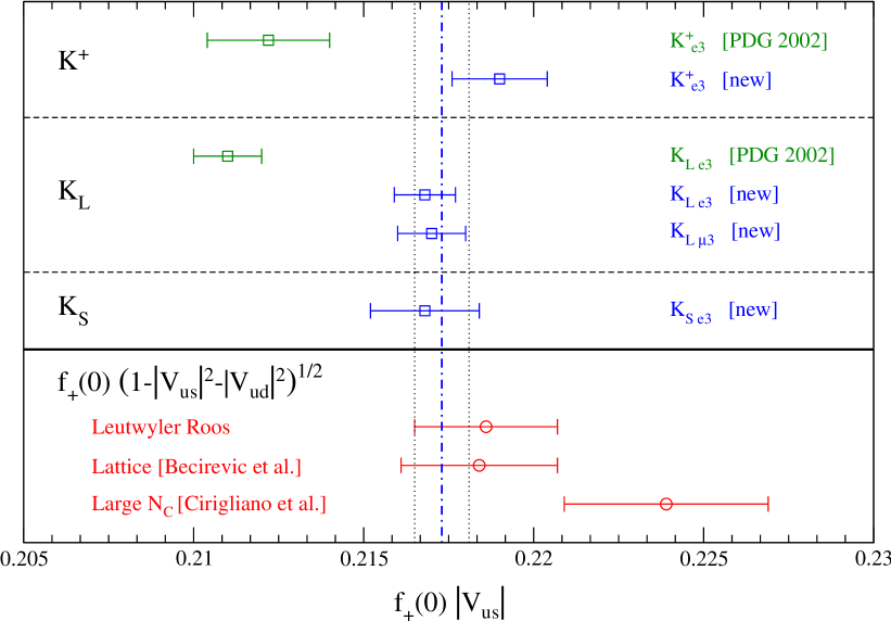
Figure 4: Comparison of the recent measurements of $|V_{us}|f_{+}(0)$ with the PDG 2002 results, and with the expectations of unitarity based on different theoretical calculations of $f_{+}(0)$ [49, 55, 57]. The values of $f_{+}(0)(1-|V_{ud}|^{2}-|V_{ub}|^{2})^{1/2}$ have been obtained using the 2005 value of $V_{ud}$ in Eq. (6); the error bars are largely dominated by the theoretical uncertainty on $f_{+}(0)$. The vertical lines correpsond to the average value of $f_{+}(0)|V_{us}|$ in Eq. (28).

3.3 $V_{us}$ from $K_{\mu 2}$

As recently pointed out in Ref. [76], besides the traditional method of extracting $|V_{us}|$ from $K_{\ell 3}$ decays, one can obtain an independent and competitive estimate of $|V_{us}|$ (or, to be more precise, of $|V_{us}/V_{ud}|$) from the ratio of the inclusive decay widths of ${K^{+}\to\mu^{+}\nu(\gamma)}$ and $\pi^{+}\rightarrow\mu^{+}\nu(\gamma)$ decays. The measurable ratio can be written as follows

$$\frac{\Gamma(K^{+}\to\mu^{+}\nu(\gamma))}{\Gamma(\pi^{+}\to\mu^{+}\nu(\gamma))}=\frac{V_{us}^{2}}{V_{ud}^{2}}\frac{F_{K}^{2}}{F_{\pi}^{2}}\frac{M_{\pi}^{3}(M_{K}^{2}-M_{\mu}^{2})^{2}}{M_{K}^{3}(M_{\pi}^{2}-M_{\mu}^{2})^{2}}\left[1-\frac{\alpha}{\pi}(C_{\pi}-C_{K})\right]~{},$$ (30)

where $F_{K,\pi}$ denote kaon and pion decay constants, and $C_{K,\pi}$ parametrize the radiative-inclusive electroweak corrections, accounting for soft-photon emission and corresponding virtual corrections. According to the detailed analyses of Refs. [78, 79]: $C_{\pi}-C_{K}=3.0\pm 0.75$.

The key theoretical input for this method is the estimate of $F_{K}/F_{\pi}$, obtained by means of lattice QCD. Contrary to the case of $f_{+}(0)$, which is protected by the Ademollo–Gatto theorem, the quantity $[F_{K}/F_{\pi}-1]$ breaks SU(3) invariance already at the first order. It is therefore very challenging to estimate $F_{K}/F_{\pi}$ at the $1\%$ level of accuracy. However, the MILC collaboration has recently shown that this is possible [80]. In 2004 they found $F_{K}/F_{\pi}=1.210\pm 0.014$ [80], value which is compatible with the preliminary result of their new analysis, namely $F_{K}/F_{\pi}=1.198\pm 0.003^{+0.016}_{-0.005}$ [81].

On the experimental side, the dominant error in Eq. (30) is induced by the kaon decay width. KLOE has recently performed a new measurement of the corresponding absolute branching ratio, obtaining $B(K^{+}\to\mu^{+}\nu(\gamma))=0.6366\pm 0.009\pm 0.00015$ [77]. This measurement is fully inclusive of the final state radiation and is based on a sample of $K^{+}$ events tagged by $K^{-}$ decays produced at the $\phi$-meson peak, thus avoiding normalization issues such as trigger and reconstruction efficiency (which enter at first order in the determination of the branching ratio).

Using the new KLOE result, the $K^{+}$ life time from PDG and $V_{ud}=0.9738\pm 0.0003$ (see section 2.1), leads to

$$|V_{us}|_{{K^{+}\to\mu^{+}\nu(\gamma)}} = 0.2223\pm 0.0026\qquad(F_{K}/F_{\pi}=1.210\pm 0.014)~{},$$ (31)

$$|V_{us}|_{{K^{+}\to\mu^{+}\nu(\gamma)}} = 0.2245^{+0.0011}_{-0.0031}\qquad\ \ \ \left(F_{K}/F_{\pi}=1.198\pm 0.003^{+0.016}_{-0.005}\right)~{},$$ (32)

In both cases the error is largely dominated by the uncertainty on $F_{K}/F_{\pi}$ and, in particular, the uncertainty induced by $|V_{ud}|$ is negligible. Both results are consistent with the $V_{us}$ determination from $K_{\ell 3}$.

4 Alternative approaches to $V_{us}$

4.1 $V_{us}$ from hyperon decays: status and perspectives

Hyperon semileptonic decays (HSD), denoted here as $B_{1}\to B_{2}+\ell^{-}+\overline{\nu}_{\ell}$, are described by the $V-A$ theory. This theory states that the weak transitions arise from the self-coupling of a single charged current, which is the sum of the current operators for the leptons and the strongly interacting particles. Each current can be expressed as a linear combination of vector and axial terms. The matrix elements of the lepton current are unambiguous. In contrast, non-perturbative strong interaction effects at low energy weak interactions force the introduction of phenomenological form factors to account for strong interaction effects in the matrix elements. The transition amplitude for HSD can be written as [82]

$${\cal M}_{0}=\frac{G_{F}V_{CKM}}{\sqrt{2}}\,[\overline{u}_{\ell}(l)\gamma^{\mu}(1-\gamma_{5})v_{\nu}(p_{\nu})][\overline{u}_{B_{2}}(p_{2})W_{\mu}u_{B_{1}}(p_{1})],$$ (33)

where $V_{CKM}$ is either $V_{ud}$ or $V_{us}$ and

$$W_{\mu}=f_{1}(q^{2})\gamma_{\mu}+\frac{f_{2}(q^{2})}{M_{1}}\sigma_{\mu\nu}q^{\nu}+\frac{f_{3}(q^{2})}{M_{1}}q_{\mu}+\left[g_{1}(q^{2})\gamma_{\mu}+\frac{g_{2}(q^{2})}{M_{1}}\sigma_{\mu\nu}q^{\nu}+\frac{g_{3}(q^{2})}{M_{1}}q_{\mu}\right]\gamma_{5}.$$ (34)

Here $q\equiv p_{1}-p_{2}$ is the momentum transfer and $M_{1}$ is the mass of the decaying hyperon. The quantities $f_{i}(q^{2})$ and $g_{i}(q^{2})$ are the conventional vector and axial-vector form factors, which are required to be real by time reversal invariance.

The usual approach to evaluate the expected properties of the weak hadronic current is based on the flavor SU(3) symmetry of the strong interactions. In the limit of exact SU(3) symmetry, the hadronic weak currents belong to SU(3) octets, so that the form factors of different HSD are related to each other. The vector part of the weak current and the electromagnetic current belong to the same octet. Thus, the vector form factors are related at $q^{2}=0$ to the electric charge and the anomalous magnetic moments of the nucleons. The conservation of the electromagnetic current implies that $f_{3}(q^{2})$ vanishes for all HSD in the SU(3) limit. Similarly, $g_{1}$ is given in terms of two reduced form factors $F$ and $D$ whereas $g_{2}$ for diagonal matrix elements of hermitian currents vanishes by hermiticity and time-reversal invariance. SU(3) symmetry then implies that $g_{2}=0$ in the symmetry limit.

Currently, experiments in HSD allow precise measurements of form factors (for a review about the experimental situation of HSD see for instance Ref. [83]). The statistical errors of these experiments are rather small, and more effort has been put into the reduction of the systematic errors, which can be of two types. The first one comes from the different shortcomings of the experimental devices. The second one, of theoretical nature, comprises i) radiative corrections and ii) theoretical assumptions for some form factors, including their $q^{2}$ dependence. Let us briefly discuss each one.

The analysis of low, medium, and high-statistics experiments of HSD requires the inclusion of radiative corrections. Since no first principle calculation of radiative corrections is yet possible, these corrections are committed to model dependence and the experimental analyses which use them become model-dependent too. Up to order $(\alpha/\pi)(q/M_{1})$, the model dependence of radiative corrections can be absorbed into the form factors originally defined in the matrix elements of the hadronic current (33) [82] and the remaining part is model independent. Within these orders of approximation one is left with general expressions which can be used in model-independent analyses [84]. Among the integrated observables in HSD, only the decay rates need to be corrected whereas the angular correlations and spin-asymmetry coefficients are practically unaffected [82].

On the other hand, the assumptions on the form factors are subtle to handle. In particular, their $q^{2}$-dependence cannot always be neglected, since noticeable contributions can arise. In order to obtain expressions correct to order ${\mathcal{O}}(q^{2})$, the $q^{2}$-dependence of $f_{2}$ and $g_{2}$ can be ignored, because they already contribute to order ${\mathcal{O}}(q)$ to the decay rate. For $f_{1}(q^{2})$ and $g_{1}(q^{2})$, instead, a linear expansion in $q^{2}$ must be considered, because higher powers amount to negligible contributions to the decay rate. A dipole parametrization of the leading form factors works fine [82].

Another important issue that must be taken into account is the validity of the exact SU(3) limit. Presently, experiments are precise enough that exact SU(3) no longer yields a reliable fit. For HSD, due to the presence of the axial current, SU(3) breaking (SB) can occur in first order. This fact makes HSD to be apparently less reliable to use for determining $V_{us}$ than $K_{l3}$ decays, where the Ademollo-Gatto theorem reduces the effects of SB. For this reason the present value of $V_{us}$ quoted by the Particle Data Group [22] is essentially derived from $K_{l3}$, while the one from HSD is discarded.

Although there are various treatments on the calculation of SB in HSD [85, 86, 87, 88, 89], it is hard to assess their success because their predictions vary substantially from one another and none of them can be considered as fully consistent. These calculations incorporate second-order SB corrections into $f_{1}$. Some computations [85, 86, 87] find that $f_{1}$, for $|\Delta S|=1$ decays, is reduced from its symmetry limit value $f_{1}^{\rm SU(3)}$ such that $f_{1}/f_{1}^{\rm SU(3)}<1$, whereas the calculation of Ref. [88], performed in the framework of Heavy Baryon Chiral Perturbation Theory (HBChPT) [90], found large and positive corrections. Recently, the calculation of SB corrections within HBChPT has been reconsidered in Ref. [89], where it is found that the calculation of [88] contained some mistakes and missed some important contributions. The result of Ref. [89] is that SB corrections, as obtained from HBChPT, are still positive but smaller than previously claimed in [88]. In addition, the quantitative estimate of these corrections strongly depends on the values used for the low energy constants and does not include the contribution coming from the baryon decuplet. This suggests that the corrections coming from higher orders can be large, and that the present estimates may not be reliable. Alternatively, SB effects can be also extracted from the data, for instance parameterising them in the framework of the $1/N_{c}$ expansion of QCD [91, 92, 93, 94].

Fits to the experimental data of HSD to extract $V_{us}$ can be performed using the decay rates and the spin and angular correlation coefficients [22]. There are sufficient data from five decays to make it possible: $\Lambda\to pe^{-}\overline{\nu}_{e}$, $\Sigma^{-}\to ne^{-}\overline{\nu}_{e}$, $\Xi^{-}\to\Lambda e^{-}\overline{\nu}_{e}$, $\Xi^{-}\to\Sigma^{0}e^{-}\overline{\nu}_{e}$, and $\Xi^{0}\to\Sigma^{+}e^{-}\overline{\nu}_{e}$. An alternative set of data is constituted by the decay rates and the measured values of the $g_{1}/f_{1}$ ratios. Since the latter, however, contain less experimental information, using the several angular coefficients instead of $g_{1}/f_{1}$ provides a more sensitive test.

In order to extract $V_{us}$ several analyses can be performed under different assumptions. The analysis done in Ref. [83] neglects the quadratic SB corrections in the vector form factor $f_{1}$ and accounts for the larger effects in the axial form factor $g_{1}$ by using the measured values of the $g_{1}/f_{1}$ ratios of the above processes, except for $\Xi^{-}\to\Sigma^{0}e^{-}\overline{\nu}_{e}$. The matrix element $V_{us}$ is then extracted separately in each decay and the results are combined to obtain the value $V_{us}=0.2250\pm 0.0027$, which is in good agreement with the unitarity requirement.

A similar analysis has been done in Ref. [94], this time using the decay rates and the angular correlation coefficients and performing a global fit to the data of the five decays. By first assuming the validity of exact SU(3) symmetry, the analysis yields $V_{us}=0.2238\pm 0.0019$, with a $\chi^{2}/{\rm dof}$ of around 2.5. This high value of $\chi^{2}$ may signal the presence of not negligible SB corrections. One can proceed further and study the effects upon $V_{us}$ of the leading form factors when SB corrections are taken into account. If one fixes $f_{1}$ at their SU(3) symmetry values and incorporates first-order SB in $g_{1}$ one obtains $V_{us}=0.2230\pm 0.0019$. Next, incorporating SB effects in both $f_{1}$ and $g_{1}$ yields $V_{us}=0.2199\pm 0.0026$ [94]. This analysis also finds that SB corrections to $f_{1}$ increase their magnitudes over their SU(3) symmetric predictions by up to 7% and that corrections to $g_{1}$ are consistent with expectations. This latter $V_{us}$, although in good agreement with the one quoted by the Particle Data Group, does not help in improving the unitarity test. Another interesting finding is that the incorporation of more refined SB corrections systematically reduces the value of $V_{us}$ from its SU(3) symmetric prediction, rather than increasing it to better satisfy unitarity. Of course an increase of $V_{us}$ can be achieved with a symmetry breaking pattern such that $f_{1}/f_{1}^{\rm SU(3)}<1$ [85, 86, 87], but current data do not seem to favour this trend [94].

We are now in a position to make some statements. The first one is that the assumption of exact SU(3) symmetry to compare theory and experiment in HSD is questionable due to the poor fits it produces. The second one is the fact that deviations from the exact SU(3) limit, in particular for the case of the leading axial form factor $g_{1}$, are indeed important to reliably determine $V_{us}$ from HSD, which can rival in precision with the one from $K_{l3}$ decays. Nevertheless more work, theoretical and experimental, is required in the next future to be conclusive about $V_{us}$ from HSD. Particularly, recent techniques in lattice QCD [95] allow to measure form factors with great accuracy, thus determining SB corrections in a model-independent manner.

4.2 Determination of $|V_{us}|$ and $m_{s}$ from hadronic $\tau$ decays

Already over a decade ago, it was realized [97] that hadronic $\tau$ decays provide a very clean testing ground for low energy QCD. For example, analysing the non strange $\tau$ spectral function [96] leads to a determination of the QCD coupling $\alpha_{s}$ that is competitive with the world average. Also, in view of the increasingly precise data on the strange spectral function from ALEPH [98], OPAL [99] and CLEO [100], studying flavor breaking observables allows for a determination of the strange quark mass, another fundamental QCD parameter. The first analyses of this kind [101, 102, 103, 104] were plagued with large uncertainties in the scalar contributions due to a bad behavior of the associated perturbation series. This problem was circumvented [105] by substituting the theoretical expressions with phenomenological counterparts, thereby reducing the theoretical uncertainties significantly. Along with this procedure, it was realized that the main uncertainty in the strange quark mass determination was now arising from the uncertainty in the CKM parameter $|V_{us}|$, which suggests [105, 106] to turn the analysis around and determine $|V_{us}|$.

The basic objects for a QCD analysis of hadronic $\tau$ decays are the two point correlation functions for vector $V^{\mu}_{ij}\equiv\overline{q}_{i}\gamma^{\mu}q_{j}$ and axial-vector $A^{\mu}_{ij}\equiv\overline{q}_{i}\gamma^{\mu}\gamma_{5}q_{j}$ currents. Both correlation functions contain (pseudo)scalar and (axial) vector contributions. Then, the ratio of hadronic to leptonic $\tau$ decay rates

$$R_{\tau}\equiv\frac{\Gamma\left[\tau^{-}\to{\rm hadrons}(\gamma)\right]}{\Gamma\left[\tau^{-}\to e^{-}\overline{\nu}_{e}\nu_{\tau}(\gamma)\right]},$$ (35)

as well as higher moments of the invariant mass distribution

$$R_{\tau}^{(k,l)}\equiv{\displaystyle\int^{M_{\tau}^{2}}_{0}}{\rm d}s\left(1-\frac{s}{M_{\tau}^{2}}\right)^{k}\,\left(\frac{s}{M_{\tau}^{2}}\right)^{l}\,\frac{{\rm d}R_{\tau}}{{\rm d}s}$$ (36)

can be calculated in an operator product expansion:

$$R_{\tau}^{(k,l)}\equiv N_{c}S_{\rm EW}\Big{\{}(|V_{ud}|^{2}+|V_{us}|^{2})\,\left[1+\delta^{(k,l)(0)}\right]$$

$$+{\displaystyle\sum_{D\geq 2}}\left[|V_{ud}|^{2}\delta^{(k,l)(D)}_{ud}+|V_{us}|^{2}\delta^{(k,l)(D)}_{us}\right]\Big{\}}\,.$$ (37)

Here, $S_{EW}=1.0201\pm 0.0003$ summarizes electroweak radiative corrections, while explicit expressions for the $\delta^{(k,l)(D)}_{ij}$ and additional theoretical information can be found in [101] as well as references therein. The dominant contribution to $R_{\tau}$ is purely perturbative and summarized in $\delta^{(k,l)(0)}$, while higher dimensional contributions that also depend on the flavor content are suppressed. The most important of these suppressed terms are proportional to $m_{s}^{2}$ and $m_{s}\langle\overline{q}q\rangle$. To reduce perturbative uncertainties one conveniently discusses the flavor breaking observable

$$\delta R^{(k,l)}_{\tau}\equiv\frac{R^{(k,l)}_{\tau,V+A}}{|V_{ud}|^{2}}-\frac{R^{(k,l)}_{\tau,S}}{|V_{us}|^{2}}=N_{c}\,S_{EW}\,{\displaystyle\sum_{D\geq 2}}\left[\delta^{(k,l)(D)}_{ud}-\delta^{(k,l)(D)}_{us}\right]\,,$$

where the definition of the flavour-dependent moments $R^{(k,l)}_{\tau,V+A}$ and $R^{(k,l)}_{\tau,S}$ can be found in Ref. [105]. In this expression, the main parametric uncertainties arise only from $m_{s}$ and $|V_{us}|$, so that one could ideally determine both parameters simultaneously from the experimental analysis of several moments (see [105] for more details). In absence of such an analysis, we proceed as in [106] and begin by determining $|V_{us}|$ from the moment with the smallest dependence on $m_{s}$, i.e. the (0,0) moment. Using $m_{s}(2{\rm GeV})=(95\pm 20)$ MeV (in the the $\overline{MS}$ scheme), in agreement with recent sum rule and lattice calculations, one finds $\delta R_{\tau,\rm th}^{(0,0)}=0.218\pm 0.026$, and, with

$$|V_{us}|^{2}=\frac{R^{(0,0)}_{\tau,S}}{\frac{\displaystyle R^{(0,0)}_{\tau,V+A}}{\displaystyle|V_{ud}|^{2}}-\delta R^{(0,0)}_{\tau,{\rm th}}}$$ (38)

one obtains

$$|V_{us}|=0.2208\pm 0.0033_{\rm exp}\pm 0.0009_{\rm th}=0.2208\pm 0.0034,$$ (39)

where we have used $R^{(0,0)}_{\tau,V+A}=3.469\pm 0.014$ and $R^{(0,0)}_{\tau,S}=0.167\pm 0.0050$ from [99]. The most important feature of this determination is the small theoretical uncertainty, the reason for which can nicely be seen from Eq. (38): the large cancellations between strange and non strange channels lead to a small value of $\delta R^{(0,0)}_{\tau,{\rm th}}$, so that the main sensitivity is to the experimental input. It is also interesting to check whether this value of $|V_{us}|$ is compatible with unitarity: using the value $|V_{ud}|=0.9739\pm 0.0003$ (see section 2), one finds that Eq. (1) is violated only at the 1.8 $\sigma$ level.

In the next step, one uses the value of $|V_{us}|$ thus obtained and determines the strange quark mass from higher moments. One finds the values given in Table 5, where the individual sources of the uncertainties are given in [106].

Moment	(2,0)	(3,0)	(4,0)
$m_{s}(M_{\tau})$ MeV	$93.2^{+34}_{-44}$	$86.3^{+25}_{-30}$	$79.2^{+21}_{-23}$

Table 5: Results for $m_{s}(M_{\tau})$ extracted from the different moments.

The weighted average of the strange mass values obtained for the different moments give

$$m_{s}(M_{\tau}^{2})=84\pm 23\,{\rm MeV}\,\Rightarrow m_{s}(2{\rm GeV})=81\pm 22\,{\rm MeV}\ ,$$ (40)

in good agreement with the average given above, while a more detailed comparison can be found in [106]. The values of $m_{s}$ display a monotonous $k$ dependence, which has been significantly reduced with the new OPAL data, mainly due to the new value for the $B(\tau^{-}\to K^{-}\pi^{+}\pi^{-}\nu)$ branching ratio.

In summary, the $\left|V_{us}\right|$ value obtained from $\tau$ decays is beginning to become competitive with the standard determination from $K$ decays and is given in Eq. (39). In particular, due to the fact that the largest amount of the uncertainty is still experimental, one can expect that the better data samples from BaBar and Belle will reduce this uncertainty significantly. In view of these perspectives it will be important to have the possibility to determine both $m_{s}$ and $|V_{us}|$ simultaneously. An analysis of this type is underway. Additionally, further, precise data will clarify whether the moment dependence of the $m_{s}$ results is indeed a purely experimental issue, and thereby allow a consistency check of the whole analysis.

5 Future prospects on $V_{cs}$ and $V_{cd}$

5.1 Theoretical developments

As far as the extraction of $V_{cs}$ and $V_{cd}$ is concerned, the most interesting recent developments are the lattice QCD calculations of the matrix elements for semileptonic and leptonic $D_{(s)}$ decays. With the advent of dynamical simulations with light sea quarks, decays to $K$ and $\pi$ mesons are favoured because the final-state particles are stable to strong decay. The headline results have come from simulations using $2{+}1$ flavours of improved staggered light quarks where the common light ($u$, $d$) quark mass is in the range $m_{s}/8<m_{\mathrm{light}}<3m_{s}/4$. The “fourth root trick” used in generating these dynamical configurations has not been completely justified theoretically, but on the other hand it has not so far failed any test. There is a requirement to deal with the unphysical “tastes” introduced, but this has been addressed by the development of staggered chiral perturbation theory (S$\chi$PT) [107, 108], allowing the subtraction of discretisation effects arising from light quark taste violations.

5.1.1 Lattice Results for Semileptonic $D$ Decays

For semileptonic $D$ decays to a light final state pseudoscalar or vector meson, $P$ or $V$, the squared momentum transfer is $q^{2}=m_{D}^{2}+m_{P,V}^{2}-2m_{D}E$ where $E$ is the $P$ or $V$ energy in the $D$ rest frame. In lattice simulations, the entire range, $0\leq q^{2}\leq(m_{D}-m_{P,V})^{2}=q^{2}_{\mathrm{max}}$, can be accessed while keeping the initial and final state meson spatial momenta small enough to avoid large discretisation effects.

Two form factors, $f_{+}(q^{2})$ and $f_{0}(q^{2})$ are needed to describe the vector current matrix element for semileptonic decays to a light pseudoscalar, but only $f_{+}(q^{2})$ is needed for the decay rate if the lepton mass can be ignored. Lattice QCD gives results for both form factors and this can be helpful since they can be fit simultaneously imposing the constraint $f_{+}(0)=f_{0}(0)$.

The Fermilab-MILC-HPQCD collaboration has reported results for semileptonic $D\to K$ and $D\to\pi$ decays using $2{+}1$ flavours of improved staggered quarks [109, 110]. The charm quark is implemented using the Fermilab method [111], while the calculations are so far performed at one lattice spacing. Indeed, the dominant systematic effect comes from the heavy quark discretisation error, estimated from the mismatch of the continuum and lattice heavy quark effective theories [112, 113] and comprising $7\%$ of the $10\%$ total systematic error in the form factors.

It is convenient to perform the chiral extrapolations at fixed pion energy, $E$. To do this, the form factors for different light quark masses are fit to the Becirevic-Kaidalov (BK) parametrisation [114], which satisfies $f_{+}(0)=f_{0}(0)$, obeys heavy quark scaling relations near zero recoil ($q^{2}_{\mathrm{max}}$) and at $q^{2}=0$ and contains a $D^{*}_{(s)}$ pole in $f_{+}$. They are then interpolated to a common set of fixed values of $E$ and extrapolated using the S$\chi$PT expressions [107, 108]. After this, $f_{+,0}$ are recovered and a final BK fit is made to extend the results to the full kinematic range. The output form factors are shown in figure 5 and compared to FOCUS results [116] for $f_{+}^{D\to K}$. Results for $f_{+}(0)$, compared to quenched calculations, are:

$$\begin{array}[]{rll}&N_{f}=0&N_{f}=2{+}1\\ f_{+}^{D\to\pi}(0)&0.62(7)&0.64(3)(6)\\ f_{+}^{D\to K}(0)&0.71(8)&0.73(3)(7)\\ f_{+}^{D\to\pi}(0)/f_{+}^{D\to K}(0)&&0.87(3)(9)\end{array}$$

The quenched results are an average from [117, 118, 119, 120, 121, 122], with an added $10\%$ error incorporated to allow for unquenching and lack of a continuum extrapolation.

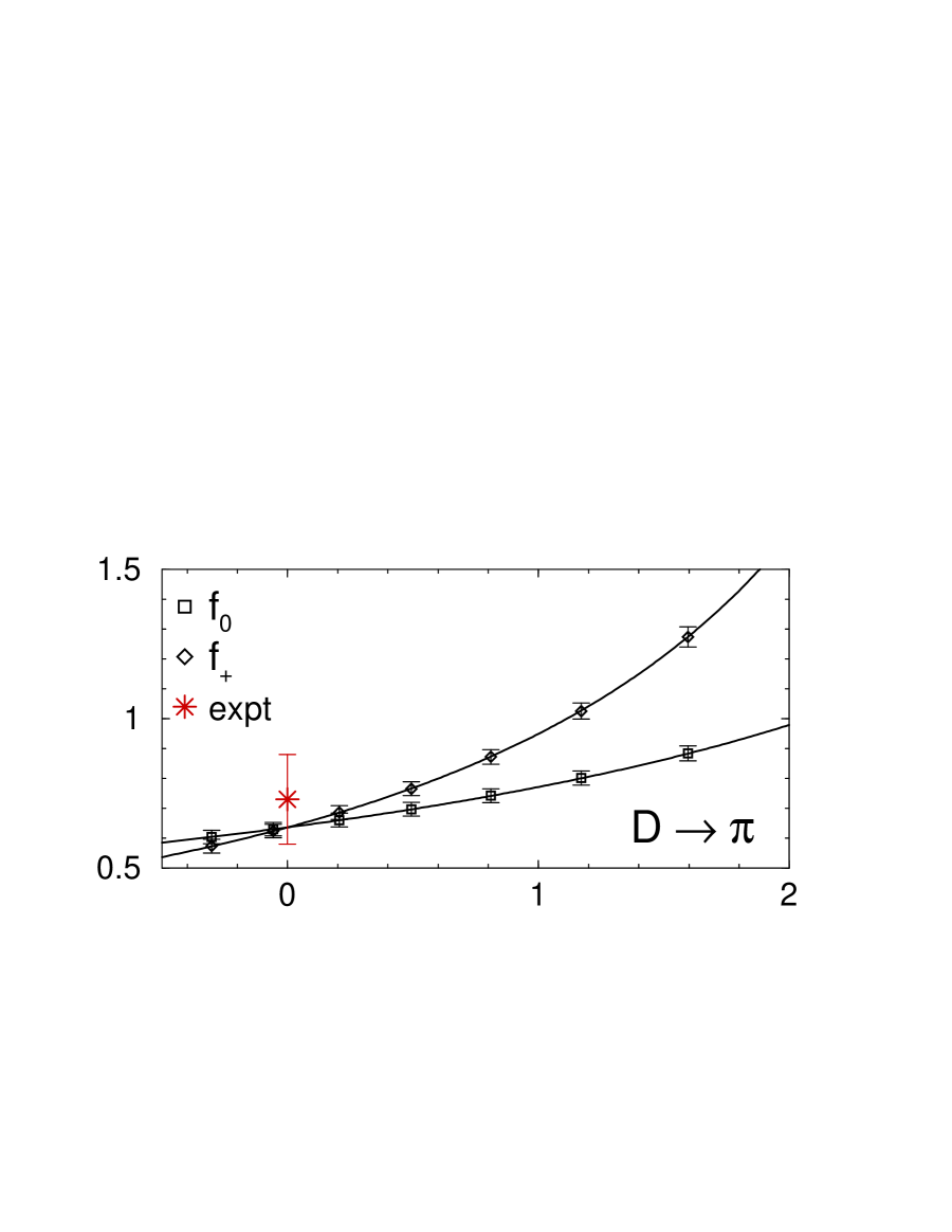
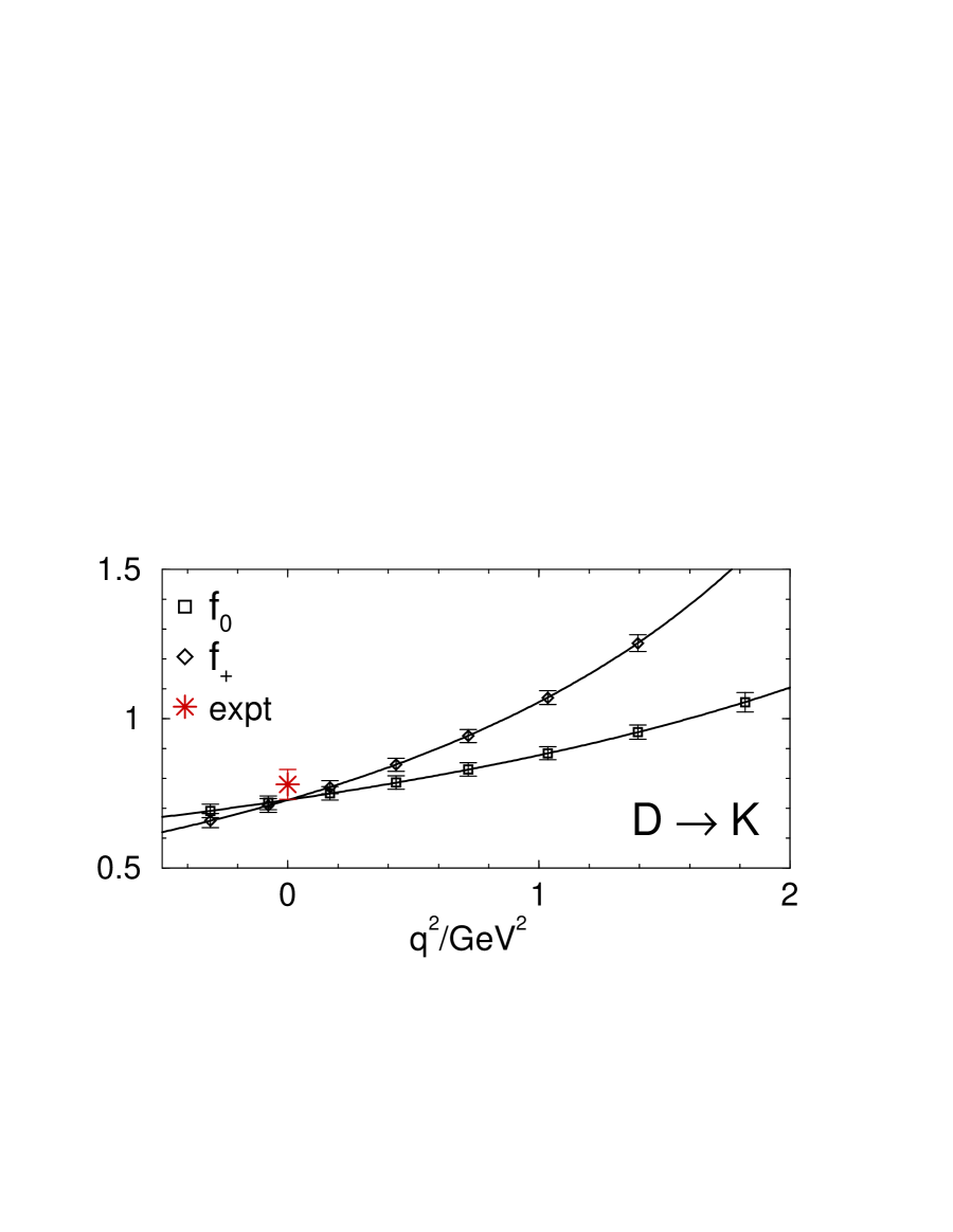
Figure 5: Left: Fermilab-MILC-HPQCD results [109] for $D\to\pi$ and $D\to K$ semileptonic decay form factors. The experimental points at $q^{2}=0$ are from BES [123]. Right: comparison of FNAL-MILC-HPQCD calculation [109] of $f_{+}$ for $D\to Kl\nu$ with FOCUS data [116]. The green curve is a fit to the BK parametrisation using the lattice data. The green triangles show $q^{2}$ values where the fixed-$E$ chiral extrapolation ends up. The green curve and points use the central values of the fitted BK parameters. The blue points are from FOCUS.

For decays to light vector mesons, only quenched results are available. The most recent results for $D\to K^{*}l\nu$ come from the SPQcdR collaboration [124]. There are four form factors, $V$ and $A_{0,1,2}$, but $A_{0}$ is not needed for the decay rate. $A_{2}$ is the least well determined, but since it is common to quote values at $q^{2}=0$, $A_{2}(0)$ can be determined from $A_{0}(0)$ and $A_{1}(0)$. Combining the SPQcdR results at their finer lattice spacing with previous results from [117, 118, 120, 121], gives:

$$V(0)=1.17(14),\qquad A_{1}(0)=0.69(7),\qquad A_{2}(0)=0.58(8).$$

SPQcdR fit their form factors to pole/dipole ansätze (consistent with heavy quark scaling laws) and then integrate to find [124] (at their finer lattice spacing):

$$\Gamma(D^{-}\to K^{*0}l\nu)/|V_{cs}^{2}|=0.062(15)\,\mathrm{ps}^{-1}$$

5.1.2 Lattice Results for $f_{D_{s}}$ and $f_{D}$

Figure 6: History of $f_{D_{s}}$ calculations in lattice QCD (adapted from plot shown by Hashimoto [138] at ICHEP04). The shaded background shows the Particle Data Group [22] experimental world average $f_{D_{s}}=(267\pm 33)\,\mathrm{Me\kern-0.89996ptV}$, with $|V_{cs}|$ as input.

Recent quenched lattice results for $D$-meson decay constants have concentrated on controlling all systematic errors save for quenching itself [130, 131]. Attention has now shifted to simulations with dynamical quarks [126, 127, 139, 140]. Figure 6 shows results from lattice calculations of $f_{D_{s}}$ published from 1998 onwards.

Dynamical simulations with two clover flavours of light quark (although with $m_{\mathrm{sea}}>m_{s}/2$) are in progress [127]. Simulations using $2{+}1$ flavours of improved staggered quarks currently allow the lightest sea quark masses to be reached. In one case [126], the heavy quark is treated using NRQCD and the extrapolation to the $D_{s}$ meson tends to magnify errors. The Fermilab-MILC-HPQCD collaboration treat the charm quark directly and use a large set of valence and sea quark masses to help control the chiral extrapolation [140, 125]. A fit using S$\chi$PT [107] allows discretisation errors from staggering to be removed. For $f_{D_{s}}$, the valence quark mass is interpolated to the strange mass, and then the sea quark mass is extrapolated to the up–down mass. In contrast, for $f_{D}$, the valence and sea masses are set equal and extrapolated together. The results are [125]:

$$\begin{array}[]{rcl}f_{D_{s}}&=&249(3)(16)\,\mathrm{Me\kern-0.89996ptV}\\ f_{D}&=&201(3)(17)\,\mathrm{Me\kern-0.89996ptV}\end{array}$$

5.1.3 Sumrule Results

Sumrules are generally less stable for $D$ mesons than for $B$ mesons: there are larger higher order operator and perturbative corrections. For the semileptonic decays of $D$ mesons to $\pi$ or $K$ mesons, Khodjamirian is updating the lightcone sumrule predictions [141] using an updated value for the charm quark mass, $m_{c}=1.46\pm 0.1\,\mathrm{Ge\kern-0.89996ptV}$ [22], and new Gegenbauer moments for the kaon and pion distribution amplitudes [142]. The preliminary results, compared to the summary [143] from the 2003 CKM workshop, are:

$$\begin{array}[]{rll}&\mbox{CKM03~{}\cite[cite]{[\@@bibref{}{Khodjamirian:2003rf}{}{}]}}&\mbox{2005~{}\cite[cite]{[\@@bibref{}{kho-lcsr2005}{}{}]}}\\ f^{D\to\pi}_{+}(0)&0.65(11)&0.61(11)\\ f^{D\to K}_{+}(0)&0.78(11)&0.79(14)(8)\\ f^{D\to\pi}_{+}(0)/f^{D\to K}_{+}(0)&&0.77(4)(8)\end{array}$$

The second error in $f_{+}^{D\to K}$ arises from variation in the strange quark mass, $m_{s}=130\mp 20\,\mathrm{Me\kern-0.89996ptV}$.

For the decay constants, the summary from the 2003 CKM workshop still stands [143]:

$$f_{D}=200\pm 20\,\mathrm{Me\kern-0.89996ptV},\qquad f_{D_{s}}/f_{D}=1.11\mbox{\ to\ }1.27$$

5.2 Recent experimental results on charm decays

Precision measurements of semileptonic charm decay rates and form factors are a principal goal of the CLEO-c program at the Cornell Electron Storage Ring (CESR)[145]. We review herein measurements with the first CLEO-c data of the absolute branching fractions of $D^{0}$ decays to $K^{-}e^{+}\nu_{e}$, $\pi^{-}e^{+}\nu_{e}$ and $K^{*-}e^{+}\nu_{e}$, as well as of $D^{+}$ decays to $\bar{K}^{0}e^{+}\nu_{e}$, $\pi^{0}e^{+}\nu_{e}$, $\bar{K}^{*0}e^{+}\nu_{e}$ and $\rho^{0}e^{+}\nu_{e}$, including the first observations and absolute branching fraction measurements of $D^{0}\rightarrow\rho^{-}e^{+}\nu_{e}$ and $D^{+}\rightarrow\omega e^{+}\nu_{e}$ [146, 147], and compare them to recent measurements from other experiments and theoretical predictions. We also review the prospects for measuring semileptonic form factors and the CKM matrix elements $V_{cs}$ and $V_{cd}$ with the full CLEO-c data set.

The data for this analysis were collected by the CLEO-c detector at the $\psi(3770)$ resonance, about 40 MeV above the $D\bar{D}$ pair production threshold. A description of the CLEO-c detector is provided in Ref. [146] and references therein. The data sample consists of an integrated luminosity of 55.8 pb^-1 and includes about 160,000 $D^{+}D^{-}$ and 200,000 $D^{0}\bar{D}^{0}$ events.

The technique for these measurements was first applied by the Mark III collaboration [148] at SPEAR. Candidate events are selected by reconstructing a $\bar{D}^{0}$ ($D^{-}$), called a tag, in a hadronic final state. The absolute branching fractions of $D^{0}$ ($D^{+}$) semileptonic decays are then measured by their reconstruction in the system recoiling from the tag. Tagging a $\bar{D}^{0}$ ($D^{-}$) meson in a $\psi(3770)$ decay provides a $D^{0}$ ($D^{+}$) with known four-momentum, allowing a semileptonic decay to be reconstructed with no kinematic ambiguity, even though the neutrino is undetected.

Tagged events are selected based on two variables: $\Delta E\equiv E_{D}-E_{\rm beam}$, the difference between the energy of the $D^{-}$ tag candidate ($E_{D}$) and the beam energy ($E_{\rm beam}$), and the beam-constrained mass $M_{\rm bc}\equiv\sqrt{E_{\rm beam}^{2}/c^{4}-|\vec{p}_{D}|^{2}/c^{2}}$, where $\vec{p}_{D}$ is the measured momentum of the $D^{-}$ candidate [149]. If multiple candidates are present in the same tag mode, one candidate per $\bar{D}^{0}$ or $D^{-}$ is chosen using $\Delta E$, and the yields in each tag modes are obtained from fits to the $M_{\rm bc}$ distributions. The data sample comprises approximately 60,000 (32,000) neutral (charged) tags, reconstructed in eight neutral (six charged) $D$ meson hadronic final states [146, 147], respectively.

After a tag is identified, the positron and a set of hadrons recoiling against the tag is searched for. (Muons are not used as $D$ semileptonic decays at the $\psi(3770)$ produce low momentum leptons for which the CLEO-c muon identification is not efficient.) The efficiency for positron identification rises from about $50\%$ at 200 MeV/$c$ to 95% just above 300 MeV/$c$ and is roughly constant thereafter, while the positron fake rate from charged pions and kaons is approximately 0.1% [146]. Candidates for $\pi^{0}$ are identifid from photon pairs, each having an energy of at least 30 MeV, with invariant mass within 3.0$\sigma$ ($\sigma\sim 6$ ${\rm MeV}/c^{2}$) of the known $\pi^{0}$ mass. The $K^{0}_{S}$ candidates are formed from pairs of oppositely-charged and vertex-constrained tracks having an invariant mass within 12 MeV/$c^{2}$ $(\sim 4.5\sigma)$ of the known $K^{0}_{S}$ mass. $\bar{K}^{*-}$/$\rho^{-}$/$\bar{K}^{*0}$/$\rho^{0}$ candidates are formed from ($K^{-}$ and $\pi^{0}$) or ($K^{0}_{S}$ and $\pi^{-}$) / ($\pi^{-}$ and $\pi^{0}$) / ($K^{-}$ and $\pi^{+}$) / ($\pi^{-}$ and $\pi^{+}$) combinations and require an invariant mass within 100 MeV/$c^{2}$ and 150 MeV/$c^{2}$ for the $K^{*}$ and $\rho$ from the expected mean values. The reconstruction of $\omega\rightarrow\pi^{+}\pi^{-}\pi^{0}$ candidates is achieved by combining three pions, requiring an invariant mass within 20 MeV/$c^{2}$ of the known mass, and demanding that the charged pions do not satisfy interpretation as a ${K}^{0}_{S}$.

The tag and the semileptonic decay are then combined, if the event includes no tracks other than those of the tag and the semileptonic candidate. Semileptonic decays are identified using the variable $U\equiv E_{\rm miss}-|\vec{p}_{\rm miss}|c$, where $E_{\rm miss}$ and $\vec{p}_{\rm miss}$ are the missing energy and momentum of the $D$ meson decaying semileptonically. If the decay products of the semileptonic decay have been correctly identified, $U$ is expected to be zero, since only a neutrino is undetected. The $U$ distribution has $\sigma\sim 10~{}{\rm MeV}$. (The width varies by mode and is larger for modes with $\pi^{0}$ mesons.) To remove multiple candidates in each semileptonic mode, one combination is chosen per tag mode, based on the proximity of the invariant masses of the $K_{S}^{0}$, $\bar{K}^{*}$, $\rho$, $\pi^{0}$, or $\omega$ candidates to their expected masses.

The new results for the branching ratios of various semileptonic modes are reported in Table 6. For each mode the yield is determined from a fit to its $U$ distribution. The backgrounds are generally small and arise mostly from misreconstructed semileptonic decays with correctly reconstructed tags. The absolute branching fractions are then determined using ${\cal B}={N_{\rm signal}/\epsilon N_{\rm tag}}$, where $N_{\rm signal}$ is the number of fully reconstructed $D\bar{D}$ events obtained by fitting the $U$ distribution, $N_{\rm tag}$ is the number of events with a reconstructed tag, and $\epsilon$ is the effective efficiency for detecting the semileptonic decay in an event with an identified tag.

Mode	Yield	$\mathcal{B}$ (%)	$\mathcal{B}$ (%) (PDG)
$D^{0}\rightarrow K^{-}e^{+}\nu_{e}$	$1311\pm 37$	$3.44\pm 0.10\pm 0.10$	$3.58\pm 0.18$
$D^{0}\rightarrow\pi^{-}e^{+}\nu_{e}$	$116.8\pm 11.2$	$0.26\pm 0.03\pm 0.01$	$0.36\pm 0.06$
$D^{0}\rightarrow K^{*-}e^{+}\nu_{e}$	$219.3\pm 15.6$	$2.16\pm 0.15\pm 0.08$	$2.15\pm 0.35$
$D^{0}\rightarrow\rho^{-}e^{+}\nu_{e}$	$31.1\pm 6.3$	$0.19\pm 0.04\pm 0.01$	—
$D^{+}\rightarrow\bar{K}^{0}e^{+}\nu_{e}$	$545\pm 24$	$8.71\pm 0.38\pm 0.37$	$6.7\pm 0.9$
$D^{+}\rightarrow\pi^{0}e^{+}\nu_{e}$	$63.0\pm 8.5$	$0.44\pm 0.06\pm 0.03$	$0.31\pm 0.15$
$D^{+}\rightarrow\bar{K}^{*0}e^{+}\nu_{e}$	$422\pm 21$	$5.56\pm 0.27\pm 0.23$	$5.5\pm 0.7$
$D^{+}\rightarrow\rho^{0}e^{+}\nu_{e}$	$27.4\pm 5.7$	$0.21\pm 0.04\pm 0.01$	$0.25\pm 0.10$
$D^{+}\rightarrow\omega e^{+}\nu_{e}$	$7.6^{+3.3}_{-2.7}$	$0.16^{+0.07}_{-0.06}\pm 0.01$	—

Table 6: Signal yields and branching fractions as recently obtained at CLEOc vs. the PDG results [22]. The first uncertainty is statistical and the second systematic in the third column, and statistical or total in the other columns. The yield ($\mathcal{B}$) for $D^{0}\rightarrow K^{*-}e^{+}\nu_{e}$ is summed (averaged) over the two $K^{*-}$ submodes of $K^{-}\pi^{0}$ and $K^{0}_{S}\pi^{-}$. Signal yields for $D^{0}\rightarrow\rho^{-}e^{+}\nu_{e}$ and $D^{+}\rightarrow\omega e^{+}\nu_{e}$ are significant and represent the first observations of these modes.

The largest contributors to the systematic uncertainty are associated with the tracking efficiency, the $\pi^{0}$ and $K_{S}^{0}$ reconstruction efficiencies, the extraction of $D$ tag yields, the positron and hadron identification efficiencies, background shapes and normalizations, imperfect knowledge of form factors, and the simulation of final state radiation. The non-resonant contribution in the $D\rightarrow K^{*}e\nu_{e}$ reconstruction and the associated systematic uncertainty are accounted for as described in Ref. [146, 147]. The total systematic uncertainty ranges from 2.8% to 7.8% according to the mode. Most systematic uncertainties are measured in data and will be reduced with a larger data set.

The widths of the isospin conjugate exclusive semileptonic decay modes of the $D^{0}$ and $D^{+}$ are related by isospin invariance of the hadronic current. The ratio $\frac{\Gamma(D^{0}\rightarrow K^{-}e^{+}\nu_{e})}{\Gamma(D^{+}\rightarrow\bar{K}^{0}e^{+}\nu_{e})}$ is expected to be unity. The world average value is $1.35\pm 0.19$ [22]. Using the new results and the lifetimes of the $D^{0}$ and $D^{+}$ [22], one obtains: $\frac{\Gamma(D^{0}\rightarrow K^{-}e^{+}\nu_{e})}{\Gamma(D^{+}\rightarrow\bar{K}^{0}e^{+}\nu_{e})}=1.00\pm 0.05{\rm(stat)}\pm 0.04{\rm(syst)}.$ The result is consistent with unity and with two recent less precise results: a measurement from BES II using the same technique [150] and an indirect measurement from FOCUS [151, 152]. The ratios of isospin conjugate decay widths for other semileptonic decay modes are given in Ref. [147] and are all consistent with isospin invariance.

As the data are consistent with isospin invariance, the precision of each branching fraction can be improved by averaging the $D^{0}$ and $D^{+}$ results for isospin conjugate pairs. The isospin-averaged semileptonic decay widths, with correlations among systematic uncertainties taken into account, are given in Table 7.

Decay Mode	$\Gamma$ ($10^{-2}\times{\rm ps}^{-1}$)
$D\rightarrow K\;e^{+}\nu_{e}$	$8.38\pm 0.20\pm 0.23$
$D^{0}\rightarrow\pi^{-}e^{+}\nu_{e}$	$0.68\pm 0.05\pm 0.02$
$D\rightarrow K^{*}\;e^{+}\nu_{e}$	$5.32\pm 0.21\pm 0.20$
$D^{0}\rightarrow\rho^{-}e^{+}\nu_{e}$	$0.43\pm 0.06\pm 0.02$

Table 7: Isospin-averaged semileptonic decay widths with statistical and systematic uncertainties. For Cabibbo-suppressed modes, the isospin average is calculated for the $D^{0}$ using $\Gamma(D^{0})=2\times\Gamma(D^{+})$.

The ratio of decay widths for $D\rightarrow\pi e^{+}\nu$ and $D\rightarrow Ke^{+}\nu$ provides a test of the LQCD charm semileptonic rate ratio prediction [153]. Using the results in Table 7, one finds $\frac{\Gamma(D^{0}\rightarrow\pi^{-}e^{+}\nu)}{\Gamma(D\rightarrow Ke^{+}\nu)}=(8.1\pm 0.7{\rm(stat)}\pm 0.2{\rm(syst)})\times 10^{-2}$, consistent with LQCD and two recent results [154, 155]. Furthermore, the ratio $\frac{\Gamma(D\rightarrow K^{*}e^{+}\nu)}{\Gamma(D\rightarrow Ke^{+}\nu)}$ is predicted to be in the range 0.5 to 1.1 (for a compilation see Ref. [151]). Using the isospin averages in Table 7, one finds $\frac{\Gamma(D\rightarrow K^{*}e^{+}\nu)}{\Gamma(D\rightarrow Ke^{+}\nu)}=0.63\pm 0.03{\rm(stat)}\pm 0.02{\rm(syst)}$.

The modest in size data sample used in this analysis produced the most precise measurements to date of the absolute branching fractions for all modes in Table 6. The analysis already provides stringent tests of the theory. This precision is consistent with the expected performance of CLEO-c. CESR is running to collect a much larger $\psi(3770)$ data sample.

The future CLEO-c data sample (3.0 fb^-1) will allow measurements of the $q^{2}$ dependence ($f_{+}(q^{2})$) and, assuming the unitarity of the CKM matrix, the absolute normalization ($f_{+}(0)$) of form factors at a percent level ($\mathcal{O}(1\%)$) in both $D\rightarrow Ke^{+}\nu_{e}$ and $D\rightarrow\pi e^{+}\nu_{e}$ [145]. For $D\rightarrow K^{*}e^{+}\nu_{e}$ and $D\rightarrow\rho e^{+}\nu_{e}$, form factors $A_{1}(q^{2})$, $A_{2}(q^{2})$, and $V(q^{2})$ can be measured to a few percent [145]. These measurements of form factors (and other precision measurements in the $D$, $B$, $\Upsilon$ and $\psi$ systems) constitute calibration and validation data for LQCD and other theoretical approaches.

Theoretical predictions for form factors are required for measurements of the CKM matrix elements. In charm decays, the modes $D^{0}\rightarrow K^{-}e^{+}\nu_{e}$ and $D^{0}\rightarrow\pi^{-}e^{+}\nu_{e}$ are important as they are the simplest for both theory and experiment. Assuming future theoretical uncertainties on the form factors in these decays of 3.0% and using the anticipated uncertainties for the absolute decay rates of $D^{0}\rightarrow K^{-}e^{+}\nu_{e}$ and $D^{0}\rightarrow\pi^{-}e^{+}\nu_{e}$ from CLEO-c of 1.2% and 1.5%, respectively, the following uncertainties on $|V_{cs}|$ and $|V_{cd}|$ are within reach: $|\sigma(V_{cs})/V_{cs}|\approx 1.6\%$ and $|\sigma(V_{cd})/V_{cd}|\approx 1.7\%$ [145].

6 Conclusions

As discussed in section 2, at present the determination of $|V_{ud}|$ is largely dominated by super-allowed, $0^{+}\rightarrow 0^{+}$ nuclear beta decays. Taking into account the new theoretical analysis of radiative corrections in Ref. [9], and the new global fit by Savard et al. [11], leads to

$$|V_{ud}|=0.97377\pm 0.00027~{}.$$ (41)

Hopefully, in the near future a competitive independent information on $|V_{ud}|$ will be extracted from the neutron beta decay, once the experimental situation on the neutron lifetime will be clarified.

Concerning $V_{us}$, at present the most reliable determination is the one obtained by means of $K_{\ell 3}$ decays –see Eq. (28)– employing the Leutwyler-Roos value of $f_{+}(0)$ [49], which is supported by several recent lattice results [57, 59, 60, 61, 62]:

$$|V_{us}|_{K_{\ell 3}}=0.2261\pm 0.0021\qquad\left[f_{+}(0)=0.961\pm 0.008\right]~{}.$$ (42)

Of comparable accuracy is the value extracted from the $\Gamma(K_{\mu 2})/\Gamma(\pi_{\mu 2})$ ratio, employing the updated lattice result of $F_{K}/F_{\pi}$ [81]:

$$|V_{us}|_{K_{\mu 2}}=0.2245^{+0.0011}_{-0.0031}\qquad\left[F_{K}/F_{\pi}=1.198\pm 0.003^{+0.016}_{-0.005}\right]~{}.$$ (43)

The average of these two values leads to

$$|V_{us}|_{K~{}{\rm decays}}=0.225\pm 0.001~{},$$ (44)

which can be considered as the final global estimate of $V_{us}$.

Using the values in Eqs. (41) and (44) the unitarity relation in Eq. (1) is satisfied within $1\sigma$ at the $10^{-3}$ level:

$$\Delta=1-\left(|V_{ud}|^{2}+|V_{us}|^{2}+|V_{ub}|^{2}\right)=(1\pm 1)\times 10^{-3}~{}.$$ (45)

References

- [1] N. Cabibbo, Phys. Rev. Lett. 1̱0 (1963) 531.
- [2] M. Kobayashi and T. Maskawa, Prog. Th. Phys 49 (1973) 652.
- [3] R. E. Behrends and A. Sirlin, Phys. Rev. Lett. 4 (1960) 186.
- [4] M. Ademollo and R. Gatto, Phys. Rev. Lett. 13 (1964) 264.
- [5] A. Sirlin, Rev. Mod. Phys. 50, 573 (1978) [Erratum-ibid. 50, 905 (1978)].
- [6] A. Czarnecki, W. J. Marciano and A. Sirlin, Phys. Rev. D 70, 093006 (2004) [hep-ph/0406324].
- [7] I. S. Towner and J. C. Hardy, Phys. Rev. C 66, 035501 (2002) [nucl-th/0209014].
- [8] W. J. Marciano and A. Sirlin, Phys. Rev. Lett. 56, 22 (1986).
- [9] W. J. Marciano and A. Sirlin, hep-ph/0510099.
- [10] J. C. Hardy and I. S. Towner, Phys. Rev. Lett. 94, 092502 (2005) [nucl-th/0412050].
- [11] G. Savard et al., Phys. Rev. Lett. 95, 102501 (2005).
- [12] H. Abele, D. Mund, eds. Proceedings of Quark-Mixing, CKM-Unitarity, Heidelberg, Sep 2002, Mattes-Verlag, Heidelberg (2003).
- [13] D. H. Wilkinson, Nucl. Phys. A 377 (1982) 474.
- [14] I.S. Towner, Nucl. Phys. A 540 (1992) 478.
- [15] M. Battaglia et al., The CKM matrix and the unitarity triangle, hep-ph/0304132.
- [16] I.S. Towner and J.C. Hardy, Nucl. Part. Phys. 29, (2003) 197.
- [17] H. Abele et al., Phys. Rev. Lett. 88 (2002) 211801.
- [18] D. Mund, in Proceedings of Ultracold and Cold Neutrons, Physics and Sources, St. Petersburg, June 2003.
- [19] P. Bopp et al., Phys. Rev. Lett. 56 (1988) 919.
- [20] B.G. Yerozolimsky et al. Phys. Lett. B 412 (1997) 240; B.G. Erozolimskii et al., Phys. Lett. B 263 (1991) 33.
- [21] K. Schreckenbach et al., Phys. Lett. B 349 (1995) 427; P. Liaud et al., Nucl. Phys. A 612 (1997) 53.
- [22] S. Eidelman et al. [Particle Data Group Collaboration], Phys. Lett. B 592, 1 (2004).
- [23] H. Haese et al., Nucl. Instrum. Methods Phys. Res. A 485 (2002) 453.
- [24] T. Soldner, Recent progress in neutron polarization and its analysis, in Ref. [12].
- [25] International Conference on Precision Measurements with Slow Neutrons, NIST Journal of Research.
- [26] S. Arzumanov et al., Phys. Lett. B 483 (2000) 15.
- [27] A. Serebrov et al., nucl-ex/0408009.
- [28] G. J. Mathews et al., astro-ph/0408523.
- [29] V.F. Ezhov et al., in Proceedings of Ultracold and Cold Neutrons, Physics and Sources, St. Petersburg, June 2003.
- [30] F.J. Hartmann, A magnetic storage device, in Ref. [12].
- [31] P.R. Huffman et al., Progress Towards Measurement of the Neutron Lifetime Using Magnetically Trapped Ultracold Neutrons, in Ref. [12].
- [32] W. Jaus, Phys. Rev. D 63, 053009 (2001).
- [33] V. Cirigliano, M. Knecht, H. Neufeld and H. Pichl, Eur. Phys. J. C 27 255 (2003).
- [34] W.K. McFarlane, et al. Phys. Rev. D 32, 547 (1985).
- [35] E. Frlež et al., Nucl. Instrum. Meth. A526, 300 (2004).
- [36] D. Počanić et al., Phys. Rev. Lett. 93, 181803 (2004).
- [37] E. Frlež et al., Phys. Rev. Lett. 93, 181804 (2004).
- [38] W.J. Marciano and A. Sirlin, Phys. Rev. Lett. 71, 3629 (1993).
- [39] S. Weinberg, Physica A 96 (1979) 327.
- [40] J. Gasser and H. Leutwyler, Ann. Phys. 158 (1984) 142.
- [41] J. Gasser and H. Leutwyler, Nucl. Phys. B 250 (1985) 465.
- [42] J. Gasser and H. Leutwyler, Nucl. Phys. B 250 (1985) 517.
- [43] V. Cirigliano, M. Knecht, H. Neufeld, H. Rupertsberger and P. Talavera, Eur. Phys. J. C 23 (2002) 121 [hep-ph/0110153].
- [44] V. Cirigliano, H. Neufeld and H. Pichl, Eur. Phys. J. C 35 (2004) 53 [hep-ph/0401173].
- [45] B. Moussallam, Nucl. Phys. B 504, 381 (1997) [hep-ph/9701400].
-
[46]
J. Bijnens, G. Ecker and J. Gasser,
Nucl. Phys. B 396, 81 (1993)
[hep-ph/9209261];
J. Gasser, B. Kubis, N. Paver and M. Verbeni, Eur. Phys. J. C 40, 205 (2005) [hep-ph/0412130]. - [47] T. C. Andre, hep-ph/0406006.
- [48] V. Bytev, E. Kuraev, A. Baratt and J. Thompson, Eur. Phys. J. C 27 (2003) 57 [Erratum-ibid. C 34 (2004) 523] [hep-ph/0210049].
- [49] H. Leutwyler and M. Roos, Z. Phys. C 25 (1984) 91.
- [50] P. Post and K. Schilcher, Eur. Phys. J. C 25 (2002) 427 [hep-ph/0112352].
- [51] J. Bijnens and P. Talavera, Nucl. Phys. B 669 (2003) 341 [hep-ph/0303103]; see also http://www.thep.lu.se/bijnens/chpt.html.
- [52] J. Bijnens, G. Colangelo and G. Ecker, Phys. Lett. B 441 (1998) 437 [hep-ph/9808421].
- [53] G. Amorós, J. Bijnens and P. Talavera, Nucl. Phys. B 602 (2001) 87 [hep-ph/0101127].
- [54] J. Bijnens, G. Colangelo and G. Ecker, JHEP 9902 (1999) 020 [hep-ph/9902437].
- [55] V. Cirigliano, G. Ecker, M. Eidemueller, R. Kaiser, A. Pich and J. Portoles, hep-ph/0503108.
- [56] T. Alexopoulos et al. [KTeV Collaboration], Phys. Rev. D 70 (2004) 092007 [hep-ex/0406003].
- [57] D. Becirevic et al., Nucl. Phys. B 705, 339 (2005) [hep-ph/0403217].
- [58] S. Hashimoto, A. X. El-Khadra, A. S. Kronfeld, P. B. Mackenzie, S. M. Ryan and J. N. Simone, Phys. Rev. D 61 (2000) 014502 [hep-ph/9906376].
- [59] M. Okamoto, hep-lat/0510113.
- [60] M. Okamoto [Fermilab Lattice Collaboration], hep-lat/0412044.
- [61] N. Tsutsui et al. [JLQCD Collaboration], Proc. Sci. LAT2005 (2005) 357 [hep-lat/0510068].
- [62] C. Dawson, T. Izubuchi, T. Kaneko, S. Sasaki and A. Soni, Proc. Sci. LAT2005 (2005) 337 [arXiv:hep-lat/0510018].
- [63] Particle Data Group, Phys. Rev. D 66, 1 (2002).
- [64] T. Alexopoulos et al. [KTeV Collaboration], Phys. Rev. Lett. 93, 181802 (2004) [hep-ex/0406001].
- [65] T. Alexopoulos et al. [KTeV Collaboration], Phys. Rev. D 70, 092006 (2004) [hep-ex/0406002]. T. Alexopoulos et al., accepted in Phys. Rev. D, hep-ex/0406002 (2004).
- [66] F. Ambrosino et al. [KLOE Collaboration], hep-ex/0508027 and submitted to Phys. Lett. B.
- [67] T. Alexopoulos et al. [KTeV Collaboration], Phys. Rev. D 70, 092007 (2004) [hep-ex/0406003].
- [68] A. Lai et al. [NA48 Collaboration], Phys. Lett. B 602, 41 (2004) [hep-ex/0410059].
- [69] A. Lai et al. [NA48 Collaboration], Phys. Lett. B 604, 1 (2004) [hep-ex/0410065].
- [70] O. P. Yushchenko et al., Phys. Lett. B 589, 111 (2004) [hep-ex/0404030].
- [71] F. Ambrosino et al. [KLOE Collaboration], proc. of Les rencontres de Physique, LaThuile 29-2/6-3 2004.
- [72] A. Sher et al., Phys. Rev. Lett. 91, 261802 (2003).
- [73] F. Ambrosino et al. [KLOE Collaboration], Phys. Lett. B 626/1-4 (2005), 15-23.
- [74] A. Sirlin, Nucl. Phys. B 196, 83 (1982).
- [75] M. Jamin, J. A. Oller, and A. Pich, JHEP 02, 047 (2004).
- [76] W. J. Marciano, Phys. Rev. Lett. 93 (2004) 231803.
- [77] F. Ambrosino et al. [KLOE Collaboration], hep-ex/0509045 and submitted to Phys. Lett. B.
- [78] M. Knecht, H. Neufeld, H. Rupertsberger and P. Talavera, Eur. Phys. J. C 12, 469 (2000) [hep-ph/9909284].
- [79] V. Cirigliano, private communication (2005).
- [80] C. Aubin et al. [MILC Collaboration], Phys. Rev. D 70, 114501 (2004).
- [81] C. Bernard et al. [MILC Collaboration], hep-lat/0509137.
- [82] A. García and P. Kielanowski, The Beta Decay of Hyperons, Lecture Notes in Physics Vol. 222 (Springer-Verlag, Berlin, 1985).
- [83] N. Cabibbo, E. C. Swallow and R. Winston, Ann. Rev. Nucl. Part. Sci. 53, 39 (2003).
- [84] R. Flores-Mendieta, J. J. Torres, M. Neri, A. Martinez and A. Garcia, and Phys. Rev. D 71, 034023 (2005) and references therein.
- [85] J. F. Donoghue, B. R. Holstein and S. W. Klimt, Phys. Rev. D 35, 934 (1987).
- [86] F. Schlumpf, Phys. Rev. D 51, 2262 (1995).
- [87] A. Krause, Helv. Phys. Acta 63 (1990) 3.
- [88] J. Anderson and M. A. Luty, Phys. Rev. D 47, 4975 (1993).
- [89] D. Guadagnoli, V. Lubicz, G. Martinelli, M. Papinutto, S. Simula and G. Villadoro, Proc. Sci. LAT2005 (2005) 358.
- [90] E. Jenkins and A. V. Manohar, Phys. Lett. B 255 (1991) 558.
- [91] R. F. Dashen, E. Jenkins and A. V. Manohar, Phys. Rev. D 51, 3697 (1995).
- [92] J. Dai, R. F. Dashen, E. Jenkins and A. V. Manohar, Phys. Rev. D 53, 273 (1996).
- [93] R. Flores-Mendieta, E. Jenkins and A. V. Manohar, Phys. Rev. D 58, 094028 (1998).
- [94] R. Flores-Mendieta, Phys. Rev. D 70, 114036 (2004).
- [95] D. Guadagnoli, G. Martinelli, M. Papinutto and S. Simula, Nucl. Phys. Proc. Suppl. 140, 390 (2005).
- [96] ALEPH Collaboration, R. Barate et al. Eur. Phys. J. C 4, (1998) 409.
- [97] E. Braaten, S. Narison and A. Pich, Nucl. Phys. B 373 (1992) 581.
- [98] ALEPH Collaboration, R. Barate et al., Eur. Phys. J. C 11 (1999) 599.
- [99] OPAL Collaboration, G. Abbiendi et al., Eur. Phys. J. C 35 (2004) 237.
- [100] CLEO Collaboration, R.A. Briere et al., Phys. Rev. Lett. 90 (2003) 181802.
- [101] A. Pich and J. Prades, J. High Energy Phys. 10 (1999) 004.
- [102] K.G. Chetyrkin, J.H. Kühn and A.A. Pivovarov, Nucl. Phys. B 533 (1998) 473.
- [103] J. Kambor and K. Maltman, Phys. Rev. D 62 (2000) 093023.
- [104] S. Chen et al., Eur. Phys. J. C 22 (2001) 31.
- [105] E. Gámiz et al., J. High Energy Phys. 01 (2003) 060.
- [106] E. Gámiz et al., Phys. Rev. Lett. 94 (2005) 011803.
- [107] C. Aubin and C. Bernard, Nucl. Phys. Proc. Suppl. 140 (2005) 491, hep-lat/0409027.
- [108] C. Aubin and C. Bernard, in preparation.
- [109] Fermilab Lattice, MILC and HPQCD Collaboration, C. Aubin et al., Phys. Rev. Lett. 94 (2005) 011601, hep-ph/0408306.
- [110] M. Okamoto et al., Nucl. Phys. Proc. Suppl. 140 (2005) 461, hep-lat/0409116.
- [111] A.X. El-Khadra, A.S. Kronfeld and P.B. Mackenzie, Phys. Rev. D55 (1997) 3933, hep-lat/9604004.
- [112] A.S. Kronfeld, Phys. Rev. D62 (2000) 014505, hep-lat/0002008.
- [113] A.S. Kronfeld, Nucl. Phys. Proc. Suppl. 129 (2004) 46, hep-lat/0310063.
- [114] D. Becirevic and A.B. Kaidalov, Phys. Lett. B478 (2000) 417, hep-ph/9904490.
- [115] A.S. Kronfeld, Heavy quark physics in flavor QCD, http://www.ccs.tsukuba.ac.jp/workshop/ILFTN041206/file/Kronfeld.pdf. Talk presented at ILFTN workshop, Tsukuba, Japan, December 2004.
- [116] FOCUS Collaboration, J.M. Link et al., Phys. Lett. B607 (2005) 233, hep-ex/0410037.
- [117] UKQCD Collaboration, K.C. Bowler et al., Phys. Rev. D51 (1995) 4905, hep-lat/9410012.
- [118] APE Collaboration, C.R. Allton et al., Phys. Lett. B345 (1995) 513, hep-lat/9411011.
- [119] T. Bhattacharya and R. Gupta, Nucl. Phys. Proc. Suppl. 42 (1995) 935, hep-lat/9501016.
- [120] T. Bhattacharya and R. Gupta, Nucl. Phys. Proc. Suppl. 47 (1996) 481, hep-lat/9512007.
- [121] S. Güsken, private communication, reported in [144] (1998), hep-lat/9710057.
- [122] A. Abada et al., Nucl. Phys. B619 (2001) 565, hep-lat/0011065.
- [123] BES Collaboration, M. Ablikim et al., Phys. Lett. B597 (2004) 39, hep-ex/0406028.
- [124] SPQcdR Collaboration, A. Abada et al., Nucl. Phys. Proc. Suppl. 119 (2003) 625, hep-lat/0209116.
- [125] C. Aubin et al. (2005), hep-lat/0506030.
- [126] M. Wingate et al., Phys. Rev. Lett. 92 (2004) 162001, hep-ph/0311130.
- [127] CP-PACS Collaboration, Y. Kayaba et al., Nucl. Phys. Proc. Suppl. 140 (2005) 479, hep-lat/0409086.
- [128] MILC Collaboration, C. Bernard et al., Phys. Rev. D66 (2002) 094501, hep-lat/0206016.
- [129] CP-PACS Collaboration, A. Ali Khan et al., Phys. Rev. D64 (2001) 034505, hep-lat/0010009.
- [130] ALPHA Collaboration, A. Juttner and J. Rolf, Phys. Lett. B560 (2003) 59, hep-lat/0302016.
- [131] G.M. de Divitiis et al., Nucl. Phys. B672 (2003) 372, hep-lat/0307005.
- [132] UKQCD Collaboration, L. Lellouch and C.J.D. Lin, Phys. Rev. D64 (2001) 094501, hep-ph/0011086.
- [133] UKQCD Collaboration, K.C. Bowler et al., Nucl. Phys. B619 (2001) 507, hep-lat/0007020.
- [134] D. Becirevic et al., Phys. Rev. D60 (1999) 074501, hep-lat/9811003.
- [135] C.W. Bernard et al., Phys. Rev. Lett. 81 (1998) 4812, hep-ph/9806412.
- [136] A.X. El-Khadra et al., Phys. Rev. D58 (1998) 014506, hep-ph/9711426.
- [137] JLQCD Collaboration, S. Aoki et al., Phys. Rev. Lett. 80 (1998) 5711.
- [138] S. Hashimoto (2004), hep-ph/0411126.
- [139] MILC Collaboration, C. Bernard et al., Nucl. Phys. Proc. Suppl. 140 (2005) 449, hep-lat/0410014.
- [140] The Fermilab Lattice, MILC and HPQCD Collaboration, J.N. Simone et al., Nucl. Phys. Proc. Suppl. 140 (2005) 443, hep-lat/0410030.
- [141] A. Khodjamirian, private communication.
- [142] A. Khodjamirian, T. Mannel and M. Melcher, Phys. Rev. D70 (2004) 094002, hep-ph/0407226.
- [143] A. Khodjamirian, ECONF C0304052 (2003) WG504, hep-ph/0306253.
- [144] J.M. Flynn and C.T. Sachrajda, Adv. Ser. Direct. High Energy Phys. 15 (1998) 402, hep-lat/9710057.
- [145] CLEO-c/CESR-c Taskforces and CLEO Collaboration, Cornell LEPP Preprint CLNS 01/1742 (2001).
- [146] CLEO Collaboration, T.E. Coan et al., Phys. Rev. Lett. 95, 181802 (2005).
- [147] CLEO Collaboration, G.S. Huang et al., Phys. Rev. Lett. 95, 181801 (2005).
- [148] Mark III Collaboration, J. Adler et al., Phys. Rev. Lett. 62, 1821 (1989).
- [149] CLEO Collaboration, Q. He et al., hep-ex/0504003, submitted to Phys. Rev. Lett.
- [150] BES Collaboration, M. Ablikim et al., Phys. Lett. B 608, 24 (2005).
- [151] FOCUS Collaboration, J.M. Link et al., Phys. Lett. B 598 (2004) 33-41.
- [152] FOCUS Collaboration measures and . Using the world average value of they extract and find a value much larger than that in the PDG.
- [153] C. Aubin et al., Phys. Rev. Lett. 94, 011601 (2005).
- [154] CLEO Collaboration, G.S. Huang et al., Phys. Rev. Lett. 94, 011802 (2005).
- [155] FOCUS Collaboration, J.M. Link et al., Phys. Lett. B 607, 51 (2005).