Covariant oscillator quark model for glueballs and baryons

Abstract

An analytic resolution of the covariant oscillator quark model for a three-body system is presented. Our harmonic potential is a general quadratic potential which can simulate both a $\Delta$-shape configuration or a simplified Y-configuration where the junction is located at the center of mass. The mass formulas obtained are used to compute glueball and baryon spectra. We show that the agreement with lattice and experimental data is correct if the Casimir scaling hypothesis is assumed. It is also argued that our model is compatible with pomeron and odderon approaches.

I Introduction

The covariant oscillator quark model (COQM) is a phenomenological model of hadrons co83 . It is not based on a Hamiltonian like usual quark models, but on an operator giving the square mass of the considered system. This model is not a QCD inspired one like a spinless Salpeter Hamiltonian with a linear confining potential. But, through a covariant formalism, it is able to deal in a simple way with retardation effects, which are rather complicated in other approaches sazd ; olss92 ; Buis . Moreover, the COQM gives the correct Regge slopes of the mesonic and baryonic Regge trajectories co93 ; co94 . An attempt to reproduce the mass spectrum of glueballs formed of two gluons with this model has also been made in Ref. co97 . The key ingredient of the COQM is the particular form of the confining potential. In a two-body system, it is a harmonic potential depending on the separation of the particles, the spring constant of the potential determining the value of the Regge slope. For the baryons, a quadratic equivalent of the so-called $\Delta$-potential has been used in Ref. co94 . However, recent developments in lattice QCD rather support the picture of an Y-junction inside the baryons Koma , and thus the potential of the three-body COQM should be modified. Moreover, accurate studies have since been performed in lattice QCD about the spectrum of glueballs lat99 ; lat05 . The purpose of this paper is thus to reconsider the COQM taking into account these new results. To do this, we will use a more physically relevant three-body potential, simulating an Y-junction, and we will show that the mass spectra and the wave functions can be analytically found. This is somewhat unusual in a three-body problem. Solving the equations of the COQM will give us the possibility to compare its predictions with the well known baryon spectra, and new lattice QCD results concerning the glueballs. Moreover, it will give us a first estimation of the retardation effects in a three hadrons system, which we hope will open the way for a three body generalization of the work in Ref. Buis .

Our paper is organized as follows. In Sec. II, we introduce the formalism of the COQM through the simple case of a two-body system, as it is done in Ref. co93 . Then, in Sec. III, we discuss the introduction of a general potential for the three-body COQM, which can be seen as a mixing of a harmonic equivalent of the Y-junction and the harmonic potential of Ref. co94 . After that, we show that it is possible to find analytical solutions for the three-body COQM with our new potential. In Sec. IV, we discuss the value of the parameters of our model and we compare its results with the experimental and lattice QCD data. Finally, we sum up our results in Sec. V.

II Two-body COQM

The equation of the COQM for $N$ interacting hadrons is co83

$$\sum^{N}_{k=1}\frac{\bm{p}^{2}_{k}}{2m_{k}}+U(\bm{x}_{i}-\bm{x}_{j})=0,$$ (1)

where the potential $U$, assumed to depend only on relative coordinates, describes the confining interaction between $N$ particles whose four-vector coordinates are $\bm{x}_{k}$. We can perform a change of coordinates and express the $\bm{x}_{i}$ in terms of the center of mass position, $\bm{R}$, and $N-1$ relative coordinates, $\bm{r}_{a}$. Then, Eq. (1) reads

$$\frac{\bm{P}^{2}}{2m_{t}}+\sum^{N-1}_{a=1}\frac{\bm{\pi}^{2}_{a}}{2\mu_{a}}+U(\bm{r}_{b})=0,$$ (2)

where $\bm{P}$ and $\bm{\pi}_{a}$ are the momenta associated to $\bm{R}$ and $\bm{r}_{a}$ respectively. The $\mu_{a}$ are the reduced masses and $m_{t}=m_{1}+\dots+m_{n}$. But, we know that $\bm{P}^{2}=-M^{2}$, where $M$ is the mass of the system. So, instead of a Hamiltonian, the COQM allows us to write an equation giving the square mass of the system from Eq. (2)

$$M^{2}=2m_{t}\left[\sum^{N-1}_{a=1}\frac{\bm{\pi}^{2}_{a}}{2\mu_{a}}+U(\bm{r}_{b})\right].$$ (3)

In this section, we will only consider the quark-antiquark system. The confining potential for mesons is co93

$$U=\frac{1}{2}K_{2}\bm{r}^{2}-W,$$ (4)

with $\bm{r}=\bm{x}_{1}-\bm{x}_{2}\equiv(\sigma,r,\theta,\varphi)$. The spring constant $K_{2}$ is a parameter of the model, as well as the constant $W$, which can take into account in a very simple way other contributions than the confinement: One gluon exchange, spin interactions,…sem . The quantized version of Eq. (3) can be written in this case as

$$2m_{t}\left[\frac{\bm{p}^{2}}{2\mu}+\frac{1}{2}K_{2}\bm{r}^{2}-W\right]\left|\psi\right\rangle=M^{2}\left|\psi\right\rangle,$$ (5)

with $\mu=m_{1}m_{2}/m_{t}$ the reduced mass. Applying the well known theory of the harmonic oscillator, one finds

$$M^{2}=2m_{t}\sqrt{K_{2}/\mu}\ (2n+\ell+1)-2m_{t}W,$$ (6)

$$\psi=\chi_{0}(\sigma)\phi_{n,\ell}(r)Y^{m}_{\ell}(\theta,\varphi),$$ (7)

where the $Y^{m}_{\ell}$ are the spherical harmonics. With $\beta=\sqrt{\mu K_{2}}$,

$$\chi_{n}(x)=\left(\frac{\beta}{\pi}\right)^{1/4}\frac{1}{\sqrt{2^{n}n!}}\ e^{-\beta x^{2}/2}\,H_{n}(\beta x)$$ (8)

is an eigenfunction of the one dimensional harmonic oscillator, and

$$\phi_{n,\ell}=\beta^{\frac{1}{2}(\ell+\frac{3}{2})}\sqrt{\frac{2n!}{\Gamma(n+\ell+\frac{3}{2})}}\ r^{\ell}\,e^{-\beta r^{2}/2}\,L^{\ell+\frac{1}{2}}_{n}(\beta r^{2})$$ (9)

is a radial eigenfunction of the three dimensional harmonic oscillator Brau . $H_{n}$ and $L^{\alpha}_{n}$ are the Hermite and Laguerre polynomials respectively. It is worth mentioning that the usual factor $(2n+\ell+3/2)$ of the harmonic oscillator is here replaced by $(2n+\ell+1)$ in Eq. (6). To understand this, we have to consider the contribution of the relative time $\sigma$. When Eq. (5) is solved, two harmonic oscillators appear: one for the spatial part and one for the relative time part. The second has the opposite sign of the first and will contribute to decrease the square mass. But a nonphysical degree of freedom is now present: which eigenstate of the relative time oscillator do we have to choose? The prescription, which can be written in a covariant way, is to consider only the fundamental state as a physical one sazd ; co93 . That is why we find $\chi_{0}$ in relation (7) and $-m_{t}\sqrt{K_{2}/\mu}$ for the contribution of the relative time. This contribution is in fact due to the retardation effects as they appear in the COQM. The most probable value for $\sigma$ is $0$, which is in agreement with the hypothesis of Ref. Buis . When the two particles have the same mass $m$, formula (6) reduces to

$$M^{2}=\sqrt{32mK_{2}}\ (2n+\ell+1)-2mW.$$ (10)

It has been shown in Ref. co93 that the COQM is able to predict the meson Regge trajectories in agreement with the experimental data with $K_{2}=0.107$ GeV³. We see from Eq. (6) that the COQM should not be used for heavy mesons, because only light mesons exhibit Regge trajectories. Finally, we can remark that the COQM is not relevant for massless particles. This drawback is inherent to this approach, but it is not troublesome if the constituent quark and gluon masses are used instead of the current ones.

III Three-body COQM

III.1 The confining potential

As in the previous section, we will only consider quark systems, that is to say baryons. We summarize here some considerations of Ref. co94 . The potential which is used in this paper has the form

$$U=\frac{1}{2}K_{3}\sum_{i<j}\left(\bm{x}_{i}-\bm{x}_{j}\right)^{2}.$$ (11)

It can be seen as an harmonic equivalent of the usual $\Delta$-potential. With the same quark masses as in the mesonic case, a good agreement between theoretical and experimental baryonic Regge slopes can be obtained if $K_{3}=K_{2}/4$ co94 . The proposed justification of such a $1/4$ factor is the following heuristic argument: in a usual meson model with linear confinement, the potential term of the Hamiltonian reads $a_{2}r$, where $a_{2}$ is the energy density of the flux tube between the quark and the antiquark and $r$ is their spatial separation. In the COQM, the potential appearing in the square mass operator is $K_{2}r^{2}$. So, one can consider that $K_{2}\propto a_{2}^{2}$. Then, if we assume that the energy density $a_{3}$ of the flux tube between two quarks $i$ and $j$ in a baryon is proportional to the color Casimir operator $\tilde{\lambda}_{i}\tilde{\lambda}_{j}/4$, we should have $a_{3}=a_{2}/2$ and thus $K_{3}=K_{2}/4$ for a $\Delta$-shape potential.

However, recent developments in lattice QCD tend to confirm the Y-junction as the more realistic configuration for the flux tube in the baryons Koma . In this picture, flux tubes start from each quark and meet at the Toricelli point of the triangle formed by the three particles. This point, denoted $\vec{x}_{T}$, is such that it minimizes the sum of the flux tube lengths, and its position is a complicated function of the quark coordinates $\vec{x}_{i}$. Moreover, the energy density of the tubes appears to be equal for mesons and hadrons: $a_{3}=a_{2}$. As we want to include these recent results in the COQM, we have to change the expression of the harmonic potential. In particular, we have to keep $K_{3}=K_{2}$ and to take a quadratic equivalent of the Y-junction.

In Ref. Bsb04 , the complex Y-junction potential

$$V=a_{3}\sum^{3}_{i=1}\left|\vec{x}_{i}-\vec{x}_{T}\right|$$ (12)

is approximated by the more easily computable expression

$$V=a_{3}\left[\alpha\sum^{3}_{i=1}\left|\vec{x}_{i}-\vec{R}\right|+(1-\alpha)\frac{1}{2}\sum_{i<j}\left|\vec{x}_{i}-\vec{x}_{j}\right|\right],$$ (13)

where $\vec{R}$ is the position of the center of mass. If $\alpha=1$, Eq. (13) is a simplified Y-junction, where the Toricelli point is replaced by the center of mass. If $\alpha=0$, this interaction reduces to a $\Delta$-potential. Let us note that the presence of the factor $1/2$ in the $\Delta$-part of the potential is purely geometrical and simply arises because in a triangle $ABC$ with a Toricelli point $T$, $\left|AT\right|+\left|BT\right|+\left|CT\right|\geq(\left|AB\right|+\left|BC\right|+\left|CA\right|)/2$. Results of Ref. Bsb04 , obtained in the framework of a potential model, show that $\alpha=1$ gives better results than $\alpha=0$, and that the Y-junction is approximated at best when $\alpha$ is close to 1/2.

In order to simulate at best the genuine Y-junction, keeping the calculations feasible, we assume, in agreement with Eq. (13), the following expression for the potential in the baryonic COQM

$$U=\frac{1}{2}K_{3}\left[\alpha\sum^{3}_{i=1}\left(\bm{x}_{i}-\bm{R}\right)^{2}+(1-\alpha)\frac{1}{4}\sum_{i<j}\left(\bm{x}_{i}-\bm{x}_{j}\right)^{2}\right]-W,$$ (14)

with $K_{3}=K_{2}$. The origin of the factor $1/4=(1/2)^{2}$ is now seen as geometrical only. We define

$$\mu=\alpha K_{3},\ \rho=K_{3}(1-\alpha)/4,$$ (15)

and the potential (14) becomes

$$U=\frac{\mu}{2}\sum^{3}_{i=1}\left(\bm{x}_{i}-\bm{R}\right)^{2}+\frac{\rho}{2}\sum_{i<j}\left(\bm{x}_{i}-\bm{x}_{j}\right)^{2}-W,$$ (16)

which is the expression we use in the following.

III.2 Mass formula and wave function

We have to solve Eq. (1), which in this case reads

$$\sum^{3}_{i=1}\frac{\bm{p}^{\ 2}_{i}}{2m_{i}}+U=0,$$ (17)

with $U$ given by Eq. (16). First of all, we will replace the quark coordinates $\bm{x}_{i}=\left\{\bm{x}_{1},\bm{x}_{2},\bm{x}_{3}\right\}$ by $\bm{x}^{\prime}_{k}=\left\{\bm{R},\bm{\xi},\bm{\eta}\right\}$, with the center of mass defined as

$$\bm{R}=\frac{m_{1}\bm{x}_{1}+m_{2}\bm{x}_{2}+m_{3}\bm{x}_{3}}{m_{t}}.$$ (18)

$m_{t}=m_{1}+m_{2}+m_{3}$ and $\{\bm{\xi},\bm{\eta}\}$ are two relative coordinates. The change of coordinates is made via a matrix $Q$, thanks to the relation $\bm{x}_{i}=Q_{ik}\bm{x}^{\prime}_{k}$. Let us note that the invariance of the Poisson brackets demands that $\bm{p}_{i}=\left(Q^{-1}\right)^{\rm{T}}_{ik}\bm{p}^{\prime}_{k}$, with $\bm{p}^{\prime}_{i}=\left\{\bm{P},\bm{\pi}_{\xi},\bm{\pi}_{\eta}\right\}$. We define

$$Q=\left(\begin{array}[]{ccc}1&A&B\\ 1&C&D\\ 1&E&F\end{array}\right),$$ (19)

and find that the elements of $Q$ can be constrained by the following equations

$$A = -\frac{m_{2}}{m_{1}}C-\frac{m_{3}}{m_{1}}E,$$ (20)

$$B = -\frac{m_{2}}{m_{1}}D-\frac{m_{3}}{m_{1}}F,$$ (21)

$$C = \frac{1}{m_{t}F}\left(m_{1}+m_{t}ED\right),$$ (22)

$$D = F\delta,$$ (23)

$$E = -\frac{m_{1}m_{2}}{m_{t}}\frac{\left[D(m_{1}+m_{2})+Fm_{3}\right]}{\left[\left(Dm_{2}+Fm_{3}\right)^{2}+D^{2}m_{1}m_{2}+F^{2}m_{1}m_{3}\right]},$$ (24)

where $\delta$ is a solution of

$$m_{1}-m_{2})m_{2}(m_{t}\rho+m_{3}\mu)\delta^{2}+(m_{2}-m_{3})\left[m_{2}m_{3}\mu-m_{1}m_{t}(\mu+2\rho)\right]\delta$$

$$+(m_{3}-m_{1})m_{3}(m_{t}\rho+m_{2}\mu)=0.$$ (25)

Constraints (20) and (21) are consequences of the definition (18). Equation (22) ensures that $\det Q=1$ in order to simplify the calculations of the $\bm{p}^{\prime}_{i}$. These three relations are sufficient to cancel the terms containing the cross products $\bm{P}\cdot\bm{\pi}_{\xi}$ and $\bm{P}\cdot\bm{\pi}_{\eta}$ in the kinetic part of relation (17). The last cross product $\bm{\pi}_{\xi}\cdot\bm{\pi}_{\eta}$ vanishes thanks to Eq. (24). Finally, formulas (23) and (III.2) suppress the terms containing the cross product $\bm{\xi}\cdot\bm{\eta}$ in the potential (16).

The last parameter to fix is $F$, which has to be nonzero. We define

$$\Gamma = \left[(\delta m_{2}+m_{3})^{2}+m_{1}(\delta^{2}m_{2}+m_{3})\right]/m_{1},$$ (26)

$$\phi = \sqrt{\frac{m_{1}m_{2}m_{3}}{m_{t}}},$$ (27)

and we choose

$$F^{2}=\phi/\Gamma.$$ (28)

We can then rewrite Eq. (17) as

$$\frac{\bm{P}^{2}}{2m_{t}}+\frac{\bm{\pi}^{2}_{\xi}}{2\phi}+\frac{\bm{\pi}^{2}_{\eta}}{2\phi}+\frac{1}{2}\Omega_{\xi}\bm{\xi}^{2}+\frac{1}{2}\Omega_{\eta}\bm{\eta}^{2}-W=0,$$ (29)

where

$$\Omega_{\xi}=\mu(A^{2}+C^{2}+E^{2})+\rho\left[(A-C)^{2}+(A-E)^{2}+(C-E)^{2}\right],$$ (30)

$$\Omega_{\eta}=\mu(B^{2}+D^{2}+F^{2})+\rho\left[(B-D)^{2}+(B-F)^{2}+(D-F)^{2}\right].$$ (31)

Equation (29) has the nice property that the variables are all separated. Using the same arguments as those discussed in Sec. II, the square mass spectrum can be analytically computed. It reads

$$M^{2}=2m_{t}\left[(2n_{\xi}+\ell_{\xi}+1)\omega_{\xi}+(2n_{\eta}+\ell_{\eta}+1)\omega_{\eta}-W\right],$$ (32)

with

$$\omega_{\xi}=\sqrt{\Omega_{\xi}/\phi},\ \ \beta_{\xi}=\phi\omega_{\xi},\ \ \omega_{\eta}=\sqrt{\Omega_{\eta}/\phi},\ \ \beta_{\eta}=\phi\omega_{\eta}.$$ (33)

The internal wave function is given by

$$\psi=\chi_{0}(\xi_{0})\phi_{n_{\xi},\ell_{\xi}}(\xi)Y^{m_{\xi}}_{\ell_{\xi}}(\theta_{\xi},\varphi_{\xi})\chi_{0}(\eta_{0})\phi_{n_{\eta},\ell_{\eta}}(\eta)Y^{m_{\eta}}_{\ell_{\eta}}(\theta_{\eta},\varphi_{\eta}),$$ (34)

where we used the definitions (8) and (9). Only the ground state of the temporal part of the wave function must be considered, following the prescription of Ref. co93 . It is worth mentioning that the most probable values for the relative times are $\xi^{0}=\eta^{0}=0$, like in the mesons. It can be observed from Eq. (32) that the retardation effects bring a negative contribution to the squared mass, given by $-m_{t}(\omega_{\xi}+\omega_{\eta})$.

As the COQM is expected only to be valid for light particles, the four possible baryonic systems are: $nnn$, $snn$, $ssn$ or $sss$ ($n$ stands for $u$ or $d$). Thus, we can always consider simplified cases where at least two masses are equal. When $m_{2}=m_{3}=m$, a solution of Eq. (III.2) is $\delta=-1$, and one can find that

$$\omega_{\xi}=\sqrt{\frac{(m_{1}+2m)^{2}\rho+(m^{2}_{1}+2m^{2})\mu}{m_{1}m\,m_{t}}},$$ (35)

$$\omega_{\eta}=\sqrt{\frac{\mu+3\rho}{m}}.$$ (36)

When the three masses are equal, we have simply

$$\omega_{\xi}=\omega_{\eta}=\sqrt{\frac{\mu+3\rho}{m}}=\omega,$$ (37)

and the square mass formula reduces to

$$M^{2}=3\sqrt{(3+\alpha)K_{3}m}\ \left[2(n_{\xi}+n_{\zeta})+(\ell_{\xi}+\ell_{\eta})+2\right]-6mW.$$ (38)

It can be checked that for the particular case $\alpha=0$, our solution agrees with the one of Ref. co94 . For three equal masses, a variation of $\alpha$ can be simply simulated by a variation of $K_{3}$; this is not the case when particles have different masses.

IV Comparison with experimental and lattice QCD data

Since the COQM includes neither the spin ($S$) nor the isospin ($I$) of the constituent particles, the data which can be reproduced here are the spin and isospin average masses, denoted $M_{\rm av}$. These are given by the following relation Brau98

$$M_{{\rm av}}=\frac{\sum_{I,J}(2I+1)(2J+1)M_{I,J}}{\sum_{I,J}(2I+1)(2J+1)},$$ (39)

with $\vec{J}=\vec{L}+\vec{S}$, and where $M_{I,J}$ are the different masses of the states with the same orbital angular momentum $\ell$ and the same quark content. We also use the formula (39) to compute a mass with the three-body COQM, but in this case $I$ and $J$ are replaced by the values of $\ell_{\xi}$ and $\ell_{\eta}$ corresponding to a given $\ell=\ell_{\xi}+\ell_{\eta}$.

IV.1 Mesons and baryons

It is a well known fact that the Regge slope of light mesons, such as $n\bar{n}$ states, is roughly equal to the Regge slope of the corresponding baryons $nnn$ Fabre . It is readily seen that the slope of the mass formula for meson (10) and the slope of the mass formula for baryon (38) are equal if

$$\alpha=\frac{5}{9}\approx 0.56,$$ (40)

a value close to the optimal one of $0.5$ found in Ref. Bsb04 . In the following, this value of $\alpha$ will be always used.

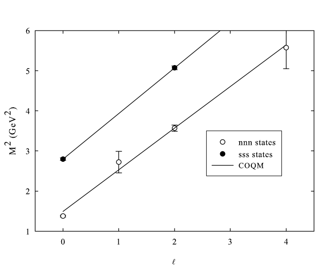
Figure 1: Average experimental square masses of the $nnn$ states (empty circles) and $sss$ states (full circles), compared with the theoretical results (straight lines). The $nnn$ states are computed from the $N$ and $\Delta$ baryons, and the $sss$ states are the $\Omega$ baryons ($W_{nnn}=0.312$ GeV and $W_{sss}=-0.232$ GeV).

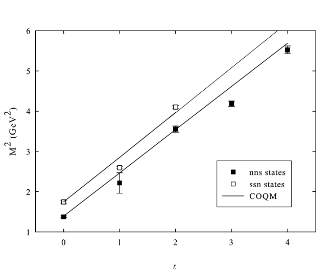
Figure 2: Same as Fig. 1, but for the $nns$ (empty squares) and $ssn$ states (full squares). The $nns$ states are computed from the $\Lambda$ and $\Sigma$ baryons, and the $ssn$ are the $\Xi$ baryons ($W_{nns}=0.379$ GeV and $W_{ssn}=0.223$ GeV).

Like in all potential models, the strength of the confining potential and the constituent quark masses must be fixed on data. We take the spring constants $K_{2}=K_{3}$, as it is argued in Sec. III, and we fix the value of this parameter at $0.107$ GeV³ as in Ref. co93 . The constituent quark masses are chosen to be equal to $m_{n}=0.313$ GeV and $m_{s}=0.375$ GeV, in order to obtain good baryon spectra (these values are different from those used in Ref. co93 ). The results are plotted in Figs. 1 and 2. We can observe a good agreement between the COQM and the average square masses. What is important is that the correct slope is obtained, since the absolute values of the masses depend on ad hoc values of the parameter $W$. $W$ is positive in every case, excepted for the $sss$ baryons. This could be caused by strong spin interactions: masses of the $sss$ states considered are not average ones. Our data concerning the baryons are taken from Ref. pdg .

The difference between the constituent masses $m_{n}$ and $m_{s}$ can seem too small, but such a mass difference is obtained in potential models in which a constituent state dependent mass is defined as $\langle\sqrt{\vec{p}\,^{2}+\nu^{2}}\rangle$ where $\nu$ is the current mass. The value of $m_{s}-m_{n}$ is around 40 MeV in Refs. naro04 ; sema04 for ground states of mesons and baryons. In Ref. kerb00 , an analytical approximate formula is given for the constituent quark mass of the baryon ground states : a difference of about 30 MeV is found for current masses $\nu_{n}=0$ and $\nu_{s}=130$ MeV pdg . In our model, the constituent masses are not state-dependent but, in these references, small values for the difference $m_{s}-m_{n}$ are also found, and absolute masses $m_{n}$ and $m_{s}$ are in agreement with our values.

Formula (6) implies that the square meson masses $M^{2}$ have a linear dependence on the orbital angular momentum $\ell$

$$M^{2}=\beta\ell+\beta_{0}.$$ (41)

This relation is also well verified experimentally. Using the data and the procedure of Ref. Buis05 , average square meson masses can be computed, and the relation (41) can be fitted on these data to obtain an average experimental Regge slope $\beta_{\text{exp.}}$. With our parameters optimized for baryon spectra, a theoretical Regge slope $\beta_{\text{COQM}}$ can be computed for mesons. It can be seen on Table 1 that the two slopes differ only by around 6% for various $q\bar{q}$ systems. By increasing the value of $m_{n}$ by about 30 MeV, it is possible to improve the theoretical meson spectra. The price to pay is a slight deterioration of the baryon spectra.

IV.2 Glueballs

We will assume here that the energy density of the flux tube starting from a particle $i$ is proportional to the Casimir operator $\sum_{b}T^{(i)}_{b}T^{(i)}_{b}$, with $T^{(i)}_{b}$ being a $SU(3)$ generator in the corresponding representation. Several approaches tend to confirm this hypothesis scaling ; new . Then, if $a_{2}$ is the energy density in a meson, we should have $a_{2g}=(9/4)a_{2}$ in a glueball formed of two gluons, and $a_{3g}=a_{2g}$ where $a_{3g}$ is the energy density in a three-gluon glueball. In the COQM, the corresponding spring constants $K_{3g}$ and $K_{2g}$ will thus be given by $K_{3g}=K_{2g}=(9/4)^{2}K_{2}$, where $K_{2}$ is the spring constant for a meson. In order to simulate at best the Y-junction we will also use $\alpha=5/9$ as in the baryonic sector.

The constituent gluon mass $m_{g}$ is a parameter of the model which must be fixed as the constituent quark masses. Because of the scarcity of reliable experimental data, we will determine it by using lattice-QCD results about two-gluon glueball spectrum.. We consider that all the positive charge conjugate states given in Refs. lat99 ; lat05 are two-gluon glueballs. This in agreement with the results of the potential model of Ref. Brau04 . These states are shown in Table 2 with the average square masses computed using Eq. (39). By fitting the mass formula (10) on these data, we obtain $m_{g}=0.770\pm 0.340$ GeV, a value close to the usual ones Brau04 ; new ; abre05 . Formula (10) shows that the two-gluon glueball mass depends on the product $K_{2g}m_{g}$. If we assume a color-dependence on the square-root of the Casimir operator john76 , it is necessary to use a gluon mass around 1.7 GeV, which seems too heavy.

According to the glueball-pomeron theory, the $J^{++}$ two-gluon glueballs, having a maximum intrinsic spin $S$ coupled to a minimum possible orbital angular momentum $\ell$, stand on Regge trajectories. In Ref. donn98 , the following relation is obtained

$$J=0.25\,M^{2}_{gg}+1.08.$$ (42)

This result is close to the one obtained in Ref. meye05 . In Ref. new , the relation obtained is noticeably different

$$J=0.36\,M^{2}_{gg}+{0.80\atop 0.57}.$$ (43)

The value of the ordinate at origin in this model depends on the value chosen for the strong coupling constant. If we use our average square two-gluon glueball masses (see Table 2) and if we assume $J=\ell+2$ (maximum $J$-coupling), we find

$$J=(0.27\pm 0.06)\,M^{2}_{gg}+(0.59\pm 0.49).$$ (44)

One can see that our slope is in agreement with of the slope found in Ref. donn98 , but our ordinate at origin is more compatible with the corresponding one in Ref. new . Finally, Relation (44) is in good agreement with the relation found in the COQM of Ref. co97

$$J=0.26\,M^{2}_{gg}+0.67.$$ (45)

If the interaction between gluons was spin-independent, we could expect that the lightest three-gluon glueballs are the states with a vanishing total orbital angular momentum and $J^{PC}=0^{-+}$, $1^{--}$, $3^{--}$ llan05 . The lattice calculations yield very different results lat99 ; lat05 . This can be due to very large spin-orbit effects, which have been observed in two-gluon glueballs Brau04 . In this situation, we can expect that our spinless COQM can just describe the three-gluon glueballs with a vanishing total orbital angular momentum. An average square mass is obtained in Table 2 with the $1^{--}$, $3^{--}$ states of Ref. lat05 . The $0^{-+}$ state of this work is assumed to be a two-gluon glueball (see above).

The equivalent of the pomeron for three-gluon glueballs is called the odderon. $J^{--}$ three-gluon glueballs, having a maximum intrinsic spin coupled to a minimum possible orbital angular momentum, are also expected to stand on Regge trajectories. The following results are predicted in Ref. llan05 for a QCD effective Hamiltonian and for a non relativistic potential model respectively

$$J_{\text{eff.}} = 0.23\,M^{2}_{ggg}-0.88,$$ (46)

$$J_{\text{NR}} = 0.18\,M^{2}_{ggg}+0.25.$$ (47)

Let us note that a slope for $ggg$ states which is half the slope for $gg$ states has been suggested meye05 .

If we fit our square mass formula (38) with the unique data of Table 2 for three-gluon glueballs, and if we assume $J=\ell+3$ (maximum $J$-coupling) we obtain

$$J=(0.27\pm 0.06)\,M^{2}_{ggg}-(1.57\pm 1.54).$$ (48)

The same slope is predicted for two-gluon and three-gluon glueballs, as in the case of quark systems, because we assume $\alpha=5/9$ and $K_{3g}=K_{2g}$, and also because we choose for the gluon mass the value of 0.770 GeV found for the two-gluon glueballs. Our result is then compatible with the one from the QCD effective Hamiltonian of Ref. llan05 .

It is worth mentioning that the Regge trajectories presented in Refs. donn98 ; new ; llan05 ; meye05 concern glueballs with given $J^{PC}$. Our model can only predict spin average square masses. So, the absolute masses given by our model cannot, in principle, be compared directly with masses of states with given $J^{PC}$. The ordinates at origin of Regge trajectories calculated with our model could then have a significant error, but we can expect a correct computation of the slope.

V Summary of the results

In this paper, we have solved the covariant oscillator quark model applied to three-body systems, with a general quadratic potential. This interaction is a linear combination between a $\Delta$-potential and a simplified Y-junction where the Toricelli point is identified with the center of mass; it is believed to be a good approximation of the true Y-junction potential. We found analytic expressions for the mass spectrum and for the total wave function. We then have shown that our results are in quite good agreement with experimental and lattice data concerning baryons and glueballs provided the Casimir scaling is true. However, a more detailed study of the glueballs with the COQM requires to take into account the spin interactions, which are particularly strong in these particles.

Table 1: Regge slope $\beta$ for mesons (see formula (41)). $\beta_{\text{exp.}}$ is the value obtained by averaging experimental data (see Ref. Buis05 ) and $\beta_{\text{COQM}}$ is our theoretical value (see formula (6)). The values of parameters $W$ for the various systems are also given.

State	$\beta_{\text{exp.}}$ (GeV-2)	$\beta_{\text{COQM}}$ (GeV-2)	$W$ (GeV)
$n\bar{n}$	1.13	1.04	0.370
$n\bar{s}$	1.16	1.09	0.220
$s\bar{s}$	1.19	1.13	0.065

Table 2: Average square masses, $M^{2}_{\text{av}}$, for glueball states. The third and fourth columns show the different states used to compute the quantities $M^{2}_{\text{av}}$. Data are taken from Ref. lat05 , except the mass of the $0^{*}$ state which is taken from Ref. lat99 .

State	$(n+1)L$	$J^{PC}$	$M$ (GeV)	$M^{2}_{\rm{av}}$(GeV2)
$gg$	1S	0++	$1.710\pm 0.130$	$5.183\pm 0.667$
		2++	$2.390\pm 0.150$
	1P	0-+	$2.560\pm 0.155$	$8.762\pm 1.089$
		2-+	$3.040\pm 0.190$
	1D	0∗++	$2.670\pm 0.310$	$12.567\pm 1.702$
		3++	$3.670\pm 0.230$
$ggg$	1S	1–	$3.830\pm 0.230$	$16.720\pm 1.967$
		3–	$4.200\pm 0.245$