Study of Bs→π​ρ→subscriptπ΅π‘ πœ‹πœŒB_{s}\to\pi\rho decays in the perturbative QCD approach

Xian-Qiao Yu111yuxq@mail.ihep.ac.cn, Ying Li222liying@mail.ihep.ac.cn Institute of High Energy Physics, P.O.Box 918(4), Beijing 100049, China; Graduate School of the Chinese Academy of Sciences, Beijing 100049, China    Cai-Dian LΓΌ CCAST (World Laboratory), P.O. Box 8730, Beijing 100080, China; Institute of High Energy Physics, P.O.Box 918(4), Beijing 100049, China333Mailing address
Abstract

In this note, we calculate the branching ratio and $CP$ asymmetry parameters of Bs→π​ρ→subscriptπ΅π‘ πœ‹πœŒB_{s}\rightarrow\pi\rho in the framework of perturbative QCD approach based on $k_{T}$ factorization. This decay can occur only via annihilation diagrams in the Standard Model. We find that (a) the charge averaged $Br(B_{s}\rightarrow\pi^{+}\rho^{-}+\pi^{-}\rho^{+})$ is about $(9-12)\times 10^{-7}$; $Br(B_{s}\rightarrow\pi^{0}\rho^{0})\simeq 4\times 10^{-7}$; and (b) there are sizable $CP$ asymmetries in the processes, which can be tested in the near future Large Hadron Collider beauty experiments (LHC-b) at CERN.

pacs:
13.25.Hw, 12.38.Bx

The $B$ meson rare decays provide a good place for testing the Standard Model (SM), studying $CP$ violation and looking for possible new physics beyond the SM. A lot of theoretical studies have been done in recent years, which are strongly supported by the running $B$ factories in KEK and Stanford Linear Accelerator Center (SLAC). Looking forward to the future CERN Large Hadron Collider beauty experiments (LHC-b), a large number of $B_{s}$ and $B_{c}$ mesons can also be produced. So the studies of $B_{s}$ meson rare decays are necessary in the next a few years.

In this paper, we study the rare decays Bs→π​ρ→subscriptπ΅π‘ πœ‹πœŒB_{s}\to\pi\rho in Perturbative QCD approach (PQCD) LY . Comparing with QCD factorization approach bbns , PQCD approach can make a reliable calculation for pure annihilation diagrams in $k_{T}$ factorization. The endpoint singularity occurred in QCD factorization approach can be cured here by the Sudakov factor from resummation of double logarithms.

In PQCD approach, the decay amplitude can be written as:

$$\mbox{Amplitude}\sim\int\!\!d^{4}k_{1}d^{4}k_{2}d^{4}k_{3}\ \mathrm{Tr}\bigl{[}C(t)\Phi_{B_{s}}(k_{1})\Phi_{\pi}(k_{2})\Phi_{\rho}(k_{3})H(k_{1},k_{2},k_{3},t)\bigr{]}e^{-S(t)}.$$ (1)

In our following calculations, the Wilson coefficient $C(t)$, Sudakov factor Si​(t)​(i=Bs,Ο€,ρ)subscript𝑆𝑖𝑑𝑖subscriptπ΅π‘ πœ‹πœŒS_{i}(t)(i=B_{s},\pi,\rho) and the non-perturbative but universal wave function $\Phi_{i}$ can be found in the Refs. LUY ; YLL ; BFB ; BBKT ; LYE . The hard part $H$ are channel dependent but fortunately perturbative calculable, which will be shown below.

Refer to caption
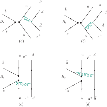
Figure 1: The lowest order diagrams for $B_{s}\rightarrow\pi^{+}\rho^{-}$ decay

Like the $B_{s}\rightarrow\pi^{+}\pi^{-}$ decay LLXY , the Bs→π​ρ→subscriptπ΅π‘ πœ‹πœŒB_{s}\rightarrow\pi\rho decays are pure annihilation type rare decays, which are difficult to be calculated in method other than PQCD approach. Fig.Β 1 shows the lowest order Feynman diagrams to be calculated in PQCD approach where the big dots denote the quark currents in four quark operators for $B_{s}\rightarrow\pi^{+}\rho^{-}$ according to the effective hamiltonian of $b$ quark decay BBL . First for the usual factorizable diagram (a) and (b), the sum of (V-A)(V-A) current contributions is given by

Ma[C]=16Ο€CFMB2∫01dx2dx3∫0∞b2db2b3db3{[x3ϕπA(x2)ϕρ(x3)+2rΟ€rρ(1+x3)ϕπP(x2)ϕρs(x3)+2rΟ€rρ(x3βˆ’1)ϕπP(x2)ϕρt(x3)]Ξ±s(ta1)ha(x2,x3,b2,b3)exp[βˆ’SΟ€(ta1)βˆ’Sρ(ta1)]C(ta1)βˆ’[x2​ϕπA​(x2)​ϕρ​(x3)+2​rπ​rρ​(1+x2)​ϕπP​(x2)​ϕρs​(x3)+2​rπ​rρ​(x2βˆ’1)​ϕπT​(x2)​ϕρs​(x3)]Ξ±s(ta2)ha(x3,x2,b3,b2)exp[βˆ’SΟ€(ta2)βˆ’Sρ(ta2)]C(ta2)},subscriptπ‘€π‘Ždelimited-[]𝐢16πœ‹subscript𝐢𝐹superscriptsubscript𝑀𝐡2superscriptsubscript01𝑑subscriptπ‘₯2𝑑subscriptπ‘₯3superscriptsubscript0subscript𝑏2𝑑subscript𝑏2subscript𝑏3𝑑subscript𝑏3delimited-[]subscriptπ‘₯3superscriptsubscriptitalic-Ο•πœ‹π΄subscriptπ‘₯2subscriptitalic-Ο•πœŒsubscriptπ‘₯32subscriptπ‘Ÿπœ‹subscriptπ‘ŸπœŒ1subscriptπ‘₯3superscriptsubscriptitalic-Ο•πœ‹π‘ƒsubscriptπ‘₯2superscriptsubscriptitalic-Ο•πœŒπ‘ subscriptπ‘₯32subscriptπ‘Ÿπœ‹subscriptπ‘ŸπœŒsubscriptπ‘₯31superscriptsubscriptitalic-Ο•πœ‹π‘ƒsubscriptπ‘₯2superscriptsubscriptitalic-Ο•πœŒπ‘‘subscriptπ‘₯3subscript𝛼𝑠superscriptsubscriptπ‘‘π‘Ž1subscriptβ„Žπ‘Žsubscriptπ‘₯2subscriptπ‘₯3subscript𝑏2subscript𝑏3subscriptπ‘†πœ‹superscriptsubscriptπ‘‘π‘Ž1subscriptπ‘†πœŒsuperscriptsubscriptπ‘‘π‘Ž1𝐢superscriptsubscriptπ‘‘π‘Ž1delimited-[]subscriptπ‘₯2superscriptsubscriptitalic-Ο•πœ‹π΄subscriptπ‘₯2subscriptitalic-Ο•πœŒsubscriptπ‘₯32subscriptπ‘Ÿπœ‹subscriptπ‘ŸπœŒ1subscriptπ‘₯2superscriptsubscriptitalic-Ο•πœ‹π‘ƒsubscriptπ‘₯2superscriptsubscriptitalic-Ο•πœŒπ‘ subscriptπ‘₯32subscriptπ‘Ÿπœ‹subscriptπ‘ŸπœŒsubscriptπ‘₯21superscriptsubscriptitalic-Ο•πœ‹π‘‡subscriptπ‘₯2superscriptsubscriptitalic-Ο•πœŒπ‘ subscriptπ‘₯3subscript𝛼𝑠superscriptsubscriptπ‘‘π‘Ž2subscriptβ„Žπ‘Žsubscriptπ‘₯3subscriptπ‘₯2subscript𝑏3subscript𝑏2subscriptπ‘†πœ‹superscriptsubscriptπ‘‘π‘Ž2subscriptπ‘†πœŒsuperscriptsubscriptπ‘‘π‘Ž2𝐢superscriptsubscriptπ‘‘π‘Ž2M_{a}[C]=16\pi C_{F}M_{B}^{2}\int_{0}^{1}\!\!\!dx_{2}dx_{3}\int_{0}^{\infty}\!\!\!\!\!b_{2}db_{2}\,b_{3}db_{3}\ \bigl{\{}[x_{3}\phi_{\pi}^{A}(x_{2})\phi_{\rho}(x_{3})+2r_{\pi}r_{\rho}(1+x_{3})\phi_{\pi}^{P}(x_{2})\phi_{\rho}^{s}(x_{3})\\ +2r_{\pi}r_{\rho}(x_{3}-1)\phi_{\pi}^{P}(x_{2})\phi_{\rho}^{t}(x_{3})]\alpha_{s}(t_{a}^{1})h_{a}(x_{2},x_{3},b_{2},b_{3})\exp[-S_{\pi}(t_{a}^{1})-S_{\rho}(t_{a}^{1})]C(t_{a}^{1})\\ -[x_{2}\phi_{\pi}^{A}(x_{2})\phi_{\rho}(x_{3})+2r_{\pi}r_{\rho}(1+x_{2})\phi_{\pi}^{P}(x_{2})\phi_{\rho}^{s}(x_{3})+2r_{\pi}r_{\rho}(x_{2}-1)\phi_{\pi}^{T}(x_{2})\phi_{\rho}^{s}(x_{3})]\\ \alpha_{s}(t_{a}^{2})h_{a}(x_{3},x_{2},b_{3},b_{2})\exp[-S_{\pi}(t_{a}^{2})-S_{\rho}(t_{a}^{2})]C(t_{a}^{2})\bigr{\}}, (2)

where $r_{\pi}=m_{0\pi}/m_{B}=m_{\pi}^{2}/[m_{B}(m_{u}+m_{d})]$, $r_{\rho}=m_{\rho}/m_{B}$. $C_{F}=4/3$ is the group factor of the $SU(3)_{c}$ gauge group. $\phi_{i}$ is light cone distribution amplitude, which describes the momentum distribution of the meson wave function. The function

$\displaystyle h_{a}(x_{2},x_{3},b_{2},b_{3})=S_{t}(x_{3})\frac{\pi i}{2}H_{0}^{(1)}(M_{B}\sqrt{x_{2}x_{3}}b_{2})$
$\displaystyle\times\bigl{[}\theta(b_{2}-b_{3})J_{0}(M_{B}\sqrt{x_{3}}b_{3})\frac{\pi i}{2}H_{0}^{(1)}(M_{B}\sqrt{x_{3}}b_{2})+(b_{2}\leftrightarrow b_{3})\bigr{]}$ (3)

comes from the Fourier transformation of propagators of virtual quark and gluon in the hard part calculations. $S_{t}(x)$ results from the threshold resummation of QCD radiative corrections to hard amplitudes KLS . $H_{0}^{1}(z)=J_{0}(z)+iY_{0}(z)$, $J_{0}$ and $Y_{0}$ are Bessel functions. The sum of (V-A)(V+A) current contributions of diagrams (a) and (b) is $-M_{a}[C]$.

For the non-factorizable annihilation diagrams (c) and (d), all three meson wave functions are involved. The (V-A)(V-A) operator’s contribution is:

Mc​[C]=βˆ’12​Nc​64​π​CF​MB2β€‹βˆ«01𝑑x1​𝑑x2​𝑑x3β€‹βˆ«0∞b1​𝑑b1​b2​𝑑b2​ϕB​(x1,b1)Γ—{[βˆ’x2ϕρ(x3)ϕπA(x2)+rρrΟ€(x3βˆ’x2)ϕρt(x3)ϕπP(x2)βˆ’rρrΟ€(x2+x3)ϕρs(x3)ϕπP(x2)βˆ’rΟ€rρ(x2+x3)ϕρt(x3)ϕπT(x2)+rΟ€rρ(x3βˆ’x2)ϕρs(x3)ϕπT(x2)]C(tc1)Ξ±s(tc1)hc(1)(x1,x2,x3,b1,b2)exp[βˆ’SB(tc1)βˆ’SΟ€(tc1)βˆ’Sρ(tc1)]βˆ’[βˆ’x3ϕρ(x3)ϕπA(x2)+rρ​rπ​(x2βˆ’x3)​ϕρt​(x3)​ϕπP​(x2)βˆ’rρ​rπ​(2+x2+x3)​ϕρs​(x3)​ϕπP​(x2)+rΟ€rρ(2βˆ’x2βˆ’x3)ϕρt(x3)ϕπT(x2)+rΟ€rρ(x2βˆ’x3)ϕρs(x3)ϕπT(x2)]C(tc2)Ξ±s(tc2)hc(2)(x1,x2,x3,b1,b2)exp[βˆ’SB(tc2)βˆ’SΟ€(tc2)βˆ’Sρ(tc2)]}.subscript𝑀𝑐delimited-[]𝐢12subscript𝑁𝑐64πœ‹subscript𝐢𝐹superscriptsubscript𝑀𝐡2superscriptsubscript01differential-dsubscriptπ‘₯1differential-dsubscriptπ‘₯2differential-dsubscriptπ‘₯3superscriptsubscript0subscript𝑏1differential-dsubscript𝑏1subscript𝑏2differential-dsubscript𝑏2subscriptitalic-ϕ𝐡subscriptπ‘₯1subscript𝑏1delimited-[]subscriptπ‘₯2subscriptitalic-Ο•πœŒsubscriptπ‘₯3superscriptsubscriptitalic-Ο•πœ‹π΄subscriptπ‘₯2subscriptπ‘ŸπœŒsubscriptπ‘Ÿπœ‹subscriptπ‘₯3subscriptπ‘₯2superscriptsubscriptitalic-Ο•πœŒπ‘‘subscriptπ‘₯3superscriptsubscriptitalic-Ο•πœ‹π‘ƒsubscriptπ‘₯2subscriptπ‘ŸπœŒsubscriptπ‘Ÿπœ‹subscriptπ‘₯2subscriptπ‘₯3superscriptsubscriptitalic-Ο•πœŒπ‘ subscriptπ‘₯3superscriptsubscriptitalic-Ο•πœ‹π‘ƒsubscriptπ‘₯2subscriptπ‘Ÿπœ‹subscriptπ‘ŸπœŒsubscriptπ‘₯2subscriptπ‘₯3superscriptsubscriptitalic-Ο•πœŒπ‘‘subscriptπ‘₯3superscriptsubscriptitalic-Ο•πœ‹π‘‡subscriptπ‘₯2subscriptπ‘Ÿπœ‹subscriptπ‘ŸπœŒsubscriptπ‘₯3subscriptπ‘₯2superscriptsubscriptitalic-Ο•πœŒπ‘ subscriptπ‘₯3superscriptsubscriptitalic-Ο•πœ‹π‘‡subscriptπ‘₯2𝐢superscriptsubscript𝑑𝑐1subscript𝛼𝑠superscriptsubscript𝑑𝑐1superscriptsubscriptβ„Žπ‘1subscriptπ‘₯1subscriptπ‘₯2subscriptπ‘₯3subscript𝑏1subscript𝑏2subscript𝑆𝐡superscriptsubscript𝑑𝑐1subscriptπ‘†πœ‹superscriptsubscript𝑑𝑐1subscriptπ‘†πœŒsuperscriptsubscript𝑑𝑐1delimited-[]subscriptπ‘₯3subscriptitalic-Ο•πœŒsubscriptπ‘₯3superscriptsubscriptitalic-Ο•πœ‹π΄subscriptπ‘₯2subscriptπ‘ŸπœŒsubscriptπ‘Ÿπœ‹subscriptπ‘₯2subscriptπ‘₯3superscriptsubscriptitalic-Ο•πœŒπ‘‘subscriptπ‘₯3superscriptsubscriptitalic-Ο•πœ‹π‘ƒsubscriptπ‘₯2subscriptπ‘ŸπœŒsubscriptπ‘Ÿπœ‹2subscriptπ‘₯2subscriptπ‘₯3superscriptsubscriptitalic-Ο•πœŒπ‘ subscriptπ‘₯3superscriptsubscriptitalic-Ο•πœ‹π‘ƒsubscriptπ‘₯2subscriptπ‘Ÿπœ‹subscriptπ‘ŸπœŒ2subscriptπ‘₯2subscriptπ‘₯3superscriptsubscriptitalic-Ο•πœŒπ‘‘subscriptπ‘₯3superscriptsubscriptitalic-Ο•πœ‹π‘‡subscriptπ‘₯2subscriptπ‘Ÿπœ‹subscriptπ‘ŸπœŒsubscriptπ‘₯2subscriptπ‘₯3superscriptsubscriptitalic-Ο•πœŒπ‘ subscriptπ‘₯3superscriptsubscriptitalic-Ο•πœ‹π‘‡subscriptπ‘₯2𝐢superscriptsubscript𝑑𝑐2subscript𝛼𝑠superscriptsubscript𝑑𝑐2superscriptsubscriptβ„Žπ‘2subscriptπ‘₯1subscriptπ‘₯2subscriptπ‘₯3subscript𝑏1subscript𝑏2subscript𝑆𝐡superscriptsubscript𝑑𝑐2subscriptπ‘†πœ‹superscriptsubscript𝑑𝑐2subscriptπ‘†πœŒsuperscriptsubscript𝑑𝑐2M_{c}[C]=\frac{-1}{\sqrt{2N_{c}}}64\pi C_{F}M_{B}^{2}\int_{0}^{1}\!\!\!dx_{1}dx_{2}dx_{3}\int_{0}^{\infty}\!\!\!\!\!b_{1}db_{1}\ b_{2}db_{2}\ \phi_{B}(x_{1},b_{1})\\ \times\bigl{\{}[-x_{2}\phi_{\rho}(x_{3})\phi_{\pi}^{A}(x_{2})+r_{\rho}r_{\pi}(x_{3}-x_{2})\phi_{\rho}^{t}(x_{3})\phi_{\pi}^{P}(x_{2})-r_{\rho}r_{\pi}(x_{2}+x_{3})\phi_{\rho}^{s}(x_{3})\phi_{\pi}^{P}(x_{2})\\ -r_{\pi}r_{\rho}(x_{2}+x_{3})\phi_{\rho}^{t}(x_{3})\phi_{\pi}^{T}(x_{2})+r_{\pi}r_{\rho}(x_{3}-x_{2})\phi_{\rho}^{s}(x_{3})\phi_{\pi}^{T}(x_{2})]\\ C(t_{c}^{1})\alpha_{s}(t_{c}^{1})h_{c}^{(1)}(x_{1},x_{2},x_{3},b_{1},b_{2})\exp[-S_{B}(t_{c}^{1})-S_{\pi}(t_{c}^{1})-S_{\rho}(t_{c}^{1})]-[-x_{3}\phi_{\rho}(x_{3})\phi_{\pi}^{A}(x_{2})\\ +r_{\rho}r_{\pi}(x_{2}-x_{3})\phi_{\rho}^{t}(x_{3})\phi_{\pi}^{P}(x_{2})-r_{\rho}r_{\pi}(2+x_{2}+x_{3})\phi_{\rho}^{s}(x_{3})\phi_{\pi}^{P}(x_{2})\\ +r_{\pi}r_{\rho}(2-x_{2}-x_{3})\phi_{\rho}^{t}(x_{3})\phi_{\pi}^{T}(x_{2})+r_{\pi}r_{\rho}(x_{2}-x_{3})\phi_{\rho}^{s}(x_{3})\phi_{\pi}^{T}(x_{2})]\\ C(t_{c}^{2})\alpha_{s}(t_{c}^{2})h_{c}^{(2)}(x_{1},x_{2},x_{3},b_{1},b_{2})\exp[-S_{B}(t_{c}^{2})-S_{\pi}(t_{c}^{2})-S_{\rho}(t_{c}^{2})]\bigr{\}}. (4)

For the penguin operators, there are also $(V-A)(V+A)$ type operators, whose contribution is given as

McP​[C]=12​Nc​64​π​CF​MB2β€‹βˆ«01𝑑x1​𝑑x2​𝑑x3β€‹βˆ«0∞b1​𝑑b1​b2​𝑑b2​ϕB​(x1,b1)Γ—{[βˆ’x3ϕρ(x3)ϕπA(x2)βˆ’rρrΟ€(x3βˆ’x2)ϕρt(x3)ϕπP(x2)βˆ’rρrΟ€(x2+x3)ϕρs(x3)ϕπP(x2)βˆ’rΟ€rρ(x2+x3)ϕρt(x3)ϕπT(x2)βˆ’rΟ€rρ(x3βˆ’x2)ϕρs(x3)ϕπT(x2)]C(tc1)Ξ±s(tc1)hc(1)(x1,x2,x3,b1,b2)exp[βˆ’SB(tc1)βˆ’SΟ€(tc1)βˆ’Sρ(tc1)]βˆ’[βˆ’x2ϕρ(x3)ϕπA(x2)βˆ’rρ​rπ​(x2βˆ’x3)​ϕρt​(x3)​ϕπP​(x2)βˆ’rρ​rπ​(2+x2+x3)​ϕρs​(x3)​ϕπP​(x2)+rΟ€rρ(2βˆ’x2βˆ’x3)ϕρt(x3)ϕπT(x2)βˆ’rΟ€rρ(x2βˆ’x3)ϕρs(x3)ϕπT(x2)]C(tc2)Ξ±s(tc2)hc(2)(x1,x2,x3,b1,b2)exp[βˆ’SB(tc2)βˆ’SΟ€(tc2)βˆ’Sρ(tc2)]},superscriptsubscript𝑀𝑐𝑃delimited-[]𝐢12subscript𝑁𝑐64πœ‹subscript𝐢𝐹superscriptsubscript𝑀𝐡2superscriptsubscript01differential-dsubscriptπ‘₯1differential-dsubscriptπ‘₯2differential-dsubscriptπ‘₯3superscriptsubscript0subscript𝑏1differential-dsubscript𝑏1subscript𝑏2differential-dsubscript𝑏2subscriptitalic-ϕ𝐡subscriptπ‘₯1subscript𝑏1delimited-[]subscriptπ‘₯3subscriptitalic-Ο•πœŒsubscriptπ‘₯3superscriptsubscriptitalic-Ο•πœ‹π΄subscriptπ‘₯2subscriptπ‘ŸπœŒsubscriptπ‘Ÿπœ‹subscriptπ‘₯3subscriptπ‘₯2superscriptsubscriptitalic-Ο•πœŒπ‘‘subscriptπ‘₯3superscriptsubscriptitalic-Ο•πœ‹π‘ƒsubscriptπ‘₯2subscriptπ‘ŸπœŒsubscriptπ‘Ÿπœ‹subscriptπ‘₯2subscriptπ‘₯3superscriptsubscriptitalic-Ο•πœŒπ‘ subscriptπ‘₯3superscriptsubscriptitalic-Ο•πœ‹π‘ƒsubscriptπ‘₯2subscriptπ‘Ÿπœ‹subscriptπ‘ŸπœŒsubscriptπ‘₯2subscriptπ‘₯3superscriptsubscriptitalic-Ο•πœŒπ‘‘subscriptπ‘₯3superscriptsubscriptitalic-Ο•πœ‹π‘‡subscriptπ‘₯2subscriptπ‘Ÿπœ‹subscriptπ‘ŸπœŒsubscriptπ‘₯3subscriptπ‘₯2superscriptsubscriptitalic-Ο•πœŒπ‘ subscriptπ‘₯3superscriptsubscriptitalic-Ο•πœ‹π‘‡subscriptπ‘₯2𝐢superscriptsubscript𝑑𝑐1subscript𝛼𝑠superscriptsubscript𝑑𝑐1superscriptsubscriptβ„Žπ‘1subscriptπ‘₯1subscriptπ‘₯2subscriptπ‘₯3subscript𝑏1subscript𝑏2subscript𝑆𝐡superscriptsubscript𝑑𝑐1subscriptπ‘†πœ‹superscriptsubscript𝑑𝑐1subscriptπ‘†πœŒsuperscriptsubscript𝑑𝑐1delimited-[]subscriptπ‘₯2subscriptitalic-Ο•πœŒsubscriptπ‘₯3superscriptsubscriptitalic-Ο•πœ‹π΄subscriptπ‘₯2subscriptπ‘ŸπœŒsubscriptπ‘Ÿπœ‹subscriptπ‘₯2subscriptπ‘₯3superscriptsubscriptitalic-Ο•πœŒπ‘‘subscriptπ‘₯3superscriptsubscriptitalic-Ο•πœ‹π‘ƒsubscriptπ‘₯2subscriptπ‘ŸπœŒsubscriptπ‘Ÿπœ‹2subscriptπ‘₯2subscriptπ‘₯3superscriptsubscriptitalic-Ο•πœŒπ‘ subscriptπ‘₯3superscriptsubscriptitalic-Ο•πœ‹π‘ƒsubscriptπ‘₯2subscriptπ‘Ÿπœ‹subscriptπ‘ŸπœŒ2subscriptπ‘₯2subscriptπ‘₯3superscriptsubscriptitalic-Ο•πœŒπ‘‘subscriptπ‘₯3superscriptsubscriptitalic-Ο•πœ‹π‘‡subscriptπ‘₯2subscriptπ‘Ÿπœ‹subscriptπ‘ŸπœŒsubscriptπ‘₯2subscriptπ‘₯3superscriptsubscriptitalic-Ο•πœŒπ‘ subscriptπ‘₯3superscriptsubscriptitalic-Ο•πœ‹π‘‡subscriptπ‘₯2𝐢superscriptsubscript𝑑𝑐2subscript𝛼𝑠superscriptsubscript𝑑𝑐2superscriptsubscriptβ„Žπ‘2subscriptπ‘₯1subscriptπ‘₯2subscriptπ‘₯3subscript𝑏1subscript𝑏2subscript𝑆𝐡superscriptsubscript𝑑𝑐2subscriptπ‘†πœ‹superscriptsubscript𝑑𝑐2subscriptπ‘†πœŒsuperscriptsubscript𝑑𝑐2M_{c}^{P}[C]=\frac{1}{\sqrt{2N_{c}}}64\pi C_{F}M_{B}^{2}\int_{0}^{1}\!\!\!dx_{1}dx_{2}dx_{3}\int_{0}^{\infty}\!\!\!\!\!b_{1}db_{1}\ b_{2}db_{2}\ \phi_{B}(x_{1},b_{1})\\ \times\bigl{\{}[-x_{3}\phi_{\rho}(x_{3})\phi_{\pi}^{A}(x_{2})-r_{\rho}r_{\pi}(x_{3}-x_{2})\phi_{\rho}^{t}(x_{3})\phi_{\pi}^{P}(x_{2})-r_{\rho}r_{\pi}(x_{2}+x_{3})\phi_{\rho}^{s}(x_{3})\phi_{\pi}^{P}(x_{2})\\ -r_{\pi}r_{\rho}(x_{2}+x_{3})\phi_{\rho}^{t}(x_{3})\phi_{\pi}^{T}(x_{2})-r_{\pi}r_{\rho}(x_{3}-x_{2})\phi_{\rho}^{s}(x_{3})\phi_{\pi}^{T}(x_{2})]\\ C(t_{c}^{1})\alpha_{s}(t_{c}^{1})h_{c}^{(1)}(x_{1},x_{2},x_{3},b_{1},b_{2})\exp[-S_{B}(t_{c}^{1})-S_{\pi}(t_{c}^{1})-S_{\rho}(t_{c}^{1})]-[-x_{2}\phi_{\rho}(x_{3})\phi_{\pi}^{A}(x_{2})\\ -r_{\rho}r_{\pi}(x_{2}-x_{3})\phi_{\rho}^{t}(x_{3})\phi_{\pi}^{P}(x_{2})-r_{\rho}r_{\pi}(2+x_{2}+x_{3})\phi_{\rho}^{s}(x_{3})\phi_{\pi}^{P}(x_{2})\\ +r_{\pi}r_{\rho}(2-x_{2}-x_{3})\phi_{\rho}^{t}(x_{3})\phi_{\pi}^{T}(x_{2})-r_{\pi}r_{\rho}(x_{2}-x_{3})\phi_{\rho}^{s}(x_{3})\phi_{\pi}^{T}(x_{2})]\\ C(t_{c}^{2})\alpha_{s}(t_{c}^{2})h_{c}^{(2)}(x_{1},x_{2},x_{3},b_{1},b_{2})\exp[-S_{B}(t_{c}^{2})-S_{\pi}(t_{c}^{2})-S_{\rho}(t_{c}^{2})]\bigr{\}}, (5)

where

$\displaystyle h^{(j)}_{c}(x_{1},x_{2},x_{3},b_{1},b_{2})=$
$\displaystyle\biggl{\{}\theta(b_{2}-b_{1})\frac{\pi i}{2}\mathrm{H}_{0}^{(1)}(M_{B}\sqrt{x_{2}x_{3}}\,b_{2})\mathrm{J}_{0}(M_{B}\sqrt{x_{2}x_{3}}\,b_{1})$
$\displaystyle\qquad\qquad\qquad\qquad+(b_{1}\leftrightarrow b_{2})\biggr{\}}\times\left(\begin{matrix}\mathrm{K}_{0}(M_{B}F_{(j)}b_{1}),&\text{for}\quad F^{2}_{(j)}>0\\ \frac{\pi i}{2}\mathrm{H}_{0}^{(1)}(M_{B}\sqrt{|F^{2}_{(j)}|}\ b_{1}),&\text{for}\quad F^{2}_{(j)}<0\end{matrix}\right),$ (6)

$K_{0}$ is modified Bessel function and $F_{(j)}$’s are defined by

$$F^{2}_{(1)}=x_{1}x_{2}-x_{2}x_{3};\ F^{2}_{(2)}=x_{1}+x_{2}+x_{3}-x_{1}x_{2}-x_{2}x_{3}.$$ (7)

The hard scale $t_{i}^{\prime}s$ in Eqs.(2, 4, 5) are chosen as the largest energy scale appearing in each diagram to kill the large logarithmic corrections:

$\displaystyle t_{a}^{1}$ $\displaystyle=$ $\displaystyle\mathrm{max}(M_{B}\sqrt{x_{3}},1/b_{2},1/b_{3}),$
$\displaystyle t_{a}^{2}$ $\displaystyle=$ $\displaystyle\mathrm{max}(M_{B}\sqrt{x_{2}},1/b_{2},1/b_{3}),$
$\displaystyle t_{c}^{1}$ $\displaystyle=$ $\displaystyle\mathrm{max}(M_{B}\sqrt{|F^{2}_{(1)}|},M_{B}\sqrt{x_{2}x_{3}},1/b_{1},1/b_{2}),$
$\displaystyle t_{c}^{2}$ $\displaystyle=$ $\displaystyle\mathrm{max}(M_{B}\sqrt{|F^{2}_{(2)}|},M_{B}\sqrt{x_{2}x_{3}},1/b_{1},1/b_{2}).$

The total decay amplitude is then

$\displaystyle{\cal A}(B_{s}\to\pi^{+}\rho^{-})=f_{B}M_{a}\left[V_{ub}^{*}V_{us}(C_{1}+\frac{1}{3}C_{2})-V_{tb}^{*}V_{ts}(2C_{3}+\frac{2}{3}C_{4}-2C_{5}-\frac{2}{3}C_{6}-\frac{1}{2}C_{7}-\frac{1}{6}C_{8}+\frac{1}{2}C_{9}+\frac{1}{6}C_{10})\right]$
$\displaystyle+M_{c}\left[V_{ub}^{*}V_{us}C_{2}-V_{tb}^{*}V_{ts}(2C_{4}+\frac{1}{2}C_{10})\right]-V_{tb}^{*}V_{ts}M_{c}^{P}\left(2C_{6}+\frac{1}{2}C_{8}\right),\hskip 142.26378pt.$ (8)

and the decay width is expressed as

$$\Gamma(B_{s}\to\pi^{+}\rho^{-})=\frac{G_{F}^{2}M_{B}^{3}}{128\pi}\left|{\cal A}(B_{s}\rightarrow\pi^{+}\rho^{-})\right|^{2}.$$ (9)

The most important contribution here is the factorizable penguin diagram, which is CKM enhanced. If we exchange the $\pi$ and $\rho$ in Fig. 1, by the same method, we can compute the $B_{s}\rightarrow\pi^{-}\rho^{+}$ decay. The expressions are similar. The decay amplitude for $B_{s}\to\pi^{0}\rho^{0}$ is

$${\cal A}(B_{s}\to\pi^{0}\rho^{0})={\cal A}(B_{s}\to\pi^{+}\rho^{-})+{\cal A}(B_{s}\to\pi^{-}\rho^{+}),$$ (10)

and the decay width can be written as

$$\Gamma(B_{s}\to\pi^{0}\rho^{0})=\frac{G_{F}^{2}M_{B}^{3}}{512\pi}\left|{\cal A}(B_{s}\to\pi^{0}\rho^{0})\right|^{2}.$$ (11)

In the following, we first give the branching ratios of Bs→π​ρ→subscriptπ΅π‘ πœ‹πœŒB_{s}\rightarrow\pi\rho. Just as in Ref. LLXY , we leave the CKM angle $\gamma$ as a free parameter in our numerical calculations. Because there are four decay channels: $B_{s}/\bar{B}_{s}\rightarrow\pi^{+}\rho^{-}$, $B_{s}/\bar{B}_{s}\rightarrow\pi^{-}\rho^{+}$, it is not possible to distinguish the initial state by detecting the final states. We average the sum of $B_{s}/\bar{B}_{s}\rightarrow\pi^{+}\rho^{-}$ as one channel, and $B_{s}/\bar{B}_{s}\rightarrow\pi^{-}\rho^{+}$ as another, which is distinguishable by experiments. Using the same parameters as refs. YLL ; LYE , we get

$\displaystyle\mathbf{Br}(B_{s}/\bar{B}_{s}\rightarrow\pi^{+}\rho^{-})=(5.1^{+0.8}_{-0.5})\times 10^{-7},$
$\displaystyle\mathbf{Br}(B_{s}/\bar{B}_{s}\rightarrow\pi^{-}\rho^{+})=(5.4^{+0.5}_{-0.8})\times 10^{-7},$
$\displaystyle\mathbf{Br}(B_{s}/\bar{B}_{s}\rightarrow\pi^{0}\rho^{0})=(4.2^{+0.6}_{-0.7})\times 10^{-7},$ (12)

where all channels are averaged for $B_{s}$ and $\bar{B}_{s}$.

In Ref. BN , Beneke $et\,al$ have estimated the branching ratio of $\bar{B}_{s}\rightarrow\pi^{+}\rho^{-}$ in the QCD factorization approach. Weak annihilation diagrams are power suppressed in the heavy quark limit and, in general, not calculable in QCD factorization approach. In order to avoid the end-poind singularities, they introduced phenomenological parameters to replace the divergent integral. With those parameters they estimated that the branching ratio of $\bar{B}_{s}\rightarrow\pi^{+}\rho^{-}$ is $(0.03-0.14)\times 10^{-7}$. In PQCD approach, the annihilation amplitude is calculable. In the rest frame of the $B_{s}$ meson, the d or $\bar{d}$ quark included in $\rho$ or $\pi$ has momentum ${\cal O}(M_{B}/4)$, and the gluon producing them has momentum $q^{2}={\cal O}(M_{B}^{2}/4)$. This is a hard gluon, the PQCD can be safely used because of asymptotic freedom of QCD GWP . We have tested that the bulk of the result comes from the region with Ξ±s/Ο€<0.2subscriptπ›Όπ‘ πœ‹0.2\alpha_{s}/\pi<0.2, where a figure was show in Ref. LLX . Our predicted result is larger than their estimation, which can be tested by the future experiments.

Using the same definition in Ref.Β LLXY , we study the $CP$ violation parameters $A^{dir}_{CP}$ and $a_{\epsilon+\epsilon^{{}^{\prime}}}$ in the process of $B_{s}\rightarrow\pi^{0}\rho^{0}$ decay. We find the direct $CP$ violation parameter $A^{dir}_{CP}(B_{s}\rightarrow\pi^{0}\rho^{0})$ is about $2\%$ when $\gamma$ is near $100^{\circ}$, the small direct $CP$ asymmetry is also a result of small tree level contribution. The mixing $CP$ violation parameter $a_{\epsilon+\epsilon^{{}^{\prime}}}(B_{s}\rightarrow\pi^{0}\rho^{0})$ is large, whose peak is close to $16\%$ (see Fig.Β 2).

Refer to caption
Figure 2: Mixing $CP$ violation parameter of $B_{s}\to\pi^{0}\rho^{0}$ decay as a function of CKM angle $\gamma$

The $CP$ violations of $B_{s}/\bar{B}_{s}\rightarrow\pi^{\pm}\rho^{\mp}$ are very complicated. There are four decay amplitudes, which can be expressed as:

g=βŸ¨Ο€+β€‹Οβˆ’|He​f​f|Bs⟩;h=βŸ¨Ο€+β€‹Οβˆ’|He​f​f|BΒ―s⟩;formulae-sequence𝑔quantum-operator-productsuperscriptπœ‹superscript𝜌subscript𝐻𝑒𝑓𝑓subscriptπ΅π‘ β„Žquantum-operator-productsuperscriptπœ‹superscript𝜌subscript𝐻𝑒𝑓𝑓subscript¯𝐡𝑠\displaystyle g=\langle\pi^{+}\rho^{-}|H_{eff}|B_{s}\rangle;\hskip 28.45274pth=\langle\pi^{+}\rho^{-}|H_{eff}|\bar{B}_{s}\rangle;
gΒ―=βŸ¨Ο€βˆ’β€‹Ο+|He​f​f|BΒ―s⟩;hΒ―=βŸ¨Ο€βˆ’β€‹Ο+|He​f​f|Bs⟩.formulae-sequence¯𝑔quantum-operator-productsuperscriptπœ‹superscript𝜌subscript𝐻𝑒𝑓𝑓subscriptΒ―π΅π‘ Β―β„Žquantum-operator-productsuperscriptπœ‹superscript𝜌subscript𝐻𝑒𝑓𝑓subscript𝐡𝑠\displaystyle\bar{g}=\langle\pi^{-}\rho^{+}|H_{eff}|\bar{B}_{s}\rangle;\hskip 28.45274pt\bar{h}=\langle\pi^{-}\rho^{+}|H_{eff}|B_{s}\rangle. (13)

We introduce four parameters to describe the $CP$ asymmetries in the processes, which are given by G

$\displaystyle C_{\pi\rho}=\frac{1}{2}(a_{\epsilon^{{}^{\prime}}}+a_{\bar{\epsilon}^{{}^{\prime}}}),\hskip 42.67912pt\Delta C_{\pi\rho}=\frac{1}{2}(a_{\epsilon^{{}^{\prime}}}-a_{\bar{\epsilon}^{{}^{\prime}}}),$
$\displaystyle S_{\pi\rho}=\frac{1}{2}(a_{\epsilon+\epsilon^{{}^{\prime}}}+a_{\epsilon+\bar{\epsilon}^{{}^{\prime}}}),\hskip 28.45274pt\Delta S_{\pi\rho}=\frac{1}{2}(a_{\epsilon+\epsilon^{{}^{\prime}}}-a_{\epsilon+\bar{\epsilon}^{{}^{\prime}}}),$ (14)

where

$\displaystyle a_{\epsilon^{{}^{\prime}}}=\frac{|g|^{2}-|h|^{2}}{|g|^{2}+|h|^{2}},\hskip 28.45274pta_{\epsilon+\epsilon^{{}^{\prime}}}=\frac{-2Im(h/g)}{1+|h/g|^{2}},$
$\displaystyle a_{\bar{\epsilon}^{{}^{\prime}}}=\frac{|\bar{h}|^{2}-|\bar{g}|^{2}}{|\bar{h}|^{2}+|\bar{g}|^{2}},\hskip 28.45274pta_{\epsilon+\bar{\epsilon}^{{}^{\prime}}}=\frac{-2Im(\bar{g}/\bar{h})}{1+|\bar{g}/\bar{h}|^{2}}.$ (15)

We calculate the above four $CP$ asymmetry parameters and show the CKM angle $\gamma$ dependence in Fig.Β 3. We do not plot the $C_{\pi\rho}$ in this figure, since its value is near zero. The decay branching ratios depends heavily on the shape of wave functions and decay constants etc. But the CP asymmetry should not since the dependence will be cancelled. The direct CP asymmetry can be affected by the power corrections and next-to-leading order contributions easily. We investigate the $CP$ asymmetry parameters’s dependence on the hard scale $t$ in Eq. (1), which characterize the size of next-to-leading order contribution. The CP asymmetry numbers are shown in Table 1 with those uncertainties. By changing the hard scale $t$ from $0.9t$ to $1.3t$, we find the $CP$ asymmetries of $B_{s}(\bar{B}_{s})\rightarrow\pi^{\pm}\rho^{\mp}$ change little: for $\gamma=60^{\circ}$, the uncertainty is less than $1\%$ for $C_{\pi\rho}$, $4\%$ for $\Delta C_{\pi\rho}$, $3\%$ for $S_{\pi\rho}$ and $7\%$ for $\Delta S_{\pi\rho}$, respectively. The reason is that mixing induced CP is dominant here, but the direct CP of $B_{s}\rightarrow\pi^{0}\rho^{0}$ really changed much, as shown in Table 1.

Table 1: CP asymmetry parameters using $\gamma=60^{\circ}$ with uncertainties
Scale $C_{\pi\rho}$ $\Delta C_{\pi\rho}$ $S_{\pi\rho}$ $\Delta S_{\pi\rho}$ $A^{dir}_{CP}(B_{s}\rightarrow\pi^{0}\rho^{0})$ $a_{\epsilon+\epsilon^{{}^{\prime}}}(B_{s}\rightarrow\pi^{0}\rho^{0})$
0.9 $t$ $0.1\%$ $73\%$ $10\%$ $21\%$ $0.6\%$ $11\%$
$t$ $1\%$ $77\%$ $11\%$ $14\%$ $1.6\%$ $13\%$
1.3 $t$ $1.8\%$ $79\%$ $14\%$ $10\%$ $2.6\%$ $16\%$
Refer to caption
Figure 3: $CP$ violation parameters of $B_{s}^{0}(\bar{B}_{s})\to\pi^{\pm}\rho^{\mp}$ decays: $\Delta C$ (solid line), S (dashed line) and $\Delta S$ (dotted line) as a function of CKM angle $\gamma$

In conclusion, we study the branching ratio and $CP$ asymmetries of Bs→π​ρ→subscriptπ΅π‘ πœ‹πœŒB_{s}\rightarrow\pi\rho decays in PQCD approach. We find the branching ratio of $B_{s}\rightarrow\pi^{+}\rho^{-}+\pi^{-}\rho^{+}$ is at order $10^{-6}$, which is larger than QCD factorization’s estimation. We also predict $CP$ asymmetries in the process, which may be measured in the future LHC-b experiments.

We thank M.-Z. Yang for useful discussions. This work is partly supported by National Science Foundation of China under Grant No. 90103013, 10475085 and 10135060.

References

  • (1) H.-n. Li and H. L. Yu, Phys. Rev. Lett. 74, 4388 (1995); Phys. Lett. B353, 301 (1995);
    H.-n. Li, ibid. 348, 597 (1995); H. n. Li and H.L. Yu, Phys. Rev. D53, 2480 (1996).
  • (2) M. Beneke, G. Buchalla, M. Neubert, and C.T. Sachrajda, Phys. Rev. Lett. 83, 1914 (1999); Nucl. Phys. B591, 313 (2000).
  • (3) C.-D. LΓΌ, K. Ukai, and M.-Z. Yang, Phys. Rev. D63, 074009 (2001).
  • (4) X.-Q. Yu, Y. Li and C.-D. LΓΌ, Phys. Rev. D71, 074026 (2005).
  • (5) V.M. Braun and I.E. Filyanov, Z. Phys. C44, 157 (1989); Z. Phys. C48, 239 (1990);
    P. Ball, J. High Energy Physics, 01, 010 (1999).
  • (6) P. Ball, V. M. Braun, Y. Koike and K. Tanaka, Nucl. Phys. B529, 323 (1998).
  • (7) C.-D. LΓΌ and M.-Z. Yang, Eur. Phys. J. C23, 275 (2002).
  • (8) Y. Li, C.-D. LΓΌ, Z. J. Xiao, and X.-Q. Yu, Phys. Rev. D 70, 034009 (2004).
  • (9) G. Buchalla, A. J. Buras, and M. E. Lautenbacher, Rev. Mod. Phys. 68, 1125 (1996).
  • (10) H.-n. Li, Phys. Rev. D66, 094010(2002); T. Kurimoto, H.-n. Li, and A.I. Sanda, ibid. 65, 014007 (2002).
  • (11) M. Beneke and M. Neubert , Nucl. Phys. B 675, 333 (2003)
  • (12) D. Gross and F. Wilczek, Phys. Rev. Lett. 30, 1343 (1973); Phys. Rev. D. 8, 3633 (1973); H.D. Politzer, Phys. Rev. Lett. 30, 1346 (1973); Phys. Rep. 14C, 129 (1974).
  • (13) Y. Li, C.-D. LΓΌ and Z.J. Xiao, J. Phys. G 31, 273(2005).
  • (14) M. Gronau, Phys. Lett. B 233, 479 (1989); R. Aleksan, I. Dunietz, B. Kayser and F. Le Diberder, Nucl. Phys. B 361, 141 (1991).