One-loop amplitudes for four-point functions with two external massive quarks and two external massless partons up to $\mathcal{O}(\varepsilon^{2})$

Abstract

We present complete analytical ${\mathcal{O}}(\varepsilon^{2})$ results on the one-loop amplitudes relevant for the next-to-next-to-leading order (NNLO) quark-parton model description of the hadroproduction of heavy quarks as given by the so–called loop-by-loop contributions. All results of the perturbative calculation are given in the dimensional regularization scheme. These one-loop amplitudes can also be used as input in the determination of the corresponding NNLO cross sections for heavy flavor photoproduction, and in photon-photon reactions.

I Introduction

At the leading order (LO) Born term level, heavy quark hadroproduction has been studied some time ago LO:1978 . The next-to-leading order (NLO) corrections to unpolarized heavy quark hadroproduction were first presented in Nason ; Been , and in Ellis ; Smith for photoproduction. Corresponding results with initial particles being longitudinally polarized were calculated in Bojak1 and Bojaka ; Bojakb ; MCGa ; MCGb . A calculation of the NLO corrections to top-quark hadroproduction with spin correlations of the final top quarks was performed in Arnd . Analytical results for the so called “virtual plus soft” terms were presented in Been ; Smith ; Bojakb for the photoproduction and unpolarized hadroproduction of heavy quarks. Complete analytic results for the polarized and unpolarized photoproduction, including real bremsstrahlung, can be found in MCGb .

It is well known that the NLO QCD predictions for the heavy quark production cross sections suffer from theoretical errors because of the large uncertainty in choosing the renormalization and factorization scales. In spite of considerable progress due to recent work in bringing closer theory and experiment (see e.g. Italians ; Hubert ), the need for next-to-next-to-leading order (NNLO) results for heavy quark production in QCD is by now clearly understood. The NNLO corrections are expected to significantly reduce the renormalization and factorization scale dependence inherent to the NLO parton model predictions.

During the last several years much progress has been achieved in developing and applying various techniques for an all order resummation of heavy quark production cross sections in different reactions. This concerns the resummation of the divergent terms in some specific regions of phase space (so called large logarithms) to NLO (NLL logs) and NNLO (NNLL logs) leading logarithmic accuracy. We may mention the work on the threshold and recoil resummations Laenen of NLL logs in hadronic collisions. Much activity was also devoted to the resummation of NNLL threshold logs for heavy quark production in $e^{+}e^{-}$ (see e.g. the informative review Beneke and references therein) and $\gamma\gamma$ Penin reactions. However, this cannot replace the need of having the exact NNLO results for obvious reasons. In fact, these resummed results could be better understood when the exact NNLO results are available.

The full calculation of the NNLO corrections to heavy hadron production at hadron colliders will be a very difficult task to complete. It involves the calculation of many Feynman diagrams of many different topologies. It is clear that an undertaking of this dimension will have to involve the efforts of many theorists. As one example, take the recent two-loop calculation of the heavy quark vertex form factor Bernreuther which can be taken as one of the building blocks of the NNLO calculation. Another building block are the so–called NNLO loop-by-loop contributions which we have begun to calculate. The necessary ${\cal O}(\varepsilon^{2})$ one-loop scalar master integrals that enter the calculation have been determined by us in KMR . The present paper is devoted to the determination of the corresponding ${\cal O}(\varepsilon^{2})$ gluon– and quark–induced one-loop amplitudes including the full spin and color content of the problem. In a sequel to this paper we shall present results on the square of the one-loop amplitudes thereby completing the calculation of the loop-by-loop part needed for the description of NNLO heavy hadron production.

In Fig. 1 we show one generic diagram each for the four classes of contributions that need to be calculated for the NNLO corrections to the gluon–initiated hadroproduction of heavy flavors. They involve the two-loop contribution (1a), the loop-by-loop contribution (1b), the one-loop gluon emission contribution (1c) and, finally, the two gluon emission contribution (1d). The corresponding graphs for the quark–initiated processes are not displayed.

Figure 1: Exemplary gluon fusion diagrams for the NNLO calculation of heavy hadron production.

In this paper we concentrate on the loop-by-loop contributions exemplified by Fig. 1b. Specifically, working in the framework of the dimensional regularization scheme DREG , we shall present ${\cal O}(\varepsilon^{2})$ results on the one-loop amplitudes. The expansion of the one–loop amplitudes up to $\varepsilon^{2}$ is needed because the one-loop integrals exhibit ultraviolet (UV) and infrared (IR)/collinear (or mass(M)) singularities up to ${\cal O}(\varepsilon^{-2})$. When squaring the one-loop amplitudes to obtain the singular and finite parts of the loop-by-loop contributions one must thus know the one-loop amplitudes up to $\varepsilon^{2}$.

In dimensional regularization there are three different sources that can contribute positive $\varepsilon$–powers to the Laurent series of the one–loop amplitudes. First, one has the Laurent series expansion of the scalar one–loop integrals which have been calculated up to ${\cal O}(\varepsilon^{2})$ in KMR . Second, the evaluation of the spin algebra of the loop amplitudes brings in the $n$–dimensional metric contraction $g_{\mu\nu}g^{\mu\nu}=n=4-2\varepsilon$. Third and last, the Passarino-Veltman decomposition of tensor integrals will again bring in the metric contraction $g_{\mu\nu}g^{\mu\nu}=n=4-2\varepsilon$. The latter two points will be treated in this paper. It is clear that through the interplay of the three different sources of positive $\varepsilon$–powers the Laurent series of the one–loop amplitude itself will, order by order, contain different orders of the Laurent series coefficient of the scalar integrals.

We have confirmed the results on the Laurent expansion of the one–loop amplitude up to ${\cal O}(\varepsilon^{0})$ presented in KM . These results will not be listed again in this paper. In this paper we present analytical results for the coefficients of the $\varepsilon$– and $\varepsilon^{2}$–terms of the $\varepsilon$-expansion including also their imaginary parts. When presenting our results, we shall make use of our notation for the coefficient functions of the relevant scalar integrals calculated up to ${\cal O}(\varepsilon^{2})$ in KMR . For the calculation of the one–loop diagrams with two external massive quarks and two external massless partons one needs one scalar one–point function $A$, five scalar two–point functions $B_{i}$, six scalar three–point functions $C_{i}$, and three scalar four-point functions $D_{i}$. For example, for the scalar four-point functions $D_{i}$ we defined successive coefficient functions $D_{i}^{(j)}$ according to the expansion

$$D_{i}=iC_{\varepsilon}(m^{2})\Big{\{}\frac{1}{\varepsilon^{2}}D_{i}^{(-2)}+\frac{1}{\varepsilon}D_{i}^{(-1)}+D_{i}^{(0)}+\varepsilon D_{i}^{(1)}$$

$$+\varepsilon^{2}D_{i}^{(2)}+{\mathcal{O}}(\varepsilon^{3})\Big{\}}\,,$$ (1)

where $C_{\varepsilon}(m^{2})$ is defined by

$$C_{\varepsilon}(m^{2})\equiv\frac{\Gamma(1+\varepsilon)}{(4\pi)^{2}}\left(\frac{4\pi\mu^{2}}{m^{2}}\right)^{\varepsilon}.$$ (2)

Similar expansions hold for the scalar one–point function $A$, the scalar two–point functions $B_{i}$ and the scalar three–point functions $C_{i}$. For the convenience of the reader we have included a table from KMR where all the necessary one-loop master scalar integrals are listed.

Table 1: List of one-, two-, three- and four-point massive one-loop functions calculated in our previous paper KMR up to ${\cal O}(\varepsilon^{2})$.

		Nomenclature of Been	Our nomenclature	Novelty		Comments
1-point		$A(m)$	$A$	–		Re
2-point		$B(p_{4}-p_{2},0,m)$	$B_{1}$	–		Re
		$B(p_{3}+p_{4},m,m)$	$B_{2}$	–		Re, Im
		$B(p_{4},0,m)$	$B_{3}$	–		Re
		$B(p_{2},m,m)$	$B_{4}$	–		Re
		$B(p_{3}+p_{4},0,0)$	$B_{5}$	–		Re, Im
3-point		$C(p_{4},p_{3},0,m,0)$	$C_{1}$	new		Re, Im
		$C(p_{4},-p_{2},0,m,m)$	$C_{2}$	new		Re
		$C(-p_{2},p_{4},0,0,m)$	$C_{3}$	–		Re
		$C(-p_{2},-p_{1},0,0,0)$	$C_{4}$	–		Re, Im
		$C(-p_{2},-p_{1},m,m,m)$	$C_{5}$	–		Re, Im
		$C(p_{3},p_{4},m,0,m)$	$C_{6}$	–		Re, Im
4-point		$D(p_{4},-p_{2},-p_{1},0,m,m,m)$	$D_{1}$	new		Re, Im
		$D(-p_{2},p_{4},p_{3},0,0,m,0)$	$D_{2}$	new		Re, Im
		$D(-p_{2},p_{4},-p_{1},0,0,m,m)$	$D_{3}$	new		Re

We note that for the one-loop scalar integrals the UV and IR/M singularities never overlap, i.e. do not multiply each other. Singularities of order $\varepsilon^{-2}$ appear only when both IR and M poles are present simultaneously. This last case is realized when the massless gluon is attached to either massless fermion or a gluon line in the Feynman diagrams. Consequently, graphs (3a1), (3c1), (4f1) and (4f2) shown in the next section have only $\varepsilon^{-1}$ poles, while graphs (3a2), (3a3), (3c3) and (4g2) have $\varepsilon^{-2}$ poles. The details of the pole structure of the various Feynman diagrams can be found in KM .

As remarked on before we have endeavoured to calculate the loop-by-loop contributions in three steps starting with the scalar one–loop integrals, then calculating the one–loop amplitudes and finally squaring the one–loop amplitudes. If one’s interest is only in the unpolarized rate one can directly move from step 1 to step 3 without the interim step of having to evaluate the one–loop amplitudes. However, in the latter case one loses the information on the spin content of the one-loop contributions which cannot be reconstructed from the rate expressions. On the other hand, having expressions for the one–loop amplitudes allows one to easily derive the one-loop contributions to partonic cross section including any polarization of the incoming or outgoing particles. Our results on the one–loop amplitudes are given separately for every Feynman diagram in order to facilitate the use of the results for other relevant processes that differ by color factors.

The hadroproduction of heavy flavors proceeds through the following two partonic channels:

$$g+g\rightarrow Q+\overline{Q},$$ (3)

where $g$ denotes a gluon and $Q(\overline{Q})$ denotes a heavy quark (antiquark), and

$$q+\bar{q}\rightarrow Q+\overline{Q},$$ (4)

where $q(\bar{q})$ is a light massless quark (antiquark).

Note that the Abelian part of the NLO result for (3) provides the NLO corrections to heavy flavor production by two on-shell photons

$$\gamma+\gamma\rightarrow Q+\overline{Q},$$ (5)

with the appropriate color factor substitutions. The results for (3) can also be used to determine the corresponding amplitudes for heavy flavor photoproduction

$$\gamma+g\rightarrow Q+\overline{Q}.$$ (6)

We mention that the partonic processes (3) and (4) are needed for the calculation of the contributions of single- and double-resolved photons in the photonic processes (5) and (6).

NLO cross sections for the process (5) have been determined in Mirkes ; Drees ; KMC for unpolarized and in KMC ; JT for polarized initial photons. Note that the authors of JT used a nondimensional regularization scheme to regularize the poles of divergent integrals. In the papers Mirkes ; JT analytic results were presented for “virtual plus soft” contributions alone. We also note that complete analytical results including hard gluon contributions can be found only in KMC . The two–photon reaction (5) will be investigated at future linear colliders. NLO corrections for the heavy quark production cross section (5) with incident on-shell photons in definite helicity states are of interest in themselves as they represent an irreducible background to the intermediate Higgs boson searches for Higgs masses in the range of 90 to 160 GeV (see e.g. KMC ; JT and references therein).

The paper is organized as follows. Section II contains an outline of our general approach as well as one–loop amplitudes for the gluon fusion subprocess for the self-energy and vertex contributions including their renormalization. In Section III we discuss the one-loop contributions to the four box diagrams in the same gluon-gluon subprocess and give a detailed description of our global checks on gauge invariance for our results. Section IV presents analytic results on the quark-antiquark subprocess (4). Our main results are summarized in Section V. Finally, in two appendices we present results for the various coefficient functions that appear in the main text.

II CONTRIBUTIONS OF THE TWO- AND THREE-POINT FUNCTIONS TO GLUON FUSION

The Born and the one-loop contributions to the partonic gluon fusion reaction $g(p_{1})+g(p_{2})\rightarrow Q(p_{3})+\overline{Q}(p_{4})$ are shown in Figs. 2–4. In this section we discuss our evaluation of the self-energy and vertex graphs that contribute to the above subprocess. With the 4-momenta $p_{i}\,(i=1,...,4)$ as shown in Fig. 2 and with $m$ the heavy quark mass we define:

$$s\equiv(p_{1}+p_{2})^{2},\qquad t\equiv T-m^{2}\equiv(p_{1}-p_{3})^{2}-m^{2},$$

$$u\equiv U-m^{2}\equiv(p_{2}-p_{3})^{2}-m^{2}.$$ (7)

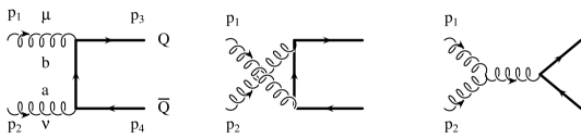
Figure 2: The $t$-, $u$- and $s$-shannel leading order (Born) graphs contributing to the gluon (curly lines) fusion amplitude. The thick solid lines correspond to the heavy quarks.

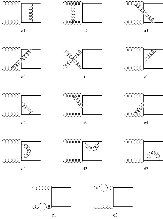
Figure 3: The $t$-channel one-loop graphs contributing to the gluon fusion amplitude. Loops with dotted lines represent gluon, ghost and light and heavy quarks.

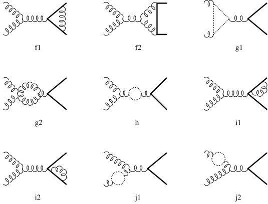
Figure 4: The $s$-channel one-loop graphs contributing to the gluon fusion amplitude. Loops with dotted lines as in g1,h,j1 and j2 represent gluon, ghost and light and heavy quarks. The four-gluon coupling contribution appears in g2.

In order to isolate ultraviolet (UV) and infrared/collinear (IR/M) divergences we have carried out all our calculations in the dimensional regularization scheme (DREG) DREG with the dimension of space-time being formally $n=4-2\varepsilon$.

First of all we note that in general the amplitudes for all the Feynman diagrams in the gluon fusion subprocess can be written in the form

$$M=\epsilon_{\mu}(p_{1})\epsilon_{\nu}(p_{2})\bar{u}(p_{3})M^{\mu\nu}v(p_{4}),$$ (8)

For purposes of brevity, we will present our results in terms of truncated amplitudes $M^{\mu\nu}$ where the polarization vectors and Dirac spinors are omitted. For reasons of brevity we shall also refer to the truncated amplitudes as amplitudes. Of course, the presence of the polarization vectors and Dirac spinors is implicitly understood throughout this paper in that the mass shell conditions $p_{1}^{\mu}\epsilon_{\mu}(p_{1})=0$ and $\not{\rm}p_{3}u(p_{3})=mu(p_{3})$ etc. are being used to simplify $M^{\mu\nu}$ . Furthermore, $M^{\mu\nu}$ contains the common factor $C_{\varepsilon}(m^{2})$ defined in Eq. (2) which arises from the scalar one-loop integrations described in KMR . Throughout the paper we will omit from all our one-loop $M^{\mu\nu}$ amplitudes the common factor

$$\mathcal{C}=g^{4}C_{\varepsilon}(m^{2}),$$ (9)

where $g$ is the renormalized coupling constant.

There are three sets of contributing graphs: The $t$–channel, $u$–channel and the $s$–channel graphs as exemplified in Fig. 2 for the LO Born term contributions. Since the $u$–channel amplitudes ${\mathcal{M}}_{u}$ can be obtained from the $t$–channel amplitudes ${\mathcal{M}}_{t}$ by the relation

$${\mathcal{M}}_{t}\leftrightarrow{\mathcal{M}}_{u}\equiv\{a\leftrightarrow b,\quad p_{1}\leftrightarrow p_{2},\quad\mu\leftrightarrow\nu\},$$ (10)

we shall not list results of the $u$–channel contributions. In (10) $a,b$ are the color indices of the two gluons. We make it clear from the outset that additional $u$-channel graphs are obtained from the relevant $t$-channel graphs by the interchange of the two external bosonic lines (not only momenta). In exception are the two vertex insertion diagrams (3c3) and (3c4) which will be discussed later on. All three interchanges (color, Lorentz indices and bosonic momenta) have to be done simultaneously. Note that the second interchange in (10) implies also the interchange $t\leftrightarrow u$. In general, when speaking about the $t$-$u$ symmetry of a given subset of amplitudes, we will imply invariance of those amplitudes under the transformations (10).

We start by writing down amplitudes for the leading order Born terms. For the $t$-channel gluon fusion subprocess (first graph in Fig. 2) we have:

$$B_{t}^{\mu\nu}=-iT^{b}T^{a}\gamma^{\mu}({\rm}\not p_{3}-{\rm}\not p_{1}+m)\gamma^{\nu}/t,$$

where $T^{b}$ and $T^{a}$ are generators ($T^{a}=\lambda^{a}/2$, $a=1,...,8$ and the $\lambda^{a}$ are the usual Gell-Mann matrices) that define the fundamental representation of the Lie algebra of the color SU(3) group. Analogously, for the $u$- and $s$-channels depicted in the second and third graph of Fig. 2 we have, respectively,

$$B_{u}^{\mu\nu} = -iT^{a}T^{b}\gamma^{\nu}({\rm}\not p_{3}-{\rm}\not p_{2}+m)\gamma^{\mu}/u,$$

$$B_{s}^{\mu\nu} = i(T^{a}T^{b}-T^{b}T^{a})C_{3}^{\mu\nu\sigma}\gamma_{\sigma}/s,$$

where the tensor $C_{3}^{\mu\nu\sigma}$ is obtained from the Feynman rules for the three-gluon coupling and is given by

$$C_{3}^{\mu\nu\sigma}=g_{\mu\nu}(p_{1}-p_{2})_{\sigma}+g_{\nu\sigma}(p_{1}+2p_{2})_{\mu}-g_{\mu\sigma}(2p_{1}+p_{2})_{\nu}.$$ (11)

We have omitted a common factor $g^{2}$ in the Born amplitudes. Acting with Dirac spinors $\bar{u}(p_{3})$ and $v(p_{4})$ on the above truncated Born amplitudes from the left and the right, respectively, and using the effective relations $p_{1}^{\mu}=p_{2}^{\nu}=0$, as remarked on before, we arrive at the following expressions for the leading order amplitudes:

$$B_{t}^{\mu\nu} = iT^{b}T^{a}(\gamma^{\mu}{\rm}\not p_{1}\gamma^{\nu}-2p_{3}^{\mu}\gamma^{\nu})/t;$$

$$B_{u}^{\mu\nu} = iT^{a}T^{b}(\gamma^{\nu}{\rm}\not p_{2}\gamma^{\mu}-2p_{3}^{\nu}\gamma^{\mu})/u;$$

$$B_{s}^{\mu\nu} = 2i(T^{a}T^{b}-T^{b}T^{a})(g^{\mu\nu}{\rm}\not p_{1}+p_{2}^{\mu}\gamma^{\nu}-p_{1}^{\nu}\gamma^{\mu})/s.$$

Next we proceed with the description of the two-point insertions to the amplitudes of the subprocess (3). But before we turn to the two-point functions one should mention that our choice of renormalization scheme will be a fixed flavor scheme throughout this paper. This implies that we have a total number of flavors $n_{f}=n_{lf}+1$, where $n_{lf}$ is the number of light (i.e. massless) flavors and the $``1"$ stands for the produced heavy flavor. Thus there will only be $n_{lf}$ light flavors involved/active in the $\beta$ function for the running a QCD coupling $\alpha_{s}$, and in the splitting functions that determine the evolution of the structure functions. When having massless particles in the loops we are using the standard $\overline{\rm MS}$ scheme, while the contribution of a heavy quark loop in the gluon self-energy with on-shell external legs is subtracted out entirely.

Consider first the two $t$-channel self-energy insertion graphs (3d2) and (3d3) in Fig. 3 with external legs on-shell. These graphs are very important as they determine the renormalization parameters in the quark sector. Throughout this paper we use the so called on-shell prescription for the renormalization of heavy quarks, the essential ingredients of which we describe in the following. When dealing with massive quarks one has to choose a parameter to which one renormalizes the heavy quark mass. It is natural to choose a quark pole mass for such a parameter – the only “stable” mass parameter in QCD. The condition on the renormalized heavy quark self-energy $\Sigma_{r}(\not p)$ is

$$\Sigma_{r}(\not p)|_{\not p=m}=0,$$ (12)

which removes the singular internal propagator in these self-energy insertion diagrams. This can be seen from the explicit result for the renormalized heavy quark external self-energy $\Sigma_{r}(\not p)$ e.g. in dimensional regularization scheme:

$$\Sigma_{r}(\not p)=ig^{2}\frac{C_{F}C_{\varepsilon}(m^{2})}{\varepsilon(1-2\varepsilon)}\left[\not p-m+\not p\frac{m^{2}-p^{2}}{p^{2}}\times\right.$$

$$\left.\left(1+\frac{m^{2}-p^{2}}{2p^{2}}(1-\varepsilon)\right)-m\frac{m^{2}-p^{2}}{p^{2}}(2-\varepsilon)\right].$$ (13)

The above condition (12) determines the mass renormalization constant $Z_{m}$. For the wave function renormalization we have used the usual condition (see e.g. Ref. Ellis )

$$\frac{\partial}{\partial{\rm}\not p}\Sigma_{r}(\not p)|_{\not p=m}=0,$$ (14)

which fully determines the wave function renormalization constant $Z_{2}$. Since the condition (14) is not mandatory in general, there is a freedom in determining the constant $Z_{2}$. Note that the condition (14) sets all external heavy quark self-energy insertion diagrams to zero, thus making the heavy quark case similar to the massless one in this regard. Below we list our expressions for the mass and wave function renormalization constants.

In the DREG scheme we arrive at the result

$$Z_{m}=1-g^{2}C_{F}C_{\varepsilon}(m^{2})\frac{3-2\varepsilon}{\varepsilon(1-2\varepsilon)}$$ (15)

which can be expanded in $\varepsilon$ to give

$$Z_{m} = 1-g^{2}C_{F}C_{\varepsilon}(m^{2})\left(\frac{3}{\varepsilon}+4+8\varepsilon+16\varepsilon^{2}+{\mathcal{O}}(\varepsilon^{3})\right),$$

$$Z_{2} = Z_{m},$$ (16)

where $C_{F}$=4/3 and we do not make a distinction which poles are of ultraviolet or IR/M origin as we did in KM . After the mass renormalization procedure is applied we obtain the final results for the two self-energy insertion graphs in the DREG scheme

$$M_{\rm(3d2)}^{\mu\nu} = M_{\rm(3d3)}^{\mu\nu}=-C_{F}B_{t}^{\mu\nu}\frac{3-2\varepsilon}{\varepsilon(1-2\varepsilon)}$$

$$= -C_{F}B_{t}^{\mu\nu}\left(\frac{3}{\varepsilon}+4+8\varepsilon+16\varepsilon^{2}+{\mathcal{O}}(\varepsilon^{3})\right).$$

From here on we will present only results for the $\varepsilon$ and $\varepsilon^{2}$ order contributions to the amplitudes.

After addition of the mass renormalization counterterm the contribution of the quark self-energy insertion graph (3d1) with external legs off-shell reads:

$$M_{\rm(3d1)}^{\mu\nu} = C_{F}B_{t}^{\mu\nu}\sum_{k=1}^{2}\varepsilon^{k}\left(-B_{1}^{(k)}t/T+4B_{1}^{(k)}m^{2}/t\right.$$ (18)

$$\left.+B_{1}^{(k-1)}t/T-k16m^{2}/t\right)$$

$$- iC_{F}T^{b}T^{a}m\gamma^{\mu}\gamma^{\nu}\sum_{k=1}^{2}\varepsilon^{k}\left(B_{1}^{(k)}/T+2B_{1}^{(k)}/t\right.$$

$$\left.-B_{1}^{(k-1)}/T-k8/t\right).$$

The coefficients $B_{1}^{(k)}$ and $B_{1}^{(k-1)}$ come from the Laurent series expansion of the scalar two-point function $B_{1}$ (see Table 1) quite similar to the corresponding Laurent series expansion of the four-point functions $D_{i}$ shown in Eq. (LABEL:Dexp).

The remaining quark self-energy insertion graphs (4i1) and (4i2) with external on-shell legs are derived in analogy to the ones considered above:

$$M_{\rm(4i1)}^{\mu\nu}=M_{\rm(4i2)}^{\mu\nu}=-C_{F}B_{s}^{\mu\nu}\left(8\varepsilon+16\varepsilon^{2}\right),$$ (19)

Concerning the gluon self-energy insertion graphs (3e1) and (3e2) with external legs on-shell, the only nonvanishing contributions are those from heavy quark loops. They are given by

$$M_{\rm(3e1)}^{\mu\nu}=M_{\rm(3e2)}^{\mu\nu}=-B_{t}^{\mu\nu}\frac{1}{\varepsilon}\,\,\frac{2}{3}.$$ (20)

However, these contributions are explicitly subtracted (together with the common factor $C_{\varepsilon}(m^{2})$, see Eqs. (2) and (9)) in the on-shell renormalization prescription. Therefore, due to the UV counterterm that subtracts this loop with heavy quarks, there are no finite contributions to the amplitudes from these self-energy diagrams. However, at the same time this counterterm introduces the pole terms from the light quark loop sector that are needed to cancel soft and collinear poles from the other parts of the amplitude, e.g. from the real bremsstrahlung part. This indicates that in practice it is very hard to completely disentangle UV and IR/M poles in heavy flavor production and in most cases one obtains a mixture of both instead.

For the reasons specified above we present the gauge field renormalization constant $Z_{3}$, used for the gluon self-energy subtraction:

$$Z_{3}=1+\frac{g^{2}}{\varepsilon}\left\{(\frac{5}{3}N_{C}-\frac{2}{3}n_{lf})C_{\varepsilon}(\mu^{2})-\frac{2}{3}C_{\varepsilon}(m^{2})\right\}$$

$$=1+\frac{g^{2}}{\varepsilon}\left\{(\beta_{0}-2N_{C})C_{\varepsilon}(\mu^{2})-\frac{2}{3}C_{\varepsilon}(m^{2})\right\},\quad$$ (21)

where the QCD beta–function $\beta_{0}=(11N_{C}-2n_{lf})/3$ contains only light quarks. $N_{C}=3$ is the number of colors. Accordingly, for the coupling contant renormalization we obtain

$$Z_{g}=1-\frac{g^{2}}{\varepsilon}\left\{\frac{\beta_{0}}{2}C_{\varepsilon}(\mu^{2})-\frac{1}{3}C_{\varepsilon}(m^{2})\right\}.$$ (22)

As was the case for the diagrams (3e1) and (3e2), diagrams (4j1) and (4j2) also vanish altogether due to the explicit decoupling of the heavy quarks in our subtraction prescription. However, instead of renormalizing separately each Feynman diagram, one can chose to employ the renormalization group invariance of the cross section and do only a mass and coupling constant renormalization. In this case, knowing the results for the gluon self-energy diagrams turns out to be useful in checking the complete cancellation of UV poles by just rescaling the coupling constant in the LO terms $g_{\rm bare}\rightarrow Z_{g}g$. One has

$$M_{\rm(4j1)}^{\mu\nu}=M_{\rm(4j2)}^{\mu\nu}=-B_{s}^{\mu\nu}\frac{1}{\varepsilon}\,\,\frac{2}{3}.$$ (23)

Finally we arrive at the gluon self-energy insertion graph (4h), which contains the off-shell gluon self-energy loop that is used for the derivation of the renormalization constant $Z_{3}$. We have evaluated the internal loop in the Feynman gauge. In our result we show separately the gauge invariant pieces for gluon plus ghost, light quarks and one heavy quark flow inside the loop:

$$M_{\rm(4h)}^{\mu\nu}=B_{s}^{\mu\nu}\left\{\frac{B_{5}}{iC_{\varepsilon}(m^{2})}\left[-N_{C}\frac{n-14+8\varepsilon}{2(3-2\varepsilon)}-n_{lf}\frac{2(1-\varepsilon)}{3-2\varepsilon}\right]\right.$$

$$\left.-\frac{1}{\varepsilon}\,\,\frac{2}{3}\,\,I\right\},\quad$$ (24)

with $n=4-2\varepsilon$ in the DREG scheme. $B_{5}$ is the two-point integral whose explicit form is given in KMR . We expand the first line of (II) in powers of $\varepsilon$ and find

$$M_{\rm(4h)}^{\mu\nu} = B_{s}^{\mu\nu}\left\{\left[N_{C}\left(\frac{1}{\varepsilon}\,\,\frac{5}{3}+\frac{31}{9}+\varepsilon\left(\frac{188}{27}-\frac{5}{3}\,\zeta(2)\right)\right.\right.\right.$$ (25)

$$\left.+\varepsilon^{2}\left(\frac{1132}{81}-\frac{31}{9}\,\zeta(2)-\frac{10}{3}\,\zeta(3)\right)\right)$$

$$-n_{lf}\left(\frac{1}{\varepsilon}\,\,\frac{2}{3}+\frac{10}{9}+\varepsilon\left(\frac{56}{27}-\frac{2}{3}\,\zeta(2)\right)\right.$$

$$\left.\left.+\varepsilon^{2}\left(\frac{328}{81}-\frac{10}{9}\,\zeta(2)-\frac{4}{3}\,\zeta(3)\right)\right)\right]\left(\frac{-s}{m^{2}}\right)^{-\varepsilon}$$

$$\left.-\frac{1}{\varepsilon}\,\,\frac{2}{3}\,\,I\right\},$$

with

$$I = 1+\varepsilon\left[-\frac{1}{3}+B_{2}^{(0)}\frac{3-\beta^{2}}{2}\right]$$

$$+\varepsilon^{2}\left[-\frac{2}{9}-\frac{1}{3}B_{2}^{(0)}\beta^{2}+B_{2}^{(1)}\frac{3-\beta^{2}}{2}\right]$$

$$+\varepsilon^{3}\left[-\frac{4}{27}-\frac{2}{9}B_{2}^{(0)}\beta^{2}-\frac{1}{3}B_{2}^{(1)}\beta^{2}+B_{2}^{(2)}\frac{3-\beta^{2}}{2}\right].$$

In (II) we have made use of the definition

$$\beta\equiv\sqrt{1-4m^{2}/s}.$$ (27)

Concluding our discussion on the 2-point insertions we remark that the amplitudes for the relevant u-channel 2-point insertion diagrams can be obtained from Eqs. (II), (18) and (20) by the transformation (10).

Next we discuss the $t$– and $u$–channel vertex insertions. In this paper we write down only the $\varepsilon$– and $\varepsilon^{2}$–terms of the Laurent expansion. The terms proportional to $\varepsilon^{-2}$, $\varepsilon^{-1}$ and $\varepsilon^{0}$ can be found in KM . We begin with the purely nonabelian graph (3b) with the four–gluon vertex. The amplitude takes the following form

$$M_{\rm(3b)}^{\mu\nu} = iN_{C}(T^{b}T^{a}\sum_{k=1}^{2}\varepsilon^{k}\{(2p_{3}^{\nu}\gamma^{\mu}+p_{4}^{\nu}\gamma^{\mu}-p_{3}^{\mu}\gamma^{\nu}-2p_{4}^{\mu}\gamma^{\nu})(B_{5}^{(k)}+2C_{1}^{(k)}m^{2}-4k)-mg^{\mu\nu}(2B_{5}^{(k)}+2B_{5}^{(k-1)}$$ (28)

$$+4C_{1}^{(k)}m^{2}+C_{1}^{(k-1)}s-12k)+3m\gamma^{\mu}\gamma^{\nu}(2B_{5}^{(k)}+C_{1}^{(k)}s-8k)/2\}/(s\beta^{2})+(a\leftrightarrow b,\mu\leftrightarrow\nu))$$

$$+ i\delta^{ab}\sum_{k=1}^{2}\varepsilon^{k}\{(p_{3}^{\nu}\gamma^{\mu}-p_{4}^{\nu}\gamma^{\mu}+p_{3}^{\mu}\gamma^{\nu}-p_{4}^{\mu}\gamma^{\nu})(B_{5}^{(k)}+2C_{1}^{(k)}m^{2}-4k)/2$$

$$+mg^{\mu\nu}(B_{5}^{(k)}-2B_{5}^{(k-1)}-4C_{1}^{(k)}m^{2}+3C_{1}^{(k)}s/2-C_{1}^{(k-1)}s)\}/(s\beta^{2}).$$

It is easily seen from Eq. (28) that the amplitude for the graph (3b) is explicitly $t$-$u$ symmetric, as it follows from the geometric topology of this graph. It is thus important to state that there is no $u$–channel equivalent of graph (3b).

Next we turn to graphs (3c1) and (3c2). As mentioned before, these diagrams occur also in other processes such as photoproduction and $\gamma\gamma$ production of heavy flavors when one or two of the gluons are replaced by photons. For this reason we also present the corresponding t-channel color factors for these graphs. Then it is straightforward to separate our Dirac structure from the color coefficients and one can easily deduce the corresponding results for the other processes involving photons. In order to facilitate this transscription we list the color factor for both diagrams (3c1) and (3c2) which turn out to be the same:

$$T_{\rm col}^{\rm(3c1)}=T_{\rm col}^{\rm(3c2)}=(C_{F}-\frac{N_{C}}{2})T^{b}T^{a}=-\frac{1}{6}T^{b}T^{a}.$$ (29)

The complete amplitudes are:

$$M_{\rm(3c1)}^{\mu\nu} = B_{t}^{\mu\nu}\sum_{k=1}^{2}\varepsilon^{k}\{B_{1}^{(k)}(6m^{2}/t+1)+2B_{1}^{(k-1)}z_{t}/t+2C_{2}^{(k)}m^{2}+4C_{2}^{(k-1)}m^{2}-k8(4m^{2}/t+1)\}/6$$ (30)

$$+ iT^{b}T^{a}(p_{3}^{\mu}\gamma^{\nu}\sum_{k=1}^{2}\varepsilon^{k}\{B_{1}^{(k)}(z_{t}/t+t/T)+B_{1}^{(k-1)}(2z_{t}/t-t/T)+2(C_{2}^{(k)}+2C_{2}^{(k-1)})m^{2}-k8z_{t}/t\}$$

$$+ mp_{3}^{\mu}{\rm}\not p_{1}\gamma^{\nu}\sum_{k=1}^{2}\varepsilon^{k}\{B_{1}^{(k)}/T-B_{1}^{(k-1)}(2/t+1/T)-2C_{2}^{(k-1)}+k4/t\}$$

$$- m\gamma^{\mu}\gamma^{\nu}\sum_{k=1}^{2}\varepsilon^{k}\{B_{1}^{(k)}+B_{1}^{(k-1)}+C_{2}^{(k-1)}t-6k\})/(3t),$$

where we have introduced the abbreviation $z_{t}\equiv 2m^{2}+t$.

For the graph (3c2) we obtain:

$$M_{\rm(3c2)}^{\mu\nu} = B_{t}^{\mu\nu}\sum_{k=1}^{2}\varepsilon^{k}\{B_{1}^{(k)}(6m^{2}/t+1)+2B_{1}^{(k-1)}z_{t}/t+2C_{2}^{(k)}m^{2}+4C_{2}^{(k-1)}m^{2}-k8(4m^{2}/t+1)\}/6$$ (31)

$$+ iT^{b}T^{a}(p_{4}^{\nu}\gamma^{\mu}\sum_{k=1}^{2}\varepsilon^{k}\{B_{1}^{(k)}(-2m^{2}/t-3+t/T)-B_{1}^{(k-1)}t/T-2C_{2}^{(k)}m^{2}+k8T/t\}$$

$$+ mp_{4}^{\nu}(2p_{3}^{\mu}-\gamma^{\mu}{\rm}\not p_{1})\sum_{k=1}^{2}\varepsilon^{k}\{B_{1}^{(k)}/T-B_{1}^{(k-1)}(2/t+1/T)-2C_{2}^{(k-1)}+k4/t\}$$

$$- m\gamma^{\mu}\gamma^{\nu}\sum_{k=1}^{2}\varepsilon^{k}\{B_{1}^{(k)}+B_{1}^{(k-1)}+C_{2}^{(k-1)}t-6k\})/(3t).$$

Next we write down the results for graphs (3c3) and (3c4). The color factors for both diagrams are the same:

$$T_{\rm col}^{\rm(3c3)}=T_{\rm col}^{\rm(3c4)}=-\frac{N_{C}}{2}T^{b}T^{a}=-\frac{3}{2}T^{b}T^{a}.$$ (32)

We have

$$M_{\rm(3c3)}^{\mu\nu} = 3B_{t}^{\mu\nu}\sum_{k=1}^{2}\varepsilon^{k}\{-3B_{1}^{(k)}m^{2}/t-C_{3}^{(k)}t$$ (33)

$$+k4(3m^{2}/t+1)\}$$

$$+3iT^{b}T^{a}(p_{3}^{\mu}\gamma^{\nu}\sum_{k=1}^{2}\varepsilon^{k}\{B_{1}^{(k)}m^{2}(1/T-2/t)$$

$$+B_{1}^{(k-1)}t/T-C_{3}^{(k)}t+k4z_{t}/t\}$$

$$+3m\gamma^{\mu}\gamma^{\nu}\sum_{k=1}^{2}\varepsilon^{k}\{B_{1}^{(k)}/2-2k\}$$

$$+mp_{3}^{\mu}{\rm}\not p_{1}\gamma^{\nu}\sum_{k=1}^{2}\varepsilon^{k}\{B_{1}^{(k)}(2/t-1/T)$$

$$+B_{1}^{(k-1)}/T-k8/t\})/t.$$

And

$$M_{\rm(3c4)}^{\mu\nu} = 3B_{t}^{\mu\nu}\sum_{k=1}^{2}\varepsilon^{k}\{-3B_{1}^{(k)}m^{2}/t-C_{3}^{(k)}t$$ (34)

$$+k4(3m^{2}/t+1)\}$$

$$+3iT^{b}T^{a}(p_{4}^{\nu}\gamma^{\mu}\sum_{k=1}^{2}\varepsilon^{k}\{B_{1}^{(k)}m^{2}(1/T-2/t)$$

$$+B_{1}^{(k-1)}(t/T-2)+C_{3}^{(k)}t+k4(2m^{2}/t-1)\}$$

$$+3m\gamma^{\mu}\gamma^{\nu}\sum_{k=1}^{2}\varepsilon^{k}\{B_{1}^{(k)}/2-2k\}$$

$$+mp_{4}^{\nu}(2p_{3}^{\mu}-\gamma^{\mu}{\rm}\not p_{1})\sum_{k=1}^{2}\varepsilon^{k}\{B_{1}^{(k)}(2/t-1/T)$$

$$+B_{1}^{(k-1)}/T-k8/t\})/t.$$

The results for the amplitudes of the relevant u-channel vertex insertion diagrams are obtained from Eqs. (30), (31), (33) and (34) by the transformation (10). However, there is a subtle point involved here: we stress that for the graphs (3c3) and (3c4) the $M_{t}\leftrightarrow M_{u}$ transformation (10) transforms the $t$-channel result of the graph (3c3) to the $u$-channel result for the graph (3c4), while the $t$-channel result of (3c4) goes to the $u$-channel result for (3c3). This is important to keep in mind when dealing with reactions which involve asymmetric set of graphs as e.g. in the photoproduction of heavy flavors. The reason for this is that when doing transformation (10) the three-gluon vertex attached to one of the initial bosonic lines does not stay attached to the same bosonic line. However, we note that transformation $p_{3}\leftrightarrow p_{4}$ does uniquely relate all the $t$- and $u$-channel diagrams for the subprocess under consideration.

Next we turn to the remaining $s$-channel graphs shown in Fig. 4. For all the gluon propagators we work in Feynman gauge. This set of graphs is purely nonabelian for the QCD type one-loop corrections. In the case that one wants to replace the gluonic vertex correction in graph (4f1) by a photonic vertex correction one needs the explicit form of the color factor for graph (4f1):

$$T_{\rm col}^{\rm(4f1)}=(C_{F}-\frac{N_{C}}{2})(T^{a}T^{b}-T^{b}T^{a})=-\frac{1}{6}(T^{a}T^{b}-T^{b}T^{a}).$$ (35)

The amplitude including the color factor is

$$M_{\rm(4f1)}^{\mu\nu} = B_{s}^{\mu\nu}\sum_{k=1}^{2}\varepsilon^{k}\{3B_{2}^{(k)}+2B_{2}^{(k-1)}+C_{6}^{(k)}s(1+\beta^{2})$$ (36)

$$-16k\}/6+2i(T^{a}T^{b}-T^{b}T^{a})m[-g^{\mu\nu}(s+2t)$$

$$-4p_{3}^{\mu}p_{4}^{\nu}+4p_{4}^{\mu}p_{3}^{\nu}]\sum_{k=1}^{2}\varepsilon^{k}\{B_{2}^{(k)}+2B_{2}^{(k-1)}-8k\}$$

$$/(6s^{2}\beta^{2}).$$

Graph (4f2) contributes as:

$$M_{\rm(4f2)}^{\mu\nu} = N_{C}B_{s}^{\mu\nu}\sum_{k=1}^{2}\varepsilon^{k}\{B_{5}^{(k)}(8m^{2}-s)+2C_{1}^{(k)}m^{2}s$$ (37)

$$-k16(5m^{2}-s)\}/(2s\beta^{2})$$

$$+2iN_{C}(T^{a}T^{b}-T^{b}T^{a})m[-g^{\mu\nu}(s+2t)-$$

$$4p_{3}^{\mu}p_{4}^{\nu}+4p_{4}^{\mu}p_{3}^{\nu}]\sum_{k=1}^{2}\varepsilon^{k}\{B_{5}^{(k)}(8m^{2}+s)$$

$$-2B_{5}^{(k-1)}s+6C_{1}^{(k)}m^{2}s-C_{1}^{(k-1)}s^{2}-$$

$$k4(12m^{2}-s)\}/2s^{3}\beta^{4}.$$

We end our consideration of the vertex insertions for gluonic fusion with the sum of the two graphs (4g1) and (4g2) which we refer to as the triangle graph contribution (tri)$\equiv$(4g1)+(4g2). For the case when one has gluons and ghosts inside the triangle loop we obtain:

$$M_{\rm(tri)}^{\mu\nu}(g) = -3N_{C}(B_{s}^{\mu\nu}\sum_{k=1}^{2}\varepsilon^{k}\{207B_{5}^{(k)}+12B_{5}^{(k-1)}$$ (38)

$$+54C_{4}^{(k)}s+8k+(k-1)8\tilde{B}_{5}^{(0)}\}$$

$$+6i(T^{a}T^{b}-T^{b}T^{a}){\rm}\not p_{1}\sum_{k=1}^{2}\varepsilon^{k}\{g^{\mu\nu}[9B_{5}^{(k)}$$

$$-12B_{5}^{(k-1)}+9C_{4}^{(k)}s-8k-(k-1)8\tilde{B}_{5}^{(0)}]/s$$

$$+8p_{2}^{\mu}p_{1}^{\nu}[3B_{5}^{(k-1)}+2k+(k-1)2\tilde{B}_{5}^{(0)}]/s^{2}\}$$

$$)/324,$$

where $\tilde{B}_{5}^{(0)}=B_{5}^{(0)}-4/3$. When one has light and heavy quarks inside the loop one has

$$M_{\rm(tri)}^{\mu\nu}(q) = 6n_{lf}(B_{s}^{\mu\nu}\sum_{k=1}^{2}\varepsilon^{k}\{9B_{5}^{(k)}-3B_{5}^{(k-1)}-2k$$ (39)

$$-(k-1)2\mathcal{B}_{5}^{(0)}\}-3i(T^{a}T^{b}-T^{b}T^{a}){\rm}\not p_{1}\times$$

$$[g^{\mu\nu}/s-2p_{2}^{\mu}p_{1}^{\nu}/s^{2}]\sum_{k=1}^{2}\varepsilon^{k}\{3B_{5}^{(k-1)}+5k$$

$$+(k-1)(5\tilde{B}_{5}^{(0)}+3)\})/81$$

where $n_{lf}$ is the number of light flavors in the triangle loop. For the heavy flavor case one has

$$M_{\rm(tri)}^{\mu\nu}(Q) = 6(B_{s}^{\mu\nu}\sum_{k=1}^{2}\varepsilon^{k}\{6(3B_{2}^{(k)}+2B_{2}^{(k-1)}+(k-1)4B_{2}^{(0)}/3)m^{2}/s+9B_{2}^{(k)}-3B_{2}^{(k-1)}-2k-2(k-1)\tilde{B}_{2}^{(0)}\}$$ (40)

$$-i(T^{a}T^{b}-T^{b}T^{a}){\rm}\not p_{1}[g^{\mu\nu}/s-2p_{2}^{\mu}p_{1}^{\nu}/s^{2}]\sum_{k=1}^{2}\varepsilon^{k}\{12(3B_{2}^{(k)}+2B_{2}^{(k-1)}+(k-1)4B_{2}^{(0)}/3)m^{2}/s$$

$$+18(C_{5}^{(k)}+C_{5}^{(k-1)}+(k-1)C_{5}^{(0)})m^{2}+3B_{2}^{(k-1)}+5k+(k-1)(5\tilde{B}_{2}^{(0)}+3)\})/81,$$

where $\tilde{B}_{2}^{(0)}=B_{2}^{(0)}-4/3$. The complete amplitude for the triangle (tri)$\equiv$(4g1)+(4g2) is the sum of the above three expressions (38), (39) and (40):

$$M_{\rm(tri)}^{\mu\nu}=M_{\rm(tri)}^{\mu\nu}(g)+M_{\rm(tri)}^{\mu\nu}(q)+M_{\rm(tri)}^{\mu\nu}(Q).$$ (41)

In Ref. Andrei one can find general results for the gluon triangle in any gauge and dimension. We have compared the first two terms in (41) with the corresponding expressions in Ref. Andrei and found complete agreement.

III RESULTS FOR THE BOX DIAGRAMS IN GLUON FUSION

In this section we describe the technically most involved derivation of the 4-point massive box diagrams. The four box graphs (3a1)–(3a4) contributing to the subprocess $g+g\rightarrow Q+\overline{Q}$ are depicted in Fig. 3. We have used Passarino-Veltman techniques passar to reduce tensor integrals to scalar ones where the scalar master integrals are taken from our previous publication KMR .

For each of the gluon fusion box diagrams we expand the truncated amplitude $M^{\mu\nu}$ in terms of a set of 20 Lorentz-Dirac covariants multiplied by the same number of invariant functions. In the reduction of the Lorentz-Dirac structure to this basic set of 20 covariants we have been making use of the mass shell conditions described in Sec. II. The 20 Lorentz-Dirac covariants are subdivided into eight subsets according to their Dirac structure. The 20 invariant functions multiplying the covariants are sorted according to the contributions of a basic set of functions $f_{i}^{(k)}$ (called basis functions) related to the scalar master integrals of KMR . The index $i$ runs over the members of the set of basis functions occuring in a particular graph. The index $k$ denotes the power of $\varepsilon$ which the basis function multiplies. The basis functions $f_{i}^{(k)}$ are multiplied by coefficient functions $b_{in}^{(j)}$ where the index pair $(n,j)$ identifies the covariant which the coefficient function multiplies. Note that the basis functions $f_{i}^{(k)}$ have been defined such that the coefficient functions $b_{in}^{(j)}$ do not depend on the index $k$. We thus cast the box amplitude into the following universal form:

$$M^{\mu\nu} = iT_{\rm col}\,\,\sum_{k=1}^{2}\varepsilon^{k}\{M_{\rm Bt}^{\mu\nu}\sum f_{i}^{(k)}b_{i1}^{(0)}$$

$$+ \not{p}_{1}[g^{\mu\nu}\sum f_{i}^{(k)}b_{i1}^{(1)}+p_{3}^{\mu}p_{3}^{\nu}\sum f_{i}^{(k)}b_{i2}^{(1)}+p_{3}^{\mu}p_{4}^{\nu}\sum f_{i}^{(k)}b_{i3}^{(1)}+p_{4}^{\mu}p_{3}^{\nu}\sum f_{i}^{(k)}b_{i4}^{(1)}+p_{4}^{\mu}p_{4}^{\nu}\sum f_{i}^{(k)}b_{i5}^{(1)}]$$

$$+ \gamma^{\mu}[p_{3}^{\nu}\sum f_{i}^{(k)}b_{i1}^{(2)}+p_{4}^{\nu}\sum f_{i}^{(k)}b_{i2}^{(2)}]+\gamma^{\nu}[p_{3}^{\mu}\sum f_{i}^{(k)}b_{i1}^{(3)}+p_{4}^{\mu}\sum f_{i}^{(k)}b_{i2}^{(3)}]+m\gamma^{\mu}\gamma^{\nu}\sum f_{i}^{(k)}b_{i1}^{(4)}$$

$$+ m\gamma^{\mu}{\rm}\not{p}_{1}[p_{3}^{\nu}\sum f_{i}^{(k)}b_{i1}^{(5)}+p_{4}^{\nu}\sum f_{i}^{(k)}b_{i2}^{(5)}]+m\gamma^{\nu}{\rm}\not{p}_{1}[p_{3}^{\mu}\sum f_{i}^{(k)}b_{i1}^{(6)}+p_{4}^{\mu}\sum f_{i}^{(k)}b_{i2}^{(6)}]$$

$$+ m[g^{\mu\nu}\sum f_{i}^{(k)}b_{i1}^{(7)}+p_{3}^{\mu}p_{3}^{\nu}\sum f_{i}^{(k)}b_{i2}^{(7)}+p_{3}^{\mu}p_{4}^{\nu}\sum f_{i}^{(k)}b_{i3}^{(7)}+p_{4}^{\mu}p_{3}^{\nu}\sum f_{i}^{(k)}b_{i4}^{(7)}+p_{4}^{\mu}p_{4}^{\nu}\sum f_{i}^{(k)}b_{i5}^{(7)}]\}$$

$$+ \{{\cal M}_{t}\leftrightarrow{\cal M}_{u}\}.$$

The symbol $\{{\cal M}_{t}\leftrightarrow{\cal M}_{u}\}$ at the end of Eq.(III) needs to be explained. It has the same meaning as the symbol ${\cal M}_{t}\leftrightarrow{\cal M}_{u}$ defined in Eq.(10) except that diagrams (3a3) and (3a4) are exempted from the sum. The crossed boxes (3a3) and (3a4) go into each other under the ${\cal M}_{t}\leftrightarrow{\cal M}_{u}$ operation. More exactly, for each of these diagrams, when one symmetrically interchanges the two bosonic lines (together with the appended three-gluon vertex) one arrives at the original box graph topology since these boxes represent diagrams of the so called non-planar topology. This becomes even more clear when one interchanges $p_{3}\leftrightarrow p_{4}$: In this case each of the two crossed box graphs is reflected into itself.

Taking parity into account one has altogether $2\cdot 2\cdot 2\cdot 2/2=8$ independent amplitudes and thus eight independent covariants for the process $g+g\rightarrow Q+\overline{Q}$ in $n=4$–dimensions. We have made no attempt to reduce the 20 (plus 3 from the $u$–channel contributions) covariants in (III) to a basic set of independent gauge invariant covariants. In fact, gauge invariance will be checked later on in terms of the expansion (III). At any rate, the number of independent gauge invariant covariants will very likely change going from $n=4$ to a general $n\neq 4$.

Depending on the type of the box graph one has a different number of terms in the $(i)$ summation in (III). These numbers as well as the set of basis functions $f_{i}^{(k)}$ related to the scalar master integrals are specified below. The coefficient functions $b_{in}^{(j)}$ are given in Appendix A of this paper.

In the expansion (III) it is convenient to choose one covariant as the t-channel Born term amplitude structure $M_{\rm Bt}^{\mu\nu}$ (and correspondingly a $u$–channel Born term amplitude structure). We define it as

$$M_{\rm Bt}^{\mu\nu}\equiv\gamma^{\mu}(\not{p}_{3}-\not{p}_{1}+m)\gamma^{\nu},$$ (43)

which, when taken between the spin wave functions implying the effective relations $p_{1}^{\mu}=0,\,\,p_{2}^{\nu}=0$, can be written as

$$M_{\rm Bt}^{\mu\nu}=2p_{3}^{\mu}\gamma^{\nu}-\gamma^{\mu}{\rm}\not{p}_{1}\gamma^{\nu}.$$ (44)

For each of the box diagrams (3a1) and (3a2) we found the following empirical relations between the $b_{in}^{(5)}$ and $b_{in}^{(6)}$ coefficient functions:

$$b_{i1}^{(6)}=b_{i2}^{(5)},\qquad b_{i2}^{(6)}=b_{i1}^{(5)}.$$ (45)

Because of the relations (45) we will not write down the results for the $b_{in}^{(6)}$ coefficients in the Appendix A.

Next we present the color factors and basis functions for the abelian type box diagram (3a1). For this graph the sums over $i$ in (III) run from 1 to 17 for each of the 20 terms. One has:

$$T_{\rm col}=\frac{1}{4}\delta^{ab}+(C_{F}-\frac{N_{C}}{2})T^{b}T^{a}.$$ (46)

$$f_{1}^{(k)}=B_{1}^{(k-1)},\qquad f_{2}^{(k)}=B_{1}^{(k)},\qquad f_{3}^{(k)}=B_{2}^{(k-1)},$$

$$f_{4}^{(k)}=B_{2}^{(k)},\qquad f_{5}^{(k)}=C_{2}^{(k-1)},\qquad f_{6}^{(k)}=C_{2}^{(k)},$$

$$f_{7}^{(k)}=C_{5}^{(k-1)},\qquad f_{8}^{(k)}=C_{5}^{(k)},\qquad f_{9}^{(k)}=C_{6}^{(k-1)},$$

$$f_{10}^{(k)}=C_{6}^{(k)},\qquad f_{11}^{(k)}=D_{1}^{(k-1)},\qquad f_{12}^{(k)}=D_{1}^{(k)},$$

$$f_{13}^{(k)}=k,$$ (47)

$$f_{14}^{(k)}=(k-1)C_{2}^{(k-2)},\qquad f_{15}^{(k)}=(k-1)C_{5}^{(k-2)},$$

$$f_{16}^{(k)}=(k-1)C_{6}^{(k-2)},\qquad f_{17}^{(k)}=(k-1)D_{1}^{(k-2)}.$$

The corresponding coefficient functions $b_{in}^{(j)}$ are listed in Appendix A. Many of the coefficient functions are in fact related to each other. One has

$$b_{12\,n}^{(j)}=-tb_{10\,n}^{(j)},\qquad j\neq 0.$$ (48)

And for any given values of $n$ and $j$ one has

$$b_{11\,n}^{(j)}=-tb_{9n}^{(j)},\qquad b_{15\,n}^{(j)}=s/(2t)b_{14\,n}^{(j)},$$ (49)

$$b_{16\,n}^{(j)}=s\beta^{2}/(2z_{t})b_{14\,n}^{(j)},\qquad b_{17\,n}^{(j)}=-st\beta^{2}/(2z_{t})b_{14\,n}^{(j)}.$$

Further relations are valid for particular sets of the parameters $n,j$:

$$b_{7n}^{(j)}=s/(2t)b_{5n}^{(j)},\qquad j=0,1,2,4;$$

$$b_{7n}^{(7)}=s/(2t)b_{5n}^{(7)},\qquad n=1,3,5;$$ (50)

$$b_{8n}^{(j)}=s/(2t)b_{6n}^{(j)},\qquad j=4,5,6,7.$$

Because of these relations among the coefficient functions we will write down only the independent coefficients $b_{in}^{(j)}$ in Appendix A.

For the nonabelian box diagram (3a2) the sums over $i$ in (III) again run from 1 to 17 for each of the 20 terms in (III) . For the color factor we obtain:

$$T_{\rm col}=\frac{1}{4}\delta^{ab}+\frac{N_{C}}{2}T^{b}T^{a}.$$ (51)

The relevant seventeen basis functions that describe the result of evaluating the box diagram (3a2) are given by

$$f_{1}^{(k)}=B_{1}^{(k-1)},\qquad f_{2}^{(k)}=B_{1}^{(k)},\qquad f_{3}^{(k)}=B_{5}^{(k-1)},$$

$$f_{4}^{(k)}=B_{5}^{(k)},\qquad f_{5}^{(k)}=C_{1}^{(k-1)},\qquad f_{6}^{(k)}=C_{1}^{(k)},$$

$$f_{7}^{(k)}=C_{3}^{(k-1)},\qquad f_{8}^{(k)}=C_{3}^{(k)},\qquad f_{9}^{(k)}=C_{4}^{(k-1)},$$

$$f_{10}^{(k)}=C_{4}^{(k)},\qquad f_{11}^{(k)}=D_{2}^{(k-1)},\qquad f_{12}^{(k)}=D_{2}^{(k)},$$

$$f_{13}^{(k)}=k,$$ (52)

$$f_{14}^{(k)}=(k-1)C_{1}^{(k-2)},\qquad f_{15}^{(k)}=(k-1)C_{3}^{(k-2)},$$

$$f_{16}^{(k)}=(k-1)C_{4}^{(k-2)},\qquad f_{17}^{(k)}=(k-1)D_{2}^{(k-2)}.$$

There are five relations between particular coefficients for the box diagram (3a2), valid for any values of $n$ and $j$:

$$b_{9n}^{(j)}=s/(2t)b_{7n}^{(j)},\qquad b_{11n}^{(j)}=-(s/2)b_{7n}^{(j)},$$ (53)

and

$$b_{14n}^{(j)}=sz_{t}/(2t^{2})b_{15n}^{(j)},\qquad b_{16n}^{(j)}=s/(2t)b_{15n}^{(j)},$$

$$b_{17n}^{(j)}=-(s/2)b_{15n}^{(j)}.$$ (54)

In addition, one has two sets of relations that are valid for the corresponding parts of the expression (III) for the box (3a2). The first set of relations is

$$b_{5n}^{(j)}=sz_{t}/(2t^{2})b_{7n}^{(j)},$$ (55)

$$b_{14n}^{(j)}=2b_{5n}^{(j)},\qquad b_{15n}^{(j)}=2b_{7n}^{(j)},$$ (56)

$$b_{16n}^{(j)}=2b_{9n}^{(j)},\qquad b_{17n}^{(j)}=2b_{11n}^{(j)},$$

The above equalities are valid for $j=0,2,3,4,5,6$ and for $j=1,7\,\,and\,\,n=1$. Note that in the presence of the set (III) not all of the relations in (55), (56) are independent. Therefore, we can choose Eq. (55) and only one relation (e.g. the second one) out of the four relations in (56) as a set of independent relations.

The second set of relations is represented by the two equalities that are identical to the ones of (53), but are valid only for $j=4,5,6,7$ or for $j=1\,\,and\,\,n=2,3,4,5$:

$$b_{10n}^{(j)}=s/(2t)b_{8n}^{(j)},\qquad b_{12n}^{(j)}=-(s/2)b_{8n}^{(j)},$$ (57)

In the case of the crossed box (3a4) one has twenty basis functions for each of the terms in (III). The color factor for this graph takes the simple form

$$T_{\rm col}=\frac{1}{4}\delta^{ab}.$$ (58)

The functions $f_{i}^{k}$ are defined as follows:

$$f_{1}^{(k)}=B_{1}^{(k-1)},\qquad f_{2}^{(k)}=B_{1}^{(k)},$$

$$f_{3}^{(k)}=B_{1u}^{(k-1)},\qquad f_{4}^{(k)}=B_{1u}^{(k)},$$

$$f_{5}^{(k)}=C_{2}^{(k-1)},\qquad f_{6}^{(k)}=C_{2}^{(k)},$$

$$f_{7}^{(k)}=C_{2u}^{(k-1)},\qquad f_{8}^{(k)}=C_{2u}^{(k)},$$

$$f_{9}^{(k)}=C_{3}^{(k-1)},\qquad f_{10}^{(k)}=C_{3}^{(k)},$$

$$f_{11}^{(k)}=C_{3u}^{(k-1)},\qquad f_{12}^{(k)}=C_{3u}^{(k)},$$

$$f_{13}^{(k)}=D_{3}^{(k-1)},\qquad f_{14}^{(k)}=D_{3}^{(k)},$$

$$f_{15}^{(k)}=k,$$ (59)

$$f_{16}^{(k)}=(k-1)C_{2}^{(k-2)},\qquad f_{17}^{(k)}=(k-1)C_{2u}^{(k-2)},$$

$$f_{18}^{(k)}=(k-1)C_{3}^{(k-2)},\qquad f_{19}^{(k)}=(k-1)C_{3u}^{(k-2)},$$

$$f_{20}^{(k)}=(k-1)D_{3}^{(k-2)},$$

where the subscript “u” is an operational definition prescribing a $(t\leftrightarrow u)$ interchange in the argument of that function, i.e. $B_{1u}^{(k)}=B_{1}^{(k)}(t\leftrightarrow u)$.

There are numerous relations between the $b_{in}^{(j)}$ coefficient functions for this diagram. These relations read:

For any value of $n$ and $j$

$$b_{11\,n}^{(j)}=b_{9n}^{(j)}u/t,\qquad b_{13\,n}^{(j)}=-b_{9n}^{(j)}u,$$ (60)

as well as

$$b_{7n}^{(j)}=b_{5n}^{(j)}u/t,\qquad j\neq 5;$$ (61)

$$b_{8n}^{(j)}=b_{6n}^{(j)}u/t,\qquad j\neq 1,2;$$

$$b_{12\,n}^{(j)}=b_{10\,n}^{(j)}u/t,\qquad j=4,5,6,7;$$

$$b_{12\,n}^{(1)}=b_{10\,n}^{(1)}u/t,\qquad n\neq 1;$$

$$b_{14\,n}^{(1)}=-b_{12\,n}^{(1)}t,\qquad n\neq 0,2;$$

$$b_{14,2}^{(2)}=-b_{12,2}^{(2)}t.\qquad\qquad\qquad$$

Further one has a less general but still very useful relation for any $n$

$$b_{9n}^{(j)}=-b_{5n}^{(j)}tu/(2D+tu),\qquad j=0,3,6,$$ (62)

with $D=m^{2}s-tu$. Equation (62) above is also valid for $j=1,7$ and $n=1$.

For the coefficient functions that effectively only multiply the $\varepsilon^{2}$–terms we have two sets of relations. One set is

$$b_{16\,n}^{(j)}=2b_{5n}^{(j)},$$ (63)

$$b_{17\,n}^{(j)}=2b_{7n}^{(j)},\qquad b_{18\,n}^{(j)}=2b_{9n}^{(j)},$$

$$b_{19\,n}^{(j)}=2b_{11\,n}^{(j)},\qquad b_{20\,n}^{(j)}=2b_{13\,n}^{(j)}\,$$

which are valid for the same values of $j,n$ as specified in and after (62). The other set reads

$$b_{17\,n}^{(j)}=b_{16\,n}^{(j)}u/t,$$ (64)

$$b_{18\,n}^{(j)}=-b_{16\,n}^{(j)}tu/(2D+tu),$$

$$b_{19\,n}^{(j)}=-b_{16\,n}^{(j)}u^{2}/(2D+tu),$$

$$b_{20\,n}^{(j)}=b_{16\,n}^{(j)}tu^{2}/(2D+tu).$$

The relations (64) are global for the crossed box (3a4), i.e. valid for any set of index values. Because the relations (63) always occur together with the relations (62), only the first relation of (63) is important. The other four relations in (63) are redundant since they can be derived from (60), the first relation in (61), (62) and (64).

In addition to the relations listed above, various coefficient functions of the crossed box are related by $(t\leftrightarrow u)$ exchange. For instance, the coefficient functions multiplying the Born term structure $M_{\rm Bt}^{\mu\nu}$ (or $j=0$) are related by

$$b_{i,1}^{(0)}=b_{i+2,1}^{(0)}(t\leftrightarrow u), \quad i=1,2,5,6,9,10;$$ (65)

$$b_{i,1}^{(0)}=b_{i+1,1}^{(0)}(t\leftrightarrow u), \quad i=16,18;$$

The remaining $(j=0)$ coefficient functions turn into themselves under $(t\leftrightarrow u)$.

Figure 5: The lowest order Feynman diagram contributing to the subprocess $q\bar{q}\rightarrow Q\overline{Q}$. The thick lines correspond to the heavy quarks.

Other coefficient functions are negatively related by $(t\leftrightarrow u)$–exchange:

$$b_{i,4}^{(1)}=-b_{i+2,3}^{(1)}(t\leftrightarrow u), \quad i=1,2,5,6,9,10;$$

$$b_{i,4}^{(1)}=-b_{i,3}^{(1)}(t\leftrightarrow u), \quad i=13,14,15,20;$$

$$b_{i,4}^{(1)}=-b_{i+1,3}^{(1)}(t\leftrightarrow u), \quad i=16,18.$$

$$b_{i,5}^{(1)}=-b_{i+2,2}^{(1)}(t\leftrightarrow u), \quad i=1,2,5,6,9,10;$$

$$b_{i,5}^{(1)}=-b_{i,2}^{(1)}(t\leftrightarrow u), \quad i=13,14,15,20;$$

$$b_{i,5}^{(1)}=-b_{i+1,2}^{(1)}(t\leftrightarrow u), \quad i=16,18.$$

Furthermore, the whole term corresponding to $j=4$ in (III) is antisymmetric under $(t\leftrightarrow u)$. The following pairs of coefficient functions are negatively related in the sense of (III): the $b_{i2}^{(5)}$ are related to $b_{l1}^{(5)}$, and the $b_{i2}^{(6)}$ are related to $b_{l1}^{(6)}$, where $l$ can take any of the values $l=i,i+1,i+2$ depending on the value of $i$. The number of independent coefficient functions is greatly reduced for this box because of all these relations. We took advantage of this fact when writing down the relevant coefficient functions in Appendix A.

As explained after Eq. (III) the crossed box (3a4) is obtained from (3a3) with the help of the ${\cal M}_{t}\leftrightarrow{\cal M}_{u}$ operation. For this reason we write down explicit results only for one of the box (3a3) in Appendix. A.

A necessary check on the correctness of our one–loop results is gauge invariance. For example, for gluon 1 this implies that one must have

$$p_{1\mu}\epsilon_{\nu}(p_{2})\bar{u}(p_{3})M^{\mu\nu}({\rm one-loop})v(p_{4})=0,$$ (67)

for each of the remaining independent amplitude structures that multiply e.g. $p_{1\nu}$, $p_{3\nu}$ and $\gamma_{\nu}$. Similarly one must have

$$p_{2\nu}\epsilon_{\mu}(p_{1})\bar{u}(p_{3})M^{\mu\nu}({\rm one-loop})v(p_{4})=0$$ (68)

again, for each of the remaining independent amplitude structures that multiply e.g. $p_{2\mu}$, $p_{3\mu}$ and $\gamma_{\mu}$. We have verified gauge invariance for the following gauge-invariant subsets of diagrams: (i) When the incoming gauge bosons are photons, i.e. including graphs (3a1), (3c1), (3c2), (3d1), (3d2), (3d3) plus their u-channel counterparts with their corresponding color weights; (ii) For the photoproduction of heavy flavors, i.e. including all the above diagrams plus graphs (3a4), (3c4), (3e1) plus their u-channel counterparts, with corresponding color weights; (iii) For the hadroproduction of heavy flavors, which ultimately includes all the graphs from Figs. 3 and 4 plus their relevant u-channel counterparts. We emphasize that the above gauge invariance checks were made separately for both color structures $C_{F}$ and $N_{C}$, and for every existing combination of color matrices $T^{a}$, $T^{b}$ and $\delta^{ab}$, whenever they arise. When checking on gauge invariance all the relevant $s$-, $t$- and $u$-channel graphs have to be added. Gauge invariance must of course be checked for each power of $\varepsilon$ and for each of the coefficient functions of the Laurent series expansion of the scalar master integrals separately, independent of their actual numerical values.

Finally we note that the original computer output for the box diagrams was extremely long. The final results were cast into the above shorter form with the help of the REDUCE Computer Algebra System reduce .

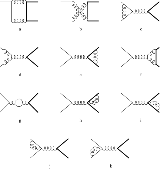
Figure 6: The one-loop Feynman diagrams contributing to the subprocess $q\bar{q}\rightarrow Q\overline{Q}$. The loop with dotted line represents gluon, ghost and light and heavy quarks.

IV ANNIHILATION OF THE QUARK-ANTIQUARK PAIR

The LO Born graphs contributing to this subprocess are shown in Fig. 5. In Fig. 6 we show the graphs contributing at one-loop order.

The leading order contribution proceeds only through the s-channel graph. One has:

$$B_{q\bar{q}}=iT^{a}_{ij}T^{a}_{kl}\bar{v}(p_{2})\gamma^{\mu}u(p_{1})\bar{u}(p_{3})\gamma_{\mu}v(p_{4})/s.$$ (69)

Here the color matrices $T^{a}$ belong to different fermion lines which are connected by the gluon having color index $a$. We have again left out the factor $g^{2}$ in the Born term contribution (69). In the Passarino-Veltman reduction for tensor integrals we can make use of the same scalar integrals of KMR as those appearing in the gluon fusion subprocess, with relevant shifts and interchanges of momenta when needed.

Starting again with the 2-point insertions, we notice that the result for graph (6g) can be obtained from the one of (25) for graph (4h) in the gluon fusion subprocess by the simple replacement

$$M_{(6\rm g)}=M_{(4\rm h)}^{\mu\nu}\,(B_{s}^{\mu\nu}\rightarrow B_{q\bar{q}}).$$ (70)

The massless quark self-energy insertion graphs (6j) and (6k) with external legs on-shell vanish identically:

$$M_{(6\rm j)}=M_{(6\rm k)}=0.$$ (71)

The massive quark self-energy insertion graphs (6h) and (6i) with external legs on-shell are calculated in analogy to the ones considered in the previous section:

$$M_{\rm(6h)}=M_{\rm(6i)}=-C_{F}B_{q\bar{q}}\frac{3-2\varepsilon}{\varepsilon(1-2\varepsilon)}\,.$$ (72)

The results for the vertex insertions are relatively short. Starting with graphs (6c) and (6d) one finds that they are proportional to the LO Born term:

$$M_{(6\rm c)}=B_{q\bar{q}}\sum_{k=1}^{2}\varepsilon^{k}\{3B_{5}^{(k)}+2B_{5}^{(k-1)}+2C_{4}^{(k)}s\}/6$$ (73)

and

$$M_{(6\rm d)}=-3B_{q\bar{q}}\sum_{k=1}^{2}\varepsilon^{k}B_{5}^{(k)}/2.$$ (74)

For the other two vertex insertion diagrams we also obtain simple expressions:

$$M_{(6\rm e)} = (B_{q\bar{q}}\sum_{k=1}^{2}\varepsilon^{k}\{3B_{2}^{(k)}+2B_{2}^{(k-1)}+C_{6}^{(k)}s(1+\beta^{2})$$

$$-16k\}+4iT^{a}T^{a}m\bar{v}(p_{2}){\rm}\not p_{3}u(p_{1})\bar{u}(p_{3})v(p_{4})\times$$

$$\sum_{k=1}^{2}\varepsilon^{k}\{B_{2}^{(k)}+2B_{2}^{(k-1)}-8k\}/(s^{2}\beta^{2}))/6$$

and

$$M_{(6\rm f)} = 3(B_{q\bar{q}}\sum_{k=1}^{2}\varepsilon^{k}\{B_{5}^{(k)}(8m^{2}/s-1)+2C_{1}^{(k)}m^{2}$$ (76)

$$-k16(5m^{2}/s-1)\}+4iT^{a}T^{a}m\bar{v}(p_{2}){\rm}\not p_{3}u(p_{1})\times$$

$$\bar{u}(p_{3})v(p_{4})\sum_{k=1}^{2}\varepsilon^{k}\{B_{5}^{(k)}(8m^{2}/s+1)-2B_{5}^{(k-1)}$$

$$+6C_{1}^{(k)}m^{2}-C_{1}^{(k-1)}s-k4(12m^{2}/s-1)\}$$

$$/(s^{2}\beta^{2}))/(2\beta^{2}).$$

Turning to the two box diagrams (6a) and (6b) we note that extensive Dirac algebra manipulations lead to rather compact expressions for the amplitudes. We have expanded the box diagrams in terms of seven independent Dirac structures, the same set for each of the two box graphs. Then every Dirac structure is multiplied by the sums of products of a small set of basis functions and coefficient functions. Thus, we have the following compact expansion for the two box diagrams:

$$M = iT_{\rm col}\sum_{k=1}^{2}\varepsilon^{k}\left\{\bar{v}(p_{2})\gamma^{\mu}u(p_{1})\bar{u}(p_{3})\gamma_{\mu}v(p_{4})\sum f_{i}^{(k)}h_{i}^{(0)}\right.$$

$$+ \bar{v}(p_{2}){\rm}\not p_{3}u(p_{1})\bar{u}(p_{3}){\rm}\not p_{1}v(p_{4})\sum f_{i}^{(k)}h_{i}^{(1)}$$

$$+ \bar{v}(p_{2})\gamma^{\nu}{\rm}\not p_{3}\gamma^{\mu}u(p_{1})\bar{u}(p_{3})\gamma_{\mu}{\rm}\not p_{1}\gamma_{\nu}v(p_{4})\sum f_{i}^{(k)}h_{i}^{(2)}$$

$$+ \bar{v}(p_{2})\gamma^{\nu}\gamma^{\alpha}\gamma^{\mu}u(p_{1})\bar{u}(p_{3})\gamma_{\mu}\gamma_{\alpha}\gamma_{\nu}v(p_{4})\sum f_{i}^{(k)}h_{i}^{(3)}$$

$$+ m\bar{v}(p_{2}){\rm}\not p_{3}u(p_{1})\bar{u}(p_{3})v(p_{4})\sum f_{i}^{(k)}h_{i}^{(4)}$$

$$+ m\bar{v}(p_{2})\gamma^{\mu}u(p_{1})\bar{u}(p_{3})\gamma_{\mu}{\rm}\not p_{1}v(p_{4})\sum f_{i}^{(k)}h_{i}^{(5)}$$

$$+ \left.m\bar{v}(p_{2})\gamma^{\nu}{\rm}\not p_{3}\gamma^{\mu}u(p_{1})\bar{u}(p_{3})\gamma_{\mu}\gamma_{\nu}v(p_{4})\sum f_{i}^{(k)}h_{i}^{(6)}\right\}.$$

There are seven independent covariants in (IV) upon using the four mass–shell conditions. We have not attempted to further reduce the set of seven covariants using Fierz–type identities which are anyway valid only in $n=4$–dimensions. Taking parity and the masslessness of the initial quarks into account the number of amplitudes and thereby the number of independent covariants in $n=4$ is $2\cdot 2\cdot 2\cdot 2/2\cdot 2=4$. However, this counting may no longer be true in $n\neq 4$.

The sums over $i$ in (IV) run from 1 to 15 in the box diagram (6a). Below we list the color factors and analytic functions for the two 4-point functions of (IV). For the graph (6a) we get:

$$T_{\rm col}=(T^{a}_{im}T^{b}_{mj})(T^{b}_{kn}T^{a}_{nl}),$$ (78)

where the first parentheses in (78) corresponds to the summation over color indices of the massless fermion line. The basis functions read

$$f_{1}^{(k)}=B_{1}^{(k)},\qquad f_{2}^{(k)}=B_{5}^{(k)},$$ (79)

$$f_{3}^{(k)}=C_{1}^{(k-1)},\qquad f_{4}^{(k)}=C_{1}^{(k)},\qquad f_{5}^{(k)}=C_{3}^{(k-1)},$$

$$f_{6}^{(k)}=C_{3}^{(k)},\qquad f_{7}^{(k)}=C_{4}^{(k-1)},\qquad f_{8}^{(k)}=C_{4}^{(k)},$$

$$f_{9}^{(k)}=D_{2}^{(k-1)},\qquad f_{10}^{(k)}=D_{2}^{(k)},\qquad f_{11}^{(k)}=k,$$

$$f_{12}^{(k)}=(k-1)C_{1}^{(k-2)},\qquad f_{13}^{(k)}=(k-1)C_{3}^{(k-2)},$$

$$f_{14}^{(k)}=(k-1)C_{4}^{(k-2)},\qquad f_{15}^{(k)}=(k-1)D_{2}^{(k-2)}.$$

As in the case of the gluon fusion boxes there exist a number of universal relations among the various coefficient functions $h_{i}^{(j)}$ valid for any value of $j$:

$$h_{3}^{(j)}=z_{t}h_{7}^{(j)}/t,\quad h_{5}^{(j)}=2th_{7}^{(j)}/s,\quad h_{9}^{(j)}=-th_{7}^{(j)},$$

$$h_{10}^{(j)}=-th_{8}^{(j)},\quad h_{12}^{(j)}=2z_{t}h_{7}^{(j)}/t,\quad h_{13}^{(j)}=4th_{7}^{(j)}/s,$$

$$h_{14}^{(j)}=2h_{7}^{(j)},\quad h_{15}^{(j)}=-2th_{7}^{(j)}$$ (80)

The color factor for the second box graph (6b) is

$$T_{\rm col}=(T^{a}T^{b})(T^{a}T^{b}).$$ (81)

All basis functions are obtained from those in (79) by the interchange $(t\leftrightarrow u)$, except for the two additional functions (with subscripts 16 and 17), e.g.:

$$f_{1}^{(k)}=B_{1}^{(k)}(t\leftrightarrow u),\qquad f_{2}^{(k)}=B_{5}^{(k)},$$ (82)

$$f_{3}^{(k)}=C_{1}^{(k-1)},\qquad f_{4}^{(k)}=C_{1}^{(k)},$$

$$f_{5}^{(k)}=C_{3}^{(k-1)}(t\leftrightarrow u),\qquad f_{6}^{(k)}=C_{3}^{(k)}(t\leftrightarrow u),$$

$$\qquad f_{7}^{(k)}=C_{4}^{(k-1)},\qquad f_{8}^{(k)}=C_{4}^{(k)},$$

$$f_{9}^{(k)}=D_{2}^{(k-1)}(t\leftrightarrow u),\qquad f_{10}^{(k)}=D_{2}^{(k)}(t\leftrightarrow u),$$

$$f_{11}^{(k)}=k,$$

$$f_{12}^{(k)}=(k-1)C_{1}^{(k-2)},\quad f_{13}^{(k)}=(k-1)C_{3}^{(k-2)}(t\leftrightarrow u),$$

$$f_{14}^{(k)}=(k-1)C_{4}^{(k-2)},\quad f_{15}^{(k)}=(k-1)D_{2}^{(k-2)}(t\leftrightarrow u),$$

$$f_{16}^{(k)}=B_{1}^{(k-1)}(t\leftrightarrow u),\qquad f_{17}^{(k)}=B_{5}^{(k-1)}.$$

The last two functions $f_{16}$ and $f_{17}$ appear in the expansion (IV) only in two sums where $h_{i}^{(1)}$ and $h_{i}^{(4)}$ are present and, consequently, these sums run from 1 to 17.

One has further relations for the various coefficient functions $h_{i}^{(j)}$ which are similar to those in Eq. (IV). In this case they are valid for any given value of $j$ except for $j=1$ and $j=4$.

$$h_{3}^{(j)}=z_{u}h_{7}^{(j)}/u,\quad h_{5}^{(j)}=2uh_{7}^{(j)}/s,\quad h_{9}^{(j)}=-uh_{7}^{(j)},$$

$$h_{10}^{(j)}=-uh_{8}^{(j)},\quad h_{12}^{(j)}=2z_{u}h_{7}^{(j)}/u,\quad h_{13}^{(j)}=4uh_{7}^{(j)}/s,$$

$$h_{14}^{(j)}=2h_{7}^{(j)},\quad h_{15}^{(j)}=-2uh_{7}^{(j)},$$ (83)

where $z_{u}=2m^{2}+u$. In case of $j=1$ and $j=4$ one has

$$h_{5}^{(j)}=2uh_{7}^{(j)}/s,\quad h_{9}^{(j)}=-uh_{7}^{(j)},\quad h_{10}^{(j)}=-uh_{8}^{(j)},$$

$$h_{12}^{(j)}=z_{u}h_{14}^{(j)}/u,\quad h_{13}^{(j)}=2uh_{14}^{(j)}/s,$$

$$h_{15}^{(j)}=-uh_{14}^{(j)}.$$ (84)

The coefficient functions $h_{i}^{(j)}$ are given in Appendix B of this paper. However, there exists a partial symmetry for these box diagrams, which allows one to express most coefficient functions for the box graph (6b) through the ones of the box graph (6a). In particular, starting from the coefficients $h_{i}^{(j)}$ with superscript $j\geq 2$, we find the following general relations:

$$h_{i}^{(j)}[{\rm(\ref{fig:qqnlo}b)}] = -h_{i}^{(j)}[{\rm(\ref{fig:qqnlo}a)}](t\leftrightarrow u),\quad j=2;$$ (85)

$$h_{i}^{(j)}[{\rm(\ref{fig:qqnlo}b)}] = h_{i}^{(j)}[{\rm(\ref{fig:qqnlo}a)}](t\leftrightarrow u),\quad j=3,5,6.$$

Consequently, for the graph (6b) only the coefficients $h_{i}^{(0)}$, $h_{i}^{(1)}$ and $h_{i}^{(4)}$ are presented in Appendix B. We reiterate that all the one-loop amplitudes of this chapter must be multiplied by the common factor (9).

V CONCLUSIONS

We have presented analytic ${\mathcal{O}}(\varepsilon^{2})$ results on the one-loop amplitudes for gluon– and light quark–induced heavy quark pair production including their absorptive parts . These are needed for the calculation of the loop-by-loop part of the parton model description of NNLO heavy hadron production in hadronic collisions. We have not included the finite and divergent pieces in our presentation since these were already obtained in an earlier publication KM . The advantage of having the results in amplitude form is that one retains the full spin information of the partonic subprocess which would be of later use when one wants to consider polarization phenomena in heavy hadron production. As an immediate next step we plan to square the one–loop amplitudes and to sum over the spins of the external partons. This will provide the necessary input for the loop-by-loop part of the NNLO parton model description of unpolarized heavy hadron or top quark pair production which is presently under study at the TEVATRON II and will be studied at the upcoming hadron collider LHC.

Appendix A

Here we present the coefficients of the box contributions for the gluon fusion subprocess appearing in Eq. (III).

We define a shorthand notation:

$$z_{1}\equiv m^{2}s-t^{2},\qquad z_{2}\equiv s+2t,$$

$$z_{t}\equiv 2m^{2}+t,\qquad z_{u}\equiv 2m^{2}+u,$$ (86)

$$D\equiv m^{2}s-ut.$$

First we list coefficients for the abelian type of box diagram (3a1):

$$b_{i,1}^{(0)}=0,\qquad i=1,2,3,4,13,$$

$$b_{5,1}^{(0)}=-10tz_{t}/D,\qquad b_{6,1}^{(0)}=2tz_{u}/D,$$

$$b_{8,1}^{(0)}=sz_{u}/D,\qquad b_{9,1}^{(0)}=-5st\beta^{2}/D,$$

$$b_{10,1}^{(0)}=-su_{1}\beta^{2}/D,\qquad b_{12,1}^{(0)}=s(D+m^{2}s\beta^{2})/D,$$

$$b_{14,1}^{(0)}=-24tz_{t}/D;$$

$$b_{1,1}^{(1)}=0,\qquad b_{2,1}^{(1)}=-2z_{t}^{2}/tD,\qquad b_{3,1}^{(1)}=0,$$

$$b_{4,1}^{(1)}=2z_{t}/D,\qquad b_{5,1}^{(1)}=2tz_{t}(6D+st\beta^{2})/D^{2},$$

$$b_{6,1}^{(1)}=-2z_{t}(2m^{2}D-st^{2}\beta^{2})/D^{2},$$

$$b_{8,1}^{(1)}=(2m^{2}z_{2}D+s^{2}tz_{t}\beta^{2})/D^{2},$$

$$b_{9,1}^{(1)}=s\beta^{2}/(2z_{t})b_{5,1}^{(1)},\qquad b_{10,1}^{(1)}=s^{2}t^{2}\beta^{4}/D^{2},$$

$$b_{13,1}^{(1)}=16m^{2}z_{t}/tD,\qquad b_{14,1}^{(1)}=4tz_{t}(6D+st\beta^{2})/D^{2};$$

$$b_{1,2}^{(1)}=4Tu\beta^{2}/D^{2},$$

$$b_{2,2}^{(1)}=-4m^{2}(2D^{2}+2t^{2}D+st(D-2t^{2})\beta^{2})/st^{2}D^{2},$$

$$b_{3,2}^{(1)}=4tuz_{t}/sD^{2},\qquad b_{4,2}^{(1)}=4m^{2}(D-2sz_{t})/sD^{2},$$

$$b_{5,2}^{(1)}=4tz_{t}(2m^{2}D-t(D+m^{2}s)\beta^{2})/D^{3},$$

$$b_{6,2}^{(1)}=-8m^{2}(T(sT-2m^{2}t)D+st^{3}z_{t}\beta^{2})/tD^{3},$$

$$b_{8,2}^{(1)}=4m^{2}t(uz_{2}D-s^{2}z_{1}\beta^{2})/sD^{3},$$

$$b_{9,2}^{(1)}=2t^{2}\beta^{2}((2m^{2}-s)D-m^{2}s^{2}\beta^{2})/D^{3},$$

$$b_{10,2}^{(1)}=4m^{2}t\beta^{2}((2s+t)D-s^{2}t\beta^{2})/D^{3},$$

$$b_{13,2}^{(1)}=16m^{2}((2sT+tz_{t})D-3m^{2}stz_{t})/st^{2}D^{2},$$

$$b_{14,2}^{(1)}=4tz_{t}(4m^{2}D-t(D+3m^{2}s)\beta^{2})/D^{3};$$

$$b_{1,3}^{(1)}=-4(2D^{2}-2m^{2}(3m^{2}-s)D+m^{4}st\beta^{2})/sTD^{2},$$

$$b_{2,3}^{(1)}=-4z_{t}(2m^{2}D^{2}-t(2m^{4}D-(3s+2t)z_{t}D$$

$$\qquad~{}~{}-2m^{2}t^{2}z_{u}))/st^{2}TD^{2},$$

$$b_{3,3}^{(1)}=4(z_{t}D-t(m^{2}s-u(2m^{2}-s))\beta^{2})/s\beta^{2}D^{2},$$

$$b_{4,3}^{(1)}=4(s^{2}(m^{2}-t)\beta^{4}+(m^{2}+4s)\beta^{2}D$$

$$\qquad~{}~{}-tz_{1}\beta^{2}+z_{t}D)/s\beta^{2}D^{2},$$

$$b_{5,3}^{(1)}=-4t(2(2m^{2}+2s-t)D^{2}-t(6m^{2}z_{2}+s^{2}\beta^{2})D$$

$$\qquad~{}~{}+m^{2}s(6sD+2tD+stz_{u})\beta^{2})/sD^{3},$$

$$b_{6,3}^{(1)}=-4(4m^{2}TD^{2}-t((2m^{4}-t^{2})z_{t}-2m^{2}tz_{2})D$$

$$\qquad~{}~{}+2m^{4}st^{2}z_{2}\beta^{2})/tD^{3},$$

$$b_{8,3}^{(1)}=-2(2m^{2}sD^{2}-(2m^{2}u^{3}-s^{2}t^{2}\beta^{2}-2m^{2}t^{3})D$$

$$\qquad~{}~{}-2m^{2}s^{2}z_{1}u\beta^{2})/sD^{3},$$

$$b_{9,3}^{(1)}=-2t(D^{2}+(9m^{2}s-2m^{2}t+st-3t^{2})D\beta^{2}$$

$$\qquad~{}~{}+s^{2}(3D-m^{2}u)\beta^{4})/D^{3},$$

$$b_{10,3}^{(1)}=-2z_{t}(tz_{t}D+s^{2}t^{2}\beta^{4}$$

$$\qquad~{}~{}-(2m^{2}s^{2}z_{2}-m^{2}stu+t^{4})\beta^{2})/D^{3},$$

$$b_{13,3}^{(1)}=16m^{2}(s(4D+t(8m^{2}+5s))D\beta^{2}$$

$$\qquad~{}~{}-3t^{2}(D+m^{2}s\beta^{2})z_{2}+3m^{2}s^{3}t\beta^{4})/s^{2}t^{2}\beta^{2}D^{2},$$

$$b_{14,3}^{(1)}=4tz_{t}(2(2sT-3sz_{2}-3tu)D$$

$$\qquad~{}~{}+su(D+3m^{2}s)\beta^{2})/sD^{3};$$

$$b_{1,4}^{(1)}=4Tz_{t}z_{2}/sD^{2},$$

$$b_{2,4}^{(1)}=8T(z_{t}D+st^{2}\beta^{2})/stD^{2},$$

$$b_{3,4}^{(1)}=-4(sz_{t}D+st(D+tz_{t})\beta^{2})/s^{2}\beta^{2}D^{2},$$

$$b_{4,4}^{(1)}=-4(3T\beta^{2}D+z_{t}D-2t^{2}z_{t}\beta^{2})/s\beta^{2}D^{2},$$

$$b_{5,4}^{(1)}=-4tz_{t}(6D^{2}-4tTD+s^{2}tT\beta^{2})/sD^{3},$$

$$b_{6,4}^{(1)}=4z_{t}((2m^{4}-t^{2})D-2st^{2}T\beta^{2})/D^{3},$$

$$b_{8,4}^{(1)}=-2(2m^{2}(3s+2t)D^{2}+3s^{2}tTD\beta^{2}$$

$$\qquad~{}~{}+m^{2}stz_{2}D-2s^{2}t^{3}z_{t}\beta^{2})/sD^{3},$$

$$b_{9,4}^{(1)}=2t(4m^{2}D^{2}-s(6m^{2}s-6m^{2}t+7st+2t^{2})D\beta^{2}$$

$$\qquad~{}~{}+s^{2}t^{3}\beta^{4})/sD^{3},$$

$$b_{10,4}^{(1)}=2t(D^{2}-(3m^{2}s-10m^{2}t+4st+t^{2})D\beta^{2}$$

$$\qquad~{}~{}+2st^{3}\beta^{4})/D^{3},$$

$$b_{13,4}^{(1)}=16m^{2}z_{t}(6tD-s(2sT-t^{2})\beta^{2})/s^{2}t\beta^{2}D^{2},$$

$$b_{14,4}^{(1)}=-4tz_{t}(2(6m^{2}s-8m^{2}t+7st+3t^{2})D$$

$$\qquad~{}~{}-3st^{3}\beta^{2})/sD^{3};$$

$$b_{i5}^{(1)}=b_{i2}^{(1)};$$

(87)

$$b_{1,1}^{(2)}=4Tu/sD,$$

$$b_{2,1}^{(2)}=-2T(2D+st)/stD,$$

$$b_{3,1}^{(2)}=-4u(D-tz_{t})/s^{2}\beta^{2}D,$$

$$b_{4,1}^{(2)}=-2((4m^{2}-3s)D+stz_{t})/s^{2}\beta^{2}D,$$

$$b_{5,1}^{(2)}=2t^{2}z_{t}(4m^{2}s+tz_{2})/sD^{2},$$

$$b_{6,1}^{(2)}=-2(2(m^{4}-tT)D+t^{3}z_{t})/D^{2},$$

$$b_{8,1}^{(2)}=(2(m^{2}t+sz_{t})D-st^{2}z_{t})/D^{2},$$

$$b_{9,1}^{(2)}=t(4m^{2}uD+st(4m^{2}s+tz_{2})\beta^{2})/sD^{2},$$

$$b_{10,1}^{(2)}=t(4m^{2}uD+s^{2}(2D-t^{2})\beta^{2})/sD^{2},$$

$$b_{13,1}^{(2)}=16m^{2}(s^{2}T\beta^{2}+3tuz_{t})/s^{2}t\beta^{2}D,$$

$$b_{14,1}^{(2)}=4t^{2}z_{t}(4m^{2}s+2st+3t^{2})/sD^{2};$$

$$b_{1,2}^{(2)}=-4(D-m^{2}u)/sD,$$

$$b_{2,2}^{(2)}=-2(2(s+T)D+m^{2}st)/stD,$$

$$b_{3,2}^{(2)}=-4t(m^{2}z_{2}+sz_{u})/s^{2}\beta^{2}D,$$

$$b_{4,2}^{(2)}=2(D\beta^{2}-tz_{u})/s\beta^{2}D,$$

$$b_{5,2}^{(2)}=-2t(2z_{t}(4s-t)D+m^{2}s^{2}t\beta^{2}$$

$$\qquad~{}~{}+3m^{2}stz_{2}-st^{2}z_{u})/sD^{2},$$

$$b_{6,2}^{(2)}=-2(2T^{2}D+t^{3}z_{u})/D^{2},$$

$$b_{8,2}^{(2)}=-(2D^{2}-2m^{2}tD+t^{2}uz_{2})/D^{2},$$

$$b_{9,2}^{(2)}=-t(tD+(6sD-5m^{2}st+3s^{2}t-3t^{3})\beta^{2})/D^{2},$$

$$b_{10,2}^{(2)}=-t^{2}(4m^{2}D-s^{2}u\beta^{2})/sD^{2},$$

$$b_{13,2}^{(2)}=16(s((m^{2}+s)D+2m^{2}st)\beta^{2}$$

$$\qquad~{}~{}-m^{2}t^{2}(2T-u))/s^{2}t\beta^{2}D,$$

$$b_{14,2}^{(2)}=-4tz_{t}(10sD-2m^{2}sz_{2}+3t^{2}u)/sD^{2};$$

$$b_{1,1}^{(3)}=4(m^{4}s+TD)/stD,$$

$$b_{2,1}^{(3)}=2(2(s+T)D+m^{2}s(4m^{2}+t))/stD,$$

$$b_{3,1}^{(3)}=-4(sD+m^{2}s^{2}\beta^{2}-m^{2}tz_{2})/s^{2}\beta^{2}D,$$

$$b_{4,1}^{(3)}=-2(2sD+3m^{2}s^{2}\beta^{2}-2m^{2}tz_{2})/s^{2}\beta^{2}D,$$

$$b_{5,1}^{(3)}=2(4m^{2}D^{2}+4t(6m^{2}s+m^{2}t+st)D$$

$$\qquad~{}~{}+st^{3}(5s+3t)\beta^{2}+2t^{3}z_{1})/sD^{2},$$

$$b_{6,1}^{(3)}=2((2m^{2}T+t^{2})D-m^{2}st^{2}\beta^{2}+2m^{4}tz_{2})/D^{2},$$

$$b_{7,1}^{(3)}=((24m^{2}s-8m^{2}t+7st)D$$

$$\qquad~{}~{}-s^{2}t(3m^{2}-2t)\beta^{2}+2t^{2}z_{1})/D^{2},$$

$$b_{8,1}^{(3)}=(2m^{2}(s-t)D-2m^{2}s^{2}t\beta^{2}-st^{2}z_{u})/D^{2},$$

$$b_{9,1}^{(3)}=-t(uD-((8s-3t)D+m^{2}s(5s+6t))\beta^{2})/D^{2},$$

$$b_{10,1}^{(3)}=(2(s^{2}T+2m^{2}t^{2})D-s^{2}(2m^{2}z_{1}-t^{2}u)\beta^{2})/sD^{2},$$

$$b_{13,1}^{(3)}=16((16m^{4}-s^{2})D+m^{2}tu(5z_{t}-4z_{2}))/s^{2}t\beta^{2}D,$$

$$b_{14,1}^{(3)}=4tz_{t}((10s-3t)D+m^{2}s(4s+5t))/sD^{2};$$

$$b_{1,2}^{(3)}=4T(m^{2}s+D)/stD,$$

$$b_{2,2}^{(3)}=2T(3sz_{t}+2t^{2})/stD,$$

$$b_{3,2}^{(3)}=-4(sD\beta^{2}+m^{2}tz_{2})/s^{2}\beta^{2}D,$$

$$b_{4,2}^{(3)}=-2((3sT+t^{2})\beta^{2}+tz_{t})/s\beta^{2}D,$$

$$b_{5,2}^{(3)}=2(4m^{2}D^{2}-2t^{3}D+st^{4}\beta^{2}+4m^{2}t^{2}z_{1})/sD^{2},$$

$$b_{6,2}^{(3)}=2(2m^{2}TD-2st^{2}T\beta^{2}-t^{3}z_{t})/D^{2},$$

$$b_{7,2}^{(3)}=-t(2tD-st^{2}\beta^{2}-4m^{2}z_{1})/D^{2},$$

$$b_{8,2}^{(3)}=-t(2s^{2}T\beta^{2}+2m^{2}D+stz_{t})/D^{2},$$

$$b_{9,2}^{(3)}=t^{2}(4m^{2}D+s(4m^{2}s-tz_{2})\beta^{2})/sD^{2},$$

$$b_{10,2}^{(3)}=-(2(4m^{4}s+2m^{2}tu+s^{2}t)D$$

$$\qquad~{}~{}+s^{2}(4m^{2}sT-t^{3})\beta^{2})/sD^{2},$$

$$b_{13,2}^{(3)}=-16m^{2}(4s^{2}T\beta^{2}-3t^{2}z_{t})/s^{2}t\beta^{2}D,$$

$$b_{14,2}^{(3)}=4t^{2}z_{t}(2m^{2}s-2st-3t^{2})/sD^{2};$$

$$b_{1,1}^{(4)}=0,\qquad b_{2,1}^{(4)}=0,$$

$$b_{3,1}^{(4)}=4/s\beta^{2},\qquad b_{4,1}^{(4)}=4/s\beta^{2},$$

$$b_{5,1}^{(4)}=2t^{2}/D,\qquad b_{6,1}^{(4)}=2t(s+3t)/D,$$

$$b_{9,1}^{(4)}=-tz_{2}/D,\qquad b_{10,1}^{(4)}=-(2D+s^{2}\beta^{2}+tz_{2})/D,$$

$$b_{13,1}^{(4)}=-24/s\beta^{2},\qquad b_{14,1}^{(4)}=0;$$

$$b_{1,1}^{(5)}=4T/tD,\qquad b_{2,1}^{(5)}=4T/tD,$$

$$b_{3,1}^{(5)}=4z_{t}/sD\beta^{2},\qquad b_{4,1}^{(5)}=4z_{t}/sD\beta^{2},$$

$$b_{5,1}^{(5)}=4(TD+2t^{2}z_{t})/D^{2},\qquad b_{6,1}^{(5)}=4tTz_{2}/D^{2},$$

$$b_{7,1}^{(5)}=2t(D+2z_{1})/D^{2},$$

$$b_{9,1}^{(5)}=-2t(D-2st\beta^{2})/D^{2},$$

$$b_{10,1}^{(5)}=-2T(2D+s^{2}\beta^{2})/D^{2},$$

$$b_{13,1}^{(5)}=-24(m^{2}s\beta^{2}-tz_{u})/stD\beta^{2},$$

$$b_{14,1}^{(5)}=12t^{2}z_{t}/D^{2};$$

$$b_{1,2}^{(5)}=4m^{2}/tD,\qquad b_{2,2}^{(5)}=4m^{2}/tD,$$

$$b_{3,2}^{(5)}=4z_{u}/sD\beta^{2},\qquad b_{4,2}^{(5)}=4z_{u}/sD\beta^{2},$$

$$b_{5,2}^{(5)}=4(TD+2m^{2}tz_{2})/D^{2},\qquad b_{6,2}^{(5)}=4t^{2}z_{u}/D^{2},$$

$$b_{7,2}^{(5)}=2(2m^{2}sz_{2}-tD)/D^{2},$$

$$b_{9,2}^{(5)}=2t(D-2su\beta^{2})/D^{2},$$

$$b_{10,2}^{(5)}=2((s\beta^{2}+2T)D-m^{2}s^{2}\beta^{2})/D^{2},$$

$$b_{13,2}^{(5)}=-24(m^{2}s\beta^{2}+tz_{u})/stD\beta^{2},$$

$$b_{14,2}^{(5)}=-12tuz_{t}/D^{2};$$

$$b_{1,1}^{(7)}=0,\quad b_{2,1}^{(7)}=-2z_{t}/D,$$

$$b_{3,1}^{(7)}=0,\quad b_{4,1}^{(7)}=-2(4D-st\beta^{2})/sD\beta^{2},$$

$$b_{5,1}^{(7)}=-2tz_{t}(4D+tz_{2})/D^{2},$$

$$b_{6,1}^{(7)}=-2t(6TD-st^{2}\beta^{2})/D^{2},$$

$$b_{9,1}^{(7)}=s\beta^{2}/(2z_{t})b_{5,1}^{(7)},$$

$$b_{10,1}^{(7)}=t(8m^{2}D+2stu\beta^{2}+tz_{2}^{2})/D^{2},$$

$$b_{13,1}{(7)}=16(m^{2}s\beta^{2}+2D)/sD\beta^{2},$$

$$b_{14,1}^{(7)}=-4tz_{t}(4D+tz_{2})/D^{2};$$

$$b_{1,2}^{(7)}=-4((2m^{2}s-tz_{2})D-m^{2}t^{2}z_{2})/stD^{2},$$

$$b_{2,2}^{(7)}=-4(4D^{2}-stD+2m^{2}t^{2}z_{2})/stD^{2},$$

$$b_{3,2}^{(7)}=4(2TD+(2sD+t^{2}u)\beta^{2})/s\beta^{2}D^{2},$$

$$b_{4,2}^{(7)}=-4((3m^{2}z_{2}-2s^{2}-3st)D$$

$$\qquad~{}~{}+2m^{2}s^{2}t\beta^{2})/s^{2}\beta^{2}D^{2},$$

$$b_{5,2}^{(7)}=-4(2D^{3}-4t(2m^{2}-s)D^{2}$$

$$\qquad~{}~{}+2t^{2}u(2s+3t)D+m^{2}s^{2}t^{3}\beta^{2})/sD^{3},$$

$$b_{6,2}^{(7)}=4t((6m^{4}-2m^{2}s+4m^{2}t+t^{2})D$$

$$\qquad~{}~{}-2m^{2}st^{2}\beta^{2})/D^{3},$$

$$b_{7,2}^{(7)}=2(4z_{t}D^{2}+2u(2m^{2}s-t^{2})D$$

$$\qquad~{}~{}-m^{2}s^{2}t^{2}\beta^{2})/D^{3},$$

$$b_{9,2}^{(7)}=2t(t(2sT-12m^{2}t-s^{2})D$$

$$\qquad~{}~{}+s^{2}(4(m^{2}-s)D+t^{2}z_{u})\beta^{2})/sD^{3},$$

$$b_{10,2}^{(7)}=-2(12m^{2}tD^{2}-s^{2}(2m^{2}s+t^{2})D\beta^{2}$$

$$\qquad~{}~{}-2m^{2}t^{2}z_{2}(D+s^{2}\beta^{2}))/sD^{3},$$

$$b_{13,2}^{(7)}=16(t(2m^{2}u-sz_{2})D$$

$$\qquad~{}~{}+s(5m^{2}sD+t^{2}D-3m^{2}t^{2}u)\beta^{2})/s^{2}t\beta^{2}D^{2},$$

$$b_{14,2}^{(7)}=4tz_{t}(2s(2z_{t}-3s)D-3t^{2}(s^{2}\beta^{2}-tz_{2}))/sD^{3};$$

$$b_{1,3}^{(7)}=-4(2z_{t}uD-m^{4}tz_{2})/sTD^{2},$$

$$b_{2,3}^{(7)}=-4(4TD^{2}-t(4m^{2}u-st)D$$

$$\qquad~{}~{}+2m^{4}t^{2}z_{2})/stTD^{2},$$

$$b_{3,3}^{(7)}=4((2T+s)D+(m^{2}s^{2}+t^{2}u)\beta^{2})/s\beta^{2}D^{2},$$

$$b_{4,3}^{(7)}=-4((m^{2}s+6m^{2}t+s^{2})D$$

$$\qquad~{}~{}+2s^{2}tU\beta^{2})/s^{2}\beta^{2}D^{2},$$

$$b_{5,3}^{(7)}=4t(2(4m^{2}-u)D^{2}$$

$$\qquad~{}~{}-t(s^{2}-2t^{2})D+m^{2}s^{2}tu\beta^{2})/sD^{3},$$

$$b_{6,3}^{(7)}=4t((6m^{4}-2m^{2}t-t^{2})D+2m^{2}stu\beta^{2})/D^{3},$$

$$b_{9,3}^{(7)}=-2t(4D^{2}-tz_{t}D$$

$$\qquad~{}~{}-((4m^{2}s-3s^{2}+3t^{2})D-m^{2}suz_{2})\beta^{2})/D^{3},$$

$$b_{10,3}^{(7)}=2(8m^{2}uD^{2}+m^{2}stz_{2}D$$

$$\qquad~{}~{}+s^{2}t(m^{2}-t)D\beta^{2}-2m^{2}s^{2}tuz_{2}\beta^{2})/sD^{3},$$

$$b_{13,3}^{(7)}=16(2tu(3m^{2}-s)D$$

$$\qquad~{}~{}+m^{2}(4sD+3tu^{2})s\beta^{2})/s^{2}t\beta^{2}D^{2},$$

$$b_{14,3}^{(7)}=4tz_{t}((8m^{2}s-2st+6t^{2})D$$

$$\qquad~{}~{}-3s^{3}t\beta^{2}+3st^{2}z_{t})/sD^{3};$$

$$b_{1,4}^{(7)}=-4T(2sD-t^{2}z_{2})/stD^{2},$$

$$b_{2,4}^{(7)}=-8T(sD+t^{2}z_{2})/stD^{2},$$

$$b_{3,4}^{(7)}=-4(2(3m^{2}+2t)D+t^{3}\beta^{2})/s\beta^{2}D^{2},$$

$$b_{4,4}^{(7)}=-4(m^{2}(s-2t)D-2st^{3}\beta^{2})/s^{2}D^{2}\beta^{2},$$

$$b_{5,4}^{(7)}=-4(2D^{3}-8m^{2}tD^{2}$$

$$\qquad~{}~{}-2t^{3}(2s+3t)D+s^{2}t^{3}T\beta^{2})/sD^{3},$$

$$b_{6,4}^{(7)}=4t((6m^{2}T-2sT+t^{2})D-2st^{2}T\beta^{2})/D^{3},$$

$$b_{7,4}^{(7)}=2(12m^{2}D^{2}-(4m^{2}sT-3t^{2}z_{2})D+st^{4}\beta^{2})/D^{3},$$

$$b_{9,4}^{(7)}=2t(3D^{2}-2m^{2}z_{t}D$$

$$\qquad~{}~{}+(3(m^{2}s+t^{2})D+st^{2}z_{t})\beta^{2})/D^{3},$$

$$b_{10,4}^{(7)}=2(2(2m^{2}u+sz_{2})D^{2}-2m^{2}t^{2}z_{2}D$$

$$\qquad~{}~{}+s^{2}tz_{t}(D+2t^{2})\beta^{2})/sD^{3},$$

$$b_{13,4}^{(7)}=16(2m^{2}t(2s+3t)D$$

$$\qquad~{}~{}+3s(D^{2}+m^{2}t^{3})\beta^{2})/s^{2}t\beta^{2}D^{2},$$

$$b_{14,4}^{(7)}=4tz_{t}(2(4m^{2}s+2st+3t^{2})D+3st^{2}z_{t})/sD^{3};$$

$$b_{1,5}^{(7)}=-4Tuz_{2}/sD^{2},$$

$$b_{2,5}^{(7)}=-4(2D^{2}+t(D+2m^{2}t)z_{2})/stD^{2},$$

$$b_{3,5}^{(7)}=-4(2m^{2}D-t^{2}u\beta^{2})/s\beta^{2}D^{2},$$

$$b_{4,5}^{(7)}=4((sT-6m^{2}t)D-2m^{2}s^{2}t\beta^{2})/s^{2}D^{2}\beta^{2},$$

$$b_{5,5}^{(7)}=4tz_{t}(4D^{2}+m^{2}stz_{2})/sD^{3},$$

$$b_{6,5}^{(7)}=-4t(2D^{2}-(6m^{2}T+tz_{t})D+2m^{2}st^{2}\beta^{2})/D^{3},$$

$$b_{9,5}^{(7)}=-2t(4(2m^{2}-s)D^{2}+2m^{2}tz_{2}D$$

$$\qquad~{}~{}-m^{2}s^{2}(2D+tz_{2})\beta^{2})/sD^{3},$$

$$b_{10,5}^{(7)}=-2(2(2m^{2}-s)z_{2}D^{2}+2m^{2}stz_{t}D$$

$$\qquad~{}~{}-s^{2}t^{2}(D+2m^{2}z_{2})\beta^{2})/sD^{3},$$

$$b_{13,5}^{(7)}=16(2m^{2}t^{2}D+s(2D^{2}-3m^{2}t^{2}u)\beta^{2})/s^{2}t\beta^{2}D^{2},$$

$$b_{14,5}^{(7)}=4tz_{t}(8D^{2}-tz_{2}D+3m^{2}stz_{2})/sD^{3}.$$

Next we list the coefficients for the nonabelian box diagram (3a2):

$$b_{1,1}^{(0)}=0,\qquad b_{2,1}^{(0)}=2z_{t}/t^{2},\qquad b_{3,1}^{(0)}=0,$$

$$b_{4,1}^{(0)}=0,\qquad b_{6,1}^{(0)}=-s(4T+s)/D,$$

$$b_{7,1}^{(0)}=-16t^{2}/D,\qquad b_{8,1}^{(0)}=-2(sz_{t}+4t^{2})/D,$$

$$b_{10,1}^{(0)}=s(s-2t)/D,\qquad b_{12,1}^{(0)}=s(sz_{t}+4t^{2})/D,$$

$$b_{13,1}^{(0)}=-16m^{2}/t^{2};$$

$$b_{1,1}^{(1)}=0,\qquad b_{2,1}^{(1)}=2z_{t}/D,$$

$$b_{3,1}^{(1)}=0,\qquad b_{4,1}^{(1)}=2(m^{2}s+t^{2})/sD,$$

$$b_{6,1}^{(1)}=(2(sT-4m^{2}t)D-t^{2}z_{2}^{2})/D^{2},$$

$$b_{7,1}^{(1)}=2t^{2}(8D-sz_{t})/D^{2},$$

$$b_{8,1}^{(1)}=2t(4TD+t^{2}z_{2})/D^{2},$$

$$b_{10,1}^{(1)}=(D^{2}-4t^{2}D+st^{2}z_{2})/D^{2},$$

$$b_{12,1}^{(1)}=t^{3}(4D-sz_{2})/D^{2},\qquad b_{13,1}^{(1)}=-16m^{2}/D;$$

$$b_{1,2}^{(1)}=-4Tuz_{t}/tD^{2},$$

$$b_{2,2}^{(1)}=-4m^{2}(D+2tz_{t})/tD^{2},\qquad b_{3,2}^{(1)}=-4t^{2}u/sD^{2},$$

$$b_{4,2}^{(1)}=4m^{2}(-D+2st\beta^{2})/s\beta^{2}D^{2},$$

$$b_{5,2}^{(1)}=2((4m^{4}s-2m^{2}t^{2}+st^{2})D+m^{2}s^{2}t^{2}\beta^{2})/D^{3},$$

$$b_{6,2}^{(1)}=4m^{2}(-2m^{2}D^{2}-s^{2}tD\beta^{2}+s^{3}t^{2}\beta^{4})/s\beta^{2}D^{3},$$

$$b_{7,2}^{(1)}=4t^{2}(2m^{2}sT-t^{2}u)/D^{3},\qquad b_{8,2}^{(1)}=8m^{2}t^{2}z_{1}/D^{3},$$

$$b_{13,2}^{(1)}=16m^{2}(D+3m^{2}s\beta^{2})/s\beta^{2}D^{2},$$

$$b_{15,2}^{(1)}=4t^{2}(TD+3m^{2}z_{1})/D^{3};$$

$$b_{1,3}^{(1)}=4m^{2}z_{t}(2D+m^{2}t)/tTD^{2},$$

$$b_{2,3}^{(1)}=-4((2T(5m^{2}s+4m^{2}t-t^{2})+3t^{2}z_{2})D$$

$$\qquad~{}~{}-2m^{2}t^{3}z_{u})/stTD^{2},$$

$$b_{3,3}^{(1)}=4tu^{2}/sD^{2},$$

$$b_{4,3}^{(1)}=4((u(8m^{2}-3s)+sT)D-2m^{2}s^{2}u\beta^{2})/s^{2}\beta^{2}D^{2},$$

$$b_{5,3}^{(1)}=2(4tD^{2}+((10m^{2}s+t^{2})(2m^{2}-s)-2s^{2}t)D$$

$$\qquad~{}~{}-st^{2}u^{2}\beta^{2})/D^{3},$$

$$b_{6,3}^{(1)}=2(2m^{2}(3z_{t}+s+t)D^{2}-s^{2}(2m^{2}s-t^{2})D\beta^{2}$$

$$\qquad~{}~{}-2m^{4}s^{4}\beta^{4})/s\beta^{2}D^{3},$$

$$b_{7,3}^{(1)}=4t^{2}((3s(2m^{2}-s)+2tz_{2})D$$

$$\qquad~{}~{}-m^{2}s^{3}\beta^{2}+m^{2}stz_{2})/sD^{3},$$

$$b_{8,3}^{(1)}=4tz_{t}(tD-2m^{2}su)/D^{3},$$

$$b_{13,3}^{(1)}=-16m^{2}(4(t(5m^{2}+2t)-s^{2}\beta^{2})D$$

$$\qquad~{}~{}+s(2m^{2}su-s^{2}z_{t}+t^{3})\beta^{2})/s^{2}t\beta^{2}D^{2},$$

$$b_{15,3}^{(1)}=4t^{2}(8D^{2}-s(7s+5t)D$$

$$\qquad~{}~{}+3m^{2}s(-s^{2}\beta^{2}+tz_{2}))/sD^{3};$$

$$b_{1,4}^{(1)}=4Tz_{t}/D^{2},\qquad b_{2,4}^{(1)}=8tTz_{2}/sD^{2},$$

$$b_{3,4}^{(1)}=4t^{3}/sD^{2},$$

$$b_{4,4}^{(1)}=-4((3m^{2}+2t)D+2t^{3}\beta^{2})/s\beta^{2}D^{2},$$

$$b_{5,4}^{(1)}=-2(4(3m^{2}+2t)D^{2}$$

$$\qquad~{}~{}+t^{2}(2m^{2}-s-4t)D+st^{4}\beta^{2})/D^{3},$$

$$b_{6,4}^{(1)}=2(2(2m^{4}-sz_{t})D^{2}-s^{2}(2m^{2}T+tz_{t})D\beta^{2}$$

$$\qquad~{}~{}-2st^{2}(m^{2}z_{1}-t^{2}z_{t})\beta^{2})/s\beta^{2}D^{3},$$

$$b_{7,4}^{(1)}=-4t^{2}(6D^{2}+stD-t^{3}z_{2})/sD^{3},$$

$$b_{8,4}^{(1)}=-4t^{2}((2T+t)D+2t^{2}z_{t})/D^{3},$$

$$b_{13,4}^{(1)}=16m^{2}(2(2T+s+2t)D-3st^{2}\beta^{2})/s^{2}\beta^{2}D^{2},$$

$$b_{15,4}^{(1)}=-4t^{2}(12D^{2}-2tuD-3t^{3}z_{2})/sD^{3};$$

$$b_{i5}^{(1)}=b_{i2}^{(1)};$$

(88)

$$b_{1,1}^{(2)}=0,\qquad b_{2,1}^{(2)}=-2T(3s+4t)/sD,$$

$$b_{3,1}^{(2)}=0,\qquad b_{4,1}^{(2)}=-((D-2t^{2})\beta^{2}-4m^{2}z_{t})/s\beta^{2}D,$$

$$b_{6,1}^{(2)}=(-2(2m^{2}-s)D^{2}+2s(m^{2}s+tT)D\beta^{2}$$

$$\qquad~{}~{}-tz_{t}(4m^{2}D-s^{2}(4m^{2}+t)\beta^{2}))/s\beta^{2}D^{2},$$

$$b_{7,1}^{(2)}=2t^{3}(8m^{2}s+5st+4t^{2})/sD^{2},$$

$$b_{8,1}^{(2)}=-2t(2sTz_{t}+t^{3})/D^{2},$$

$$b_{10,1}^{(2)}=-(2m^{2}s^{2}T-4t^{2}D+t^{3}z_{2})/D^{2},$$

$$b_{12,1}^{(2)}=-t^{2}(2sD+t(8m^{2}s+5st+4t^{2}))/D^{2},$$

$$b_{13,1}^{(2)}=-16(sTu\beta^{2}+2m^{4}z_{2})/s^{2}\beta^{2}D;$$

$$b_{1,2}^{(2)}=0,$$

$$b_{2,2}^{(2)}=2(2(m^{2}s-2t^{2})D-m^{2}t^{2}(3s+4t))/st^{2}D,$$

$$b_{3,2}^{(2)}=0,$$

$$b_{4,2}^{(2)}=(tz_{2}-(3m^{2}s-2st-t^{2})\beta^{2})/s\beta^{2}D,$$

$$b_{6,2}^{(2)}=(2m^{2}tz_{2}D-s(sz_{t}-4tT)D\beta^{2}$$

$$\qquad~{}~{}-m^{2}s^{2}tz_{2}\beta^{2}-2m^{2}s^{3}t\beta^{4})/s\beta^{2}D^{2},$$

$$b_{7,2}^{(2)}=-2t^{2}(8(s-t)D-tu(3s+4t))/sD^{2},$$

$$b_{8,2}^{(2)}=-2(D^{2}+5t^{2}D+m^{2}st(4m^{2}+t))/D^{2},$$

$$b_{10,2}^{(2)}=-(2m^{2}s^{2}T-4t^{2}D-t^{2}u(3s+2t))/D^{2},$$

$$b_{12,2}^{(2)}=-t^{2}(2(s+4t)D+tu(3s+4t))/D^{2},$$

$$b_{13,2}^{(2)}=8(-2sD^{2}\beta^{2}+st(2m^{2}t(3s+2t)-3uD)\beta^{2}$$

$$\qquad~{}~{}-2m^{2}t^{3}z_{2})/s^{2}t^{2}\beta^{2}D;$$

$$b_{1,1}^{(3)}=0,$$

$$b_{2,1}^{(3)}=-2(2(m^{2}s-2tz_{t})D+m^{2}t^{2}(5s+4t))/st^{2}D,$$

$$b_{3,1}^{(3)}=0,$$

$$b_{4,1}^{(3)}=-(8m^{2}D+s(7m^{2}s+3t^{2})\beta^{2}+3s^{2}z_{t})/s^{2}\beta^{2}D,$$

$$b_{6,1}^{(3)}=-(D^{2}+3m^{2}z_{2}D-(10m^{2}s-4m^{2}t$$

$$\qquad~{}~{}+2st-3t^{2})D\beta^{2}+m^{2}st(2s\beta^{2}+3z_{2})\beta^{2})/\beta^{2}D^{2},$$

$$b_{7,1}^{(3)}=2t^{2}(16sD+tu(5s+4t))/sD^{2},$$

$$b_{8,1}^{(3)}=2(D^{2}+5t^{2}D+m^{2}t^{2}(5s+4t))/D^{2},$$

$$b_{10,1}^{(3)}=-(2D^{2}-10stD-4m^{2}st^{2}-5st^{2}u)/D^{2},$$

$$b_{12,1}^{(3)}=t(4D^{2}-5stD-m^{2}st(5s+4t))/D^{2},$$

$$b_{13,1}^{(3)}=8(t(16m^{4}+su)D+m^{2}s^{2}(2D-t(4m^{2}-t))\beta^{2}$$

$$\qquad~{}~{}+m^{2}t^{2}(5s+4t)z_{2})/s^{2}t^{2}\beta^{2}D;$$

$$b_{1,2}^{(3)}=0,\qquad b_{2,2}^{(3)}=2T(8m^{2}s+3st+4t^{2})/stD,$$

$$b_{3,2}^{(3)}=0,$$

$$b_{4,2}^{(3)}=(-(D+s(4m^{2}+t))\beta^{2}+3sz_{t})/s\beta^{2}D,$$

$$b_{6,2}^{(3)}=(12m^{2}D^{2}+2t(m^{2}-s)z_{2}D$$

$$\qquad~{}~{}+st(4m^{2}z_{1}-stz_{t})\beta^{2})/s\beta^{2}D^{2},$$

$$b_{7,2}^{(3)}=-2t^{4}(5s+4t)/sD^{2},$$

$$b_{8,2}^{(3)}=2t^{2}(2D+4m^{2}t-t^{2})/D^{2},$$

$$b(_{10,2}^{(3)}=-(2m^{2}s^{2}T+3st^{3}+2t^{4})/D^{2},$$

$$b_{12,2}^{(3)}=t(2sz_{t}D+t^{3}(5s+4t))/D^{2},$$

$$b_{13,2}^{(3)}=-16(s((4m^{2}+t)D+m^{2}t^{2})\beta^{2}$$

$$\qquad~{}~{}+6m^{4}tz_{2})/s^{2}t\beta^{2}D;$$

$$b_{1,1}^{(4)}=0,\qquad b_{2,1}^{(4)}=2/t,\qquad b_{3,1}^{(4)}=0,$$

$$b_{4,1}^{(4)}=2/s\beta^{2},\qquad b_{6,1}^{(4)}=(D+sz_{2}\beta^{2})/\beta^{2}D,$$

$$b_{7,1}^{(4)}=0,\qquad b_{8,1}^{(4)}=-2st/D,$$

$$b_{13,1}^{(4)}=8(4m^{2}+u)/st\beta^{2};$$

$$b_{1,1}^{(5)}=0,\qquad b_{2,1}^{(5)}=8T/tD,\qquad b_{3,1}^{(5)}=0,$$

$$b_{4,1}^{(5)}=8z_{t}/s\beta^{2}D,\qquad b_{6,1}^{(5)}=2(z_{2}D+2stz_{t}\beta^{2})/\beta^{2}D^{2},$$

$$b_{7,1}^{(5)}=8t^{3}/D^{2},\qquad b_{8,1}^{(5)}=-4t(D-2t^{2})/D^{2},$$

$$b_{13,1}^{(5)}=32(-m^{2}s\beta^{2}+tz_{u})/st\beta^{2}D;$$

$$b_{1,2}^{(5)}=0,\qquad b_{2,2}^{(5)}=8m^{2}/tD,\qquad b_{3,2}^{(5)}=0,$$

$$b_{4,2}^{(5)}=8z_{u}/s\beta^{2}D,$$

$$b_{6,2}^{(5)}=-2z_{2}(D-2m^{2}s\beta^{2})/\beta^{2}D^{2},$$

$$b_{7,2}^{(5)}=-8t^{2}u/D^{2},\qquad b_{8,2}^{(5)}=-4t(D+2tu)/D^{2},$$

$$b_{13,2}^{(5)}=-32(m^{2}s\beta^{2}+tz_{u})/st\beta^{2}D;$$

$$b_{1,1}^{(7)}=0,\qquad b_{2,1}^{(7)}=2t/D,\qquad b_{3,1}^{(7)}=0,$$

$$b_{4,1}^{(7)}=-2z_{t}/\beta^{2}D,$$

$$b_{6,1}^{(7)}=-(4\beta^{2}D^{2}+sz_{t}D+stz_{1}\beta^{2})/\beta^{2}D^{2},$$

$$b_{7,1}^{(7)}=-2t^{2}(4D+st)/D^{2},$$

$$b_{8,1}^{(7)}=-2st^{3}/D^{2},\qquad b_{13,1}^{(7)}=16m^{2}z_{2}/s\beta^{2}D;$$

$$b_{1,2}^{(7)}=-4Tu/D^{2},$$

$$b_{2,2}^{(7)}=-4(6D^{2}+t(z_{t}+3u)D+2t^{3}u)/stD^{2},$$

$$b_{3,2}^{(7)}=4(z_{t}D+m^{2}(2D+tz_{2})\beta^{2})/s\beta^{4}D^{2},$$

$$b_{4,2}^{(7)}=-4(3m^{2}z_{2}D+(4m^{2}t-3sz_{t}-4s^{2}\beta^{2})D\beta^{2}$$

$$\qquad~{}~{}+2m^{2}stz_{2}\beta^{2})/s^{2}\beta^{4}D^{2},$$

$$b_{5,2}^{(7)}=2(z_{t}D^{2}+sTz_{t}D\beta^{2}+(8m^{4}s-8m^{2}s^{2}$$

$$\qquad~{}~{}+4m^{2}t^{2}-4s^{2}t-3st^{2}+t^{3})D\beta^{4}$$

$$\qquad~{}~{}+st(2m^{4}s+t^{2}u)\beta^{4})/\beta^{4}D^{3},$$

$$b_{6,2}^{(7)}=2(-12m^{4}z_{2}D^{2}+s^{2}(2m^{2}z_{1}$$

$$\qquad~{}~{}-5m^{2}sz_{2}-st^{2})D\beta^{4}+m^{2}s(4tD+s^{2}z_{2})D\beta^{2}$$

$$\qquad~{}~{}+2m^{2}s^{3}tz_{1}\beta^{4})/s^{2}\beta^{4}D^{3},$$

$$b_{7,2}^{(7)}=4t^{2}(4D^{2}+2u(2s+t)D+m^{2}s^{2}t)/sD^{3},$$

$$b_{8,2}^{(7)}=4t((4m^{2}s+2m^{2}t+t^{2})D+2t^{3}u)/D^{3},$$

$$b_{13,2}^{(7)}=16(16m^{4}tz_{t}D+2m^{2}s^{3}(2D+m^{2}s)\beta^{4}$$

$$\qquad~{}~{}-s^{2}t(4m^{4}s+7m^{2}tz_{u}+2tu^{2})\beta^{2})/s^{3}t\beta^{4}D^{2},$$

$$b_{15,2}^{(7)}=4t^{2}(2(-s^{2}\beta^{2}+u(3s-2t))D+3st^{2}u)/sD^{3};$$

$$b_{1,3}^{(7)}=4m^{2}(2D+m^{2}t)/TD^{2},$$

$$b_{2,3}^{(7)}=-4(4TD^{2}+t(2m^{2}T-3st-2t^{2})D$$

$$\qquad~{}~{}+2m^{2}t^{3}u)/stTD^{2},$$

$$b_{3,3}^{(7)}=4z_{u}(4m^{2}D+s(2D-tu)\beta^{2})/s^{2}\beta^{4}D^{2},$$

$$b_{4,3}^{(7)}=4(2m^{2}(4m^{2}z_{2}+sz_{t})D-3s^{2}(m^{2}-s)D\beta^{2}$$

$$\qquad~{}~{}-2s^{2}(2m^{2}t^{2}+tu(s+3t))\beta^{2})/s^{3}\beta^{4}D^{2},$$

$$b_{5,3}^{(7)}=2(-2D^{3}+2tz_{t}D^{2}-2m^{2}(3s+2t)D^{2}\beta^{2}$$

$$\qquad~{}~{}+2s(4m^{2}-3s)D^{2}\beta^{4}-st(s^{2}+4m^{2}t)D\beta^{4}$$

$$\qquad~{}~{}+2m^{2}st(6m^{2}-t)D\beta^{2}-m^{2}s^{2}tz_{2}^{2}\beta^{2}$$

$$\qquad~{}~{}-m^{2}s^{2}t^{2}(3s+2t)\beta^{4})/s\beta^{4}D^{3},$$

$$b_{6,3}^{(7)}=2(3m^{2}z_{2}D^{2}+m^{2}(8m^{2}+3s+18t)D^{2}\beta^{2}$$

$$\qquad~{}~{}+s^{2}t(10m^{2}+t)D\beta^{2}+2m^{2}s^{2}(z_{t}+2u)D\beta^{4}$$

$$\qquad~{}~{}-2m^{2}s^{2}tz_{2}^{2}\beta^{2}-2m^{2}s^{2}t^{2}(3s+2t)\beta^{4})/s\beta^{4}D^{3},$$

$$b_{7,3}^{(7)}=4t^{2}(2(2m^{2}s-s^{2}+t^{2})D+s^{2}tU)/sD^{3},$$

$$b_{8,3}^{(7)}=4t((4m^{2}s+tz_{t})D-2m^{2}stu)/D^{3},$$

$$b_{13,3}^{(7)}=16(2t(8m^{4}z_{t}+s^{2}z_{u})D+10m^{2}s^{2}tD\beta^{2}$$

$$\qquad~{}~{}+m^{2}s^{3}(4D+3st)\beta^{4}-3m^{2}s^{2}t^{2}z_{t}\beta^{2})/s^{3}t\beta^{4}D^{2},$$

$$b_{15,3}^{(7)}=4t^{2}(2(-s^{2}\beta^{2}+u(s-2t))D-3stu^{2})/sD^{3};$$

$$b_{1,4}^{(7)}=4tT/D^{2},$$

$$b_{2,4}^{(7)}=-8T((2s+t)D+st^{2})/stD^{2},$$

$$b_{3,4}^{(7)}=-4z_{t}(4m^{2}D-st^{2}\beta^{2})/s^{2}\beta^{4}D^{2},$$

$$b_{4,4}^{(7)}=b_{4,3}^{(7)}-4(3sD+2tz_{2}^{2})\beta^{2})/s\beta^{2}D^{2},$$

$$b_{5,4}^{(7)}=b_{5,3}^{(7)}-2(4z_{u}D^{2}-2s^{2}(m^{2}+2t)D\beta^{2}$$

$$\qquad~{}~{}+s^{3}t^{2}\beta^{4})/\beta^{2}D^{3},$$

$$b_{6,4}^{(7)}=b_{6,3}^{(7)}-4(2(2m^{2}z_{2}+sT)D^{2}$$

$$\qquad~{}~{}-s^{2}(m^{2}s-3t^{2})D\beta^{2}+s^{4}t^{2}\beta^{4})/s\beta^{2}D^{3},$$

$$b_{7,4}^{(7)}=4t^{2}(2(2m^{2}s+t^{2})D+s^{2}tT)/sD^{3},$$

$$b_{8,4}^{(7)}=4t((2sT+tz_{t})D-2t^{4})/D^{3},$$

$$b_{13,4}^{(7)}=b_{13,3}^{(7)}-16((4m^{2}-3s)D+3tz_{2}z_{u})/s\beta^{2}D^{2},$$

$$b_{15,4}^{(7)}=4t^{2}(2(4m^{2}s+tz_{2})D-3st^{3})/sD^{3};$$

$$b_{1,5}^{(7)}=-4Tu/D^{2},$$

$$b_{2,5}^{(7)}=-4(2D^{2}+t(2T+s)D+2t^{3}u)/stD^{2},$$

$$b_{3,5}^{(7)}=4(z_{t}D-m^{2}(sz_{t}-4D)\beta^{2})/s\beta^{4}D^{2},$$

$$b_{4,5}^{(7)}=4(3(2m^{2}t-sT)D-2m^{2}z_{2}D\beta^{2}$$

$$\qquad~{}~{}-2st^{2}z_{u}\beta^{2})/s^{2}\beta^{4}D^{2},$$

$$b_{5,5}^{(7)}=2(2(16m^{6}-8m^{4}t+s^{2}t)D^{2}$$

$$\qquad~{}~{}+2m^{2}s(3sD-2m^{2}tz_{2})D\beta^{2}$$

$$\qquad~{}~{}+2m^{2}s^{3}(3m^{2}+4t)D\beta^{4}-m^{2}st^{2}z_{2}^{3}\beta^{2})/s^{2}\beta^{4}D^{3},$$

$$b_{6,5}^{(7)}=2(2(5m^{2}z_{t}-sz_{2})D^{2}+2m^{2}(6s+t)D^{2}\beta^{2}$$

$$\qquad~{}~{}+4m^{2}t^{2}z_{2}D\beta^{2}+st(4m^{2}u-st)D\beta^{4}$$

$$\qquad~{}~{}+2m^{2}s(D^{2}-st^{2}z_{2})\beta^{4})/s\beta^{4}D^{3},$$

$$b_{7,5}^{(7)}=4t^{2}(4D^{2}-tz_{2}D+st^{2}u)/sD^{3},$$

$$b_{8,5}^{(7)}=4t(2D^{2}+tz_{t}D+2t^{3}u)/D^{3},$$

$$b_{13,5}^{(7)}=-16(tz_{u}D+m^{2}t(tz_{t}+sz_{2})\beta^{2}$$

$$\qquad~{}~{}+u(2TD+t^{2}u)\beta^{4})/st\beta^{4}D^{2},$$

$$b_{15,5}^{(7)}=4t^{2}(8D^{2}-2tz_{2}D+3st^{2}u)/sD^{3}.$$

Finally, the coefficients for the crossed box (3a4) are:

$$b_{1,1}^{(0)}=0,\qquad b_{2,1}^{(0)}=-z_{t}/t^{2},\qquad b_{3,1}^{(0)}=0,$$

$$b_{5,1}^{(0)}=7t(2D+tu)/sD,$$

$$b_{6,1}^{(0)}=t(2D+s^{2}-tu)/sD,$$

$$b_{10,1}^{(0)}=(2(t-u)D-t(s^{2}-tu))/sD,$$

$$b_{14,1}^{(0)}=(2(t^{2}+u^{2})D+tu(s^{2}-tu))/sD,$$

$$b_{15,1}^{(0)}=8m^{2}(t^{2}+u^{2})/t^{2}u^{2};$$

$$b_{1,1}^{(1)}=0,\qquad b_{2,1}^{(1)}=2m^{2}z_{t}/tD,$$

$$b_{3,1}^{(1)}=0,\qquad b_{4,1}^{(1)}=2z_{u}(D-m^{2}u)/u^{2}D,$$

$$b_{5,1}^{(1)}=t(2D+tu)(tz_{u}-6D)/sD^{2},$$

$$b_{6,1}^{(1)}=(2(2m^{2}-t)D^{2}+2st^{2}D-t^{2}u^{2}z_{t})/sD^{2},$$

$$b_{8,1}^{(1)}=-(2z_{u}D^{2}-2stuD+tu^{3}z_{t})/sD^{2},$$

$$b_{10,1}^{(1)}=-t(4D^{2}-2t^{2}D+t^{2}uz_{u})/sD^{2},$$

$$b_{12,1}^{(1)}=t(4D^{2}+2tuD-tu^{2}z_{u})/sD^{2},$$

$$b_{15,1}^{(1)}=16m^{2}(-tD+m^{2}u(t-u))/tu^{2}D;$$

$$b_{1,2}^{(1)}=4Tuz_{u}/sD^{2},$$

$$b_{2,2}^{(1)}=4m^{2}(2D^{2}+t(s-2T)D-2t^{2}uz_{t})/st^{2}D^{2},$$

$$b_{3,2}^{(1)}=4t^{2}Uz_{u}/suD^{2},$$

$$b_{4,2}^{(1)}=4m^{2}((z_{t}-u)D+2m^{2}u(t-u))/suD^{2},$$

$$b_{5,2}^{(1)}=2t(2m^{2}(2m^{2}t^{2}-2m^{2}u^{2}-t^{2}u)D$$

$$\qquad~{}~{}+t^{2}u^{3}z_{t})/s^{2}D^{3},$$

$$b_{6,2}^{(1)}=-4m^{2}(2(2t+u)D^{3}+t^{3}u(2t-u)D$$

$$\qquad~{}~{}+t^{4}u^{2}(t-u))/s^{2}tD^{3},$$

$$b_{8,2}^{(1)}=4m^{2}(2D^{3}-tu^{2}(2t-u)D-t^{2}u^{3}(t-u))/s^{2}D^{3},$$

$$b_{9,2}^{(1)}=-2t^{2}u^{2}(2m^{2}D-t^{2}z_{u})/s^{2}D^{3},$$

$$b_{10,2}^{(1)}=4m^{2}t^{2}u(tD+m^{2}s(t-u))/s^{2}D^{3},$$

$$b_{15,2}^{(1)}=-16m^{2}(2(m^{2}t^{2}-uT(2t+u))D$$

$$\qquad~{}~{}-3t^{2}u^{2}z_{t})/st^{2}uD^{2},$$

$$b_{16,2}^{(1)}=-2t(2D+tu)(4m^{4}s(t-u)+tu^{2}z_{t})/s^{2}D^{3};$$

$$b_{1,3}^{(1)}=-4(m^{2}t^{2}D+u(m^{4}u-t^{2}U)z_{t})/stTD^{2},$$

$$b_{2,3}^{(1)}=4(2T(t+T)D^{2}+t(2m^{4}s-m^{4}z_{t}+t^{2}u)D$$

$$\qquad~{}~{}+2m^{2}tTu^{2}z_{t})/st^{2}TD^{2},$$

$$b_{3,3}^{(1)}=-4tUz_{u}/sD^{2},$$

$$b_{4,3}^{(1)}=4U(z_{u}D-2u^{2}z_{t})/suD^{2},$$

$$b_{5,3}^{(1)}=2t(-12D^{3}+4u(2m^{2}-t)D^{2}$$

$$\qquad~{}~{}-u^{2}(5uz_{t}+st)D-tu^{4}z_{t})/s^{2}D^{3},$$

$$b_{6,3}^{(1)}=2(-2(4m^{2}t+2m^{2}u+3t^{2})D^{3}-2t^{3}uD^{2}$$

$$\qquad~{}~{}+t^{2}u^{2}(tz_{t}-4m^{2}u)D+2m^{2}t^{3}u^{3}(t-u))/s^{2}tD^{3},$$

$$b_{8,3}^{(1)}=2(2(2m^{2}-3u)D^{3}-2tu^{2}D^{2}$$

$$\qquad~{}~{}+u^{3}(tz_{t}-4m^{2}u)D+2m^{2}tu^{4}(t-u))/s^{2}D^{3},$$

$$b_{9,3}^{(1)}=2t^{2}u(6D^{2}-u(t+2U)D+u^{3}z_{t})/s^{2}D^{3},$$

$$b_{10,3}^{(1)}=2tu(2tD^{2}-u(tz_{t}-4m^{2}u)D$$

$$\qquad~{}~{}-2m^{2}tu^{2}(t-u))/s^{2}D^{3},$$

$$b_{15,3}^{(1)}=-16m^{2}(4uD^{2}+2m^{2}(t^{2}+u^{2})D$$

$$\qquad~{}~{}+3tu^{3}z_{t})/st^{2}uD^{2},$$

$$b_{16,3}^{(1)}=-2t(2D+tu)(12D^{2}-2u(z_{t}+2U)D$$

$$\qquad~{}~{}+3u^{3}z_{t})/s^{2}D^{3};$$

$$b_{1,1}^{(2)}=-4Tu/sD,\qquad b_{2,1}^{(2)}=2T(2D-tu)/stD,$$

$$b_{3,1}^{(2)}=4(m^{2}t-D)/sD,$$

$$b_{4,1}^{(2)}=-2U(2D+t^{2})/suD,$$

$$b_{5,1}^{(2)}=-t^{2}(2D^{2}+10m^{2}sD+3t^{2}u^{2})/s^{2}D^{2},$$

$$b_{6,1}^{(2)}=((sT+D)(2m^{4}s^{2}-t^{2}u^{2})-2t^{4}D)/s^{2}D^{2},$$

$$b_{8,1}^{(2)}=(-2(2m^{2}s+tu)D^{2}$$

$$\qquad~{}~{}+2su(2m^{2}u-st)D-t^{3}u^{3})/s^{2}D^{2},$$

$$b_{9,1}^{(2)}=t^{3}u(8D+3tu)/s^{2}D^{2},$$

$$b_{10,1}^{(2)}=t(4sD^{2}+2t(s^{2}-2u^{2})D+t^{3}u^{2})/s^{2}D^{2},$$

$$b_{12,1}^{(2)}=(-2(m^{2}s^{2}(t-u)-2t^{2}u^{2})D+t^{3}u^{3})/s^{2}D^{2},$$

$$b_{14,1}^{(2)}=t^{2}(2(2m^{2}s^{2}+t^{2}u+u^{3})D-t^{2}u^{3})/s^{2}D^{2},$$

$$b_{15,1}^{(2)}=-8(4m^{2}t^{2}u-(2m^{2}(t-u)+st)D)/stuD,$$

$$b_{16,1}^{(2)}=-4t^{2}(2D+m^{2}s)(D+m^{2}s)/s^{2}D^{2};$$

(89)

$$b_{1,2}^{(2)}=4(D-m^{2}u)/sD,$$

$$b_{2,2}^{(2)}=2(2(m^{2}u+2tT)D+t^{3}U)/st^{2}D,$$

$$b_{3,2}^{(2)}=4tU/sD,$$

$$b_{4,2}^{(2)}=2((tz_{u}-2u^{2})D-m^{2}u^{3})/su^{2}D,$$

$$b_{5,2}^{(2)}=-t(2(8m^{2}su+7stz_{u}+tu^{2})D-3t^{2}u^{3})/s^{2}D^{2},$$

$$b_{6,2}^{(2)}=(2(2m^{4}s^{2}+4m^{2}s^{2}t+m^{2}stu-st^{2}u-t^{4})D$$

$$\qquad~{}~{}+t^{3}u^{3})/s^{2}D^{2},$$

$$b_{8,2}^{(2)}=(-2(2m^{4}s^{2}+2m^{2}stu+sTu^{2}+t^{3}u)D$$

$$\qquad~{}~{}+t^{2}u^{4})/s^{2}D^{2},$$

$$b_{9,2}^{(2)}=t^{2}u(2(7t+3u)D-3tu^{2})/s^{2}D^{2},$$

$$b_{10,2}^{(2)}=(2s(t-u)D^{2}-2t^{3}(s-2u)D-t^{3}u^{3})/s^{2}D^{2},$$

$$b_{12,2}^{(2)}=-t(2(2m^{2}s^{2}+t^{2}u-tu^{2})D+tu^{4})/s^{2}D^{2},$$

$$b_{15,2}^{(2)}=8((2m^{2}su^{2}-2m^{2}t(t^{2}+u^{2})-stu^{2})D$$

$$\qquad~{}~{}+4m^{2}t^{2}u^{3})/st^{2}u^{2}D,$$

$$b_{16,2}^{(2)}=-4t(2D+tu)((7t+4u)D-tu^{2})/s^{2}D^{2};$$

$$b_{1,1}^{(3)}=0,$$

$$b_{2,1}^{(3)}=-2((8m^{2}+t-2u)D+5m^{2}tu)/stD,$$

$$b_{3,1}^{(3)}=0,$$

$$b_{4,1}^{(3)}=-2((tz_{u}-2u(3m^{2}+u))D+5m^{2}u^{3})/su^{2}D,$$

$$b_{5,1}^{(3)}=t(2D+tu)(2(7t+8u)D+5tu^{2})/s^{2}D^{2},$$

$$b_{6,1}^{(3)}=t(2(stz_{t}+3m^{2}su+2t(t^{2}+u^{2}))D$$

$$\qquad~{}~{}+5t^{2}u^{3})/s^{2}D^{2},$$

$$b_{10,1}^{(3)}=t^{2}(2(4m^{2}s+5su-t^{2})D-5tu^{3})/s^{2}D^{2},$$

$$b_{12,1}^{(3)}=-(4(t^{2}+u^{2})D^{2}-2tu(st-5u^{2})D$$

$$\qquad~{}~{}+5t^{2}u^{4})/s^{2}D^{2},$$

$$b_{15,1}^{(3)}=-16((s(m^{2}t-u^{2})+4m^{2}u(t-u))D$$

$$\qquad~{}~{}-5m^{2}tu^{3})/stu^{2}D;$$

$$b_{1,2}^{(3)}=0,\qquad b_{2,2}^{(3)}=-2T(8D+5tu)/stD,$$

$$b_{3,2}^{(3)}=0,$$

$$b_{4,2}^{(3)}=-2((2m^{2}t-6m^{2}u+3tu)D-5m^{2}tu^{2})/su^{2}D,$$

$$b_{5,2}^{(3)}=-t^{2}(2D+tu)(2D+5tu)/s^{2}D^{2},$$

$$b_{6,2}^{(3)}=-t^{2}(2(m^{2}s-s^{2}+4tu)D+5t^{2}u^{2})/s^{2}D^{2},$$

$$b_{10,2}^{(3)}=t^{2}(2(4m^{2}s-s^{2}+tu)D+5t^{2}u^{2})/s^{2}D^{2},$$

$$b_{12,2}^{(3)}=-(2(2m^{2}s(t^{2}+u^{2})-s^{2}tu-t^{2}u^{2})D$$

$$\qquad~{}~{}-5t^{3}u^{3})/s^{2}D^{2},$$

$$b_{15,2}^{(3)}=-16((4m^{2}u(t-u)+stU)D$$

$$\qquad~{}~{}+5m^{2}t^{2}u^{2})/stu^{2}D;$$

$$b_{i,1}^{(4)}=0,\qquad i=1,3,5,9,16,$$

$$b_{2,1}^{(4)}=-1/t,\qquad b_{4,1}^{(4)}=1/u,\qquad b_{6,1}^{(4)}=t(u-t)/D,$$

$$b_{10,1}^{(4)}=t(t-u)/D,\qquad b_{15,1}^{(4)}=-4(t-u)/tu;$$

$$b_{1,1}^{(5)}=-4T/tD,\qquad b_{2,1}^{(5)}=-4T/tD,$$

$$b_{3,1}^{(5)}=4m^{2}/uD,\qquad b_{4,1}^{(5)}=4m^{2}/uD,$$

$$b_{5,1}^{(5)}=-4(D^{2}+m^{2}st^{2})/sD^{2},\qquad b_{6,1}^{(5)}=2tTu/D^{2},$$

$$b_{7,1}^{(5)}=4(D^{2}-m^{2}stu)/sD^{2},\qquad b_{9,1}^{(5)}=4t^{3}u/sD^{2},$$

$$b_{10,1}^{(5)}=-2tTu/D^{2},\qquad b_{15,1}^{(5)}=-24(2m^{2}t+D)/tuD,$$

$$b_{16,1}^{(5)}=-6t^{2}(2D+tu)/sD^{2};$$

$$b_{1,1}^{(6)}=0,\qquad b_{2,1}^{(6)}=-8m^{2}/tD,\qquad b_{3,1}^{(6)}=0,$$

$$b_{4,1}^{(6)}=8U/uD,\qquad b_{5,1}^{(6)}=4tu(2D+tu)/sD^{2},$$

$$b_{6,1}^{(6)}=2t(2m^{2}u+D)/D^{2},\qquad b_{10,1}^{(6)}=-b_{6,1}^{(6)},$$

$$b_{15,1}^{(6)}=32(2m^{2}u+D)/tuD;$$

$$b_{1,1}^{(7)}=0,\qquad b_{2,1}^{(7)}=2m^{2}/D,\qquad b_{3,1}^{(7)}=0,$$

$$b_{4,1}^{(7)}=2(m^{2}u-D)/uD,$$

$$b_{5,1}^{(7)}=t(4D-tu)(2D+tu)/sD^{2},$$

$$b_{6,1}^{(7)}=t(6D^{2}-2t^{2}D-t^{2}u^{2})/sD^{2},$$

$$b_{10,1}^{(7)}=t^{3}(2D+u^{2})/sD^{2},$$

$$b_{15,1}^{(7)}=8(D-2m^{2}u)/uD;$$

$$b_{1,2}^{(7)}=-4Tu^{2}/sD^{2},$$

$$b_{2,2}^{(7)}=4((5m^{2}s-Tu)D+2tTu^{2})/stD^{2},$$

$$b_{3,2}^{(7)}=-4t^{2}U/sD^{2},$$

$$b_{4,2}^{(7)}=-4((2m^{2}s-Tu-4u^{2})D+2m^{2}tu^{2})/suD^{2},$$

$$b_{5,2}^{(7)}=2t(-8D^{3}+4u(t+2u)D^{2}$$

$$\qquad~{}~{}+tu^{2}(7t+4u)D+t^{3}u^{3})/s^{2}D^{3},$$

$$b_{6,2}^{(7)}=2t(-6D^{3}+u^{2}(4m^{2}s+5t^{2})D$$

$$\qquad~{}~{}+2t^{3}u^{3})/s^{2}D^{3},$$

$$b_{9,2}^{(7)}=2t^{2}u(4D^{2}-u(3t+4u)D-t^{2}u^{2})/s^{2}D^{3},$$

$$b_{10,2}^{(7)}=-2tu^{2}((4m^{2}s+5t^{2})D+2t^{3}u)/s^{2}D^{3},$$

$$b_{15,2}^{(7)}=16(2(t-2u)D^{2}+2u^{2}(m^{2}-3t)D$$

$$\qquad~{}~{}+3m^{2}t^{2}u^{2})/stuD^{2},$$

$$b_{16,2}^{(7)}=-2t(2D+tu)(8D^{2}+8suD-3t^{2}u^{2})/s^{2}D^{3};$$

$$b_{1,3}^{(7)}=-4(D^{2}-m^{2}uD+m^{2}Tu^{2})/sTD^{2},$$

$$b_{2,3}^{(7)}=4(3TD^{2}+m^{2}(st-Tu)D+2m^{2}tTu^{2})/stTD^{2},$$

$$b_{3,3}^{(7)}=4tuU/sD^{2},\qquad b_{4,3}^{(7)}=4U(D-2tu)/sD^{2},$$

$$b_{5,3}^{(7)}=2t(-8D^{3}-2u(t-u)D^{2}$$

$$\qquad~{}~{}+tu^{2}(t-u)D-m^{2}stu^{3})/s^{2}D^{3},$$

$$b_{6,3}^{(7)}=2t(-6D^{3}-2u(t-u)D^{2}$$

$$\qquad~{}~{}+tu^{2}(t+2u)D-2m^{2}stu^{3})/s^{2}D^{3},$$

$$b_{9,3}^{(7)}=2t^{2}u(4D^{2}-u(t+2u)D+tu^{3})/s^{2}D^{3},$$

$$b_{10,3}^{(7)}=2tu((2m^{2}s(t-u)-3t^{2}u)D+2m^{2}stu^{2})/s^{2}D^{3},$$

$$b_{15,3}^{(7)}=16m^{2}(2(t+2u)D-3tu^{2})/stD^{2},$$

$$b_{16,3}^{(7)}=-2t(2D+tu)(8D^{2}+2suD+3tu^{3})/s^{2}D^{3};$$

$$b_{1,4}^{(7)}=4tTu/sD^{2},$$

$$b_{2,4}^{(7)}=4T((3s-u)D-2t^{2}u)/stD^{2},$$

$$b_{3,4}^{(7)}=-4(D^{2}-m^{2}tD+m^{2}t^{2}U)/sUD^{2},$$

$$b_{4,4}^{(7)}=4((m^{4}-3tz_{u})D-2m^{4}tu)/sUD^{2},$$

$$b_{5,4}^{(7)}=-2t((8m^{4}s^{2}+6m^{2}st(t-u)+t^{2}u^{2})D$$

$$\qquad~{}~{}+t^{4}u^{2})/s^{2}D^{3},$$

$$b_{6,4}^{(7)}=-2t(6D^{3}+2u(t-u)D^{2}$$

$$\qquad~{}~{}+t^{2}u(4t+3u)D+2t^{4}u^{2})/s^{2}D^{3},$$

$$b_{9,4}^{(7)}=2t^{2}u(4D^{2}+t(2t+3u)D+t^{3}u)/s^{2}D^{3},$$

$$b_{10,4}^{(7)}=2tu(2(t-u)D^{2}+t^{2}(4t+3u)D+2t^{4}u)/s^{2}D^{3},$$

$$b_{15,4}^{(7)}=-16(4D^{2}+2t(m^{2}-2t)D+3m^{2}t^{3})/stD^{2},$$

$$b_{16,4}^{(7)}=-2t(2D+tu)(8D^{2}-6stD+3t^{3}u)/s^{2}D^{3};$$

$$b_{1,5}^{(7)}=-4Tu^{2}/sD^{2},$$

$$b_{2,5}^{(7)}=4(D^{2}-m^{2}uD+2tTu^{2})/stD^{2},$$

$$b_{3,5}^{(7)}=-4t^{2}U/sD^{2},$$

$$b_{4,5}^{(7)}=4(D^{2}-m^{2}tD+2t^{2}uU)/suD^{2},$$

$$b_{5,5}^{(7)}=-2t(8D^{3}+4tuD^{2}-2t^{2}u^{2}D-m^{2}st^{2}u^{2})/s^{2}D^{3},$$

$$b_{6,5}^{(7)}=2t(-6D^{3}+2(t^{2}+u^{2})D^{2}+t^{2}u^{2}D$$

$$\qquad~{}~{}+2t^{3}u^{3})/s^{2}D^{3},$$

$$b_{9,5}^{(7)}=2t^{2}u(4D^{2}+tuD-t^{2}u^{2})/s^{2}D^{3},$$

$$b_{10,5}^{(7)}=-2t(2(t^{2}+u^{2})D^{2}+t^{2}u^{2}D+2t^{3}u^{3})/s^{2}D^{3},$$

$$b_{15,5}^{(7)}=16(2sD^{2}-2m^{2}tuD+3m^{2}t^{2}u^{2})/stuD^{2},$$

$$b_{16,5}^{(7)}=-2t(2D+tu)(8D^{2}-3t^{2}u^{2})/s^{2}D^{3}.$$

Appendix B

This Appendix contains the coefficients for the one-loop corrections to the subprocess $q\bar{q}\rightarrow Q\overline{Q}$. As regards the box diagram Fig. 6a we obtain the following coefficients $h$ defined in Eq. (IV):

$$h_{1}^{(0)}=-2T(2/st-1/D),$$

$$h_{2}^{(0)}=2(1+tz_{t}/\beta^{2}D)/s,$$

$$h_{4}^{(0)}=(tz_{t}-sTz_{1}/D+tz_{t}/\beta^{2})/D,$$

$$h_{6}^{(0)}=-2tT(1+st/D)/D,$$

$$h_{7}^{(0)}=-t(s^{2}T/D-2t)/D,$$

$$h_{8}^{(0)}=(m^{2}s+2t^{2}+st^{3}/D)/D,$$

$$h_{11}^{(0)}=16m^{2}(T/t-2tz_{t}/s^{2}\beta^{2})/D;$$

$$h_{1}^{(1)}=-8T/sD,\qquad h_{2}^{(1)}=8(t+m^{2}z_{2}/s\beta^{2})/sD,$$

$$h_{4}^{(1)}=-4z_{t}(t^{2}/D-(1+1/\beta^{2})/2)/D,$$

$$h_{6}^{(1)}=8t^{2}T/D^{2},\qquad h_{7}^{(1)}=4t(2-t^{2}/D)/D,$$

$$h_{8}^{(1)}=4stT/D^{2},\qquad h_{11}^{(1)}=-64m^{2}z_{t}/s^{2}\beta^{2}D;$$

$$h_{1}^{(2)}=z_{t}/tD,\qquad h_{2}^{(2)}=-1/D,$$

$$h_{4}^{(2)}=s(1-st\beta^{2}/D)/2D,$$

$$h_{6}^{(2)}=-tz_{1}/D^{2},\qquad h_{7}^{(2)}=stz_{2}/2D^{2},$$

$$h_{8}^{(2)}=-sz_{1}/2D^{2},\qquad h_{11}^{(2)}=-8m^{2}/tD;$$

(90)

$$h_{1}^{(3)}=0,\qquad h_{2}^{(3)}=0,$$

$$h_{4}^{(3)}=sz_{t}/4D,\qquad h_{6}^{(3)}=t^{2}/2D,$$

$$h_{7}^{(3)}=st/2D,\qquad h_{8}^{(3)}=st/4D,\qquad h_{11}^{(3)}=0;$$

$$h_{1}^{(4)}=4T/tD,\qquad h_{2}^{(4)}=4z_{t}/s\beta^{2}D,$$

$$h_{4}^{(4)}=2(stz_{t}/D+2m^{2}z_{2}/s\beta^{2})/D,$$

$$h_{6}^{(4)}=h_{5}^{(4)},\qquad h_{7}^{(4)}=2st^{2}/D^{2},$$

$$h_{8}^{(4)}=h_{7}^{(4)},\qquad h_{11}^{(4)}=-16(m^{2}/t-z_{u}/s\beta^{2})/D;$$

$$h_{1}^{(5)}=-2/D,\qquad h_{2}^{(5)}=-2z_{2}/s\beta^{2}D,$$

$$h_{4}^{(5)}=s(z_{1}/D-z_{2}/s\beta^{2})/D,$$

$$h_{6}^{(5)}=h_{5}^{(5)},\qquad h_{7}^{(5)}=s^{2}t/D^{2},$$

$$h_{8}^{(5)}=h_{7}^{(5)}\qquad h_{11}^{(5)}=-16z_{u}/s\beta^{2}D;$$

$$h_{i}^{(6)}=h_{i}^{(5)}/2.$$

The values for the other coefficient functions $h_{i}^{(j)}$ with $i=3,5,9,10,12-14$ and arbitrary $j$ are not written out. They can be inferred from the relations presented in the Eq. (IV).

The nontrivial coefficients for the second box diagram (6b) are:

$$h_{1}^{(0)}=2(T/D+2(s+U)/su),$$

$$h_{2}^{(0)}=-2(s/D+1/s+(2-uz_{u}/D)/s\beta^{2}),$$

$$h_{4}^{(0)}=1-(8m^{2}s+2m^{2}u-s^{2})/D+ut^{2}(t-u)/D^{2}$$

$$-(2-uz_{u}/D)/\beta^{2},$$ (91)

$$h_{6}^{(0)}=2u(m^{2}st/D+m^{2}-2u)/D,$$

$$h_{7}^{(0)}=-u(4s+2u-st^{2}/D)/D,$$

$$h_{8}^{(0)}=-2+s(m^{2}-2u)/D+m^{2}s^{2}t/D^{2},$$

$$h_{11}^{(0)}=-16m^{2}(s+U+2tuz_{u}/s^{2}\beta^{2})/uD;$$

The values for the other coefficient functions $h_{i}^{(0)}$ with $i=3,5,9,10,12-15$ are not spelled out. Again they can be inferred from the relations Eq. (IV).

Next we write

$$h_{1}^{(1)}=4(2m^{2}t/u-z_{2u})/sD,$$

$$h_{2}^{(1)}=2z_{2u}(1+1/\beta^{2})/sD,$$

$$h_{3}^{(1)}=-2(2m^{2}s^{2}\beta^{2}+2utz_{u}+sD)/D^{2},$$

$$h_{4}^{(1)}=2(z_{1u}(2m^{2}-s)/D+2m^{2}z_{2u}/s\beta^{2})/D,$$

$$h_{6}^{(1)}=4u(m^{2}s+uz_{u})/D^{2},$$

$$h_{7}^{(1)}=2(-2ut^{2}/D+s+4u)/D,$$

$$h_{8}^{(1)}=2s(m^{2}s+uz_{u})/D^{2},$$

$$h_{11}^{(1)}=16m^{2}(3/u-4z_{u}/s^{2}\beta^{2})/D,$$

$$h_{14}^{(1)}=2u(2uz_{2u}-s^{2}(1+2\beta^{2}))/D^{2},$$

$$h_{16}^{(1)}=-4z_{u}/uD,\qquad h_{17}^{(1)}=4/D.$$

(92)

$$h_{1}^{(4)}=-4U/uD,\qquad h_{2}^{(4)}=-4z_{u}/s\beta^{2}D,$$

$$h_{3}^{(4)}=-2z_{2u}(m^{2}s/D-1/\beta^{2})/D,$$

$$h_{4}^{(4)}=-2(suz_{u}/D+2m^{2}z_{2u}/s\beta^{2})/D,$$

$$h_{6}^{(4)}=-4u^{3}/D^{2},\qquad h_{7}^{(4)}=2sut/D^{2},$$

$$h_{8}^{(4)}=-2su^{2}/D^{2},\qquad h_{11}^{(4)}=16m^{2}/uD,$$

$$h_{14}^{(4)}=-2suz_{2u}/D^{2},$$

$$h_{16}^{(4)}=4/D,\qquad h_{17}^{(4)}=4z_{2u}/s\beta^{2}D.$$

The remaining coefficient functions $h_{i}^{(j)},j=1,4$ with $i=5,9,10,12,13,15$ can be obtained from the relations Eq. (IV).

References

(1)
M. Glück, J.F. Owens, and E. Reya, Phys. Rev. D 17, 2324 (1978);
B.L. Combridge, Nucl. Phys. B151, 429 (1979);
J. Babcock, D. Sivers, and S. Wolfram, Phys. Rev. D 18, 162 (1978);
K. Hagiwara and T. Yoshino, Phys. Lett. 80B, 282 (1979);
L.M. Jones and H. Wyld, Phys. Rev. D 17, 1782 (1978);
H. Georgi et al., Ann. Phys. (N.Y.) 114, 273 (1978).
(2)
P. Nason, S. Dawson, and R.K. Ellis,
Nucl. Phys. B303, 607 (1988); B327, 49 (1989); B335, 260(E) (1990).
(3)
W. Beenakker, H. Kuijf, W.L. van Neerven, and J. Smith, Phys. Rev.
D 40, 54 (1989); W. Beenakker, W.L. van Neerven, R. Meng,
G.A. Schuler, and J. Smith, Nucl. Phys. B351, 507 (1991).
(4)
R.K. Ellis and P. Nason, Nucl. Phys. B312, 551 (1989).
(5)
J. Smith and W.L. van Neerven, Nucl. Phys. B374, 36 (1992).
(6)
I. Bojak and M. Stratmann, Phys. Rev. D 67, 034010 (2003).
(7)
I. Bojak and M. Stratmanm, Phys. Lett. B 433, 411 (1998).
(8)
I. Bojak and M. Stratmanm, Nucl. Phys. B540, 345 (1999);
B569, 694(E) (2000).
(9)
A.P. Contogouris, Z. Merebashvili, and G. Grispos, Phys. Lett. B 482, 93 (2000).
(10)
Z. Merebashvili, A.P. Contogouris, and G. Grispos, Phys. Rev. D 62, 114509 (2000); 69, 019901(E) (2004).
(11)
W. Bernreuther, A. Brandenburg, and Z.G. Si, Phys. Lett. B 483, 99
(2000);
W. Bernreuther, A. Brandenburg, Z.G. Si, and P. Uwer, Phys. Lett. B 509, 53 (2001).
(12)
M. Cacciari, S. Frixione, M.L. Mangano, P. Nason, and G. Ridolfi, JHEP
0407, 033 (2004).
(13)
B.A. Kniehl, G. Kramer, I. Schienbein, and H. Spiesberger,
Phys. Rev. Lett. 96, 012001 (2006);
Phys. Rev. D 71, 014018 (2005);
G. Kramer and H. Spiesberger, Eur. Phys. J. C 38, 309 (2004);
28, 495 (2003);
22, 289 (2001).
(14)
A. Banfi and E. Laenen, Phys. Rev. D 71, 034003 (2005).
(15)
A.H. Hoang et al., Eur. Phys. J. direct C 2, 1 (2000).
(16)
A.A. Penin and A.A. Pivovarov, Phys. Atom. Nucl. 64, 275 (2001);
Nucl. Phys. B550, 375 (1999);
A. Czarnecki and K. Melnikov, Phys. Rev. D 65, 051501 (2002).
(17)
W. Bernreuther et al., Nucl. Phys. B706, 245 (2005); B712,
229 (2005); B723, 91 (2005).
(18)
J.G. Körner, Z. Merebashvili, and M. Rogal, Phys. Rev. D 71, 054028 (2005).
(19)
G. ’t Hooft and M. Veltman, Nucl. Phys. B44, 189 (1972);
C.G. Bollini and J.J. Giambiagi, Phys. Lett. 40B, 566 (1972);
J.F. Ashmore, Lett. Nuovo Cimento 4, 289 (1972).
(20)
J.G. Körner and Z. Merebashvili, Phys. Rev. D 66, 054023 (2002).
(21)
J.H. Kühn, E. Mirkes, and J. Steegborn, Z. Phys. C 57, 615 (1993).
(22)
M. Drees, M. Krämer, J. Zunft, and P.M. Zerwas, Phys. Lett. B
306, 371 (1993).
(23)
B. Kamal, Z. Merebashvili, and A.P. Contogouris, Phys. Rev. D 51, 4808 (1995); 55, 3229(E) (1997).
(24)
G. Jikia and A. Tkabladze, Phys. Rev. D 54, 2030 (1996).
(25)
W.C. Kuo, D. Slaven, and B.L. Young, Phys. Rev. D 37, 233 (1988).
(26)
A.I. Davydychev, P. Osland, and O.V. Tarasov, Phys. Rev. D 54, 4087 (1996); 59, 109901(E) (1999).
(27)
G. Passarino and M. Veltman, Nucl. Phys. B160, 151 (1979).
(28)
A. Hearn, REDUCE User’s Manual Version 3.7 (Rand Corporation,
Santa Monica, CA, 1995).