Conical flow in a medium with variable speed of sound
Abstract
In high energy nuclear collisions, QCD jets deposit a large fraction of their energy into the produced matter. It has been proposed that as such matter behaves as a liquid with a very small viscosity, a fraction of this energy goes into a collective excitation called the “conical flow”, similar e.g. to the sonic booms generated by the supersonic planes. In this work we study the effect of time-dependent speed of sound on the development of the conical wave. We show that the expansion of matter and the decrease of leads to an increase of observable manifestations of the conical flow. We also show that if the QCD phase transition is of the first order (and thus with vanishing speed of sound in the mixed phase) the wave must split into two, with opposite directions. We then argue that it is not the case experimentally, which supports the conclusion that the QCD phase transition is of the first order.
1 Introduction
A strong suppression of particle production at high transverse momenta has been observed at RHIC [1], and it is commonly interpreted as due to parton energy loss (jet quenching). See early papers [2], more recent developments [3, 4, 5] and a short summary [6].
An interesting question is where the deposited energy/momentum may eventually be observed, and in what form. Since the state produced at RHIC appears to be a liquid-like QGP [7] with a very short dissipative length (small viscosity) [8], details such as the angular distribution of emitted gluons should be rapidly forgotten and energy/momentum be deposited locally. Further evolution would then be described by relativistic hydrodynamics. In [9] (in a brief form the idea was also mentioned in [10]) it was suggested that such local deposition of energy and momentum could start a “conical flow” of matter. The distortion of the shock waves due to the expansion has been studied in [11] and an attempt to incorporate more realistic mediums has been performed in [12] . Discussion of alternative explanations to the large correlations at RHIC can be found in [13], [14], [15] and [16].
The solution of the linearized hydrodynamics equations [9] provides a detailed picture of resulting flow of matter. The main direction of flow is at the so called Mach angle relative to the jet velocity
| (1) |
where is the jet velocity and is the (time averaged) speed of sound in the produced matter.
For RHIC collisions the time-weighted till the freezeout time is estimated to be
| (2) |
Since for light quark and gluon jets , the conical flow was calculated in [9] to be at about radian or at angles of about 70 degrees relative to the jet. Experimental observations made at RHIC, first by the STAR collaboration [17] and then by PHENIX [18], indicate a depletion of correlated particles in the direction of the quenched jet and a peak with an angular position and shape in agreement with hydro predictions. The issue whether this effect is real or follow from incorrect flow subtraction was discussed in detail by B.Cole [18], who demonstrated (slide 25) that the shape of the correlation function is quite independent of the direction of the jet with respect to the flow. Additionally one may observe it to be a real effect from the subset of the data, taken at the particular angle at which the elliptic flow vanishes. These data show a clear minimum at without subtraction. The maximum of the correlation function seems to be at an angle 110-120 degrees, an angular position in rough agreement with expected Mach cone position. The issue will be further clarified by the data on three-particle correlations reported at QM05: unfortunately at the moment their analysis is too uncertain to comment on them.
In this paper we focus on phenomena which are induced by variable (time-dependent) speed of sound. This quantity, defined as
| (3) |
via the thermodynamical variables pressure and energy density, is expected to change significantly during the process of heavy ion collisions. At early stages at RHIC the matter is believed to be in the form of quark-gluon plasma (QGP), and thus with . The next stage is the so called “mixed phase” in which the energy density is increasing much more rapidly than the pressure, so that decreases to the so called “softest point” [19], and then rises again to in the hadronic “resonance gas”.
In this paper we will discuss basically two issues. The first is our finding that a gradual change of the sound speed affect the velocity amplitude of the wave. We apply rather well developed analytical methods based on adiabatic invariants (see textbooks e.g.[20]) to infer how these changes 111 Note also, that this analytic theory also helps to clarify a (somewhat methodical) question of monitoring accuracy of a numerical solution. In a stationary time-independent matter considered so far, this is done via the energy conservation, not available any more for any equations with time-dependent parameters such as . influence the final velocity of the sound wave, related the to final particles spectra in realistic conditions of heavy ion collisions.
It is well known that for the description of the motion of any wave in a weakly inhomogeneous medium one can use geometric optics and eikonal equations to derive the of the wave. The magnitude is a more tricky question, which we would like to address with the help of adiabatic invariants
| (4) |
It is convenient to remind the reader what its conservation means for the basic example, the harmonic oscillator with a slowly variable frequency and/or mass . The typical momentum and amplitude scale as
| (5) |
where are slowly variable energy, frequency and mass. Their product is the adiabatic invariant which should remain a constant, independent on time.
Hydrodynamical equations for sound waves, in momentum representation in coordinates, also form an oscillator, and therefore we will use the adiabatic invariant to study the changes on the velocity field due to the expansion and variable speed of sound. We will conclude that both of these phenomena enhance the sonic boom effect in QGP.
The second issue is what will happen if the QCD phase transition is 1-st order, so that there is a truly mixed phase and the minimal value of is zero. As we will show below, this indeed would produce quite dramatic changes: all the waves, including conical ones, stop and then resume motion with splitting into two waves moving in opposite directions. Some phenomenological arguments at the end of the paper would lead us to believe that this in not what happens experimentally, in correlations with the high- jet. If this is confirmed by more accurate calculations and if the correlations observed at RHIC are due to hydrodynamical “conical flow”, it would mean that QCD phase transition can not be first order.
2 Changing the conical wave amplitude by slow perturbations
2.1 Sound in expanding matter
Unfortunately, a simple substitution of a variable into the equations of motion for perturbations of a static background is inconsistent. One should instead find a correct non static solution of the hydrodynamical equations and only then, using this solution as zeroth order, study first order perturbations such as sound propagation. The numerical solutions for hydrodynamical equations have been done by a number of authors: but in all of them the flow and matter properties depend on several variables and is too difficult to implement.
Therefore, in order to study the effects of the variable speed of sound we have looked for the simplest example possible, in which there is a nontrivial time-dependent expansion but still no spatial coordinates are involved, keeping the problem homogeneous in space. The only way these goals can be achieved is by a Big-Bang gravitational process, in which the space is created dynamically by gravity. With such space available, the matter can cool and expand at all spatial points in the same way. For definiteness, consider a liquid in flat Robertson-Walker metric [21]:
| (6) |
where the parameter (the instantaneous Hubble radius of our “universe”) is treated as external. This means that one should not consider Einstein equations of motion for it explicitly, just look at the effect of this gravity field on matter motion.
The hydrodynamic equations (for simplicity, for a baryon free) fluid are the same as usual, but with the derivatives replaced by covariant derivatives (denoted by ;)
| (7) |
The components of the stress tensor for ideal fluid are, as in the case of Minkowski space:
| (8) |
This equation can be easily solved [21] for a non-floating medium, . It is straightforward to see that out of 4 equations the only nontrivial one is the longitudinal projection leading to the equation of entropy conservation222Note that this is also a variant of adiabatic invariant by itself, true if the matter expansion is slow in comparison to the microscopic time scale.. Thus,
| (9) |
As we already said, R(t) will be a conveniently chosen external parameter, that will drive the expansion dynamics.
The next step is to derive the linearized equations for hydrodynamical waves in this background metric that we can express as,
| (10) | |||
Where we have use in order to relate to , and . We define
| (11) | |||
and perform the standard change of variables
| (12) |
such that the metric takes a conformally flat form. After some straight forward algebra one gets the equations of motion for small perturbations:
| (13) | |||
where here .
In the derivation of (13) we have not assumed any particular expansion law or equation of state, just thermodynamic properties. Given the time dependence of the Hubble radius and provided the equation of state for the fluid, we can obtain all the thermodynamic properties, in particular .
In order to get a better feeling about the different contributions in (13) let us write the second order equation for the quantity
| (14) |
The resulting wave equation has two new terms, the first changes the speed of wave propagation and the second is a rescaling factor. Note that the corrections to the wave equations vanish for (the QGP value) and the rescaling factor actually produces an amplitude growth, if the speed of sound reduces below the ideal value .
Let us Fourier transform the space components and introduce the following quantities:
| (15) |
| (16) |
then, we can write (14) as the equation for a harmonic oscillator with (time dependent) mass M and frequency
| (17) |
As is well known, the Hamiltonian for such system can be written in the oscillator form
| (18) |
with and
One can do a similar analysis for the momentum . As in [9] in order to have propagating modes (sound waves), the space Fourier transform of should be in the form:
| (19) |
With this requirement we can also write a harmonic oscillator kind of equation for that looks slightly different from the previous. After Fourier transform of (13) the second order equation for G is
| (20) |
with and . The Hamiltonian as well as the generalized coordinates , are defined in an analogous way to the previous case.
2.2 Adiabatic invariants
Adiabatic invariants allow to predict properties of open mechanical systems subject to small (adiabatic changes) in the external parameters. We will now use those to learn about the effect of the expansion in the final solutions as well as to check our numeric procedures. After the analogy of the equations for the (space) Fourier modes with those of the harmonic oscillator with time dependent mass and frequency is established, it is rather straightforward.
The adiabatic condition for any time dependent parameter of the equation of motion (M or in our case) is
| (21) |
where is the period of oscillation of the solution of the equation of motion of the system considered as if the parameters where constant. In our case
As stated before, if the parameters change in an adiabatic fashion, the adiabatic invariant remains approximately constant through out the evolution of the system. For the harmonic oscillator the following identity holds
| (22) |
where H is the Hamiltonian and the average is taken though one period of oscillation of (taken as if both M and where constant and equal to the value at some time). Thus, the amplitude for an oscillation is
| (23) |
In the same way, one can perform the same analysis for the time dependent harmonic oscillator for G and obtain for the amplitude of the oscillations :
| (24) |
Note, however, that these quantities are related to the components of the perturbed stress energy tensor though time dependent quantities. In particular we would like to look at the behavior of the perturbed velocity field (where the factor R recovers the correct dimensions), related to , with the enthalpy . Thus, we find
| (25) |
We now can relate to remembering that for a baryon free fluid , and by use of equation (9)
| (26) |
Thus, we can fixed the normalization for M such that
| (27) |
Combining this with the previous expression,
| (28) |
And thus the amplitude of the velocity ( for a fixed Fourier mode ) behaves as
| (29) |
Therefore, for a medium with , where M decreases with increasing R (15), we conclude that the amplitude of the perturbations of the velocity field decreases with the expansion. The dependence on the speed of sound is two fold, through and M. From (15) we see that for a fixed expansion rate and initial value for the temperature, M decreases faster for smaller . As also decreases in an obvious fashion with , the amplitude of the velocity perturbations also decreases with decreasing speed of sound.
However, as we will show when we discuss the spectrum, the relevant quantity for the final production of particles is not the velocity but the ratio . Thus, the ratio of the amplitude of the wave (with mode k) to the temperature behaves as
| (30) |
as in the previous case, for , it with the expansion. The dependence on the speed of sound is more complicated due to the ratio , where both quantities decrease with . So in order to determine the dependence on we need extra information on the time dependence of both quantities.
2.3 Monitoring the numerical solution
In the next section we will study a case where the adiabatic approximation is not valid. Then, we will need to solve numerically the system of equations (13). We use the point splitting technique, separating (13) in a wave equation and a rescaling part. For the wave equation we use the MacCormack’s technique [22], and for the rescaling factor a first order Runge-Kutta update.
The adiabatic invariant provides us with a way to check our numerical procedure. In the static medium case, one can use the energy conservation to monitor the solution. Now that check is not available and, thus, we need to look for some other (approximate) constant of motion, that is the adiabatic invariant.
We will illustrate our check in the simplest possible case (after ), that of constant and constant frequency of oscillation mode by setting
| (31) |
with arbitrary . With this prescription, only M depends on in the following way
| (32) |
The adiabatic condition for this system reads
| (33) |
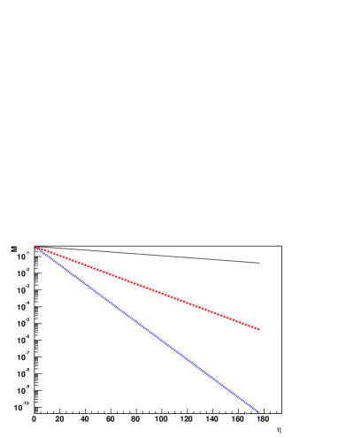
In Fig 1 we plot the relative change of the adiabatic invariant () for a particular Fourier mode (k=2) for different values for the coefficient . In practice, we fixed the value of and changed . In Fig 1 a we show, the change of M for different choice of parameters. In Fig 1 b we show the change of I. Even though the mass changes by orders of magnitude, our numerically calculated adiabatic invariant remains constant on the level of 0.01 %. Even for the values of the total change of the adiabatic invariant in the time considered (20 ) is very small.
2.4 The wave amplitude and the observed spectrum
The spectrum of particles produced by hydrodynamical velocity and pressure fields is determined at the freeze out. The standard way to calculate it is the Cooper-Fry prescription, and we discuss how it works in the case we discussed, with cosmological-style expansion. Although it is not identical to experimental conditions, with flow fields depending on spatial coordinates, one can still get some lesson from this example.
The simplest way to obtain a particle spectrum from the hydro calculation is to consider that the system behaves hydrodynamically till some freeze out happens and after that particles (created through a thermal distribution) free stream. If the case of flat space, when the spectrum is calculated though the Cooper-Fry prescription at some time, the free streaming stage does not change the invariant spectrum.
However this is not the case in our curved expanding space because particle momenta continue to change in the expanding Robertson Walker space (as an illustration, the cosmic microwave background has a Boltzmann distribution, but the temperature of the distribution is time dependent). Thus, if we would keep the radius of our “universe” to expand for ever, the spectrum of particles we calculate after freeze out will continuously change, dropping the measured temperature.
In order to obtain an answer that resembles more the experimental conditions one may consider the “universe” which stops expanding after the freezeout. Thus, the spectrum remains constant when the particles fly out of the collision region. As in [9] we will consider fixed proper time freezeout, for which
| (34) |
Where is the value of the universe size at freeze out (and constant afterwords as an assumption). This factor has to be included to get the correct dimensions. The exponent of the thermal distribution also includes such factor. For a small perturbation, it will be
| (35) |
From here we observe that for a fixed momentum () the relevant quantity that sets the correlations in the spectrum is . We have shown already that this combination of fields increases with time. Thus, the effect of a small disturbance at early times, when the medium is more dense, increase as the system expands and becomes more dilute, as the amplitude of the relevant hydrodynamic field grows.
3 Vanishing speed of sound and reflected waves
As stated in the introduction, the speed of sound reaches a minimum in the mixed phase. If the system experiences the first order phase transition, the speed of sound in the mixed phase should vanish, because the pressure does not change during this stage while the energy density does. In this section we study the consequences of a vanishing speed of sound for the sound propagation.
Let us start by noting that when the speed of sound vanishes, the adiabatic approximation explored in the previous section can no longer be applied. In fact, in such a case, the logarithmic derivatives of diverges and thus, (21) does not hold. Thus, we will need to solve numerically the equations (13) with the procedure checked in the previous section in order to investigate this effect.
In order to get somewhat realistic estimates of the effects, we will model both the expansion rate and the speed of sound according to the physical situation at RHIC. Inspired in the boost invariant scenario, we will chose R(t) such that the entropy density behaves as:
| (36) |
Where and . The value of will be specified later.
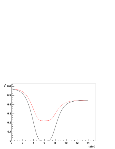
We now discuss the function . Numerical solutions of hydrodynamics as in [23] use values of the speed of sound that are discontinuous at the beginning of the three phases. Here, however, we study parametrization of the speed of sound that interpolate smoothly between the three stages of matter at RHIC. The times for the interpolation are also inspired in hydrodynamic solutions for RHIC [23]. Following these calculations we will assume that each of the three stages have the same time duration of 4 fm. Finally, in order to investigate the effect of the first order phase transition on the sound waves, we will leave the minimum value of the speed of sound in the mixed phase as a free parameter and we study the propagation of the waves for different values of this minimum. (see Fig. 2 a) ). Once the function is determined, we can solve (26) to obtain the temperature, imposing that at the time where has a minimum ( fm in our case) . This determines uniquely the temperature, and in particular the value . We use this value of the temperature and the equation of state for an ideal QGP in order to determine .
Once all the parameters are specified, we proceed to numerically solve (13). We will study the propagation of a spherical wave started from a perturbation at time t=0. Let us start our discussion with the case of vanishing minimum (first order phase transition). In this case, the spherical wave will split into two at the mixed phase, one propagating outwards (transmitted wave) and the second inwards (reflected) towards the origin. A simple physical explanation of this effect is as follows: when the speed of sound vanishes, all the information about the directionality of the wave disappears and, thus, when the speed of sound changes again to a finite value the disturbance splits into two, as it can propagate both inwards and outwards. Finally, the spherical wave propagating inwards eventually bounces back when it arrives at the origin, leading to a second outward moving spherical wave. This is observed in numerical solution as a double peaked structure of the spherical wave profile at sufficient late times.
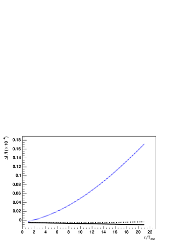
The appearance of the reflected wave happens not only when the speed of sound vanishes. We studied the spherical wave profile for different values of the minimum. This is best done at sufficiently late time, when the two waves (transmitted and reflected) propagate in the same direction. To illustrate the importance of the reflected wave, we study the amplitudes of the maximums in the wave profile for both waves at a late time. (In order to get rid of a trivial decay of the wave, we multiply them by the position of the maximum r.) Thus we define the relative amplitude:
| (37) |
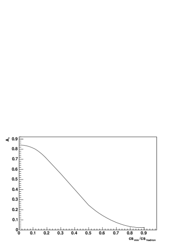
where the values are to be taken at the maxima of the disturbances. We plot this quantity in Fig 2 b). We observe that, as claimed, the reflected wave appears for non vanishing values of the minimal speed of sound. However the relative importance of the reflected wave decreases as the minimal value increases (as expected)
Even though the particular dependence of the relative amplitude with the minimal speed of sound, depends on our assumed parametrization , the general phenomenon is independent of the parametrization. As long as the speed of sounds vanishes at the mixed phase, we will obtain a reflected wave for the spherical disturbance.
Finally, for the cases where the minimal speed of sound does not vanish (as in the dashed curved in Fig.2 a ), we can use the adiabatic invariant to learn about the amplitude dependence of the disturbance. As we have specified a particular time dependence of and , we can complete the analysis of the previous section for this particular case. By solving (15) we find that for our parametrization of the speed of sound with minimum ranging from to , the effect of the overall dropping speed of sound increases the ratio by 10%. As before, the expansion of the medium also induces an amplitude increase. For our particular expansion rate, setting the freeze out time to , we obtain for the same quantity a factor of 3 increase (as the system becomes three times larger). These changes are very important experimentally, as the ratio enters in the exponent of the Cooper-Fry formula for the observed spectra.
3.1 Comparison to experimental correlation functions
Now we discuss where such reflected waves, if produced, will be located in the conical flow induced by high energy jets. The cone arises from the superposition of spherical waves produced along the path of the jet in the medium. All those disturbances produced prior to the mixed phase will encounter a time of minimum speed of sound. Following our previous discussion, if this minimum is small enough, all those waves will split into transmitted and reflected waves. After the superposition, given sufficient time, the reflected waves will generate a second cone. So, provided the observation time is late enough as for all the reflected wave to bounce back, one would find two cones with different opening angle propagating in the same direction.
However if the observation time is too close to emission time, one would find the the second cone moving inwards (or opposite direction to the jet). At RHIC the timing of the expansion is such that the three main stages – the QGP, the mixed phase and the hadronic phase – take roughly comparable period of proper time, about 4-5 fm/c each. The speed of sound at the QGP phase is larger than that in the final hadronic phase . Therefore, the distance the conical wave would propagate in QGP is larger than that in hadronic phase, and thus the reflected wave possibly reach the origin (for spherical wave, the original axes for conical one).
What this conclusion implies experimentally, is that the QCD phase transition is first order and the original wave gets split into direct and reflected waves, the freezeout will find the reflected wave on its way the origin, the opposite to the Mach direction of the direct wave. In terms of two particle azimuthal distribution it means the appearance of a second peak for . Even though detailed numerical simulations are needed to give the correct position of the peak, we give here a simple estimate for its location, based on geometrical optics.
The disturbance generated at the origin travels a distance AB
| (38) |
before the minimum of is reached and the wave splits into two. During the mixed phase the disturbance does not propagate, but after the hadronic stage starts, the waves propagates backwards a distance
| (39) |
Where is the freeze out time and we have assumed that the mixed QGP phase and the mixed phase have the same time duration. Thus, the relevant distance traveled by the wave is AC=AB-BC. The relevant longitudinal distance is not the distance traveled by the jet, but the distance traveled till the minimum of , (as after that time there is not more “emission” of reflected waves). Thus, the effective angle of emission is
| (40) |
where we used for AB and BC fixed values of and respectively.
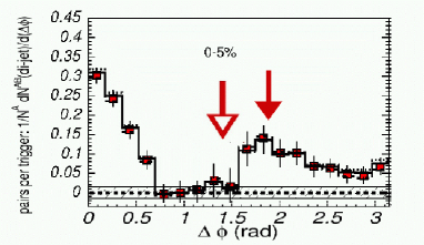
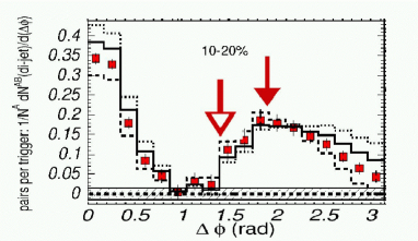
In Fig. 3 we show samples of experimental correlation function as obtained by PHENIX [18]. The peak around 1.9 rad (indicated by the filled arrow) corresponds to the Mach direction; this is the main effect attributed to a conical flow. The reflected wave should appear in the region , and the empty arrow shows the estimated place where the corresponding reflected peak should appear. Fig 3 a) shows the most central collisions, does not show any nonzero signal at that angle. Fig 3 b), at higher centrality, has a nonzero correlation function there, but it seems likely to be just a slope of a much broader peak.
We thus argue that there are no indications for enhanced correlations at the expected angle of the reflected wave, and thus the deconfining phase transition cannot be of the first order.
4 Summary and discussion
In this paper we have studied the effect of a variable speed of sound in the propagation of sound waves. We have considered for simplicity an expanding Universe with a flat Robertson-Walker metric, that allows us to introduce dynamical expansion depending on proper time only.
We have use the adiabatic approximation to investigate the effect of the expansion on the waves, concluding that even though the velocity field decreases with the expansion, the ratio of the velocity to the temperature increases. This ratio enters the exponent of the Cooper-Fry formula, and thus the observed effects in particle spectra may be significantly enhanced, the more so the larger is the particle momenta. We have shown that within the model studied based on the Robertson-Walker metric we obtain a 10 % increase of the ratio due to the change of and a factor 3 increase of this ratio due to the expansion. Even though this values depend on the particular model studied we expect a similar effect to take place in fireball expansion.
We have also studied the effect of a vanishing speed of sound, where the adiabatic approximation cannot be used. This is supposed to happen in the mixed phase the phase transition in QCD is first order. We have shown that this must lead to the appearance of reflected waves, the superposition of which leads to a second cone in the flow field. Given the timing of the different stages at RHIC the second cone should be moving inwards at the time of freezeout. We concluded that the first order phase transition should lead to a peak at a relative angle . The experimental correlation functions do not show any enhancement at this direction, which we think indicates that the phase transition in QCD cannot be of the first order. Needless to say, more theoretical and experimental work is needed before finalizing this important conclusion.
This work was partially supported by the Department of Energy (U.S.A.) under grants DE-FG02-88ER40388 and DE-FG03-97ER4014.
References
- [1] Adcox K et al (PHENIX) 2002 Phys. Rev. Lett. 88 022301 \nonumAdler C et al (STAR) 2002 Phys. Rev. Lett. 89 202301 \nonumAdler S S et al (PHENIX) 2003 Phys. Rev. Lett. 91 072301 \nonumAdams J et al (STAR) 2003 Phys. Rev. Lett. 91, 172302
- [2] Bjorken J D , FERMILAB-PUB-82-059-THY \nonumAppel D A 1986 Phys. Rev. D 33 717 \nonumBlaizot J P and McLerran L D 1986 Phys. Rev. D 34 2739
- [3] Gyulassy M and Plumer M 1990 Phys. Lett. B 243 432 \nonumWang X N, Gyulassy M and Plumer M, 1995 Phys. Rev. D 51 3436 \nonumFai G, Barnafoldi G G, M. Gyulassy, Levai P, Papp G, Vitev I and Zhang Y 2001 Preprint hep-ph/0111211
- [4] Baier R, Dokshitzer Y L, Peigne S and Schiff D 1995 Phys. Lett. B 345 277 \nonumBaier R, Dokshitzer Y L, Mueller A H and Schiff D 2001 JHEP 0109 033
- [5] Shuryak E V and Zahed I 2004 Preprint hep-ph/0406100
- [6] Wang X N, 2004 Preprint nucl-th/0405017
- [7] E. Shuryak, “Why does the quark gluon plasma at RHIC behave as a nearly ideal fluid?,” Prog. Part. Nucl. Phys. 53, 273 (2004) [arXiv:hep-ph/0312227].
- [8] Teaney D 2003 Phys.Rev. C 68 034913
- [9] J. Casalderrey-Solana, E. V. Shuryak and D. Teaney, arXiv:hep-ph/0411315. To be published in Journal of Physics G: in Proccedings of Workshop on Correlations and Fluctuations in Relativistic Nuclear Collisions, MIT, April 21-23, 2005
- [10] Stocker H 2004, nucl-th/0406018
- [11] L. M. Satarov, H. Stoecker, I. N. Mishustin, Phys. Lett. B 627 64,2005
- [12] T. Renk, J. Ruppert, hep-ph/0509036
- [13] J. Ruppert and B. Muller, Phys. Lett. B 618 123,2005
- [14] I. M. Dremin, hep-ph/0507167
- [15] V. Koch, A. Majumder, X. N. Wang, nucl-th/0507063
- [16] I. Vitev, hep-ph/0501255
- [17] Fuqiang Wang for STAR collaboration, (Quark Matter 2004), J.Phys.G 30 S1299-S1304,2004; Preprint nucl-ex/0404010, also Proceedings of the MIT workshop 2005.
- [18] Modifications to di-jet hadron pair correlations in Au+Au collisions at S(NN)**(1/2) = 200-GEV. PHENIX coll, nucl-ex/0507032, submitted to PRL; B.Jacak (for PHENIX), Int.conf. on Physics and Astropysics of QGP, Calcutta 2005,nucl-ex/0508036 ; B.Cole, Quark Matter 05, August 2005
- [19] C. M. Hung and E. V. Shuryak, Phys. Rev. C 57, 1891 (1998) [arXiv:hep-ph/9709264].
- [20] L. D. Landau, E. M. Lifshitz, Mechanics, Pergamon Press, 1976
- [21] Weinberg S, Gravitation and cosmology: principles and applications of the general theory of relativity. New York, Wiley (1972)
- [22] J. D. Anderson, Computational Fluid Dynamics, McGraw-Hill Inc. (1995)
- [23] D. Teaney, J Lauret, E. V. Shuryak, arXiv:nucl-th/0110037