Study of W-exchange Mode $D^{0}\to\phi\overline{K}^{0}$

Abstract

We calculate the branching ratio of rare decay $D^{0}\to\phi\overline{K}^{0}$ using the perturbative QCD factorization approach based on $k_{T}$ factorization. Our result shows this branching ratio is $(8.7\pm 1.4)\times 10^{-3}$, which is consistent with experimental data. We hope the CLEO-C and BES-III can measure it more accurately, which will help us understand QCD dynamics and $D$ meson weak decays.

The precise estimation of the branching ratio for the hadronic $D$ decays is very important both in theoretical side and experimental side. As a rare decay, $D^{0}\to\phi\overline{K}^{0}$ plays an important role in testing QCD dynamics and searching for new physics. In the standard model picture, this decay mode is a pure annihilation type decay, also called $W$-exchange mode. It has been discussed with a large branching ratio to explain the big difference of lifetime between $D^{0}$ and $D^{+}$ bigi . In the $80$’s of last century, this decay’s branching ratio has been measured in CLEO benek . With the development of experiments, this branching ratio is confirmed as pdg :

$$\mathrm{Br}(D^{0}\to\phi\overline{K}^{0})=(9.4\pm{1.1})\times 10^{-3}.$$ (1)

To our knowledge, this decay mode is never calculated quantitatively in QCD. So, it is necessary for us to reanalyze this decay mode seriously.

Based on the factorization hypothesis, many $D$ decays have been calculated in naive factorization approach BSW and QCD factorization approach QCDF . However, Annihilation diagrams can not be calculated easily for its endpoint singularity. It is well known that perturbative QCD (PQCD) factorization approach is successful in calculating two-body $B$ meson decays pqcd . The end point singularity can be regulated by Sudakov form factor and threshold resummation through introducing the transverse momentum $k_{T}$ of valence quarks. Thus, PQCD approach can give converging results and have predictive power. Using this approach, people have calculated many $B$ meson pure annihilation type decays quantificationally, and the results agree with data well lu:bdsk .

In this paper, we will calculate the $D^{0}\to\phi\overline{K}^{0}$ decay in PQCD approach. In this decay, the $W$ boson exchange induces the four quark operator $\bar{s}c\to\bar{u}d$, and the $\bar{s}s$ quarks included in $\phi,\overline{K}^{0}$ are produced from a gluon. This gluon can attach to any one of the quarks participating in the four-quark operator. In the rest frame of $D$ meson, the produced $s$ and $\bar{s}$ quark included in final states have momenta of $\mathcal{O}(P_{K}/2)$ and $\mathcal{O}(P_{\phi}/2)$, respectively. Therefore the gluon producing them has momentum $q\sim\mathcal{O}(M_{D}/2)$, which is nearly $1$ GeV. This hard gluon can be treated perturbatively. Therefore the hard part calculation involves not only the four quark operator but also the hard gluon connecting $s\bar{s}$ quark pair. The factorization here means the six quark hard part calculation factorize from the non-perturbative hadronization characterized by meson light cone wave functions.

We work at the $D$ meson rest frame for simplicity. In light-cone coordinate system, the momentum of the $D$, $\phi$ and $\overline{K}^{0}$ meson can be written as:

$$P_{1}=P_{D}=\frac{M_{D}}{\sqrt{2}}~{}(1,1,\vec{0}_{\perp}),P_{2}=P_{\phi}=\frac{M_{D}}{\sqrt{2}}~{}(1,r^{2},\vec{0}_{\perp}),P_{3}=P_{\overline{K}^{0}}=\frac{M_{D}}{\sqrt{2}}~{}(0,1-r^{2},\vec{0}_{\perp}),$$ (2)

where $r=M_{\phi}/M_{D}$ and we neglect the $\overline{K}^{0}$ meson mass $M_{\overline{K}^{0}}$ compared with the large $D$ meson mass. Because this decay is $D\to PV$ mode, the transverse polarization of $\phi$ meson gives no contribution. The longitudinal polarization vector of $\phi$ meson is given as:

$$\epsilon_{2L}=\frac{M_{D}}{\sqrt{2}M_{\phi}}~{}(1,-r^{2},\vec{0}_{\perp}).$$ (3)

Denoting the light (anti-)quark momenta in $D$, $\phi$ and $\overline{K}^{0}$ mesons as $k_{1}$, $k_{2}$, and $k_{3}$, respectively, we can choose

$$k_{1}=(x_{1}P_{1}^{+},0,{\bf k}_{1T}),\ k_{2}=(x_{2}P_{2}^{+},0,{\bf k}_{2T}),k_{3}=(0,x_{3}P_{3}^{-},{\bf k}_{3T}).$$ (4)

Then, integrating over $k_{1}^{-}$, $k_{2}^{-}$, and $k_{3}^{+}$, we get the decay amplitude:

$$\mbox{Amplitude}\sim\int\!\!dx_{1}dx_{2}dx_{3}b_{1}db_{1}b_{2}db_{2}b_{3}db_{3}\\ \mathrm{Tr}\bigl{[}C(t)\Phi_{D}(x_{1},b_{1})\Phi_{\phi}(x_{2},b_{2},\epsilon)\Phi_{K}(x_{3},b_{3})H(x_{i},b_{i},\epsilon,t)S_{t}(x_{i})\,e^{-S(t)}\bigr{]},$$ (5)

where $b_{i}$ is the conjugate space coordinate of ${\bf k}_{iT}$, and $t$ is the largest energy scale in $H$, as the function in terms of $x_{i}$ and $b_{i}$. The large logarithms ($\ln m_{W}/t$) coming from QCD radiative corrections to four quark operators are included in the Wilson coefficients $C(t)$. The large double logarithms ($\ln^{2}x_{i}$) on the longitudinal direction are summed by the threshold resummation, and they lead to a jet function $S_{t}(x_{i})$ which smears the end-point singularities on $x_{i}$. The last term, $e^{-S(t)}$, contains two kinds of logarithms. One of the large logarithms is due to the renormalization of ultra-violet divergence $\ln tb$, the other is resummation of double logarithm $\ln^{2}b$ from the overlap of collinear and soft gluon corrections. This Sudakov form factor suppresses the soft dynamics effectively. Thus it makes perturbative calculation of the hard part $H$ reliable. $\Phi_{M}$ is the wave function which describes the inner information of meson $M$.

For this decay, the relevant weak Hamiltonian is Buchalla:1996vs :

$$H_{\mathrm{eff}}=\frac{G_{F}}{\sqrt{2}}V_{cs}V_{ud}^{*}\left[C_{1}(\mu)O_{1}(\mu)+C_{2}(\mu)O_{2}(\mu)\right],$$ (6)

where $C_{i}(\mu)(i=1,2)$ is the QCD corrected Wilson coefficient at the renormalization scale $\mu$ and the four quark operators $O_{1}$ and $O_{2}$ are

$$O_{1}=(\bar{s}_{i}d_{i})_{V-A}(\bar{u}_{j}c_{j})_{V-A},O_{2}=(\bar{s}_{i}c_{i})_{V-A}(\bar{u}_{j}d_{j})_{V-A}.$$ (7)

The four lowest order Feynman diagrams of $D^{0}\to\phi\overline{K}^{0}$ in PQCD approach are drawn in FIG.1 according to this effective Hamiltonian.

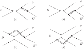
Figure 1: Leading order Feynman diagrams of $D^{0}\to\phi\overline{K}^{0}$

By calculating the hard part $H$ at the first order of $\alpha_{s}$, we get the following analytic formulas. With the meson wave functions, the amplitude for the factorizable annihilation diagrams in Fig.1(a) and (b) results in $F_{a}$ as:

$$F_{a}=-16\pi C_{F}M_{D}^{2}\int_{0}^{1}\!\!dx_{2}dx_{3}\int_{0}^{\infty}\!\!b_{2}db_{2}\,b_{3}db_{3}\times\Bigl{[}E_{f}(t_{a}^{1})h_{1}(x_{2},x_{3},b_{2},b_{3})\bigl{\{}(x_{3}-1)\phi_{\phi}(x_{2})\phi_{K}^{A}(x_{3})\\ -2r(x_{3}-2)r_{K}\phi_{\phi}^{s}(x_{2})\phi_{K}^{P}(x_{3})-2x_{3}rr_{K}\phi_{\phi}^{s}(x_{2})\phi_{K}^{T}(x_{3})\bigr{\}}-\bigl{\{}(x_{2}-1)\phi_{\phi}(x_{2})\phi_{K}^{A}(x_{3})\\ +2x_{2}rr_{K}\phi_{\phi}(x_{2})\phi_{K}^{P}(x_{3})-2r(x_{2}-2)r_{K}\phi_{\phi}(x_{2})\phi_{K}^{P}(x_{3})\bigr{\}}E_{f}(t_{a}^{2})h_{2}(x_{2},x_{3},b_{2},b_{3})\Bigr{]}.$$ (8)

In the function, $C_{F}=4/3$ is the group factor of $\mathrm{SU}(3)_{c}$, and $r_{K}=m_{0K}/M_{D}$, with $m_{0K}=m_{K}^{2}/m_{s}$ ($m_{s}$ is the $s$ quark current mass). The functions $E_{f}$ is :

$$E_{f}(t)=(C_{1}(t)+C_{2}(t)/3)\alpha_{s}(t)\ e^{-S_{\phi}(t)-S_{K}(t)}.$$ (9)

The hard scale $t$’s in the amplitudes are taken as the largest energy scale in the hard part $H$ in order to kill the large logarithmic radiative corrections:

$$t_{a}^{1}=\mathrm{max}(M_{D}\sqrt{1-x_{3}+x_{3}r^{2}},\frac{1}{b_{2}},\frac{1}{b_{3}}),t_{a}^{2}=\mathrm{max}(M_{D}\sqrt{1-x_{2}},\frac{1}{b_{2}},\frac{1}{b_{3}}).$$ (10)

The functions $h_{i}(i=1,2)$ in the decay amplitudes consist of two parts: one is the jet function $S_{t}(x_{i})$ derived by the threshold resummation, the other is the Fourier transformation of the propagator of virtual quark and gluon. They are given as:

$$h_{1}(x_{2},x_{3},b_{2},b_{3})=S_{t}(1-x_{3})\left(\frac{\pi i}{2}\right)^{2}H_{0}^{(1)}(M_{D}\sqrt{(1-x_{2})(1-x_{3}+x_{3}r^{2})}\,b_{2})$$

$$\times\left\{H_{0}^{(1)}(M_{D}\sqrt{1-x_{3}+x_{3}r^{2}}\,b_{2})J_{0}(M_{D}\sqrt{1-x_{3}+x_{3}r^{2}}\,b_{3})\theta(b_{2}-b_{3})+(b_{2}\leftrightarrow b_{3})\right\},$$ (11)

$$h_{2}(x_{2},x_{3},b_{2},b_{3})=S_{t}(1-x_{2})\left(\frac{\pi i}{2}\right)^{2}H_{0}^{(1)}(M_{D}\sqrt{(1-x_{2})(1-x_{3}+x_{3}r^{2})}\,b_{2})$$

$$\times\left\{H_{0}^{(1)}(M_{D}\sqrt{1-x_{2}}\,b_{2})J_{0}(M_{D}\sqrt{1-x_{2}}\,b_{3})\theta(b_{2}-b_{3})+(b_{2}\leftrightarrow b_{3})\right\}.$$ (12)

The amplitude for the nonfactorizable annihilation diagrams in Fig.1(c) and (d) results in

$$M_{a}=\frac{1}{\sqrt{2N_{c}}}64\pi C_{F}M_{D}^{2}\int_{0}^{1}\!\!dx_{1}dx_{2}dx_{3}\int_{0}^{\infty}\!\!b_{1}db_{1}\,b_{2}db_{2}\ \phi_{D}(x_{1},b_{1})\\ \times\Bigl{[}\bigl{\{}\left(x_{3}-1\right)\phi_{\phi}(x_{2})\phi_{K}^{A}(x_{3})-r\left(x_{2}+x_{3}-2\right)r_{K}\phi_{\phi}^{s}(x_{2})\phi_{K}^{P}(x_{3})-r\left(x_{2}-x_{3}\right)r_{K}\phi_{\phi}^{t}(x_{2})\phi_{K}^{P}(x_{3})\\ -r\left(x_{2}+x_{3}-2\right)r_{K}\phi_{\phi}^{t}(x_{2})\phi_{K}^{T}(x_{3})-r\left(x_{2}-x_{3}\right)r_{K}\phi_{\phi}^{s}(x_{2})\phi_{K}^{T}(x_{3})\bigr{\}}E_{m}(t_{m}^{1})h_{a}^{(1)}(x_{1},x_{2},x_{3},b_{1},b_{2})\\ -\bigl{\{}\left(x_{2}-1\right)\phi_{\phi}(x_{2})\phi_{K}^{A}(x_{3})-r\left(x_{2}+x_{3}-4\right)r_{K}\phi_{\phi}^{s}(x_{2})\phi_{K}^{P}(x_{3})-r\left(-x_{2}+x_{3}\right)r_{K}\phi_{\phi}^{t}(x_{2})\phi_{K}^{P}(x_{3})\\ -r\left(x_{2}-x_{3}\right)r_{K}\phi_{\phi}^{s}(x_{2})\phi_{K}^{T}(x_{3})+r\left(x_{2}+x_{3}\right)r_{K}\phi_{\phi}^{t}(x_{2})\phi_{K}^{T}(x_{3})\bigr{\}}E_{m}(t_{m}^{2})h_{a}^{(2)}(x_{1},x_{2},x_{3},b_{1},b_{2})\Bigr{]},$$ (13)

where $x_{1}$ dependence in the numerators of the hard part are neglected by the assumption $x_{1}\ll x_{2},x_{3}$. In the above Equation, some functions are defined as:

$$E_{m}(t) = C_{2}(t)\alpha_{s}(t)\,e^{-S_{D}(t)-S_{\phi}(t)-S_{K}(t)};$$ (14)

$$t_{m}^{j} = \mathrm{max}(M_{D}\sqrt{|F^{2}_{(j)}|},M_{D}\sqrt{(1-x_{2})(1-x_{3}+x_{3}r^{2})},\frac{1}{b_{1}},\frac{1}{b_{2}});$$ (15)

$$h^{(j)}_{a}(x_{1},x_{2},x_{3},b_{1},b_{2})=$$

$$\biggl{\{}\frac{\pi i}{2}\mathrm{H}_{0}^{(1)}(M_{D}\sqrt{(1-x_{2})(1-x_{3}+x_{3}r^{2})}\,b_{1})\mathrm{J}_{0}(M_{D}\sqrt{(1-x_{2})(1-x_{3}+x_{3}r^{2})}\,b_{2})\theta(b_{1}-b_{2})$$

$$\qquad\qquad\qquad\qquad+(b_{1}\leftrightarrow b_{2})\biggr{\}}\times\left(\begin{matrix}\mathrm{K}_{0}(M_{D}F_{(j)}b_{1}),&\text{for}\quad F^{2}_{(j)}>0\\ \frac{\pi i}{2}\mathrm{H}_{0}^{(1)}(M_{D}\sqrt{|F^{2}_{(j)}|}\ b_{1}),&\text{for}\quad F^{2}_{(j)}<0\end{matrix}\right),$$ (16)

with:

$$F^{2}_{(1)}=(-x_{1}+x_{2}+1)(1-x_{3}+x_{3}r^{2}),F^{2}_{(2)}=x_{3}(x_{2}-x_{1})(1-r^{2})-1.$$ (17)

The total decay amplitude for $D^{0}\to\phi\overline{K}^{0}$ decay is given as $A=f_{D}F_{a}+M_{a}$. The decay width is then

$$\Gamma(D^{0}\to\phi\overline{K}^{0})=\frac{G_{F}^{2}M_{D}^{3}}{128\pi}(1-r^{2})|V_{ud}^{*}V_{cs}A|^{2}.$$ (18)

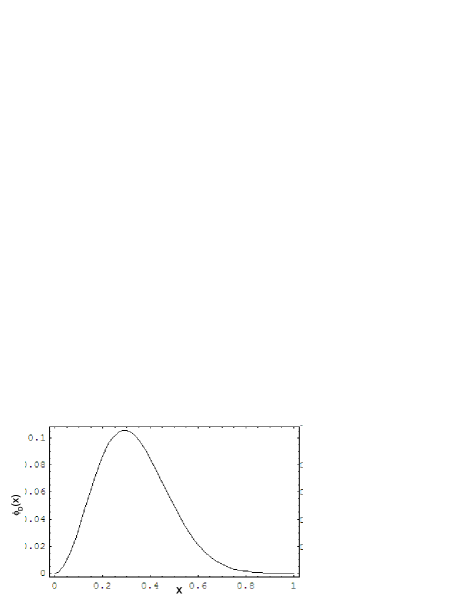
Figure 2: The $D$ meson distribution amplitude

For numerical analysis, we use the following input parameters pdg :

$$f_{D}=230\mbox{ MeV},~{}f_{K}=160\mbox{ MeV},~{}f_{\phi}=241\mbox{ MeV},m_{0K}=1.7\mbox{ GeV},$$

$$|V_{ud}|=0.9734,~{}|V_{cs}|=0.974,\tau_{D^{0}}=4.1\times 10^{-13}\mbox{s},~{}f_{\phi}^{T}=220\mbox{MeV}.$$ (19)

The branching ratio obtained from the analytic formulas may be sensitive to many parameters especially those in the meson wave functions. The light $\phi$ and $K$ mesons’ distribution amplitudes up to twist-3 have been used for many times in $B$ decays pqcd , and we don’t list them here. The meson ($\phi$, $K$) wave functions are well constrained by hadronic $B$ decays experiments.

However, the heavy meson wave functions are still in discussion especially for $D$ meson. In this work, the $D$ meson distribution amplitude we used has only one parameter $\omega_{D}$, which is similar to $B$ meson pqcd :

$$\phi_{D}(x,b)=Nx^{2}(1-x)^{2}\exp\left[-\frac{M_{D}^{2}\ x^{2}}{2\omega_{D}^{2}}-\frac{1}{2}(\omega_{D}b)^{2}\right],$$ (20)

where $N$ is a normalization factor. For $B$ meson, the peak appears at $x=0.1$, because $b$ quark is much heavier than the light $d$ quark. For $D$ meson, the ratio of heavy $(c)$ and light quark $(u)$ mass is rather smaller than that of $B$ meson. So we adjust the parameter $\omega_{D}=0.5\mbox{ GeV}$, which makes the distribution amplitude peak at $x=0.3$. The shape of the $D$ meson distribution amplitude is shown in FIG.2. Using this wave function, we can get the form factor of $D\to K$ as $F^{D\to K}=0.80$. This result is consistent with the previous calculation $F^{D\to K}=0.78\pm 0.04$ formf . In fact, the heavy meson distribution amplitude can be eventually determined by radiative leptonic $D$ meson decayssong .

Here if we let $\omega_{D}$ vary from $0.45$ to $0.55$, the branching ratios of $D^{0}\to\phi\overline{K}^{0}$ decay is:

$$\mathrm{Br}(D^{0}\to\phi\overline{K}^{0})=(8.7\pm{1.6})\times 10^{-3},$$ (21)

which is consistent with the experimental measurement shown in eq.(1). From this calculation, we find that the branching ratio becomes large when $\omega_{D}$ arise. Many other parameters such as Chiral breaking scale $m_{0K}$, CKM matrix elements also have large uncertainties, which will also enlarge the theoretical uncertainties for branching ratios.

In general, if a process happens in an energy scale where there are many resonance states, this process must be seriously affected by these resonances. This is a highly non-perturbative strong interaction effect. Near the scale of $D$ meson mass many resonance states exist, which may give large pollution to $D$ decays calculation. So the final states interaction (FSI) may be important. However, we cannot calculate the FSI’s contribution from the first principle. Although many people have discussed final states interaction in $D$ decay FSI , there is large uncertainty in the calculation because they are usually model dependent. In our PQCD calculation we factorize the non-perturbative effects in meson wave functions, but neglect the soft FSI effect. Our numerical result is consistent with the experimental data well. It is a hint, that the contribution from soft FSI may not play an important role in this decay. We think the CLEO-C and BES can measure this $W$-change channel more accurately, which will afford help for us to understand the dynamics of $D$ decay. And the results also help us determine the $D$ meson distribution amplitude. Since there is only tree operators contributing to this decay (only one kind of weak phase), there is no direct $CP$ violation in the standard model. Any non-zero measurement of direct $CP$ in this decay will be a signal of new physics.

In a summary, we calculate the branching ratio of $D^{0}\to\phi\overline{K}^{0}$ in the perturbative QCD factorization approach without considering final states interaction. Our result indicates this branching ratio is very large comparing with other pure annihilation decay channels, because there is no Cabibbo suppression. This branching ratio is about $8.7\times 10^{-3}$, and has been measured by CLEO. We hope the CLEO-C and BES-III can measure it more accurately, which will help us test QCD dynamics.

References

(1) I. Bigi and M. Fukugita 1980 Phys. Lett. B91 121.
(2) C. Benek, et.al 1986 Phys. Rev. Lett56 1893.
(3) Particle Data Group, S. Eidelman, et al. 2004 Phys. Lett. B592 1.
(4)
M. Bauer and B. Stech 1985 Phys. Lett. B152 380;
M. Bauer, B. Stech and M. Wirbel 1987 Z. Phys. C34 103.
(5)
GONG H.-J, SUN J.-F and DU D.-S 2002 HEP and NP26 665;
LAI J.-H and YANG K.-C 2005 Phys.Rev. D72 096001.
(6)
Y.-Y. Keum, LI H.-N and A. I. Sanda 2001 Phys. Rev. D63 054008;
LÜ C.-D, K. Ukai and YANG M.-Z 2001 Phys. Rev. D63 074009.
(7)
LÜ C.-D. and K. Ukai 2003 Eure.Phy.J.C28, 305 (2003);
LI Y and LÜ C.-D, 2003 J. Phys. G29 2115-2124;
LÜ C.-D 2002 Eure.Phy.J.C24 121.
(8) G. Buchalla, A. J. Buras and
M. E. Lautenbacher, 1996 Rev. Mod. Phys68 1125.
(9)
S. V. Semenov 2003 Yad. Fiz66 [2003 Phys. At. Nucl66, 526 ].
(10) LÜ C-D and SONG G-L 2003 Phys. Lett.B562 75.
(11) H. J. Lipkin 1980 Phys. Rev. Lett44 710;
J. F.Donoghue, B. R.Holstein 1980 Phys. Rev. D21 1334;
M.Ablikim, DU D.-S and YANG M.-Z 2002 Phys. Lett. B536 34.