Constraining renormalon effects in lattice determination of heavy quark mass

Abstract

The Borel summation technique of infrared renormalons is applied to the lattice determination of heavy quark mass. With Borel summation a physical heavy quark pole mass and binding energy of a heavy-light meson can be defined in a rigorous and calculable manner. A notable feature of the Borel summation, compared to the usual perturbative cancellation of IR renormalons, is an automatic scale isolation. The two approaches of handling renormalon divergence are compared in the B-meson as well as in an (imaginary) heavy-light meson with a mass much larger than the inverse of the lattice spacing.

The lattice simulation of the heavy quark effective theory of QCD can provide potentially a most accurate determination of the bottom quark mass. Essential in the calculation is constraining the unknown higher order contributions in the perturbative matching of the lattice heavy quark effective theory and QCD. The matching relation for the heavy-quark mass reads  Crisafulli et al. (1995)

$$m_{\rm b}^{\rm pole}=M_{\rm B}-\bar{\Lambda}\,,\quad\bar{\Lambda}\equiv{\cal E}(a)-\delta m(a)\,,$$ (1)

where $\bar{\Lambda}$ denotes the renormalized binding energy, $a$ is the lattice spacing, $M_{\rm B}$ is the B-meson mass, $\delta m$ is the mass shift in the static limit, and ${\cal E}$ is the binding energy that is to be computed in lattice simulation. Here $1/m_{\rm b}$ corrections are ignored. The mass shift as well as the matching relation between the pole mass and $\overline{\rm MS}$ mass can be computed in perturbation theory, and with high order perturbative calculations of the matching relations an accurate determination of the $\overline{\rm MS}$ mass is possible from a precision calculation of ${\cal E}(a)$.

There is a caveat, however. As well known, the pole mass and mass shift suffer from renormalon divergences, and are not well-defined in perturbation theory. A well known approach for dealing this problem is to bypass the notion of pole mass (and any long-distance quantities) and deal directly with a short-distance mass, imposing renormalon cancellation perturbatively  Beneke and Braun (1994); Bigi et al. (1994); Martinelli and Sachrajda (1996). This idea, when applied to Eq.  (1), yields

$$m_{\rm b}^{\overline{\rm MS}}=\Delta(a)\left(1+\sum_{n=0}^{\infty}r_{n}(\mu/m_{\rm b}^{\overline{\rm MS}},\mu a)\alpha_{s}(\mu)^{n+1}\right)$$ (2)

where $m_{\rm b}^{\overline{\rm MS}}$ is the $\overline{\rm MS}$ mass satisfying $m_{\rm b}^{\overline{\rm MS}}=m_{\rm b}^{\overline{\rm MS}}(m_{\rm b}^{\overline{\rm MS}})$ and $\mu$ denotes the renormalization scale and $\Delta(a)\equiv M_{\rm B}-{\cal E}(a)$. The coefficients $r_{n}$, which can be obtained from the perturbative expansions of the pole mass and mass shift, do not suffer from the renormalon divergence, since the renormalon divergence in the pole mass is cancelled by that in the mass shift. Eq.  (2) truncated at next-leading order (NLO) was used in Ref.  Martinelli and Sachrajda (1999) in determining the $\overline{\rm MS}$ mass for the b-quark (A slightly different approach may also be found in Bali and Pineda (2004)). For the sake of convenience, we shall call this method of handling the renormalon divergence the perturbative cancellation method (PCM).

Let us now mention two characteristics of the PCM. We first notice that the coefficients $r_{n}$ depend on two independent scales, $m_{\rm b}^{\overline{\rm MS}}$ and $1/a$, through the renormalization scale. When the two scales are far separated, this can, in principle, delay the convergence of the expansion  (2) and be problematic with low order perturbations. This scale mixing is an unavoidable, generic problem as long as the renormalons in hard and soft quantities are cancelled in the perturbative way. Secondly, the PCM may not utilize the known perturbative expansions of the involved quantities to the fullest. Since $r_{n}$ is given by a linear combination of the perturbative coefficients of the pole mass and mass shift to the order $n$ the expansion  (2) can be determined only to the order where both quantities are known. For example, this prevented the PCM from using the next-next-leading order (NNLO) calculation of the pole mass before the NNLO calculation of the mass shift. Although the pole mass as well as mass shift are presently known to NNLO a future next-next-next-leading order calculation of one of these quantities cannot be utilized until both quantities are calculated to the same order. Our main point in this paper is that these undesirable features of the PCM can be solved through the Borel summation of the divergent series for the infrared-sensitive quantities.

A fundamentally different approach to the renormalon problem was proposed recently, in which the divergent perturbative expansions are Borel summed to all orders  Lee (2003a). As well known, an infrared (IR) renormalon caused large order behavior is of same sign and cannot be Borel summed. This means that the Borel summation is ambiguous, depending on the integration contour of the Borel integral.

This ambiguity of Borel summation, however, should not appear in physical observables, and this implies that the ambiguities in the Borel summation must cancel. In the case of the matching relation  (1), the renormalons in the pole mass and mass shift should cancel since $M_{\rm B}$ must be free from the renormalon ambiguity.

When the perturbative series of the pole mass or mass shift is Borel summed, with the positive real axis on the upper half-plane as the contour of the Borel integral, the ambiguity appears through the imaginary part of the Borel integral. This ambiguity is known to be proportional to $\Lambda_{\rm QCD}$ and independent of the renormalization scheme and scale of the perturbation expansion  Beneke (1995). Applying this Borel summation on the perturbative series for the pole mass as well as the mass shift in Eq.  (1) we can now write the matching relation as

$$m_{\rm b}^{\rm BR}=M_{\rm B}-\bar{\Lambda}^{\rm BR}\,,\quad\bar{\Lambda}^{\rm BR}\equiv{\cal E}(a)-\delta m^{\rm BR}(a)\,,$$ (3)

where the ‘BR’ quantities are defined as the real parts of the following Borel integrals,

$$m_{\rm b}^{\rm BR}=m_{\rm b}^{\overline{\rm MS}}\left(1+\frac{1}{\beta_{0}}{\rm Re}\int_{0+i\epsilon}^{\infty+i\epsilon}e^{-b/\beta_{0}\alpha_{s}(\mu)}\widetilde{\cal M}_{\rm b}(\mu/m_{\rm b}^{\overline{\rm MS}},b)\,db\right)\,,$$

$$\delta m^{\rm BR}(a)=\frac{1}{a\beta_{0}}{\rm Re}\int_{0+i\epsilon}^{\infty+i\epsilon}e^{-b/\beta_{0}\alpha_{s}(\mu)}\widetilde{\delta\cal M}(\mu a,b)\,db\,,$$ (4)

where ${\widetilde{\cal M}}_{\rm b}(\mu/m_{\rm b}^{\overline{\rm MS}},b)$ and $\widetilde{\delta{\cal M}}(\mu a,b)$ are the Borel transforms of ($m_{\rm b}^{\rm pole}/m_{\rm b}^{\overline{\rm MS}}-1$) and $a\delta m$, respectively, and $\beta_{0}$, the one loop coefficient of the QCD $\beta-$function, is inserted here for the normalization convenience of the Borel transforms. The respective imaginary parts of the above Borel integrals are identical, canceling each other on Eq.  (1), and so can be ignored altogether, leaving only the real parts in the matching relation. This means that, unlike the PCM where the renormalon cancellation is implemented order by order perturbatively, the renormalon cancellation in Borel summation is exact from the beginning. The importance of this will be further discussed in the following. Another nice feature of the Borel summation is that it preserves the original form of the matching relation, but unlike Eq.  (1), all involved quantities are now well-defined; Eq.  (1) becomes rigorous through the Borel summation.

The exact nature of renormalon cancellation of the Borel summation method has an important implication. It resolves the scale mixing problem of the PCM mentioned above and also allows one to utilize all the available perturbative expansions for the pole mass as well as the mass shift, since these two quantities are Borel summed independently of each other. Because $m_{\rm b}^{\rm BR}$ and $\delta m^{\rm BR}$ are renormalization group (RG) invariant, one can choose the renormalization scale, as well as even the scheme, for the pole mass independently of those for the mass shift. This is in stark contrast with the PCM where the same renormalization scheme and scale should be chosen for both the pole mass and mass shift to ensure renormalon cancellation. This flexibility in choosing the RG scheme and scale can be exploited to optimize the Borel summations, which we will demonstrate later on by choosing independent RG scales in Borel summing the pole mass and mass shift.

The Borel summed $m_{\rm b}^{\rm BR}$ can, naturally, be called a pole mass. By definition it has, when reexpanded in $\alpha_{s}(\mu)$, exactly the same perturbative expansions as the (perturbative) pole mass, so is not a short-distance mass, but nevertheless is a well-defined quantity. This is also true with $\delta m^{\rm BR}$, or $\bar{\Lambda}^{\rm BR}$. Also, $m_{\rm b}^{\rm BR}$ and $\bar{\Lambda}^{\rm BR}$ are independent of the RG scheme and scale as well as the lattice spacing $a$, so in this respect may be called ‘physical’, although it does not mean that the heavy-quark propagator, for instance, has a true pole at the BR mass. They are also defined system-independently, so once determined, can be used in any other systems. As has been shown in  Lee (2003a, b) and will be repeated here later on, the ratio $m_{\rm b}^{\rm BR}/m_{\rm b}^{\overline{\rm MS}}$ can be calculated very accurately with the known perturbative expansions of the pole mass. This means that the BR mass can be converted accurately to the $\overline{\rm MS}$ mass, and vice versa, and can be freely used wherever the use of a pole mass is more desirable.

Defining a pole mass or a binding energy, formally, through the Borel summation is well-known, but the difficulty, however, lies with the computability of thusly defined quantities; If the Borel integrals of those quantities cannot be computed, to within the necessary accuracy, using the available information on the Borel transforms the formal BR definitions alone would be useless. The essential problem thus is how to rebuild the Borel transforms sufficiently accurately, not only around the origin in the Borel plane, where the ordinary perturbation can be applied, but also about the renormalon singularity that causes the renormalon divergence. Clearly, because of the renormalon singularity, the usual perturbative expansions of the Borel transforms about the origin alone would not suffice.

Since the renormalon ambiguity is $O(\Lambda_{\rm QCD})$, to solve the renormalon problem it is necessary to calculate the BR quantities to an accuracy better than $O(\Lambda_{\rm QCD})$. This requires an accurate description of the Borel transforms in the region in the Borel plane that contains the origin as well as the first IR renormalon singularity, since the renormalon ambiguities arise from the closest singularity to the origin. With many orders of perturbative expansions, perhaps many tens as may be inferred from the solvable instanton models in quantum mechanics  Zinn-Justin (1989), and the help from analytic continuations this could, in principle, be achieved, but is not possible in QCD since only the first few perturbative terms are known. Without employing a very large number of perturbative expansions it is simply impossible to reconstruct the renormalon singularity using the perturbative Borel transforms. It is important to realize that this calculability problem, not the renormalon ambiguity, led to the abandonment of infrared-sensitive quantities such as the pole mass. We give in the following a brief account on how this calculability problem can be resolved by judiciously taking into account the known properties of the renormalon singularity in addition to the usual perturbative expansions.

In Refs.  Lee (2003a, b) we have shown that the above calculability problem can be resolved in the case of the pole mass and heavy quark potential using an interpolation technique of the Borel transform, which we call bilocal expansion. A good description of the Borel transform about the origin can be obtained from the first terms of perturbation, and the behavior of the Borel transform about the renormalon singularity can also be learned, except for the residue of the singularity that determines the overall normalization of the renormalon-caused large order behavior, from the RG invariance of the renormalon ambiguity  Beneke (1995). Once the residue is known, one can then interpolate the above two known behaviors to obtain an accurate description of the Borel transform in the region of interest in the Borel plane. Of course, for this program to work it is essential to calculate the renormalon residue, and this problem can be solved with the perturbation scheme for the residue calculation developed in Refs.  Lee (1997, 1999). Fortunately, this perturbative calculation of the residue for the pole mass turns out to converge very well, due to the overwhelming dominance of the first IR renormalon in the $\overline{\rm MS}$ scheme, and allows one to calculate the residue to within a few percent of errors  Lee (2003a); Pineda (2001).

The Borel transform in bilocal expansion has two indices that denote the orders of the expansions about the origin and the renormalon singularity. For instance, in the case of the pole mass, the Borel transform ${\widetilde{\cal M}}_{\rm b}(\mu/m_{\rm b}^{\overline{\rm MS}},b)$ is approximated by ${\widetilde{\cal M}}_{\rm b(M,N)}(\mu/m_{\rm b}^{\overline{\rm MS}},b)$ with the latter converging to the exact Borel transform in the $M,N\to\infty$ limit. The indices $M$ and $N$ corresponds to the order of perturbative expansions about the origin and about the renormalon singularity, respectively. With the perturbative calculations up to NNLO for the pole mass and the four loop $\beta$-function, with the latter controlling the expansion about the renormalon singularity, ${\widetilde{\cal M}}_{b(M,N)}$ can be obtained for any combinations of $(M,N)$ with $M=0,1,2$ and $N=1,2$. In the following we shall keep the bilocal expansions to the highest known order, presently $N=1$, for the expansions about the renormalon singularity, and consider expansions about the origin with $M=0,1,2$, calling them the leading order (LO), NLO, and NNLO, respectively. For the details of the bilocal expansion we refer the readers to Refs.  Lee (2003b, a).

This bilocal expansion was shown to be very effective in Borel summing the pole mass as well as static interquark potential  Lee (2003a). The Borel summed pole mass and interquark potential converge rapidly under the bilocal expansion, and the resummed interquark potential agrees remarkably well with the lattice potential up to the interquark distances as large as about 0.7 ${\rm GeV}^{-1}$ (See Pineda (2003); Recksiegel and Sumino (2003) for the PCM approach to the static potential). Other applications in heavy quark physics may be found in Refs.  Lee (2003c, b); Kim et al. (2004); Andersen and Gardi (2005, 2006).

Figure 1: $m_{\rm b}^{\rm BR}/m_{\rm b}^{\overline{\rm MS}}$ vs $\mu$. The dotted, dashed, and solid lines are from using the Borel transforms $\widetilde{\cal M}_{\rm b(0,2)},\widetilde{\cal M}_{\rm b(1,2)}$, and $\widetilde{\cal M}_{\rm b(2,2)}$, respectively.

Now, going back to Eqs. (4) we compute the Borel summed pole mass $m_{\rm b}^{\rm BR}$ as well as the mass shift $\delta m^{\rm BR}(a)$ using the bilocal expansion described above. For the mass shift we use the known first three terms of its perturbative expansion, which allows us to compute the Borel transform $\widetilde{\delta{\cal M}}_{(M,N)}(\mu a,b)$ for $M=0,1,2$ and $N=1,2$. With these Borel transforms computing the Borel integrals is then straightforward using a conformal mapping. For the details of the computation we refer the readers to Ref.  Lee (2003b) where the Borel summation of the pole mass is described in detail. The only difference with the present computations is that the Borel integrals in (4) are with respect to $\alpha_{s}(\mu)$, whereas in Ref.  Lee (2003b) it was with $\alpha_{s}(m_{\rm b}^{\overline{\rm MS}})$. With this change in the RG scale it is necessary to rescale the renormalon residues accordingly. The RG invariance of the renormalon ambiguity demands the renormalon residue scale linearly in $\mu$, which implies the residue (of the first IR renormalon singularity) of ${\widetilde{\cal M}}_{\rm b}(\mu/m_{\rm b}^{\overline{\rm MS}},b)$ is given by $\bar{C}\mu/m_{\rm b}^{\overline{\rm MS}}$ where $\bar{C}$ denotes the reside at the scale $\mu=m_{\rm b}^{\overline{\rm MS}}$, and the residue of $\widetilde{\delta{\cal M}}(\mu a,b)$ is $\bar{C}a\mu$. For the quenched case ($N_{f}=0$) the perturbative computation of the residue using the expansions of the pole mass up to NNLO gives

$$\bar{C}=0.424+0.168+0.035=0.627\,,$$ (5)

where each terms denote the LO, NLO, and NNLO contributions, respectively.

Throughout the paper we focus our attention only to the quenched QCD, since only the quenched lattice data for the binding energy are available, and our main purpose is not to determine the $\overline{\rm MS}$ mass as precisely as possible but to make a comparison of the two approaches for handling the renormalon divergence. Hence in the following computations we also do not attempt to make detailed error estimates other than those of perturbative origin.

The running coupling $\alpha_{s}(\mu)$ used in the following computations is obtained using the four loop $\beta$-function and the lattice determination of $\Lambda_{\rm QCD}$ in quenched limit  Capitani et al. (1999)

$$\Lambda_{\overline{\rm MS}}^{(0)}r_{0}=0.602\,,$$ (6)

where $r_{0}$ denotes the Sommer scale whose value is taken to be $1/r_{0}=0.395$ GeV.

First, we present the Borel summed pole mass in Fig. 1 as functions of the RG scale. Notice that the $m_{\rm b}^{\rm BR}$ at NNLO using the Borel transform $\widetilde{\cal M}_{\rm b(2,2)}$ has a very small scale dependence, especially below $\mu=m_{\rm b}^{\overline{\rm MS}}$, where the optimal scale is expected to be on. Putting $\mu=m_{\rm b}^{\overline{\rm MS}}$ and $m_{\rm b}^{\overline{\rm MS}}=4.31\,\,{\rm GeV}$, as an example, we get

$$\frac{m_{\rm b}^{\rm BR}}{m_{\rm b}^{\overline{\rm MS}}}=1+0.11810+0.00044-0.00051$$ (7)

with each terms denoting the contributions from the Borel transforms $\widetilde{\cal M}_{\rm b(0,2)},(\widetilde{\cal M}_{\rm b(1,2)}-\widetilde{\cal M}_{\rm b(0,2)})$, and $(\widetilde{\cal M}_{\rm b(2,2)}-\widetilde{\cal M}_{\rm b(1,2)})$, respectively. Notice that the bulk of the Borel summation is given by the LO contribution and the higher order terms in bilocal expansion add only small corrections. This indicates that the leading order Borel transform, with the renormalon singularity properly taken into account, already provides an excellent profile of the true Borel transform in the domain of interest in the Borel plane, with the higher order terms contributing only small modifications . The weak dependence on the RG scale as well as the small size of the last two terms show that the relation between the BR mass and $\overline{\rm MS}$ mass for the bottom quark can be precisely determined to within a few parts in $10^{4}$.

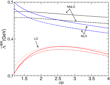
Figure 2: The Borel summed binding energy vs $\mu$. The dotted, dashed, and solid lines are at lattice spacings $a^{-1}=2.12,2.91,$ and $3.85$, respectively, using the leading order Borel transforms $\widetilde{\delta\cal M}_{(0,2)}$, NLO Borel transforms $\widetilde{\delta\cal M}_{(1,2)}$, and NNLO Borel transforms $\widetilde{\delta\cal M}_{(2,2)}$. Notice that the lines for $a^{-1}=2.12$ and 2.91 at NNLO (also at NLO) are almost on top of each other.

Now using the NLO and NNLO calculations for the mass shift Martinelli and Sachrajda (1999); Di Renzo and Scorzato (2001) we get the following bilocal Borel transform for the mass shift to NNLO as

$$\widetilde{\delta\cal M}_{(M,2)}(\xi,b) = \sum_{n=0}^{M}\frac{h_{n}(\xi)}{n!}\left(\frac{b}{\beta_{0}}\right)^{n}+\frac{\bar{C}\xi}{(1-2b)^{1+\nu}}\left[1+\sum_{i=1}^{2}c_{i}(1-2b)^{i}\right]\,,$$ (8)

where

$$h_{0} = 2.1173-\bar{C}\xi(1+c_{1}+c_{2})\,,$$

$$h_{1} = 3.7068\log(\xi)-1.3053-2\bar{C}\xi\beta_{0}[1-c_{2}+\nu(1+c_{1}+c_{2})]\,,$$

$$h_{2} = 6.4895\log(\xi)^{2}-1.8353\log(\xi)+9.6538-$$ (9)

$$4\bar{C}\xi\beta_{0}^{2}[2+\nu(3+c_{1}-c_{2})+\nu^{2}(1+c_{1}+c_{2})]\,,$$

where $\xi=a\mu$ and

$$\beta_{0}=\frac{11}{4\pi}\,,\quad\nu=\frac{51}{121}\,,\quad c_{1}=-0.2151\,,\quad c_{2}=0.1848\,.$$ (10)

The Borel summed binding energies vs $\mu$ from these Borel transforms are shown in Fig.   2 at lattice spacings $a^{-1}=2.12,2.91$, and $3.85$ GeV. Notice that $\mu$ is in units of the inverse lattice spacing that is the only scale relevant for the mass shift. This flexibility of choosing the RG scale independently of that of the pole mass is a clear advantage over the PCM. The binding energies ${\cal E}(a)$ used in this calculation were taken from the lattice data summarized in Ref.  Martinelli and Sachrajda (1999) which read

$$a{\cal E}(a)=0.61,\,0.52,\,0.46$$ (11)

at the lattice coupling $\beta=6.0,6.2,6.4$ that correspond to $a^{-1}=2.12,2.91$, and $3.85$ GeV, respectively. The lattice spacing from the lattice coupling was obtained following Capitani et al. (1999).

We first notice that the dependence on the RG scale of the Borel summed binding energy $\bar{\Lambda}^{\rm BR}$ at NNLO is less than $10\,{\rm MeV}$ over the range of $\mu$ shown ($1.2/a\leq\mu\leq 4/a$), and, remarkably, the binding energies at NLO and at NNLO for the two lattice spacings, $a^{-1}=2.12$ and 2.91, are virtually identical. On the other hand the binding energies for $a^{-1}=3.85$ are about 15 MeV larger than those of the other lattice spacings, which we suspect from the similarity of the line shapes at NNLO (also at NLO) should be largely due to the errors in ${\cal E}(a)$ from lattice simulation or in the relation between the lattice coupling and lattice spacing than in perturbation theory. We find the minimal sensitivity scales for the NNLO curves are at $\mu^{*}\approx 1.41/a$ for all the three values of the lattice spacing, which turns out to be close to the BLM scale that is about $1.45/a$  Martinelli and Sachrajda (1999). Also the differences about the optimal scale between the NLO and NNLO results are small. All these indicate that the perturbative uncertainty in the binding energy is well under control with the uncertainty being at most $\pm 10\,{\rm MeV}$.

Now reading the binding energies at the optimal scale we obtain

$$\bar{\Lambda}^{\rm BR}=0.458\,,0.458\,,0.474\,{\rm(GeV)}$$ (12)

at $1/a=2.12\,,2.91\,,3.85$ (GeV), respectively. Using these values and the physical B-meson mass $M_{\rm B}\!=\!5.279\,{\rm GeV}$ we get the corresponding BR masses from Eq.  (3)

$$m_{\rm b}^{\rm BR}=4.821\,,4.821\,,4.805\,{\rm(GeV)}\,$$ (13)

which have the same uncertainty as the binding energies in (12), ignoring the negligibly small experimental uncertainty in $M_{\rm B}$. Having the BR mass we can now obtain the $\overline{\rm MS}$ mass from the relation between the BR mass and $\overline{\rm MS}$, which is very similar to (7) but obtained using $\alpha_{s}(m_{\rm b}^{\overline{\rm MS}})$, with $m_{\rm b}^{\overline{\rm MS}}$ determined self-consistently. The result is summarized in Table   1. The uncertainties in the extracted $\overline{\rm MS}$ masses come entirely from the binding energies $\bar{\Lambda}^{\rm BR}$, since the conversion from the BR masses to $\overline{\rm MS}$ masses adds only a negligible error, about a few MeV. Thus the perturbative uncertainty in the $\overline{\rm MS}$ mass is also estimated to be $\pm 10\,{\rm MeV}$.

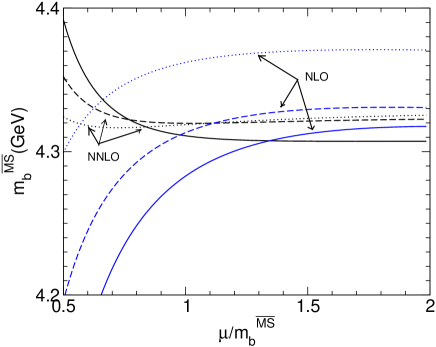
Figure 3: The RG scale dependence of $\overline{\rm MS}$ mass determined in the PCM. The dotted, dashed, and solid lines are at lattice spacings $a^{-1}=2.12,2.91,$ and $3.85$, respectively.

Let us now see the scale dependence of the $\overline{\rm MS}$ mass determined in the PCM based on Eq.  (2). From the NNLO calculations of the mass shift and pole mass the first three coefficients $r_{0},r_{1},r_{2}$ read

$$r_{0} = \frac{2.1173}{\Delta a}-0.4244\,,$$

$$r_{1} = \frac{1}{\Delta a}(3.7068\log(\xi)-2.2039)-1.1820-0.8488\beta_{0}\log(\chi)\,,$$

$$r_{2} = \frac{1}{\Delta a}[6.4894\log(\xi)^{2}-3.4084\log(\xi)+7.7051-1.7972\beta_{0}\log(\chi)]-5.0606$$ (14)

$$-1.6976\beta_{0}^{2}\log(\chi)^{2}-(0.8488c_{1}+4.7279)\beta_{0}\log(\chi)\,,$$

where $\chi=\mu/m_{\rm b}^{\overline{\rm MS}}$, and $\xi$ and $c_{1}$ are the same as in Eq. (9).

Fig. 3 shows the NLO and NNLO results. At NLO, the scale dependence appears to be much stronger than in the NLO binding energy $\bar{\Lambda}^{\rm BR}$ in Fig. 2, and so is the dependence on the lattice spacing. A comparison of the two figures shows that at this order the perturbative uncertainty in the $\overline{\rm MS}$ mass from the PCM should be at least twice as large as that of the BR method.

At NNLO the scale dependence as well as the dependence on the lattice spacing are much improved, which are about less than 20 MeV for $0.7\leq\chi\leq 2$. For a comparison with the BR method we shall take the $\overline{\rm MS}$ mass for each of the lattice spacings at $\chi=1$, and the result is shown in Table 1.

$a^{-1}$	2.12	2.91	3.85
BR method	4.312	4.312	4.297
PCM	4.319	4.320	4.311

Table 1: The $\overline{\rm MS}$ mass $m_{\rm b}^{\overline{\rm MS}}$ determined in the Borel summation method and PCM. The units are in GeV.

The $\overline{\rm MS}$ masses at NNLO from the two approaches agree remarkably well, the differences being smaller than 10 MeV. This is a strong evidence that the renormalon cancellation is working in both approaches.

In contrast to the NLO results, at NNLO the BR method does not seem to show a clear advantage over the PCM. The reason for this may be (i) at NNLO the PCM utilizes the NNLO calculation of the pole mass as the BR method does and (ii) there is no large scale separation in the B-system, the BLM scale of the mass shift and the b-quark mass being close. Between these two the second may be more important: with almost no scale hierarchy in the system the scale isolation feature of the BR method does not have a room to show its advantage.

To confirm this we shall consider an imaginary heavy-light meson with its mass two orders of magnitude larger than the B-meson mass. In the B-system the inverse of the lattice spacing and the heavy quark mass were happen to be similar in size, so the effect of the scale mixing was a little subtle. But in this new system with an exaggerated scale difference the usefulness of the scale isolation of the Borel summation will become more obvious. Though the system we consider is not a real one this exercise could shed some insights on the scale mixing problem in hierarchical systems, for example, like the top-pair threshold production.

Let us call the heavy-light meson H-meson and the heavy quark Q-quark, and assume the H-meson mass is about two orders of magnitude larger than the B-meson mass, say,

$$M_{\rm H}=500\,{\rm GeV}\,.$$ (15)

Using the $M_{\rm H}$ in (15) and the binding energies in (12), which are independent of the heavy-quark mass, we obtain from Eq.  (3) the BR mass

$$m_{\rm Q}^{\rm BR}=499.542\,,499.542\,,499.523\,{\rm(GeV)}\,$$ (16)

at $1/a=$ 2.12, 2.91, 3.85 (GeV), respectively, and from the following relation between the BR mass and $\overline{\rm MS}$ mass, which was computed similarly as in the b-quark system but with a rescaled strong coupling $\alpha_{s}(m_{\rm Q}^{\overline{\rm MS}})$,

$$\frac{m_{\rm Q}^{\rm BR}}{m_{\rm Q}^{\overline{\rm MS}}}=1+0.03638+0.00008-0.00004$$ (17)

we obtain the corresponding $\overline{\rm MS}$ mass

$$m_{\rm Q}^{\overline{\rm MS}}=481.984\,,481.984\,,481.965\,{\rm(GeV)}\,.$$ (18)

The mass ratio (17) was obtained self-consistently, using $\alpha_{s}(m_{\rm Q}^{\overline{\rm MS}})$ with $m_{\rm Q}^{\overline{\rm MS}}$ obtained in (18); All three values of $m_{\rm Q}^{\overline{\rm MS}}$ give essentially the same ratio to within the accuracy. Remarkably, the perturbative uncertainty in the extracted $\overline{\rm MS}$ masses in (18) should not be much larger than that of the b-quark system from the BR method. This is because the uncertainty in the relation  (17) is small enough to add no new significant errors when the BR mass is converted to the $\overline{\rm MS}$ mass. If we assume the uncertainty in the mass ratio (17) to be $\pm 0.00004$, which is the size of the NNLO contribution, then the conversion from the BR mass to $\overline{\rm MS}$ mass causes an uncertainty of only $\pm 20\,{\rm MeV}$, and this is the dominant uncertainty since the the error in $\bar{\Lambda}^{\rm BR}$ is the same as in the B-meson. Thus the perturbative uncertainty in the $\overline{\rm MS}$ mass in (18) is estimated to be $\pm 20$ MeV.

Let us now compare these $\overline{\rm MS}$ masses with those obtained from using the PCM. With (15) and using Eq.  (2) truncated at $O(\alpha_{s}^{3})$ with $m_{\rm b}^{\overline{\rm MS}}$ replaced by $m_{\rm Q}^{\overline{\rm MS}}$, we obtain the $\overline{\rm MS}$ masses in the PCM, which are plotted in Fig. 4 as functions of the RG scale.

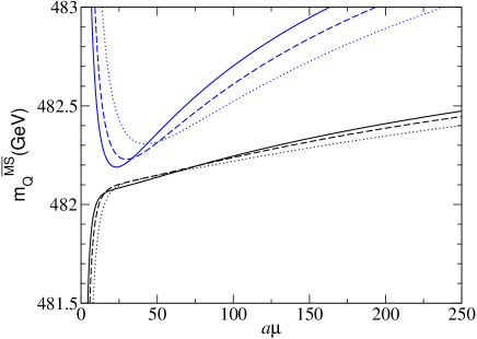
Figure 4: The RG scale dependence of $\overline{\rm MS}$ mass determined in the PCM. The dotted, dashed, and solid lines are at lattice spacings $a^{-1}=2.12,2.91,$ and $3.85$, respectively. The upper three lines are for the NLO and the lower three lines are for the NNLO results.

We first notice that the $\overline{\rm MS}$ masses at NLO have a RG scale dependence of $O(1\,{\rm GeV})$ over the range $1/a\leq\mu\leq m_{\rm Q}$, and the dependence on the lattice spacing about a few hundred MeVs. The NNLO results show improvement but still the scale dependence is about several hundred MeVs while the dependence on the lattice spacing is rather small, below 100 MeV, but still much larger than the uncertainty in the $\bar{\Lambda}^{\rm BR}$. Thus the uncertainties in the $\overline{\rm MS}$ masses from the PCM should be, at least, several hundred MeVs, much larger than in the BR method. Even if one evaluates the $\overline{\rm MS}$ mass at the optimal scale at which the differences between the NLO and NNLO results become minimal the obtained $\overline{\rm MS}$ masses will be larger by more than 100 MeV than those of the BR method.

Clearly, the strong dependence on the RG scale as well as on the lattice spacing in the PCM comes from the scale mixing, and this example shows that it can cause problems in systems with a large scale separation. The BR scheme solves this problem by isolating the heavy quark mass scale to the BR mass and the soft scale, in this case the lattice spacing, to the BR binding energy only, resulting in a greatly improved heavy quark mass determination. A good candidate to which the BR scheme can be applied is the top threshold production, where the cross section is computed from the Green’s function obtained by solving a Schroedinger equation involving a short-distance mass and a renormalon-subtracted heavy-quark potential, which again is plagued by the scale mixing between the top quark mass and the interquark distance  Hoang et al. (2000). Our Borel summation can help this problem by summing the renormalons in the top pole mass and the interquark potential independently, resulting in a Schroedinger equation involving the BR top-quark mass and interquark potential. Here again the hard scale, the top mass, is confined to the BR mass and the soft scale, the interquark distance, to the BR potential only, giving rise to a complete scale isolation. With the PCM, on the other hand, it may be necessary to resum the $\log(v)$ terms arising from the scale mixing  Hoang et al. (2001), where $v$ denotes the heavy quark velocity, but with the BR scheme this problem does not appear from the beginning.

To conclude, we have applied the Borel summation technique based on the bilocal expansion of the Borel transforms, which systematically takes into account the renormalon singularity as well as the usual perturbative expansions, to the heavy quark mass determination in lattice simulation. The exact nature of the renormalon cancellation in the BR scheme and the bilocal expansion allow us to define a calculable as well as physical pole mass and binding energy that are not short-distance quantities, and give rise to a most useful feature of the BR scheme, namely, the automatic isolation of the soft and hard scales in the system. We have observed that this scale isolation results in a more consistent determination of the heavy quark mass than based on the PCM, and this becomes more visible as the system comes to have a bigger hierarchy in scale. Although we have focused more on the practical advantages of the BR scheme, we wish to emphasize that its more important aspect is that it solves the conceptual difficulty with the long-distance quantities, and bring them to our avail.