S-wave and P-wave non-strange baryons in the  potential model of QCD.

Abstract

In this paper, we study the nucleon energy spectrum in the ground-state (with orbital momentum $L=0$) and the first excited state ($L=1$). The aim of this study is to find the mass and mixing angles of excited nucleons using a potential model describing QCD. This potential is of the “Coulombian+ linear” type and we take into account some relativistic effects, namely we use essentially a relativistic kinematic necessary for studying light flavors. By this model, we found the proton and $\Delta(1232)$ masses respectively equal to ($968MeV$, $1168MeV$), and the masses of the excited states are between $1564MeV$ and $1607MeV$.

1 Introduction

In the quark model, the baryons are represented as bound states of three quarks, confined by strong forces. Quantum Chromodynamics (QCD) aknowledged as the theory of strong interactions, is however not able to describe unambigously the strong-coupling regime, which requests alternative theories, like Flux-Tube model, Bag model, QCD string model, Lattice QCD, or phenomenological potential models. We will use in this work a phenomenological potential model describing explicitely the QCD characteristics, and taking into account some relativistic effects.

The potential model is essentially motivated by the experiment, and its wave functions are used to represent the states of strong interaction and to describe the hadrons. The most used is the harmonic oscillator potential which requires very simple calculations and qualitatively in agreement with the experimental data; on the other hand, the most usual potential models are using non relativistic kinematics, which is convenient for the heavy flavors systems, but cannot be suitable for the hadrons containing light flavors.

In this paper, we study the non-strange baryons spectrum in two different orbital momentum states within a quark model framework. We calculate the mass of baryons in the ground-state ($L=0$) with positive parity, and in the first excited state ($L=1$) with negative parity. The method used is variational calculation using Schrödinger equation. The baryon being a three-quarks system, we expose a three-body problem, and the method used to resolve it.

In section 2, we first introduce the Hamiltonian of our system. We use a potential of the “Coulombian+linear” form, which reproduces well the confinement and asymptotic freedom in QCD. For the kinetic part of our Hamiltonian, we have added a semi-relativistic correction.

In section 3, we develop the wave function of our system corresponding to ground-state using Jacobi variables. Then we diagonalize the Hamiltonian matrix and minimise it to extract the baryon mass value. To improve this value, we add the hyperfine correction which contains two terms. The first one (called the contact term) takes into account the spin-spin interaction, and it correlates the splitting of $\Delta-N$, $\Sigma-\Lambda$ in the ground state. The second one, called the tensor term, averages to zero for orbital momentum $L=0$.

In section 4, we study the case of P-wave baryons with negative parity. We use the same development as for the S-wave baryons to extract masses for the first excited state $L=1$. In this case, the tensor term is operative, and allows us to obtain mixing angles. Our results are then compared with the work of Isgur and Karl [1].

2 Potential model of QCD  

Several potential models were carried out until now for the determination of the baryon mass spectrum in non-perturbative QCD. In general, one uses the harmonic oscillator ([1], [2]) approach in the quark model . The result obtained is in agreement with the experimental data. This approach provides a good determination of ground state and excited states of the baryon energy spectrum. The Hamiltonian used is in the form:

$$H_{HO}=\sum_{i<j=1}^{3}(E_{i}+V_{HO}(r_{ij})+H_{hyp})$$ (1)

Where $E_{i}$ is the kinetic part, and the harmonic oscillator potential is in the following form :

$$V_{HO}(r_{ij})=\frac{1}{2}K\left|\overrightarrow{r_{i}}-\overrightarrow{r_{j}}\right|^{2}$$ (2)

$H_{hyp}$ represents the hyperfine correction.

A more appropriate potential is to be the so-called ”Coulombic+ linear” one: complicated non-perturbative effects are assumed to be largely absorbed into the constituent quark masses and into a Lorentz scalar linear confinement potential, the known short range behaviour of QCD is included in the one gluon exchange ”Coulombic” potential. In this approach the potential is defined as follows [3]:

$$V(r_{ij})=-(-\frac{\alpha_{s}}{r_{ij}}+\frac{3}{4}\sigma r_{ij}+\frac{3}{4}c)F_{i}.F_{j}$$ (3)

The $F_{i}.F_{j}$ factor represents the color term, with $\alpha_{ij}=$ $\left\langle F_{i}.F_{j}\right\rangle=-\frac{2}{3}$.

The constants ($\alpha_{s}$, $\sigma$, c) are the phenomenological parameters determined from an experimental fit.

In the present work, the calculation of the non-strange baryons spectrum is carried out, by using the parameters of reference [4]. The results obtained will be discussed in sections 3 and 4.

2.1 Variational Calculation

The kinetic energy of the relativistic Schrödinger equation describing a system with three quarks is in the form :

$$E_{i}=\sqrt{P_{i}^{2}+m_{i}^{2}}$$ (4)

But another term, essentially relativistic and more convenient for many-body problems than the kinetic part of the Hamiltonian given by equation (4), can be used:

$$(\frac{P_{i}^{2}}{2M_{i}}+\frac{M_{i}}{2}+\frac{m_{i}^{2}}{2M_{i}})$$

with the conditions:

$$\frac{\partial E}{\partial M_{i}}=0$$

as in reference [5], [7]. $M_{i}$ represents the quark dynamical masses. They are heavier than the quark constituent masses $m_{i}$.

The Hamiltonian of the system is thus written ([9], [10]) :

$$H=\sum_{i<j=1}^{3}\left[(\frac{P_{i}^{2}}{2M_{i}}+\frac{M_{i}}{2}+\frac{m_{i}^{2}}{2M_{i}})+V(r_{ij})\right]$$ (5)

The calculation of the total energy of the system is carried out by the variational method. This energy will be minimized w.r.t the variational parameters of the test wave function and ($M_{i}$).
The potential $V(r_{ij})$ is treated overall here like a non-perturbative term. In reference [8], $V(r_{ij})$ is written in the form of harmonic oscillator potential ($Kr_{ij}^{2}/2$) plus an unknown U-term (treated like a perturbation) added to shift the energies of some states (using the oscillator harmonic wave function).

In our work, we concentrate on the determination of the ground-state nucleon mass, by minimizing the total energy. This method allows us to fix the auxiliary dynamical masses ($M_{i}$) and the wave function parameters. We use the same method to determine the excited-state nucleon mass. The wave function parameter and $M_{i}$ found for $L=0$ are different from the ones found for $L=1$.

2.2 The three-body problem

The baryon being a three-body system, so the problem is in the calculation of the energy eigenvalue, which contains an integral of nine variables. Before choosing the form of the test wave function, one defines the coordinates of Jacobi $(\overrightarrow{\rho},\overrightarrow{\lambda})$, which make it possible to pass from a three-body system to an equivalent two-body system. These two relative coordinates represent respectively the distance between the first two quarks ($q_{1,}q_{2}$), and the distance between the third quark $q_{3}$ and the center of mass of the system $q_{1}q_{2}$. The Jacobi coordinates are defined as [2] :

$$\ \overrightarrow{\rho} = \frac{1}{\sqrt{2}}(\overrightarrow{r_{1}}-\overrightarrow{r_{2}})$$ (6)

$$\overrightarrow{\lambda} = \frac{1}{\sqrt{6}}(\overrightarrow{r_{1}}+\overrightarrow{r_{2}}-2\overrightarrow{r_{3}})$$

Using these coordinates, we obtain the relative Hamiltonian $H_{R}$ written in the following form:

$$H_{R}=\frac{P_{\rho}^{2}}{2\mu_{\rho}}+\frac{P_{\lambda}^{2}}{2\mu_{\lambda}}+M_{u}+\frac{m_{u}^{2}}{M_{u}}+\frac{M_{d}}{2}+\frac{m_{d}^{2}}{2M_{d}}+V(\overrightarrow{\rho},\overrightarrow{\lambda})$$ (7)

With :

$\mu_{\rho}=M_{u}$          ($u$ and $d$ represent the quark flavors)

$\mu_{\lambda}=\frac{3M_{u}M_{d}}{2M_{u}+M_{d}}$

The potential $V(\overrightarrow{\rho},\overrightarrow{\lambda})$ is written in the form

$$V(\overrightarrow{\rho},\overrightarrow{\lambda}) = -\frac{2\alpha_{s}}{3}\left(\frac{1}{\sqrt{2}\rho}+\frac{1}{\frac{1}{\sqrt{2}}\left|\sqrt{3}\overrightarrow{\lambda}+\overrightarrow{\rho}\right|}+\frac{1}{\frac{1}{\sqrt{2}}\left|\sqrt{3}\overrightarrow{\lambda}-\overrightarrow{\rho}\right|}\right)$$

$$+\frac{\sigma}{2}\left(\sqrt{2}\rho+\frac{1}{\sqrt{2}}\left|\sqrt{3}\overrightarrow{\lambda}+\overrightarrow{\rho}\right|+\frac{1}{\sqrt{2}}\left|\sqrt{3}\overrightarrow{\lambda}-\overrightarrow{\rho}\right|\right)-2c$$

3 Application of the model to the S-wave baryon

In this part, one concentrates on the determination of the ground-states masses of non-strange baryons with orbital momentum L=0. The parameter of the wave function and masses ($M_{u}$, $M_{d}$) are determined using the variational treatment.

3.1 Determination of the proton wave function

The total wave function $\left|qqq\right\rangle$ of the system is in general constructed from the sum of $C_{A}\sum\chi\Psi\Phi$, where $\left(C_{A},\chi,\Psi,\Phi\right)$ represent respectively the color, spin, spatial and flavor wave functions, with $C_{A}$ totally antisymmetric.

$$\left|qqq\right\rangle\ =\left|Color\right\rangle_{A}\ \times\left|Spatial,Spin,Flavor\right\rangle_{S}\$$

The indices $A$ and $S$ mean the antisymmetry and symmetry under the exchange of any pair of quarks of equal masses.

$$\left|N^{2}S_{S}\frac{1}{2}^{+}\right\rangle = C_{A}\Psi^{S}_{00}\frac{1}{\sqrt{2}}(\Phi^{\rho}_{N}\chi^{\rho}_{\frac{1}{2}}+\Phi^{\lambda}_{N}\chi^{\lambda}_{\frac{1}{2}})$$ (9)

$$\left|\Delta^{4}S_{S}\frac{3}{2}^{+}\right\rangle = C_{A}\Phi^{S}_{\Delta}\Psi^{S}_{00}\chi^{S}_{\frac{3}{2}}$$

One restricts oneself here to the spatial wave function for the calculation carried out with the Hamiltonian $H_{R}$. To calculate the hyperfine correction, one will take the total wave function defined in section $4$. These corrections will give us the mass splitting between nucleon and $\Delta(1232)$. The spatial wave function $\Psi_{00}$ selected to describe our system in the fundamental state $\left(\Psi_{LM}\longrightarrow L=0\text{, }M=0\right)$, is a Gaussian that one develops on the possible states of the angular momenta of the systems $q_{1}q_{2}$ and $q_{3}$. These states are indexed by $\mid l_{\rho}$, $l_{\lambda}\rangle$ with $\overrightarrow{L}=\overrightarrow{l_{\rho}}+\overrightarrow{l_{\lambda}}$ . The spatial wave function used in our calculation is in the following form:

$$\Psi_{LM}(\overrightarrow{\rho},\overrightarrow{\lambda}) = \underset{l_{\rho},l_{\lambda}}{\sum}\underset{m_{\rho},m_{\lambda}}{\sum}C_{l_{\rho}l_{\lambda}}.N_{l_{\rho}l_{\lambda}}\left\langle l_{\rho}m_{\rho}l_{\lambda}m_{\lambda}\mid LM\right\rangle\times\rho^{l_{\rho}}\lambda^{l_{\lambda}}\$$

$$\times Exp[-\frac{1}{2}(\alpha_{\rho}^{2}\rho^{2}+\alpha_{\lambda}^{2}\lambda^{2})]Y_{l_{\rho}}^{m_{\rho}}(\Omega_{\rho})Y_{l_{\lambda}}^{m_{\lambda}}(\Omega_{\lambda})$$

where $C_{l_{\rho}l_{\lambda}}$ are coefficients determined by diagonalisation of the $H_{R}$ matrix. The minimization of the system energy allows the determination of the variational parameters of the spatial wave function $(\alpha_{\rho},\alpha_{\lambda})$ and the dynamical masses $(M_{u},M_{d})$. The average value of the energy over the function $\Psi_{00}$ is given by the following relation:

$$E(\alpha_{\rho},\alpha_{\lambda},M_{i})=\frac{\left\langle\Psi_{00}\right|H_{R}\left|\Psi_{00}\right\rangle}{\left\langle\Psi_{00}\mid\Psi_{00}\right\rangle}$$ (11)

The only Clebsch-Gordan coefficients different from zero are those which couple the orbital momentum associated to the Jacobian coordinates ($\overrightarrow{\rho},\overrightarrow{\lambda}$) with the total orbital momentum $L=0$, and we have:

$$|l_{\rho}-l_{\lambda}|\leq L=0\leq l_{\rho}+l_{\lambda}$$ (12)

The expression (12) yields the constraint ($l_{\rho}=l_{\lambda}$). So the states of this subsystem ($\overrightarrow{\rho},\overrightarrow{\lambda}$) which contribute to the spatial wave function have all the same orbital momentum, starting with $l_{\rho}=l_{\lambda}=0$. From parity we have $P=(-)^{L}=(-)^{l_{\rho}+l_{\lambda}}=+1$, so ($l_{\rho}+l_{\lambda}$) is even. We do our treatment up to order $2$, i.e. $l_{\rho}=l_{\lambda}=2$, since for higher orders the analytical calculation becomes very complicated, moreover the contribution of the orbital momentum terms $l>2$ is less important [11]. The total wave function must obey the Pauli Exclusion Principle. In the baryon we have two identical quarks, so the spatial wave function must be symmetrical in the exchange of these two quarks $r_{1}\longleftrightarrow r_{2}$, this implies that in the relative system, the function should be even in $\rho$ ($\overrightarrow{\rho}=\frac{1}{\sqrt{2}}(\overrightarrow{r_{1}}-\overrightarrow{r_{2}})$). So in expression (3.1), $l_{\rho}$ must be even.

Finally, by eliminating the contribution of the odd states in $l_{\rho}$, only two terms contribute to the construction of the spatial wave function, which is a superposition of $\left|l_{\rho}=0,l_{\lambda}=0\right\rangle$ and $\left|l_{\rho}=2,l_{\lambda}=2\right\rangle$. So the calculation of energy reduces to the calculation of the matrix elements of $H_{R}$ on the states $\left|l_{\rho},l_{\lambda}\right\rangle=\left|00\right\rangle$ and $\left|22\right\rangle$.

If one notes the spatial wave function in the representation of Dirac, one will have:

$$\left|\Psi_{00}\right\rangle=c_{1}\left|00\right\rangle+c_{2}\left|22\right\rangle$$ (13)

Equation (13) shows that the physical state is a mixing of the relative orbital momentum states ($l_{\rho}$,$l_{\lambda}=0,0$) and ($l_{\rho}$,$l_{\lambda}=2,2$), with mixing coefficients (c1, c2). To calculate the energy of the physical state $\left|\Psi_{00}\right\rangle$, one starts by evaluating the matrix elements of $H_{R}$ on the base {$\left|00\right\rangle$, $\left|22\right\rangle$}. The $2\times 2$ matrix is not diagonal. If one notes $T$ the kinetic energy and $V$ the potential energy, the $H_{R}$ matrix is written:

$$H_{R}=\left(\begin{array}[]{cc}H_{R}^{(00,00)}&H_{R}^{(00,22)}\\ H_{R}^{(22,00)}&H_{R}^{(22,22)}\end{array}\right)=\left(\begin{array}[]{cc}\left\langle 00\right|(T+V)\left|00\right\rangle&\left\langle 00\right|V\left|22\right\rangle\\ \left\langle 22\right|V\left|00\right\rangle&\left\langle 22\right|(T+V)\left|22\right\rangle\end{array}\right)$$ (14)

It should be noted that by analogy with the work of Capstick [8], one has $\alpha_{\rho}$ $\simeq\alpha_{\lambda}$, because in the case of the harmonic oscillator $\alpha_{\rho}$ and $\alpha_{\lambda}$ are proportional to the masses $m_{u}$ and $m_{d}$ in the case of baryons with the same quark masses. So one replaces in the function $\left|\Psi_{00}\right\rangle$, $\alpha_{\rho}$ $=\alpha_{\lambda}=\alpha$. The calculation of the elements $T_{l_{\rho}l_{\lambda},l_{\rho}^{\prime}l_{\lambda}^{\prime}}$ is treated in detail in appendix (6.2). The non-zero elements are the two diagonal elements $T_{00,00}$ and $T_{22,22}$. These elements are thus given according to ($\alpha$, $M_{u}$,$M_{d}$).

The calculation of the matrix elements of the potential energy requires to evaluate an integral of dimension six on the potential $V(\overrightarrow{\rho},\overrightarrow{\lambda})$ which contains terms coupled in ($\rho,\lambda$) and the angle $\theta$ between the two vectors $(\overrightarrow{\rho},\overrightarrow{\lambda})$, see fig(1).

Figure 1: Relative coordinates $\vec{\rho}$ and $\vec{\lambda}$

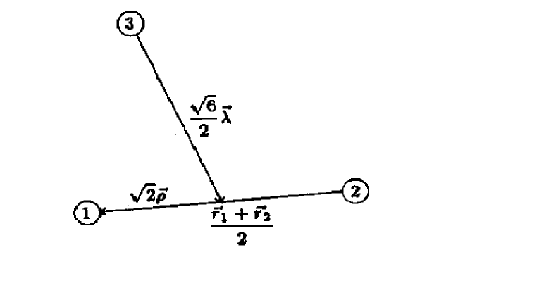
With :

$$r_{12} = \sqrt{2}\rho$$ (15)

$$r_{13} = \frac{1}{\sqrt{2}}\sqrt{\rho^{2}+\sqrt{3}\overrightarrow{\rho}.\overrightarrow{\lambda}+3\lambda^{2}}$$

$$r_{23} = \frac{1}{\sqrt{2}}\sqrt{\rho^{2}-\sqrt{3}\overrightarrow{\rho}.\overrightarrow{\lambda}+3\lambda^{2}}$$

and using the form of “Coulombian+ Linear” potential in equation (2.2)

one calculates now the matrix elements:

$$\left\langle LM\right|V(\overrightarrow{\rho},\overrightarrow{\lambda})\left|L^{\prime}M^{\prime}\right\rangle = \underset{m_{\rho},m_{\lambda}}{\underset{l_{\rho},l_{\lambda}}{\sum}}\underset{m_{\rho}^{\prime},m_{\lambda}^{\prime}}{\underset{l_{\rho}^{\prime},l_{\lambda}^{\prime}}{\sum}}\left\langle l_{\rho}m_{\rho}l_{\lambda}m_{\lambda}|LM\right\rangle^{\ast}\left\langle l_{\rho}^{\prime}m_{\rho}^{\prime}l_{\lambda}^{\prime}m_{\lambda}^{\prime}|L^{\prime}M^{\prime}\right\rangle$$

$$\times\int d\overrightarrow{\rho}d\overrightarrow{\lambda}\rho^{l_{\rho}+l_{\rho}^{\prime}}\lambda^{l_{\lambda}+l_{\lambda}^{\prime}}Exp\left[-\alpha^{2}(\rho^{2}+\lambda^{2})\right]V(\overrightarrow{\rho},\overrightarrow{\lambda})$$

$$\times Y_{l_{\rho}}^{m_{\rho}\ast}\left(\Omega_{\rho}\right)Y_{l_{\lambda}}^{m_{\lambda}\ast}\left(\Omega_{\lambda}\right)\ Y_{l_{\rho}^{\prime}}^{m_{\rho}^{\prime}}\left(\Omega_{\rho}\right)Y_{l_{\lambda}^{\prime}}^{m_{\lambda}^{\prime}}\left(\Omega_{\lambda}\right)$$

To evaluate this integral in the coordinate system ($\overrightarrow{\rho},\overrightarrow{\lambda}$) , one

uses the hyperspherical coordinates ($\xi,\theta$) defined as follows :

$$\rho = \xi\sin(\theta)$$ (17)

$$\lambda = \xi\cos(\theta)$$

This implies that : $\ \xi^{2}=\rho^{2}+\lambda^{2}$ and $\theta=arctg(\frac{\rho}{\lambda})$, $0\leq\theta\leq\frac{\pi}{2}$

The integral (3.1) can be simplified in the following form:

$$V_{l_{\rho}l_{\lambda},l_{\rho}^{\prime}l_{\lambda}^{\prime}}=\int\limits_{0}^{\infty}d\xi\xi^{5}\left(\frac{\xi}{2}\sigma A_{l_{\rho}l_{\lambda},l_{\rho}^{\prime}l_{\lambda}^{\prime}}+\frac{2}{3\xi}\alpha_{s}B_{l_{\rho}l_{\lambda},l_{\rho}^{\prime}l_{\lambda}^{\prime}}-2c\right)R_{l_{\rho}l_{\lambda}}(\xi)R_{l_{\rho}^{\prime}l_{\lambda}^{\prime}}(\xi)$$ (18)

With :

$$\ R_{l_{\rho}l_{\lambda}}(\xi)=K_{l_{\rho}l_{\lambda}}\ \xi^{l_{\rho}+l_{\lambda}}Exp\left[-\frac{1}{2}\alpha^{2}\xi^{2}\right]$$

$K_{l_{\rho}l_{\lambda}}$is a normalization factor. The problem now amounts to the determination of elements $A_{l_{\rho}l_{\lambda},l_{\rho}^{\prime}l_{\lambda}^{\prime}}$ and $B_{l_{\rho}l_{\lambda},l_{\rho}^{\prime}l_{\lambda}^{\prime}}$. These elements represent the angular part in the integral (3.1). The method carried out by calculation of $A_{l_{\rho}l_{\lambda},l_{\rho}^{\prime}l_{\lambda}^{\prime}}$ and $B_{l_{\rho}l_{\lambda},l_{\rho}^{\prime}l_{\lambda}^{\prime}}$ is developed in detail in appendix (6.3).

3.2 Mass of the proton and mixing coefficients

The analytic form of the Hamiltonian matrix elements of equation (14) is:

$$H^{(00,00)}_{R} = \frac{1}{2}\{-1.74320+\frac{m_{d}^{2}}{M_{d}}+M_{d}+\frac{2m_{u}^{2}}{M_{u}}+2M_{u}$$ (19)

$$+\frac{0.737249}{\alpha}-2.74449\alpha+\alpha^{2}(\frac{1}{M_{d}}+\frac{2}{M_{u}})\}$$

$$H^{(00,22)}_{R} = (0.04396-0.08154)\frac{1}{\alpha}$$ (20)

$$H^{(22,00)}_{R} = H^{(00,22)}_{R}$$ (21)

$$H^{(22,22)}_{R} = -0.87160+\frac{0.5m_{d}^{2}}{M_{d}}+0.5M_{d}+\frac{m_{u}^{2}}{M_{u}}+M_{u}$$

$$+\frac{0.114109}{\alpha}-0.181177\alpha+(\frac{1.16667}{M_{d}}+\frac{2.33333\alpha^{2}}{M_{u}})\alpha^{2}$$

After diagonalisation and minimization of the Hamiltonian matrix, we find the following result (using an algorithm of Mathematica $5.0$ program) :

$E_{min}^{1}=1068MeV$ $\longleftarrow$ ($\alpha=200MeV$, $M_{u}=M_{d}=480MeV$)

$E_{min}^{2}=1412MeV$ $\longleftarrow$ ($\alpha=337MeV$, $M_{u}=M_{d}=580MeV$)

The physical state energy is the lowest value of these two eigenvalues ($E_{min}^{1}$,$E_{min}^{2}$). Table (1) gives the parameters of the potential model considered in this work, which were used in [4]. The results of the computation of the nucleon and $\Delta(1232)$ mass are summarized in table (2) as well as the values of the variational parameters ($\alpha$, $M_{u}$, $M_{d}$). These parameters will be used in the calculation of the corrections of the spin-spin type in the semi-relativistic model (cf. section 3.3).

It should be noted here that the mass of both nucleon and $\Delta(1232)$ appearing in table (2) is the energy of the physical state, which is a mixing of the states $\left|00\right\rangle$ and $\left|22\right\rangle$, where the coefficients of the mixing obtained after diagonalisation, are given by:

$$\left|N,\Delta\right\rangle=0.9761\left|00\right\rangle-0.2673\left|22\right\rangle\longrightarrow E_{N,\Delta}=1068MeV$$ (23)

3.3 Hyperfine interaction and calculation of the baryons masses

The potential of the hyperfine interaction is composed of two terms ([12],[13]) :

$$V_{hyp}=V_{c}+V_{t}$$ (24)

Where the first term (called contact term of Fermi), represents the spin-spin interaction between the quarks in the baryon. It is operative only in the fundamental state, where the orbital momentum is equal to zero.

$$V_{c}=-\sum_{i<j=1}^{N}\alpha_{ij}\frac{8\pi\alpha_{h}}{3M_{i}M_{j}}\frac{\sigma_{h}^{3}}{\sqrt{\pi^{3}}}\exp(-\sigma_{h}^{2}r_{ij}^{2})S_{i}.S_{j}$$ (25)

$(\alpha_{h},\sigma_{h})$ are parameters fitted in reference [4], (see table(1)). The second term (called tensor term) represents the static interaction of two intrinsic magnetic dipoles. It is operative only if the orbital momentum is larger than zero. It is written in the form:

$$V_{t}=\sum_{i<j=1}^{N}\alpha_{ij}\frac{\alpha_{s}}{M_{i}M_{j}}\frac{1}{r_{ij}^{3}}\left(3(S_{i}.r)(S_{i}.r)-S_{i}.S_{j}\right)$$ (26)

This term enables us to have the mixing coefficients of non-strange baryons ($S=0$) in the $P$ wave ($L=1$). The first term $V_{c}$ enables us to separate between baryons of the same $J^{P}$ but of different spin. From equations {(9), (25)}, we obtain the mass of the nucleon and $\Delta(1232)$ (mass splitting $\Delta-N$). Table (2) shows the results obtained for the baryons masses, with and without hyperfine correction.

$\alpha_{h}$	$\sigma_{h}$	$\alpha_{s}$	$\sigma$	$\frac{3}{4}c(MeV)$	$m_{u}(MeV)$	$m_{d}(MeV)$
0.840	0.700	0.857	0.154	-436	375	375

Table 1: Parameters of the quark potential model [4]

	$\alpha$	$M_{u}$	$M_{d}$	$M_{0}$	$M_{cor}$	$Exp$
$N(\frac{1}{2}^{+})$	200	480	480	1068	968	938
$\Delta(\frac{3}{2}^{+})$	200	480	480	1068	1168	1232

Table 2: The ground-state energy of baryons (in MeV). $M_{0}$ is the baryon mass without hyperfine correction and $M_{cor}$ represents the baryon mass with spin-spin ($V_{c}$) correction.

4 Application of the model to the P-wave baryon

One carries out now the calculation of the first excited state energy of the baryon with $L=1$ and negative parity, using the same method as for the S-wave. In this case one will build the total wave function, which has to be antisymmetric.

4.1 Determination of the wave function for $L=1$

In the construction of the spatial wave function, the only possible states for $(l_{\rho},l_{\lambda})$ which allow to have an orbital momentum L=1 and negative parity are $(l_{\rho}=1,l_{\lambda}=0)$ and $(l_{\rho}=0,l_{\lambda}=1)$ which are noted respectively ($\Psi_{1M}^{\rho}$, $\Psi_{1M}^{\lambda}$). Note from equation (6) that $\Psi_{1M}^{\lambda}$ is even under the exchange of the first two quarks, while the analogous wave function $\Psi_{1M}^{\rho}$ is odd, since $\rho$ and $\lambda$ respectively indicate mixed antisymmetry and mixed symmetry under this transposition. These states form a representation of dimension two of the permutation group $S_{3}$, which allows to exchange each pair of quarks in the baryon.

These two functions have the following form:

$$\Psi^{\rho}_{1M}(\overrightarrow{\rho},\overrightarrow{\lambda}) = C_{10}\underset{m_{\rho},m_{\lambda}}{\sum}N_{10}\left\langle 1m_{\rho}0m_{\lambda}\mid 1M\right\rangle$$ (27)

$$\times\mathbf{\rho}Exp[-\frac{1}{2}\alpha^{2}(\rho^{2}+\lambda^{2})]Y_{1}^{m_{\rho}}(\Omega_{\rho})Y_{0}^{m_{\lambda}}(\Omega_{\lambda})$$

$$\Psi^{\lambda}_{1M}(\overrightarrow{\rho},\overrightarrow{\lambda}) = C_{01}\underset{m_{\rho},m_{\lambda}}{\sum}N_{01}\left\langle 0m_{\rho}1m_{\lambda}\mid 1M\right\rangle$$

$$\times\mathbf{\lambda}Exp[-\frac{1}{2}\alpha^{2}(\rho^{2}+\lambda^{2})]Y_{0}^{m_{\rho}}(\Omega_{\rho})Y_{1}^{m_{\lambda}}(\Omega_{\lambda})$$

One will have also to consider the coupling of the spins $S$ with the orbital momentum $L$ to build the total angular momentum $\overrightarrow{J}=\overrightarrow{L}+\overrightarrow{S}$. In short, here is the construction of $J$:

The spin of the quark system : $S=\frac{1}{2},\frac{3}{2}$ , is constructed as the triple product $\left(\frac{1}{2}\otimes\frac{1}{2}\otimes\frac{1}{2}\right).$

One has $L=1$, one thus distinguishes two constructions of $J$ for the doublet and the quadruplet of spin :

$1)$ $S=\frac{1}{2}$, $L=1\longrightarrow$ ${}^{2}P_{\frac{1}{2}}$, ${}^{2}P_{\frac{3}{2}}$,     $J^{P}=\frac{1}{2}^{-},\frac{3}{2}^{-}$

$2)$ $S=\frac{3}{2}$, $L=1\longrightarrow$ ${}^{4}P_{\frac{1}{2}}$, ${}^{4}P_{\frac{3}{2}}$, ${}^{4}P_{\frac{5}{2}}$,    $J^{P}=\frac{1}{2}^{-},\frac{3}{2}^{-},\frac{5}{2}^{-}$

The nucleon states of total angular momentum $J=\frac{1}{2},\frac{3}{2}$ are a mixing of the doublet and quadruplet of spin, for example:

$$\left|J^{P}=(\frac{1}{2})^{-}\right\rangle = \alpha_{1}\left|{}^{4}P_{\frac{1}{2}}\right\rangle+\beta_{1}\left|{}^{2}P_{\frac{1}{2}}\right\rangle$$ (28)

$$\left|J^{P}=(\frac{3}{2})^{-}\right\rangle = \alpha_{2}\left|{}^{4}P_{\frac{3}{2}}\right\rangle+\beta_{2}\left|{}^{2}P_{\frac{3}{2}}\right\rangle$$

Thus, the wave function will be built as :

$$\left|{}^{2}P_{\frac{1}{2}}\right\rangle \sim \sum\Psi_{1M}\chi_{\frac{1}{2}}\Phi$$ (29)

$$\left|{}^{4}P_{\frac{1}{2}}\right\rangle \sim \sum\Psi_{1M}\chi_{\frac{3}{2}}\Phi$$

The construction of the spin-flavor wave function is carried out in analogy with the notation of Karl and Isgur and collaborators ([1], [8]). The flavor-mixed antisymmetry and symmetry combinations of “$uud$” are:

$$\Phi_{p}^{\rho} = \frac{1}{\sqrt{2}}(udu-duu)$$ (30)

$$\Phi_{p}^{\lambda} = -\frac{1}{\sqrt{6}}(duu+udu-2uud)$$

In the same way, the spin states are:

$$\chi_{\frac{1}{2}}^{\rho} = \frac{1}{\sqrt{2}}(\left|\uparrow\downarrow\uparrow\right\rangle-\left|\downarrow\uparrow\uparrow\right\rangle)$$ (31)

$$\chi_{\frac{1}{2}}^{\lambda} = -\frac{1}{\sqrt{6}}(\left|\downarrow\uparrow\uparrow\right\rangle+\left|\uparrow\downarrow\uparrow\right\rangle-2\left|\uparrow\uparrow\downarrow\right\rangle)$$

One must add the spin wave function for the quadruplet which is completely symmetric:

$$\chi_{\frac{3}{2}}^{S}=\left|\uparrow\uparrow\uparrow\right\rangle$$ (32)

Thus, the total wave function will be built according to the following combinations:

$$\left|N^{2}P_{M}(\frac{1}{2}^{-},\frac{3}{2}^{-})\right\rangle = C_{A}\frac{1}{2}[\Phi^{\rho}_{N}(\Psi^{\rho}_{1M}\chi^{\lambda}_{\frac{1}{2}}+\Psi^{\lambda}_{1M}\chi^{\rho}_{\frac{1}{2}})+\Phi^{\lambda}_{N}(\Psi^{\rho}_{1M}\chi^{\rho}_{\frac{1}{2}}-\Psi^{\lambda}_{1M}\chi^{\lambda}_{\frac{1}{2}})]$$

$$\left|N^{4}P_{M}(\frac{1}{2}^{-},\frac{3}{2}^{-})\right\rangle = C_{A}\chi^{S}_{\frac{3}{2}}\frac{1}{\sqrt{2}}(\Phi^{\rho}_{N}\Psi^{\rho}_{1M}+\Phi^{\lambda}_{N}\Psi^{\lambda}_{1M})$$ (33)

$$\left|\Delta^{2}P_{M}(\frac{1}{2}^{-},\frac{3}{2}^{-})\right\rangle = C_{A}\Phi^{S}_{\Delta}\frac{1}{\sqrt{2}}(\Psi^{\rho}_{1M}\chi^{\rho}_{\frac{1}{2}}+\Psi^{\lambda}_{1M}\chi^{\lambda}_{\frac{1}{2}})$$

From equation (33), one sees that we have two groups of states: $N^{\ast}$ and $\Delta^{\ast}$. Each group has its own flavor wave function.

4.2 Excited nucleon mass

For the P-wave excited-state nucleon, the Hamiltonian matrix is written as follows:

$$H_{R}=\left(\begin{array}[]{cc}\left\langle 01\right|H_{R}\left|01\right\rangle&\left\langle 01\right|H_{R}\left|10\right\rangle\\ \left\langle 10\right|H_{R}\left|01\right\rangle&\left\langle 10\right|H_{R}\left|10\right\rangle\end{array}\right)$$ (34)

By the same method used in calculation of the baryons masses in the ground-state $L=0$, one finds the elements of the $H_{R}$ matrix for $L=1$:

$$\left\langle 01\right|H_{R}\left|01\right\rangle = \frac{1}{2}(-1.7432+\frac{0.7372}{\alpha}-2.7445\alpha+\frac{m_{d}^{2}}{M_{d}}+M_{d}$$

$$+\alpha^{2}(\frac{1}{M_{d}}+\frac{2}{M_{u}})+\frac{2m_{u}^{2}}{M_{u}})$$

$$\left\langle 01\right|H_{R}\left|10\right\rangle = \left\langle 10\right|H_{R}\left|01\right\rangle$$

$$= (0.0439-0.0815\alpha^{2})\frac{1}{\alpha}$$

$$\left\langle 10\right|H_{R}\left|10\right\rangle = -0.8716+\frac{0.1141}{\alpha}-\frac{0.1812}{\alpha}+\frac{1.1667\alpha^{2}}{M_{d}}+\frac{m_{d}^{2}}{2M_{d}}+\frac{M_{d}}{2}$$ (35)

$$+\frac{2.3333\alpha^{2}}{M_{u}}+\frac{m_{u}^{2}}{M_{u}}+M_{u}$$

After diagonalisation of this matrix, one obtains two eigenvalues of the Hamiltonian $H_{R}$ :

$$H_{R}^{1} = \frac{1}{2}[-1.7432+\frac{m_{d}^{2}}{M_{d}}+M_{d}+\frac{2m_{u}^{2}}{M_{u}}+2M_{u}+\frac{0.2027}{\alpha}-1.0745\alpha$$

$$+(\frac{1.3333}{M_{d}}+\frac{2.6666}{M_{u}})\alpha^{2}-\{-0.2863+\frac{0.0310}{\alpha^{2}}-(\frac{0.0193}{M_{d}}+\frac{0.0193}{M_{u}})\alpha$$

$$+0.7850\alpha^{2}-(\frac{0.1433}{M_{d}}+\frac{0.1433}{M_{u}})\alpha^{3}+(\frac{0.1111}{M_{d}^{2}}+\frac{0.1111}{M_{u}^{2}}+\frac{0.2222}{M_{u}M_{d}})\alpha^{4}\}^{\frac{1}{2}}]$$

$$H_{R}^{2} = \frac{1}{2}[-1.7432+\frac{m_{d}^{2}}{M_{d}}+M_{d}+\frac{2m_{u}^{2}}{M_{u}}+2M_{u}+\frac{0.2027}{\alpha}-1.0745\alpha$$

$$+(\frac{1.3333}{M_{d}}+\frac{2.6666}{M_{u}})\alpha^{2}+\{-0.2863+\frac{0.0310}{\alpha^{2}}-(\frac{0.0193}{M_{d}}+\frac{0.0193}{M_{u}})\alpha$$

$$+0.7850\alpha^{2}-(\frac{0.1433}{M_{d}}+\frac{0.1433}{M_{u}})\alpha^{3}+(\frac{0.1111}{M_{d}^{2}}+\frac{0.1111}{M_{u}^{2}}+\frac{0.2222}{M_{u}M_{d}})\alpha^{4}\}^{\frac{1}{2}}]$$

The minimization of these two eigenvalues yields the following result :

$$H_{R}^{1}\to 1590\ MeV$$

$$H_{R}^{2}\to 1755\ MeV$$ (37)

The minimal value ($1594$ $MeV$) corresponds to the nucleon mass in the first excited state $L=1$ for the values ($\alpha=192MeV,M_{u}=M_{d}=1485MeV$). In order to separate between the nucleon states of different total angular momentum, one will apply the hyperfine potential defined in equation (24) which is composed of two parts, the contact term and the tensor term.

4.3 Hyperfine correction

The orbital excitation $L=1$ of the baryon is carried by only one pair of quarks, while the two other pairs have zero orbital momentum. This decomposition of orbital momentum enables us to note that the tensor part of the hyperfine interaction is operational only in the quark-pair with L=1. On the other hand, the two other pairs with orbital momentum equal to zero are controlled by the contact term of the hyperfine interaction. One will calculate first the contact part, then the tensor part.

4.3.1 The elements of the contact matrix

The following calculation was carried out for only one pair of quarks, then the result was multiplied by three. Furthermore the result does not depend on the total angular momentum. Recall that the total spin for our system takes the value ($S=\frac{1}{2}$, $S=\frac{3}{2}$) and thus we are left to calculate the elements of the following matrix :

$$\left(\begin{array}[]{cc}\left\langle N^{4}P_{M}(J)\right|V_{c}\left|N^{4}P_{M}(J)\right\rangle&\left\langle N^{4}P_{M}(J)\right|V_{c}\left|N^{2}P_{M}(J)\right\rangle\\ &\\ \left\langle N^{2}P_{M}(J)\right|V_{c}\left|N^{4}P_{M}(J)\right\rangle&\left\langle N^{2}P_{M}(J)\right|V_{c}\left|N^{2}P_{M}(J)\right\rangle\\ &\end{array}\right)$$ (38)

Using equation (33) one obtains:

$$\left\langle N^{4}P_{M}(J)\right|V_{c}\left|N^{4}P_{M}(J)\right\rangle = 3\left\langle N^{4}P_{M}(J)\right|V^{12}_{c}\left|N^{4}P_{M}(J)\right\rangle$$

$$= \frac{3}{2}\{\left\langle\chi^{s}_{\frac{3}{2}}\Psi^{\lambda}_{1M}\right|V^{12}_{c}\left|\chi^{s}_{\frac{3}{2}}\Psi^{\lambda}_{1M}\right\rangle$$

$$\ \ \ +\left\langle\chi^{s}_{\frac{3}{2}}\Psi^{\rho}_{1M}\right|V^{12}_{c}\left|\chi^{s}_{\frac{3}{2}}\Psi^{\rho}_{1M}\right\rangle\}$$

$$= \frac{3}{2}\frac{8\pi\alpha_{h}}{3M^{2}}\frac{2}{3}\frac{\sigma_{h}^{3}}{\sqrt{\pi^{3}}}\left\langle\chi^{s}_{\frac{3}{2}}\right|S_{1}.S_{2}\left|\chi^{s}_{\frac{3}{2}}\right\rangle$$

$$\times\{\left\langle\Psi^{\lambda}_{1M}\right|Exp(-\sigma_{h}^{2}r_{12}^{2})\left|\Psi^{\lambda}_{1M}\right\rangle$$

$$\ \ \ +\left\langle\Psi^{\rho}_{1M}\right|Exp(-\sigma_{h}^{2}r_{12}^{2})\left|\Psi^{\rho}_{1M}\right\rangle\}$$

$$\left\langle N^{2}P_{M}(J)\right|V_{c}\left|N^{2}P_{M}(J)\right\rangle = 3\left\langle N^{2}P_{M}(J)\right|V^{12}_{c}\left|N^{2}P_{M}(J)\right\rangle$$ (40)

$$= \frac{3}{2}\frac{8\pi\alpha_{h}}{3M^{2}}\frac{2}{3}\frac{\sigma_{h}^{3}}{\sqrt{\pi^{3}}}$$

$$\left(\left\langle\chi^{\rho}_{\frac{1}{2}}\right|S_{1}.S_{2}\left|\chi^{\rho}_{\frac{1}{2}}\right\rangle+\left\langle\chi^{\lambda}_{\frac{1}{2}}\right|S_{1}.S_{2}\left|\chi^{\lambda}_{\frac{1}{2}}\right\rangle\right)$$

$$\times(\left\langle\Psi^{\lambda}_{1M}\right|Exp(-\sigma_{h}^{2}r_{12}^{2})\left|\Psi^{\lambda}_{1M}\right\rangle$$

$$\ \ \ +\left\langle\Psi^{\rho}_{1M}\right|Exp(-\sigma_{h}^{2}r_{12}^{2})\left|\Psi^{\rho}_{1M}\right\rangle)$$

After integration of the spatial part, and using the Jacobi variable change $(\mathbf{r_{12}=\sqrt{2}\rho})$ one obtains the following result :

$$\left\langle\Psi^{\lambda}_{1M}\right|Exp(-\sigma_{h}^{2}r_{12}^{2})\left|\Psi^{\lambda}_{1M}\right\rangle = \left\langle\Psi^{\lambda}_{1M}\right|Exp(-2\sigma_{h}^{2}\rho^{2})\left|\Psi^{\lambda}_{1M}\right\rangle$$ (41)

$$= \frac{\alpha^{3}}{(\alpha^{2}+2\sigma^{2}_{h})^{\frac{3}{2}}}$$

$$\left\langle\Psi^{\rho}_{1M}\right|Exp(-\sigma_{h}^{2}r_{12}^{2})\left|\Psi^{\rho}_{1M}\right\rangle = \left\langle\Psi^{\rho}_{1M}\right|Exp(-2\sigma_{h}^{2}\rho^{2})\left|\Psi^{\rho}_{1M}\right\rangle$$ (42)

$$= \frac{\alpha^{5}}{(\alpha^{2}+2\sigma^{2}_{h})^{\frac{5}{2}}}$$

Equations {(4.3.1), (40)} are written then in the following form:

$$\left\langle N^{4}P_{M}(J)\right|V^{12}_{c}\left|N^{4}P_{M}(J)\right\rangle = \frac{3\sigma^{3}_{h}}{(\alpha^{2}+2\sigma^{2}_{h})^{\frac{3}{2}}}\left(\frac{\alpha^{2}}{\alpha^{2}+2\sigma^{2}_{h}}+1\right)D\frac{\alpha^{3}}{\sqrt{\pi}}$$

$$\left\langle N^{2}P_{M}(J)\right|V^{12}_{c}\left|N^{2}P_{M}(J)\right\rangle = -\frac{3\sigma^{3}_{h}}{(\alpha^{2}+2\sigma^{2}_{h})^{\frac{3}{2}}}\left(\frac{\alpha^{2}}{\alpha^{2}+2\sigma^{2}_{h}}+1\right)D\frac{\alpha^{3}}{\sqrt{\pi}}$$

$$\left\langle N^{4}P_{M}(J)\right|V^{12}_{c}\left|N^{2}P_{M}(J)\right\rangle = \left\langle N^{2}P_{M}(J)\right|V^{12}_{c}\left|N^{4}P_{M}(J)\right\rangle=0$$

where $D=\frac{2\alpha_{h}}{3M^{2}}$. The result of equation (LABEL:Vc12) does not depend on the total angular momentum J. The non-diagonal elements of the $V^{12}_{c}$ matrix are equal to zero. For the case of the $\Delta^{*}$, the tensor part of the hyperfine potential does not contribute to the correction of the mass, however the contact term gives:

$$\left\langle\Delta^{2}P_{M}(J)\right|V_{c}\left|\Delta^{2}P_{M}(J)\right\rangle = \left\langle\Delta^{2}P_{M}(J)\right|V^{12}_{c}\left|\Delta^{2}P_{M}(J)\right\rangle$$ (44)

$$= \frac{3}{2}\{\left\langle\Psi^{\rho}_{1M}\chi^{\rho}_{\frac{1}{2}}\ \right|V^{12}_{c}\left|\Psi^{\rho}_{1M}\chi^{\rho}_{\frac{1}{2}}\right\rangle$$

$$\ \ \ +\left\langle\Psi^{\lambda}_{1M}\chi^{\lambda}_{\frac{1}{2}}\ \right|V^{12}_{c}\left|\Psi^{\lambda}_{1M}\chi^{\lambda}_{\frac{1}{2}}\right\rangle\}$$

$$= \frac{3}{2}\frac{2\alpha_{h}}{3M^{2}}\frac{8\sigma^{3}_{h}}{3\sqrt{\pi}}$$

$$\times[\left\langle\chi^{\rho}_{\frac{1}{2}}\ \right|\mathbf{S_{1}.S_{2}}\left|\chi^{\rho}_{\frac{1}{2}}\right\rangle\left\langle\Psi^{\rho}_{1M}\ \right|Exp(2\sigma^{2}_{h}\rho^{2})\left|\Psi^{\rho}_{1M}\right\rangle$$

$$\ \ \ +\left\langle\chi^{\lambda}_{\frac{1}{2}}\ \right|\mathbf{S_{1}.S_{2}}\left|\chi^{\lambda}_{\frac{1}{2}}\right\rangle\left\langle\Psi^{\lambda}_{1M}\ \right|Exp(2\sigma^{2}_{h}\rho^{2})\left|\Psi^{\lambda}_{1M}\right\rangle]$$

$$= \frac{3}{2}\frac{8D\sigma^{3}_{h}}{3\sqrt{\pi}}\left(-\frac{3}{4}\frac{\alpha^{3}}{(\alpha^{2}+3\sigma^{2}_{h})^{\frac{3}{2}}}+\frac{1}{4}\frac{\alpha^{5}}{(\alpha^{2}+3\sigma^{2}_{h})^{\frac{5}{2}}}\right)$$

$$= \frac{3}{2}\frac{8D\sigma^{3}_{h}}{3\sqrt{\pi}}\frac{1}{4}\frac{\alpha^{3}}{(\alpha^{2}+3\sigma^{2}_{h})^{\frac{3}{2}}}\left(-3+\frac{\alpha^{2}}{(\alpha^{2}+3\sigma^{2}_{h})}\right)$$

4.3.2 The elements of the tensor matrix

The interaction between magnetic dipoles appears in the case $L=1$. The elements of the tensor matrix depend on the total angular momentum $J$. Using the formulas of reference [12], we find the following results :

$$\left\langle N^{4}P_{\frac{3}{2}}\right|V^{12}_{t}\left|N^{4}P_{\frac{3}{2}}\right\rangle = -\frac{3D}{2}\left\langle\Psi^{\rho}_{11}\right|\rho^{-3}(3cos^{2}\theta_{\rho}-1)\left|\Psi^{\rho}_{11}\right\rangle$$

$$\left\langle N^{4}P_{\frac{3}{2}}\right|V^{12}_{t}\left|N^{2}P_{\frac{3}{2}}\right\rangle = \left\langle N^{2}P_{\frac{3}{2}}\right|V^{12}_{t}\left|N^{4}P_{\frac{3}{2}}\right\rangle$$

$$= -\frac{3}{4}\left(\frac{5}{2}\right)^{\frac{1}{2}}\frac{D}{2}\left\langle\Psi^{\rho}_{11}\right|\rho^{-3}(3cos^{2}\theta_{\rho}-1)\left|\Psi^{\rho}_{11}\right\rangle$$

$$\left\langle N^{2}P_{\frac{3}{2}}\right|V^{12}_{t}\left|N^{2}P_{\frac{3}{2}}\right\rangle = 0$$ (45)

$$\left\langle N^{4}P_{\frac{1}{2}}\right|V^{12}_{t}\left|N^{4}P_{\frac{1}{2}}\right\rangle = \frac{15}{4}\frac{D}{2}\left\langle\Psi^{\rho}_{11}\right|\rho^{-3}(3cos^{2}\theta_{\rho}-1)\left|\Psi^{\rho}_{11}\right\rangle$$

$$\left\langle N^{4}P_{\frac{1}{2}}\right|V^{12}_{t}\left|N^{2}P_{\frac{1}{2}}\right\rangle = \left\langle N^{2}P_{\frac{1}{2}}\right|V^{12}_{t}\left|N^{4}P_{\frac{1}{2}}\right\rangle$$

$$= \frac{15}{4}\frac{D}{2}\left\langle\Psi^{\rho}_{11}\right|\rho^{-3}(3cos^{2}\theta_{\rho}-1)\left|\Psi^{\rho}_{11}\right\rangle$$

$$\left\langle N^{2}P_{\frac{1}{2}}\right|V^{12}_{t}\left|N^{2}P_{\frac{1}{2}}\right\rangle = 0$$

with :

$$\left\langle\Psi^{\rho}_{11}\right|\rho^{-3}(3cos^{2}\theta_{\rho}-1)\left|\Psi^{\rho}_{11}\right\rangle = -\frac{8}{15}\frac{\alpha^{\frac{3}{2}}}{\sqrt{\pi}}$$ (46)

4.3.3 Energy spectrum and mixing angles of the first excited states of the baryons

After having calculated the matrix elements of the hyperfine correction, the total matrix is then written as follows:

For $J=\frac{1}{2}$:

$$V_{hyp}=D\frac{\alpha^{3}}{\sqrt{\pi}}\left(\begin{array}[]{cc}\frac{3\sigma_{h}^{3}}{(\alpha^{2}+2\sigma_{h}^{2})^{\frac{3}{2}}}\left(\frac{\alpha^{2}}{\alpha^{2}+2\sigma_{h}^{2}}+1\right)+1&1\\ 1&-\frac{3\sigma_{h}^{3}}{(\alpha^{2}+2\sigma_{h}^{2})^{\frac{3}{2}}}\left(\frac{\alpha^{2}}{\alpha^{2}+2\sigma_{h}^{2}}+1\right)\end{array}\right)$$ (47)

For $J=\frac{3}{2}$:

$$V_{hyp}=D\frac{\alpha^{3}}{\sqrt{\pi}}\left(\begin{array}[]{cc}\frac{3\sigma_{h}^{3}}{(\alpha^{2}+2\sigma_{h}^{2})^{\frac{3}{2}}}\left(\frac{\alpha^{2}}{\alpha^{2}+2\sigma_{h}^{2}}+1\right)+\frac{4}{5}&\frac{1}{\sqrt{10}}\\ \frac{1}{\sqrt{10}}&-\frac{3\sigma_{h}^{3}}{(\alpha^{2}+2\sigma_{h}^{2})^{\frac{3}{2}}}\left(\frac{\alpha^{2}}{\alpha^{2}+2\sigma_{h}^{2}}+1\right)\end{array}\right)$$ (48)

After diagonalisation of these two matrices, one finds the following result (in MeV):

For $J=\frac{1}{2}$:

$$(H_{R}+H_{h}yp)\left(\begin{array}[]{c}N_{\frac{3}{2}\frac{1}{2}}^{\star}\\ N_{\frac{1}{2}\frac{1}{2}}^{\star}\end{array}\right)=\left(\begin{array}[]{cc}1590-26&0\\ 0&1590+10\end{array}\right)\left(\begin{array}[]{c}N_{\frac{3}{2}\frac{1}{2}}^{\star}\\ N_{\frac{1}{2}\frac{1}{2}}^{\star}\end{array}\right)$$ (49)

For $J=\frac{3}{2}$:

$$(H_{R}+H_{h}yp)\left(\begin{array}[]{c}N_{\frac{3}{2}\frac{3}{2}}^{\star}\\ N_{\frac{1}{2}\frac{3}{2}}^{\star}\end{array}\right)=\left(\begin{array}[]{cc}1590-17&0\\ 0&1590+30\end{array}\right)\left(\begin{array}[]{c}N_{\frac{3}{2}\frac{3}{2}}^{\star}\\ N_{\frac{1}{2}\frac{3}{2}}^{\star}\end{array}\right)$$ (50)

For the $\Delta^{*}$ one obtains :

$$(H_{R}+H_{h}yp)|\Delta>=(1590+17)|\Delta>$$ (51)

A physical state of total angular momentum $J$ is defined as a mixing of states of spin momenta ($S=\frac{1}{2}$ and $\frac{3}{2}$). The mixing angles are defined in the following equation, see [13] :

$$|N_{J}^{*}(min)>=-\sin\theta\ |^{4}P_{J}>+\cos\theta\ |^{2}P_{J}>$$

$$|N_{J}^{*}(max)>=\ \ \cos\theta\ |^{4}P_{J}>+\sin\theta\ |^{2}P_{J}>$$ (52)

This gives the following result :

For $J=\frac{1}{2}$ :

$$|N_{\frac{1}{2}}^{*}(min)>=0.512\ |^{4}P_{\frac{1}{2}}>+0.859\ |^{2}P_{\frac{1}{2}}>$$

$$|N_{\frac{1}{2}}^{*}(max)>=\ \ 0.859\ |^{4}P_{\frac{1}{2}}>-0.512\ |^{2}P_{\frac{1}{2}}>$$ (53)

From these equations we obtain the mixing angle noted $\theta_{s}$ :

$$\tan\theta_{s}=-\frac{0.512}{0.859}\ \ \ \Longrightarrow\theta_{s}=-30.8^{\circ}$$ (54)

For $J=\frac{3}{2}$ :

$$|N_{\frac{3}{2}}^{*}(min)>=-0.107\ |^{4}P_{\frac{3}{2}}>+0.994\ |^{2}P_{\frac{3}{2}}>$$

$$|N_{\frac{3}{2}}^{*}(max)>=\ \ 0.994\ |^{4}P_{\frac{3}{2}}>+0.107\ |^{2}P_{\frac{3}{2}}>$$ (55)

From these equations we obtain the mixing angle noted $\theta_{d}$ :

$$\tan\theta_{d}=\frac{0.107}{0.994}\ \ \ \Longrightarrow\theta_{d}=6.1^{\circ}$$ (56)

Without hyperfine correction we have found the mass of the excited nucleon ($L=1$) equal to ($M_{N}^{*}=1590MeV$) for the following values ($\alpha=192MeV,M_{u}=M_{d}=1485MeV$).

	$M^{\prime}_{cor}$	$M^{\prime}_{cor}$	$a_{X}$	$a_{X}$
	“Coulombian + linear”	[1]	“Coulombian + linear”	[1]
$N^{\star}_{\frac{1}{2}}(1535)$	1564	1490	0.859	0.850
$N^{\star}_{\frac{1}{2}}(1650)$	1600	1655	-0.512	-0.530
$N^{\star}_{\frac{3}{2}}(1520)$	1573	1535	0.994	0.990
$N^{\star}_{\frac{3}{2}}(1700)$	1620	1745	0.107	0.110
$\Delta^{\star}_{\frac{1}{2}}(1620)$	1607	1685	1	1
$\Delta^{\star}_{\frac{3}{2}}(1700)$	1607	1685	1	1

Table 3: Masses $M^{\prime}_{cor}$(in $MeV$) and mixing angles $a_{x}$ of baryons for L=1 with hyperfine correction calculated by “Coulombian + linear” potential model and compared with Isgur and Karl result [1].

Table (3) contains the nucleon masses ($M^{\prime}_{cor}$) and the mixing angles ($a_{X}$) with hyperfine correction for “Coulombian + linear” potential model, compared with the work of Isgur and Karl [1] for $L=1$.
The hyperfine correction to the energy spectrum of the excited nucleon is small compared to that found in [1].
We remark that for the nucleon with total angular momentum $J=\frac{1}{2}$, one finds from equation (54) a mixing angle $\theta_{s}=-30.8^{\circ}$, which is very close to the result of [1] $\theta_{s}=-31.7^{\circ}$. For the nucleon with total angular momentum $J=\frac{3}{2}$, one finds from equation (56) a mixing angle $\theta_{d}=6.1^{\circ}$, which is very close to the result of [1] $\theta_{d}=6.3^{\circ}$.
Equations (47, 48) allow us to have the mixing angles $a_{X}$. They depend on the spatial wave function parameter $\alpha$ and the potential parameter $\sigma_{h}$ contrary to the work of Isgur and Karl [12], where the $a_{X}$ are independent of any choice of parameters.

5 Conclusion

The choice of the potential used (Coulombian+linear) in our model and the addition of the semi-relativistic correction of the kinetic part of the Hamiltonian allowed us to obtain a good result for the masses of the non-strange baryons in S-wave. We separated the nucleon state from the $\Delta(1232)$ using the contact potential ($M_{\Delta}-M_{N}=200MeV$). This difference in mass between the nucleon and the $\Delta(1232)$ is small compared to that found by Isgur and Karl [14] ($M_{\Delta}-M_{N}=260MeV$).
For $L=1$ we obtained the excited nucleon mass without hyperfine correction ($M_{N^{\ast}}=1590MeV$). The result is very close to that of reference [1]. On the other hand the hyperfine correction enables us to separate between the states of the excited nucleon. This correction is very small compared to the result of [1]. The difference is due to the dynamical mass used in the hyperfine correction which is heavier than the quark constituent masses ($M_{u}=M_{d}=480MeV\gg m_{u}=m_{d}=375MeV$ for $L=0$) and ($M_{u}=M_{d}=1485MeV\gg m_{u}=m_{d}=375MeV$ for $L=1$).
For the case of the mixing angles we obtained the same result as found by Isgur and Karl [1], on the other hand our elements of the hyperfine potential matrix depend on the parameter $\alpha$ of the spatial wave function and the parameter $\sigma$ of the linear part of the potential.

Acknowledgements

We are grateful to H. Fonvieille for proofreading of the manuscript. We would like to thank G. Karl, E. Swanson, S. Capstick and J.M. Richard for fruitful discussions.

6 Appendix

6.1 Wave function form and development

One takes a function of the “Gaussian development” :

$$\Psi_{LM}(\overrightarrow{\rho},\overrightarrow{\lambda}) = \underset{l_{\rho},l_{\lambda}}{\sum}\underset{m_{\rho},m_{\lambda}}{\sum}C_{l_{\rho}l_{\lambda}}.N_{l_{\rho}l_{\lambda}}\left\langle l_{\rho}m_{\rho}l_{\lambda}m_{\lambda}\mid LM\right\rangle\times\rho^{l_{\rho}}\lambda^{l_{\lambda}}\$$

$$\times Exp[-\frac{1}{2}(\alpha_{\rho}^{2}\rho^{2}+\alpha_{\lambda}^{2}\lambda^{2})]Y_{l_{\rho}}^{m_{\rho}}(\Omega_{\rho})Y_{l_{\lambda}}^{m_{\lambda}}(\Omega_{\lambda})$$

$\left\langle l_{\rho}m_{\rho}l_{\lambda}m_{\lambda}\mid LM\right\rangle$ are Clebsch-Gordan coefficients (one couples the orbital momenta associated to the Jacobian variables $(\overrightarrow{\rho},\overrightarrow{\lambda})$ with a total momentum $\overrightarrow{L}=\overrightarrow{l_{\rho}}+\overrightarrow{l_{\lambda}}$ ).

In the case of baryons with at least two identical quarks, the above expression of $|\Psi_{LM}\rangle$ must satisfy the constraints imposed by the Pauli principle. If the two identical quarks are numbered 1 and 2, their distance is expressed by the Jacobi variable $\overrightarrow{\rho}$ , and the spatial wave function must be even in $\rho$. Moreover the parity of the proton is positive, and according to the following relation $(P=(-1)^{L})$, one deduces that the total orbital momentum must be even. Parameters of the spatial wave function $(\alpha_{\rho},\alpha_{\lambda})$ are given by minimizing the total energy $E$ of our system $\left(\frac{\partial E}{\partial\alpha}\right)$. For that, one will calculate the kinetic energy and the average potential energy of the system.

6.2 Calculation of the average kinetic energy

The average value of our kinetic energy is written as follows:

$$\left\langle\Psi_{LM}\left|T\right|\Psi_{L^{\prime}M^{\prime}}\right\rangle = \underset{m_{\rho},m_{\lambda}}{\underset{l_{\rho},l_{\lambda}}{\sum}}\underset{m_{\rho}^{\prime},m_{\lambda}^{\prime}}{\underset{l_{\rho}^{\prime},l_{\lambda}^{\prime}}{\sum}}N_{l_{\rho}l_{\lambda}}N_{l_{\rho}^{\prime}l_{\lambda}^{\prime}}\left\langle l_{\rho}m_{\rho}l_{\lambda}m_{\lambda}|LM\right\rangle^{\ast}$$

$$\times\left\langle l_{\rho}^{\prime}m_{\rho}^{\prime}l_{\lambda}^{\prime}m_{\lambda}^{\prime}|L^{\prime}M^{\prime}\right\rangle\times\int d\overrightarrow{\rho}d\overrightarrow{\lambda}\rho^{l_{\rho}}\lambda^{l_{\lambda}}$$

$$\times Exp\left[-\frac{1}{2}(\alpha_{\rho}^{2}\rho^{2}+\alpha_{\lambda}^{2}\lambda^{2})\right]Y_{l_{\rho}}^{m_{\rho}\ast}\left(\Omega_{\rho}\right)Y_{l_{\lambda}}^{m_{\lambda}\ast}\left(\Omega_{\lambda}\right)$$

$$\times\left[\frac{P_{\rho}^{2}}{2\mu_{\rho}}+\frac{P_{\lambda}^{2}}{2\mu_{\lambda}}+M^{\prime}\right]\ \rho^{l_{\rho}^{\prime}}\lambda^{l_{\lambda}^{\prime}}$$

$$\times\ Exp\left[-\frac{1}{2}(\alpha_{\rho}^{2}\rho^{2}+\alpha_{\lambda}^{2}\lambda^{2})\right]Y_{l_{\rho}^{\prime}}^{m_{\rho}^{\prime}}\left(\Omega_{\rho}\right)Y_{l_{\lambda}^{\prime}}^{m_{\lambda}^{\prime}}\left(\Omega_{\lambda}\right)$$

With

$N_{l_{\rho}l_{\lambda}}=2\frac{\alpha_{\rho\lambda}^{l_{\rho}+l_{\lambda}+3}}{\sqrt{\Gamma(\frac{3}{2}+l_{\rho})\Gamma(\frac{3}{2}+l_{\lambda})}}$

$P_{r}^{2}=-\Delta_{r}=-\left[\frac{1}{r^{2}}\frac{\partial}{\partial r}\left(r^{2}\frac{\partial}{\partial r}\right)-\frac{L_{r}^{2}}{r^{2}}\right]$ ,        $L_{r}^{2}$ $Y_{l_{r}}^{m_{r}}\left(\Omega_{r}\right)=l_{r}(l_{r}+1)Y_{l_{r}}^{m_{r}}\left(\Omega_{r}\right)$

$M^{\prime}=M_{u}+\frac{m_{u}^{2}}{M_{u}}+\frac{M_{d}}{2}+\frac{m_{d}^{2}}{2M_{d}},$       $\mu_{\rho}=M_{u}$  ,      $\mu_{\lambda}=\frac{3M_{u}M_{d}}{2M_{u}+M_{d}}$

and :

$$\frac{\partial}{\partial r}\left(r^{2}\frac{\partial}{\partial r}\left(r^{l_{r}}Exp\left[-\frac{1}{2}\alpha^{2}r^{2}\right]\right)\right) = \left(l_{r}(l_{r}+1)-\alpha^{2}(2l_{r}+3)r^{2}+\alpha^{4}r^{4}\right)$$

$$\times r^{l_{r}}Exp\left[-\frac{1}{2}\alpha^{2}r^{2}\right]$$

We can now resolve equation (6.2) as follows :

$$\left\langle\Psi_{LM}\left|T\right|\Psi_{L^{\prime}M^{\prime}}\right\rangle = \underset{m_{\rho},m_{\lambda}}{\underset{l_{\rho},l_{\lambda}}{\sum}}\underset{m_{\rho}^{\prime},m_{\lambda}^{\prime}}{\underset{l_{\rho}^{\prime},l_{\lambda}^{\prime}}{\sum}N_{l_{\rho}l_{\lambda}}N_{l_{\rho}^{\prime}l_{\lambda}^{\prime}}}\left\langle l_{\rho}m_{\rho}l_{\lambda}m_{\lambda}|LM\right\rangle^{\ast}$$

$$\times\left\langle l_{\rho}^{\prime}m_{\rho}^{\prime}l_{\lambda}^{\prime}m_{\lambda}^{\prime}|L^{\prime}M^{\prime}\right\rangle\times\left[R\left(P_{\rho}^{2}\right)+R\left(P_{\lambda}^{2}\right)+M^{\prime\prime}-L^{2}\right]$$

With:

$$R\left(P_{\rho}^{2}\right) = \frac{1}{2\mu_{\rho}}\int d\rho d\lambda\left(\lambda^{l_{\lambda}+l_{\lambda}^{\prime}+2}Exp\left[-\alpha_{\lambda}^{2}\lambda^{2}\right]\right)$$

$$\times\left(l_{\rho}^{\prime}(l_{\rho}^{\prime}+1)-\alpha_{\rho}^{2}(2l_{\rho}^{\prime}+3)\rho^{2}+\alpha_{\rho}^{4}\rho^{4}\right)$$

$$\times\rho^{l_{\rho}+l_{\rho}^{\prime}}Exp\left[-\alpha_{\rho}^{2}\rho^{2}\right]\delta_{l_{\rho}l_{\rho}^{\prime}}\delta_{m_{\rho}m_{\rho}^{\prime}}\delta_{l_{\lambda}l_{\lambda}^{\prime}}\delta_{m_{\lambda}m_{\lambda}^{\prime}}$$

$$R\left(P_{\lambda}^{2}\right) = \frac{1}{2\mu_{\lambda}}\int d\rho d\lambda\left(\rho^{l_{\rho}+l_{\rho}^{\prime}+2}Exp\left[-\alpha_{\rho}^{2}\rho^{2}\right]\right)$$

$$\times\left(l_{\lambda}^{\prime}(l_{\lambda}^{\prime}+1)-\alpha_{\lambda}^{2}(2l_{\lambda}^{\prime}+3)\lambda^{2}+\alpha_{\lambda}^{4}\lambda^{4}\right)$$

$$\times\lambda^{l_{\lambda}+l_{\lambda}^{\prime}}Exp\left[-\alpha_{\lambda}^{2}\lambda^{2}\right]\delta_{l_{\rho}l_{\rho}^{\prime}}\delta_{m_{\rho}m_{\rho}^{\prime}}\delta_{l_{\lambda}l_{\lambda}^{\prime}}\delta_{m_{\lambda}m_{\lambda}^{\prime}}$$

$$M^{\prime\prime} = \left(M_{u}+\frac{m_{u}^{2}}{M_{u}}+\frac{M_{d}}{2}+\frac{m_{d}^{2}}{2M_{d}}\right)\int d\rho d\lambda\left(\rho^{l_{\rho}+l_{\rho}^{\prime}+2}Exp\left[-\alpha_{\rho}^{2}\rho^{2}\right]\right)$$

$$\times\left(\lambda^{l_{\lambda}+l_{\lambda}^{\prime}+2}Exp\left[-\alpha_{\lambda}^{2}\lambda^{2}\right]\right)\delta_{l_{\rho}l_{\rho}^{\prime}}\delta_{m_{\rho}m_{\rho}^{\prime}}\delta_{l_{\lambda}l_{\lambda}^{\prime}}\delta_{m_{\lambda}m_{\lambda}^{\prime}}$$

$$L^{2} = \int d\rho d\lambda\left(\frac{l_{\rho}^{\prime}(l_{\rho}^{\prime}+1)}{2\mu_{\rho}\rho^{2}}+\frac{l_{\lambda}^{\prime}(l_{\lambda}^{\prime}+1)}{2\mu_{\lambda}\lambda^{2}}\right)\left(\rho^{l_{\rho}+l_{\rho}^{\prime}+2}Exp\left[-\alpha_{\rho}^{2}\rho^{2}\right]\right)$$

$$\times\left(\lambda^{l_{\lambda}+l_{\lambda}^{\prime}+2}Exp\left[-\alpha_{\lambda}^{2}\lambda^{2}\right]\right)\delta_{l_{\rho}l_{\rho}^{\prime}}\delta_{m_{\rho}m_{\rho}^{\prime}}\delta_{l_{\lambda}l_{\lambda}^{\prime}}\delta_{m_{\lambda}m_{\lambda}^{\prime}}$$

6.3 Calculation of the average potential energy

As a first approximation, one takes $\left(\alpha_{\rho}=\alpha_{\lambda}=\alpha\right)$ . The “Coulombian + linear” potential is written according to the variables of Jacobi in equation (2.2).
In order to calculate the average potential energy $V_{l_{\rho}l_{\lambda},l_{\rho}^{\prime}l_{\lambda}^{\prime}}$, we are going to determine the following coefficients $\left(A_{l_{\rho}l_{\lambda},l_{\rho}^{\prime}l_{\lambda}^{\prime}},B_{l_{\rho}l_{\lambda},l_{\rho}^{\prime}l_{\lambda}^{\prime}}\right)$ which represent the angular parts of this integral. Using the hyperspherical coordinates $\left(\overrightarrow{\xi},\theta\right)$, one finds the following result :

$$\ A_{l_{\rho}l_{\lambda},l_{\rho}^{\prime}l_{\lambda}^{\prime}} = \frac{1}{\xi}\int d\Omega_{5}\left(\sqrt{2}\rho+\frac{1}{\sqrt{2}}\left|\sqrt{3}\overrightarrow{\lambda}+\overrightarrow{\rho}\right|+\frac{1}{\sqrt{2}}\left|\sqrt{3}\overrightarrow{\lambda}-\overrightarrow{\rho}\right|\right)$$ (64)

$$\ \ \times Y_{l_{\rho}l_{\lambda}}^{m_{\rho}m_{\lambda}\ast}\left(\Omega_{5}\right)Y_{l_{\rho}^{\prime}l_{\lambda}^{\prime}}^{m_{\rho}^{\prime}m_{\lambda}^{\prime}}\left(\Omega_{5}\right)$$

$$B_{l_{\rho}l_{\lambda},l_{\rho}^{\prime}l_{\lambda}^{\prime}} = -\xi\int d\Omega_{5}\left(\frac{1}{\sqrt{2}\rho}+\frac{1}{\frac{1}{\sqrt{2}}\left|\sqrt{3}\overrightarrow{\lambda}+\overrightarrow{\rho}\right|}+\frac{1}{\frac{1}{\sqrt{2}}\left|\sqrt{3}\overrightarrow{\lambda}-\overrightarrow{\rho}\right|}\right)$$ (65)

$$\ \ \ \times Y_{l_{\rho}l_{\lambda}}^{m_{\rho}m_{\lambda}\ast}\left(\Omega_{5}\right)Y_{l_{\rho}^{\prime}l_{\lambda}^{\prime}}^{m_{\rho}^{\prime}m_{\lambda}^{\prime}}\left(\Omega_{5}\right)$$

Where :

$\ \ \ \ \ \ \ d\Omega_{5}=d\Omega_{\rho}d\Omega_{\lambda}\sin^{2}\theta\cos^{2}\theta d\theta$   ,     $d\Omega_{i}\equiv\sin\theta_{i}d\theta_{i}d\varphi_{i}$

$Y_{l_{\rho}l_{\lambda}}^{m_{\rho}m_{\lambda}}\left(\Omega_{5}\right)=D_{l_{\rho}l_{\lambda}}\sin^{l_{\rho}}\theta$ $\cos^{l_{\lambda}}\theta$ $Y_{l_{\rho}}^{m_{\rho}}\left(\Omega_{\rho}\right)Y_{l_{\lambda}}^{m_{\lambda}}\left(\Omega_{\lambda}\right)$

For that we use the following definition :

$$B_{l_{\rho}l_{\lambda},l_{\rho}^{\prime}l_{\lambda}^{\prime}}=-\left[\frac{1}{\sqrt{2}}\int\limits_{0}^{\frac{\pi}{2}}d\theta\sin\theta\cos^{2}\theta\varphi_{{}^{l_{\rho}l_{\lambda}}}^{\ast}\left(\theta\right)\varphi_{{}^{l_{\rho}^{\prime}l_{\lambda}^{\prime}}}\left(\theta\right)+\xi\left(I_{b}^{+}+I_{b}^{-}\right)\right]$$ (66)

$$A_{l_{\rho}l_{\lambda},l_{\rho}^{\prime}l_{\lambda}^{\prime}}=\left[\sqrt{2}\int\limits_{0}^{\frac{\pi}{2}}d\theta\sin\theta\cos^{2}\theta\varphi_{{}^{l_{\rho}l_{\lambda}}}^{\ast}\left(\theta\right)\varphi_{{}^{l_{\rho}^{\prime}l_{\lambda}^{\prime}}}\left(\theta\right)+\xi\left(I_{a}^{+}+I_{a}^{-}\right)\right]$$ (67)

With:

$$I_{b}^{\pm} = \int d\Omega_{5}\left|\overrightarrow{r_{1}}\pm\overrightarrow{r_{2}}\right|^{-1}Y_{l_{\rho}l_{\lambda}}^{M\ast}\left(\Omega_{5}\right)Y_{l_{\rho}^{\prime}l_{\lambda}^{\prime}}^{M^{\prime}}\left(\Omega_{5}\right)$$

$$= \int\limits_{0}^{\frac{\pi}{2}}d\theta\sin^{2}\theta\cos^{2}\theta\varphi_{{}^{l_{\rho}l_{\lambda}}}^{\ast}\left(\theta\right)\varphi_{{}^{l_{\rho}^{\prime}l_{\lambda}^{\prime}}}\left(\theta\right)\int d\Omega_{\rho}Y_{l_{\rho}}^{m_{\rho}\ast}\left(\Omega_{\rho}\right)Y_{l_{\rho}^{\prime}}^{m_{\rho}^{\prime}}\left(\Omega_{\rho}\right)$$

$$\times\int d\Omega_{\lambda}Y_{l_{\lambda}}^{m_{\lambda}\ast}\left(\Omega_{\lambda}\right)Y_{l_{\lambda}^{\prime}}^{m_{\lambda}^{\prime}}\left(\Omega_{\lambda}\right)\sum\limits_{l=0}^{\infty}\sum\limits_{m=-l}^{\infty}\left(\mp\right)^{l}b_{l}\frac{4\pi}{2l+1}Y_{l}^{m\ast}\left(\Omega_{\rho}\right)Y_{l}^{m}\left(\Omega_{\lambda}\right)$$

$$I_{a}^{\pm} = \int d\Omega_{5}\left|\overrightarrow{r_{1}}\pm\overrightarrow{r_{2}}\right|Y_{L}^{M\ast}\left(\Omega_{5}\right)Y_{L^{\prime}}^{M^{\prime}}\left(\Omega_{5}\right)$$

$$= \int\limits_{0}^{\frac{\pi}{2}}d\theta\sin^{2}\theta\cos^{2}\theta\varphi_{{}^{l_{\rho}l_{\lambda}}}^{\ast}\left(\theta\right)\varphi_{{}^{l_{\rho}^{\prime}l_{\lambda}^{\prime}}}\left(\theta\right)\int d\Omega_{\rho}Y_{l_{\rho}}^{m_{\rho}\ast}\left(\Omega_{\rho}\right)Y_{l_{\rho}^{\prime}}^{m_{\rho}^{\prime}}\left(\Omega_{\rho}\right)$$

$$\times\int d\Omega_{\lambda}Y_{l_{\lambda}}^{m_{\lambda}\ast}\left(\Omega_{\lambda}\right)Y_{l_{\lambda}^{\prime}}^{m_{\lambda}^{\prime}}\left(\Omega_{\lambda}\right)\sum\limits_{l=0}^{\infty}\sum\limits_{m=-l}^{\infty}\left(\mp\right)^{l}a_{l}\frac{4\pi}{2l+1}Y_{l}^{m\ast}\left(\Omega_{\rho}\right)Y_{l}^{m}\left(\Omega_{\lambda}\right)$$

Where :

$$\varphi_{{}^{l_{\rho}l_{\lambda}}}\left(\theta\right)=D_{{}^{l_{\rho}l_{\lambda}}}\sin^{l_{\rho}}\theta\sin^{l_{\lambda}}\theta$$ (70)

$\vskip 12.0pt plus 4.0pt minus 4.0ptD$ ${}_{L}^{l_{\rho}l_{\lambda}}$ : is the normalization factor.

$$\ b_{l}=\frac{r_{<}^{l}}{r_{>}^{l+1}}\ ,\ \ a_{l}=\frac{1}{2l+3}\frac{r_{<}^{l+2}}{r_{>}^{l+1}}-\frac{1}{2l-1}\frac{r_{<}^{l}}{r_{>}^{l-1}}$$ (71)

$(\ r_{<}=\min(r_{1},r_{2})$ , $r_{>}=\max(r_{1},r_{2})$ $)$ .

From our choice of potential ( Coulombian + Linear ) we have :

$$\overrightarrow{r_{1}}=\frac{\sqrt{3}}{\sqrt{2}}\overrightarrow{\lambda}\text{ , }\overrightarrow{r_{2}}=\frac{1}{\sqrt{2}}\overrightarrow{\rho}$$ (72)

Expanding the two parts $I_{b}^{\pm}$ and $I_{a}^{\pm}$, we obtain :

$$I_{b}^{\pm}=\sum_{l=0}^{\min\left[l_{\rho}+l_{\rho}^{\prime},l_{\lambda}+l_{\lambda}^{\prime}\right]}\left(\mp\right)^{l}\left(-\right)^{l-m_{\lambda}}\left(-\right)^{m_{\rho}^{\prime}}M_{1}M_{2}\times\left[b_{1}+b_{2}\right]$$ (73)

$$I_{a}^{\pm}=\sum_{l=0}^{\min\left[l_{\rho}+l_{\rho}^{\prime},l_{\lambda}+l_{\lambda}^{\prime}\right]}\left(\mp\right)^{l}\left(-\right)^{l-m_{\lambda}}\left(-\right)^{m_{\rho}^{\prime}}M_{1}M_{2}\times\left[a_{1}+a_{2}\right]$$ (74)

With :

$$M_{1}=i^{l_{\rho}^{\prime}+l-l_{\rho}}\sqrt{\left(2l_{\rho}+1\right)\left(2l_{\rho}^{\prime}+1\right)}\left(\begin{array}[]{ccc}l_{\rho}&l_{\rho}^{\prime}&l\\ -m_{\rho}&0&m_{\rho}\end{array}\right)\left(\begin{array}[]{ccc}l_{\rho}&l_{\rho}^{\prime}&l\\ 0&0&0\end{array}\right)$$ (75)

$$M_{2}=i^{l_{{}_{\lambda}}^{\prime}+l-l_{{}_{\lambda}}}\sqrt{\left(2l_{\lambda}+1\right)\left(2l_{\lambda}^{\prime}+1\right)}\left(\begin{array}[]{ccc}l_{\lambda}&l_{\lambda}^{\prime}&l\\ -m_{\lambda}&0&m_{\lambda}\end{array}\right)\left(\begin{array}[]{ccc}l_{\lambda}&l_{\lambda}^{\prime}&l\\ 0&0&0\end{array}\right)$$ (76)

$$b_{1}=\int\limits_{0}^{\arctan\left(2\right)}d\theta\sin^{2}\theta\cos^{2}\theta\Psi_{L}^{l_{\rho}l_{\lambda}\ast}\left(\theta\right)\Psi_{L^{\prime}}^{l_{\rho}^{\prime}l_{\lambda}^{\prime}\ast}\left(\theta\right)\times\left(\frac{2}{3^{l+1}}\right)^{\frac{1}{2}}\left(\frac{\sin^{l}\theta}{\cos^{l+1}\theta}\right)$$ (77)

$$b_{2}=\int\limits_{\arctan\left(2\right)}^{\frac{\pi}{2}}d\theta\sin^{2}\theta\cos^{2}\theta\Psi_{L}^{l_{\rho}l_{\lambda}\ast}\left(\theta\right)\Psi_{L^{\prime}}^{l_{\rho}^{\prime}l_{\lambda}^{\prime}\ast}\left(\theta\right)\times\left(2\times 3^{l}\right)^{\frac{1}{2}}\left(\frac{\cos^{l}\theta}{\sin^{l+1}\theta}\right)$$ (78)

$$a_{1} = \int\limits_{0}^{\arctan\left(2\right)}d\theta\sin^{2}\theta\cos^{2}\theta\Psi_{L}^{l_{\rho}l_{\lambda}\ast}\left(\theta\right)\Psi_{L^{\prime}}^{l_{\rho}^{\prime}l_{\lambda}^{\prime}\ast}\left(\theta\right)$$

$$\times\left[\left(\frac{1}{2\times 3^{l+1}}\right)^{\frac{1}{2}}\frac{\sin^{l+2}\theta}{\left(2l+3\right)\cos^{l+1}\theta}-\left(\frac{1}{2\times 3^{l-1}}\right)^{\frac{1}{2}}\frac{\sin^{l}\theta}{\left(2l-1\right)\cos^{l-1}\theta}\right]$$

$$a_{2} = \int\limits_{\arctan\left(2\right)}^{\frac{\pi}{2}}d\theta\sin^{2}\theta\cos^{2}\theta\Psi_{L}^{l_{\rho}l_{\lambda}\ast}\left(\theta\right)\Psi_{L^{\prime}}^{l_{\rho}^{\prime}l_{\lambda}^{\prime}\ast}\left(\theta\right)$$

$$\times\left[\left(\frac{3^{l+2}}{2}\right)^{\frac{1}{2}}\frac{\cos^{l+2}\theta}{\left(2l+3\right)\sin^{l+1}\theta}-\left(\frac{3^{l}}{2}\right)^{\frac{1}{2}}\frac{2^{l-1}\cos^{l}\theta}{\left(2l-1\right)\sin^{l-1}\theta}\right]$$

Finally the total average potential energy is the sum of matrix elements $V_{l_{\rho}l_{\lambda},l_{\rho}^{\prime}l_{\lambda}^{\prime}}$ multiplied by Clebsch-Gordan coefficients :

$$V_{LM,L^{\prime}M^{\prime}}=\underset{m_{\rho},m_{\lambda}}{\underset{l_{\rho},l_{\lambda}}{\sum}}\underset{m_{\rho}^{\prime},m_{\lambda}^{\prime}}{\underset{l_{\rho}^{\prime},l_{\lambda}^{\prime}}{\sum}}\left\langle l_{\rho}m_{\rho}l_{\lambda}m_{\lambda}|LM\right\rangle\left\langle l_{\rho}^{\prime}m_{\rho}^{\prime}l_{\lambda}^{\prime}m_{\lambda}^{\prime}|L^{\prime}M^{\prime}\right\rangle\times V_{l_{\rho}l_{\lambda},l_{\rho}^{\prime}l_{\lambda}^{\prime}}$$ (81)

With :

$$\left\{\begin{array}[]{r@{\quad,\quad}l}\overrightarrow{L}=\overrightarrow{l_{\rho}}+\overrightarrow{l_{\lambda}}&\ \ (M=m_{\rho}+m_{\lambda})\\ \overrightarrow{L^{\prime}}=\overrightarrow{l_{\rho}^{\prime}}+\overrightarrow{l_{\lambda}^{\prime}}&\ \ (M^{\prime}=m_{\rho}^{\prime}+m_{\lambda}^{\prime})\end{array}\right.$$ (84)

The matrix elements $V_{l_{\rho}l_{\lambda},l_{\rho}^{\prime}l_{\lambda}^{\prime}}$ lead to enormous calculus, so we are in the obligation to restrict ourselves to the lower orbital excitations (pratically we limit ourselves to $(l_{\rho},l_{\lambda},l_{\rho}^{\prime},l_{\lambda}^{\prime}\leq 2)$ ). Doing such restriction leads to a very simple analytically expression wich can be solved.

6.4 Some relations

$$Y_{l}^{m\ast}\left(\Omega\right)=\left(-1\right)^{l-m}Y_{l}^{(-m)\ast}\left(\Omega\right)$$ (85)

$$\int d\Omega Y_{l}^{m\ast}\left(\Omega\right)Y_{l^{\prime}}^{m^{\prime}}\left(\Omega\right)=\delta_{ll^{\prime}}\delta_{mm^{\prime}}$$ (86)

$$\int d\Omega Y_{l_{1}}^{m_{1}\ast}\left(\Omega\right)Y_{l}^{m}\left(\Omega\right)Y_{l_{2}}^{m_{2}\ast} = \left(-1\right)^{m}i^{l+l_{2}-l_{1}}$$ (92)

$$\times\sqrt{\frac{\left(2l_{1}+1\right)\left(2l+1\right)\left(2l_{2}+1\right)}{4\pi}}$$

$$\times\left(\begin{array}[]{ccc}l_{1}&l&l_{2}\\ -m_{1}&0&m_{2}\end{array}\right)\left(\begin{array}[]{ccc}l_{1}&l&l_{2}\\ 0&0&0\end{array}\right)$$

$$\sum_{m_{1}m_{2}}\left(\begin{array}[]{ccc}l_{1}&l_{2}&L\\ m_{1}&m_{2}&-M\end{array}\right)\left(\begin{array}[]{ccc}l_{1}&l_{2}&L^{\prime}\\ m_{1}&m_{2}&-M^{\prime}\end{array}\right)=\frac{1}{2L+1}\delta_{LL^{\prime}}\delta_{MM^{\prime}}$$ (93)

References

- [1] N. Isgur and G. Karl, Phys. Rev. D 18 (1978) 4187.
- [2] S. Capstick and N. Isgur, Phys. Rev. D 34 (1986) 2809.
- [3] S.Godfrey and N. Isgur, Phys. Rev. D 32 (1985) 189.
- [4] E.S Swanson, Annals Phys.220:73-133, (1992)
- [5] G.Jaczko, L.Durand, Phys. Rev. D 58, (1998).
- [6] Yu.A. Simonov, arXiv:hep-ph/9911237; A. Nefediev, arXiv:hep-ph/0012146
- [7] Yu.A. Simonov, Phys. Lett.B226:151,1989
- [8] S. Capstick and W. Roberts, Prog.Part.Nucl.Phys.45:S241-S331, (2000) (2000).
- [9] L. Semlala, magister thesis, University of Oran (Algeria), (2001).
- [10] F. Iddir and L. Semlala, arXiv:hep-ph/0211289.
- [11] S. R. Zouzou, PhD thesis, University of Constantine (Algeria), (1995).
- [12] N. Isgur and G. Karl, Phys. Lett. B 72, (1977) 109.
- [13] J. Chizma and G. Karl, Phys. Rev. D 68:054007,2003.
- [14] N. Isgur and G. Karl, Phys. Rev. D 20:1191-1194, (1979).