Electromagnetic Form Factors of the Nucleon
in Chiral Soliton Models

Abstract

The ratio of electric to magnetic proton form factors $G_{\mathrm{E}}^{\mathrm{p}}/G_{\mathrm{M}}^{\mathrm{p}}$ as measured in polarization transfer experiments shows a characteristic linear decrease with increasing momentum transfer $Q^{2}(<10$ (GeV/c)²). We present a simple argument how such a decrease arises naturally in chiral soliton models. For a detailed comparison of model results with experimentally determined form factors it is necessary to employ a boost from the soliton rest frame to the Breit frame. To enforce asymptotic counting rules for form factors, the model must be supplemented by suitably chosen interpolating powers $n$ in the boost prescription. Within the minimal $\pi$-$\varrho$-$\omega$ soliton model, with the same $n$ for both, electric and magnetic form factors, it is possible to obtain a very satisfactory fit to all available proton data for the magnetic form factor and to the recent polarization results for the ratio $G_{\mathrm{E}}^{\mathrm{p}}/G_{\mathrm{M}}^{\mathrm{p}}$. At the same time the small and very sensitive neutron electric form factor is reasonably well reproduced. The results show a systematic discrepancy with presently available data for the neutron magnetic form factor $G_{\mathrm{M}}^{\mathrm{n}}$ for $Q^{2}>1$ (GeV/c)². We additionally comment on the possibility to extract information about the form factors in the time-like region and on two-photon exchange contributions to unpolarized elastic scattering which specifically arise in soliton models.

I Introduction

Baryons are spatially extended objects. Soliton models provide spatial profiles for baryons already in leading classical approximation from the underlying effective action. Therefore all types of form factors may readily be extracted from soliton models. Specifically, the wealth of experimental data for electromagnetic nucleon form factors pose a severe challenge for chiral soliton models.

Electron-nucleon scattering experiments which measure ratios of polarization variables have confirmed that with increasing momentum transfer $Q^{2}=-q_{\mu}q^{\mu}$ the proton electric form factor $G_{\mathrm{E}}^{\mathrm{p}}(Q^{2})$ decreases significantly faster than the proton magnetic form factor $G_{\mathrm{M}}^{\mathrm{p}}(Q^{2})$. This characteristic feature of the electric proton form factor arises naturally in chiral soliton models of the nucleon and has been predicted previously from such models Ho . In the following section we give a very simple and transparent argument for the origin of this result.

We then present a detailed comparison of presently available experimental data with results from the soliton solution of the minimal $\pi$-$\rho$-$\omega-$meson model. In Section 1.3 we simply state the relevant classical action for the meson fields without derivation or comment. It has been discussed extensively in the literature to which we refer. Similarly, we do not repeat here the derivation of the detailed expressions for the form factors. We state them explicitly only for the simple purely pionic Skyrme model, and indicate the modifications brought about by including dynamical vector mesons.

Form factors in soliton models are obtained in the rest frame of the soliton. A severe source of uncertainty lies in the fact that comparison with experimental data requires a boost to the Breit frame. This difficulty applies to all kinds of models for extended objects with internal structure. Ambiguities due to differences in boost prescriptions become increasingly significant for $Q^{2}$ around and above $(2M)^{2}$ (with nucleon mass $M$). In order to enforce superconvergence for $Q^{2}\to\infty$, we use in the following a boost prescription with the same interpolating power $n=2$ for both, electric and magnetic form factors.

In Section 1.5 we then show that within this rather restricted framework it is possible to obtain a satisfactory fit to the presently available data for the electromagnetic proton form factors over more than three orders of magnitude of momentum transfer $Q^{2}$. This can be achieved with the relevant parameters of the effective action at (or close to) their empirical values. The electric neutron form factor is a small difference between two larger quantities. So it is remarkable that the observed $Q^{2}$-dependence is also essentially reproduced. The absolute size is closely linked to the effective $\pi$-$\omega$ and $\gamma$-$\omega$ coupling strengths, and it is sensitive to the number of flavors considered. So it is not difficult to bring also this delicate quantity close to the corresponding data. Altogether, this fit then results in a prediction for the magnetic neutron form factor $G_{\mathrm{M}}^{\mathrm{n}}(Q^{2})$. It turns out that for $Q^{2}>1$(GeV/c)² where new data are still lacking, the calculated result for $G_{\mathrm{M}}^{\mathrm{n}}(Q^{2})$ rises above the magnetic proton form factor. This is in conflict with existing older data.

Prospects to obtain results from soliton models for form factors in the time-like region are briefly discussed in Section 1.6.

Finally, leading contributions to the $2\gamma$-exchange amplitudes in soliton models are outlined, which may help to reduce the discrepancies between form factors extracted via Rosenbluth separation from unpolarized elastic electron-nucleon scattering and those obtained from ratios of polarization observables.

II Characteristic feature of the electric proton form factor

Chiral soliton models for the nucleon naturally account for a characteristic decrease of the ratio $G_{\mathrm{E}}^{\mathrm{p}}/(G_{\mathrm{M}}^{\mathrm{p}}/\mu_{p})$ with increasing $Q^{2}$. The reason for this behaviour basically originates in the fact that in soliton models the isospin for baryons is generated by rotating the soliton in isospace. The hedgehog structure of the soliton couples the isorotation to a spatial rotation. Therefore, in the rest frame of the soliton, the isovector ($I=1$) form factors measure the (rotational) inertia density $B_{1}(r)$, as compared to the isoscalar baryon density $B_{0}(r)$ for the isoscalar ($I=0$) form factors. This becomes evident from the explicit form of the isoscalar and isovector form factors in the simple purely pionic soliton model Braaten :

$$G^{0}_{\mathrm{E}}(k^{2}) = \frac{1}{2}\int d^{3}r\>j_{0}(kr)B_{0}(r)$$ (1)

$$G^{0}_{\mathrm{M}}(k^{2})/\mu_{0} = \frac{3}{r_{B}^{2}}\int d^{3}r\>r^{2}\;\frac{j_{1}(kr)}{kr}B_{0}(r)$$ (2)

$$G^{1}_{\mathrm{E}}(k^{2}) = \frac{1}{2}\int d^{3}r\>j_{0}(kr)B_{1}(r)$$ (3)

$$G^{1}_{\mathrm{M}}(k^{2})/\mu_{1} = 3\int d^{3}r\>\frac{j_{1}(kr)}{kr}B_{1}(r),$$ (4)

(with mean square isoscalar baryon radius $r_{B}^{2}$, isoscalar and isovector magnetic moments $\mu_{0},\mu_{1}$, and normalization $\int B_{0}(r)d^{3}r=\int B_{1}(r)d^{3}r=1$).

Evidently, if the inertia density were obtained from rigid rotation of the baryon density $B_{1}(r)=(r^{2}/r_{B}^{2})B_{0}(r)$, the normalized isoscalar and isovector magnetic form factors would satisfy the scaling relation

$$G^{1}_{\mathrm{M}}(k^{2})/\mu_{1}=G^{0}_{\mathrm{M}}(k^{2})/\mu_{0},$$ (5)

while for the electric form factors the same argument leads to

$$G^{1}_{\mathrm{E}}(k^{2})=-\frac{1}{r_{B}^{2}}\left(\frac{\partial}{\partial\vec{k}}\right)^{2}\;G^{0}_{\mathrm{E}}(k^{2}).$$ (6)

For a Gaussian baryon density $B_{0}(r)\propto\exp(-(3r^{2})/(2r_{B}^{2}))$ the ’scaling’ property (5) includes also the isoscalar electric form factor

$$G^{1}_{\mathrm{M}}(k^{2})/\mu_{1}=G^{0}_{\mathrm{M}}(k^{2})/\mu_{0}=2G^{0}_{\mathrm{E}}(k^{2}),$$ (7)

and Eq.(6) then leads to

$$G^{1}_{\mathrm{E}}(k^{2})=\left(1-\frac{1}{9}k^{2}r_{B}^{2}\right)G^{0}_{\mathrm{E}}(k^{2}).$$ (8)

Therefore, for proton form factors

$$G^{\mathrm{p}}_{{\mathrm{E}},{\mathrm{M}}}=G^{0}_{{\mathrm{E}},{\mathrm{M}}}+G^{1}_{{\mathrm{E}},{\mathrm{M}}},$$ (9)

the ratio $G^{\mathrm{p}}_{\mathrm{E}}/(G^{\mathrm{p}}_{\mathrm{M}}/\mu_{p})$ resulting from Eqs.(5), (7) and (8), is

$$R(k^{2})=G^{\mathrm{p}}_{\mathrm{E}}(k^{2})/(G^{\mathrm{p}}_{\mathrm{M}}(k^{2})/\mu_{p})=\left(1-\frac{1}{18}k^{2}r_{B}^{2}\right).$$ (10)

With $r_{B}^{2}\approx 2.3$ (GeV/c)^-2 $\approx$ (0.3 fm)², this simple consideration provides an excellent fit (see Fig.3) through the polarization data for $R(k^{2})$. Of course, in typical soliton models $B_{1}(r)$ is not exactly proportional to $r^{2}B_{0}(r)$ and the baryon density is not really Gaussian (cf. Fig. 1). Furthermore, to compare with experimentally extracted form factors, the $k^{2}$-dependence of the form factors in the soliton rest frame must be subject to the Lorentz boost from the rest frame to the Breit frame (which compensates for the fact that typical baryon radii obtained in soliton models are near 0.4-0.5 fm).

Figure 1: Comparison between the topological baryon density $B_{0}$ and a Gaussian, and between the inertia density $B_{1}$ and $r^{2}B_{0}$, for the standard pionic Skyrme model (11)-(13) with $e=4.25$.

But still, we may conclude from these simple considerations that a strong decrease of the ratio (10) from $R=1$ towards an eventual zero near $k^{2}\sim 10$ (GeV/c)² appears as a natural and characteristic feature of proton electromagnetic form factors in chiral soliton models.

III Chiral $\pi$-$\rho$-$\omega-$meson model

After the above rather general remarks we consider a specific realistic model which includes also vector mesons. They are known to play an essential role in the coupling of baryons to the electromagnetic field and different possibilities for their explicit inclusion in a chirally invariant effective meson theory have been suggested Kaymak . We adopt the pionic Skyrme model for the chiral SU(2)-field $U$

$${\cal L^{(\pi)}} = {\cal L}^{(2)}+{\cal L}^{(4)},$$ (11)

$${\cal L}^{(2)} = \frac{f_{\pi}^{2}}{4}\int\left(-{\mbox{t}r}L_{\mu}L^{\mu}+m_{\pi}^{2}tr(U+U^{\dagger}-2)\right)d^{3}x,$$ (12)

$${\cal L}^{(4)} = \frac{1}{32e^{2}}\int{\mbox{t}r}[L_{\mu},L_{\nu}]^{2}d^{3}x,$$ (13)

($L_{\mu}$ denotes the chiral gradients $L_{\mu}=U^{\dagger}\partial_{\mu}U$, the pion decay constant is $f_{\pi}$=93 MeV, and the pion mass $m_{\pi}$=138 MeV). Without explicit vector mesons the Skyrme parameter $e$ is well established near $e$=4.25. Minimal coupling to the photon field is obtained through the local gauge transformation $U\to\exp(i\epsilon\hat{Q})\,U\exp(-i\epsilon\hat{Q})$ with the charge operator $\hat{Q}=(1/3+\tau_{3})/2$. The isoscalar part of the coupling arises from gauging the standard Wess-Zumino term in the SU(3)-extended version of the model.

Vector mesons may be explicitly included as dynamical gauge bosons. In the minimal version the axial vector mesons are eliminated in chirally invariant way MKW87 ; SWHH89 ; Mei93 . This leaves two gauge coupling constants $g_{\rho},g_{\omega}$ for $\rho$- and $\omega$-mesons,

$${\cal L}={\cal L^{(\pi)}}+{\cal L}^{(\rho)}+{\cal L}^{(\omega)}$$ (14)

$${\cal L}^{(\rho)}=\int\left(-\frac{1}{8}tr\rho_{\mu\nu}\rho^{\mu\nu}+\frac{m_{\rho}^{2}}{4}tr(\rho_{\mu}-\frac{i}{2g_{\rho}}(l_{\mu}-r_{\mu}))^{2}\right)d^{3}x,$$ (15)

$${\cal L}^{(\omega)}=\int\left(-\frac{1}{4}\omega_{\mu\nu}\omega^{\mu\nu}+\frac{m_{\omega}^{2}}{2}\omega_{\mu}\omega^{\mu}+3g_{\omega}\omega_{\mu}B^{\mu}\right)d^{3}x,$$ (16)

with the topological baryon current $B_{\mu}=1/(24\pi^{2})\epsilon_{\mu\nu\rho\sigma}{\mbox{t}r}\left(L^{\nu}L^{\rho}L^{\sigma}\right)$, and $l_{\mu}=\xi^{\dagger}\partial_{\mu}\xi,\;r_{\mu}=\partial_{\mu}\xi\xi^{\dagger}$, where $\xi^{2}=U$.

The contributions of the vector mesons to the electromagnetic currents arise from the local gauge transformations

$$\rho^{\mu}\rightarrow e^{i\epsilon\hat{Q}_{V}}\rho^{\mu}e^{-i\epsilon\hat{Q}_{V}}+\frac{\hat{Q}_{V}}{g_{\rho}}\partial^{\mu}\epsilon,~{}~{}~{}~{}~{}~{}~{}\omega^{\mu}\rightarrow\omega^{\mu}+\frac{\hat{Q}_{0}}{g_{0}}\partial^{\mu}\epsilon$$ (17)

(with $\hat{Q}_{0}=1/6\ ,\ \hat{Q}_{V}=\tau_{3}/2$). The resulting form factors are expressed in terms of three static and three rotationally induced profile functions which characterize the rotating $\pi$-$\rho$-$\omega-$hedgehog soliton with baryon number $B=1$.

Because the Skyrme term ${\cal L}^{(4)}$ at least partly accounts for static $\rho$-meson effects its strength should be reduced in the presence of dynamical $\rho$-mesons, as compared to the plain Skyrme model. The coupling constant $g_{\rho}$ can be fixed by the KSRF relation $g_{\rho}=m_{\rho}/(2\sqrt{2}f_{\pi})$, but small deviations from this value are tolerable. The $\omega$-mesons introduce two gauge coupling constants, $g_{\omega}$ to the baryon current in ${\cal L}^{(\rho)}$, and $g_{0}$ for the isoscalar part of the charge operator. Within the $SU(2)$ scheme we can in principle allow $g_{0}$ to differ from $g_{\omega}$ and thus exploit the freedom in the electromagnetic coupling of the isoscalar $\omega$-mesons.

The general structure of the form factors as given in Eqs. (1-4) for the purely pionic model remains almost unchanged in the $\pi$-$\rho$-$\omega-$model. In the isoscalar form factors the topological baryon density $B_{0}(r)$ is replaced by the total isoscalar charge density. After insertion of the equation of motion for the $\omega$-mesons we have to replace in Eqs.(1) and (2)

$$B_{0}(r)\Longrightarrow\left(1+\frac{g_{\omega}}{g_{0}}(\frac{m_{\omega}^{2}}{k^{2}+m_{\omega}^{2}}-1)\right)B_{0}(r).$$ (18)

This shows explicitly how the $\omega$-meson pole is introduced into the isoscalar form factors. For the isovector electric $G^{1}_{\mathrm{E}}(k^{2})$ in Eq.(3) the function $B_{1}(r)$ again is given by the rotational inertia density, which now, however, receives also contributions from the rotationally induced $\rho$ and $\omega$ components. In the isovector magnetic $G^{1}_{\mathrm{M}}(k^{2})$ in Eq.(4) the function which replaces $B_{1}(r)$ includes also contributions from the static $\rho$ and $\omega$ profiles and no longer coincides with the rotational inertia density. The detailed expressions of the form factors which we use here in the minimal $\pi$-$\rho$-$\omega-$model (making use of the KSRF relation for $g_{\rho}$) are given in Ref. Mei93 .

IV Boost to the Breit frame

For all dynamical models of spatially extended clusters it is difficult to relate the non-relativistic form factors evaluated in the rest frame of the cluster to the relativistic $Q^{2}$-dependence in the Breit frame where the cluster moves with velocity $v$ relative to the rest frame. For the associated Lorentz-boost factor $\gamma$ we have

$$\gamma^{2}=(1-v^{2})^{-1}=1+\frac{Q^{2}}{(2M)^{2}},$$ (19)

where $M$ is the rest mass of the cluster. For elastic scattering of clusters composed of $\nu$ constituents dimensional scaling arguments Matveev require that the leading power in the asymptotic behaviour of relativistic form factors is $\sim Q^{2-2\nu}$. Boost prescriptions of the general form

$$G_{\mathrm{M}}^{\mathrm{Breit}}(Q^{2})=\gamma^{-2n_{\mathrm{M}}}\;G^{\mathrm{rest}}_{\mathrm{M}}(k^{2}),~{}~{}~{}~{}~{}~{}~{}~{}~{}G_{\mathrm{E}}^{\mathrm{Breit}}(Q^{2})=\gamma^{-2n_{\mathrm{E}}}\;G^{\mathrm{rest}}_{\mathrm{E}}(k^{2})$$ (20)

with

$$k^{2}=\gamma^{-2}\;Q^{2}$$ (21)

have been suggested with various values for the interpolating powers $n_{\mathrm{M}},n_{\mathrm{E}}$ Licht ; Ji91 , where $M$ takes the role of an effective mass.

This boost prescription has the appreciated feature that a low-$k^{2}$ region in the rest frame ($0<k^{2}<1$ (GeV/c)², say), where we trust the physical content of the rest frame form factors, appears as an appreciably extended $Q^{2}$-regime in the Breit frame. So, through the boost (21) from rest frame to Breit frame, the region of validity of soliton form factors for spatial $Q^{2}$ is extended.

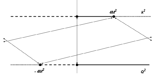
Figure 2: The boost (21) maps the dashed, solid, and dotted intervals of rest frame $k^{2}$ onto the dashed, solid, and dotted intervals of the Breit frame momentum transfer $Q^{2}$.

Evidently, the boost in Eq. (21) maps $G^{\mathrm{rest}}(k^{2}\to 4M^{2})~{}\to~{}G^{\mathrm{Breit}}(Q^{2}\to\infty)$. But, even though $G^{\mathrm{rest}}(4M^{2})$ may be very small, it generally does not vanish exactly. So, unless $n_{\mathrm{M}},n_{\mathrm{E}}\geq 2$, this shows up, of course, very drastically in the asymptotic behaviour, if the resulting form factors are divided by the standard dipole

$$G_{\mathrm{D}}(Q^{2})=1/(1+Q^{2}/0.71)^{2},$$ (22)

which is the common way to present the nucleon form factors and accounts for the proper asymptotic $Q^{2-2\nu}$ behaviour of an $\nu=3$ quark cluster. So it is vital for a comparison with experimentally determined form factors for $Q^{2}\gg M^{2}$ to employ a boost prescription which preserves at least the ’superconvergence’ property $Q^{2}G(Q^{2})\rightarrow 0$ for $Q^{2}\rightarrow\infty$. In accordance with an early suggestion by Mitra and Kumari Mitra ; Kelly we use $n_{\mathrm{M}}=n_{\mathrm{E}}=2$. In any case, the high-$Q^{2}$ behaviour is not a profound consequence of the model but simply reflects the boost prescription. There is no reason anyway, why low-energy effective models should provide any profound answer for the high-$Q^{2}$ limit. Note that the position of an eventual zero in $G_{\mathrm{E}}^{\mathrm{Breit}}(Q^{2})$ is not affected by the choice of the interpolating power $n_{\mathrm{E}}$, and the ratio $G_{\mathrm{E}}/G_{\mathrm{M}}$ is independent of the interpolating power, as long as $n_{\mathrm{M}}=n_{\mathrm{E}}$.

Figure 3: Magnetic and electric proton form factors $G_{\mathrm{M}}^{\mathrm{p}}/(\mu_{p}G_{\mathrm{D}})$ and $G_{\mathrm{E}}^{\mathrm{p}}/(G_{\mathrm{M}}^{\mathrm{p}}/\mu_{p})$ for the $\pi$-$\rho$-$\omega-$model with the set of parameters given in the text. The dotted line shows the result of Eq. (10) with $r_{B}=0.3$ fm. The abscissa shows $Q^{2}$(GeV/c)² on logarithmic scale. The experimental data are from Refs. Hoehler76 - Gayou02 .

Figure 4: The neutron electric form factor $G_{\mathrm{E}}^{\mathrm{n}}$ as obtained in the $\pi$-$\rho$-$\omega-$model with the set of parameters given in the text. The dotted line is the standard Galster parametrization $G_{\mathrm{E}}^{\mathrm{n}}=-\mu_{n}\tau/(1+5.6\tau)\cdot G_{\mathrm{D}}$ with $\tau=Q^{2}/(4M_{n}^{2})$. Experimental results for $G_{\mathrm{E}}^{\mathrm{n}}$ are mainly from more recent polarization data Ostrick99 - Plaster06 .

Figure 5: The magnetic neutron form factor (normalized to the standard dipole) $G_{\mathrm{M}}^{\mathrm{n}}/(\mu_{n}G_{\mathrm{D}})$ in the same model. Here the data are from Refs. Rock - Anderson .

V Results

To demonstrate the amount of agreement with experimental data that can be achieved within the framework of such models we present in Fig. 3 typical results from the $\pi$-$\rho$-$\omega-$model with essential parameters of the model fixed at their physical values: the pion decay constant $f_{\pi}=93$ MeV, the pion mass $m_{\pi}=138$ MeV, $\rho$-mass $m_{\rho}=770$ MeV, $\omega$-mass $m_{\omega}=783$ MeV, and the $\pi$-$\rho$-coupling constant at its physical KSRF-value $g_{\rho}=2.9$. As variable parameters remain the $\pi$-$\omega$ coupling constant $g_{\omega}$, and the $\omega$-photon coupling constant $g_{0}$. Due to the presence of dynamical $\rho$-mesons the strength $1/e^{2}$ of the fourth-order Skyrme term ${\cal L}^{(4)}$ should be reduced as compared to its standard value; it may even be omitted altogether. In addition to these three coupling constants, the high-$Q^{2}$ behaviour of the form factors is, of course, very sensitive to the effective kinematical mass $M$ which appears in the Lorentz-boost (19).

Altogether, while the general features are generic to the soliton model, we use in the following these four parameters $~{}g_{\omega}=1.4,~{}~{}g_{\omega}/g_{0}=0.75,~{}~{}e=7.5$, and $M=1.23$ GeV, for the fine-tuning of the proton form factors as shown in Fig. 3. Of course, these four parameters are not independent. Changes in the calculated form factors due to variations in one of these parameters may be compensated by suitable variations in the others for comparable quality of the fits. (For example, the agreement shown in Fig. 3 could also be obtained in a three-parameter fit without Skyrme term (i.e. $1/e^{2}=0$) with $g_{\omega}=2.4,~{}~{}g_{\omega}/g_{0}=0.7$, and $M=1.16$ GeV).

The absolute size of the neutron electric form factor $G_{\mathrm{E}}^{\mathrm{n}}$ is closely related to the choice of $g_{\omega}/g_{0}$. For the chosen set of parameters the maximum of $G_{\mathrm{E}}^{\mathrm{n}}$ exceeds the Galster parametrization by a factor of about 1.3 (cf. Fig. (4)). Correspondingly, the calculated values for the electric neutron square radii exceed the experimental value by about a factor of 2, and we found it difficult to lower them, for reasonable parametrizations within the $SU(2)$ framework. But otherwise the shape of $G_{\mathrm{E}}^{\mathrm{n}}$ follows the Galster parametrization rather well, with the maximum slightly shifted to lower $Q^{2}$. In the $SU(3)$-embedding of the Skyrme model the mixing coefficients for isoscalar, isovector, and kaonic contributions to the electromagnetic form factors cause a sizable reduction of the electric neutron form factor as compared to the $SU(2)$ scheme. The relevant coefficients are listed in Ref. Herbert for the case of exact flavor symmetry; when symmetry breaking is included, their numerical values reduce the square radius $\langle r^{2}\rangle^{n}_{\mathrm{E}}$ by a factor of about one-half as compared to $SU(2)$, while the results for the proton remain almost unaffected Herbert ; Hans . This cures the discrepancy for $G_{\mathrm{E}}^{\mathrm{n}}$ in Fig. (4) and for $\langle r^{2}\rangle^{n}_{\mathrm{E}}$ shown in Table 1. However, we are not aware of calculations of electromagnetic form factors for $Q^{2}>1$(GeV/c)² in the $SU(3)$-embedded Skyrme and vector meson model.

In Fig.5 we also present the resulting magnetic neutron form factor $G_{\mathrm{M}}^{\mathrm{n}}$, normalized to the standard dipole $G_{\mathrm{D}}$. For $Q^{2}\leq 1$(GeV/c)² the model result is in perfect agreement with the latest data Kelly04 (as quoted in Plaster06 ), Anderson . For $Q^{2}>1$(GeV/c)², however, the model prediction deviates substantially from the available older data Rock ; Lung . The ratio of the normalized proton and neutron magnetic form factors $G_{\mathrm{M}}^{\mathrm{n}}\mu_{p}/(G_{\mathrm{M}}^{\mathrm{p}}\mu_{n})$ is independent of the choice of the interpolating power $n_{\mathrm{M}}$ in the boost prescription. Therefore it would be desirable to compare directly with data for this ratio. Experimentally it is accessible from quasielastic scattering on deuterium with final state protons and neutrons detected. The generic scaling relation (5) predicts this ratio to be equal to one, $G_{\mathrm{M}}^{\mathrm{n}}\mu_{p}/(G_{\mathrm{M}}^{\mathrm{p}}\mu_{n})=1$, so deviations from this value indicate, how the function $B_{1}(r)$ which appears in $G^{1}_{\mathrm{M}}(k^{2})/\mu_{1}$ differs from $r^{2}B_{0}(r)$ in the specific model considered. Both, the Skyrme model and the $\pi$-$\rho$-$\omega-$model considered here, consistently predict this ratio to increase above 1 by up to 15% for $1<Q^{2}$(GeV/c)${}^{2}<10$. However, also in this case an $SU(3)$ embedding may change this prediction appreciably. The presently available data do not show such an increase for this ratio, in fact they indicate the opposite tendency. This conflict was already noticed in Refs. Ho ; Ho02 . Preliminary data from CLAS E94 apparently are compatible with $G_{\mathrm{M}}^{\mathrm{n}}/(\mu_{n}G_{\mathrm{D}})=1$ in the region $1<Q^{2}$(GeV/c)${}^{2}<4.5$ .

Table 1: Nucleon quadratic radii and magnetic moments as obtained from the chiral $\pi$-$\rho$-$\omega-$model, for the parameters given in the text. The experimental values are from Ref. Simon .

	$\langle r^{2}\rangle^{\mathrm{p}}_{\mathrm{E}}$	$\langle r^{2}\rangle^{\mathrm{p}}_{\mathrm{M}}$	$\langle r^{2}\rangle^{n}_{\mathrm{E}}$	$\langle r^{2}\rangle^{n}_{\mathrm{M}}$	$\mu_{p}$	$\mu_{n}$
Model	0.74	0.72	-0.24	0.76	1.82	-1.40
Exp.	0.77	0.74	-0.114	0.77	2.79	-1.91

In Table 1 we list quadratic radii and magnetic moments as they arise from the fit given above. Notoriously low are the magnetic moments. This fact is common to chiral soliton models and well known. Quantum corrections will partly be helpful in this respect (see Ref. MeiWall97 ), as they certainly are for the absolute value of the nucleon mass.

Of course, such models can be further extended. Addition of higher-order terms in the skyrmion lagrangian, explicit inclusion of axial vector mesons, non-minimal photon-coupling terms, provide more flexibility through additional parameters. Our point here, however, is to demonstrate that a minimal version as described above is capable of providing the characteristic features for both proton form factors and for the electric neutron form factor in remarkable detail. In fact, the unexpected decrease of $G_{\mathrm{E}}^{\mathrm{p}}$ was predicted by these models, and it will be interesting to compare with new data for $G_{\mathrm{M}}^{\mathrm{n}}$ concerning the conflict indicated in Fig. 5.

VI Extension to time-like $Q^{2}$

In the soliton rest frame the extension to time-like $k^{2}$ amounts to finding the spectral functions $\Gamma(\nu^{2})$ as Laplace transforms of the relevant densities $B(r)$, e.g. for the isoscalar electric case

$$rB_{0}(r)=\frac{1}{\pi^{2}}\int_{\nu_{0}^{2}}^{\infty}e^{-\nu r}\nu\Gamma_{0}(\nu^{2})d\nu,$$ (23)

and similarly for other cases. In soliton models the densities are obtained numerically on a spatial grid, therefore the spectral functions cannot be determined uniquely. Results will always depend on the choice of constraints which have to be imposed on possible solutions. But with reasonable choices it seems possible to stabilize the spectral functions in the regime from the 2- or 3-pion threshold to about two $\rho$-meson masses and distinguish continuous and discrete structures in this regime Ho .

We note (cf. Fig. (2)) that the transformation to the Breit frame (21) formally maps the rest frame form factors $G^{\mathrm{rest}}(k^{2})$ for the whole time-like regime $-\infty<k^{2}<0$ onto the Breit-frame form factors $G^{\mathrm{Breit}}(Q^{2})$ in the unphysical time-like regime up to the nucleon-antinucleon threshold $-4M^{2}<Q^{2}<0$. On the other hand, the physical time-like regime $-\infty<Q^{2}<-4M^{2}$ in the Breit frame is obtained as the image of the spacelike regime $4M^{2}<k^{2}<\infty$ of form factors in the rest frame. So the (real parts) of the Breit-frame form factors for time-like $Q^{2}$ beyond the nucleon-antinucleon threshold are formally fixed through Eq. (20). However, apart from the probably very limited validity of the boost prescription (20), we do not expect that the form factors in the soliton rest frame for $k^{2}>4M^{2}$ contain sufficiently reliable physical information. Specifically, oscillations which the rest frame form factors may show for $k^{2}\to\infty$, are sqeezed by the transformation (21) into the vicinity of the physical threshold $Q^{2}<-4M^{2}$. With $G^{\mathrm{rest}}(k^{2})\rightarrow 0$ for $k^{2}\rightarrow\infty$, the Breit-frame form factors are undetermined at threshold $Q^{2}\rightarrow-4M^{2}$.

Attempts to obtain form factors for time-like $Q^{2}$ from soliton-antisoliton configurations in the baryon number $B=0$ sector face the difficulty that in this sector the only stable classical configuration is the vacuum. So, any result will reflect the arbitrariness in the construction of nontrivial configurations.

Altogether we conclude, that presently we see no reliable way for extracting profound information about electromagnetic form factors in the physical time-like regime from soliton models.

VII Two-photon amplitudes in soliton models

The discrepancies between form factors extracted through the Rosenbluth separation from unpolarized elastic scattering data Qattan and ratios directly obtained from polarization transfer measurements Jones00 ; Gayou02 have lead to the difficult situation that two distinct methods to experimentally determine fundamental nucleon properties yield inconsistent results Arrington . As a possible remedy, the theoretical focus has shifted to two-photon amplitudes which enter the unpolarized cross section and polarization variables in different ways. Two-photon exchange diagrams involve the full response of the nucleon to doubly virtual Compton scattering and therefore rely heavily on specific nucleon models. Simple box diagrams which iterate the single-photon exchange, require virtual intermediate nucleons and resonances with unknown off-shell form factors. They have been analysed with various assumptions for the intermediate states and have been found helpful for a partial reduction of the discrepancies 2Photbox ; Carlson .

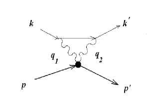
Figure 6: Electron-nucleon scattering $2\gamma$-exchange amplitude with local $2\gamma$-soliton vertex with momentum transfer $q=q_{1}-q_{2}=k-k^{\prime}=p^{\prime}-p.$

It is interesting to note that, in addition to box diagrams, soliton models contain 2$\gamma$-exchange contributions where the two virtual photons interact with the pion cloud of the baryon at local two-photon vertices. Products of covariant derivatives

$$D_{\mu}U=\partial_{\mu}U+i[\hat{Q},U]A_{\mu}$$ (24)

which appear in all terms of the derivative expansion after gauging the chiral fields with the electric charge $\hat{Q}$, naturally produce these local two-photon couplings. The simplest ones originate from the quadratic nonlinear $\sigma$-term and from the gauged Wess-Zumino anomalous action

$${\cal L}^{(2\gamma)}_{nl\sigma}=-\frac{f_{\pi}^{2}}{4}A_{\mu}A^{\mu}2{\mbox{t}r}(\hat{Q}U\hat{Q}U^{\dagger}-\hat{Q}^{2}),$$ (25)

$${\cal L}^{(2\gamma)}_{W\!Z}=i\frac{N_{c}}{48\pi^{2}}\varepsilon^{\mu\nu\varrho\sigma}(\partial_{\mu}A_{\nu})A_{\varrho}{\mbox{t}r}\left(\hat{Q}\partial_{\sigma}U\hat{Q}U^{\dagger}-\hat{Q}U\hat{Q}\partial_{\sigma}U^{\dagger}+2\hat{Q}^{2}(U^{\dagger}\partial_{\sigma}U-U\partial_{\sigma}U^{\dagger})\right).$$ (26)

After quantization of the collective coordinates the matrix elements of these $2\gamma$-vertices sandwiched between incoming and outgoing nucleon states are obtained, without additional parameters, with form factors fixed through the soliton profiles. Then the interference terms with the single-photon-exchange amplitudes for the unpolarized elastic cross section can be evaluated. It turns out that the contribution from ${\cal L}^{(2\gamma)}_{nl\sigma}$ interferes only with the electric part of the 1-photon-exchange Born term and vanishes after spin averaging. On the other hand, the scattering amplitude following from ${\cal L}^{(2\gamma)}_{W\!Z}$ interferes only with the magnetic part of the Born amplitude, so that apart from kinematical factors the unpolarized elastic electron-nucleon cross section has the general structure

$$\frac{d\sigma}{d\Omega}\propto\left(G_{\mathrm{M}}^{2}(Q^{2})+\frac{\epsilon}{\tau}G_{\mathrm{E}}^{2}(Q^{2})+\nu(1-\epsilon)G_{\mathrm{M}}(Q^{2})F^{(2\gamma)}_{W\!Z}(Q^{2})\right)$$ (27)

with Lorentz invariants $\tau=Q^{2}/(4M^{2})$, and

$$\nu=\frac{1}{4}(k+k^{\prime})\cdot(p+p^{\prime})=\sqrt{\tau(1+\tau)\frac{1+\epsilon}{1-\epsilon}}~{}.$$ (28)

The form factor $F^{(2\gamma)}_{W\!Z}$ is of the order of the electromagnetic coupling constant $\alpha$, and involves a loop integral and Fourier transforms of soliton profiles. Due to its origin from the Wess-Zumino action, it is parameter free. The possibility to obtain parameter free information about the influence of two-photon exchange contributions, makes this scheme very attractive. However, it should be mentioned that the infinite part of the loop integral requires a counterterm which has to be fixed by other experimental input. This program has been performed in Ref.Kuhn . The corrections obtained have been found to reduce the observed discrepancies, with an absolute size, however, which by itself is also not sufficient to resolve the problem. It has to be supplemented by iterated single-photon exchange.

The $\epsilon$-dependence through $\sqrt{(1+\epsilon)/(1-\epsilon)}$ as contained in $\nu$ is a general symmetry and consistency requirement for the two-photon interaction Rekalo . There is, however, experimental evidence that within the present error limits the unpolarized elastic cross section is consistent with a linear $\epsilon$-dependence Chen ; Tomasi . This still allows to extract via Rosenbluth separation, effective electric and magnetic form factors which then comprise also the sum of all relevant 2$\gamma$-contributions. Their ratios may differ appreciably from ratios of the single-photon-exchange form factors $G^{\mathrm{p}}_{\mathrm{E}}/G^{\mathrm{p}}_{\mathrm{M}}$ as extracted from polarization transfer data, which are believed to remain mostly unaffected by 2$\gamma$-contributions Carlson . Although at present the situation is not yet fully understood, there is strong evidence that 2$\gamma$-exchange effects may in fact account for most of the observed differences ArMelTj , and electromagnetic form factors remain the challenging testing ground for models of the nucleon.

The fact that the unexpected results of the polarization transfer experiments follow as generic consequence from soliton models; that within a minimal specific model form factors can be reproduced in detail; and that, in addition to the usual box diagrams, standard gauging provides a new class of radiative corrections with local 2$\gamma$-nucleon coupling; all of this once again underlines the strength of the soliton approach to baryons.

References

- (1) G. Holzwarth, Z. Phys. A356 (1996) 339; Proc. 6th Int. Symp. Meson-Nucleon Phys., Newsletter 10 (1995) 103.
- (2) E. Braaten, S.M. Tse and C. Willcox, Phys. Rev. D34 (1986) 1482; Phys. Rev. Lett. 56 (1986) 2008.
-
(3)
O. Kaymakcalan and J. Schechter, Phys. Rev. D31 (1985) 1109;
M. Bando, T. Kugo, S Uehara, K. Yamawaki, and T. Yanagida, Phys. Rev. Lett. 54 (1985) 1215. -
(4)
U.G. Meissner, N. Kaiser and W. Weise, Nucl. Phys. A466 (1987)
685;
U.G. Meissner, Phys. Reports 161 (1988) 213. - (5) B. Schwesinger, H.Weigel, G.Holzwarth, and A. Hayashi, Phys. Reports 173 (1989) 173.
- (6) F. Meier, in: Baryons as Skyrme solitons, ed. G. Holzwarth (World Scientific, Singapore 1993), 159.
- (7) V.A. Matveev, R.M. Muradyan, and A.N. Tavkhelidze, Lett. Nuovo Cim. 7 (1973) 719.
- (8) A.L. Licht and A. Pagnamenta, Phys. Rev. D2 (1976) 1150 ; and 1156.
- (9) X. Ji, Phys. Lett. B254 (1991) 456.
- (10) A. N. Mitra and I. Kumari, Phys. Rev. D15 (1977) 261.
- (11) J.J. Kelly, Phys. Rev. C66 (2002) 065203.
- (12) H. Weigel, Chiral Soliton Models for Baryons, Lect. Notes Phys. 743 (Springer, Berlin Heidelberg 2008), p.118.
- (13) H. Walliser, private communication.
- (14) G. Höhler et al., Nucl. Phys. B114 (1976) 505.
- (15) A.F. Sill et al., Phys. Rev. D48 (1993) 29.
- (16) L. Andivahis et al., Phys. Rev. D50 (1994) 5491.
- (17) R.C. Walker et al., Phys. Rev. D49 (1994) 5671.
- (18) M. K. Jones et al., Phys. Rev. Lett. 84 (2000) 1398.
- (19) O. Gayou et al., Phys. Rev. Lett. 88 (2002) 092301.
- (20) M. Ostrick et al., Phys. Rev. Lett. 83 (1999) 276.
- (21) M. Meyerhoff et al., Phys. Lett. B327 (1994) 201.
- (22) J. Becker et al., Eur. Phys. J. A6 (1999) 329.
- (23) D. Rohe et al., Phys. Rev. Lett. 83 (1999) 4257.
- (24) R. Schiavilla, and I. Sick, Phys. Rev. C64 (2001) 041002-1.
- (25) R. Glazier et al., Eur.Phys.J. A24 (2005) 101.
-
(26)
B. Plaster et al. [E93-038 Collaboration], Phys. Rev. C73 (2006) 025205;
R. Madey et al., Phys. Rev. Lett. 91 (2003) 122002. - (27) S. Rock et al., Phys. Rev. Lett. 49 (1982) 1139.
- (28) A. Lung et al., Phys. Rev. Lett. 70 (1993) 718.
- (29) H. Anklin et al., Phys. Lett. B336 (1994) 313.
- (30) H. Anklin et al., Phys. Lett. B428 (1998) 248.
- (31) G. Kubon, H. Anklin et al., Phys. Lett. B524 (2002) 26.
- (32) J. J. Kelly, Phys.Rev. C70 (2004) 068202.
-
(33)
B. Anderson et al. [E95-001 Collaboration], Phys.Rev. C75 (2007) 034003;
W. Xu et al., Phys. Rev. Lett. 85 (2000) 2900; Phys. Rev. C67 (2003) 012201. - (34) G. Holzwarth, [arXiv:hep-ph/0201138].
- (35) W. K. Brooks and J. D. Lachniet [CLAS E94-017 Collaboration], Nucl.Phys. A755 (2005) 261.
- (36) G. Simon et al., Z. Naturforsch. 35A (1980) 1.
- (37) F. Meier and H. Walliser, Phys. Reports 289 (1997) 383.
-
(38)
M. E. Christy et al. [E94110 Collaboration], Phys. Rev. C70 (2004) 015206;
I. A. Qattan et al., Phys. Rev. Lett. 94 (2005) 142301 . -
(39)
J. Arrington, Phys. Rev. C68 (2003) 034325; Phys. Rev. C69 (2004)
022201; Phys. Rev. C71 (2005) 015202;
H. Gao, Int. J. Mod. Phys. A20 (2005) 1595. -
(40)
P. A. M. Guichon and M. Vanderhaeghen, Phys. Rev. Lett. 91 (2003) 142303;
P. G. Blunden, W. Melnitchouk, and J. A. Tjon, Phys. Rev. Lett. 91 (2003) 142304; Phys. Rev. C72 (2005) 034612;
Y. C. Chen et al., Phys. Rev. Lett. 93 (2004) 122301;
A. V. Afanasev et al., Phys. Rev. D 72 (2005) 013008;
S. Kondratyuk et al., Phys. Rev. Lett. 95 (2005) 172503;
P. Jain et al., arXiv:hep-ph/0606149;
D. Borisyuk and A. Kobushkin, Phys. Rev. C74 (2006) 065203;
C. F. Perdrisat, V. Punjabi, and M. Vanderhaeghen, Prog. Part. Nucl. Phys. 59 (2007) 694. - (41) C. E. Carlson and M. Vanderhaeghen, Annu. Rev. Nucl. Part. Sci. 57 (2007) 171;
- (42) M. Kuhn and H. Weigel, arXiv:0804.3334 [nucl-th], to be publ. in Eur. Phys. J. A .
- (43) M. P. Rekalo and E. Tomasi-Gustafsson, Eur. Phys. J. A22 (2004) 331; Nucl. Phys. A742 (2004) 322.
-
(44)
E. Tomasi-Gustafsson and G. I. Gakh, Phys. Rev. C72 (2005) 015209;
V. Tvaskis et al., Phys. Rev. C73 (2006) 025206. - (45) Y. C. Chen, C.W. Kao and S. N. Yang, Phys. Lett. B652 (2007) 269.
- (46) J.Arrington, W. Melnitchouk, and J.A.Tjon, Phys. Rev. C76 (2007) 035205.