Faculty of Physics and Astronomy

University of Heidelberg

Diploma thesis
in Physics
submitted by
Korinna Zapp
born in Eckernförde
2005

The Soft Scattering Contribution to Jet Quenching in a Quark-Gluon Plasma and General Properties of
Partonic Energy Loss

This diploma thesis has been carried out by Korinna Zapp at the
Institute of Physics
under the supervision of
Prof. Dr. Johanna Stachel

Der Beitrag von weicher Streuung zum Jet Quenching in einem Quark-Gluon Plasma und allgemeine Eigenschaften des Energieverlusts von Partonen

Ausgehend von der Beobachtung, dass weiche Streuungen eines hart gestreuten Partons am Farbladung tragenden Protonüberrest in Proton-Proton Kollisionen eine wichtige Rolle spielen, wurde ein ähnliches Modell für weiche Streuung in einem Quark-Gluon Plasma konstruiert und als Monte Carlo Generator implementiert. Die hauptsächliche Frage war, inwieweit diese weichen Streuungen zum Energieverlust beitragen können, den ein hochenergetisches Parton erleidet, wenn es ein Quark-Gluon Plasma durchquert. Das Ergebnis war, dass sie bis zu 50% des beobachteten Energieverlusts erklären können.

Außerdem wurde die Frage untersucht, was man von heute verfügbaren Daten über die allgemeinen Eigenschaften des Energieverlusts von Partonen erfahren kann. Dazu wurde ein Monte Carlo Modell benutzt, das zwar die volle Simulation des Quark-Gluon Plasmas beinhaltet aber für den Energieverlust einen allgemeineren Ansatz verwendet. Dadurch wird es möglich verschiedene Szenarien wie kohärente Gluonbremsstrahlung, Streuung etc. nachzubilden. Leider stellte sich heraus, dass es sehr schwierig ist die verschiedenen Möglichkeiten zu unterscheiden, sodass zum jetzigen Zeitpunkt keine eindeutige Entscheidung zugunsten der einen oder anderen möglich ist.

The Soft Scattering Contribution to Jet Quenching in a Quark-Gluon Plasma and General Properties of Partonic Energy Loss

Starting from the observation that soft rescattering of hard scattered partons from the colour charged remnant plays an important role in proton-proton collisions a similar model for soft scatterings in a quark-gluon plasma was constructed and implemented as a Monte Carlo event generator. The main emphasis was put on the question to what extend these soft scatterings can contribute to the energy loss that an energetic parton suffers, when it traverses a quark-gluon plasma. It was found that the soft scattering can account for up to 50% of the observed energy loss.

Furthermore, it was investigated what information present data reveal about the general features of partonic energy loss. This study was carried out with a Monte Carlo model that includes the full simulation of the quark-gluon plasma but uses a more general ansatz for the energy loss which makes it possible to emulate different scenarios like coherent gluon bremsstrahlung, scattering etc. Unfortunately, it turned out that it is difficult to differentiate between them so that at present no clear decision in favour of one or the other is possible.

Contents

1. 0 Introduction
2. 1 QCD for Beginners
   1. 1 Introduction
   2. 2 Structure of the proton and parton showers
   3. 3 Fragmentation
      1. 1 String Fragmentation
      2. 2 Independent Fragmentation
3. 2 Hunting the Quark Gluon Plasma
   1. 1 QCD Predictions
   2. 2 Models
   3. 3 Observables
4. 3 Jet Quenching
5. 4 Basics of Heavy Ion Physics
   1. 1 Glauber models
   2. 2 Quantum Statistics of an Ideal Quark-Gluon Gas
   3. 3 The Bjorken Model
   4. 4 Azimuthal Anisotropy
   5. 5 Cronin effect
   6. 6 Radiative Energy Loss
6. 5 Experimental Results
   1. 1 AGS and SPS
   2. 2 RHIC
      1. 1 Suppression of high-$p_{\perp}$ Hadrons
      2. 2 Disappearance of Back-to-Back Hadron Correlations
      3. 3 Correlation with the Reaction Plane
      4. 4 Other Observables
7. 6 Comparison of Identified Particle Spectra from SPS and RHIC
8. 7 Monte Carlo Techniques
9. 8 Soft Colour Interactions
10. 9 The Soft Colour Interaction Jet Quenching Model
    1. 1 Description of the Model
       1. 1 Geometry
       2. 2 Cronin Effect
       3. 3 Model of the QGP: Energy Density Distribution, EOS and Evolution
       4. 4 Energy Loss
       5. 5 Hadronisation
       6. 6 Model Parameters
    2. 2 Results
       1. 1 Cronin Effect
       2. 2 Nuclear Modification Factor
       3. 3 Azimuthal Correlation
    3. 3 Discussion
11. 10 Exploring General Properties of Partonic Energy Loss
    1. 1 Motivation
    2. 2 Energy Loss in the Toymodel
    3. 3 Results
    4. 4 Summary and Discussion
12. 11 Conclusions and Outlook
13. 12 Fit Parameters for Identified Particle Spectra
14. 13 Complete Results from the Toymodel

Chapter 0 Introduction

The quark-gluon plasma (QGP) is a state of deconfined quarks and gluons and restored chiral symmetry predicted by Quantum Chromodynamics (QCD), the theory of the strong interactions. It is expected to be formed at very high energy densities. It presumably existed in the early universe and can possibly still today be found in some kinds of neutron stars or other exotic objects. Great efforts are being made to produce the QGP in the laboratory by means of heavy ion collisions. This is the only possibility to reach high enough energy densities in man-made experiments. The price that has to be paid is that the QGP – if it is formed at all – has a very short lifetime because of rapid expansion and thus cooling of the system.

The detection and study of the QGP is a highly non-trivial task that has kept both experimentalists and theorists busy for many years and is still far from completed. The observables can be grouped into soft and hard probes. The hard probes are sensitive to the very early stage of the collision whereas the soft ones probe the latest stage. Hard observables such as jet quenching (suppression of particles with high transverse momentum) have only recently become accessible with the Relativistic Heavy Ion Collider (RHIC) in Brookhaven, where data taking started in 2000. They are considered an adequate tool for investigating the properties of the medium created in the collisions wherefore sometimes the term ”jet tomography” is used. For the proof of QGP formation on the other hand other observables like thermal and chemical equilibration are more suited.

Most of the phenomena connected to heavy ion collisions and QGP formation and its evolution belong to the non-perturbative regime of QCD where it is very difficult to derive a quantitative description from first principles. Thus models of different scenarios have to be constructed and the results compared to data in order to learn something about the physics. This is often a laborious business and it is in the majority of cases not possible to obtain clear cut conclusions.

In this thesis a new model for the jet quenching is presented and compared to data. It is built on partonic energy loss due to soft colour interactions. The starting point was the Soft Colour Interaction (SCI) model [1] that successfully describes a wealth of data mainly on deep inelastic scattering and diffraction. The SCI model has been extended in order to be applicable for the jet quenching phenomena.

There is no perfect model for the jet quenching, so this new model can hopefully help to gain a better understanding of the effects in QGP and soft physics in general. The SCI jet quenching model is implemented as a Monte Carlo event generator which has the advantage that the processes can be simulated and studied in great detail.

A second issue of this thesis are the general properties of the energy loss mechanism. Different theoretical approaches lead to quite different behaviours. The idea is to see what presently available data reveal about the main features of the sought energy loss mechanism without having a detailed model. This information may then help to get to the right description in the end.

In the first part of this report a short overview of QCD, the search for the QGP, jet quenching as a possible signature of the QGP and a few basics of heavy ion physics is given. There is also a discussion of experimental results with the main focus on jet quenching. After a brief introduction to Monte Carlo methods and the SCI model the new jet quenching model is described and compared to data in more detail. In the following section an investigation of general features of energy loss in the QGP is carried out with the help of an adjusted Monte Carlo model.

Chapter 1 QCD for Beginners

This section gives an introduction to the basics of QCD and some topics that are relevant for this study. A more systematic and detailed discussion can be found in [2, 3] or other standard books.

1 Introduction

Quantum Chromodynamics (QCD) is the theory of the strong interaction. It describes the interaction of quarks via exchange of gluons. There are the six quarks called down ($d$), up ($u$), strange ($s$), charm ($c$), bottom ($b$) and top ($t$) which are fermions and the massless gluons which are bosons. The relevant charge, which is the source of the field, is called colour and the three states are labelled red ($r$), blue ($b$) and green ($g$). Quarks come as colour triplets, which means that a particular quark can carry any of the three colours. The antiquarks form the corresponding antitriplet (i.e. they carry the anticolours $\bar{r}$, $\bar{b}$ and $\bar{g}$). Quarks cannot be observed as free particles but are always confined into hadrons, which are colour neutral objects. A colour neutral combination is also called a singlet. There are at least two possible neutral colour combinations: a colour and its matching anticolour (giving rise to mesons that are composed of one quark and one antiquark), or the three (anti)colours (leading to (anti)baryons that consist of three (anti)quarks). There is also a possibility to combine two quarks, but it is not clear to what extend these diquarks are bound states. Nevertheless, they can be very useful, e.g. for the treatment of remnants as will be discussed later. The combination of two triplet charges gives an antitriplet (or a sextet, but this is not interesting in this context), two antitriplets form a triplet.

The gluons are also colour charged, but unlike the quarks they carry octet charges which can be viewed as the combination of a colour and an anticolour (the combination of colour and anticolour gives a singlet and an octet). The name octet already indicates that it contains eight states. The naively expected nineth gluon does not occur because as a colour singlet combination it does not correspond to an interaction. The fact that the gluons carry colour charge gives rise to the gluon self-interaction, which means that gluons can directly couple to each other.

The coupling strength of the strong interaction $\alpha_{s}$ is not constant but depends on the momentum transfer such that it increases with decreasing energy scale. Therefore processes involving large momentum transfers can be treated analytically since it is possible to make a perturbative expansion in powers of $\alpha_{s}$. In regimes with small energy scales, where the coupling is large, pertubation theory is not applicable and other ways to treat these problems have to be found. One possibility is to solve the equations numerically, which has its own problems. This task is highly non-trivial and to a great extent limited by the available computing power. In many cases one has to rely on phenomenological models that describe the observed phenomena without having a firm theoretical basis.

2 Structure of the proton and parton showers

The proton is a baryon built of three valence quarks (two $u$- and one $d$-quark) which carry its electric charge and baryon number. In addition, there are also gluons and sea quarks that are fluctuations of gluons into quark-antiquark pairs. The quarks carry approximately 50% of the proton’s energy-momentum, the other half is carried by the gluons.

.......................................................................................................................................................................................................................................................................................................................................................................................................................................................................................................................................................................................................................................................................................................................................................................................................................................................................................................................................................................................................................................................................................................................................................................$p$.....................................................................................................................................................................................................................................  ......................................................   ..................................................................................................................................................................................................................   ......................................................  $q$$k$$k^{\prime}$   

Figure 1: Inelastic lepton-proton scattering via exchange of a virtual photon

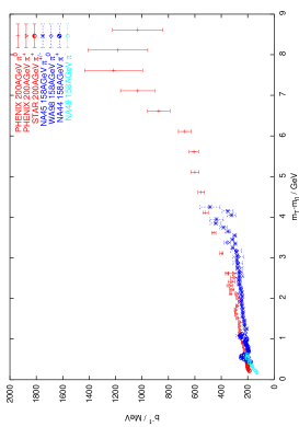
Figure 1: Fit parameters for the pion spectra

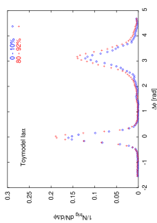
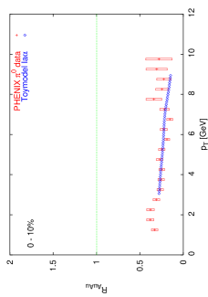
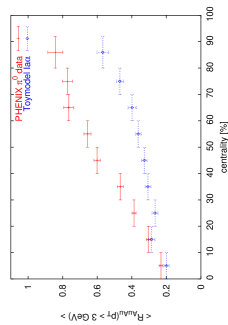
Figure 1: Results for the Toymodel I a $\alpha$ with $\Delta E\propto N_{g}E$ and homogeneous energy density distribution

The best way to investigate the structure of the proton is in lepton-proton scattering via photon exchange (Fig. 1). The standard variables are

$$Q^{2} = -q^{2}$$ (1)

$$x = \frac{-q^{2}}{2p\cdot q}$$ (2)

$$y = \frac{q\cdot p}{k\cdot p}$$ (3)

where $p$, $q$ and $k$ are the proton’s, the photon’s and the lepton’s four-momenta, respectively ($k$ refers to the initial and $k^{\prime}$ to the final vector).

At small momentum transfers $Q^{2}$ the photon interacts with the proton as a whole, but at higher $Q^{2}$ the structure of the proton can be resolved. The momentum transfer can be viewed as the resolution: With a bigger $Q^{2}$ smaller structures can be resolved (the resolution is $d\sim 0.2\,\mathrm{fm}/\sqrt{Q^{2}}[\mathrm{GeV}]$). The cross section can be written as

$$\frac{\mathrm{d}^{2}\sigma}{\mathrm{d}Q^{2}\mathrm{d}x}=\frac{4\pi}{xQ^{4}}((1-y)F_{2}+xy^{2}F_{1})$$ (4)

where the structure functions $F_{i}(x,Q^{2})$ parametrise the proton structure. They are approximately independent of $Q^{2}$ (Bjorken scaling) which implies that the photon interacts with quasi-free pointlike constituents (partons) of the proton. In the frame where the proton has infinite momentum, $x$ can be interpreted as the limit of the fraction of the proton’s momentum carried by the parton. The structure function $F_{2}$ can to lowest order be written as

$$F_{2}(x,Q^{2})=\sum_{a}e_{a}^{2}xf_{a}(x,Q^{2})$$ (5)

where $a$ runs over all flavours and antiflavours, $e_{a}$ is the electric charge of the respective quark or antiquark and $f_{a}(x,Q^{2})$ is the probability of finding a quark of flavour $a$ carrying the momentum fraction $x$ inside the proton when probing with momentum transfer $Q^{2}$. The $f_{a}$ are called parton distribution functions (pdf’s), they include the contributions from both the valence and the sea quarks. Scattering of the lepton from gluons is not possible since the gluons do not carry electric charge.

$F_{1}$ is connected to $F_{2}$ via the Callan-Gross relation

$$F_{2}=2xF_{1}$$ (6)

The $Q^{2}$ dependence of the parton distribution arises from the fact that the (anti)quark may have radiated gluons (initial state radiation) before it was actually struck by the photon. The $Q^{2}$ dependence can be calculated in pertubation theory and is governed by the DGLAP evolution equations

$$\frac{\partial f_{q}(x,Q^{2})}{\partial\ln Q^{2}}=\frac{\alpha_{s}(Q^{2})}{2\pi}\int\limits_{x}^{1}\frac{\mathrm{d}y}{y}\ \left[P_{qq}\left(\frac{x}{y}\right)f_{q}(y,Q^{2})+P_{qg}\left(\frac{x}{y}\right)f_{g}(y,Q^{2})\right]$$ (7)

$$\frac{\partial f_{g}(x,Q^{2})}{\partial\ln Q^{2}}=\frac{\alpha_{s}(Q^{2})}{2\pi}\int\limits_{x}^{1}\frac{\mathrm{d}y}{y}\ \left[P_{gq}\left(\frac{x}{y}\right)f_{q}(y,Q^{2})+P_{gg}\left(\frac{x}{y}\right)f_{g}(y,Q^{2})\right]$$ (8)

where $f_{q}$ and $f_{g}$ are the quark and gluon pdf’s, respectively. The $P_{ij}$ are called splitting functions and describe the evolution of a parton $j$ into a parton $i$ carrying the energy fraction $z=x/y$ of the original parton. $P_{qq}$ for instance describes the radiation of a gluon from a quark where the quark keeps the energy fraction $z$; $P_{gq}$ describes the same situation when the gluon gets the fraction $z$ and the quark obtaines $1-z$.

There are similar equations for gluon radiation after the photon-parton scattering (final state radiation). The gluons tend to be emitted with small angles relative to the (anti)quark. The branching processes can explicitly be simulated using parton showers.

In contrast to the $Q^{2}$ dependence, the $x$ dependence of the pdf’s has to be parametrised and fitted to data. There are of course parton densities for all hadrons, it is common to write $f_{a/h}$ for the pdf of the parton $a$ in hadron $h$.

For (perturbatively hard) hadron-hadron processes any inclusive cross section can be factorised into the form

$$\sigma(p_{1},p_{2})=\sum_{a,b}\int\!\mathrm{d}x_{1}\,\mathrm{d}x_{2}\ f_{a}(x_{1},\mu^{2})f_{b}(x_{2},\mu^{2})\hat{\sigma}_{a,b}(x_{1}p_{1},x_{2}p_{2};Q^{2}/\mu^{2})$$ (9)

where $\hat{\sigma}_{a,b}$ is the parton level cross section for the parton species $a,b$ and $\mu^{2}$ is an arbitrary factorisation scale separating the hard from the soft regime. (It is a factorisation of the process in pdf’s and the parton-parton process described by $\hat{\sigma}_{a,b}$.)

3 Fragmentation

Quarks and gluons cannot be observed as free particles but are confined in colour neutral hadrons. The process of hadron formation from partons (quarks and gluons) falls into the domain of non-perturbative QCD and it has not been possible to derive it from first principles (it might become possible with lattice QCD). Nevertheless, a profound understanding of these mechanisms is of great importance for all kinds of activities in high energy physics, where the dynamics on the parton level has to be deduced from the observed hadronic final state.

There are basically three models: string fragmentation, independent fragmentation and cluster fragmentation. The main ideas of the Lund string model [4] and the independent fragmentation ([5], see also [6] for an overview) will be reviewed briefly here.

1 String Fragmentation

            ...................................................................................................................................................................................................................................................................................................................   ............................  ............................................  ..................................................................  ............................................  .................................................................................................................  .................................................................................................................  ..................................................................................................................  ............................................................................................................      ................................................................  ............................................    ................................   ....................................................p........................................................................................................................................................................................................$q$$qq$p$q$$qq$          

Figure 2: Quark-quark scattering via gluon exchange as an example of inelastic pp scattering with the resulting colour field topology represented by strings (dotted lines)

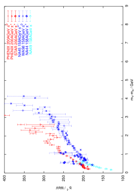
Figure 2: Enlarged low $p_{\perp}$ region of the above pion results

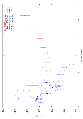
Figure 3: Fit parameters for the feed-down corrected proton spectra

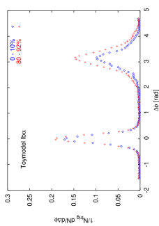
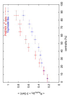
Figure 2: Results for the Toymodel I b $\alpha$ with $\Delta E\propto N_{g}^{2}E$ and homogeneous energy density distribution

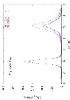
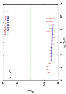
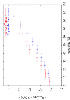
Figure 3: Results for the Toymodel II a $\alpha$ with $\Delta E\propto N_{g}E$ and inhomogeneous energy density distribution

The jet production from a hard quark-quark scattering in a proton-proton collision can serve as a simple example for the fragmentation of a quark. In this interaction the protons are broken apart: The two quarks are scattered to large angles and the remnants (in this case diquarks) continue in the beam directions. The incoming protons are colour singlets, after the scattering the (colour-)charged constituents can again be grouped into two colour neutral systems (Fig. 2). A field stretches between a colour charge (triplet charge) and its matching anticolour (antitriplet, in this case the diquark). Due to the gluon self-interaction the field does not extend transversly in space but can be viewed as a colour flux tube with transverse size $\sim 1\,\mathrm{fm}$. The potential rises linearly with the distance between the charges and at some point it becomes possible to form a new quark-antiquark pair from the field energy. This process is sketched in Figure 3.

  ...............................  ....  .....  .....                ...............................  ....    .....  .....              .............................................    .....      .....          ........................  ......    .....    .....            .......................  ...  ....      .....              ..................................  ....    .....                ..............................................      ..........            ...............................  ....    .....  .....              ........................................  ....  .....      ....          .......................  ...    ....    .....              .....................  ...  ...  ....      .....            .............................................      ..........              ...............................  ....  .....  .....                ...............................  ....    .....  .....              ..............................................    .....      .....          ........................  ......    .....    .....            .......................  ...  ....      .....              ..................................  ....    .....                ..............................................      ..........            ...............................  ....    .....  .....              ........................................  ....  .....      ....          .......................  ...    ....    .....              .....................  ...  ...  ....      .....            ..............................................      ..........            .......................  ......  ....            ....          ...........................................          .....  ....        ..............................  ....            ....          .............................................          .....    ...      .......................  ...    ....    .....              ......................  ...  ...  ....      .....            ............................  ...  ....          ....          ............................................          .....  ....        (c)...............................  ....            ....          ......................................  ....          .....    ...      ........................  ......    .....    .....            .......................  ...  ....      .....                    ...................................................................................................................................................................................    ........................................................  ..................................  ....    .....                ...............................................      ..........            ...............................  ....            ....          .....................................  ........      .....    ....        .......................  ...    ....    .....              .....................  ...  ...  ....      .....            ..............................  ....                        ...............................................      ..........            ...............................  ....            ....          .......................  ......    .....    .....            .......................  ...  ....      .....              .........................................  ....      .....    ....        $q$$qq$$q$$qq$$q$$qq$$\bar{q}$$q$(a)(b)   

Figure 3: Creation of a $q\bar{q}$ pair from the field energy during the separation of a quark ($q$) and a diquark ($qq$)

In the Lund model the colour flux tube is idealised to a one-dimensional massless relativistic string with energy density $\kappa\simeq 1\,\mathrm{GeV/fm}$. A newly produced $q\bar{q}$ pair breaks the string into two independent parts. The creation of a $q\bar{q}$ pair is described as a quantum mechanical tunneling process so that the probability becomes [4]

$$P\sim\exp\left(-\frac{\pi m_{\perp}^{2}}{\kappa}\right)=\exp\left(-\frac{\pi m^{2}}{\kappa}\right)\exp\left(-\frac{\pi p_{\perp}^{2}}{\kappa}\right)$$ (10)

This leads to a Gaussian distribution of the two transverse components of the produced (anti)quark’s momentum ($p_{x}$ and $p_{y}$ if the string is stretched along the $z$-axis). The transverse momentum is compensated when the string breaks between the created quark and the antiquark. Equation 10 shows also that the creation of heavy flavours is suppressed so that charm, bottom and top quarks are not expected to be produced. Since the quark masses are not well defined in this context the suppression of strangeness relative to $u$ (or $d$) quarks is left as a parameter with $\gamma_{s}=\frac{s\bar{s}}{u\bar{u}}\sim 0.3$.

It is assumed that a meson is formed when the invariant mass of a string piece becomes small. Its $p_{\perp}$ is given by the sum of the transverse momenta of the string endpoints, which also fix the flavour composition. The spin of the meson is chosen to be either 0 or 1 according to a suitable probability, orbital excitations are expected to be rare and are therefore excluded in the default Lund model.

The different break-ups of the string are assumed to be independent of each other. It is therefore possible to start at one end of the string, make a break-up and be left with a meson and a shorter string. The procedure can be iterated until the available energy is used up (the termination requires some extra treatment that will not be discussed here). Let us consider the string in the c.m. frame of the quark and the diquark with the quark moving in the $+z$-direction and start with the fragmentation from the quark end. The first step is to choose the flavour, spin and transverse momentum of the created $q\bar{q}$ pair as described above. The identity and transverse mass of the meson are then fixed and only the longitudinal momentum (or the energy) remains to be determined. This is done by assigning the meson a fraction $z$ of the available $E+p_{z}$. What is left to the new string is [4]

$$(E+p_{z})_{\mathrm{new}} = (1-z)(E+p_{z})_{\mathrm{old}}$$ (11)

$$(E-p_{z})_{\mathrm{new}} = (E-p_{z})_{\mathrm{old}}-\frac{m_{\perp}^{2}}{z(E+p_{z})_{\mathrm{old}}}$$ (12)

The values of $z$ are distributed according to a probability distribution $f(z)$. The constraint that the result should be independent of the choice from which end to start leads to the ’Lund symmetric fragmentation function’

$$f(z)\propto z^{-1}(1-z)^{a}\exp\left(-\frac{bm_{\perp}^{2}}{z}\right)$$ (13)

One important point is that the hadron that contains the end-(di)quark of the string will typically have the highest momentum in the ensemble. It should further be noted that in the lab system it is the slowest hadrons that are formed first, because all particles have a formation time of $\sim 1\,\mathrm{fm}$ in their rest frame. The difference in formation time in the lab frame is a boost effect. This ordering is frame dependent and therefore not important for the fragmentation algorithm, which is Lorentz invariant.

            ...........................................................................................................................................................................................................................................................................................................................................................................................................................   ............................  ............................................  ..................................................................  ............................................  .................................................................................................................  .................................................................................................................  ..................................................................................................................  ............................................................................................................      ................................................................  ............................................    ................................   .................   .......................  ................   ............................      ............................   ......................  ................   ............................      ................................   ..........................................   ............................      ....................................   ..........................................   ..............................  ..................................   ........................  ..................   ..............................  ..................p.................   ........................  ..................   ............................      ............................   ........................  ..................   ............................      ...............................................................................   ............................      ....................................   ..........................................   ..............................  ..................................   ........................  ..................   ..............................  ..................................   ...........................  ................   ............................      ............................   ..........................................     ............................      ...............................................................................   ..............................  ...............................................................................................................................................................................................................$q$$qq$p$q$$qq$          

Figure 4: Inelastic pp scattering with additional gluon radiation resulting according to the Lund model in a colour string field topology (dashed lines) where radiated gluons are connected in the same string as the scattered quarks

The formation of baryons is somewhat more complicated but works in principle like the meson production. In the ’popcorn model’ baryons arise from cases where the produced $q\bar{q}$ pair does not match the colour of the string ends. It is then possible that another pair with the third colour is produced and a baryon and an antibaryon is formed. Baryon production is suppressed since pairs with the ”wrong” charge can only exist as fluctuations and also because two $q\bar{q}$ pairs must be produced. Another source of baryon production in the Lund model are the remnant diquarks, which are turned into a baryons via normal string break-ups with formation of a $q\bar{q}$ pair.

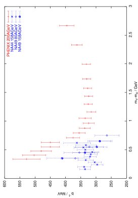
Figure 4: Fit parameters for the feed-down corrected antiproton spectra

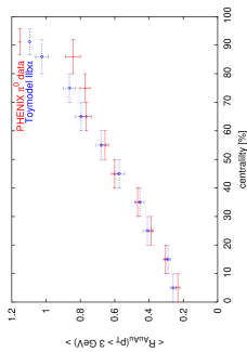
Figure 4: Results for the Toymodel II b $\alpha$ with $\Delta E\propto N_{g}^{2}E$ and inhomogeneous energy density distribution

Gluons carry colour octet charges which means that they cannot serve as endpoint for a triplet string. But they can be situated in the middle of a string with the colour connected to the anticolour-end and the anticolour with the colour-end of the string. If a quark for example radiates gluons in a parton shower à la DGLAP the gluons will be aligned in the same string as the quark (Fig. 4).

2 Independent Fragmentation

In the framework of independent fragmentation it is assumed that each parton hadronises on its own, i.e. the fragmentation of a jet system is an incoherent sum of the fragmentations of each parton. The procedure has to be carried out in the overall c.m. system.

There is an iterative approach somewhat similar to the Lund model: A jet arising from the fragmentation of a quark is split into a meson and a remainder jet with lower energy and momentum. The sharing of energy-momentum is governed by a fragmentation function, actually the same functions can be used for string and independent fragmentation. Flavour and transverse momentum are conserved in each break-up. It is assumed that the formation of a meson does not depend on the energy of the remainder jet so that the step can be iterated resulting in a sequence of hadrons. There is, however, one problem with very small values of $z$: They lead to backward moving hadrons (i.e. $p_{\parallel}<0$) that have to be rejected.

Although flavour and transverse momentum are conserved locally this is not the case in the global balance. In the end there will always be an unpaired (anti)quark left behind. There may also be hadrons with $p_{\parallel}<0$, that were removed their energy and momentum being lost for the jet. Thus overall energy, momentum, charge and flavour are not conserved. This also applies to jet systems since each parton hadronises separately.

There are several possibilities for the treatment of gluon jets. Since a gluon is expected to result in a softer jet it is sensible to split the gluon perturbatively in a $q\bar{q}$ pair, then the same fragmentation function as for the quark jets can be used.

Apart from the non-conservation of energy-momentum and flavour there are two more conceptual weaknesses: the issues of Lorentz invariance and collinear divergences. The result of independent fragmentation depends on the coordinate frame and is thus not Lorentz invariant. This problem is circumvented by requiring the fragmentation to take place in the overall c.m. frame. The colliniear divergence, on the other hand, leads to problems in connection with parton showers. A system of collinear partons leads to a much higher hadron multiplicity than a single parton with the same energy.

Chapter 2 Hunting the Quark Gluon Plasma

1 QCD Predictions

At high temperatures and densities the long range interactions between quarks are dynamically screened (similar to Debye screening). Only the very short range interactions remain but here the coupling is weak so that the quarks and gluons are quasi-free and thus deconfined. Furthermore chiral symmetry is restored at apparantly the same critical temperature $T_{c}$. This phase of deconfined quarks and gluons and restored chiral symmetry is called the quark-gluon plasma (QGP) [7]. This is not unexpected since spontaneously broken symmetries (such as chiral symmetry) are often restored at high temperatures through a phase transition [8]. An important question is now whether there is a phase transition from hadronic to deconfined matter. Recent results of simulations of QCD on the lattice indicate a phase transition at a critical temperature $T_{c}\simeq 170\,\mathrm{MeV}$ which corresponds to an energy density of $\epsilon_{c}\simeq 1\,\mathrm{GeV\,fm^{-3}}$ [9]. This is too low for pertubation theory to be applicable and one has to rely on lattice QCD. Although great progress has been made in this field there are still major problems. It has, for instance, so far not been possible to determine the order of the phase transition and many calculations are done for vanishing baryon chemical potential (i.e. vanishing baryon number) which is a good approximation for the early universe and the LHC but not for AGS, SPS and RHIC [7, 8].

2 Models

There is a large variety of different models for heavy-ion collisions that are based on largely different ideas and assumptions. Only a short overview over the main classes can be given here [7, 8].

Statistical models

(e.g. [10]) assume that local thermal and chemical equilibrium is achieved during the collision. The starting point is a hadron gas that can either be created directly in the collision or the product of the hadronisation of a QGP. It is described as an ideal hadron gas using a canonical or grand canonical formalism. The gas expands until inelastic interactions cease, then the composition of the system is fixed (chemical freeze-out). At some point the mean free path becomes so long that also the elastic interactions stop (thermal freeze-out). When resonance decays are included statistical models can yield the relative abundancies of hadron species as they are measured by experiments.
Comparison of the model results with data can help to clarify if, or to what extent, equilibrium is achieved. The freeze-out temperature and (hadron) chemical potential can be determined by fitting the model to data.

Parton Cascades

(e.g. [11]) are detailed microscopic models that describe the collision of two nuclei in a perturbative QCD framework. The first step is the decomposition of the nuclei in partons according to measured structure functions. The interactions during the collisions are treated as perturbative scatterings with initial and final state radiation. The last stage is the hadronisation of the partons using the Lund string model.
Parton cascades predict a rapid thermalisation (proper time scale 0.3-0.5 fm) and a chemical equilibration that takes somewhat longer (several fm). The plasma is initially gluon rich due to the larger cross sections for gluons.

Hadronic Transport models

(e.g. [12]) are formulated in a hadron basis although some also include non-hadronic elements such as quarks and strings. The heavy-ion collision is described as a sequence of collisions of constituents (mesons, baryons, quarks,…). Partonic degrees of freedom are not treated explicitly so that no phase transition can occur.
Hadronic models provide a very useful background for other models because it is important to understand which phenomena can be described in terms of hadronic physics.

Hydrodynamic models

(e.g. [13, 14]) are macroscopic kinetic models that are based on the assumption of local equilibrium and energy-momentum conservation. The nuclei are described as fluids and in some models a third fluid can be created in the collisions. Starting from the colliding nuclei, an equilibrated QGP or hadronic matter the time evolution of the system can be studied until hadronic freeze-out.
These are the only dynamical models in which a phase transition can be incorporated explicitly via the equations of state.

3 Observables

The number of observables that have been suggested as signatures of QGP formation is so large that it is impossible to discuss all of them here. Instead three of the most popular will be presented without going into details.

Strangeness Enhancement

The production of strange hadrons is suppressed in pp collisions and the suppression increases with the strangeness content of the respective hadron. This has been argued to be due to the higher strange quark mass [7, 8]. In a QGP strangeness saturation via $s\bar{s}$ pair production is expected which would significantly increase the yields of strange particles [8]. The estimated time scale of several fm for strangeness equilibration is maybe too long for a complete saturation, but an increased strangeness content leads to increased strange particle yields in any case. If it is the statistical hadronisation of a strangeness-enhanced deconfined phase that is observed a stronger enhancement of multistrange hadrons is expected. The enhancement factor for a hadron containing $N$ strange quarks is $E_{s}^{N}$ where $E_{s}$ is the global enhancement factor. Hadron rescattering scenarios lead to the opposite behaviour [15].

A QGP formed at AGS or SPS would have nonzero chemical potentials for $u$ and $d$ leading to an ordering in the quark abundances: The densities of $u$ and $d$ is higher than that of $s$ and $\bar{s}$, which is higher than the $\bar{u}$ and $\bar{d}$ density. This means that at freeze-out the combination of a $\bar{s}$ with a $u$ or $d$ to $K^{+}$ or $K^{0}$ is more likely than the $s\bar{u}$ and $s\bar{d}$ combination ($K^{-}$ and $\bar{K}^{0}$). Thus the $K^{+}/\pi^{+}$ ratio should be different from $K^{-}/\pi^{-}$ in case of QGP formation. Unfortunately, the argumentation has several drawbacks. One is that the strange particle abundancies after freeze-out of a QGP are very close to those in an equilibrated hadron gas with the same entropy content [7] so that it is difficult to unambiguously relate different ratios to QGP formation.

Chemical Equilibrium and Freeze-Out

If the observed hadrons are produced in the hadronisation of an equilibrated QGP they should inherit the property of chemical equilibrium. This also includes the disappearance of the strangeness suppression. From a statistical model fit to data the freeze-out temperature and chemical potential can be found. These values can then be compared to lattice QCD calculations for the phase boundary. A chemical freeze-out close to or at the phase boundary suggests that the hadrons originate from a deconfined medium and that the chemical composition is established during the phase transition.

Charmonium Suppression

In a QGP colour screening reduces the range of the attractive force between quarks and antiquarks and thereby prevents $c\bar{c}$ pairs from binding. It is therefore expected that the more loosely bound $\psi^{\prime}$ and $\chi_{c}$ states start to be suppressed at a lower temperature than $J/\psi$ [15]. There is evidence from lattice calculations that the $1S$ states $J/\psi$ and $\eta_{c}$ survive up to $1.5\,T_{c}$ whereas the $\chi_{c}$ states are dissolved already at $1.1\,T_{c}$ [16].

$c\bar{c}$ pairs are produced as small configurations and the evolution to the larger charmonium state takes approximately 1 fm. Thus the $J/\psi$ should survive if it escapes fast enough, i.e. if it has a high transverse momentum or if the QGP expands very rapidly [8].

There is, however, a problem with charmonium suppression as a clear signal of a QGP and that is the charmonium suppression observed in pA collisions. Interactions with comoving particles can break the charmonium apart, the broadened intrinsic transverse momentum distribution (Cronin effect) and the absorption on nucleons also contribute to the suppression. The hard contribution to the charmonium-nucleon cross section can be calculated using perturbative QCD and is in good agreement with pA data when the formation length and feeding of the $J/\psi$ from $\psi^{\prime}$ and $\chi_{c}$ are taken into account [17, 18]. A QGP would thus manifest itself in an anomalously high charmonium suppression.

Hadronic cascade models attempt to explain the charmonium suppression in AA collisions by interactions with comoving hadrons. They also predict a stronger suppression of $\psi^{\prime}$ than of $J/\psi$ [8].

The statistical hadronisation model [19] assumes that all charm quarks are produced in hard interactions in the early stage of the collision and are then equilibrated in a QGP (thermal but not chemical equilibrium). The charmed hadrons are formed at freeze-out according to statistical laws.

A similar behaviour is expected for the bottonium states.

Finding signatures that can unambiguously be related to the presence of a QGP is very difficult and it is often possible to describe the effects, that where believed to be a clear signal, with hadronic scenarios. It is thus likely that the proof for QGP formation will be based on several effects, each of which alone cannot provide a convincing proof.

The search at AGS and SPS was based on soft physics such as the strangeness enhancement. They are mostly sensitive to the latest stage of the collision after hadronisation. At RHIC also hard probes like jet quenching become accessible, which provide information on the very early phase of the collision since hard scatterings occur even before the equilibration of the QGP.

Chapter 3 Jet Quenching

When a hard (i.e. large momentum transfer) scattering takes place in the interaction of two protons the two scattered partons leave the protons with high transverse momentum. In the centre-of-momentum frame they are emitted back-to-back in azimuthal angle due to momentum conservation. The fragmentation of each of these energetic partons gives rise to a jet, i.e. a spray of hadrons with small angles relative to the momentum of the parton. The energy distribution inside the jet is determined by the fragmentation function (Sec. 1). The typical jet signature is a large energy deposition localised in a small solid angle. In two-jet events the two jets are opposite in azimuth and have nearly the same energy (small deviations arise from differences in the momentum fraction $x$ carried by the partons). Partons with $p_{\perp}\gtrsim 3-4\,\mathrm{GeV}$ are expected to give rise to jets.

In a soft interaction the cross section for producing a given total transverse momentum rises only slowly with the collision energy $\sqrt{s}$ since the particle multiplicity rises logarithmically with $s$ and the mean $p_{\perp}$ also depends only little on $s$. In hard interactions on the other hand the cross section for producing a given total transverse momentum rises rapidly with $s$ because the required $x\sim\sum|p_{\perp}|/\sqrt{s}$ gets smaller and the parton distribution functions rise rapidly towards smaller $x$. Therefore the hard parton-parton scattering dominates the cross section for sufficiently high $\sum|p_{\perp}|$ and $s$ [20].

fmf1pic (84,53) em,ep fermionem,Zee,ep gluonZee,Zff fermionfb,Zff,f fb,f

fmf2pic (84,53) em,ep fermionem,Zee,ep gluonZee,Zff fermionf,Zff,fb fb,f

fmf3pic (84,53) em,ep gluonem,Zee,ep gluonZee,Zff fermionf,Zff,fb fb,f

fmf4pic (84,53) em,ep gluonem,Zee,ep gluonZee,Zff gluonf,Zff,fb fb,f

fmf5pic (84,53) em,ep fermionfb,Zee,em gluonZee,Zff fermionep,Zff,f fb,f

fmf6pic (84,53) em,ep gluonem,Zee gluonZff,ep fermionfb,Zee,Zff,f fb,f

fmf7pic (84,53) em,ep fermion,tension=2fb,Zee,Zff,f gluonep,Zee gluonZff,em fb,f (.6w,.25h)Zee (.6w,.75h)Zff

fmf8pic (84,53) em,ep gluonem,Zee gluonZff,ep gluonfb,Zee,Zff,f fb,f

Figure 1: Examples for Feynman diagrams for parton-parton scattering to lowest order

The lowest order parton-parton scattering ($a+b\to c+d$) cross section is of the form [20]

$$\frac{\mathrm{d}\hat{\sigma}}{\mathrm{d}\hat{t}}(ab\to cd)=\frac{1}{16\pi^{2}\hat{s}^{2}}|\mathcal{M}|^{2}$$ (1)

The quantities with hats refer to the parton level and $|\mathcal{M}|^{2}$ is the matrix element squared. Spins and colours are averaged in the initial and summed in the final state. $\hat{s}$, $\hat{t}$, $\hat{u}$ are the Mandelstam variables

$$\hat{s}\!\!\! = \!\!\!(p_{a}+p_{b})^{2}=(p_{c}+p_{d})^{2}$$ (2)

$$\hat{t}\!\!\! = \!\!\!(p_{a}-p_{c})^{2}=(p_{b}-p_{d})^{2}$$ (3)

$$\hat{u}\!\!\! = \!\!\!(p_{a}-p_{d})^{2}=(p_{b}-p_{c})^{2}$$ (4)

Figure 1 shows a few examples of processes that contribute to lowest order to the parton-parton scattering.

With the help of the relation

$$p_{\perp}^{2}=\frac{\hat{u}\hat{t}}{\hat{s}}=\frac{\hat{s}}{4}\sin^{2}\hat{\theta}$$ (5)

and neglecting the intrinsic transverse momentum of the partons the cross section can be written as

$$\frac{\mathrm{d}\hat{\sigma}}{\mathrm{d}(p_{\perp}^{2})}=\frac{1}{\cos\hat{\theta}}\frac{\mathrm{d}\hat{\sigma}}{\mathrm{d}\hat{t}}=\frac{\hat{s}}{\hat{t}-\hat{u}}\frac{\mathrm{d}\hat{\sigma}}{\mathrm{d}\hat{t}}$$ (6)

Then the lowest order QCD cross section for two-jet production in a collision of two hadrons $A$ and $B$ is given by [20]

$$\!\!\!\!\!\!\!\!\frac{\mathrm{d}\sigma}{\mathrm{d}(p_{\perp}^{2})}(AB\to 2\ \mathrm{jets})$$ (7)

$$\!\!\!=\sum_{abcd}\int\limits_{0}^{1}\!\mathrm{d}x_{a}\!\int\limits_{0}^{1}\!\mathrm{d}x_{b}\,\Theta\left(x_{a}x_{b}-\frac{4p_{\perp}^{2}}{s}\right)f_{a/A}(x_{a},Q^{2})f_{b/B}(x_{b},Q^{2})\frac{\mathrm{d}\hat{\sigma}}{\mathrm{d}(p_{\perp}^{2})}(ab\to cd)$$

There are many ways to express the differential cross section, a very useful relation is

$$E\frac{\mathrm{d}^{3}\sigma}{\mathrm{d}^{3}p}=\frac{\mathrm{d}^{3}\sigma}{p_{\perp}\mathrm{d}\phi\,\mathrm{d}y\,\mathrm{d}p_{\perp}}=2\frac{\mathrm{d}^{3}\sigma}{\mathrm{d}\phi\,\mathrm{d}y\,\mathrm{d}(p_{\perp}^{2})}$$ (8)

The agreement between the parton model calculations and data is impressive, a few examples are shown in Figure 2.

Insofar as Bjorken scaling holds in deep inelastic scattering this means that the dependence on any dimensionful parameter has disappeared. A similar property in hadron-hadron collisions leads to factorised cross sections such that single-particle inclusive cross sections are for high $p_{\perp}$ of the form

$$E\frac{\mathrm{d}^{3}\sigma}{\mathrm{d}^{3}p}\longrightarrow p_{\perp}^{-n}F(x_{\perp},\theta)\qquad x_{\perp}=\frac{2p_{\perp}}{\sqrt{s}}$$ (9)

where $\theta$ is the centre-of-mass production angle [21]. This factorisation in a power of $p_{\perp}$ and a dimensionless function $F$ is called power law scaling.

The hadron-hadron cross sections are well described by a parametrisation of the form [22]

$$E\frac{\mathrm{d}^{3}\sigma}{\mathrm{d}^{3}p}=C\left(\frac{p_{0}}{p_{\perp}+p_{0}}\right)^{n}$$ (10)

where $C$, $p_{0}$ and $n$ are free parameters. Although it yields a very good description of the shape of the cross sections this parametrisation is not suited for extrapolations since it doesn’t include the dependence on energy and rapidity.

Figure 2: Left: Comparison of pQCD calculations for spectra of charged hadrons to data, solid lines are calculations with intrinsic $k_{\perp}$, dash-dotted lines are without [23]. Right: Invariant cross section for neutral pion production, lines are QCD calculations with different parameters [24].

The hard part of the $p_{\perp}$-spectra in pp collisions is well understood in terms of pQCD. Collisions of nuclei are more complicated, nevertheless, because of the hard scale involved, high-$p_{\perp}$ hadrons are especially suited to investigate nuclear modifications. The perturbative processes happen on very short distance and time scales so that it is likely that the hard scattering in nucleus-nucleus collisions will look exactly like in proton-proton because it doesn’t feel the surrounding. However, the pdf’s might be different from the ordinary nucleon pdf’s.

In the following considerations it is assumed that a quark-gluon plasma is formed in central nucleus-nucleus collisions. Hard scatterings can thus take place anywhere in the overlap region of the colliding nuclei, i.e. inside the plasma. Consequently the scattered partons have to traverse it. Since the quark-gluon plasma is a phase with very high colour charge density the partons should interact strongly with it. The parton, that has a much higher energy than its environment, is expected to lose a considerable fraction of it in the plasma. In the subsequent hadronisation this leads to a softer jet with lower mean momentum and number of hadrons. This expected suppression of high-$p_{\perp}$ hadrons as compared to scaled pp yields is commonly referred to as jet quenching.

The amount of energy loss depends on the length of the parton’s path trough the plasma and is thus given by the geometry of that particular event (i.e. centrality of the collision, position of the hard interaction in the plasma, scattering angle of the partons). If the energy loss in the plasma is large it should be possible that a parton with a long path loses essentially all its energy and does not produce a jet. This jet-disappearance would be a clear signal for the QGP, but it is very difficult to measure the non-existence of a jet experimentally. A possible way out is offered by two-jet correlations. In fact, if the hard scattering took place off the centre of the plasma and one parton has a shorter way out so that it loses less energy. Consequently the other one has to travel a longer distance through the plasma and may get thermalised (i.e. lose essentially all its energy). The parton with the shorter path length in the plasma may still have enough energy to produce a jet containing high-$p_{\perp}$ hadrons. This can then be seen as an event with only one clear jet that can be identified experimentally.

The observation of jet quenching, i.e. suppression of high-$p_{\perp}$ hadrons and disappearance of two-jet events would be a signal for the formation of a QGP. This search is currently going on at RHIC (Ch. 2).

A currently accepted scenario for the energy loss mechanism is induced gluon radiation. One possible approach to this problem is to consider the scattering off static scattering centres [25]. In the approximation that successive scatterings are independent and the incident parton has very high energy the radiation spectrum induced by multiple scattering can be derived (Sec. 6).

Nevertheless, this may not be the only explanation. It is the aim of this study to investigate if soft gluon exchanges can also contribute significantly to the jet quenching. A model for this will be dicussed in detail in Chapter 9. Furthermore the general properties of partonic energy loss will be studied in Chapter 10. The main focus will be on the question if the experimental data clearly exhibit signs that enable to discriminate between a bremsstrahlung and a scattering dominated parton energy loss in the plasma phase.

It is in fact probable that both effects – scattering and radiation – contribute to the overall jet quenching. The parton scatters off a QGP constituent and is deflected (and loses energy) which induces gluon bremsstrahlung (and thereby additional energy loss). There might also be quantum mechanical interference between the two processes. In the gluon bremsstrahlung models the effect of the scattering is neglected. The model studied here concentrates in a complementary fashion on the scattering and does not take into account gluon radiation. When both effects have been studied separately it will hopefully be possible to combine the two into a more complete model.

Chapter 4 Basics of Heavy Ion Physics

Collisions of relativistic heavy nuclei are very complex processes with many interesting effects that are not well understood today. This chapter cannot cover all of these exciting phenomena, instead only the effects that are relevant for this study will be presented briefly.

1 Glauber models

In Glauber models it is assumed that the interactions of two nuclei can be viewed as an incoherent superposition of nucleon-nucleon interactions. A collision of two nuclei is then characterised by the mean number of binary nucleon-nucleon collisions $\langle N_{\mathrm{coll}}\rangle$ and the mean number of participating nucleons $\langle N_{\mathrm{part}}\rangle$. Both numbers depend on the impact parameter $b$. Participating nucleons are those that encountered at least one binary collision.

There exist many variations on the theme, the model introduced in [26] will be dicussed briefly as a representative.

The nuclei $A$ and $B$ are characterised by the spherical nuclear density $n_{A,B}(r)$ satisfying

$$\int\!\mathrm{d}^{3}r\,n_{A}(r)=A$$ (1)

The nuclear density is described rather well by a Woods-Saxon distribution

$$n_{A}^{\mathrm{WS}}(r)=\frac{n_{0}}{e^{(r-R_{A})/d}+1}\quad\mathrm{with}\quad n_{0}=\frac{3A}{4\pi R_{A}^{3}(1+\pi^{2}d^{2}/R_{A}^{2})}$$ (2)

A simpler alternative that unfortunately doesn’t yield as good results is the sharp sphere

$$n_{A}^{ss}(r)=\frac{3A}{4\pi R_{A}^{2}}\Theta(R_{A}^{2}-r^{2})$$ (3)

The $z$-direction is chosen to be the beam axis and the impact parameter $\vec{b}$ lies in the plane perpendicular to $z$ and points from beam to target. The thickness function $T_{A}(b)$ is given by

$$T_{A}(b)=\int\limits_{-\infty}^{\infty}\!\mathrm{d}z\,n_{A}(\sqrt{b^{2}+z^{2}})$$ (4)

with

$$\int\!\mathrm{d}^{2}b\,T_{A}(b)=A$$ (5)

$T_{A}$ can be interpreted as the part of the nucleus $A$ ”seen” by a nucleon passing through it with impact parameter $b$. For central collisions (i.e. small values of $b$) $T_{A}$ is proportional to $A^{1/3}$. When going to nucleus-nucleus collisions the product of the two thickness functions has to be integrated in the overlap region in order to get the nuclear overlap $T_{AB}(b)$:

$$T_{AB}(b)=\int\!\mathrm{d}^{2}b_{1}\,\mathrm{d}^{2}b_{2}\,\delta^{2}(\vec{b}-\vec{b}_{1}-\vec{b}_{2})T_{A}(b_{1})T_{B}(b_{2})\,$$ (6)

with

$$\int\!\mathrm{d}^{2}b\,T_{AB}(b)=AB$$ (7)

The product $\sigma^{\mathrm{NN}}_{\mathrm{inel}}T_{AB}(b)$, where $\sigma^{\mathrm{NN}}_{\mathrm{inel}}$ is the total inelastic nucleon-nucleon cross section at the respective collision energy, can be interpreted as the mean number of binary collisions $\langle N_{\mathrm{coll}}\rangle$ at impact parameter $b$. The total nucleus-nucleus cross section is obtained by integrating $\sigma^{\mathrm{NN}}_{\mathrm{inel}}T_{AB}(b)$ over $b$:

$$\sigma^{AB}_{\mathrm{inel}}=\int\!\mathrm{d}^{2}b\,\sigma^{\mathrm{NN}}_{\mathrm{inel}}T_{AB}(b)=AB\sigma^{\mathrm{NN}}_{\mathrm{inel}}$$ (8)

Similarly $T_{AB}(b)$ can be multiplied with any cross section to get the mean number of events of a particular kind per $AB$ collision at impact parameter $b$.

The mean number of participants is given by

$$\langle N_{\mathrm{part}}(b)\rangle=\int\!\mathrm{d}^{2}b_{1}\,\mathrm{d}^{2}b_{2}\,\delta(\vec{b}-\vec{b}_{1}-\vec{b}_{2})\left\{T_{A}(b_{1})p_{\geq 1}^{(B)}(b_{2})+T_{B}(b_{2})p_{\geq 1}^{(A)}(b_{1})\right\}\,$$ (9)

where $p_{\geq 1}^{(A)}(b_{1})$ is the probability for a nucleon passing through the nucleus $A$ with impact parameter $b_{1}$ to take part in at least one interaction. It can be obtained from the Binomial distribution:

$$p_{\geq 1}^{(A)}(b_{1}) = 1-{A\choose 0}\left(\frac{\sigma^{\mathrm{NN}}_{\mathrm{inel}}T_{A}(b_{1})}{A}\right)^{0}\left(1-\frac{\sigma^{\mathrm{NN}}_{\mathrm{inel}}T_{A}(b_{1})}{A}\right)^{A-0}$$ (10)

$$= 1-\left(1-\frac{\sigma^{\mathrm{NN}}_{\mathrm{inel}}T_{A}(b_{1})}{A}\right)^{A}$$

$$\approx 1-e^{-\sigma^{\mathrm{NN}}_{\mathrm{inel}}T_{A}(b_{1})}\qquad\mathrm{for\ large\ }A$$ (11)

For the most central and symmetric (i.e. $A=B$) collisions $\langle N_{\mathrm{part}}\rangle$ is linear in $A$ whereas $\langle N_{\mathrm{coll}}\rangle$ is proportional to $A^{4/3}$. It turns out that soft particle production in heavy ion collisions scales with the number of participants while hard processes scale with the number of binary collisions.

2 Quantum Statistics of an Ideal Quark-Gluon Gas

As a consequence of the energy dependence of the strong coupling constant $\alpha_{s}$ the interactions among quarks and gluons become weak at high energy densities. Thus a gas of non-interacting ultra-relativistic quarks and gluons can be used as an approximation.

The particle numbers are not fixed so that the grand canonical formalism has to be used (see e.g. [27]). Let $\vec{\nu}$ be a set of quantum numbers characterising a one-particle state, $n(\vec{\nu})$ the occupation number of that state and $E(\vec{\nu})$ the corresponding one-particle energy. $\{n(\vec{\nu})\}$ is the complete set of occupation numbers. Then the grand canonical partition function for bosons is

$$\Xi^{(B)}(T,V,\mu) = \sum_{\mathrm{all\ states}}\exp(-\beta(E_{\mathrm{tot}}-\mu N))$$ (12)

$$= \sum_{\{n(\vec{\nu})\}}\exp\left(-\beta\sum_{\vec{\nu}}n(\vec{\nu})(E(\vec{\nu})-\mu)\right)$$

$$= \sum_{\{n(\vec{\nu})\}}\prod_{\vec{\nu}}\{\exp(-\beta(E(\vec{\nu})-\mu))\}^{n(\vec{\nu})}$$

$$= \prod_{\vec{\nu}}\sum_{n(\vec{\nu})=0}^{\infty}\{\exp(-\beta(E(\vec{\nu})-\mu))\}^{n(\vec{\nu})}$$

$$= \prod_{\vec{\nu}}\frac{1}{1-\exp(-\beta(E(\vec{\nu})-\mu))}$$

where $\beta=1/T$, $\mu$ is the chemical potential and $E_{\mathrm{tot}}$ and $N$ denote the total energy and number of particles in the ensemble. The partition function for fermions can be derived in a similar fashion.

$$\Xi^{(F)}(T,V,\mu) = \prod_{\vec{\nu}}\sum_{n(\vec{\nu})=0}^{1}\{\exp(-\beta(E(\vec{\nu})-\mu))\}^{n(\vec{\nu})}$$ (13)

$$= \prod_{\vec{\nu}}\frac{1}{1+\exp(-\beta(E(\vec{\nu})-\mu))}$$

$$\Rightarrow\ln\Xi(T,V,\mu)=\pm\sum_{\vec{\nu}}\ln\left(1\pm e^{-\beta(E(\vec{\nu})-\mu)}\right)$$ (14)

where the plus sign applies to fermions and the minus sign to bosons. If the energy levels are not discrete but continuous the sum can be transformed into an integral yielding

$$\ln\Xi(T,V,\mu)=\pm\int\!\frac{\mathrm{d}^{3}q\,\mathrm{d}^{3}p}{(2\pi)^{3}}\,\ln\left(1\pm e^{-\beta(E(\vec{\nu})-\mu)}\right)$$ (15)

where $p$ and $q$ are momentum and spacial coordinates.

The mean occupation number of a state is given by

$$\bar{n}(\vec{\nu})=-\frac{\partial\ln\Xi}{\partial(\beta E(\vec{\nu}))}=\frac{1}{e^{-\beta(E(\vec{\nu})-\mu)}\pm 1}$$ (16)

For the quark gluon gas it is helpful to assume that the QGP is net baryon-free as will be the case in ultra-relativistic ion-ion collisions. Then the gluon as well as the quark chemical potential vanishes and the numbers of quarks and antiquarks are equal. Furthermore, it has to be taken into account that the energy levels are degenerate so that the mean occupation number is

$$\bar{n}_{p}=\frac{g}{e^{E/T}\pm 1}\quad\mathrm{with}\quad E=\sqrt{\vec{p}\,^{2}+m^{2}}$$ (17)

where again the plus (minus) sign applies to fermions (bosons) and $g$ is the degeneracy. It is given by the number of flavours times the number of colours times the number of polarisations:

$$g_{g}=2(\mathrm{polarisation})\cdot 8(\mathrm{colour})=16$$ (18)

$$g_{q}=g_{\bar{q}}=N_{f}(\mathrm{flavour})\cdot 2(\mathrm{polarisation})\cdot 3(\mathrm{colour})=6N_{f}$$ (19)

If the masses are neglected the particle and energy densities can easily be calculated:

$$n_{g}\!\!\! = \!\!\!\frac{1}{V}\frac{1}{(2\pi)^{3}}\int\!\mathrm{d}^{3}q\,\mathrm{d}^{3}p\,\bar{n}_{p}=\frac{4\pi g_{g}}{(2\pi)^{3}}\int\limits_{0}^{\infty}\!\mathrm{d}p\,\frac{p^{2}}{e^{p/T}-1}$$ (20)

$$= \!\!\!\frac{g_{g}}{2\pi^{2}}T^{3}\int\limits_{0}^{\infty}\!\mathrm{d}\xi\,\frac{\xi^{2}}{e^{\xi}-1}=\frac{g_{g}}{2\pi^{2}}T^{3}2\,\zeta(3)\simeq 1.2\,\frac{g_{g}}{\pi^{2}}T^{3}$$

$$n_{q}\!\!\! = \!\!\!n_{\bar{q}}=\frac{1}{V}\frac{1}{(2\pi)^{3}}\int\!\mathrm{d}^{3}q\,\mathrm{d}^{3}p\,\bar{n}_{p}\ =\frac{4\pi g_{q}}{(2\pi)^{3}}\int\limits_{0}^{\infty}\!\mathrm{d}p\,\frac{p^{2}}{e^{p/T}+1}$$ (21)

$$= \!\!\!\frac{g_{q}}{\pi^{2}}\,T^{3}d(3)\simeq 0.9\,\frac{g_{q}}{\pi^{2}}T^{3}$$

$$\epsilon_{g}\!\!\! = \!\!\!\frac{1}{V}\frac{1}{(2\pi)^{3}}\int\!\mathrm{d}^{3}q\,\mathrm{d}^{3}p\,p\,\bar{n}_{p}\ =\frac{3g_{g}}{\pi^{2}}\,T^{4}\,\zeta(4)=\frac{\pi^{2}g_{g}}{30}\,T^{4}$$ (22)

$$\epsilon_{q}\!\!\! = \!\!\!\epsilon_{\bar{q}}=\frac{3g_{q}}{\pi^{2}}\,T^{4}\,d(4)=\frac{7\pi^{2}g_{q}}{240}\,T^{4}$$ (23)

with

$$\zeta(\xi)=\frac{1}{\Gamma(\xi)}\int\limits_{0}^{\infty}\!\mathrm{d}\alpha\,\frac{\alpha^{\xi-1}}{e^{\alpha}-1}\qquad\mathrm{and}\qquad d(\xi)=\frac{1}{\Gamma(\xi)}\int\limits_{0}^{\infty}\!\mathrm{d}\alpha\,\frac{\alpha^{\xi-1}}{e^{\alpha}+1}$$ (24)

Thus the energy per particle is given by

$$\frac{\epsilon_{g}}{n_{g}}=3T\,\frac{\zeta(4)}{\zeta(3)}\simeq 2.7\,T$$ (25)

$$\frac{\epsilon_{q}}{n_{q}}=3T\,\frac{d(4)}{d(3)}\simeq 3.2\,T$$ (26)

and the total pressure can be obtained from the equation of state:

$$p_{qg}=\frac{1}{3}\,\epsilon_{qg}=\frac{1}{3}(\epsilon_{g}+\epsilon_{q}+\epsilon_{\bar{q}})=\frac{\pi^{2}}{90}\left(16+\frac{21}{2}N_{f}\right)T^{4}$$ (27)

3 The Bjorken Model

The Bjorken model [13] is applicable to energetic ion-ion collisions with $\sqrt{s}\geq 100\,\mathrm{A\,GeV}$. It is based on the assumption that the inclusive particle multiplicity as a function of rapidity shows a ”central plateau”, i.e. particle production looks the same in all centre-of-mass-like frames. The second assumption is that the nuclei are essentially transparent to each other. The net baryon number is thus contained in the receding remnants of the nuclei and the central rapidity region is net baryon-free (i.e. the baryon chemical potential vanishes).

After the collision the two Lorentz contracted nuclei recede from the collision point with nearly speed of light. Between them is a dense and hot system that expands longitudinally. The expansion velocity is $z/t$ where $z=0$ and $t=0$ refer to the collision point and time. From the charged particle multiplicity observed in nucleon-nucleus collisions the initial energy density is estimated:

$$\epsilon_{0}=\epsilon(\tau_{0})\approx 1-10\,\mathrm{\frac{GeV}{fm^{3}}}$$ (28)

for an initial proper time

$$\tau_{0}=1\,\mathrm{fm/c}\qquad\tau=\sqrt{t^{2}-z^{2}}$$ (29)

This relatively high number suggests that the system rapidly comes into local thermal equilibrium and afterwards follows a hydrodynamic evolution. It is thus possible to define a local energy density $\epsilon(\tau,y)$, pressure $p(\tau,y)$, temperature $T(\tau,y)$ and four-velocity $u_{\mu}(\tau,y)$.

The first assumption implies that the initial condition possesses a symmetry under Lorentz transformations which is preserved during the subsequent evolution. This means that the energy density, pressure etc. cannot depend on the rapidity.

Figure 1: Space-time diagram of longitudinal evolution of the quark-gluon plasma [13]

Neglecting the viscosity and heat conduction the energy-momentum tensor becomes

$$T_{\mu\nu}=(\epsilon+p)u_{\mu}u_{\nu}-g_{\mu\nu}p$$ (30)

It is conserved, i.e.

$$\frac{\partial T_{\mu\nu}}{\partial x_{\mu}}=0\ .$$ (31)

Making use of the fact that the occuring quantities depend only on the proper time this expression simplifies to

$$\frac{\mathrm{d}\epsilon}{\mathrm{d}\tau}=-\frac{\epsilon+p}{\tau}$$ (32)

This can also be written as

$$\frac{\mathrm{d}\epsilon}{\mathrm{d}\tau}=\frac{\mathrm{d}\epsilon}{\mathrm{d}p}\frac{\mathrm{d}p}{\mathrm{d}T}\frac{\mathrm{d}T}{\mathrm{d}\tau}=-\frac{\epsilon+p}{\tau}=-\frac{Ts}{\tau}$$ (33)

where $s$ is the entropy density. With the help of

$$\frac{\mathrm{d}p}{\mathrm{d}T}=\frac{S}{V}=s\quad\mathrm{and}\quad\frac{\mathrm{d}\epsilon}{\mathrm{d}p}=\frac{1}{v_{s}^{2}}$$ (34)

($v_{s}$ is the velocity of sound) the differential equation for the time dependence of the temperature is obtained:

$$\frac{1}{T}\frac{\mathrm{d}T}{\mathrm{d}\tau}=-\frac{v_{s}^{2}}{\tau}$$ (35)

In the case of an ideal ultra-relativistic gas the equation of state is $\epsilon=3p$. Inserting this into Equations 32, 34 and 35 leads to the result that the time dependence of the energy density and temperature is given by

$$\epsilon(\tau)\propto\tau^{-4/3}$$ (36)

and

$$T(\tau)\propto\tau^{-1/3}$$ (37)

respectively.

The simple picture of purely longitudinal expansion has to be modified when the distance between the nuclei becomes comparable to their diameter. There is a rarefaction front moving inward from the periphery at the velocity of sound. Under the assumption of a time independent velocity of sound the equation for the rarefaction front is

$$\rho(t)=R-\int\limits_{0}^{\sqrt{t^{2}-z^{2}}}\!\mathrm{d}t^{\prime}\,v_{s}=R-v_{s}\sqrt{t^{2}-z^{2}}$$ (38)

At transverse distances smaller than the rarefaction front the system continues to expand longitudinally because the information that there is a boundary has not yet reached this region. Outside the front the gas expands radially outward and cooles faster than during longitudinal expansion.

Figure 2: Geometry of fluid expansion near the edge of the nuclei [13]

4 Azimuthal Anisotropy

..................................................................................................................................................................................................................................................................................................................................................................................................................................................................................................................................................................................................................................................................................................................................................................................................................................................................................................................................................................................................................................................................................................................................................................................................................................................................................................................................................................................................................   .......  ......................................$y$...........................................................................................................................................................................................................................................................................  ............................................................................................................................................................................................................................................................................$b$$x$$\phi$          

Figure 3: Overlap region in a non-central collision

The beam axis ($z$ axis) and the impact parameter $b$ define the reaction plane. In non-central collisions the overlap region has an almond like shape (Fig. 3) so that the pressure gradient depends on the direction. This leads to an asymmetric particle emission that can be described by

$$E\frac{\mathrm{d}^{3}N}{\mathrm{d}^{3}p}=\frac{1}{2\pi}\frac{\mathrm{d}^{2}N}{p_{\perp}\mathrm{d}p_{\perp}\mathrm{d}y}\left[1+\sum_{n=1}^{\infty}2v_{n}\cos(n\phi)\right]$$ (39)

where $\phi$ is the azimuthal angle with respect to the reaction plane [9].

An important feature is that the odd Fourier coefficients change sign at mid-rapidity whereas the even are symmetric. It is common to discuss collective flow in terms of the lowest order coefficients in the Fourier expansion in Equation 39. They can be determined experimentally in the following way: $v_{1}$ is called directed flow and is associated with the mean transverse momentum in the reaction plane:

$$v_{1}=\frac{\langle p_{x}\rangle}{\langle p_{\perp}\rangle}$$ (40)

$v_{2}$ is called elliptic flow and can be written as

$$v_{2}=\langle\cos 2\phi\rangle$$ (41)

For negative $v_{2}$ the emission is dominantly perpendicular to the reaction plane whereas a positive $v_{2}$ favours emissions in the reaction plane. $v_{2}$ depends on the beam energy: It is negative at low energies (BEVALAC/SIS) and becomes positive at AGS and SPS with a larger value at SPS. This behaviour is predicted by theory. The pressure gradient leads to an emission that is predominantly in the reaction plane, but shadowing by spectator nucleons is expected to turn it into an out-of-plane emission. This effect becomes unimportant at higher beam energies because the spectators are then too far away from mid-rapidity to affect the distributions there [28, 29].

5 Cronin effect

Already in 1975 it was discovered that the production of hadrons with high transverse momentum is enhanced in proton-nucleus collisions. This effect is called the Cronin effect [30] after its discoverer and is commonly quantified by the Cronin ratio $R$ of the $p_{\perp}$-spectra obtained in proton-nucleus collisions using two different nuclei $A$ and $B$ ($A>B$):

$$R_{AB}(p_{\perp})=\frac{B}{A}\frac{\mathrm{d}\sigma^{pA}/\mathrm{d}p_{\perp}}{\mathrm{d}\sigma^{pB}/\mathrm{d}p_{\perp}}$$ (42)

It has roughly the shape shown in Figure 4 with a maximum at medium $p_{\perp}$. The details depend on $A$, $B$ and the collision energy.

    ......................................     ....................................................................................................................................................................................................................................    .....................................................................................................................................................................  ....................................................................................................................................................................................................................................................................................  $p_{1}$1$R$$p_{\perp}$$R_{\mathrm{max}}$$p_{\mathrm{max}}$   

Figure 4: Approximate behaviour of the Cronin ratio $R$ (Eq. 42), $p_{1}$ is usually of the order 1 GeV and $p_{\mathrm{max}}$ a few GeV [31]

The enhancement can be accounted for in terms of multiple scattering of the proton as it traverses the nucleus. There are different models [31] to describe the rescattering, but they all lead in one way or another to a broadening of the $p_{\perp}$-distribution. They differ in the object that experiences rescattering (the proton or its partons) and the hardness, i.e. the momentum transfer, of the scattering processes.

A short review of the model introduced in [32] and [33] will be given here. In this case it is the nucleons that undergo rescattering with a predominantly low momentum transfer.

Already in pp collisions it has to be taken into account that the partons have an intrinsic transverse momentum $k_{\perp}$ that reflects the size of the proton via the uncertainty principle and the Fermi motion. In initial state parton showers further transverse momentum can be built up. These two effects are described together in a phenomenological approach in [32, 33]. The parton distributions are assumed to factorise in two parts that depend on the longitudinal and transverse momentum respectively:

$$g_{N}(k_{\perp},Q^{2})f_{a/N}(x,Q^{2})\mathrm{d}x\,\mathrm{d}^{2}k_{\perp}$$ (43)

$f_{a/N}(x,Q^{2})$ are the normal parton distribution functions ($x$ is the longitudinal momentum fraction carried by the parton and $Q$ is the momentum transfer in the hard scattering). The transverse momentum distribution $g_{N}(k_{\perp},Q^{2})$ is assumed to have a Gaussian form:

$$g_{N}(k_{\perp},Q^{2})=\frac{1}{\pi\langle k_{\perp}^{2}\rangle_{N}}e^{-k_{\perp}^{2}/\langle k_{\perp}^{2}\rangle_{N}}$$ (44)

The variance $\langle k_{\perp}^{2}\rangle_{N}$ depends on $Q$, because both the intrinsic $k_{\perp}$ and the effect of parton showers are included here. It is taken to be

$$\langle k_{\perp}^{2}\rangle_{N}(Q^{2})=1.2\,\mathrm{GeV^{2}}+0.2\alpha_{s}(Q^{2})Q^{2}$$ (45)

and the parameters are chosen such that the experimental data are reproduced.

In proton-nucleus collisions the proton may experience several soft scatterings before the hard process. It is assumed in this model that the $k_{\perp}$- distribution is still given by a Gaussian.

$$g_{A}(k_{\perp},Q^{2})=\frac{1}{\pi\langle k_{\perp}^{2}\rangle_{A}}e^{-k_{\perp}^{2}/\langle k_{\perp}^{2}\rangle_{A}}$$ (46)

But now the variance is larger due to the soft scatterings:

$$\langle k_{\perp}^{2}\rangle_{A}(Q^{2})=\langle k_{\perp}^{2}\rangle_{N}(Q^{2})+\delta^{2}(Q^{2})(\nu_{a}(b)-1)$$ (47)

In [32] $\nu_{a}(b)$ is taken to be $\langle N_{\mathrm{coll}}\rangle(b)$ while it is argued in [33] that $\nu_{a}(b)$ cannot become larger than 4 because of the dissociation of the proton. But a highly excited proton that does not interact as a whole any more will not cease to interact. The condition $\nu_{a}<4$ is therefore not sensible. The values of $\delta^{2}$ needed to describe the data are considerably larger with the restricted $\nu_{a}$, which is a strong indication that also the interactions of excited or even dissociated protons have to be taken into account.

The best fit to experimental data is obtained in [32] with

$$\delta^{2}(Q^{2})=0.225\frac{\ln^{2}(Q/\mathrm{GeV})}{1+\ln(Q/\mathrm{GeV})}\mathrm{GeV^{2}}$$ (48)

In nucleus-nucleus collisions the $k_{\perp}$-distributions of both partons are broadened accoring to Equation 47, so this part is a straightforward generalisation of the above results. However, there are more effects that influence the production of high-$p_{\perp}$ particles and lead to large uncertainties. An example is the modification of the parton distributions in a nuclear environment.

The Cronin effect is expected to be relatively small in pAu collisions at RHIC energies. The different models predict $R_{\mathrm{max}}\simeq 1.1\dots 1.6$ and $p_{\mathrm{max}}\simeq 2.5\dots 3.5$ [31]. Predictions for AuAu are much more difficult due to other nuclear effects as mentioned above.

6 Radiative Energy Loss

A high energy parton traversing a colour charged medium is expected to radiate gluons. This medium induced gluon radiation is the QCD analogue to the QED bremsstrahlung. There is no unique way to treat this highly involved problem, here only a review of the main features of the model introduced in [25] will be given without detailed calculations.

The matter is represented by static scattering centres each of which creates a screened Coulomb potential

$$\mathcal{V}_{i}(\vec{x})=\frac{g}{4\pi}\frac{e^{-\mu|\vec{x}-\vec{x}_{i}|}}{|\vec{x}-\vec{x}_{i}|}$$ (49)

where $g$ is the QCD coupling constant and $\mu$ is the Debye mass, i.e. the inverse of the range of the screened potential. It is assumed that the range of the potential is small compared with the mean free path $\lambda$ of the parton, i.e. the successive scatterings are independent. The calculation of the radiation amplitudes is performed in time-ordered pertubation theory. The scattering centres are very heavy so that the energy loss in the scattering vanishes.

Furthermore all partons are assumed to be quarks of very high energy so that the soft gluon approximation

$$\omega\ll E$$ (50)

can be made.

Figure 5: Radiation amplitude induced by a single scattering; $A$, $A^{\prime}$, $B$, $B^{\prime}$, $a$ and $b$ denote the colour indices [25]

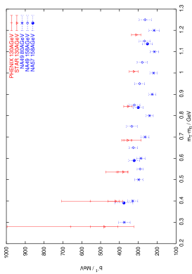
Figure 5: Fit parameters for the $\Lambda$ spectra

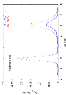
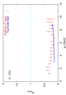
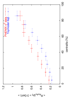
Figure 5: Results for the Toymodel II a $\beta$ with $\Delta E\propto N_{g}\sqrt{E}$ and inhomogeneous energy density distribution

The three diagrams that contribute to the gluon emission amplitude induced by one scattering are depicted in Figure 5. The gluon energy spectrum, which is given by the ratio between the radiation and the elastic cross section, is found to be

$$\omega\frac{\mathrm{d}I}{\mathrm{d}\omega\mathrm{d}^{2}\vec{k}_{\perp}}=N_{c}\frac{\alpha_{s}}{\pi^{2}}\langle\vec{J}(k,q)^{2}\rangle$$ (51)

where $\vec{J}$ is the emission current

$$\vec{J}(k,q)=\frac{\vec{k}_{\perp}}{k_{\perp}^{2}}-\frac{\vec{k}_{\perp}-\vec{q}_{\perp}}{(\vec{k}_{\perp}-\vec{q}_{\perp})^{2}}$$ (52)

and

$$\langle\vec{J}(k,q)^{2}\rangle\equiv\int\!\mathrm{d}^{2}\vec{q}_{\perp}\,\frac{\mu^{2}}{\pi(q_{\perp}^{2}+\mu^{2})^{2}}\vec{J}(k,q)^{2}$$ (53)

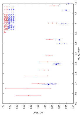
Figure 6: Fit parameters for the $\bar{\Lambda}$ spectra

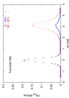
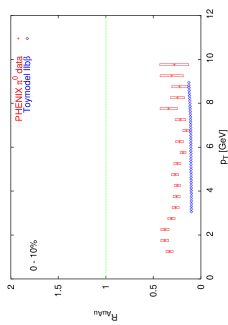
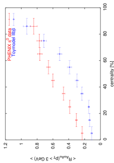
Figure 6: Results for the Toymodel II b $\beta$ with $\Delta E\propto N_{g}^{2}\sqrt{E}$ and inhomogeneous energy density distribution

This result can be generalised to an arbitrary number of scatterings. Figure 6 shows as an example the case of two scatterings.

Figure 6: Gluon emission amplitude induced by two scatterings; $a$, $b$ and $c$ denote the colour indices [25]

The end result becomes quite complicated for a finite number of scatterings and the heuristic discussion is more instructive. Here it is assumed that the number of scatterings is large

$$\frac{1}{N}\ll\kappa\ll 1\qquad\kappa=\frac{\lambda\mu^{2}}{2\omega}$$ (54)

There are three different regimes: the incoherent Bethe-Heitler (BH) regime of small gluon energies, the coherent regime for intermediate $\omega$ and the factorisation limit corresponding to the highest energies. In the BH regime the radiation is due to $N$ incoherent scatterings, in the coherent regime $1/\sqrt{\kappa}$ scatterings act together as a single one (LPM effect) and in the factorisation limit finally all $N$ centres behave as a single scattering centre. This has to do with the formation length of the radiated gluons which increases with the gluon energy. The longer the formation length is the more scatterings occur during the radiation of the respective gluon. The condition 54 can also be expressed in terms of the gluon energy:

$$\omega_{\mathrm{BH}}\sim\lambda\mu^{2}\ll\omega\ll\omega_{\mathrm{fact}}\sim\frac{\mu^{2}L^{2}}{\lambda}\leq E$$ (55)

The last part $\omega_{\mathrm{fact}}\leq E$ is satisfied when the length $L$ of the traversed medium is smaller than the critical length

$$L\leq L_{\mathrm{cr}}=\sqrt{\frac{\lambda E}{\mu^{2}}}$$ (56)

Then the radiation spectrum per unit length is

$$\omega\frac{\mathrm{d}I}{\mathrm{d}\omega\,\mathrm{d}z}\simeq\left\{\begin{array}[]{ll}\frac{\alpha_{s}}{\lambda}&\omega<\omega_{\mathrm{BH}}\\ \frac{\alpha_{s}}{\lambda}\sqrt{\frac{\lambda\mu^{2}}{\omega}}&\omega_{\mathrm{BH}}<\omega<\omega_{\mathrm{fact}}\\ \frac{\alpha_{s}}{L}&\omega_{\mathrm{fact}}<\omega\\ \end{array}\right.$$ (57)

The spectrum can be integrated in the range $0\leq\omega\leq E$ and $0\leq z\leq L$ in order to get the total energy loss. It is found that the energy loss

$$\Delta E(L)\sim\alpha_{s}\frac{\mu^{2}L^{2}}{\lambda}\left(1+O\left(\frac{1}{N}\right)\right)$$ (58)

is proportional to $L^{2}$ and independent of $E$ in the high energy limit. In addition there is a factorisation contribution which is proportional to $\alpha_{s}E$. For the case that $L>L_{\mathrm{cr}}$ or equivalently $E\leq E_{\mathrm{cr}}=L^{2}\mu^{2}/\lambda$ the energy loss becomes

$$\Delta E\simeq\alpha_{s}\sqrt{\frac{\mu^{2}E}{\lambda}}L$$ (59)

Now $\Delta E(L)$ grows only linearly with $L$ but depends on $E$. The different scenarios are reflected in different $E$- and $L$-dependencies of the overall energy loss.

Chapter 5 Experimental Results

1 AGS and SPS

Strangeness Enhancement

A clear enhancement of strangeness is observed in various systems at AGS and SPS. This does not automatically mean that a QGP is formed since the strangeness enhancement can partly result from hadronic interactions [8].

At AGS an increase of the kaon to pion ratio $K/\pi$ is seen and $K^{+}/\pi^{+}>K^{-}/\pi^{-}$. The data are described by purely hadronic models and the strange particle ratios can be fitted by a statistical model with an equilibrated hadronic fireball. This does not mean that the system always was in a hadronic phase [7, 8, 10].

At SPS a global enhancement factor 2 for kaons in central PbPb collisions is observed and again $K^{+}/\pi^{+}>K^{-}/\pi^{-}$. The enhancement increases with the strangeness content of the respective hadron species [7, 15]. The antihyperon ratio $\bar{\Xi}/\bar{\Lambda}$ is found to smoothly increase from pp over pA to AA collisions. Furthermore a strong enhancement of multistrange hadrons from light to heavy nuclei is observed, which can be counted as evidence for a non-hadronic enhancement [7]. Hadronic transport models fail to describe the SPS data unless they invoke non-hadronic scenarios while microscopic transport models are in good agreement with data [7, 8]. The strange particle ratios can be fitted with a hadronic hadron gas and a QGP [7, 8].

This may be seen as evidence for QGP formation, but it has not been possible to unambiguously relate the data on strangeness enhancement to the presence of a QGP. A more detailed discussion of practical and conceptual problems can be found in [7].

Chemical Equilibrium and Freeze-Out

At top AGS and higher energies mid-rapidity particle production can be well described in the framework of a statistical model in full equilibrium while in the integrated results strangeness is undersaturated. The freeze-out points are below the calculated phase boundary for all except the top SPS energy [10].

Charmonium Suppression

$J/\psi$ suppression can be quantified using the ratio of the $J/\psi$ cross section to the cross section for the Drell-Yan process. The Drell-Yan process is the creation of a lepton pair from $q\bar{q}$ annihilation ($q\bar{q}\to l^{+}l^{-}$). It is a hard process that scales with the number of binary nucleon-nucleon collisions in a nucleus-nucleus collision. The ratio $\sigma_{J/\psi}/\sigma_{DY}$ can be interpreted as the probability to produce a $J/\psi$ per binary collision. A big advantage is that many experimental uncertainties drop out in the ratio. It is often given as a function of $L$, the mean length of nuclear matter traversed by a $c\bar{c}$ pair [15]. It is, however, advisable to be careful since this is not a measured quantity and model dependent [7].

$\sigma_{J/\psi}/\sigma_{DY}(L)$ has been measured at CERN for different systems. The results for pA, SU and peripheral PbPb ($L<8\,\mathrm{fm}$) are consistent with the exponential absorption in nuclear environment while in central PbPb ($L>8\,\mathrm{fm}$) a significantly larger suppression is seen [15, 7, 34]. Hadronic transport models reproduce the data but depend heavily on details in the models and need a very high comover density [7, 28] which is not typical for hadronic matter.

The cross section ratio $\sigma_{J/\psi}/\sigma_{DY}(E_{\perp})$ for PbPb collisions as a function of transverse energy shows a clear suppression in addition to the extrapolated absoption in nuclear matter. For peripheral events the data are consistent with the suppression expected from normal absorption, but for mid-central collisions the measured cross section ratio drops significantly below the normal suppression. It continues to decrease for more central events [34].

Additional observations are:

• The loosely bound $\psi^{\prime}$ is similarly absorbed in SU and PbPb [7, 15].

• The statistical hadronisation model describes the centrality dependence of $J/\psi$ at SPS, but only with an increased charm production cross section [19].

• The anomalous $J/\psi$ suppression observed at SPS can be counted as a signal for QGP formation, but there are still many uncertainties and the theoretical debate is far from settled [7, 18].

2 RHIC

At RHIC gold nuclei collide with energies up to 200 GeV per nucleon pair (which corresponds to a total c.m.s. energy of $\sqrt{s}\sim 40\,\mathrm{TeV}$). The energy density reached is expected to be at least a few $\mathrm{GeV/fm^{3}}$ and thus high enough for the formation of a quark-gluon plasma. These calculations are, however, heavily model dependent.

At these centre-of-mass energies, hadrons with high transverse momentum are produced in the fragmentation of partons that underwent a hard scattering. The study of these high-$p_{\perp}$ hadrons is one of the main goals of the four experiments PHENIX, STAR, BRAHMS and PHOBOS.

The particle multiplicities are so high in ion-ion collisions that jets cannot be identified with the normal algorithms which search for a large energy deposition in neighboring calorimeter cells. Instead only single high-$p_{\perp}$ hadrons can be identified and from the relative angle it can be seen whether they belong to the same jet. But since there is a huge background of low-$p_{\perp}$ particles it is impossible to identify also the softer part of the jet and therefore also the total jet energy as well as the jet cone is unknown.

There have also been p+p and d+Au runs at the same energy ($\sqrt{s_{\mathrm{NN}}}=200\,\mathrm{GeV}$) and a Au+Au run at $\sqrt{s_{\mathrm{NN}}}=130\,\mathrm{GeV}$ to which the results can be compared.

1 Suppression of high-$p_{\perp}$ Hadrons

In pp collisions hadrons with $p_{\perp}\gtrsim 2\,\mathrm{GeV}$ are produced in hard scattering processes. If this is also the case in AA collisions the yield of hadrons with large $p_{\perp}$ is expected to scale with the number of binary collisions (Ch. 1). It is therefore often characterised by the ratio $R_{\mathrm{AB}}$ of the yield per nucleon-nucleon collision in AB collisions to the yield in pp collisions:

$$R_{\mathrm{AB}}(p_{\perp},\eta)=\left(\frac{1}{N_{\mathrm{evt}}}\frac{\mathrm{d}^{2}N^{\mathrm{AB}}}{\mathrm{d}p_{\perp}\mathrm{d}\eta}\right)\cdot\left(\frac{\langle N_{\mathrm{coll}}\rangle}{\sigma_{\mathrm{inel}}^{\mathrm{pp}}}\frac{\mathrm{d}^{2}\sigma^{\mathrm{pp}}}{\mathrm{d}p_{\perp}\mathrm{d}\eta}\right)^{-1}$$ (1)

The inelastic pp cross section is from measurements known to be $\sigma_{\mathrm{inel}}^{\mathrm{pp}}\simeq 42\,\mathrm{mb}$ at $\sqrt{s}=200\,\mathrm{GeV}$. $R_{\mathrm{AB}}$ is called the nuclear modification factor since all nuclear effects will lead to a deviation from unity. $\langle N_{\mathrm{coll}}\rangle$ has to be calculated for each centrality class (i.e. range in impact parameter) separately. It should be noted that in the region below $p_{\perp}\simeq 2\,\mathrm{GeV}$ the $p_{\perp}$-spectrum is dominated by hadrons that were produced in soft interactions. This contribution is naively expected to scale with the number of participants rather than the number of binary collisions. This means that even without any nuclear effects $R_{\mathrm{AB}}$ will drop below unity for small $p_{\perp}$. In summary, the nuclear modification factor is a measure of all kinds of nuclear effects and deviations from scaling with $\langle N_{\mathrm{coll}}\rangle$ provided hard scattering processes are the by far dominant source of high-$p_{\perp}$ hadrons.

The nuclear modification factor is measured by all four experiments [35, 36, 37, 38]. There is no need to discuss all of them since the results are similar and therefore only the PHENIX data will be presented here. PHENIX measures charged hadrons and neutral pions covering the pseudorapidity range $|\eta|<0.35$, but for the charged particles a cut of $|\eta|<0.18$ was applied. The events are divided into nine centrality classes that are listed in Table 1 together with the corresponding values of $\langle N_{\mathrm{coll}}\rangle$ and $\langle N_{\mathrm{part}}\rangle$.

Table 1: Centrality classes with the number of participants and binary collisions as used by PHENIX, the percent values characterising the centrality classes give the fraction of the total cross section $\sigma^{\mathrm{AuAu}}=6.9\,\mathrm{b}$ [35]

centrality	$\langle N_{\mathrm{coll}}\rangle$	$\langle N_{\mathrm{part}}\rangle$
$0-10$%	$955.4\pm 93.6$	$325.2\pm 3.3$
$10-20$%	$602.6\pm 59.3$	$234.6\pm 4.7$
$20-30$%	$373.8\pm 39.6$	$166.6\pm 5.4$
$30-40$%	$219.8\pm 22.6$	$114.2\pm 4.4$
$40-50$%	$120.3\pm 13.7$	$74.4\pm 3.8$
$50-60$%	$61.0\pm 9.9$	$45.5\pm 3.3$
$60-70$%	$28.5\pm 7.6$	$25.7\pm 3.8$
$70-80$%	$12.4\pm 4.2$	$13.4\pm 3.0$
$80-92$%	$4.9\pm 1.2$	$6.3\pm 1.2$
min. bias	$257.8\pm 25.4$	$109.1\pm 4.1$

The charged particle spectrum measured by PHENIX in the pp run does not reach far enough in $p_{\perp}$, so the pp reference spectrum was constructed from the $\pi^{0}$ spectrum measured by PHENIX and the observed charged hadron to neutral pion ratio (PHENIX and other experiments [35]).

Figure 1: $R_{\mathrm{AuAu}}(p_{\perp})$ for $\pi^{0}$ and charged hadrons at mid-rapidity for the different centrality classes measured by PHENIX [35]

The results for $R_{\mathrm{AuAu}}$ at $\sqrt{s_{\mathrm{NN}}}=200\,\mathrm{GeV}$ are shown in Figure 1. There is a clear suppression of high-$p_{\perp}$ hadrons that gradually increases with increasing centrality. The event centrality is determined from the number of spectator neutrons and the number of fast secondaries. The drop in the region $p_{\perp}\lesssim 2\,\mathrm{GeV}$ is certainly caused at least partly by the $\langle N_{\mathrm{coll}}\rangle$ instead of $\langle N_{\mathrm{part}}\rangle$ scaling in Equation 1. The ratio is flat for $p_{\perp}\gtrsim 4.5\,\mathrm{GeV}$ indicating that particle production is dominated by hard scattering in this regime although the yield per binary collision is not as high as in pp collisions. The scaling with $x_{\perp}$ ($x_{\perp}=2p_{\perp}/\sqrt{s}$) gives further support to this hypothesis [35]. The increase of the suppression with centrality is consistent with a plasma scenario since the size and thereby the energy loss suffered by hard partons are also expected to increase with centrality. From the Cronin effect an enhancement of particles with intermediate $p_{\perp}$ (Ch. 5) is expected so that the suppression is possibly even higher.

It has been argued in [39] that in case of plasma formation and high energy loss in the deconfined medium only the partons produced near the surface could escape since they would be thermalised if the way through the plasma was too long. This would result in a scaling with $\langle N_{\mathrm{part}}\rangle$ instead of $\langle N_{\mathrm{coll}}\rangle$ also for the high-$p_{\perp}$ hadrons [39]. There is, however, no clear evidence for that.

A surprising result is the centrality dependence of the nuclear modification factor: It scales neither with $\langle N_{\mathrm{coll}}\rangle$ nor with $\langle N_{\mathrm{part}}\rangle$ but is linear as a function of percent of the total cross section. Figure 2 shows the centrality dependence of the mean $R_{\mathrm{AuAu}}$ for $p_{\perp}>3\,\mathrm{GeV}$ of the PHENIX $\pi^{0}$ data, the linear fit is

$$\langle R_{\mathrm{AuAu}}(p_{\perp}>3\,\mathrm{GeV})\rangle=(0.00835\pm 0.00034)\cdot\mathrm{centrality\ [\%]}+(0.186\pm 0.012)$$ (2)

There is no convincing explanation for this behaviour so far.

Figure 2: Centrality dependence of the mean $R_{\mathrm{AuAu}}$ for $p_{\perp}>3\,\mathrm{GeV}$ for PHENIX $\pi^{0}$ data [51]

Figure 3: Charged hadron to neutral pion ratio in central ($0-10\%$ - squares) and peripheral ($80-92\%$ - circles) AuAu collisions (the peripheral data points are offset by 130 MeV); PHENIX [42]

Figure 4: $p/\pi$ (left) and $\bar{p}/\pi$ (right) ratios; open (filled) points are for charged (neutral) pions; PHENIX [42]

An astonishing feature of Figure 1 is the stronger suppression of neutral pions at intermediate $p_{\perp}$. It turns out that this is not a stronger suppression of $\pi^{0}$ but a higher production rate of protons and antiprotons. Figure 3 shows the ratio of charged hadrons to neutral pions in AuAu for central and peripheral collisions. The dotted line at 1.6 indicates the ratio measured in $e^{+}e^{-}$ and pp collisions. This plot nicely illustrates the excess of charged particles at intermediate $p_{\perp}$. From Figure 4 it becomes clear that this is caused by an enhanced (anti)proton production in more central AuAu collisions indicating a deviation from the standard picture of particle production in the medium-$p_{\perp}$ range ($2\,\mathrm{GeV}\lesssim p_{\perp}\lesssim 4.5\,\mathrm{GeV}$).

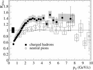
Figure 5: $R_{\mathrm{dAu}}$ for charged hadrons and neutral pions at $\sqrt{s_{\mathrm{NN}}}=200\,\mathrm{GeV}$; PHENIX [40]

In deuteron-gold collisions at RHIC no suppression of high-$p_{\perp}$ hadrons is observed. At mid-rapidity there is an enhancement [37, 40, 41] that is usually interpreted as the Cronin effect while the ratio is consistent with unity at larger rapidities [43]. This further strengthens the case for a plasma scenario since the suppression in AuAu collisions is obviously related to final state effects (initial state effects should be present in the dAu data as well). Figure 5 shows the nuclear modification factor $R_{\mathrm{dAu}}$ in dAu collisions measured by PHENIX, the values of $\langle N_{\mathrm{coll}}\rangle$ and $\langle N_{\mathrm{part}}\rangle$ are 8.5 and 1.7 respectively.

In summary, there is a substantial suppression of high-$p_{\perp}$ hadrons in AuAu collisions that smoothly increases with increasing centrality. The spectral shape is unchanged as compared to pp for large $p_{\perp}$ indicating that fragmentation of hard partons is the dominant particle production mechanism in this regime. At medium $p_{\perp}$ a large relative proton and antiproton yield is observed, which is a hint to a deviation from the ”normal” particle production. All observables approach their pp values in the most peripheral events. It should be kept in mind that the scaling behaviour is different for small $p_{\perp}$. No suppression is observed in dAu collisions indicating final state effects as the most probable origin. These results are consistent with a scenario where a quark-gluon plasma is formed in the overlap region of the colliding nuclei and energetic partons lose a substantial amount of energy when traversing the plasma. However, this is an indication and no proof.

Surprisingly the nuclear modification factor increases linearly with centrality, this feature is presently not understood.

2 Disappearance of Back-to-Back Hadron Correlations

STAR also measures the azimuthal correlation of charged particles at mid-rapidity ($|\eta|<0.7$) [41, 44]. The azimuthal distribution is defined as

$$D(\Delta\phi)=\frac{1}{N_{\mathrm{trig}}}\frac{\mathrm{d}N}{\mathrm{d}(\Delta\phi)}$$ (3)

Particles with $4<p_{\perp}<6\,\mathrm{GeV}$ are defined as trigger particles. For each trigger particle the azimuthal separation $\Delta\phi$ from all other particles satisfying $2\,\mathrm{GeV}<p_{\perp}<p_{\perp}(\mathrm{trig})$ is calculated yielding $N(\Delta\phi)$. In pp collisions $D(\Delta\phi)$ shows clear jet-like peaks at $\Delta\phi\sim 0$ and $\Delta\phi\sim\pi$ (Fig. 6 and 7(a)). The distribution is characterised by a Gaussian for each peak:

$$D(\Delta\phi)=\frac{A_{N}}{\sqrt{2\pi}\sigma_{N}}e^{-(\Delta\phi)^{2}/2\sigma_{N}^{2}}+\frac{A_{B}}{\sqrt{2\pi}\sigma_{B}}e^{-(|\Delta\phi|-\pi)^{2}/2\sigma_{N}^{2}}+P$$ (4)

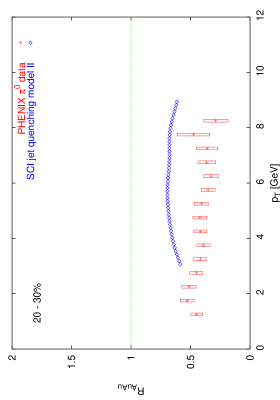
Figure 7: Model results for the nuclear modification factor with non-uniform energy density for different centrality classes and PHENIX data [51]

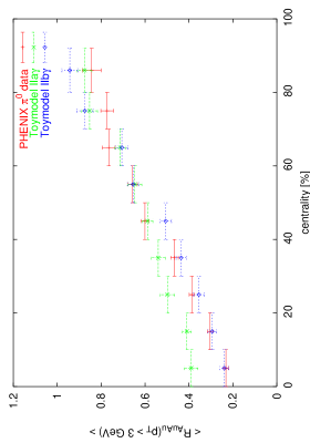
Figure 7: Centrality dependence of $R_{\mathrm{AuAu}}$ for the Toymodel II a $\gamma$ with $\Delta E\propto N_{g}$ and Toymodel II b $\gamma$ with $\Delta E\propto N_{g}^{2}$, both with non-uniform energy density profile

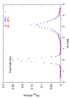
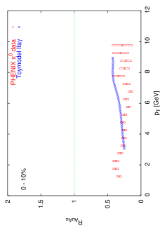
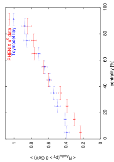
Figure 7: Results for the Toymodel II a $\gamma$ with $\Delta E\propto N_{g}$ and inhomogeneous energy density distribution

where the indices $N$ and $B$ stand for the near-side and back-to-back respectively and $P$ is a constant offset. The fit is shown as the solid line in Figure 7(a), the parameters are given in Table 2.

Table 2: Fit parameters from Equation 4, for the AuAu central sample only one Gaussian was fitted to the data after subtraction of the flow and pedestal contribution [41]

	pp min. bias	dAu min. bias	AuAu central
$A_{N}$	$0.081\pm 0.005$	$0.074\pm 0.003$	$0.093\pm 0.008$
$\sigma_{N}$	$0.18\pm 0.01$	$0.20\pm 0.01$	$0.22\pm 0.02$
$A_{B}$	$0.119\pm 0.007$	$0.097\pm 0.004$	$\diagup$
$\sigma_{B}$	$0.45\pm 0.03$	$0.48\pm 0.02$	$\diagup$
$P$	$0.008\pm 0.001$	$0.039\pm 0.001$	$0.004\pm 0.003$

In nucleus-nucleus collisions there will also be a contribution from the elliptic flow anistropy (Ch. 4):

$$\frac{\mathrm{d}N_{\mathrm{ef}}}{\mathrm{d}(\Delta\phi)}=B[1+2v_{2}^{2}\cos(2\Delta\phi)]$$ (5)

where $v_{2}$ has been measured independently in the same set of events and is assumed to be constant in $2<p_{\perp}<6\,\mathrm{GeV}$, whereas $B$ has to be fitted. The values for the different centrality classes are listed in Table 3.

Table 3: Values of $N_{\mathrm{part}}$, $v_{2}$ ($2<p_{\perp}<6\,\mathrm{GeV}$) and the normalisation constant $B$ for the different centrality classes [44]

centrality	$N_{\mathrm{part}}$	$v_{2}$	$B$
0-5%	$352\pm 7$	$0.07\pm 0.01$	$1.442\pm 0.003$
5-10%	$298\pm 10$	$0.10\pm 0.01$	$1.187\pm 0.008$
10-20%	$232\pm 11$	$0.15\pm 0.01$	$0.931\pm 0.006$
20-30%	$165\pm 13$	$0.19\pm 0.01$	$0.633\pm 0.005$
30-40%	$144\pm 13$	$0.21\pm 0.01$	$0.420\pm 0.005$
40-60%	$61\pm 10$	$0.22\pm 0.01$	$0.231\pm 0.003$
60-80%	$20\pm 6$	$0.24\pm 0.04$	$0.065\pm 0.003$

\psfrag{Delta phi}{$\Delta\phi\ [\mathrm{rad}]$}\psfrag{D(Delta phi)}{$D(\Delta\phi)$}\includegraphics[scale={0.8}]{plots/D2.eps}

Figure 6: Azimuthal distribution $D(\Delta\phi)$ for pp and different centralities in AuAu measured by STAR, the lines show the elliptic flow and pedestal contribution (Eq. 5,Tab. 3) [44]

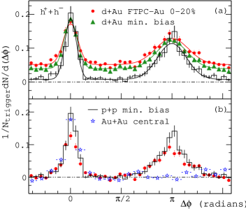
Figure 7: Azimuthal distribution $D(\Delta\phi)$ for pp, dAu and central AuAu (elliptic flow and pedestal distributions have been subtracted in (b)), solid lines in (a) are Gaussian fits (Eq. 4, Tab. 2), STAR [41]

Figure 6 shows the measured azimuthal distribution for different centralities in AuAu together with the elliptic flow contribution (solid lines) and the pp data. Jet-like correlations can be seen as an excess of the measured correlation over the elliptic flow contribution. The jet on the trigger side ($\Delta\phi\sim 0$) is present for all centralities but the away-side jet ($\Delta\phi\sim\pi$) vanishes in more central events. In Figure 7(b) the distribution in pp collisions is compared to central AuAu collisions after subtraction of the elliptic flow and pedestal contributions. It is not surprising that the correlation on the trigger side is nearly as strong as in pp collisions since the trigger condition introduces a bias. The important point is that the jet on the other side disappears completely in the most central collisions. The suppression increases again smoothly with centrality.

The results from the dAu measurements are shown in Figure 7(a) and Table 2. There is no substantial suppression of the away-side jet which again points towards final state effects being responsible for the disappearance of the second jet in central AuAu collisions.

The results are commonly interpreted in terms of a plasma scenario in the following way. The data samples for the AuAu collisions are heavily biased towards events where the hard scattering took place near the surface of the overlap region due to the trigger condition. Particles with $p_{\perp}>4\,\mathrm{GeV}$ are rare already in pp collisions. If the energetic parton is produced inside the plasma and has to traverse a substantial part of it, it will lose a sizable fraction of its energy in interactions with the plasma. The leading hadron formed in the fragmentation will then have a transverse momentum which is too small to pass the trigger condition. If now the hard scattering happened near the surface with one parton escaping undisturbed the other one will typically have to traverse a substantial part of the plasma for geometrical reasons. The mean path length through the plasma increases with increasing centrality and one would therefore expect an increasing suppression of the away-side jet. In dAu collisions, where no plasma is formed, the azimuthal correlation should be similar to pp distribution.

This argumentation sounds convincing, nevertheless one has to be careful. Firstly the $p_{\perp}$-spectrum has a tail to very high energies and these partons may produce trigger particles even after heaving lost some energy. Therefore the trigger bias does not automatically mean that the hard scattering took place near the surface. This point can only be clarified with the number of trigger particles produced per binary collision which is much smaller in the scenario where only scatterings that happen to be located near the surface can give rise to trigger particles. Secondly the lifetime of the QGP which is estimated to be of the order of a few fm limits the path lengths. In the surface emission scenario this would lead to saturation as soon as the geometrically available path length becomes shorter than the lifetime. And finally the matrix element is symmetric in azimuth which means that there is a sizable probability that both partons escape nearly undisturbed when they are emitted from the surface. Consequently the observed azimuthal correlation seems to contradict the surface-emission scenario and the observed jets stem from some greater depth.

The conclusion can be drawn that also the measured azimuthal correlation of high-$p_{\perp}$ hadrons is qualitatively consistent with the hypothesis of quark-gluon plasma being formed in relativistic nucleus-nucleus collisions.

3 Correlation with the Reaction Plane

The almond-like shape of the overlap region in mid-central collisions leads to a dependence of the two-particle correlation (Eq. 3) on the orientation of the pair relative to the reaction plane. A parton that is emitted in the reaction plane has on average to traverse a shorter distance in the QGP than one that is emitted perpendicular to it. Consequently the suppression of the away-side jet is stronger in the latter case.

The effects of different emission angles with respect to the reaction plane have alse been studied by the STAR experiment [45]. The procedure is analogous to the one described in Section 2 but here all tracks with $|\eta|<1$ are considered. A pair is defined to be in-plane if the azimuthal angle of the trigger particles satisfies $|\phi^{\mathrm{trig}}-\Psi_{2}|<\pi/4$ or $|\phi^{\mathrm{trig}}-\Psi_{2}|>3\pi/4$ where $\Psi_{2}$ is the reaction plane angle of the event. A trigger is out-of-plane if $\pi/4<|\phi^{\mathrm{trig}}-\Psi_{2}|<3\pi/4$.

The elliptic flow contribution is [45]

$$\frac{\mathrm{d}N_{\mathrm{out}}^{\mathrm{in}}}{\mathrm{d}\Delta\phi}=B\left[1+2v_{2}^{\mathrm{assoc}}\left(\frac{\pi v_{2}^{\mathrm{trig}}\pm 2\langle\cos(2\Delta\Psi)\rangle}{\pi\pm 4v_{2}^{\mathrm{trig}}\langle\cos(2\Delta\Psi)\rangle}\right)\cos(2\Delta\phi)\right]$$ (6)

where $v_{2}^{\mathrm{assoc}}$ and $v_{2}^{\mathrm{trig}}$ are the elliptic flow of the associated and trigger particles, respectively, and $\langle\cos(2\Delta\Psi)\rangle$ is the reaction plane resolution. The values for 20%-60% centrality are $v_{2}^{\mathrm{assoc}}=0.20$, $v_{2}^{\mathrm{trig}}=0.18$ and $\langle\cos(2\Delta\Psi)\rangle=0.70$.

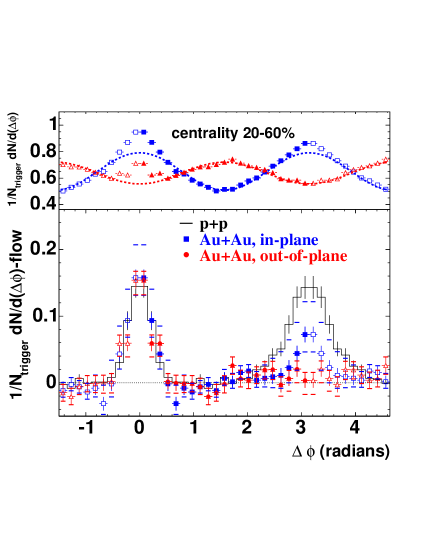
Figure 8: Upper panel: Two-particle correlations for trigger particles in-plane (squares) and out-of-plane (triangles) in mid-central AuAu. The contribution from elliptic flow is shown by dashed lines. Lower panel: Azimuthal distributions after subtracting the elliptic flow and pp data.[45]

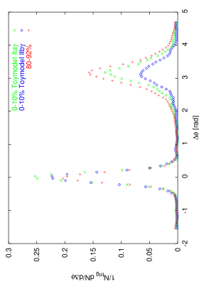
Figure 8: 2-particle azimuthal correlation for the Toymodel II a $\gamma$ with $\Delta E\propto N_{g}$ and Toymodel II b $\gamma$ with $\Delta E\propto N_{g}^{2}$, both with non-uniform energy density profile, the 80-92% data are the same in both cases

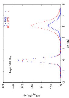
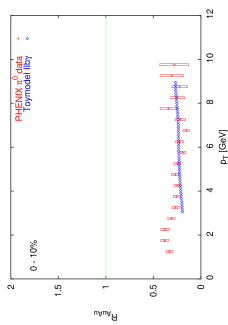
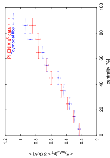
Figure 8: Results for the Toymodel II b $\gamma$ with $\Delta E\propto N_{g}^{2}$ and inhomogeneous energy density distribution

The azimuthal distributions are shown in the upper panel of Figure 8. The solid symbols are data points whereas the open symbols are reflections around $\Delta\phi=0$ and $\Delta\phi=\pi$. The elliptic flow contributions from Equation 6 were fitted with $B$ as the only free parameter. The results, shown as dashed lines, are $B=0.649\pm 0.004(stat.)\pm 0.005(sys.)$ for the in-plane and $B=0.638\pm 0.004(stat.)\pm 0.002(sys.)$ for the out-of-plane distribution.

The lower panel of Figure 8 shows the distributions after subtraction of the elliptic flow together with the pp measurement. The data clearly confirm a stronger quenching of jets perpendicular to the reaction plane where the original parton had to travel a longer distance inside the QGP and thus experienced larger energy loss. The large uncertainty is mainly due to the uncertainty in the elliptic flow contribution.

The fact that a substantial part of the away-side jets survives in the reaction plane also illustrates that the QGP cannot be completely opaque since the smallest diameter of the overlap region in a 20% centrality event is already $\sim 4\,\mathrm{fm}$. It can thus be concluded that a considerable part of the jets survives a journey of a few fm through the QGP.

4 Other Observables

The yields of multi-strange particles are enhanced as compared to SPS. The data indicate strangeness saturation for central collisions [46].

The particle ratios are again beautifully described by a statistical model assuming full chemical equilibrium. The freeze-out point is found to be consistent with the phase boundary calculated with lattice QCD [47]. Furthermore it has been shown that the chemical freeze-out temperature coincides with the critical temperature since it is not possible to maintain chemical equilibrium in a hadronic phase even close to the phase transition [48]. This provides a strong argument for QGP formation.

The first measurements of $J/\psi$ production show a suppression but the experimental uncertainty (mainly lack of statistics) is still too large to make more detailed statements [49].

Chapter 6 Comparison of Identified Particle Spectra from SPS and RHIC

While the hard part of the $p_{\perp}$-spectra in nucleon-nucleon collisions is theoretically under control and shows the power-law behaviour typical for hard parton-parton scattering this is not the case for the soft part. Here the main contribution comes from non-perturbative processes that are not well understood so that one has to rely on paramtrisations of measured cross sections. However, the situation is not as bad in ion-ion collisions where the soft part of the $p_{\perp}$-spectra is better understood and contains valuable information about the properties of the created medium.

In collisions of relativistic nuclei the low-$p_{\perp}$ part of the hadron spectra is determined by the hydrodynamic behaviour of the system, primarily the freeze-out temperature and the pressure which drives the transverse expansion. A still open question is whether the physics at SPS energies is qualitatively different from the physics at RHIC. The hard part of the spectra is hardly accessible at SPS, but the soft part can be used to quantify differences between RHIC and SPS. In this chapter a detailed comparison of the shapes of the $p_{\perp}$- spectra of identified particles is carried out.

A thermal source at rest emitting particles from the origin leads to a spectrum of the form

$$\frac{\mathrm{d}^{2}N}{m_{\perp}\mathrm{d}m_{\perp}\mathrm{d}y}\propto e^{-\frac{m_{\perp}-m_{0}}{T}}$$ (1)

which is completely determined by the temperature. $m_{\perp}=\sqrt{p_{\perp}^{2}+m_{0}^{2}}$ is the transverse mass and $m_{0}$ is the respective particle’s rest mass. The transverse expansion leads to deviations from this form which are, however, model dependent. Further distortions arise from resonance decays.

The freeze-out temperature can be extracted from the ratios of different particle yields and is found to be nearly the same for SPS and RHIC, namely $T=(168\pm 2.4)\,\mathrm{MeV}$ at SPS [50] and $T=(174\pm 7)\,\mathrm{MeV}$ at RHIC [47]. Differences in the shape of the spectra should thus stem from different expansion velocities.

In order to avoid the problem with the model dependence of the transverse expansion contribution an exponential $a\exp{\{-b(m_{\perp}-m_{0})\}}$ is fitted locally, i.e. in a small $p_{\perp}$-interval, to the $p_{\perp}$-spectrum. $b$ will then depend on $p_{\perp}$ and cannot be interpreted as an inverse temperature, but it can be used to quantify differences in the slopes of the spectra. Since this comparison relies solely on the shape of the spectrum the parameter $a$ which describes the yields is irrelevant. To get comparable results the spectra from central collisions near mid-rapidity were used. A large number of different identified particle spectra were analysed in order to improve the significance and give an overview over the present status in terms of experimental data. All analysed spectra are listed in Table 1. Concerning protons and antiprotons only spectra that are corrected for feed-down from week decays were considered. Figure 1 shows as an example a measured pion spectrum with the fitted exponentials.

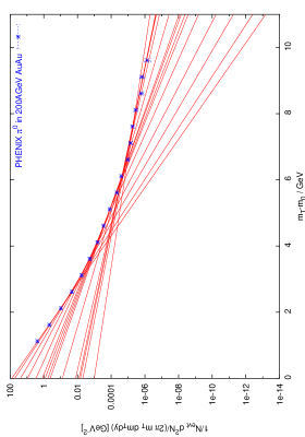
Figure 1: $\pi^{0}$ spectrum measured by the PHENIX experiment [51] with locally fitted exponentials

A potentially critical point is the possible dependence of the results on the interval length. Fortunately it was found be small as is illustrated in Figure 2. A compromise between a small interval, which is desirable because of better sensitivity and resolution, and a small error has to be made. The interval length was therefore chosen individually for each spectrum depending mainly on the experimental uncertainties.

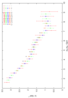
Figure 2: Fit parameters for the $\pi^{0}$ spectrum from Figure 1 obtained with different interval lengths

The results for the kaons are shown in Figure 3 as a representative, the rest can be found in Appendix 12. The fact that $b$ changes with $p_{\perp}$ illustrates that transverse expansion does indeed play a role. The differences between SPS and RHIC are small, the RHIC points are continuously slightly higher. The discrepancies among the experiments at the same accelarator are also sizable, in fact they are of the same magnitude as the differences between RHIC and SPS. There is also no visible difference between the SPS data at 80 A GeV and 158 A GeV beam energy, except maybe in the $\Lambda$ spectra. The sum of the results clearly suggests that there is no dramatic change in (soft) physics when going from SPS to RHIC. There is room for a small quantitative difference.

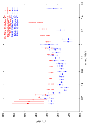
Figure 3: Fit parameters for the kaon spectra

A comparison of the elliptic flow leads to the same conclusion, here the differences between SPS and RHIC are also not very big. Indeed the two observables are correlated because the pressure, that drives the transverse expansion, also has an influence on the pressure gradient, which is responsible for the elliptic flow. The transverse size of the system also turned out to be similar at SPS and RHIC [52]. Together these observation lend even stronger support to the conclusion that at least the soft physics is similar at SPS and RHIC.

Table 1: List of all analysed spectra

Particle	Experiment	Energy	System	# points	Centrality
		[A GeV]		per fit
$K^{+}$	PHENIX	200	Au+Au	5	5.0%	[53]
$K^{-}$	PHENIX	200	Au+Au	5	5.0%	[53]
$K^{+}$	STAR	200	Au+Au	6	5.0%	[54]
$K_{s}$	NA57	158	Pb+Pb	4	4.5%	[55]
$K^{+}$	NA44	158	Pb+Pb	6	3.7%	[56]
$K^{+}$	NA49	158	Pb+Pb	5	5.0%	[57]
$\Lambda$	PHENIX	130	Au+Au	4	5.0%	[58]
$\Lambda$	STAR	130	Au+Au	4	5.0%	[59]
$\Lambda$	NA49	80	Pb+Pb	6	7.2%	[60]
$\Lambda$	NA49	158	Pb+Pb	7	10.0%	[60]
$\Lambda$	NA57	158	Pb+Pb	4	4.5%	[55]
$\bar{\Lambda}$	PHENIX	130	Au+Au	5	5.0%	[58]
$\bar{\Lambda}$	STAR	130	Au+Au	4	5.0%	[59]
$\bar{\Lambda}$	NA49	80	Pb+Pb	4	7.2%	[60]
$\bar{\Lambda}$	NA49	158	Pb+Pb	4	10.0%	[60]
$\bar{\Lambda}$	NA57	158	Pb+Pb	4	4.5%	[55]
$p$	PHENIX	200	Au+Au	5	5.0%	[53]
$p$	NA44	158	Pb+Pb	6	3.7%	[56]
$p$	NA49	80	Pb+Pb	5	7.0%	[61]
$p$	NA49	158	Pb+Pb	6	10%	[61]
$\bar{p}$	PHENIX	200	Au+Au	5	5.0%	[53]
$\bar{p}$	NA44	158	Pb+Pb	7	3.7%	[56]
$\bar{p}$	NA49	80	Pb+Pb	7	7.2%	[61]
$\bar{p}$	NA49	158	Pb+Pb	7	10.0%	[61]
$\pi^{0}$	PHENIX	200	Au+Au	5	10.0%	[51]
$\pi^{+}$	PHENIX	200	Au+Au	5	5.0%	[53]
$\pi^{+}$	STAR	200	Au+Au	5	5.0%	[54]
$\pi^{+}$	NA44	158	Pb+Pb	8	3.7%	[56]
$\pi^{\pm}$	NA45	158	Pb+Au	5	6.1%	[62]
$\pi^{-}$	NA49	158	Pb+Pb	5	5.0%	[57]
$\pi^{0}$	WA98	158	Pb+Pb	5	10% of min.bias	[63]

Chapter 7 Monte Carlo Techniques

A very general definition would be that Monte Carlo is everything that makes use of random numbers to solve a problem. Monte Carlo methods are mainly used to simulate processes, estimate integrals or select random variables according to some probability density (or a combination of these). The processes to which Monte Carlo methods are applicable do not necessarily have to be of stochastic nature, although this is normally the case in high energy physics.

The values that a random variable takes are unpredictable, so there have to be at least two different possible values of that variable. The distribution of a random variable is given by a probability density $g(u)\mathrm{d}u$, which is the probability that the value lies in the range $[u,u+\mathrm{d}u]$. The scattering angle in a $a+b\to a+b$ elastic scattering is an example for a random variable. In this case the probability density is given by the differential cross section $\mathrm{d}\sigma=f(\vartheta)\mathrm{d}\vartheta$. This example also illustrates that probability densities in physical problems are often not normalised to unity, because the integral may also have a physical meaning (in this example the total cross section).

The integral of a function $f(x)$ in an interval $[a,b]$ can be estimated by choosing $N$ values $x_{i}$ distributed randomly in $[a,b]$, summing the function values $f(x_{i})$ in these points and dividing by $N$. According to the law of large numbers the Monte Carlo estimate of an integral converges (in the statistical sense) to its exact value as the number of points approaches infinity.

$$\frac{1}{N}\sum_{i=1}^{N}f(x_{i})\stackrel{{\scriptstyle N\to\infty}}{{\longrightarrow}}\frac{1}{b-a}\int\limits_{a}^{b}\!\mathrm{d}x\,f(x)$$ (1)

Convergence in the statistical sense means that for every probability $p$ and positive number $\epsilon$ there is a $k$ such that for all $N>k$ the probability of the difference between the left- and the right-hand side of Equation 1 being smaller than $\epsilon$ is greater than $p$.

The Monte Carlo estimate is a function of the random numbers $\{x_{i}\}$. For finite $N$ the value obtained with a different set of numbers $\{x^{\prime}_{i}\}$ will be different from the first one. The central limit theorem says that for large $N$ the Monte Carlo estimate is a Gaussian distribution. Its expectation is the true value of the integral. The expectation of a function $f(x)$ is defined as

$$E(f)=\int\!\mathrm{d}x\,f(x)g(x)$$ (2)

and the variance (average of the squared deviation from the expectation) is

$$V(f)=E[(f-E(f))^{2}]=\int\!\mathrm{d}x\,(f-E(f))^{2}g(x)$$ (3)

The variance of the Monte Carlo estimate is $V(f)/N$. The speed, with which the Monte Carlo estimate converges, does not depend explicitly on the number of dimensions (although other calculations in the algorithm might take more time in higher dimensions). This means that for small number if dimensions numerical quadrature will be much more efficient while the Monte Carlo clearly wins for higher number of dimensions. Since the variance also depends on the variance of the function $f$, the performance of the Monte Carlo can also be improved by reducing $V(f)$. These methods will not be discussed explicitly here but can be found for example in [64]. The variance reducing techniques described below for the selection from a given probability density can be adopted to the estimation of integrals.

Given a random number generator that produces numbers $R$ uniformly distributed in $]0,1[$ these can be used to obtain numbers distributed according to any other density function $f(x)$ defined on an interval $[a,b]$. This is extremely useful in simulations of physical processes.

The simplest way to do that is the hit-or-miss Monte Carlo. First an upper limit $f_{\mathrm{max}}$ of the function has to be found, i.e. $f_{\mathrm{max}}\geq f(x)\ \forall x\in[a,b]$. Then the procedure is to select an $x$ from a flat distribution, i.e. $x=a+R(b-a)$ where $R$ is a random number in $]0,1[$. Then another random number $R$ in the interval $]0,1[$ is selected and if $R<f(x)/f_{\mathrm{max}}$ the $x$-value is accepted. Otherwise it is rejected and the procedure continues with choosing a new $x$.

The advantage of this algorithm is that it works for practically all functions without singularities. The efficiency is

$$\frac{\int\!\mathrm{d}x\,f(x)}{f_{\mathrm{max}}(b-a)}$$ (4)

If $f$ varies a lot the efficiency becomes very bad, so it might be useful to divide the interval into suitable subintervals. Then a decision which subinterval to choose has to be made first (the relative probability is given by the integral in the subinterval).

Another method is the direct sampling, that can be used if $f$ has a primitive function $F$ whose inverse $F^{-1}$ can be calculated. Then $x$-values can be found using the relation

$$\int\limits_{a}^{x}\!\mathrm{d}x^{\prime}\,f(x^{\prime})=R\int\limits_{a}^{b}\!\mathrm{d}x\,f(x)$$ (5)

$$\Rightarrow x=F^{-1}(F(a)+R(F(b)-F(a)))$$ (6)

This is a very elegant and efficient method with the main drawback that the number of functions to which it can be applied is very limited.

The efficiency can also be improved by generating more points in regions where the function values are large (importance sampling). This is mathematically equivalent to a change of integration variable:

$$f(x)\mathrm{d}x=\frac{f(x)}{g(x)}\mathrm{d}G(x)\quad\mathrm{where}\quad\mathrm{d}G(x)=g(x)\mathrm{d}x$$ (7)

In practice it works like this: First a suitable function $g(x)$ has to be chosen. Suitable means that it satisfies (i) $g(x)\geq f(x)\,\forall x\in[a,b]$, (ii) has an invertible primitve function or a $g$-distributed random number generator is available and (iii) the ratio $f(x)/g(x)$ should be as constant as possible. Then select a $x$ according to $g(x)$. Then a random number $R$ is selected, the corresponding $x\in[a,b]$ is accepted if $R<f(x)/g(x)$ and rejected otherwise. The importance sampling will improve the efficiency if $V(f/g)<V(f)$, but it suffers from the small number of available functions $g$.

A crucial point in all Monte Carlo calculations or simulations is the random number generator, since reliable random numbers are needed. Truly random numbers are unpredictable and therefore also unreproducible. They can be obtained from physical processes such as radioactive decay or thermal noise in an electronic circuit. However, these truly random numbers have some disadvantages when it comes to their application. One point is that it is difficult to construct a device that generates random numbers by observing suitable processes being at the same time accurate and very fast. In fact speed is of great importance, since extended simulations consume huge amounts of random numbers.

An alternative to using truly random numbers is to generate pseudo-random numbers from a mathematical formula. These are not random in the sense that they are reproducible, but are just as good for Monte Carlo calculations as long as they are uncorrelated (which is of course the critical point). There are also advantages in the sequence of numbers generated being always the same for one particular starting point, e.g. debugging of a program using random numbers becomes much easier. When generated on a computer the sequence of numbers has a finite length and at some point there will be a number that has already occured before. From now on the sequence will repeat itself and therefore be useless. So the period is an important characteristic of a (pseudo-) random number generator. The generator used in this study has a period of over $10^{43}$.

The ideal algorithm for producing pseudo-random numbers does not exist, so testing is an issue. But even with a lot of tests made it is never possible to be sure that the numbers are suitable for a certain problem that is to be investigated using Monte Carlo methods. It should therefore be kept in mind that the generator one is using is not perfect and that problems may occur. The lesson to learn is that random number generators have to be handled with care.

Monte Carlo event generators are powerful tools for the simulation of complicated processes like particle collisions, where one has to deal with many degrees of freedom. Instead of trying to solve the whole problem in one step (which is practically impossible), the process is divided into a sequence of subprocesses each of which is of reasonable complexity. For high energy physics, for instance, the first part consists of the particles before the interaction, where they are treated in terms of their parton density functions. The next step is the hard interaction that can be calculated using pQCD matrix elements. Then parton showers à la DGLAP are added, after that the event is hadronised and as a last step follows the decay of unstable particles. In each part the dynamical variables are chosen from their probability distributions. The outcome of this whole machinery is a list of all particles in the final states with their masses and momenta, but also the complete history of the event is provided. When generating many events the cross sections can be estimated at the same time. Ideally the mean and variance of a sample of generated events should be the same as for the real physical process.

For this study the Pythia 6.2 package [6] was used, but with an additional phase, representing the interaction of the scattered partons with the plasma, added between the generation of parton showers and hadronisation.

Chapter 8 Soft Colour Interactions

As was already discussed in Chapter 1 only QCD processes involving a large momentum transfer can be treated in pertubation theory, since the coupling strength $\alpha_{s}$ increases with decreasing energy. This is exactly the reason why it cannot be assumed that interactions below the cutoff for perturbative calculations do not occur. They may be negligible in many situations but there are observables related to the hadronic final state that are sensitive to the soft interactions.

The Soft Colour Interaction (SCI) model [1] is an attempt to gain a better understanding of non-pQCD (non-perturbative QCD) processes. It describes the interaction of partons originating from a hard scattering in $ep$ or $p\bar{p}$ collisions with the colour background field inside the hadron. The basic assumption is that the change in the dynamics caused by the soft interactions is negligible. The important point is that the partons can exchange colour leading to a different string topology, which may then result in a different final state after hadronisation of the string.

The background field is represented by the remnants of the hadron(s), i.e. those consituents that did not take part in the hard scattering (Ch. 1). In the case where a valence quark was kicked out the remainder is a diquark in a colour antitriplet state. If the scattered parton is a gluon the remnant (namely the three valence quarks in a colour octet state) is split into a quark and a diquark. If a seaquark was scattered its partner has to be taken into account to conserve quantum numbers. The remnant then consists of the three valence quarks (again split into a quark and a diquark) and the seaquark partner. Together they form a (anti)triplet, depending on whether the seaquark or the sea-antiquark is left.

The interactions consist of an exchange of a colour octet (consisting of colour and anticolour) between a pair of partons, i.e. this can be viewed as a soft gluon exchange. The model is implemented as add-on routines to Pythia at a stage between the hard scattering process including parton showers and the hadronization. Each perturbativly produced parton may interact with each of the remnant consituents with a probability $P_{\mathrm{int}}$ which cannot be calculated from theory and is the only free parameter of the model. The outcome of this procedure will vary from event to event.

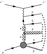
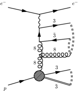
Figure 1: Photon-gluon fusion in deep inelastic scattering with the strings drawn as double dashed lines; left: configuration in the Lund model, right: configuration after the exchange of a soft gluon (colour octet) between the quark from the $2\to 2$ scattering and the quark in the remnant [1].

One example for a deep inelastic scattering event is shown in Figure 1. In the conventional Lund model the remnant is in a colour octet state with the colour and anticolour charges matching those of the gluon so that gluon and remnant together form a singlet. In the case shown in Figure 1 the radiated gluon carries the anticolour charge of the original gluon (which belongs to the charge of the quark in the remnant) and its colour is the anticolour of the original gluon after the radiation. When this gluon splits into a $q\bar{q}$ pair the quark gets the colour and the antiquark the anticolour charge resulting in the string configuration shown in Figure 1. The exchange of a soft gluon between the two quarks in the diagram leads to an interchange of the two colour charges resulting in a different string topology (right-hand side of Figure 1). Now the remnant system is in a singlet state. If instead the antiquark had interacted with the diquark, the scattered quark-antiquark pair would form a colour singlet system and the remnant, together with the radiated gluon, would form the other singlet.

The Generalized Area Law (GAL) model [65] is formulated in a string basis instead of a parton basis, since the soft gluons may not resolve single partons. Here the interactions are between strings and constructed such that the area swept out by the strings in energy-momentum space is minimised. The basic idea, however, is the same as in the SCI model.

The two models give very similar results, although there are differences when attention is paid to the details. In this study only the SCI model was used. The parameter $P_{\mathrm{int}}$ was chosen to reproduce the rate of diffractive rapidity gap events observed at HERA (a rapidity gap is an interval in rapidity or polar angle where no particles are produced) [1]. Its value is $P_{\mathrm{int}}=0.5$, but the observables studied so far do not depend strongly on the exact value. Once $P_{\mathrm{int}}$ is fixed the models describe successfully not only the diffractive data from HERA, but also production of $W$, jets and beauty in diffractive events and double leading proton events at the Tevatron [1]. Furhermore it provides a very general description in the sense that it does not introduce substantial changes in non-diffractive events (events without rapidity gaps).

The SCI model has recently received a firmer theoretical basis in terms of parton rescattering in QCD [66].

Chapter 9 The Soft Colour Interaction Jet Quenching Model

1 Description of the Model

The model is built on the same concept of non-perturbative QCD-interactions between (colour-) charged objects as the SCI model (Ch. 8). But now a scattered parton has to traverse a part of the QGP instead of only the proton remnant and will thus experience much more interactions. It is therefore necessary to consider also the momentum-transfer since even a small energy-loss per interaction may sum up to give a sizeable amount in the end.

The simulation is based on proton-proton collisions in Pythia, where the additional interactions with the plasma are added after the perturbative part but before hadronisation. This is justified since at $\sqrt{s}=200\,\mathrm{A\,GeV}$ the probability to have more than one hard scattering per ion-ion collision is very small. All soft processes like hadronisation of the plasma, collective flow etc. are not included in the model which is only concerned with phenomena that are connected to high-$p_{\perp}$ partons. The only non-perturbative process in the model is the interaction of these partons with the QGP. In the hard scattering a transverse momentum transfer of at least 3 GeV is required. It is necessary to have a $p_{\perp}$-cut since the matrix element is applicable only in the perturbative regime and diverges at $p_{\perp}\to 0$. Here a relatively high value is used because non-perturbative interactions influence the particle production up to $\sim 2\,\mathrm{GeV}$. Furthermore the value of 3 GeV allows to accumulate a good statistics in the high-$p_{\perp}$ regime up to $\sim 10\,\mathrm{GeV}$ in reasonable run times.

1 Geometry

The coordinate system is chosen such that the origin is in the centre of the overlap region, the $z$ direction corresponds to the beam direction and the $x$ direction is defined by the impact parameter (Fig. 1).

Figure 1: Definition of the coordinate system

The diameters of the overlap region in $x$ and $y$ direction are

$$d_{x} = 2R_{\mathrm{Au}}-b$$ (1)

$$d_{y} = \sqrt{4R_{\mathrm{Au}}^{2}-b^{2}}$$ (2)

The geometrical effects are modeled with the help of a simple Glauber model (Sec. 1, [26]) with a sharp sphere potential. The centrality (defined as fraction of the total cross section) is proportional to $b^{2}$ since $\mathrm{d}\sigma\propto b\,\mathrm{d}b$ for geometric reasons. From a fit to a Glauber model calculation [26]

$$b=\left[(1.579\pm 0.003)\,\mathrm{fm^{2}}\cdot\mathrm{centrality}\,[\%]\right]^{1/2}$$ (3)

is obtained. In the model a centrality range has to be given which is then translated into a range of the impact parameter and sampled according to $\mathrm{d}\sigma\propto b\mathrm{d}b$.

For the Monte Carlo simualtion it is necessary to have a simple parametrisation of the nuclear thickness function since it cannot be afforded to frequently perform time-consuming calculations. The parametrisation used here is (Fig. 2)

$$T_{\mathrm{Au}}(r)=\left\{\begin{array}[]{lcl}a_{0}+a_{2}r^{2}+a_{4}r^{4}&;&r\leq R_{\mathrm{Au}}\\ 0&;&\mathrm{otherwise}\\ \end{array}\right.$$ (4)

The radius of the nucleus $R_{\mathrm{Au}}\simeq 6.86\,\mathrm{fm}$ is taken as the zero of the polynomial. The parameters are

$$a_{0} = (2.193\pm 0.13)\,\mathrm{fm^{-2}}$$

$$a_{2} = (-0.0157\pm 0.0018)\,\mathrm{fm^{-4}}$$

$$a_{4} = (-0.000654\pm 0.000046)\,\mathrm{fm^{-6}}$$

Figure 2: Glauber calculation [26] and parametrisation 4 for the thickness function of a gold nucleus

The hard scattering events have to be distributed over the overlap region. Since the two nuclei are strongly Lorentz contracted their longitudinal extension is neglected so that all hard scattering points lie in the $z=0$ plane. The instant of overlap between the two nuclei also defines the time origin, i.e. all hard scatterings occur at $t=0$. It is reasonable to assume that in the transverse plane the probability $u(x,y)$ for hard interactions is largest in the region where the number of binary nucleon-nucleon collisions is highest. This implies that $u(x,y)$ is coupled to the nuclear thickness function:

$$u(x,y)\propto T_{\mathrm{Au}}(x-b/2,y)\cdot T_{\mathrm{Au}}(x+b/2,y)$$ (5)

Consequently the hard scatterings take place preferentially near the centre of the overlap region.

There is a possibility to define a transverse area for the QGP which is smaller than the overlap region. Consequently not all hard scatterings take place inside the QGP volume and there is a finite propbability for these partons to escape undisturbed.

2 Cronin Effect

The Cronin effect is taken into account by a broadening of the intrinsic $k_{\perp}$-distribution of the partons (Ch. 5). In this model the protons experience rescattering before the hard scattering. The additional transverse momentum built up by the protons translates into a bigger intrinsic transverse momentum of the partons:

$$\sigma_{k_{\perp}}^{2}(x,y,b)=\sigma_{k_{\perp},0}^{2}+\alpha\cdot(N_{\mathrm{coll}}(x,y,b)-1)$$ (6)

where $\sigma_{k_{\perp},0}=1\,\mathrm{GeV}$ is the width of the $k_{\perp}$-distribution used in proton-proton collisions and $\alpha$ is a constant. Here $\sigma_{k_{\perp}}$ does not depend on $Q$, since parton showers are done explicitly in the simulation. This includes the evolution down to a fixed scale $Q_{0}$ and the intrinsic $k_{\perp}$ only has to cover the range below that.

The number of collisions that a proton experiences before the hard scattering is estimated again with the help of the Glauber model. It depends on the point in the transverse plain where the proton is located (and where the hard scattering will happen) and the impact parameter. The maximum number of these rescatterings is given by

$$N_{\mathrm{coll}}^{\mathrm{max}}(x,y,b)=\sigma_{\mathrm{inel}}^{pp}T_{\mathrm{Au}}(x\pm b/2,y)$$ (7)

with $\sigma_{\mathrm{inel}}^{pp}\approx 42\,\mathrm{mb}$ at $\sqrt{s}=200\,\mathrm{GeV}$. The sign in the argument of $T_{\mathrm{Au}}$ depends on the membership of the nucleon under consideration in one or the other nucleus.

For simplicity it is assumed that the probability for a hard interaction in a binary nucleon-nucleon collision is $P_{\mathrm{hs}}$ and that there is no possibility that the pair doesn’t interact at all. Then the probability for the nucleon to make a hard interaction with the $n$th nucleon from the other nucleus is

$$P_{n}=P_{\mathrm{hs}}(1-P_{\mathrm{hs}})^{n-1}$$ (8)

This is used in the model to choose for each nucleon the actual number of rescatterings. Then the mean of the two values is taken because in Pythia the $k_{\perp}$-distribution is always the same for both participants. For $P_{\mathrm{hs}}$ the ratio of the cross section for hard scattering to the total cross section is used so that $P_{\mathrm{hs}}\approx 0.04$.

The value of $\alpha$ can be determined from the dAu data. In that case only the nucleon from the deuteron has undergone rescattering and the one from the gold-nucleus is unchanged. This situation is equivalent to a symmetric increase with $\alpha/2$ instead of $\alpha$ on both sides. For the comparison to data standard proton-proton collisions were simulated with the $k_{\perp}$-broadening as the only change.

3 Model of the QGP: Energy Density Distribution, EOS and Evolution

Since it is not a priori clear what the energy density distribution should be, there are two options available in the model: One is a constant, i.e. the energy density depends only on the proper time $\tau$, and in the other $\epsilon$ is a function of the transverse coordinates $x$ and $y$ and $\tau$. In the latter case it is assumed that the energy density is proportional to the number of binary collisions, i.e.

$$\epsilon(x,y,b,\tau=1\,\mathrm{fm/c})=\mathcal{N}\cdot T_{\mathrm{Au}}(x-b/2,y)\cdot T_{\mathrm{Au}}(x+b/2,y)$$ (9)

It is plausible that the energy deposition and thus the resulting energy density is larger in areas where more particles collide. The normalisation is chosen such that the mean energy density for $b=0$ and at $\tau=1\,\mathrm{fm/c}$ is equal to the initial energy density.

$$\mathcal{N}=\epsilon_{0}\left(\frac{2\pi}{\pi R_{\mathrm{Au}}^{2}}\int\limits_{0}^{R_{\mathrm{Au}}}\!r\,\mathrm{d}r\,T_{\mathrm{Au}}^{2}(r)\right)^{-1}=\frac{\epsilon_{0}}{2.21\,\mathrm{fm^{-4}}}$$ (10)

As a consequence the energy density is higher in the centre than near the periphery (Fig. 3) and on average decreases with increasing $b$. In this scenario it is natural to have the contour, where the energy density falls below the critical value, as boundary of the QGP and not the overlap region or some other artificial choice.

Figure 3: Energy density distribution in the transverse plain at $\tau=1\,\mathrm{fm/c}$ for $b=4\,\mathrm{fm}$

The equation of state of an ideal ultra-relativistic gluon gas is used (Sec. 2). The contribution from quarks is neglected, because the plasma is gluon-rich in the beginning due to the large gluon content in the proton at the typical $x$ of interest at RHIC. Besides the gluons come into equilibrium very fast, because the gluon cross sections are large. Much more time is needed for the quarks. The crucial quantity is the gluon number density which is given by

$$n=\frac{g}{\pi^{2}}T^{3}\,\zeta(3)=\frac{16\cdot 1.2}{\pi^{2}}T^{3}$$ (11)

Another useful relation is the one between the temperature and the energy density (Eq. 22):

$$T=\left(\frac{30\,\epsilon}{16\,\pi^{2}}\right)^{1/4}$$ (12)

For the evolution of the QGP a Bjorken-like scenario with only longitudinal expansion (Sec. 3) is used. With the initial condition $\epsilon(\tau_{0})=\epsilon_{0}$ the energy density follows the evolution (Eq. 36)

$$\epsilon(\tau)=\epsilon_{0}\left(\frac{\tau}{\tau_{0}}\right)^{-4/3}$$ (13)

while the temperature changes according to

$$T(\tau)=\left(\frac{30\,\epsilon_{0}}{16\,\pi^{2}}\right)^{1/4}\cdot\left(\frac{\tau}{\tau_{0}}\right)^{-1/3}$$ (14)

This relation can be used to specify the lifetime of the QGP, defined as the point when the temperature drops below the critical temperature $T_{c}$.

$$\frac{\tau_{f}}{\tau_{0}}=\left(\frac{30\,\epsilon_{0}}{16\,\pi^{2}}\right)^{3/4}\cdot T_{c}^{-3}$$ (15)

The time evolution of the gluon density is correspondingly given by

$$n(\tau)=\frac{16\cdot 1.2}{\pi^{2}}\cdot\left(\frac{30\,\epsilon_{0}}{16\,\pi^{2}}\right)^{3/4}\cdot\left(\frac{\tau}{\tau_{0}}\right)^{-1}$$ (16)

The plasma gluons have a mean thermal energy of $2.7\,T$ which is in practice smeared out in the form of a Gaussian distribution with width $\sigma_{g}$. This motion is undirected. In addition there is the directed expansion motion in $\pm z$ direction with velocity $z/t$. Furthermore the gluons have a small effective mass $m_{g}$ to account for interactions.

The rapidity density of QGP gluons can be estimated easily if the thermal motion which is undirected and will cancel on average is neglected. Then there is a simple relation between the rapidity $y$ and $x_{3}$ (here the spacial coordinates are denoted with $x_{1}$, $x_{2}$ and $x_{3}$ to avoid name conflicts with the rapidity):

$$y=\frac{1}{2}\ln\left(\frac{p^{0}+p_{\parallel}}{p^{0}-p_{\parallel}}\right)=\frac{1}{2}\ln\left(\frac{p^{0}+p^{0}x_{3}/t}{p^{0}-p^{0}x_{3}/t}\right)=\frac{1}{2}\ln\left(\frac{1+x_{3}/\sqrt{\tau^{2}+x_{3}^{2}}}{1-x_{3}/\sqrt{\tau^{2}+x_{3}^{2}}}\right)$$ (17)

which can be solved for $x_{3}$ leading to

$$x_{3}=\tau\sinh(y)$$ (18)

The rapidity density of plasma gluons at mid-rapidity is found to be

$$\left.\frac{\mathrm{d}N_{g}}{\mathrm{d}y}\right|_{y=0} = \int\!\!\int\!\mathrm{d}x_{1}\mathrm{d}x_{2}\,\frac{\mathrm{d}^{3}N}{\mathrm{d}x_{1}\mathrm{d}x_{2}\mathrm{d}x_{3}}\left.\frac{\mathrm{d}x_{3}}{\mathrm{d}y}\right|_{y=0}$$ (19)

$$= \pi R_{\mathrm{Au}}^{2}n(\tau)\tau$$

$$\simeq 993$$

where it was assumed that the energy density is constant over the transverse plane. This is consistent with the numbers derived in [67].

4 Energy Loss

The soft interactions (SI) of a traversing energetic parton with the QGP are treated as elastic scatterings from the plasma gluons. These are non-perturbative interactions and their characteristics can therefore not be derived from theory. So elastic scattering is the natural ansatz for such interactions between pointlike partons. It is assumed that the individual scatterings are independent. The parton interacts with each gluon on its way out with a probability $P_{\mathrm{int}}$. $P_{\mathrm{int}}$ can be inherited from the SCI model where it was found to be roughly 0.5 (Ch. 8).

A suitable variable to describe the scatterings is the Mandelstam variable $t$, taken to be Gaussian distributed since the matrix elements calculated in the framework of pertubation theory are not applicable in this regime. The width $\sigma_{t}$ and mean $\mu_{t}$ can not be larger than a few hundred MeV for the process to be non-perturbative. The $t$-range is limited by the available energy:

$$t_{1}=4(m_{p}^{2}-E_{p}^{2})\leq t\leq 0=t_{2}$$ (20)

where $m_{p}$ and $E_{p}$ are the parton’s mass and energy in the c.m. system. The scattering angle in the c.m. system is given by

$$\cos\vartheta_{cm}=\frac{t}{2(E_{p}^{2}-m_{p}^{2})}+1$$ (21)

In the lab system the parton is typically much more energetic than the plasma gluons so that it loses energy due to the boost and suffers only a small deflection.

Gluons (as parton) should interact more strongly than quarks since they carry colour octet charge. In the model this is taken into account by giving the gluon a second chance if it didn’t interact with a certain background gluon in the first try. Two interactions with the same gluon are excluded so that the effective interaction probability for a gluon becomes $P_{\mathrm{int}}^{g}=0.75$.

The parton is sensitive to a cylindrical volume with radius $R_{\mathrm{cyl}}$ around its track, i.e. it has the possibility to interact with all gluons within this volume. The total number of encountered gluons is given by

$$N_{g}=\pi R_{\mathrm{cyl}}^{2}\int\limits_{\tau_{\mathrm{in}}}^{\tau_{\mathrm{out}}}\!\mathrm{d}\tau\,n(\tau)\,=\pi R_{\mathrm{cyl}}^{2}\,\frac{16\cdot 1.2}{\pi^{2}}\,\left(\frac{30\,\epsilon_{0}}{16\,\pi^{2}}\right)^{3/4}\frac{1}{\tau_{0}}\ln\frac{\tau_{\mathrm{out}}}{\tau_{\mathrm{in}}}$$ (22)

where $\tau_{\mathrm{in}}$ and $\tau_{\mathrm{out}}$ are the proper times when the parton enters and leaves the QGP. In a scenario where the QGP fills nearly the entire overlap region $\tau_{\mathrm{in}}$ is simply the QGP formation time $\tau_{i}$, otherwise the geometry has to be considered as well. Similarly $\tau_{\mathrm{out}}$ is the point when the parton geometrically leaves the QGP but it is limited by the lifetime of the plasma:

$$\tau_{\mathrm{in}}\!\!\! \geq \!\!\!\tau_{i}$$ (23)

$$\tau_{\mathrm{out}}\!\!\! \leq \!\!\!\tau_{f}$$ (24)

The interactions with the QGP are simulated explicitely in an iterative way: Starting from the entrance point the position of the next QGP constituent is estimated and from a Gaussian around that point a choice is made for the actual position. Then the gluon is generated with appropriate thermal energy and expansion velocity and the soft scattering is simulated. The procedure is repeated going out from the interaction point until $\tau_{\mathrm{out}}$ is overstepped or – if the energy density distribution is inhomogeneous – the local energy density falls below the critical value.

It is not clear, how the proton remnants should be treated. Luckily, the observables studied here are not sensitive to the treatment of the remnants, since the analysis is performed only in the central rapidity region and the remnants do not contribute to the high-$p_{\perp}$ particle yields at mid-rapidity. Therefore, they are neglected and do not interact with the plasma at all.

5 Hadronisation

The interactions with the background also lead to changes in the string topology. The standard Lund string topology in shown in Figure 4. The interactions with the QGP change the strings and the partons presumably get connected to the plasma instead. It is also important to note that gluons radiated from a scattered parton in final state parton showers do not any more belong to the same string as the original parton.

However, it is not clear how this system hadronises and what happens if the formation time of 1 fm/c in the particle’s rest frame lies within the QGP. The matter clearly calls for detailed investigations. For the study presented here a simple interim solution is employed in the SCI jet quenching model: The partons are hadronised with independent fragmentation (Sec. 2). This is sensible insofar as the parton will in any case have lost the connection to the proton remnant in the interactions with the background. The non-conservation of energy-momentum is not a problem in this context because the QGP acts as a kind of ’energy reservoir’.

The pp reference and dAu runs are hadronised with Lund string fragmentation since there are no soft colour interactions in these cases. Strictly speaking parton systems that are created outside the QGP and do not interact at all would also have to be hadronised with the Lund model, however, this is not done for practical reasons. The effect would be very small anyway in central and mid-central collisions, because the transverse overlap area outside the QGP is small compared to the QGP area and scarcely populated due to the concentration of hard scatterings towards the centre. The situation might be different in peripheral collisions, depending on the size of the possible hadronic layer around the plasma.

6 Model Parameters

The parameters of the model are given in Table 1 together with their default values. The size of a hadronic layer can only be given when the energy density distribution is flat, otherwise the size of the QGP is defined by the contour of the critical energy density. The values of parameters like the QGP formation time have been constrained in independent investigations so that they are not free, but can be varied in a certain range only.

The parameter for the Cronin effect is fixed with the help of dAu data. This is independent of the rest of the model, since in dAu collisions no QGP is formed and the part that describes the plasma and the interactions with it is irrelevant. The only difference to ordinary pp collisions is the $k_{\perp}$-broadening.

The interaction probability is taken from the original SCI model and is not available as a free parameter in the jet quenching extension.

The width of the $t$-distribution is taken to be constant but scaled down for parton-gluon pairs with small invariant mass. This is done to prevent the routine from becoming very inefficient when a lot of values have to be rejected because they lie outside the allowed range (see Eq. 20).

Table 1: Parameters of the SCI jet quenching model, their default values and constraints

	Parameter		default value	sensible range
QGP	size of hadronic layer (only with homogeneous energy density)	$d$	0 fm	0…3 fm (?)
	QGP formation time	$\tau_{i}$	0.2 fm/c	0.2…1 fm/c [68]
	initial energy density ($\tau_{0}=1\,\mathrm{fm/c}$)	$\epsilon_{0}$	$5.5\,\mathrm{GeV\,fm^{-3}}$	4…6.5 GeV fm-3 [68]
	critical temperature	$T_{c}$	0.175 GeV	0.17…0.18 GeV
	width of gluon energy distr.	$\sigma_{g}$	0.1 GeV	?
	gluon mass	$m_{g}$	0.2 GeV	?
SI	interaction probability	$P_{\mathrm{int}}$	0.5	$\sim$ 0.5 [1]
	radius of parton cylinder	$R_{\mathrm{cyl}}$	0.3 fm	$\sim$ 0.3 fm
	width of $t$ distr.	$\sigma_{t}$	$\min(0.5\,\mathrm{GeV^{2}},|t_{1}|)$	0.1…0.6 GeV2 (?)
Cronin effect	increase of $\sigma_{k_{\perp}}^{2}$ per scattering	$\alpha$	$0.25\,\mathrm{GeV^{2}}$	?

2 Results

The event analysis concentrates on the following parts:

• Ratio $R_{\mathrm{AuAu}}$ between the $p_{\perp}$-spectra for charged particles and neutral pions with $|\eta|<0.35$ and a pp reference

• Centrality dependence of $R_{\mathrm{AuAu}}$

• Azimuthal correlation of charged particles with $|\eta|<0.7$: Particles with $4<p_{\perp}<6\,\mathrm{GeV}$ are defined as trigger particles, for each trigger particle the azimuthal separation $\Delta\phi$ from all other particles with $2<p_{\perp}<p_{\perp}(\mathrm{trig})$ in the event is calculated. In the analysis considered here several trigger particles in one event are also possible, but this happens only in $\sim$2% of all events containing trigger particles.

• Change of the azimuthal correlation with respect to the reaction plane orientation: trigger particles with $\phi^{\mathrm{trig}}<\pi/4$ and $\phi^{\mathrm{trig}}>3\pi/4$ are defined to be in-plane and those with $\pi/4<\phi^{\mathrm{trig}}<3\pi/4$ are out-of-plane

The pp reference was generated by running standard pp in the same event generator. The Cronin effect is the only nuclear effect that is explicitly taken into account. One difference between the measured and the model nuclear modification factor is the effect of different $A$-scaling. In the data this leads to a decrease at small $p_{\perp}$ even in the absence of all nuclear effects which is not present in the model. However, the absence of this scaling-effect in the simulation does not influence the results because the model is not applicable to the low-$p_{\perp}$ regime anyway.

The azimuthal correlation should be the same as the one measured by the STAR collaboration after their subtraction of the elliptic flow and pedestal contribution (collective flow is not included in the model).

The particle production mechanism has not been modified which means that the relative yields of hadron species are unaltered. In particular there is no excess of (anti)protons over pions as observed in experiment (Ch. 2). The model results should thus in the first hand be compared to the $\pi^{0}$ data when possible. In the model the effects are the same for all particle species and the ratio is calculated for the sum of the spectra for neutral pions and charged particles in order to get a better statistics.

There are several reasons why the model cannot be considered trustworthy for $p_{\perp}\lesssim 3\,\mathrm{GeV}$. On the parton level only hard processes with $p_{\perp}>3\,\mathrm{GeV}$ are generated, all softer (perturbative and non-pertubative) interactions as well as multiple interactions that affect the low-$p_{\perp}$ region are not taken into account. In a strict sense the $p_{\perp}$-cut on the matrix element influences the $p_{\perp}$-spectra of hadrons up to 4-5 GeV: Because of the intrinsic $k_{\perp}$ too few particles are produced in this regime. This effect will cancel only partly in the $R_{\mathrm{AuAu}}$ since the effect of $k_{\perp}$-broadening is not present in the pp reference.

The $p_{\perp}$-cut has practically no influence on the azimuthal correlation since a trigger particle with $p_{\perp}>4\,\mathrm{GeV}$ is required. Then the hard scattered parton also had a $p_{\perp}>4\,\mathrm{GeV}$ (larger than the hadron’s $p_{\perp}$) and thus stems from a region that is hardly affected by the $p_{\perp}$-cut. In the framework of the SCI jet quenching model all final state particles originate from the fragmentation of the high-$p_{\perp}$ parton, this process is entirely independent from the hard scattering and cannot be affected by the cut-off.

Another aspect that is not included in the model is the hadronisation of the plasma. This is also expected to contribute to the low-energy particle yields.

All results shown in this section were obtained with the default values of the parameters given in Table 1. ”SCI jet quenching model I (II)” refers to the ansatz with constant (inhomogeneous) energy density distribution.

The statistical uncertainty on the model result for the nuclear modification factor increases with $p_{\perp}$: It is $\lesssim 5$% below 6 GeV, $\sim$10% below 8 GeV and $>20$% above 8 GeV. On the azimuthal correlations it is smaller, namely of the order of a few percent.

1 Cronin Effect

The parameter $\alpha$ for the Cronin effect was fixed by a comparison to the dAu data. This was done by running the simulation with the $k_{\perp}$-broadening as only modification to standard pp. In Pythia the $k_{\perp}$ is always the same for both colliding partons, but in dAu only one nucleon (that from the deuteron) has experienced rescattering. This situation is mathematically equivalent to a symmetric increase of the variance with $\alpha/2$ instead of $\alpha$ (the Gaussian distributions of the two protons are convoluted leading to a Gaussian whose variance is given by the sum of the variances of the initial distributions). The effect of the second nucleon in the deuteron has been neglected. In fact is has been shown experimentally in [40] that $R_{\mathrm{dAu}}$ and $R_{\mathrm{pAu}}$ are very similar.

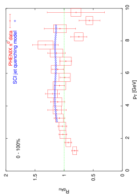
Figure 4: Model results for dAu (charged particles and neutral pions at $|\eta|<0.35$) and PHENIX $\pi^{0}$ data [40] (errorbars indicate statistical and boxes systematic errors)

The best results were obtained with $\alpha=0.25\,\mathrm{GeV^{2}}$ and are shown in Figure 4 together with the experimental data. The agreement is reasonably good for $3<p_{\perp}<9\,\mathrm{GeV}$, i.e.  where the $p_{\perp}$ is large enough for the model to be reliable and not too large so that the statistical error is moderate.

There is, however, a problem with the value of $\alpha=0.25\,\mathrm{GeV^{2}}$: One might want to interpret it as the square of the mean momentum transfer per scattering because of the way the model is constructed (Ch. 5 and 2). But the momentum transfer should not exceed 0.2 GeV if the proton is supposed to interact as a whole. This number is motivated by the uncertainty principle: The size of a proton is roughly 1 fm and a resolution of $1\,\mathrm{fm^{-1}}$ corresponds to a momentum transfer of 0.2 GeV. $\alpha$ being considerably larger than $0.04\,\mathrm{GeV^{2}}$ can be seen as evidence for other effects that build up additional transverse momentum. However, also a highly excited or dissociated proton interacts so that a larger value of $\alpha$ may be reasonable. The model for the Cronin effect used here is then an effective description that should not be taken too literally.

A variation of $\alpha$ by $\pm 0.1\,\mathrm{GeV^{2}}$ leads to only small changes with the result still being consistent with the data.

Figure 5 shows that the broadening of the intrinsic $k_{\perp}$ also has a small influence on the 2-particle azimuthal correlation. The fraction of events containing trigger particles is slightly increased from $3.16\cdot 10^{-3}$ in pp to $3.75\cdot 10^{-3}$.

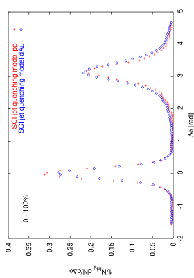
Figure 5: 2-particle azimuthal correlation in the SCI jet quenching model for pp and dAu collisions

2 Nuclear Modification Factor

The model results for the nuclear modification factor are shown in Figure 6 together with the experimental data for five different centrality classes. In the most central and most peripheral class the effect of the $k_{\perp}$-broadening without scatterings is shown in addition. It naturally increases with centrality because the nuclear overlap is much larger in central collisions. Thus the Cronin effect counteracts the partonic energy loss which is larger than it seems at first sight.

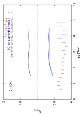
Figure 6: Model results for the nuclear modification factor with constant energy density for different centrality classes and PHENIX data [51], for 0-10% and 80-92% centrality also the effect of only $k_{\perp}$-broadening without partonic energy loss is shown

The approximately flat shape of $R_{\mathrm{AuAu}}$ for $p_{\perp}>3\,\mathrm{GeV}$ is well reproduced by the model. There is a slight increase in the range between 3 and 4-5 GeV that is caused by the $p_{\perp}$-cut on the matrix element. Because the intrinsic $k_{\perp}$ has to be added to the momentum transfer in the hard scattering, there are too few particles produced also above the threshold. The effect is more pronounced in nucleus-nucleus collisions due to the Cronin effect and thereore it doesn’t cancel completely in the ratio. As expected it increases with centrality and also reaches out to higher $p_{\perp}$ in more central events.

In the most peripheral class the model result is in agreement with the data but is somewhat low. The situation is slightly better in 60-70% but already in 40-50% the model result falls behind the data which decrease faster. The trend advances in the two central classes so that in the 0-10% bin the model gives roughly 50% of the effect observed in the data. The centrality dependence of the model result is rather weak so that it is practically impossible to identify the functional dependence.

With the non-uniform energy density distribution the result for 0-10% centrality is nearly identical with the one obtained with a constant energy density. But the increase when going to more peripheral collisions is stronger because the mean energy density decreases. It thus agrees better with the data than the other approach. This is also in reflected in Figure 8 where it becomes clear that the model follows the data for peripheral events, but then it levels off and stays approximately constant. In fact, the model depends quadratically on the centrality, there is no linear contribution. As will be discussed in Chapter 10 this is related to the dependence of the energy loss per interaction on the parton energy. Figure 9 shows the energy loss in the interaction with the first plasma gluon (interaction probability is 1 in this case) for light quarks as a function of the initial quark energy. Even for the highest energies the energy loss rises slightly (the averaged values after 10 scatterings are below those after only one interaction). On the other hand, quarks with very small energy gain energy because the thermal energy of the environment is higher than the quark energy.

Figure 8: Comparison of the centrality dependence of the model with inhomogeneous energy density profile to PHENIX data [51]

Figure 9: Dependence of the energy loss per scattering on the initial energy of the quark for $u$ and $d$ quarks, scattering centre is the first gluon (”10 scatterings” denotes 10 interactions with the same gluon)

3 Azimuthal Correlation

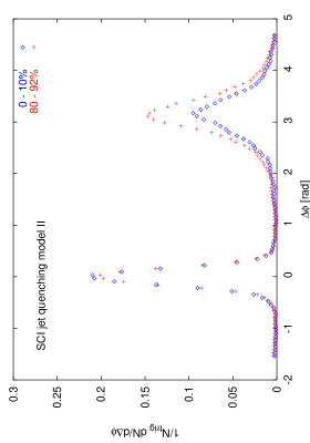
Figure 10: 2-particle azimuthal correlation from the model with constant (upper figure) and non-uniform energy density profile (lower figure) in peripheral (80-92%) and central collisions (0-10%)

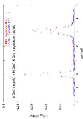
Figure 11: 2-particle azimuthal correlation for the Toymodel II b $\alpha$ with $\Delta E\propto N_{g}^{2}E$ and Toymodel II b $\gamma$ with $\Delta E\propto N_{g}^{2}$ for 0-10% centrality, trigger particles satisfy $8\,\mathrm{GeV}<p_{\perp}(\mathrm{trig})<10\,\mathrm{GeV}$ and associated particles have $6\,\mathrm{GeV}<p_{\perp}(\mathrm{assoc})<p_{\perp}(\mathrm{trig})$

The 2-particle azimuthal correlations for the two versions of the model are shown in Figure 10. There is a suppression of the away-side jet but no disappearance as in the data. Again the ansatz with an inhomogeneous energy density profile leads to a bigger effect. But while the Cronin effect counteracted the energy loss in the case of the nuclear modification factor, it now contributes to the jet quenching (Fig. 11). It leads to an away-side peak that is lower in central than in peripheral events, although it does not help on average (Fig. 5).

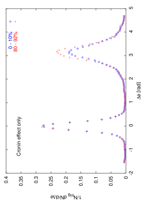
Figure 11: Azimuthal correlation in AuAu collisions with only Cronin effect (no scattering) for central and peripheral events

The near-side jet remains unchanged, but as discussed already in Section 2 this does not necessarily mean that the respective parton has not suffered energy loss. Since the partons are assumed to hadronise outside the QGP and ordinary vacuum fragmentation functions are used, the shape and the integral of the near-side peak are determined only by the momentum of the partons. The energy loss in the QGP shifts the parton $p_{\perp}$-spectrum to smaller momenta so that the overall yield of partons, that have enough energy to produce a trigger particle, is smaller. But since the 2-particle azimuthal correlation is normalized to the number of trigger particles and contains no information about the rate at which these particles are produced, this effect is invisible. However, there is a certain sensitivity to the shape of the parton $p_{\perp}$-spectrum because a more energetic parton will on average produce more associated particles. A flat spectrum will thus lead to a near-side peak with a larger area than a steeply falling spectrum because the relative contribution from partons with very high momenta is smaller in the latter case.

It is thus oversimplified to conclude that the partons producing trigger particles have not lost a substantial amount of energy and therefore stem form the periphery of the QGP. In fact, it can easily be shown that this is not the case. Figure 12 shows the results from a simulation with the SCI jet quenching model II where all hard scattering points were placed in a 0.5 fm thick shell at the edge of the overlap region ($b=0$). At first sight it is surprising that the jet quenching is very weak in this configuration but it can be explained as a mainly geometrical effect: If a parton is emitted from the surface with random direction in the transverse plane (this is the case for hard scattering) only a range of $\sim\pi/2$ in angle will lead to a sizable path through the plasma. Furthermore, the constituent density is much smaller near the edge than in the centre. But while a parton directed towards the centre of the QGP moves inward, the number density drops rapidly so that the parton never reaches a region of high density. The lifetime of the QGP is, with the parameters chosen here, $\tau_{f}\simeq 5\,\mathrm{fm/c}$ so that it hadronises even before the parton has reached the centre. The sum of these effects leads to the very weak jet quenching observed in Figure 12. The jet quenching increases with the thickness of the shell until for a thickness that equals the nuclear radius the original result for central collisions is recovered. The result is very similar for a constant energy density profile. This means that the observed hadrons are the fragmentation products of partons that come from practically everywhere in the overlap region.

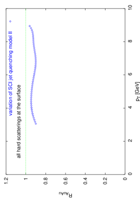
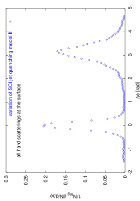
Figure 12: Results of the simulation with the SCI jet quenching model II but now all hard scattering points lie in a narrow shell at the edge, centrality is 0%

To get a substantial suppression of the away-side jet one parton has to lose much more energy than the other one. Since the crucial quantity for energy loss is the number density of constituent gluons, a situation where one parton encounters much more gluos is needed. There are several reasons why this is hard to achieve (and thus the effect on the azimuthal correlation is so small). Firstly the hard scattering points are concentrated towards the centre of the QGP and consequently the difference between the path lengths in the plasma of the two scattered partons is typically small. What makes the situation even worse is that the gluon density falls like $\tau^{-1}$. In fact, the energy loss per scattering increases as the temperature falls but the decrease in number density prevails (the consituent gluon energy is proportional to $\tau^{-1/3}$ only). This means that most of the energy loss happens at early times and small differences in path length are further reduced because the plasma is already quite dilute when the first parton leaves the overlap region. It is also seen in Figure 13, which shows the specific energy loss of light quarks as a function of the path length in the QGP. Quarks with low momentum gain energy because they are below the thermal energy in the beginning. They are also more sensitive to the plasma gluon energy than more energetic quarks, i.e. they follow the evolution of the QGP more closely.

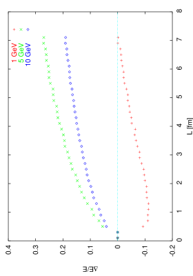
Figure 13: Specific energy loss of monoergetic light quarks emitted from the centre of the QGP with $\theta=\pi/4$, energy density is homogeneous

Furthermore, the QGP lifetime limits the possible path length differences in central collisions. Even for parton pairs that happen to be produced at the surface the path length difference cannot exceed the lifetime of $\sim 5\,\mathrm{fm}$. The model with the non-uniform energy density profile works better because it helps to amplify differences. If the hard scattering occured not directly in the centre the parton with the longer path traverses the denser central region and experiences more interactions than the other one which only moves through the more dilute outer parts of the QGP.

The asymmetry between the two hard scattered partons is enhanced by the matrix element since $\sim$50% of all parton level processes are $q+g\to q+g$ scatterings. The gluons interact more strongly and lose more energy than the quarks.

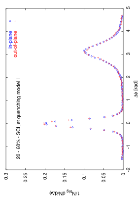
Figure 14: Correlation of the 2-particle azimuthal correlation with the reaction plane from the model with constant (upper figure) and non-uniform energy density profile lower figure) in mid-central collisions (20-60%)

In Figure 14 the correlation with the reaction plane is shown for mid-central events. In both cases there is no difference between the particles emitted in-plane and out-of-plane. The reason is that this observable suffers even more from the problems with the similar path lengths. The mean radius of the overlap region is 3.0 fm in-plane and 4.3 fm out-of-plane for 40% centrality. The difference is at most 1.3 fm in the whole range from 20 to 60% centrality so that the differences in path length of the two partons are small. Due to the other difficulties discussed before, it is not surprising that there is no visible effect on the azimuthal correlation.

3 Discussion

The SCI jet quenching model yields good results for the nuclear modification factor. The shape is similar to the data, namely approximately flat for $p_{\perp}>3\,\mathrm{GeV}$ and the magnitude can reach 50% of the observed effect in central collisions. The rest is presumably due to gluon bremsstrahlung which should naturally come along with the scatterings. The centrality dependence is, however, not linear as in the data but quadratic. It is not clear how this will change when gluon bremsstrahlung is included.

There is also a clear suppression of the away-side jet but the effect is much smaller than observed in data. The reasons for this are mostly understood: The hard scattering points are concentrated towards the centre of the QGP, the gluon density in the plasma falls rapidly and the lifetime limits the available path length differences between hard scattered partons. These are not details of this model but very general features.

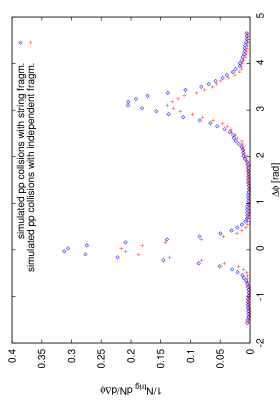
Figure 15: 2-particle azimuthal correlations in pp collisions for different fragmentation schemes

Another aspect is that the azimuthal correlation depends on the details of the fragmentation scheme. This is illustrated in Figure 15 which shows a comparison of Lund string fragmentation to independent fragmentation in pp simulations. The fragmentation function is the same in both cases (namely the Lund symmetric function). The independent fragmentation scheme produces somewhat less particles at midrapidity than the string fragmentation, but this is a small effect (the ratio of the $p_{\perp}$- spectra is $\sim 0.95$). For the 2-particle azimuthal correlation, however, this makes a big difference. Modifications of the fragmentation scheme and function are a point that has not been addressed in detail in this model but it is propbable that the presence of a QGP will also influence the fragmentation. This may lead to substantial changes in the azimuthal correlations, a softer fragmentation function for instance will enhance the suppression of the away-side jet.

Still it can be concluded that it is indeed possible to obtain a considerable contribution to the observed jet quenching from energy loss due to soft scatterings. The scenario with an energy density that is higher near the centre that at the edge of the QGP yields better results.

The energy loss per scattering is governed by the width of the $t$ distribution $\sigma_{t}$ and, to a smaller extent, the gluon mass $m_{g}$. A more massive gluon leads to a smaller energy loss. These parameters affect the overall energy loss and the centrality dependence.

The QGP formation time, initial energy density and critical temperature determine the number of scatterings but don’t affect the centrality dependence. A shorter formation time for example will add a certain number of encountered gluons to each parton irrespective of the centrality. Because of the high energy density in the early stage the overall energy loss depends quite strongly on the formation time and moderately on the initial energy density but hardly on the critical temperature.

The Cronin parameter is fixed independently with the help of the dAu data but there is still some freedom. A stronger $k_{\perp}$-broadening reduces the energy loss such that the centrality dependence of $R_{\mathrm{AuAu}}$ becomes flatter but it increases the suppression of the away-side jet in central collisions.

The effects of a hadronic layer around the plasma phase have not been studied here, but their overall characteristics can be qualitatively described. It would decrease the energy loss, but not very much as long as the hadronic layer is thin. This may in turn alter the influence of the centrality, depending on how the thickness changes with it. A more important effect could enter in connection with modified fragmentation. Partons that originate from scatterings in the hadronic layer may (depending on their direction of motion) escape without any interactions and hadronise as in vacuum. This has a potentially sizable impact on the azimuthal correlation.

Chapter 10 Exploring General Properties of Partonic Energy Loss

1 Motivation

It has been shown in Section 6 that the dependence of the energy loss $\Delta E$ on the parton energy $E$ and the path length $L$ (in a static medium) is sensitive to the physics of the energy loss mechanism. Matter induced gluon radiation can for instance lead to a typical $L^{2}$-dependence, if there are coherence effects. The energy loss by incoherent scatterings on the other hand is proportional to $L$. It is thus obvious to ask if it is possible, with the presently available data on jet quenching, to distinguish between different scenarios.

Now it is fortunate that the SCI jet quenching model is constructed in a modular fashion. It is thus possible to keep the model for the QGP but replace the energy loss by something less specific, so that different dependencies can be tested and compared to data. This can of course not replace a physical model, but it can easily be used to investigate if the data favour a certain type of energy loss mechanism.

2 Energy Loss in the Toymodel

The only part of the model that is different from the SCI jet quenching model is the energy loss. It is not simulated explicitely in the framework of the Toymodel, instead a certain amount of energy is substracted for each parton and deflection is not taken into account. This very general ansatz makes it possible to explore different dependencies of the overall energy loss. Since the path length is not a meaningful quantity in an expanding QGP, the number of plasma gluons $N_{g}$, that a parton encounters on its way, is used as a measure for the ”amount” of plasma seen by a parton (this is sensible since also for gluon bremsstrahlung the number of scatterings is the important quantity). The dependence of the energy loss on $N_{g}$ and on the parton energy can hence be varied according to the different cases listed in Table 1. The constant of proportionality is a free parameter that has to be adjusted. Again gluons lose more energy than quarks, in the Toymodel this is achieved by doubling the parameter. If the energy of a parton drops below a certain value $\mu_{\mathrm{th}}+\sigma_{\mathrm{th}}$, it is assigned a new momentum vector with energy picked from a Gaussian with mean $\mu_{\mathrm{th}}$ and width $\sigma_{\mathrm{th}}$, the direction of motion is chosen randomly. This is of course a very rough way to model the thermalisation of partons, but since they are anyway far below the trustworthy region in $p_{\perp}$ of the model the details of the process are not important.

Table 1: Versions of energy loss in the Toymodel, energies are in units of 1 GeV

Name	Dependencies			Constant
	path length	energy	energy density
Toymodel I a $\alpha$	$N_{g}$	$E$	uniform	$0.065\,\mathrm{GeV}$
Toymodel I b $\alpha$	$N_{g}^{2}$	$E$	uniform	$0.016\,\mathrm{GeV}$
Toymodel II a $\alpha$	$N_{g}$	$E$	non-uniform	$0.070\,\mathrm{GeV}$
Toymodel II b $\alpha$	$N_{g}^{2}$	$E$	non-uniform	$0.018\,\mathrm{GeV}$
Toymodel II a $\beta$	$N_{g}$	$\sqrt{E}$	non-uniform	$0.300\,\mathrm{GeV}$
Toymodel II b $\beta$	$N_{g}^{2}$	$\sqrt{E}$	non-uniform	$0.020\,\mathrm{GeV}$
Toymodel II a $\gamma$	$N_{g}$	const.	non-uniform	$0.425\,\mathrm{GeV}$
Toymodel II b $\gamma$	$N_{g}^{2}$	const.	non-uniform	$0.200\,\mathrm{GeV}$

The other parameters that describe the QGP are the same as in the SCI jet quenching model. A complete list with the default values is given in Table 2. The fragmentation scheme is again independent fragmentation.

Table 2: Parameters of the Toymodel, their default values and constraints

	Parameter		default value	sensible range
QGP	size of hadronic layer (only with homogeneous energy density)	$d$	0 fm	0…3 fm (?)
	QGP formation time	$\tau_{i}$	0.6 fm/c	0.2…1 fm/c [68]
	initial energy density ($\tau_{0}=1\,\mathrm{fm/c}$)	$\epsilon_{0}$	$5.5\,\mathrm{GeV\,fm^{-3}}$	4…6.5 GeV fm-3 [68]
	critical temperature	$T_{c}$	0.17 GeV	0.17…0.18 GeV
	radius of parton cylinder	$R_{\mathrm{cyl}}$	0.3 fm	$\sim$ 0.3 fm
Cronin effect	increase of $\sigma_{k_{\perp}}^{2}$ per scattering	$\alpha$	$0.25\,\mathrm{GeV^{2}}$	?
energy	mean thermal energy	$\mu_{\mathrm{th}}$	0.6 GeV
loss	width of th. energy distr.	$\sigma_{\mathrm{th}}$	0.1 GeV
	constant of proportionality

The constant is adjusted in one centrality bin (either the most central or the most peripheral) and then the other classes are generated with the same value.

3 Results

In this section only a fraction of the results is shown, the complete set can be found in Appendix 13. The shape of the nuclear modification factor is very similar in all versions: It is nearly flat with a tendency to decrease slightly towards high $p_{\perp}$, only when $\Delta E$ is independent of $E$ it rises. The centrality dependence and the azimuthal correlation are more interesting, because they are sensitive to the differences in the model assumed for the energy loss.

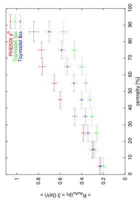
Figure 1: Centrality dependence of $R_{\mathrm{AuAu}}$ for the Toymodel I a $\alpha$ with $\Delta E\propto N_{g}E$ and Toymodel I b $\alpha$ with $\Delta E\propto N_{g}^{2}E$, both with uniform energy density profile

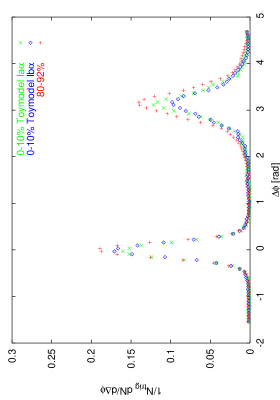
Figure 2: 2-particle azimuthal correlation for the Toymodel I a $\alpha$ with $\Delta E\propto N_{g}E$ and Toymodel I b $\alpha$ with $\Delta E\propto N_{g}^{2}E$, both with uniform energy density profile, the 80-92% data are the same in both cases

Figure 1 shows the centrality dependence of $R_{\mathrm{AuAu}}$ for the configurations with a homogeneous energy density profile Toymodel I a $\alpha$ and I b $\alpha$. The shape is in both cases similar, although the linear version (I a $\alpha$) seems to be somewhat flatter. The course of I a $\alpha$ is mildly curved while I b $\alpha$ is more straight. Both model results are significantly flatter than the data. The absolut magnitude of the nuclear modification factor is not meaningful, since it is governed by a free parameter.

The effect on the 2-particle correlation is in both cases small, but stronger in I b $\alpha$ (Fig. 2). So altogether the configuration with $\Delta E\propto N_{g}^{2}$ appears to be slightly closer to the experimental data.

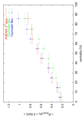
Figure 3: Centrality dependence of $R_{\mathrm{AuAu}}$ for the Toymodel II a $\alpha$ with $\Delta E\propto N_{g}E$ and Toymodel II b $\alpha$ with $\Delta E\propto N_{g}^{2}E$, both with non-uniform energy density profile

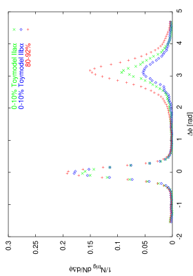
Figure 4: 2-particle azimuthal correlation for the Toymodel II a $\alpha$ with $\Delta E\propto N_{g}E$ and Toymodel II b $\alpha$ with $\Delta E\propto N_{g}^{2}E$, both with non-uniform energy density profile, the 80-92% data are the same in both cases

In the configuration with a non-uniform energy density the mean energy density increases with centrality. Thus the expectation is that the shape of the centrality dependence of $R_{\mathrm{AuAu}}$ is steeper than with a constant energy density. This is in fact observed (Fig. 3). Although both calculation results are slightly curved, they now give a reasonably good description of the data. The bending is again more distinct in the linear ansatz.

The suppression of the away-side jet has also improved in both cases as compared to Toymodel I (Fig. 4). This matches with the observation made with the SCI jet-quenching model where also the inhomogeneous energy density distribution yields better results.

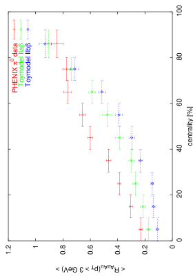
Figure 5: Centrality dependence of $R_{\mathrm{AuAu}}$ for the Toymodel II a $\beta$ with $\Delta E\propto N_{g}\sqrt{E}$ and Toymodel II b $\beta$ with $\Delta E\propto N_{g}^{2}\sqrt{E}$, both with non-uniform energy density profile

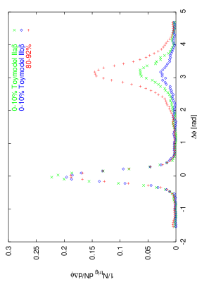
Figure 6: 2-particle azimuthal correlation for the Toymodel II a $\beta$ with $\Delta E\propto N_{g}\sqrt{E}$ and Toymodel II b $\beta$ with $\Delta E\propto N_{g}^{2}\sqrt{E}$, both with non-uniform energy density profile, the 80-92% data are the same in both cases

When $\Delta E\propto\sqrt{E}$ the centrality dependence is parabolic (Fig. 5) without a linear component and hence qualitatively different from the data. The two scenarios Toymodel II a $\beta$ and II b $\beta$ are again very similar, but this time the curvature is somewhat stronger in the quadratic setup II b $\beta$.

In the 2-particle correlation on the other hand the situation is as before: The suppression obtained with II b $\beta$ is clearly stronger than with II a $\beta$. The effect is even bigger than before and has reached a reduction by more than 50% (Fig. 6).

Surprisingly the results of the ansatz with $\Delta E$ independent of $E$ are very similar to those obtained with $\Delta E\propto E$. The centrality dependence is now linear in both cases and again the II a $\gamma$ is slightly flatter than II b $\gamma$. While the centrality dependence of $R_{\mathrm{AuAu}}$ agrees quite well with the data the azimuthal correlation is not as convincing. There is a suppression which is again stronger for the quadratic version II b $\gamma$, but this is still far from a disappearance. It is also slightly worse than the results obtained with $\Delta E\propto E$.

4 Summary and Discussion

In summary, the differences in $R_{\mathrm{AuAu}}$ and its centrality dependence between the configurations with $\Delta E\propto N_{g}$ and $\Delta E\propto N_{g}^{2}$ are small. $\Delta E\propto N_{g}^{2}$ has the tendency to look slightly better and also the suppression of the away-side jet is stronger. However, these differences are not big enough to come to a clear cut conclusion. The $N_{g}^{2}$ dependence seems to be favoured, but the $N_{g}$ dependence is not ruled out.

The situation becomes partly clearer when it comes to the energy dependence. Here the $\Delta E\propto\sqrt{E}$ scenario leads to a centrality dependence of $R_{\mathrm{AuAu}}$ that has a clear parabolic shape and is thus qualitatively different from the linear behaviour observed in the data. The suppression of the away-side jet is stronger than in the other versions, but since this observable is not very sensitive to the energy dependence this is not a strong argument. Besides, the azimuthal correlation is obviously quite sensitive to details of the fragmentation which is not well under control in this model. So it is justified to conclude that $\Delta E\propto\sqrt{E}$ is clearly disfavoured.

But then it becomes more difficult since it is practically impossible to distinguish between $\Delta E\propto E$ and $\Delta E$ independent of $E$. Perhaps the centrality dependence is slightly better in the latter case, but for the azimuthal correlation it is just the other way around. There are minimal differences in the shape of $R_{\mathrm{AuAu}}$: It has a tendency to fall mildly when $\Delta E\propto E$ and rise when $\Delta E$ does not depend on $E$, but the data don’t favour one or the other alternative (Fig. 9). With the presently available data it is therefore not possible to differentiate between the two options and also with better statistics it is not trivial since the differences in $R_{\mathrm{AuAu}}$ are also at higher $p_{\perp}$ not big.

There is a difference between the two scenarios when going to higher $p_{\perp}$ with the 2-particle azimuthal correlation. This is shown with an example for the $\Delta E\propto N_{g}^{2}$ configurations in Figure 10 and 11. The suppression of the away-side jet is clearly stronger in Toymodel II b $\alpha$ than in II b $\gamma$. It is also observed that the height of the away-side peak relative to the near-side peak increases when going to higher $p_{\perp}$, although the nuclear modification factor stays more or less flat. The increase is thus not due to a ”punch-through”, i.e. particles that have so much energy that they lose only a very small fraction and emerge nearly undisturbed from the plasma. In fact, it is connected to the observation that the jet quenching becomes inefficient when the hard scattering occurs near the surface of the QGP made in Section 3. When the trigger condition gets more restrictive only jets from partons that suffered hardly any energy loss are selected. This means that the hard scattering points of the selected events move more and more towards the surface and the quenching becomes more inefficient. Consequently the away-side jet reappears even though the nuclear modification factor stays constant.

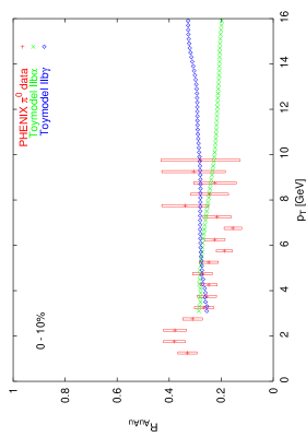
Figure 9: $R_{\mathrm{AuAu}}$ in Toymodel II b $\alpha$ with $\Delta E\propto N_{g}^{2}E$ and Toymodel II b $\gamma$ with $\Delta E\propto N_{g}^{2}$

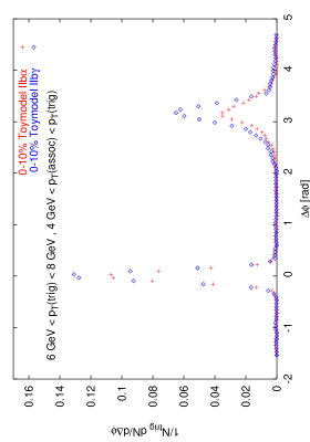
Figure 10: 2-particle azimuthal correlation for the Toymodel II b $\alpha$ with $\Delta E\propto N_{g}^{2}E$ and Toymodel II b $\gamma$ with $\Delta E\propto N_{g}^{2}$ for 0-10% centrality, trigger particles satisfy $6\,\mathrm{GeV}<p_{\perp}(\mathrm{trig})<8\,\mathrm{GeV}$ and associated particles have $4\,\mathrm{GeV}<p_{\perp}(\mathrm{assoc})<p_{\perp}(\mathrm{trig})$

The results of this section show that the gluon bremsstrahlung scenario in the high energy limit (Eq. 58) is within the bounds of possibility while the result obtained for $L>L_{\mathrm{cr}}$ (Eq. 59) seems to be ruled out, at least when it is not combined with some other mechanism.

The SCI jet quenching model also has an energy dependence (Fig. 9) which is not consistent with the data. But here it is clear that there is an additional effect missing since it can account only for 50% of the observed jet quenching. And it cannot be expected that the SCI jet quenching model describes the whole effect. So there is still freedom to resolve the present difficulties when the model is combined with induced gluon radiation (or possibly even more effects) to get a full description of the energy loss.

The inhomogeneous energy density distribution works better than the homogeneous. This agrees with the findings of the SCI jet quenching model and there is no reason why the energy density should be homogeneous. Concerning a possible hadronic layer the same considerations as for the SCI jet quenching model apply, namely that it can have an impact on the influence of the centrality depending on how the thickness of the layer changes with centrality.

The fact that the centrality dependence does not level off and become flat at a certain level illustrates that the available path lengths are limited predominantly by the geometry and not by the QGP lifetime. Otherwise, at some point an increase of the size of the overlap region (i.e. going to more central events) would not result in longer path lengths and the nuclear modification factor would be unchanged.

Since the Toymodel makes use of the same model for the geometry (e.g. distribution of hard scatterings in the overlap region), the QGP etc. as the SCI jet quenching model, it is expected to suffer from the same problems with the 2-particle azimuthal correlations. However, because they are mainly due to very general properties of the QGP one would think that the energy loss mechanism has to compensate the difficulties. The fact that even those versions of the Toymodel, which yield a good description of the nuclear modification factor, fail to describe the disappearance of the away-side jet strengthens the case for the hypothesis that the azimuthal correlation is fairly sensitive to the fragmentation scheme and function. However, it seems that it is also influenced by the path length dependence of the energy loss mechanism.

The nuclear modification factor on the other hand was found to depend only very weakly on the exact energy and path length correlation with the energy loss and is also insensitive to the energy density distribution. The centrality dependence of $R_{\mathrm{AuAu}}$ probes mainly the energy dependence.

Now one can also try to answer the question of how the linear centrality dependence comes about. Strangely enough, it seems that a lot of different effects conspire to yield a very simple form in the end. It has been shown that apart from the geometry (and the QGP lifetime) also the Cronin effect, the energy density distribution, the energy dependence of the energy loss and to some extend the impact of the path length on the energy loss influence the behaviour with the centrality.

Chapter 11 Conclusions and Outlook

Given the wealth of different observables that point towards QGP formation at RHIC, it seems that indeed the long-sought quark-gluon plasma has been created. Among them, the jet quenching plays an important role. For SPS the question whether a QGP is formed or not is not so easy to answer. But as has been shown in this thesis, the shapes of the $p_{\perp}$-spectra are not very different from those measured at RHIC. Since this applies also for other observables, it is very well conceivable that the phase boundary has already been crossed in central collisions at SPS. However, from SPS data it is very difficult to investigate the properties of the new state of matter. This is to some extend possible at RHIC, but still a very difficult task that requires a profound understanding in particular of the high-$p_{\perp}$ physics and the jet quenching.

It was shown that soft rescattering of a hard scattered parton in a QGP can contribute significantly to the overall energy loss. With the model introduced in the first part of this thesis, roughly 50% of the observed effect in central collisions was reproduced. The magnitude depends on the momentum transfer per scattering which is a parameter, but it is clear that losses induced by scattering may not simply be neglected.

It is not a problem that the model cannot account for the whole effect, since it cannot be considered complete in the sense that all processes contributing to the energy loss are included. The most obvious example is medium induced gluon radiation. It seems natural that scattering of the parton should induce gluon bremsstrahlung resulting in further energy loss. Additional processes will of course also change the centrality dependence so that at this stage it should not be overemphasised that the centrality dependence found in the SCI jet quenching model does not match the data.

Nevertheless, the model is in two respects not very well motivated. First, it could be argued that the assumption of independent scatterings is not justified, at least at the early times when the density in the QGP is high, since soft interactions happen on relatively long time scales. Then interferences might become important and it is not clear how they should be treated in a Monte Carlo generator. The second point is that since the momentum transfer is small it is impossible to resolve individual gluons. This would mean that the plasma has to be treated as a colour charged gluonic field with which the partons would nevertheless interact. But the parton-field interaction may not be very different from the parton-gluon interaction. Since there is poor theoretical guidance for soft interactions, the parton-gluon scattering can be used as a model.

It should also be noted that the (single) gluon exchange model should not be taken too literally. The Gaussian momentum transfer should rather be interpreted as due to a superposition of many-gluon exchanges. The exact details of this process are not relevant for this study.

The main conclusion is unaffected by these problems that are unescapable when dealing with soft physics: Soft scattering can result in a sizable energy loss.

The lesson to learn from the investigations of the overall features of partonic energy loss is that it is difficult to distinguish between different scenarios given the presently available data. $\Delta E\propto\sqrt{E}$ seems unprobable because it yields the wrong centrality dependence of $R_{\mathrm{AuAu}}$. But $\Delta E\propto E$ and $\Delta E\propto\mathrm{const}$ are practically undistinguishable, this will maybe become possible with better data at higher $p_{\perp}$. $\Delta E\propto N_{g}$ and $\Delta E\propto N_{g}^{2}$ are also similar, $\Delta E\propto N_{g}^{2}$ looks slightly better. This may be interpreted as a hint for coherent gluon radiation but it is not a strong indication. In summary, it has not been possible to get to a clear cut conclusion for or against coherent gluon bremsstrahlung.

The 2-particle azimuthal correlation seems to depend on details of the fragmentation procedure, an issue that has not been addressed in great detail in this study. This makes it very difficult to judge the results of the models but also to understand the data when attention is paid to the details. Beyond that, the azimuthal correlation shows a certain sensitivity to the path length dependence of the energy loss. In contrast the nuclear modification factor is insensitive to many details and the centrality dependence of $R_{\mathrm{AuAu}}$ is ruled mainly by the energy dependence.

For the future it is desirable to gain a better understanding of the interplay of scattering and gluon radiation. Unfortunately, including radiation in the SCI jet quenching model is not free of difficulties. While incoherent radiation is rather straightforward the coherence effects are extremely difficult to handle in a Monte Carlo framework.

Another unsolved problem are the medium modifications to hadronisation. This is also highly non-trivial, mainly due to lack of information. Moreover, it is difficult to disentangle the effect of modified fragmentation from other medium modifications. Hopefully, one can get some guidance from the observation of modified fragmentation in cold nuclear matter (e.g. [69]).

If one wants to fully exploit jet tomography, i.e. use the jet quenching to determine the properties of the QGP, one first has to come to a consistent picture and get the partonic energy loss theoretically better under control. This means that further effort has to be made in order to gain a better understanding of the underlying physical principles.

Chapter 12 Fit Parameters for Identified Particle Spectra

Chapter 13 Complete Results from the Toymodel

References

- [1] A. Edin, G. Ingelman and J. Rathsman, Phys. Lett. B366 (1996) 371 and R. Enberg, G. Ingelman and N. Tîmneanu, Phys. Rev. D64 (2001) 114015
- [2] O. Nachtmann, Elementary Particle Physics, Springer Verlag, Berlin (1990)
- [3] R. K. Ellis, W. J. Stirling and B. R. Webber, QCD and Collider Physics, Cambridge University Press, Cambridge (1996)
- [4] B. Andersson, G. Gustafson, G. Ingelman and T. Sjöstrand, Phys. Rept. 97 (1983) 31
-
[5]
A. Krzywicki and B. Petersson, Phys. Rev. D6 (1972) 924
J. Finkelstein and R.D. Peccei, Phys. Rev. D6 (1972) 2606
R. D. Field and R. P. Feynman, Nucl. Phys. B149 (1979) 413 - [6] T. Sjöstrand, P. Eden, C. Friberg, L. Lönnblad, G. Miu, S. Mrenna and E. Norrbin, Computer Physics Commun. 135 (2001) 238
- [7] S. A. Bass, M. Gyulassy, H. Stöcker and W. Greiner, J. Phys. G25 (1999) R1
- [8] J. W. Harris and B. Müller, Ann. Rev. Nucl. Part. Sci. 46 (1996) 71
- [9] R. Snellings, nucl-ex/0310019
- [10] P. Braun-Munzinger, K. Redlich and J. Stachel, Quark Gluon Plasma 3, eds. R.C. Hwa and X.N. Wang, World Scientific Publishing
- [11] K. Geiger and B. Müller, Nucl. Phys. B369 (1992) 600
- [12] B. Anderson, G. Gustafson and B. Nilsson-Almqvist, Nucl. Phys. B281 (1987) 289
- [13] J. D. Bjorken, Phys. Rev. D27 (1983) 140
- [14] R. B. Clare and D. Strottman, Phys. Reports 141 (1986) 179
- [15] E. Scomparin, Nucl. Phys. A681 (2001) 124c and references therein
- [16] S. Datta, F. Karsch, P. Petreczky and I. Wetzorke, J. Phys. G30 (2004) S1347
- [17] D. Zschiesche, L. Gerland, S. Schramm, J. Schaffner-Bielich, H. Stöcker and W. Greiner, Nucl. Phys. A681 (2001) 34c
- [18] S. Scherer et al., Progess in Particle and Nuclear Physics, 42 (1999) 279
- [19] A. Andronic, P. Braun-Munzinger, K. Redlich and J. Stachel, Phys. Lett. B571 (2003) 36
- [20] V. D. Barger and R. J. N. Phillips, Collider Physics, Addison Wesley Publishing Company, (1997)
- [21] M. Jacob and P. V. Landshoff, Phys. Rep. 48 (1978) 285
- [22] R. Albrecht et al., WA80 Collaboration, Eur. Phys. J. C5 (1998) 255
- [23] X. N. Wang, Phys. Rev. C61 (2000) 064910
- [24] P. Levai, G. Papp, G. G. Barnafoldi and G. I. Fai, nucl-th/0306019
- [25] H. Baier,Y. L. Dokshitzer, A. H. Mueller, S. Peigné and D. Schiff, Nucl. Phys. B483 (1997) 291
-
[26]
K. J. Eskola, K. Kajantie and J. Lindfors, Nucl. Phys. B323 (1989)
37
see also http://www-aix.gsi.de/~misko/overlap - [27] L. D. Landau and E. M. Lifshitz, Course of Theoretical Physics Vol. V: Statistical Physics Pt. 1, Pergamon Press, Oxford (2001)
- [28] P. Braun-Munzinger and J. Stachel, Nucl. Phys. A638 (1998) 3
- [29] J. Stachel, Nucl. Phys. A654 (1999) 119c
- [30] J. W. Cronin et al. , Phys. Rev. D11 (1975) 3105
- [31] A. Accardi, hep-ph/0212148, Contribution to CERN Yellow Report on Hard Probes in Heavy Ion Collisions at the LHC
- [32] X. N. Wang, Phys. Rev. C61 (2000) 064910
- [33] Y. Zhang, G. Fai, G. Papp, G. G. Barnafoldi and P. Levai, Phys. Rev. C65 (2002) 034903
- [34] B. Alessandro et al., NA50 Collaboration, Eur. Phys. J. C39 (2005) 335
- [35] S. S. Adler et al., PHENIX collaboration, Phys. Rev. C69 (2004) 034910
- [36] J. Adams et al., STAR collaboration, Phys. Rev. Lett. 91 (2003) 172302
- [37] I. Arsene et al., BRAHMS collaboration, Phys. Rev. Lett. 91 (2003) 072305
- [38] B. B. Back et al., PHOBOS collaboration, Phys. Lett. B578 (2004) 297
- [39] D. Kharzeev, E. Levin and L. McLerran, Phys. Lett. B561 (2003) 93 and references therein and B. Müller, Phys. Rev. C67 (2003) 061901
- [40] S. S. Adler et al., PHENIX collaboration, Phys. Rev. Lett. 91 (2003) 072303
- [41] J. Adams et al., STAR collaboration, Phys. Rev. Lett. 91 (2003) 072304
- [42] S. S. Adler et al., PHENIX collaboration, Phys. Rev. Lett. 91 (2003) 172301
- [43] B. B. Back et al., PHOBOS collaboration, Phys. Rev. Lett. 91 (2003) 072302
- [44] C. Adler et al., STAR collaboration, Phys. Rev. Lett. 90 (2003) 082302
- [45] J. Adams et al., STAR collaboration, Phys. Rev. Lett. 93 (2004) 252301
- [46] J. Adams et al., STAR collaboration, Phys. Rev. Lett. 92 (2004) 182301
- [47] P. Braun-Munzinger, D. Magestro, K. Redlich, J. Stachel, Phys. Lett. B518 (2001) 41
- [48] P. Braun-Munzinger, J. Stachel, C. Wetterich, Phys. Lett. B596 (2004) 61
- [49] S. S. Adler et al., PHENIX collaboration, Phys. Rev. C69 (2004) 014901
- [50] P. Braun-Munzinger, I. Heppe, J. Stachel, Phys. Lett. B465 (1999) 15
- [51] S. S. Adler et al., PHENIX collaboration,Phys. Rev. Lett. 91 (2003) 072301
- [52] K. Adcox et al., PHENIX Collaboration, Phys. Rev. Lett. 88 (2002) 192302
- [53] S. S. Adler et al., PHENIX Collaboration, Phys. Rev. C96 (2004) 034909
- [54] J. Adams et al., STAR Collaboration, Phys. Rev. Lett. 92 (2004) 112301
- [55] F. Antinori et al., NA57 Collaboration, J. Phys. G30 (2004) 823
- [56] I. G. Bearden et al., NA44 Collaboration, Phys. Rev. C66 (2002) 044907
- [57] S. V. Afanasiev et al., NA49 Collaboration, Phys. Rev. C66 (2002) 054902
- [58] K. Adcox et al., PHENIX Collaboration, Phys. Rev. Lett. 89 (2002) 092302
- [59] C. Adler et al., STAR Collaboration, Phys. Rev. Lett. 89 (2002) 092301
- [60] T. Anticic et al., NA49 Collaboration, Phys. Rev. Lett. 93 (2004) 022302
- [61] M. van Leeuwen for the NA49 Collaboration, Nucl. Phys. A715 (2003) 161c
- [62] J. Slívová Doctoral Thesis, Heidelberg
- [63] M. M. Aggarwal et al., STAR Collaboration, Phys. Rev. Lett. 81 (1998) 4087
- [64] F. James, Rep. Prog. Phys. 43 (1980) 1145
- [65] J. Rathsman, Phys. Lett. B452 (1999) 364
- [66] S. J. Brodsky, R. Enberg, P. Hoyer and G. Ingelman, Phys. Rev. 71 (2005) 074020
- [67] I. Vitev, M. Gyulassy, Phys. Rev. Lett. 89 (2002) 252301
- [68] P. Huovinen, Nucl. Phys. A715 (2003) 299
- [69] A. Airapetian, HERMES Collaboration, Phys. Lett. B577 (2003) 37